Linear Algebra Written ExaminationsStudy Guide

Eduardo Corona Other Authors as they Join In

November 2, 2008

Contents

1 Vector Spaces and Matrix Operations 2

2 Linear Operators 2

3 Diagonalizable Operators 33.1 The Rayleigh Quotient and the Min-Max Theorem . . . . . . . . 43.2 Gershgorin�s Discs Theorem . . . . . . . . . . . . . . . . . . . . . 4

4 Hilbert Space Theory: Interior Product, Orthogonal Projectionand Adjoint Operators 54.1 Orthogonal Projection . . . . . . . . . . . . . . . . . . . . . . . . 74.2 The Gram-Schmidt Process and QR Factorization . . . . . . . . 84.3 Riesz Representation Theorem and The Adjoint Operator . . . . 9

5 Normal and Self-Adjoint Operators: Spectral Theorems andRelated Results 115.1 Unitary Operators . . . . . . . . . . . . . . . . . . . . . . . . . . 145.2 Positive Operators and Square Roots . . . . . . . . . . . . . . . . 15

6 Singular Value Decomposition and the Moore-Penrose Gener-alized Inverse 166.1 Singular Value Decomposition . . . . . . . . . . . . . . . . . . . . 166.2 The Moore-Penrose Generalized Inverse . . . . . . . . . . . . . . 186.3 The Polar Decomposition . . . . . . . . . . . . . . . . . . . . . . 19

7 Matrix Norms and Low Rank Approximation 197.1 The Frobenius Norm . . . . . . . . . . . . . . . . . . . . . . . . 197.2 Operator Norms . . . . . . . . . . . . . . . . . . . . . . . . . . . 207.3 Low Rank Matrix Approximation: . . . . . . . . . . . . . . . . . 21

1

8 Generalized Eigenvalues, the Jordan Canonical Form and eA 228.1 The Generalized Eigenspace K� . . . . . . . . . . . . . . . . . . . 238.2 A method to compute the Jordan Form: The points diagram . . 248.3 Applications: Matrix Powers and Power Series . . . . . . . . . . . 24

9 Nilpotent Operators 24

10 Other Important Matrix Factorizations 24

11 Other Topics (which appear in past exams) 24

12 Yet more Topics I can think of 25

1 Vector Spaces and Matrix Operations

2 Linear Operators

De�nition 1 Let U ,V be vector spaces =F (Usually F = R or C). ThenL(U; V ) = fT : U ! V j T is linearg: In particular, L(U;U) = L(U) is thespace of linear operators of U , and L(U;F ) = U� is its algebraic dual.

De�nition 2 Important Subspaces: Given W � V (subspace), T�1(W ) �U: In particular, we are interested in T�1(f0g) = Ker(T ): Also, if S � U; thenT (S) � U: We are most interested in T (U) = Ran(T ):

Theorem 3 U; V ev=F , dim(U) = n; dim(V ) = m: Given B = fu1; :::; ungbasis of U and B0 = fv1; :::; vmg basis of V; to each T 2 L(U; V ) we can associatea matrix [T ]B

0

B such that:

Tui = a1iv1 + :::+ amivm 8i 2 f1; ::;mg[T ]B

0

B = (aij) in Mm�n(F )

TU �! V

B l l B0

Fn �! Fm

[T ]B0

B

Conversely, given a matrix A 2Mm�n(F ); there is a unique TA 2 L(U; V ) suchthat A = [T ]B

0

B :

Proposition 4 Given T 2 L(U); there exist basis B and B0 of U such that:

[T ]B0

B =

�I 00 0

�B is constructed as an extension for a basis for Ker(T ); and B0 as an extensionfor fT (u)gu2B :

2

Theorem 5 (Rank and Nullity) dim(U) = dim(Ker(T ))+dim(Ran(T )): �(T ) =dim(Ker(T )) is known as the nullity of T; and r(T ) = dim(Ran(T )) as the rankof T:

Change of Basis: U; V ev=F; B and � basis of U; B0,�0 basis of V; thereexists P invertible such that:

[T ]B0

B = P [T ]�0

� P�1

P is a matrix that performs a change of coordinates. This means that, if twomatrices are similar, they represent the same linear operator using a di¤erentbasis. This further justi�es that key properties of matrices are preserved undersimilarity.

3 Diagonalizable Operators

If U = V (T;is a linear operator), it is natural to impose that both basis B andB0 are also the same. In this case, it is no longer generally true that we can�nd a basis B such that the corresponding matrix is diagonal. However, if thereexists a basis B such that [T ]B

0

B = � diagonal matrix, we say T is diagonalizable.

De�nition 6 V ev=F; T 2 L(V ). � 2 F is an eigenvalue of T if 9 v 2 V anonzero vector such that Tv = �v: All nonzero vectors such that this holds areknown as eigenvectors of T:

We can immediately derive, from this de�nition, that the existence of theeigenpair (�; v) (eigenvalue � and corresponding eigenvector v) is equivalent tothe existence of a nonzero solution v to

(T � �I)v = 0

This in turn tells us that the eigenvalues of T are those such that the operatorT � �I is not invertible. After selecting a basis B for V; this also means: u

det([T ]BB � �I) = 0

Which is called the characteristic equation of T . We notice this equationdoes not depend on the choice of basis B; since it is invariant under similarity:

det(PAP�1 � �I) = det(P (A� �I)P�1) = det(A� �I)

This equation �nally is equivalent to �nding the complex roots of a polyno-mial in �:We know this to be a really hard problem for n � 5, and a numericallyill-posed problem at that.

3

De�nition 7 V ev=F; T 2 L(V ), � an eigenvector of T: Then E� = fv 2 V jTv = �vg is the eigenspace for �:

Theorem 8 V ev=F of �nite dimension; T 2 L(V ): The following are equiva-lent:i) T is diagonalizableii) V has a basis of eigenvectors of Tiii) There exist subspaces W1; :::;Wn such that dim(Wi) = 1; T (Wi) � Wi andV =

Lni=1Wi

iv) V =Lk

i=1E�k with f�1; :::; �kg eigenvalues of Tv)Pk

i=1 dim(E�i) = dim(V )

Proposition 9 V ev=C; T 2 L(V ) then T has at least one eigenvalue (this is acorollary of the Fundamental Theorem of Algebra, applied to the characteristicequation).

Theorem 10 (Schur�s factorization) V ev=C; T 2 L(V ): There always existsa basis B such that [T ]B is upper triangular.

3.1 The Rayleigh Quotient and the Min-Max Theorem

3.2 Gershgorin�s Discs Theorem

Although calculating eigenvalues of a big matrix is a very di¢ cult problem(computationally and analytically), it is very easy to come up with regions onthe complex plane where all the eigenvalues of a particular operator T mustlie. This technique was �rst devised by the russian mathematician SemyonAranovich Gershgorin (1901� 1933):

Theorem 11 (Gershgorin, 1931) Let A = (aij) 2Mn(C): For each i 2 f1; ::; ng;we de�ne the ith "radius of A" as ri(A) =

Pj 6=i jaij j and the ith Gershgorin

disc asDi(A) = fz 2 C j jz � aiij < ri(A)

Then, if we de�ne �(A) = f� j � is an eigenvalue of Ag; it follows that:

�(A) �n[i=1

Di(A)

That is, all eigenvalues of A must lie inside one or more Gershgorin discs.

4

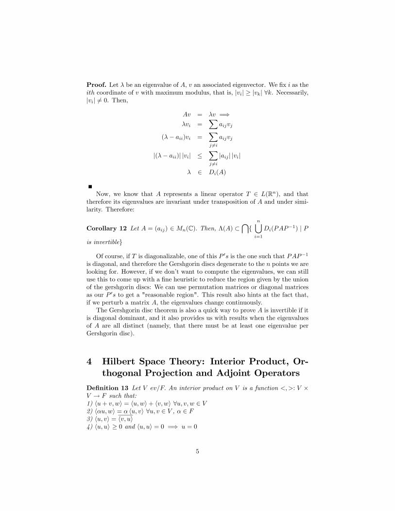
Proof. Let � be an eigenvalue of A; v an associated eigenvector. We �x i as theith coordinate of v with maximum modulus, that is, jvij � jvkj 8k. Necessarily,jvij 6= 0. Then,

Av = �v =)�vi =

Xaijvj

(�� aii)vi =Xj 6=i

aijvj

j(�� aii)j jvij �Xj 6=i

jaij j jvij

� 2 Di(A)

Now, we know that A represents a linear operator T 2 L(Rn), and thattherefore its eigenvalues are invariant under transposition of A and under simi-larity. Therefore:

Corollary 12 Let A = (aij) 2Mn(C): Then, �(A) �\f

n[i=1

Di(PAP�1) j P

is invertibleg

Of course, if T is diagonalizable, one of this P 0s is the one such that PAP�1

is diagonal, and therefore the Gershgorin discs degenerate to the n points we arelooking for. However, if we don�t want to compute the eigenvalues, we can stilluse this to come up with a �ne heuristic to reduce the region given by the unionof the gershgorin discs: We can use permutation matrices or diagonal matricesas our P 0s to get a "reasonable region". This result also hints at the fact that,if we perturb a matrix A, the eigenvalues change continuously.The Gershgorin disc theorem is also a quick way to prove A is invertible if it

is diagonal dominant, and it also provides us with results when the eigenvaluesof A are all distinct (namely, that there must be at least one eigenvalue perGershgorin disc).

4 Hilbert Space Theory: Interior Product, Or-thogonal Projection and Adjoint Operators

De�nition 13 Let V ev=F: An interior product on V is a function <;>: V �V ! F such that:1) hu+ v; wi = hu;wi+ hv; wi 8u; v; w 2 V2) h�u;wi = � hu; vi 8u; v 2 V , � 2 F3) hu; vi = hv; ui4) hu; ui � 0 and hu; ui = 0 =) u = 0

5

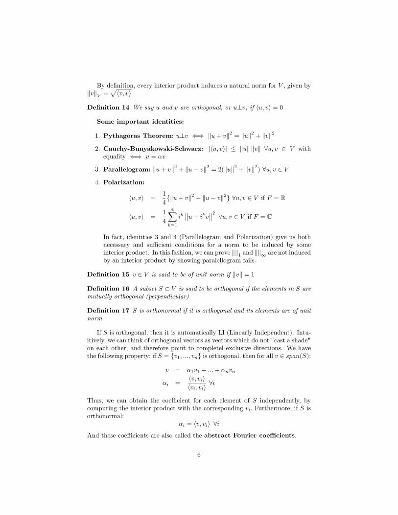
By de�nition, every interior product induces a natural norm for V , given bykvkV =

phv; vi

De�nition 14 We say u and v are orthogonal, or u?v, if hu; vi = 0

Some important identities:

1. Pythagoras Theorem: u?v () ku+ vk2 = kuk2 + kvk2

2. Cauchy-Bunyakowski-Schwarz: jhu; vij � kuk kvk 8u; v 2 V withequality () u = �v

3. Parallelogram: ku+ vk2 + ku� vk2 = 2(kuk2 + kvk2) 8u; v 2 V

4. Polarization:

hu; vi =1

4fku+ vk2 � ku� vk2g 8u; v 2 V if F = R

hu; vi =1

4

4Xk=1

ik u+ ikv 2 8u; v 2 V if F = C

In fact, identities 3 and 4 (Parallelogram and Polarization) give us bothnecessary and su¢ cient conditions for a norm to be induced by someinterior product. In this fashion, we can prove kk1 and kk1 are not inducedby an interior product by showing paralellogram fails.

De�nition 15 v 2 V is said to be of unit norm if kvk = 1

De�nition 16 A subset S � V is said to be orthogonal if the elements in S aremutually orthogonal (perpendicular)

De�nition 17 S is orthonormal if it is orthogonal and its elements are of unitnorm

If S is orthogonal, then it is automatically LI (Linearly Independent). Intu-itively, we can think of orthogonal vectors as vectors which do not "cast a shade"on each other, and therefore point to completel exclusive directions. We havethe following property: if S = fv1; :::; vng is orthogonal, then for all v 2 span(S):

v = �1v1 + :::+ �nvn

�i =hv; viihvi; vii

8i

Thus, we can obtain the coe¢ cient for each element of S independently, bycomputing the interior product with the corresponding vi: Furthermore, if S isorthonormal:

�i = hv; vii 8i

And these coe¢ cients are also called the abstract Fourier coe¢ cients.

6

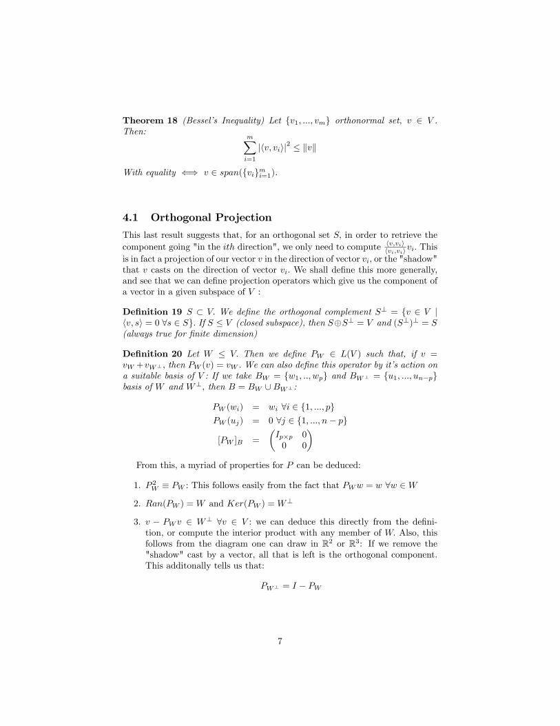
Theorem 18 (Bessel�s Inequality) Let fv1; :::; vmg orthonormal set, v 2 V .Then:

mXi=1

jhv; viij2 � kvk

With equality () v 2 span(fvigmi=1).

4.1 Orthogonal Projection

This last result suggests that, for an orthogonal set S; in order to retrieve thecomponent going "in the ith direction", we only need to compute hv;vii

hvi;viivi: Thisis in fact a projection of our vector v in the direction of vector vi; or the "shadow"that v casts on the direction of vector vi: We shall de�ne this more generally,and see that we can de�ne projection operators which give us the component ofa vector in a given subspace of V :

De�nition 19 S � V: We de�ne the orthogonal complement S? = fv 2 V jhv; si = 0 8s 2 Sg: If S � V (closed subspace), then S�S? = V and (S?)? = S(always true for �nite dimension)

De�nition 20 Let W � V: Then we de�ne PW 2 L(V ) such that, if v =vW +vW? ; then PW (v) = vW : We can also de�ne this operator by it�s action ona suitable basis of V : If we take BW = fw1; ::; wpg and BW? = fu1; :::; un�pgbasis of W and W?; then B = BW [BW? :

PW (wi) = wi 8i 2 f1; :::; pgPW (uj) = 0 8j 2 f1; :::; n� pg

[PW ]B =

�Ip�p 00 0

�From this, a myriad of properties for P can be deduced:

1. P 2W � PW : This follows easily from the fact that PWw = w 8w 2W

2. Ran(PW ) =W and Ker(PW ) =W?

3. v � PW v 2 W? 8v 2 V : we can deduce this directly from the de�ni-tion, or compute the interior product with any member of W: Also, thisfollows from the diagram one can draw in R2 or R3: If we remove the"shadow" cast by a vector, all that is left is the orthogonal component.This additonally tells us that:

PW? = I � PW

7

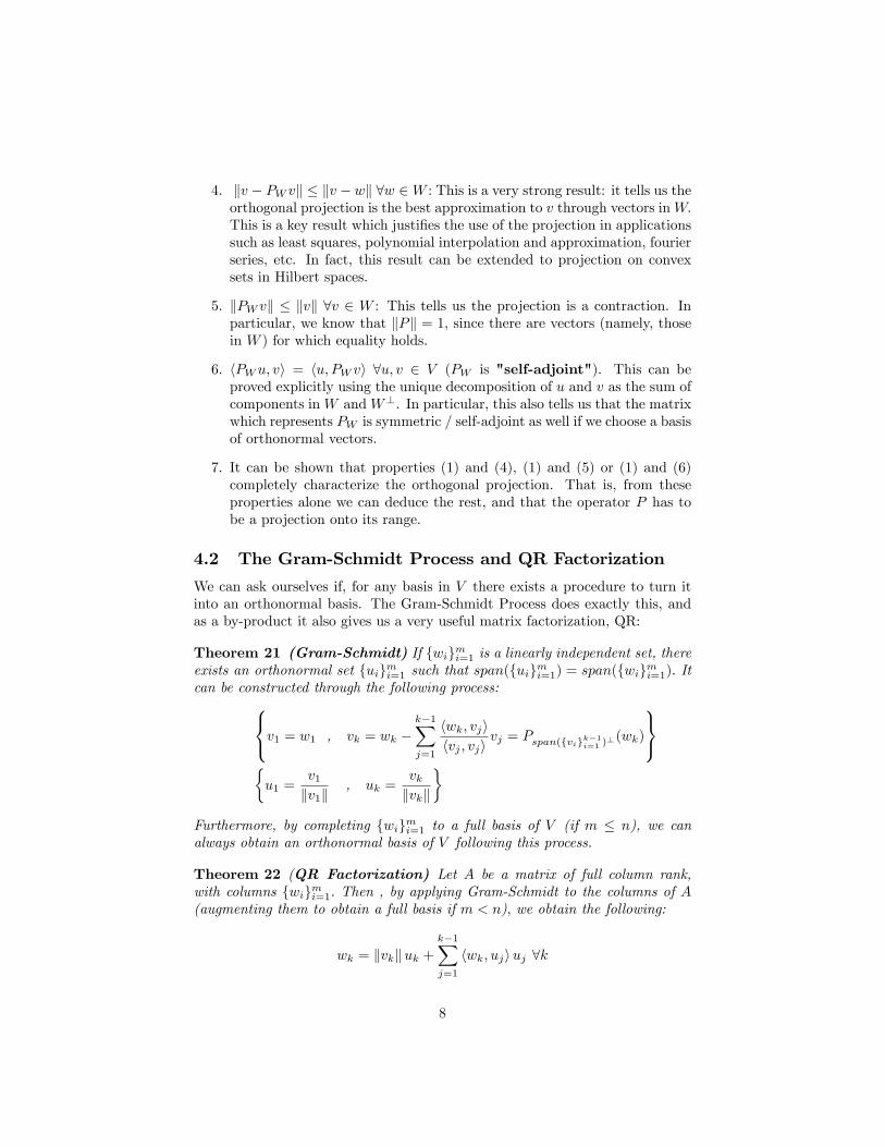
4. kv � PW vk � kv � wk 8w 2W : This is a very strong result: it tells us theorthogonal projection is the best approximation to v through vectors inW:This is a key result which justi�es the use of the projection in applicationssuch as least squares, polynomial interpolation and approximation, fourierseries, etc. In fact, this result can be extended to projection on convexsets in Hilbert spaces.

5. kPW vk � kvk 8v 2 W : This tells us the projection is a contraction. Inparticular, we know that kPk = 1; since there are vectors (namely, thosein W ) for which equality holds.

6. hPWu; vi = hu; PW vi 8u; v 2 V (PW is "self-adjoint"). This can beproved explicitly using the unique decomposition of u and v as the sum ofcomponents inW andW?. In particular, this also tells us that the matrixwhich represents PW is symmetric / self-adjoint as well if we choose a basisof orthonormal vectors.

7. It can be shown that properties (1) and (4), (1) and (5) or (1) and (6)completely characterize the orthogonal projection. That is, from theseproperties alone we can deduce the rest, and that the operator P has tobe a projection onto its range.

4.2 The Gram-Schmidt Process and QR Factorization

We can ask ourselves if, for any basis in V there exists a procedure to turn itinto an orthonormal basis. The Gram-Schmidt Process does exactly this, andas a by-product it also gives us a very useful matrix factorization, QR:

Theorem 21 (Gram-Schmidt) If fwigmi=1 is a linearly independent set, thereexists an orthonormal set fuigmi=1 such that span(fuigmi=1) = span(fwigmi=1): Itcan be constructed through the following process:8<:v1 = w1 , vk = wk �

k�1Xj=1

hwk; vjihvj ; vji

vj = Pspan(fvigk�1i=1 )?(wk)

9=;�u1 =

v1kv1k

, uk =vkkvkk

�Furthermore, by completing fwigmi=1 to a full basis of V (if m � n), we canalways obtain an orthonormal basis of V following this process.

Theorem 22 (QR Factorization) Let A be a matrix of full column rank,with columns fwigmi=1: Then , by applying Gram-Schmidt to the columns of A(augmenting them to obtain a full basis if m < n); we obtain the following:

wk = kvkkuk +k�1Xj=1

hwk; ujiuj 8k

8

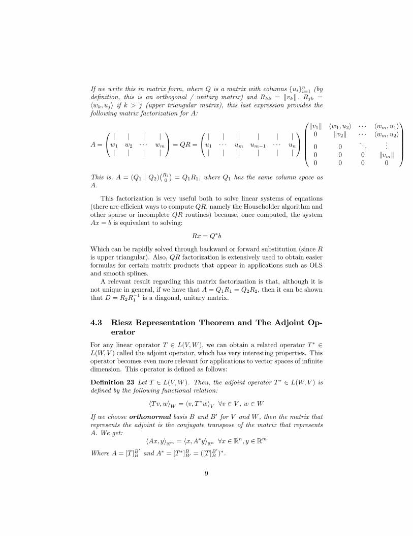
If we write this in matrix form, where Q is a matrix with columns fuigni=1 (byde�nition, this is an orthogonal / unitary matrix) and Rkk = kvkk ; Rjk =hwk; uji if k > j (upper triangular matrix), this last expression provides thefollowing matrix factorization for A:

A =

0@ j j j jw1 w2 � � � wmj j j j

1A = QR =

0@ j j j j j ju1 � � � um um�1 � � � unj j j j j j

1A0BBBBB@kv1k hw1; u2i � � � hwm; u1i0 kv2k � � � hwm; u2i

0 0. . .

...0 0 0 kvmk0 0 0 0

1CCCCCAThis is, A = (Q1 j Q2)

�R1

0

�= Q1R1, where Q1 has the same column space as

A.

This factorization is very useful both to solve linear systems of equations(there are e¢ cient ways to compute QR; namely the Householder algorithm andother sparse or incomplete QR routines) because, once computed, the systemAx = b is equivalent to solving:

Rx = Q�b

Which can be rapidly solved through backward or forward substitution (since Ris upper triangular). Also, QR factorization is extensively used to obtain easierformulas for certain matrix products that appear in applications such as OLSand smooth splines.A relevant result regarding this matrix factorization is that, although it is

not unique in general, if we have that A = Q1R1 = Q2R2, then it can be shownthat D = R2R

�11 is a diagonal, unitary matrix.

4.3 Riesz Representation Theorem and The Adjoint Op-erator

For any linear operator T 2 L(V;W ); we can obtain a related operator T � 2L(W;V ) called the adjoint operator, which has very interesting properties. Thisoperator becomes even more relevant for applications to vector spaces of in�nitedimension. This operator is de�ned as follows:

De�nition 23 Let T 2 L(V;W ). Then, the adjoint operator T � 2 L(W;V ) isde�ned by the following functional relation:

hTv;wiW = hv; T �wiV 8v 2 V , w 2W

If we choose orthonormal basis B and B0 for V and W , then the matrix thatrepresents the adjoint is the conjugate transpose of the matrix that representsA: We get:

hAx; yiRm = hx;A�yiRn 8x 2 Rn; y 2 Rm

Where A = [T ]B0

B and A� = [T �]BB0 = ([T ]B0

B )�.

9

The existence and uniqueness of this operator is given by the Riesz Repre-sentation Theorem for Hilbert Spaces:

Theorem 24 (Riesz Representation) Let V vs=F a Hilbert space, and T 2L(V; F ) a continuous, linear functional (element of the topological dual). Then,9!v 2 V such that:

Tu = hu; vi 8u 2 V

Therefore, the Adjoint operator is always well de�ned by the functionalrelation we have outlined, parting from the linear functional Lwv = hTv;wiW�xing each w 2W:

Remark 25 Here is a quick application of the adjoint operator and the orthog-onal projection operator: Let A 2 Mm�n(F ); and Ax = b a system of linearequations. Then the least squares solution to this system is given by the solutionto:

rrrrrrrrrrrrAx0 = PRan(A)(b)

Since we are projecting b onto the column space of A; and we know this is thebest approximation we can have using linear combinations of the columns of A:Using properties of the projection operator, we now know that:

Ax; b� PRan(A)(b)�= 0 8x

hAx; b�Ax0i = 0

Now, using the adjoint of A; we �nd:

hx;A�b�A�Ax0i = 0 8x

So, this means A�b = A�Ax0; and therefore, if A�A is invertible, this means

x0 = (A�A)�1A�bby = Ax0 = A(A�A)�1A�b

Incidentally, this also tells us that the projection matrix of a vector onto thecolumn space of a matrix A is given by PRan(A) = A(A�A)�1A�.

Properties of the Adjoint: (T 2 L(V;W ))

1. (T + S)� = T � + S�

2. (�T )� = �T �

3. (T �)� = T

4. I�V = IV (the identity is self-adjoint)

5. (ST )� = T �S�

10

6. B and B0 orthonormal basis of V and W () then [T �]BB0 = ([T ]B0

B )�

(be careful, this is an () statement)

The most important property of the adjoint, however, provides us with anexplicit relation between the kernel and the image of T and T �. These relationscan be deduced directly from the de�nition, and provide us with comprehensivetools to study spaces V and W:

Theorem 26 ("Fundamental Theorem of Linear Algebra II") Let V;W�nite dimentional Hilbert spaces, T 2 L(V;W ): Then:

Ker(T �) = Ran(T )?

Ran(T �) = Ker(T )?

Thus, we can always write V = Ker(T )�Ran(T �) andW = Ker(T �)�Ran(T ).

Proof. (Ker(T �) = Ran(T )?): Let v 2 Ker(T �); and any Tu 2 Ran(T ); thenv 2 Ran(T )? () hTu; vi = 0 8u () hu; T �vi = 0 8u () v 2 Ker(T �).The proof of the second statement can be found replacing T and T � above.

A couple of results that follow from this one are:

1. T is injective () T � is onto

2. Ker(T �T ) = Ker(T ), and thus, r(T �T ) = r(T ) = r(T �) (rank).

5 Normal and Self-Adjoint Operators: SpectralTheorems and Related Results

Depending on the �eld F we are working with, we can obtain "�eld sensitive"theorems that characterize diagonalizable operators. In particular, we are in-terested in the cases where the �eld is either R or C: This discussion will alsoyield important results on isometric, unitary and positive operators.

De�nition 27 T 2 L(V ) is said to be a self-adjoint operator if T � T �. IfF = R, this is equivalent to saying [T ]B is symmetric, and if F = C, that [T ]Bis Hermitian (equal to its conjugate transpose).

De�nition 28 T 2 L(V ) is said to be normal if it commutes with its adjoint,that is, if TT � = T �T:

Remark 29 If F = R, then an operator T is normal and it is not self-adjoint() 8B orthogonal basis of V , [T ]B is a block diagonal matrix, with blocks ofsize 1 and blocks of size 2 which are multiples of rotation matrices.

First, we introduce a couple of interesting results on self-adjoint and normaloperators:

11

Proposition 30 T 2 L(V ); F = C then there exist unique self-adjoint opera-tors T1 and T2 such that T = T1 + iT2: T is then self-adjoint () T2 � 0, andis normal () T1T2 = T2T1: These operators are given by:

T1 =T + T �

2, T2 =

T � T �2i

Proposition 31 If T 2 L(V ) is normal, then Ker(T ) = Ker(T �) and Ran(T ) =Ran(T �):

The most important properties of these families of operators, however, haveto do with the spectral information we can retrieve:

Proposition 32 T 2 L(V ) and self-adjoint and F = C: If � is an eigenvalueof T , then � 2 R

Proof. For u eigenvector, we have:

� hu; ui = hu; Tui = hTu; ui = � hu; ui� = �

Proposition 33 T 2 L(V ) and F = C: T is self-adjoint () hTv; vi 2 R8v 2 V

Proof. Using both self-adjoint and properties of the interior product:

hTv; vi = hv; Tvi = hTv; vi 8v 2 V

This, in particular tells us the Rayleigh quotient for such an operator isalways real, and we can also rederive last proposition.

Proposition 34 If T 2 L(V ) is a normal operator,i) kTvk = kT �vk 8v 2 Vii) T � I is normal 8 2 Ciii) v is an eigenvector of T () v is an eigenvector of T �

Proof. (i): hTv; Tvi = hv; T �Tvi = hv; TT �vi = hT �v; T �vi(ii): (T � I)�(T � I) = T �T � I(T +T �)+ 2I = TT �� I(T �+T )+ 2I =(T � I)(T � I)�(iii): (T � �I)v = 0 =) k(T � �I)�vk = 0 (by i and ii) () (T � �I)�v = 0

12

Theorem 35 (Spectral Theorem, F = C Version) V vs=C �nite dimen-tional Hilbert space. T 2 L(V ). V has an orthonormal basis of eigenvectors ofT () T is normal.

Proof. ((=) By Schur�s factorization, there exists a basis of V such that [T ]B isupper triangular. By Gram-Schmidt, I can turn this basis into an orthonormalone Q, and by studying the QR factorization, we realize the resulting matrixis still upper triangular. However, since the basis is now orthonormal, andT is normal, it follows that [T ]Q is a normal, upper triangular matrix. Thisnecessarily implies [T ]S is diagonal (We can see this by computing the productsof the o¤-diagonal elements, and concluding they have to be zero in order forthis to hold).(=)) If this is the case, then we have Q an orthonormal basis and � diagonal

such that [T ]Q = �: Since a diagonal matrix is always normal, it follows that Tis a normal operator.

Theorem 36 (Spectral Theorem, F = R Version) V vs=R �nite dimen-tional Hilbert space. T 2 L(V ). V has an orthonormal basis of eigenvectors ofT () T is self-adjoint.

Proof. We follow the proof for the complex case, noting that, since F = R; bothSchur�s factorization and Gram-Schmidt will yield matrices with real entries.Finally a diagonal matrix with real entries is always self-adjoint (since this onlymeans that it is symmetric). We can also apply the theorem for the complexcase and use the properties for self-adjoint operators.

In any case, we then have the following powerful properties:

1. V =kMi=1

E�i and (E�i)? =

Mj 6=i

E�j 8i

2. If we denote Pj = PE�j , then PiPj = �ij

3. (Spectral Resolution of Identity)

IV =kXi=1

Pi

4. (Spectral Resolution of T )

T =kXi=1

�iPi

These properties characterize all diagonalizable operators on �nite dimen-sional Hilbert spaces. Some important results that follow from this are:

13

Theorem 37 (Cayley-Hamilton) T 2 L(V ); V �nite dimensional Hilbert space.If p is the characteristic polynomial of T; then p(T ) � 0.

Theorem 38 V vs=C and T 2 L(V ) normal, then 9p 2 C[x] polynomial suchthat p(T ) = T �. This polynomial can be found by the Lagrange Interpolationproblem fp(�i) = �igki=1

We also have the following properties for T normal, which we can now deduceusing the spectral decomposition of T . These properties basically tell us that, ifT is normal, we can operate it almost as if it were a number through its spectralrepresentation.

1. If q is a polynomial, then q(T ) =Pk

i=1 q(�i)Pi

2. If T p � 0 for some p, then T � 0

3. An operator commutes with T () it commutes with each Pi

4. T has a normal "square root" (S such that S2 = T )

5. T is a projection () all its eigenvalues are 00s or 10s:

6. T = �T � (anti-adjoint) () all eigenvalues are pure imaginary numbers

5.1 Unitary Operators

De�nition 39 An operator T 2 L(V ) is said to be orthogonal (R) / unitary(C) if kTvk = kvk 8v 2 V (this means T is a linear isometry, it is a "rigidtransformation"). A unitary operator can also be characterized by T normaland T �T = TT � = IV :

Theorem 40 (Mazur-Ulam) If f is an isometry such that f(0) = 0 and f isonto, then f is a linear isometry (unitary operator)

Theorem 41 The following statements are equivalent for T 2 L(V ) :i) T is an isometryii) T �T = TT � = IViii) hTu; Tvi = hu; vi 8u; v 2 Viv) If B is an orthonormal basis, T (B) is an orthonormal basisv) There exists an orthonormal basis of V such that T (B) is an orthonormalbasis.

Theorem 42 If � is an eigenvalue of an isometry, then j�j = 1. T is then anisometry () T � is an isometry as well.

14

5.2 Positive Operators and Square Roots

De�nition 43 V a �nite dimensional Hilbert Space, T 2 L(V ). We say T isa positive operator if T is self-adjoint and hTv; vi � 0 8v 2 V

Remark 44 A matrix A is said to be a positive operator (positive semide�nitematrix) if hAx; xi = x>Ax � 0 8x 2 Fn

Remark 45 If F = C, we can remove the assumption that T is self-adjoint.

Remark 46 The operators T �T and TT � are always positive. In fact, it canbe shown any positive operator T is of the form SS�: This is a general versionof the famous Cholesky factorization for symmetric positive de�nite matrices.

Proposition 47 T is a positive operator () T is self-adjoint and all itseigenvalues are real and non-negative.

Some properties of positive operators:

1. T;U 2 L(V ) positive operators, then T + U is positive

2. T 2 L(V ) is positive =) cT is positive 8c � 0

3. T 2 L(V ) is positive and invertible =) T�1 is positive

4. T 2 L(V ) positive =) T 2 is positive (the converse is false in general)

5. T;U 2 L(V ) positive operators, then TU = UT implies TU is positive.Here we use heavily that TU = UT implies there is a basis of vectorswhich are simultaneously eigenvectors of T and U:

De�nition 48 T 2 L(V ): Then we say S is a square root of T if S2 = T .

We note that, in general, the square root is not unique, For example, theidentity has an in�nite number of square roots: permutations, re�ections androtations by 180�: However, we can show that, if an operator is positive, thenit has a unique positive square root.

Proposition 49 T 2 L(V ) is positive () T has a unique positive squareroot.

15

6 Singular Value Decomposition and theMoore-Penrose Generalized Inverse

6.1 Singular Value Decomposition

The Singular Value Decomposition for T 2 L(V;W ) (and the correspondingfactorization for matrices) is, without a doubt, one of the most useful resultsin linear algebra. It is used in applications such as Least Squares Regression,Smooth Spline and Ridge Regression, Principal Component Analysis, MatrixNorms, Noise Filtering, Low Rank approximation of matrices and operators,etc. This decomposition also enables us to de�ne a generalized inverse (alsoknown as the pseudoinverse), and to compute other decompositions, such as thePolar decomposition for positive operators and computing positive square rootsexplicitly.

Theorem 50 (Singular Value Decomposition, or SVD) Let V;W vs=F Hilbertspaces, T 2 L(V;W ) with rank r. Then, there exist orthonormal basis of V andW fv1; ::; vng and fu1; ::; umg, as well as positive scalars �1 � �2 � ::: � �r > 0such that:

Tvi = �iui ; i � rTvi = 0 ; i > r

These scalars are called the "singular values" of T . Conversely, if basis andscalars like these exist, then fv1; ::; vng is an orthonormal basis of eigenvectorsof T �T such that the �rst r are associated to the eigenvalues �21; :::; �

2r, and the

rest are associated to � = 0.

Using what we know about positive operators, we can see how the state-ment of this theorem must always be true. Regardless of what T is, T �T isa positive operator, and therefore diagonalizable, with nonnegative eigenval-ues f�21; :::; �2rg and possibly also 0: Then, we obtain the set of fu1; ::; umg bycomputing Tvi=�i = ui for the �rst r vectors, and then completing it to anorthonormal basis of W .Also, this theorem immediately has a geometric interpretation: by choosing

the "right" basis, we know exactly what is the action of T on the unit sphere.Basically, T sends the unit sphere to the boundary of a r dimensional ellipsoid(since it squashes fvr+1; ::; vng to zero), with axis on the �rst r u0is: Also, thebiggest axis of this ellipsoid is the one in the direction of u1; and the smallestis the one in the direction of ur.Finally, we note that this theorem applied to a matrix A 2Mm�n(F ) yields

the following matrix factorization: If V;U are unitary matrices with fv1; ::; vngand fu1; ::; umg as columns, and if � is the matrix in Mm�n(F ) with all zeros

16

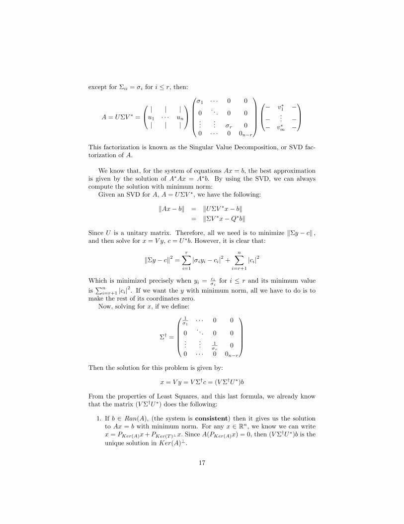
except for �ii = �i for i � r, then:

A = U�V � =

0@ j j ju1 � � � unj j j

1A0BBBB@�1 � � � 0 0

0. . . 0 0

...... �r 0

0 � � � 0 0n�r

1CCCCA0B@� v�1 �

�... �

� v�m �

1CAThis factorization is known as the Singular Value Decomposition, or SVD fac-torization of A:

We know that, for the system of equations Ax = b, the best approximationis given by the solution of A�Ax = A�b. By using the SVD, we can alwayscompute the solution with minimum norm:Given an SVD for A; A = U�V �, we have the following:

kAx� bk = kU�V �x� bk= k�V �x�Q�bk

Since U is a unitary matrix. Therefore, all we need is to minimize k�y � ck ;and then solve for x = V y, c = U�b: However, it is clear that:

k�y � ck2 =rXi=1

j�iyi � cij2 +nX

i=r+1

jcij2

Which is minimized precisely when yi = ci�ifor i � r and its minimum value

isPn

i=r+1 jcij2. If we want the y with minimum norm, all we have to do is to

make the rest of its coordinates zero.Now, solving for x; if we de�ne:

�y =

0BBBB@1�1

� � � 0 0

0. . . 0 0

...... 1

�r0

0 � � � 0 0n�r

1CCCCAThen the solution for this problem is given by:

x = V y = V �yc = (V �yU�)b

From the properties of Least Squares, and this last formula, we already knowthat the matrix (V �yU�) does the following:

1. If b 2 Ran(A), (the system is consistent) then it gives us the solutionto Ax = b with minimum norm. For any x 2 Rn; we know we can writex = PKer(A)x+PKer(T )?x: Since A(PKer(A)x) = 0; then (V �yU�)b is theunique solution in Ker(A)?.

17

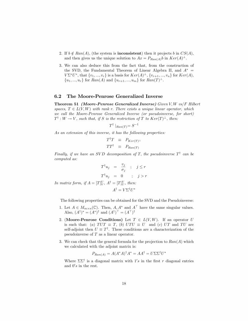
2. If b =2 Ran(A); (the system is inconsistent) then it projects b in CS(A);and then gives us the unique solution to Ax = PRan(A)b in Ker(A)?:

3. We can also deduce this from the fact that, from the construction ofthe SVD, the Fundamental Theorem of Linear Algebra II, and A� =V ��U�; that fv1; :::; vrg is a basis for Ker(A)?; fvr+1; :::; vng for Ker(A),fu1; :::; urg for Ran(A) and fur+1; :::; umg for Ran(T )?.

6.2 The Moore-Penrose Generalized Inverse

Theorem 51 (Moore-Penrose Generalized Inverse) Given V;W vs=F Hilbertspaces, T 2 L(V;W ) with rank r: There exists a unique linear operator, whichwe call the Moore-Penrose Generalized Inverse (or pseudoinverse, for short)T y :W ! V , such that, if S is the restriction of T to Ker(T )?, then:

T y jRan(T )= S�1

As an extension of this inverse, it has the following properties:

T yT � PKer(T )?

TT y � PRan(T )

Finally, if we have an SV D decomposition of T; the pseudoinverse T y can becomputed as:

T yuj =vj�j

; j � r

T yuj = 0 ; j > r

In matrix form, if A = [T ]UV , Ay = [T ]VU , then:

Ay = V �yU�

The following properties can be obtained for the SVD and the Pseudoinverse:

1. Let A 2 Mm�n(C). Then, A;A� and A> have the same singular values.Also, (Ay)� = (A�)y and (Ay)> = (A>)y

2. (Moore-Penrose Conditions) Let T 2 L(V;W ). If an operator Uis such that: (a) TUT � T , (b) UTU � U and (c) UT and TU areself-adjoint then U � T y. These conditions are a characterization of thepseudoinverse of T as a linear operator.

3. We can check that the general formula for the projection to Ran(A) whichwe calculated with the adjoint matrix is:

PRan(A) = A(A�A)yA� = AAy = U��yU�

Where ��y is a diagonal matrix with 10s in the �rst r diagonal entriesand 00s in the rest.

18

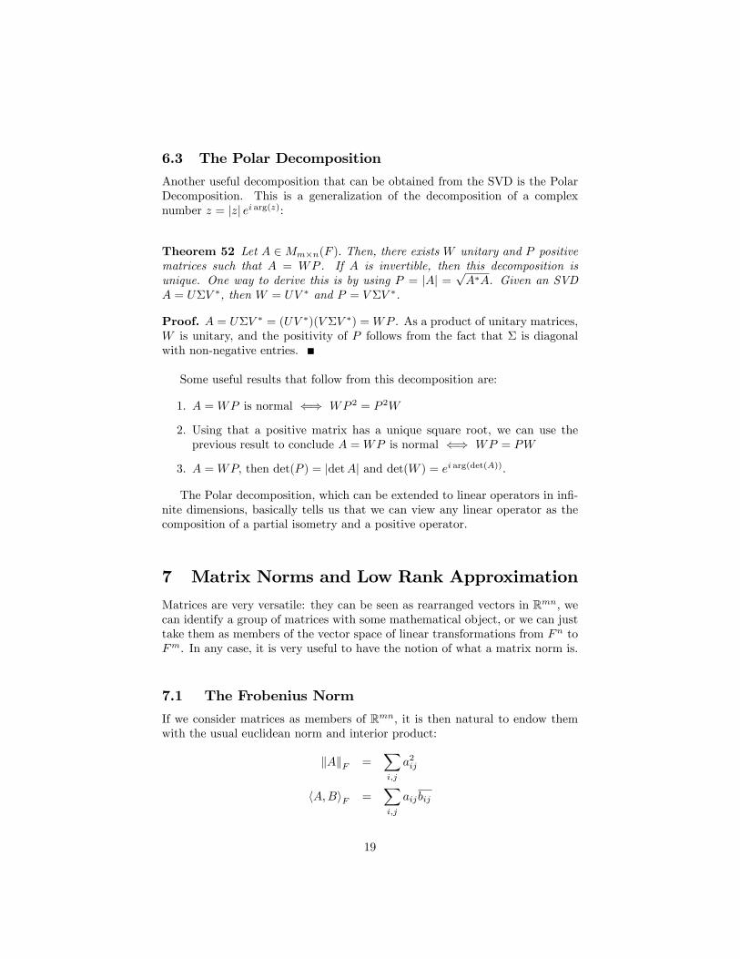
6.3 The Polar Decomposition

Another useful decomposition that can be obtained from the SVD is the PolarDecomposition. This is a generalization of the decomposition of a complexnumber z = jzj ei arg(z):

Theorem 52 Let A 2Mm�n(F ): Then, there exists W unitary and P positivematrices such that A = WP . If A is invertible, then this decomposition isunique. One way to derive this is by using P = jAj =

pA�A. Given an SVD

A = U�V �, then W = UV � and P = V �V �.

Proof. A = U�V � = (UV �)(V �V �) =WP . As a product of unitary matrices,W is unitary, and the positivity of P follows from the fact that � is diagonalwith non-negative entries.

Some useful results that follow from this decomposition are:

1. A =WP is normal () WP 2 = P 2W

2. Using that a positive matrix has a unique square root, we can use theprevious result to conclude A =WP is normal () WP = PW

3. A =WP; then det(P ) = jdetAj and det(W ) = ei arg(det(A)).

The Polar decomposition, which can be extended to linear operators in in�-nite dimensions, basically tells us that we can view any linear operator as thecomposition of a partial isometry and a positive operator.

7 Matrix Norms and Low Rank Approximation

Matrices are very versatile: they can be seen as rearranged vectors in Rmn, wecan identify a group of matrices with some mathematical object, or we can justtake them as members of the vector space of linear transformations from Fn toFm. In any case, it is very useful to have the notion of what a matrix norm is.

7.1 The Frobenius Norm

If we consider matrices as members of Rmn; it is then natural to endow themwith the usual euclidean norm and interior product:

kAkF =Xi;j

a2ij

hA;BiF =Xi;j

aijbij

19

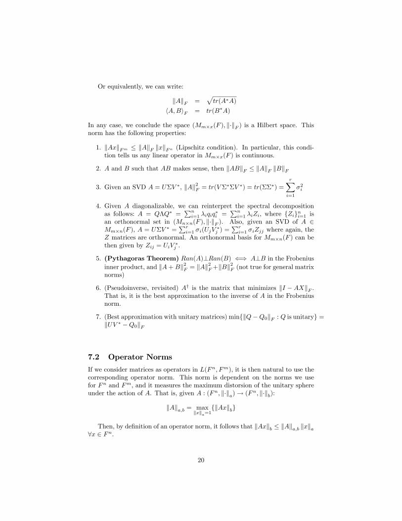
Or equivalently, we can write:

kAkF =ptr(A�A)

hA;BiF = tr(B�A)

In any case, we conclude the space (Mm�x(F ); k�kF ) is a Hilbert space. Thisnorm has the following properties:

1. kAxkFm � kAkF kxkFn (Lipschitz condition). In particular, this condi-tion tells us any linear operator in Mm�x(F ) is continuous.

2. A and B such that AB makes sense, then kABkF � kAkF kBkF

3. Given an SVD A = U�V �, kAk2F = tr(V ���V �) = tr(���) =rXi=1

�2i

4. Given A diagonalizable, we can reinterpret the spectral decompositionas follows: A = Q�Q� =

Pni=1 �iqiq

�i =

Pni=1 �iZi; where fZigni=1 is

an orthonormal set in (Mn�n(F ); k�kF ). Also, given an SVD of A 2Mm�n(F ); A = U�V

� =Pr

i=1 �i(UjV�j ) =

Pri=1 �iZjj where again, the

Z matrices are orthonormal. An orthonormal basis for Mm�n(F ) can bethen given by Zij = UiV �j .

5. (Pythagoras Theorem) Ran(A)?Ran(B) () A?B in the Frobeniusinner product, and kA+Bk2F = kAk

2F+kBk

2F (not true for general matrix

norms)

6. (Pseudoinverse, revisited) Ay is the matrix that minimizes kI �AXkF .That is, it is the best approximation to the inverse of A in the Frobeniusnorm.

7. (Best approximation with unitary matrices)minfkQ�Q0kF : Q is unitaryg =kUV � �Q0kF

7.2 Operator Norms

If we consider matrices as operators in L(Fn; Fm); it is then natural to use thecorresponding operator norm. This norm is dependent on the norms we usefor Fn and Fm, and it measures the maximum distorsion of the unitary sphereunder the action of A. That is, given A : (Fn; k�ka)! (Fn; k�kb):

kAka;b = maxkxka=1

fkAxkbg

Then, by de�nition of an operator norm, it follows that kAxkb � kAka;b kxka8x 2 Fn.

20

This maximum is always attained at some point in the sphere, since kAxkb isa continuous function, and the sphere is compact. Although we can potentiallyuse any norms we want on the domain and range of the transformation, it isoften the case that k�ka and k�kb are both p-norms with the same value of p: Inthis case, we talk about the p� norm of A as kAkp;p.An important question that arises then is how to calculate this operator

norm. For a general p, this becomes a constrained optimization problem (oftena nontrivial one for general p). However, for some important cases, we can againsay something in terms of the SVD or in terms of the entries of A.

Properties of kAk2 :

1. kAk2 = maxf�ig = �1 : As we know, this is a very signi�cant fact, thatis deeply tied with the geometrical interpretation of the SVD. As it wasmentioned before, the SVD reveals that the sphere is mapped to an rdimensional ellipsoid, where the major axis has length �1.

2. minfkAxk2 : x 2 Ran(A�),kxk2 = 1g = �r

3. kAk2 = maxkxk2=1

f maxkyk2=1

fy�Axgg = maxkxk2=1

f maxkyk2=1

fhAx; yiFmgg

4. kAk2 = kA�Ak2 = kA�k25. For U and V unitary, kU�AV k2 = kAk26. A invertible, then

A�1 2= 1

�r. In general, we have

Ay 2= 1

�r.

We also have a result for the 1 and 1 norms:

kAk1 = maxj=1;::;m

fnXi=1

jaij jg (maximum of k�k1 norm of columns)

kAk1 = maxi=1;::;n

fmXj=1

jaij jg (maximum of k�k1 norm of rows)

We observe that kAk1 = kA�k1.

7.3 Low Rank Matrix Approximation:

We have now seen that the SVD provides us with tools to compute matrixnorms and to derive results of the vector space of matrices of a certain size. Ina way that is completely analogous to the theory of general Hilbert spaces, thisleads us to a theory of matrix approximation, by eliminating the singular valuesthat are not signi�cant and therefore producing an approximation of A that has

21

lower rank. This can immediately be seen as truncating a "Fourier Series" ofA; using the orthonormal basis that is suggested by our SVD:Let A = U�V � =

Pri=1 �i(UiV

�i ) =

Pri=1 �iZii, where fZijg = fUiV �j g

is the orthonormal basis of Mm�n(F ) (with respect to the Frobenius interiorproduct) as before. Then, it becomes evident that:

�i = hA;ZiiiFThat is, the �i (and all of the entries in �) are the Fourier coe¢ cients of A usingthis particular orthonormal basis. We notice that, since the Zij are exteriorproducts of two vectors, it follows that rank(Zij) = 1 8i; j.Now, it is often the case that A will be "noisy", either because it represents

the pixels in a blurred image, or because it is a transformation that involves somenoise. However, as in other instances of �ltering or approximation schemes, weexpect the noise to be of "high frequency", or equivalently, we know that thesignal to noise ratio decreases in proportion to �i. Therefore, by truncating theseries after a certain �k; the action of A remains almost intact, but we often getrid of a signi�cant amount of "noise". Also, using results of abstract Fourierseries, we can derive the fact that this is the best approximation to A of rank kin the Frobenius norm, that is:

Ak =kXi=1

�iZii

kA�Akk2F =

kXi=1

�2i = minrank(B)=k

fkA�Bk2F g

We also have the following results:

1. De�ning the "error matrix" Ek = A� Ak, it follows by Pythagoras The-orem that kAkk2F = kAk

2F � kEkk

2F : We can also de�ne a relative error,

or

R2k =kEkk2FkAk2F

=

Pri=k+1 �

2iPr

i=1 �2i

2. The matrix Ak is the result of k succesive approximations to A; each ofrank 1.

3. Ak is also an optimal approximation under the k�k2 norm, with minimumvalue �k+1.

8 Generalized Eigenvalues, the Jordan Canoni-cal Form and eA

The theory of generalized eigenspaces is a natural extension of the results fordiagonalizable operators and their spectral decomposition. Although the SVD

22

does provide some of these properties, it is desireable to have a decompositionof the space as the orthogonal sum of invariant subspaces. This also leads tothe Jordan Canonical form, which is a block diagonal matrix with which wecan easily operate and calculate matrix powers, power series and importantoperators like the exponential operator.

8.1 The Generalized Eigenspace K�

De�nition 53 Let V be a vector space over C, T 2 L(V ). For � eigenvalueof T; we de�ne am(�) the algebraic multiplicity as the multiplicity of the root� of the characteristic polynomial p(�) = det(T � �I) and gm(�) the geometricmultiplicity as the dimension of the eigenspace E� = Ker(T � �I).

Let V be a vector space over C, T 2 L(V ) a linear operator. We knowthat T has a set of distinct eigenvalues f�igki=1 and it is either the case that thealgebraic and the geometric multiplicity of each �i coincide (T is diagonalizable)or that, for some �; gm(�) < am(�). In the latter case, the problem is that theeigenspaces fail to span the entire space. We can then consider powers of theoperator (T � �I); and since Ker((T � �I)m) � Ker((T � �I)m+1) 8m (thespace "grows"), we can de�ne the following:

K� = fv 2 V : (T � �I)mv = 0 for some m 2 Ng

These generalized eigenspaces have the following properties:

1. E� � K� 8� eigenvalue of T (by de�nition)

2. K� � V and is invariant under the action of T : T (K�) � K�

3. If dim(V ) <1 then dim(K�) = am(�)

4. K�1 \K�2 = ? for �1 6= �2

Theorem 54 (Generalized Eigenvector Decomposition) Let V be a vectorspace over C, T 2 L(V ). Then if f�igki=1 are the eigenvalues of T and thecharacteristic polynomial p(�) splits in the �eld F ,

V =kMi=1

K�i

Proof.

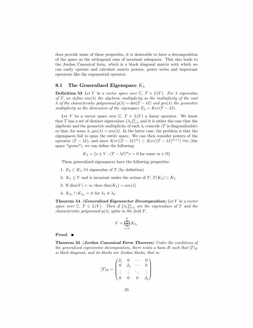
Theorem 55 (Jordan Canonical Form Theorem) Under the conditions ofthe generalized eigenvector decomposition, there exists a basis B such that [T ]Bis block diagonal, and its blocks are Jordan blocks, that is:

[T ]B =

0BBB@J1 0 � � � 00 J2 � � � 0...

.... . .

...0 0 0 Jk

1CCCA23

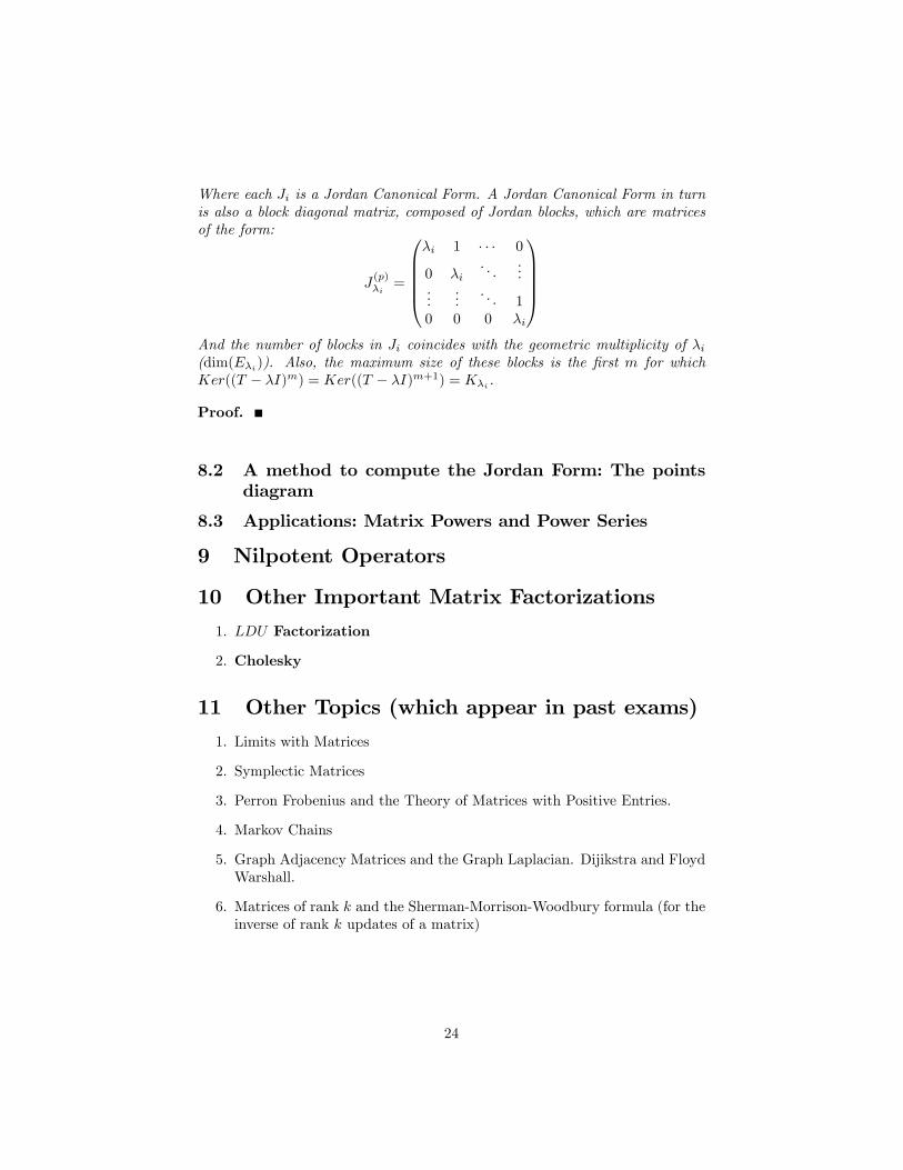
Where each Ji is a Jordan Canonical Form. A Jordan Canonical Form in turnis also a block diagonal matrix, composed of Jordan blocks, which are matricesof the form:

J(p)�i=

0BBBB@�i 1 � � � 0

0 �i. . .

......

.... . . 1

0 0 0 �i

1CCCCAAnd the number of blocks in Ji coincides with the geometric multiplicity of �i(dim(E�i)). Also, the maximum size of these blocks is the �rst m for whichKer((T � �I)m) = Ker((T � �I)m+1) = K�i .

Proof.

8.2 A method to compute the Jordan Form: The pointsdiagram

8.3 Applications: Matrix Powers and Power Series

9 Nilpotent Operators

10 Other Important Matrix Factorizations

1. LDU Factorization

2. Cholesky

11 Other Topics (which appear in past exams)

1. Limits with Matrices

2. Symplectic Matrices

3. Perron Frobenius and the Theory of Matrices with Positive Entries.

4. Markov Chains

5. Graph Adjacency Matrices and the Graph Laplacian. Dijikstra and FloydWarshall.

6. Matrices of rank k and the Sherman-Morrison-Woodbury formula (for theinverse of rank k updates of a matrix)

24

12 Yet more Topics I can think of

1. Symmetric Positive Semide�nite Matrices and the Variance CovarianceMatrix

2. Krylov Subspaces: CG, GMRES and Lanczos Algorithms

3. Toeplitz and Wavelet Matrices

4. Polynomial Interpolation

25