linear algebra. vector calculus · linear algebra: matrices, vectors, determinants. linear systems...
TRANSCRIPT

C H A P T E R 7 Linear Algebra: Matrices, Vectors, Determinants. Linear Systems
C H A P T E R 8 Linear Algebra: Matrix Eigenvalue Problems
C H A P T E R 9 Vector Differential Calculus. Grad, Div, Curl
C H A P T E R 1 0 Vector Integral Calculus. Integral Theorems
255
P A R T B
Linear Algebra.Vector Calculus
Matrices and vectors, which underlie linear algebra (Chaps. 7 and 8), allow us to representnumbers or functions in an ordered and compact form. Matrices can hold enormous amountsof data—think of a network of millions of computer connections or cell phone connections—in a form that can be rapidly processed by computers. The main topic of Chap. 7 is howto solve systems of linear equations using matrices. Concepts of rank, basis, lineartransformations, and vector spaces are closely related. Chapter 8 deals with eigenvalueproblems. Linear algebra is an active field that has many applications in engineeringphysics, numerics (see Chaps. 20–22), economics, and others.
Chapters 9 and 10 extend calculus to vector calculus. We start with vectors from linearalgebra and develop vector differential calculus. We differentiate functions of severalvariables and discuss vector differential operations such as grad, div, and curl. Chapter 10extends regular integration to integration over curves, surfaces, and solids, therebyobtaining new types of integrals. Ingenious theorems by Gauss, Green, and Stokes allowus to transform these integrals into one another.
Software suitable for linear algebra (Lapack, Maple, Mathematica, Matlab) can be foundin the list at the opening of Part E of the book if needed.
Numeric linear algebra (Chap. 20) can be studied directly after Chap. 7 or 8 becauseChap. 20 is independent of the other chapters in Part E on numerics.

256
C H A P T E R 7
Linear Algebra: Matrices,Vectors, Determinants. Linear Systems
Linear algebra is a fairly extensive subject that covers vectors and matrices, determinants,systems of linear equations, vector spaces and linear transformations, eigenvalue problems,and other topics. As an area of study it has a broad appeal in that it has many applicationsin engineering, physics, geometry, computer science, economics, and other areas. It alsocontributes to a deeper understanding of mathematics itself.
Matrices, which are rectangular arrays of numbers or functions, and vectors are themain tools of linear algebra. Matrices are important because they let us express largeamounts of data and functions in an organized and concise form. Furthermore, sincematrices are single objects, we denote them by single letters and calculate with themdirectly. All these features have made matrices and vectors very popular for expressingscientific and mathematical ideas.
The chapter keeps a good mix between applications (electric networks, Markovprocesses, traffic flow, etc.) and theory. Chapter 7 is structured as follows: Sections 7.1and 7.2 provide an intuitive introduction to matrices and vectors and their operations,including matrix multiplication. The next block of sections, that is, Secs. 7.3–7.5 providethe most important method for solving systems of linear equations by the Gausselimination method. This method is a cornerstone of linear algebra, and the methoditself and variants of it appear in different areas of mathematics and in many applications.It leads to a consideration of the behavior of solutions and concepts such as rank of amatrix, linear independence, and bases. We shift to determinants, a topic that hasdeclined in importance, in Secs. 7.6 and 7.7. Section 7.8 covers inverses of matrices.The chapter ends with vector spaces, inner product spaces, linear transformations, andcomposition of linear transformations. Eigenvalue problems follow in Chap. 8.
COMMENT. Numeric linear algebra (Secs. 20.1–20.5) can be studied immediatelyafter this chapter.
Prerequisite: None.Sections that may be omitted in a short course: 7.5, 7.9.References and Answers to Problems: App. 1 Part B, and App. 2.

7.1 Matrices, Vectors: Addition and Scalar Multiplication
The basic concepts and rules of matrix and vector algebra are introduced in Secs. 7.1 and7.2 and are followed by linear systems (systems of linear equations), a main application,in Sec. 7.3.
Let us first take a leisurely look at matrices before we formalize our discussion. A matrixis a rectangular array of numbers or functions which we will enclose in brackets. For example,
(1)
are matrices. The numbers (or functions) are called entries or, less commonly, elementsof the matrix. The first matrix in (1) has two rows, which are the horizontal lines of entries.Furthermore, it has three columns, which are the vertical lines of entries. The second andthird matrices are square matrices, which means that each has as many rows as columns—3 and 2, respectively. The entries of the second matrix have two indices, signifying theirlocation within the matrix. The first index is the number of the row and the second is thenumber of the column, so that together the entry’s position is uniquely identified. Forexample, (read a two three) is in Row 2 and Column 3, etc. The notation is standardand applies to all matrices, including those that are not square.
Matrices having just a single row or column are called vectors. Thus, the fourth matrixin (1) has just one row and is called a row vector. The last matrix in (1) has just onecolumn and is called a column vector. Because the goal of the indexing of entries wasto uniquely identify the position of an element within a matrix, one index suffices forvectors, whether they are row or column vectors. Thus, the third entry of the row vectorin (1) is denoted by
Matrices are handy for storing and processing data in applications. Consider thefollowing two common examples.
E X A M P L E 1 Linear Systems, a Major Application of Matrices
We are given a system of linear equations, briefly a linear system, such as
where are the unknowns. We form the coefficient matrix, call it A, by listing the coefficients of theunknowns in the position in which they appear in the linear equations. In the second equation, there is nounknown which means that the coefficient of is 0 and hence in matrix A, Thus,a22 � 0,x2x2,
x1, x2, x3
4x1 � 6x2 � 9x3 � 6
6x1 � 2x3 � 20
5x1 � 8x2 � x3 � 10
a3.
a23
c e�x 2x2
e6x 4xd , [a1 a2 a3], c4
12
d
c0.3 1 �5
0 �0.2 16d , Da11 a12 a13
a21 a22 a23
a31 a32 a33
T ,
SEC. 7.1 Matrices, Vectors: Addition and Scalar Multiplication 257

by augmenting A with the right sides of the linear system and call it the augmented matrix of the system.Since we can go back and recapture the system of linear equations directly from the augmented matrix ,
contains all the information of the system and can thus be used to solve the linear system. This means that wecan just use the augmented matrix to do the calculations needed to solve the system. We shall explain this indetail in Sec. 7.3. Meanwhile you may verify by substitution that the solution is .
The notation for the unknowns is practical but not essential; we could choose x, y, z or some otherletters.
E X A M P L E 2 Sales Figures in Matrix Form
Sales figures for three products I, II, III in a store on Monday (Mon), Tuesday (Tues), may for each weekbe arranged in a matrix
If the company has 10 stores, we can set up 10 such matrices, one for each store. Then, by adding correspondingentries of these matrices, we can get a matrix showing the total sales of each product on each day. Can you thinkof other data which can be stored in matrix form? For instance, in transportation or storage problems? Or inlisting distances in a network of roads?
General Concepts and NotationsLet us formalize what we just have discussed. We shall denote matrices by capital boldfaceletters A, B, C, , or by writing the general entry in brackets; thus , and soon. By an matrix (read m by n matrix) we mean a matrix with m rows and ncolumns—rows always come first! is called the size of the matrix. Thus an matrix is of the form
(2)
The matrices in (1) are of sizes and respectively.Each entry in (2) has two subscripts. The first is the row number and the second is the
column number. Thus is the entry in Row 2 and Column 1.If we call A an square matrix. Then its diagonal containing the entries
is called the main diagonal of A. Thus the main diagonals of the twosquare matrices in (1) are and respectively.
Square matrices are particularly important, as we shall see. A matrix of any size is called a rectangular matrix; this includes square matrices as a special case.
m � ne�x, 4x,a11, a22, a33
a11, a22, Á , ann
n � nm � n,a21
2 � 1,2 � 3, 3 � 3, 2 � 2, 1 � 3,
A � 3ajk4 � Ea11 a12Á a1n
a21 a22Á a2n
# # Á #
am1 am2Á amn
U .
m � nm � nm � n
A � [ajk]Á
�
A �
Mon Tues Wed Thur Fri Sat Sun
40 33 81 0 21 47 33D 0 12 78 50 50 96 90 T10 0 0 27 43 78 56
# I
II
III
Á
�x1, x2, x3
x1 � 3, x2 � 12, x3 � �1
A~
A~
A � D4 6 9
6 0 �2
5 �8 1
T . We form another matrix A~
� D4 6 9 6
6 0 �2 20
5 �8 1 10
T258 CHAP. 7 Linear Algebra: Matrices, Vectors, Determinants. Linear Systems

VectorsA vector is a matrix with only one row or column. Its entries are called the componentsof the vector. We shall denote vectors by lowercase boldface letters a, b, or by itsgeneral component in brackets, , and so on. Our special vectors in (1) suggestthat a (general) row vector is of the form
A column vector is of the form
Addition and Scalar Multiplication of Matrices and VectorsWhat makes matrices and vectors really useful and particularly suitable for computers isthe fact that we can calculate with them almost as easily as with numbers. Indeed, wenow introduce rules for addition and for scalar multiplication (multiplication by numbers)that were suggested by practical applications. (Multiplication of matrices by matricesfollows in the next section.) We first need the concept of equality.
D E F I N I T I O N Equality of Matrices
Two matrices and are equal, written if and only ifthey have the same size and the corresponding entries are equal, that is,
and so on. Matrices that are not equal are called different. Thus, matricesof different sizes are always different.
E X A M P L E 3 Equality of Matrices
Let
Then
The following matrices are all different. Explain!
�c1 3
4 2d c4 2
1 3d c4 1
2 3d c1 3 0
4 2 0d c0 1 3
0 4 2d
A � B if and only if a11 � 4, a12 � 0,
a21 � 3, a22 � �1.
A � ca11 a12
a21 a22
d and B � c4 0
3 �1d .
a12 � b12,a11 � b11,
A � B,B � 3bjk4A � 3ajk4
b � Eb1
b2
.
.
.
bm
U . For instance, b � D 4
0
�7
T .
a � 3a1 a2 Á an4. For instance, a � 3�2 5 0.8 0 14.
a � 3aj4
Á
SEC. 7.1 Matrices, Vectors: Addition and Scalar Multiplication 259

D E F I N I T I O N Addition of Matrices
The sum of two matrices and of the same size is writtenand has the entries obtained by adding the corresponding entries
of A and B. Matrices of different sizes cannot be added.
As a special case, the sum of two row vectors or two column vectors, whichmust have the same number of components, is obtained by adding the correspondingcomponents.
E X A M P L E 4 Addition of Matrices and Vectors
If and , then .
A in Example 3 and our present A cannot be added. If and , then.
An application of matrix addition was suggested in Example 2. Many others will follow.
D E F I N I T I O N Scalar Multiplication (Multiplication by a Number)
The product of any matrix and any scalar c (number c) is writtencA and is the matrix obtained by multiplying each entry of Aby c.
Here is simply written and is called the negative of A. Similarly, iswritten . Also, is written and is called the difference of A and B(which must have the same size!).
E X A M P L E 5 Scalar Multiplication
If , then
If a matrix B shows the distances between some cities in miles, 1.609B gives these distances in kilometers.
Rules for Matrix Addition and Scalar Multiplication. From the familiar laws for theaddition of numbers we obtain similar laws for the addition of matrices of the same size
, namely,
(a)
(3)(b) (written )
(c)
(d) .
Here 0 denotes the zero matrix (of size ), that is, the matrix with all entrieszero. If or , this is a vector, called a zero vector.n � 1m � 1
m � nm � n
A � (�A) � 0
A � 0 � A
A � B � C(A � B) � C � A � (B � C)
A � B � B � A
m � n
�
�A � D�2.7 1.8
0 �0.9
�9.0 4.5
T , 10
9 A � D 3
0
10
�2
1
�5
T , 0A � D000
0
0
0
T .A � D2.7
0
9.0
�1.8
0.9
�4.5
T
A � BA � (�B)�kA(�k)A�A(�1)A
cA � 3cajk4m � nA � 3ajk4m � n
�a � b � 3�1 9 24
b � 3�6 2 04a � 35 7 24
A � B � c1 5 3
3 2 2dB � c5 �1 0
3 1 0dA � c�4 6 3
0 1 2d
a � b
ajk � bjkA � BB � 3bjk4A � 3ajk4
260 CHAP. 7 Linear Algebra: Matrices, Vectors, Determinants. Linear Systems

SEC. 7.1 Matrices, Vectors: Addition and Scalar Multiplication 261
1–7 GENERAL QUESTIONS1. Equality. Give reasons why the five matrices in
Example 3 are all different.
2. Double subscript notation. If you write the matrix inExample 2 in the form , what is
? ?
3. Sizes. What sizes do the matrices in Examples 1, 2, 3,and 5 have?
4. Main diagonal. What is the main diagonal of A inExample 1? Of A and B in Example 3?
5. Scalar multiplication. If A in Example 2 shows thenumber of items sold, what is the matrix B of units soldif a unit consists of (a) 5 items and (b) 10 items?
6. If a matrix A shows the distances between12 cities in kilometers, how can you obtain from A thematrix B showing these distances in miles?
7. Addition of vectors. Can you add: A row anda column vector with different numbers of compo-nents? With the same number of components? Tworow vectors with the same number of componentsbut different numbers of zeros? A vector and ascalar? A vector with four components and a matrix?
8–16 ADDITION AND SCALARMULTIPLICATION OF MATRICES AND VECTORS
Let
C � D 5
�2
1
2
4
0
T , D � D�4
5
2
1
0
�1
T ,
A � D061
2
5
0
4
5
�3
T , B � D 0
5
�2
5
3
4
2
4
�2
T
2 � 2
12 � 12
a33a26
a13?a31?A � 3ajk4
P R O B L E M S E T 7 . 1
Find the following expressions, indicating which of therules in (3) or (4) they illustrate, or give reasons why theyare not defined.
8.
9.
10.
11.
12.
13.
14.
15.
16.
17. Resultant of forces. If the above vectors u, v, wrepresent forces in space, their sum is called theirresultant. Calculate it.
18. Equilibrium. By definition, forces are in equilibriumif their resultant is the zero vector. Find a force p suchthat the above u, v, w, and p are in equilibrium.
19. General rules. Prove (3) and (4) for general matrices and scalars c and k.
2 � 3
8.5w � 11.1u � 0.4v15v � 3w � 0u, �3w � 15v, D � u � 3C,
0E � u � v(u � v) � w, u � (v � w), C � 0w,
10(u � v) � wE � (u � v),(5u � 5v) � 1
2 w, �20(u � v) � 2w,
(2 # 7)C, 2(7C), �D � 0E, E � D � C � u
A � 0C(C � D) � E, (D � E) � C, 0(C � E) � 4D,
0.6(C � D)8C � 10D, 2(5D � 4C), 0.6C � 0.6D,
(4 # 3)A, 4(3A), 14B � 3B, 11B
3A, 0.5B, 3A � 0.5B, 3A � 0.5B � C
2A � 4B, 4B � 2A, 0A � B, 0.4B � 4.2A
u � D 1.5
0
�3.0
T , v � D�1
3
2
T , w � D �5
�30
10
T .
E � D033
2
4
�1
T
Hence matrix addition is commutative and associative [by (3a) and (3b)].Similarly, for scalar multiplication we obtain the rules
(a)
(4)(b)
(c) (written ckA)
(d) 1A � A.
c(kA) � (ck)A
(c � k)A � cA � kA
c(A � B) � cA � cB

20. TEAM PROJECT. Matrices for Networks. Matriceshave various engineering applications, as we shall see.For instance, they can be used to characterize connectionsin electrical networks, in nets of roads, in productionprocesses, etc., as follows.
(a) Nodal Incidence Matrix. The network in Fig. 155consists of six branches (connections) and four nodes(points where two or more branches come together).One node is the reference node (grounded node, whosevoltage is zero). We number the other nodes andnumber and direct the branches. This we do arbitrarily.The network can now be described by a matrix
, where
A is called the nodal incidence matrix of the network.Show that for the network in Fig. 155 the matrix A hasthe given form.
ajk � d
�1 if branch k leaves node j
�1 if branch k enters node j
0 if branch k does not touch node j .
A � 3ajk4
262 CHAP. 7 Linear Algebra: Matrices, Vectors, Determinants. Linear Systems
(c) Sketch the three networks corresponding to thenodal incidence matrices
(d) Mesh Incidence Matrix. A network can also becharacterized by the mesh incidence matrixwhere
and a mesh is a loop with no branch in its interior (orin its exterior). Here, the meshes are numbered anddirected (oriented) in an arbitrary fashion. Show thatfor the network in Fig. 157, the matrix M has the givenform, where Row 1 corresponds to mesh 1, etc.
�1 if branch k is in mesh j
and has the same orientation
�1 if branch k is in mesh j
and has the opposite orientation
0 if branch k is not in mesh j
m jk � fM � 3m jk4,
D 1 0 1 0 0
�1 1 0 1 0
0 �1 �1 0 1
T .
D 1 �1 0 0 1
�1 1 �1 1 0
0 0 1 �1 0
T ,D 1 0 0 1
�1 1 0 0
0 �1 1 0
T ,
1 6
1 2
3
4
2 5
3
4
1 1
0
–1
0
0
0 –1
1
0
0
1
0 0
1
0
–1
1
01 01 10
M =
1 6
1
2 5
4
3
2 3
(Reference node)
Branch 1
1
2
–1
1
0
3 4 5
Node 1
0Node 2
0
–1 0
1
0
0
1
0
1
–1Node 3
6
0
0
–1
Fig. 155. Network and nodal incidence matrix in Team Project 20(a)
1
2 3
4
5321
25
34
1
7
6
1 2
34
Fig. 156. Electrical networks in Team Project 20(b)
Fig. 157. Network and matrix M in Team Project 20(d)
(b) Find the nodal incidence matrices of the networksin Fig. 156.

where we shaded the entries that contribute to the calculation of entry just discussed.Matrix multiplication will be motivated by its use in linear transformations in this
section and more fully in Sec. 7.9.Let us illustrate the main points of matrix multiplication by some examples. Note that
matrix multiplication also includes multiplying a matrix by a vector, since, after all,a vector is a special matrix.
E X A M P L E 1 Matrix Multiplication
Here and so on. The entry in the box is The product BA is not defined. �
c23 � 4 # 3 � 0 # 7 � 2 # 1 � 14.c11 � 3 # 2 � 5 # 5 � (�1) # 9 � 22,
AB � D 3
4
�6
5
0
�3
�1
2
2
T D259
�2
0
�4
3
7
1
1
8
1
T � D 22
26
�9
�2
�16
4
43
14
�37
42
6
�28
T
c21
SEC. 7.2 Matrix Multiplication 263
7.2 Matrix MultiplicationMatrix multiplication means that one multiplies matrices by matrices. Its definition isstandard but it looks artificial. Thus you have to study matrix multiplication carefully,multiply a few matrices together for practice until you can understand how to do it. Herethen is the definition. (Motivation follows later.)
D E F I N I T I O N Multiplication of a Matrix by a Matrix
The product (in this order) of an matrix times anmatrix is defined if and only if and is then the matrix
with entries
(1)
The condition means that the second factor, B, must have as many rows as the firstfactor has columns, namely n. A diagram of sizes that shows when matrix multiplicationis possible is as follows:
The entry in (1) is obtained by multiplying each entry in the jth row of A by thecorresponding entry in the kth column of B and then adding these n products. For instance,
and so on. One calls this briefly a multiplicationof rows into columns. For , this is illustrated byn � 3c21 � a21b11 � a22b21 � Á � a2nbn1,
cjk
A B � C 3m � n4 3n � p4 � 3m � p4.
r � n
cjk � a
n
l�1
ajlblk � aj1b1k � aj2b2k � Á � ajnbnk j � 1, Á , m
k � 1, Á , p.
C � 3cjk4m � pr � nB � 3bjk4
r � pA � 3ajk4m � nC � AB
a11
a12
a13
a21
a22
a23
a31
a32
a33
a41
a42
a43
m = 4m = 4
n = 3
=
c11
c12
c21
c22
c31
c32
c41
c42
b11
b12
b21
b22
b31
b32
p = 2 p = 2
Notations in a product AB � C

E X A M P L E 2 Multiplication of a Matrix and a Vector
whereas is undefined.
E X A M P L E 3 Products of Row and Column Vectors
E X A M P L E 4 CAUTION! Matrix Multiplication Is Not Commutative, in General
This is illustrated by Examples 1 and 2, where one of the two products is not even defined, and by Example 3,where the two products have different sizes. But it also holds for square matrices. For instance,
but
It is interesting that this also shows that does not necessarily imply or or . Weshall discuss this further in Sec. 7.8, along with reasons when this happens.
Our examples show that in matrix products the order of factors must always be observedvery carefully. Otherwise matrix multiplication satisfies rules similar to those for numbers,namely.
(a) written kAB or AkB
(2)(b) written ABC
(c)
(d)
provided A, B, and C are such that the expressions on the left are defined; here, k is anyscalar. (2b) is called the associative law. (2c) and (2d) are called the distributive laws.
Since matrix multiplication is a multiplication of rows into columns, we can write thedefining formula (1) more compactly as
(3)
where is the jth row vector of A and is the kth column vector of B, so that inagreement with (1),
ajbk � 3aj1 aj2 Á ajn4 Db1k
.
.
.bnk
T � aj1b1k � aj2b2k � Á � ajnbnk.
bkaj
j � 1, Á , m; k � 1, Á , p,cjk � ajbk,
C(A � B) � CA � CB
(A � B)C � AC � BC
A(BC) � (AB)C
(kA)B � k(AB) � A(kB)
�B � 0A � 0BA � 0AB � 0
c�1
1
1
�1d c 1
100
1
100d � c 99
�99
99
�99d .c 1
100
1
100d c�1
1
1
�1d � c0
0
0
0d
AB � BA
�D124
T 33 6 14 � D 3
6
12
6
12
24
1
2
4
T .33 6 14 D124
T � 3194,
�c35d c4
1
2
8dc4
1
2
8d c3
5d � c4 # 3 � 2 # 5
1 # 3 � 8 # 5d � c22
43d
264 CHAP. 7 Linear Algebra: Matrices, Vectors, Determinants. Linear Systems

E X A M P L E 5 Product in Terms of Row and Column Vectors
If is of size and is of size then
(4)
Taking etc., verify (4) for the product in Example 1.
Parallel processing of products on the computer is facilitated by a variant of (3) forcomputing , which is used by standard algorithms (such as in Lapack). In thismethod, A is used as given, B is taken in terms of its column vectors, and the product iscomputed columnwise; thus,
(5)
Columns of B are then assigned to different processors (individually or several toeach processor), which simultaneously compute the columns of the product matrix
etc.
E X A M P L E 6 Computing Products Columnwise by (5)
To obtain
from (5), calculate the columns
of AB and then write them as a single matrix, as shown in the first formula on the right.
Motivation of Multiplication by Linear TransformationsLet us now motivate the “unnatural” matrix multiplication by its use in lineartransformations. For variables these transformations are of the form
(6*)
and suffice to explain the idea. (For general n they will be discussed in Sec. 7.9.) Forinstance, (6*) may relate an -coordinate system to a -coordinate system in theplane. In vectorial form we can write (6*) as
(6) y � c y1
y2
d � Ax � ca11
a21
a12
a22
d c x1
x2
d � ca11x1 � a12x2
a21x1 � a22x2
d .
y1y2x1x2
y1 � a11x1 � a12x2
y2 � a21x1 � a22x2
n � 2
�
c 4
�5
1
2d c 3
�1d � c 11
�17d , c 4
�5
1
2d c 0
4d � c 4
8d , c 4
�5
1
2d c7
6d � c 34
�23d
AB � c 4
�5
1
2d c 3
�1
0
4
7
6d � c 11
�17
4
8
34
�23d
Ab1, Ab2,
AB � A3b1 b2 Á bp4 � 3Ab1 Ab2 Á
Abp4.
C � AB
�a1 � 33 5 �14, a2 � 34 0 24,
AB � Da1b1
a2b1
a3b1
a1b2
a2b2
a3b2
a1b3
a2b3
a3b3
a1b4
a2b4
a3b4
T .
3 � 4,B � 3bjk43 � 3A � 3ajk4
SEC. 7.2 Matrix Multiplication 265

Now suppose further that the -system is related to a -system by another lineartransformation, say,
(7)
Then the -system is related to the -system indirectly via the -system, andwe wish to express this relation directly. Substitution will show that this direct relation isa linear transformation, too, say,
(8)
Indeed, substituting (7) into (6), we obtain
Comparing this with (8), we see that
This proves that with the product defined as in (1). For larger matrix sizes theidea and result are exactly the same. Only the number of variables changes. We then havem variables y and n variables x and p variables w. The matrices A, B, and thenhave sizes and , respectively. And the requirement that C be theproduct AB leads to formula (1) in its general form. This motivates matrix multiplication.
TranspositionWe obtain the transpose of a matrix by writing its rows as columns (or equivalently itscolumns as rows). This also applies to the transpose of vectors. Thus, a row vector becomesa column vector and vice versa. In addition, for square matrices, we can also “reflect”the elements along the main diagonal, that is, interchange entries that are symmetricallypositioned with respect to the main diagonal to obtain the transpose. Hence becomes
becomes and so forth. Example 7 illustrates these ideas. Also note that, if Ais the given matrix, then we denote its transpose by
E X A M P L E 7 Transposition of Matrices and Vectors
If A � c54
�8
0
1
0d , then AT � D 5
�8
1
4
0
0
T .
AT.a13,a21, a31
a12
m � pm � n, n � p,C � AB
C � AB
c11 � a11b11 � a12b21
c21 � a21b11 � a22b21
c12 � a11b12 � a12b22
c22 � a21b12 � a22b22.
� (a21b11 � a22b21)w1 � (a21b12 � a22b22)w2.
y2 � a21(b11w1 � b12w2) � a22(b21w1 � b22w2)
� (a11b11 � a12b21)w1 � (a11b12 � a12b22)w2
y1 � a11(b11w1 � b12w2) � a12(b21w1 � b22w2)
y � Cw � c c11
c21
c12
c22
d cw1
w2
d � c c11w1 � c12w2
c21w1 � c22w2
d .
x1x2w1w2y1y2
x � c x1
x2
d � Bw � cb11
b21
b12
b22
d cw1
w2
d � cb11w1 � b12w2
b21w1 � b22w2
d .
w1w2x1x2
266 CHAP. 7 Linear Algebra: Matrices, Vectors, Determinants. Linear Systems
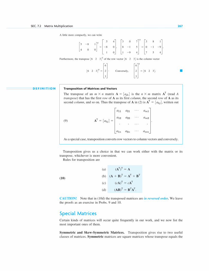
A little more compactly, we can write
Furthermore, the transpose of the row vector is the column vector
D E F I N I T I O N Transposition of Matrices and Vectors
The transpose of an matrix is the matrix (read Atranspose) that has the first row of A as its first column, the second row of A as itssecond column, and so on. Thus the transpose of A in (2) is written out
(9)
As a special case, transposition converts row vectors to column vectors and conversely.
Transposition gives us a choice in that we can work either with the matrix or itstranspose, whichever is more convenient.
Rules for transposition are
(a)
(10)(b)
(c)
(d)
CAUTION! Note that in (10d) the transposed matrices are in reversed order. We leavethe proofs as an exercise in Probs. 9 and 10.
Special MatricesCertain kinds of matrices will occur quite frequently in our work, and we now list themost important ones of them.
Symmetric and Skew-Symmetric Matrices. Transposition gives rise to two usefulclasses of matrices. Symmetric matrices are square matrices whose transpose equals the
(AB)T � BTAT.
(cA)T � cAT
(A � B)T � AT � BT
(AT)T � A
AT � 3akj4 � Ea11
a12
#
a1n
a21
a22
#
a2n
Á
Á
Á
Á
am1
am2
#
amn
U .
AT � 3akj4,
ATn � mA � 3ajk4m � n
�36 2 34T � D623
T # Conversely, D623
TT
� 36 2 34.
36 2 3436 2 34T
c54
�8
0
1
0d T � D 5
�8
1
4
0
0
T , D381
0
�1
�9
7
5
4
T T
� D307
8
�1
5
1
�9
4
T ,
SEC. 7.2 Matrix Multiplication 267

matrix itself. Skew-symmetric matrices are square matrices whose transpose equalsminus the matrix. Both cases are defined in (11) and illustrated by Example 8.
(11) (thus (thus hence
Symmetric Matrix Skew-Symmetric Matrix
E X A M P L E 8 Symmetric and Skew-Symmetric Matrices
is symmetric, and is skew-symmetric.
For instance, if a company has three building supply centers then A could show costs, say, forhandling 1000 bags of cement at center , and the cost of shipping 1000 bags from to . Clearly,
if we assume shipping in the opposite direction will cost the same.Symmetric matrices have several general properties which make them important. This will be seen as we
proceed.
Triangular Matrices. Upper triangular matrices are square matrices that can have nonzeroentries only on and above the main diagonal, whereas any entry below the diagonal must bezero. Similarly, lower triangular matrices can have nonzero entries only on and below themain diagonal. Any entry on the main diagonal of a triangular matrix may be zero or not.
E X A M P L E 9 Upper and Lower Triangular Matrices
Upper triangular Lower triangular
Diagonal Matrices. These are square matrices that can have nonzero entries only onthe main diagonal. Any entry above or below the main diagonal must be zero.
If all the diagonal entries of a diagonal matrix S are equal, say, c, we call S a scalarmatrix because multiplication of any square matrix A of the same size by S has the sameeffect as the multiplication by a scalar, that is,
(12)
In particular, a scalar matrix, whose entries on the main diagonal are all 1, is called a unitmatrix (or identity matrix) and is denoted by or simply by I. For I, formula (12) becomes
(13)
E X A M P L E 1 0 Diagonal Matrix D. Scalar Matrix S. Unit Matrix I
�D � D200
0
�3
0
0
0
0
T , S � Dc00
0
c
0
0
0
c
T , I � D100
0
1
0
0
0
1
TAI � IA � A.
In
AS � SA � cA.
�E391
1
0
�3
0
9
0
0
2
3
0
0
0
6
U .c10
3
2d , D10
0
4
3
0
2
2
6
T , D287
0
�1
6
0
0
8
T ,
�
ajk � akj
CkCjajk ( j � k)Cj
ajjC1, C2, C3,
B � D 0
�1
3
1
0
2
�3
�2
0
TA � D 20
120
200
120
10
150
200
150
30
T
ajj � 0).akj � �ajk,akj � ajk), AT � �AAT � A
268 CHAP. 7 Linear Algebra: Matrices, Vectors, Determinants. Linear Systems

Some Applications of Matrix MultiplicationE X A M P L E 1 1 Computer Production. Matrix Times Matrix
Supercomp Ltd produces two computer models PC1086 and PC1186. The matrix A shows the cost per computer(in thousands of dollars) and B the production figures for the year 2010 (in multiples of 10,000 units.) Find amatrix C that shows the shareholders the cost per quarter (in millions of dollars) for raw material, labor, andmiscellaneous.
QuarterPC1086 PC1186 1 2 3 4
Solution.
Quarter1 2 3 4
Since cost is given in multiples of and production in multiples of 10,000 units, the entries of C aremultiples of millions; thus means million, etc.
E X A M P L E 1 2 Weight Watching. Matrix Times Vector
Suppose that in a weight-watching program, a person of 185 lb burns 350 cal/hr in walking (3 mph), 500 inbicycling (13 mph), and 950 in jogging (5.5 mph). Bill, weighing 185 lb, plans to exercise according to thematrix shown. Verify the calculations
W B J
E X A M P L E 1 3 Markov Process. Powers of a Matrix. Stochastic Matrix
Suppose that the 2004 state of land use in a city of of built-up area is
C: Commercially Used 25% I: Industrially Used 20% R: Residentially Used 55%.
Find the states in 2009, 2014, and 2019, assuming that the transition probabilities for 5-year intervals are givenby the matrix A and remain practically the same over the time considered.
From C From I From R
A � D0.7
0.2
0.1
0.1
0.9
0
0
0.2
0.8
T
To C
To I
To R
60 mi2
�
MON
WED
FRI
SAT
E1.0
1.0
1.5
2.0
0
1.0
0
1.5
0.5
0.5
0.5
1.0
U D350
500
950
T � E 825
1325
1000
2400
U MON
WED
FRI
SAT
1W � Walking, B � Bicycling, J � Jogging2.
�$132c11 � 13.2$10$1000
C � AB � D13.2
3.3
5.1
12.8
3.2
5.2
13.6
3.4
5.4
15.6
3.9
6.3
T Raw Components
Labor
Miscellaneous
B � c36
8
2
6
4
9
3d PC1086
PC1186A � D1.2
0.3
0.5
1.6
0.4
0.6
T Raw Components
Labor
Miscellaneous
SEC. 7.2 Matrix Multiplication 269

A is a stochastic matrix, that is, a square matrix with all entries nonnegative and all column sums equal to 1.Our example concerns a Markov process,1 that is, a process for which the probability of entering a certain statedepends only on the last state occupied (and the matrix A), not on any earlier state.
Solution. From the matrix A and the 2004 state we can compute the 2009 state,
To explain: The 2009 figure for C equals times the probability 0.7 that C goes into C, plus times theprobability 0.1 that I goes into C, plus times the probability 0 that R goes into C. Together,
Also
Similarly, the new R is . We see that the 2009 state vector is the column vector
where the column vector is the given 2004 state vector. Note that the sum of the entries ofy is . Similarly, you may verify that for 2014 and 2019 we get the state vectors
Answer. In 2009 the commercial area will be the industrial and theresidential . For 2014 the corresponding figures are and . For 2019they are and . (In Sec. 8.2 we shall see what happens in the limit, assuming thatthose probabilities remain the same. In the meantime, can you experiment or guess?) �
33.025%16.315%, 50.660%,39.15%17.05%, 43.80%,46.5% (27.9 mi2)
34% (20.4 mi2),19.5% (11.7 mi2),
u � Az � A2y � A3x � 316.315 50.660 33.0254T.
z � Ay � A(Ax) � A2x � 317.05 43.80 39.154T
100 3%4x � 325 20 554T
y � 319.5 34.0 46.54T � Ax � A 325 20 554T
46.5%
25 # 0.2 � 20 # 0.9 � 55 # 0.2 � 34 3%4.25 # 0.7 � 20 # 0.1 � 55 # 0 � 19.5 3%4.
55%20%25%
C
I
R
D0.7 # 25 � 0.1 # 20 � 0 # 55
0.2 # 25 � 0.9 # 20 � 0.2 # 55
0.1 # 25 � 0 # 20 � 0.8 # 55
T � D0.7
0.2
0.1
0.1
0.9
0
0
0.2
0.8
T D25
20
55
T � D19.5
34.0
46.5
T .
270 CHAP. 7 Linear Algebra: Matrices, Vectors, Determinants. Linear Systems
1–10 GENERAL QUESTIONS1. Multiplication. Why is multiplication of matrices
restricted by conditions on the factors?
2. Square matrix. What form does a matrix haveif it is symmetric as well as skew-symmetric?
3. Product of vectors. Can every matrix berepresented by two vectors as in Example 3?
4. Skew-symmetric matrix. How many different entriescan a skew-symmetric matrix have? An skew-symmetric matrix?
5. Same questions as in Prob. 4 for symmetric matrices.
6. Triangular matrix. If are upper triangular andare lower triangular, which of the following are
triangular?
7. Idempotent matrix, defined by Can you findfour idempotent matrices?2 � 2
A2 � A.
L1 � L2
U1L1,U1 � U2, U1U2, U12, U1 � L1,
L1, L2
U1, U2
n � n4 � 4
3 � 3
3 � 3
P R O B L E M S E T 7 . 2
8. Nilpotent matrix, defined by for some m.Can you find three nilpotent matrices?
9. Transposition. Can you prove (10a)–(10c) for matrices? For matrices?
10. Transposition. (a) Illustrate (10d) by simple examples.(b) Prove (10d).
11–20 MULTIPLICATION, ADDITION, ANDTRANSPOSITION OF MATRICES ANDVECTORS
Let
C � D 0
3
�2
1
2
0
T , a � 31 �2 04, b � D 3
1
�1
T .
A � D 4
�2
1
�2
1
2
3
6
2
T , B � D 1
�3
0
�3
1
0
0
0
�2
T
m � n3 � 3
2 � 2Bm � 0
1ANDREI ANDREJEVITCH MARKOV (1856–1922), Russian mathematician, known for his work inprobability theory.

Showing all intermediate results, calculate the followingexpressions or give reasons why they are undefined:
11.
12.
13.
14.
15.
16.
17.
18.
19.
20.
21. General rules. Prove (2) for matrices and a general scalar.
22. Product. Write AB in Prob. 11 in terms of row andcolumn vectors.
23. Product. Calculate AB in Prob. 11 columnwise. SeeExample 1.
24. Commutativity. Find all matrices that commute with , where
25. TEAM PROJECT. Symmetric and Skew-SymmetricMatrices. These matrices occur quite frequently inapplications, so it is worthwhile to study some of theirmost important properties.
(a) Verify the claims in (11) that for asymmetric matrix, and for a skew-symmetric matrix. Give examples.
(b) Show that for every square matrix C the matrixis symmetric and is skew-symmetric.
Write C in the form , where S is symmetricand T is skew-symmetric and find S and T in termsof C. Represent A and B in Probs. 11–20 in this form.
(c) A linear combination of matrices A, B, C, , Mof the same size is an expression of the form
(14)
where a, , m are any scalars. Show that if thesematrices are square and symmetric, so is (14); similarly,if they are skew-symmetric, so is (14).
(d) Show that AB with symmetric A and B is symmetricif and only if A and B commute, that is,
(e) Under what condition is the product of skew-symmetric matrices skew-symmetric?
26–30 FURTHER APPLICATIONS26. Production. In a production process, let N mean “no
trouble” and T “trouble.” Let the transition probabilitiesfrom one day to the next be 0.8 for , hence 0.2for , and 0.5 for , hence 0.5 for T : T.T : NN : T
N : N
AB � BA.
Á
aA � bB � cC � Á � mM,
Á
C � S � TC � CTC � CT
akj � �ajk
akj � ajk
bjk � j � k.B � 3bjk4A � 3ajk42 � 2
B � 3bjk4, C � 3cjk4,A � 3ajk4,2 � 2
bTAb, aBaT, aCCT, CTba
Ab � Bb(A � B)b,1.5a � 3.0b, 1.5aT � 3.0b,
ab, ba, aA, Bb
ABC, ABa, ABb, CaT
BC, BCT, Bb, bTB
bTATAa, AaT, (Ab)T,
(3A � 2B)TaT3AT � 2BT,3A � 2B, (3A � 2B)T,
CCT, BC, CB, CTB
AAT, A2, BBT, B2
AB, ABT, BA, BTA
SEC. 7.2 Matrix Multiplication 271
If today there is no trouble, what is the probability ofN two days after today? Three days after today?
27. CAS Experiment. Markov Process. Write a programfor a Markov process. Use it to calculate further stepsin Example 13 of the text. Experiment with otherstochastic matrices, also using different startingvalues.
28. Concert subscription. In a community of 100,000adults, subscribers to a concert series tend to renew theirsubscription with probability and persons presentlynot subscribing will subscribe for the next season withprobability . If the present number of subscribersis 1200, can one predict an increase, decrease, or nochange over each of the next three seasons?
29. Profit vector. Two factory outlets and in NewYork and Los Angeles sell sofas (S), chairs (C), andtables (T) with a profit of , and , respectively.Let the sales in a certain week be given by the matrix
S C T
Introduce a “profit vector” p such that the componentsof give the total profits of and .
30. TEAM PROJECT. Special Linear Transformations.Rotations have various applications. We show in thisproject how they can be handled by matrices.
(a) Rotation in the plane. Show that the lineartransformation with
is a counterclockwise rotation of the Cartesian -coordinate system in the plane about the origin, where
is the angle of rotation.
(b) Rotation through n�. Show that in (a)
Is this plausible? Explain this in words.
(c) Addition formulas for cosine and sine. Bygeometry we should have
Derive from this the addition formulas (6) in App. A3.1.
� c cos (a � b)
sin (a � b)
�sin (a � b)
cos (a � b)d .
c cos a
sin a
�sin a
cos ad c cos b
sin b
�sin b
cos bd
An � c cos nu
sin nu
�sin nu
cos nud .
u
x1x2
A � c cos u
sin u
�sin u
cos ud , x � c x1
x2
d , y � c y1
y2
dy � Ax
F2F1v � Ap
A � c400
100
60
120
240
500d F1
F2
$30$35, $62
F2F1
0.2%
90%
3 � 3
7.3 Linear Systems of Equations. Gauss Elimination
We now come to one of the most important use of matrices, that is, using matrices tosolve systems of linear equations. We showed informally, in Example 1 of Sec. 7.1, howto represent the information contained in a system of linear equations by a matrix, calledthe augmented matrix. This matrix will then be used in solving the linear system ofequations. Our approach to solving linear systems is called the Gauss elimination method.Since this method is so fundamental to linear algebra, the student should be alert.
A shorter term for systems of linear equations is just linear systems. Linear systemsmodel many applications in engineering, economics, statistics, and many other areas.Electrical networks, traffic flow, and commodity markets may serve as specific examplesof applications.
Linear System, Coefficient Matrix, Augmented MatrixA linear system of m equations in n unknowns is a set of equations ofthe form
(1)
The system is called linear because each variable appears in the first power only, justas in the equation of a straight line. are given numbers, called the coefficientsof the system. on the right are also given numbers. If all the are zero, then(1) is called a homogeneous system. If at least one is not zero, then (1) is called anonhomogeneous system.
bj
bjb1, Á , bm
a11, Á , amn
x j
a11x1 � Á � a1nxn � b1
a21x1 � Á � a2nxn � b2
. . . . . . . . . . . . . . . . . . . . . . .
am1x1 � Á � amnxn � bm.
x1, Á , xn
272 CHAP. 7 Linear Algebra: Matrices, Vectors, Determinants. Linear Systems
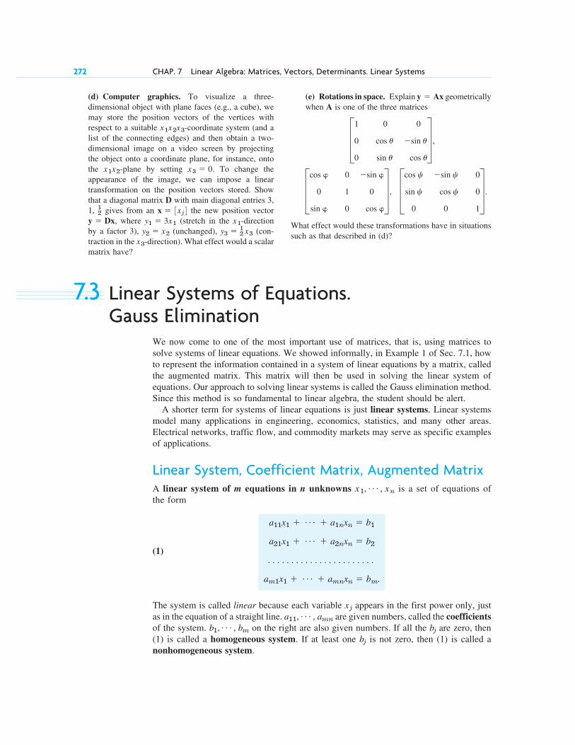
(d) Computer graphics. To visualize a three-dimensional object with plane faces (e.g., a cube), wemay store the position vectors of the vertices withrespect to a suitable -coordinate system (and alist of the connecting edges) and then obtain a two-dimensional image on a video screen by projectingthe object onto a coordinate plane, for instance, ontothe -plane by setting . To change theappearance of the image, we can impose a lineartransformation on the position vectors stored. Showthat a diagonal matrix D with main diagonal entries 3,1, gives from an the new position vector
, where (stretch in the -directionby a factor 3), (unchanged), (con-traction in the -direction). What effect would a scalarmatrix have?
x3
y3 � 12 x3y2 � x2
x1y1 � 3x1y � Dxx � 3x j4
12
x3 � 0x1x2
x1x2x3
(e) Rotations in space. Explain geometricallywhen A is one of the three matrices
What effect would these transformations have in situationssuch as that described in (d)?
Dcos �
0
sin �
0
1
0
�sin �
0
cos �
T , Dcos c
sin c
0
�sin c
cos c
0
0
0
1
T .
D100
0
cos u
sin u
0
�sin u
cos u
T ,
y � Ax

A solution of (1) is a set of numbers that satisfies all the m equations.A solution vector of (1) is a vector x whose components form a solution of (1). If thesystem (1) is homogeneous, it always has at least the trivial solution
Matrix Form of the Linear System (1). From the definition of matrix multiplicationwe see that the m equations of (1) may be written as a single vector equation
(2)
where the coefficient matrix is the matrix
and and
are column vectors. We assume that the coefficients are not all zero, so that A isnot a zero matrix. Note that x has n components, whereas b has m components. Thematrix
is called the augmented matrix of the system (1). The dashed vertical line could beomitted, as we shall do later. It is merely a reminder that the last column of did notcome from matrix A but came from vector b. Thus, we augmented the matrix A.
Note that the augmented matrix determines the system (1) completely because itcontains all the given numbers appearing in (1).
E X A M P L E 1 Geometric Interpretation. Existence and Uniqueness of Solutions
If we have two equations in two unknowns
If we interpret as coordinates in the -plane, then each of the two equations represents a straight line,and is a solution if and only if the point P with coordinates lies on both lines. Hence there arethree possible cases (see Fig. 158 on next page):
(a) Precisely one solution if the lines intersect
(b) Infinitely many solutions if the lines coincide
(c) No solution if the lines are parallel
x1, x2(x1, x2)x1x2x1, x2
a11x1 � a12x2 � b1
a21x1 � a22x2 � b2.
x1, x2m � n � 2,
A~
A~
A~ � Ea11Á a1n b1
# Á # #
# Á # #
am1Á amn bm
Uajk
b � Db1
.
.
.bm
Tx � Gx1
#
#
#
xn
WA � Ea11
a21
#
am1
a12
a22
#
am2
Á
Á
Á
Á
a1n
a2n
#
amn
U ,
m � nA � 3ajk4
Ax � b
x1 � 0, Á , xn � 0.
x1, Á , xn
SEC. 7.3 Linear Systems of Equations. Gauss Elimination 273
|
|
|
|
|
|

For instance,
274 CHAP. 7 Linear Algebra: Matrices, Vectors, Determinants. Linear Systems
Unique solution
Infinitely many solutions
No solution
Fig. 158. Threeequations in
three unknownsinterpreted asplanes in space
1
x2 x2 x2
1 1 x1x1x1
x1 + x2 = 1
2x1 – x2 = 0
Case (a)
x1 + x2 = 1
2x1 + 2x2 = 2
Case (b)
x1 + x2 = 1
x1 + x2 = 0
Case (c)
13
23
P
If the system is homogenous, Case (c) cannot happen, because then those two straight lines pass through theorigin, whose coordinates constitute the trivial solution. Similarly, our present discussion can be extendedfrom two equations in two unknowns to three equations in three unknowns. We give the geometric interpretationof three possible cases concerning solutions in Fig. 158. Instead of straight lines we have planes and the solutiondepends on the positioning of these planes in space relative to each other. The student may wish to come upwith some specific examples.
Our simple example illustrated that a system (1) may have no solution. This leads to suchquestions as: Does a given system (1) have a solution? Under what conditions does it haveprecisely one solution? If it has more than one solution, how can we characterize the setof all solutions? We shall consider such questions in Sec. 7.5.
First, however, let us discuss an important systematic method for solving linear systems.
Gauss Elimination and Back SubstitutionThe Gauss elimination method can be motivated as follows. Consider a linear system thatis in triangular form (in full, upper triangular form) such as
(Triangular means that all the nonzero entries of the corresponding coefficient matrix lieabove the diagonal and form an upside-down triangle.) Then we can solve the systemby back substitution, that is, we solve the last equation for the variable, and then work backward, substituting into the first equation and solving it for , obtaining This gives us the idea of first reducinga general system to triangular form. For instance, let the given system be
Its augmented matrix is
We leave the first equation as it is. We eliminate from the second equation, to get atriangular system. For this we add twice the first equation to the second, and we do the same
x1
c 2
�4
5
3
2
�30d .2x1 � 5x2 � 2
�4x1 � 3x2 � �30.
x1 � 12 (2 � 5x2) � 1
2 (2 � 5 # (�2)) � 6.x1x2 � �2
x2 � �26>13 � �2,90°
13x2 � �26
2x1 � 5x2 � 2
�
(0, 0)
operation on the rows of the augmented matrix. This gives that is,
where means “Add twice Row 1 to Row 2” in the original matrix. Thisis the Gauss elimination (for 2 equations in 2 unknowns) giving the triangular form, fromwhich back substitution now yields and , as before.
Since a linear system is completely determined by its augmented matrix, Gausselimination can be done by merely considering the matrices, as we have just indicated.We do this again in the next example, emphasizing the matrices by writing them first andthe equations behind them, just as a help in order not to lose track.
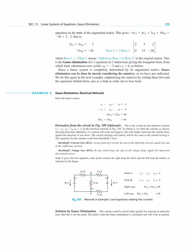
E X A M P L E 2 Gauss Elimination. Electrical Network
Solve the linear system
Derivation from the circuit in Fig. 159 (Optional ). This is the system for the unknown currentsin the electrical network in Fig. 159. To obtain it, we label the currents as shown,
choosing directions arbitrarily; if a current will come out negative, this will simply mean that the current flowsagainst the direction of our arrow. The current entering each battery will be the same as the current leaving it.The equations for the currents result from Kirchhoff’s laws:
Kirchhoff’s Current Law (KCL). At any point of a circuit, the sum of the inflowing currents equals the sumof the outflowing currents.
Kirchhoff’s Voltage Law (KVL). In any closed loop, the sum of all voltage drops equals the impressedelectromotive force.
Node P gives the first equation, node Q the second, the right loop the third, and the left loop the fourth, asindicated in the figure.
x2 � i2, x3 � i3x1 � i1,
x1 � x2 � x3 � 0
�x1 � x2 � x3 � 0
10x2 � 25x3 � 90
20x1 � 10x2 � 80.
x1 � 6x2 � �2
Row 2 � 2 Row 1
c20
5
13
2
�26d
Row 2 � 2 Row 1
2x1 � 5x2 � 2
13x2 � �26
�30 � 2 # 2,�4x1 � 4x1 � 3x2 � 10x2 �
SEC. 7.3 Linear Systems of Equations. Gauss Elimination 275
20 Ω 10 Ω
15 Ω
10 Ω 90 V80 V
i1 i3
i2
Node P: i1 – i
2 + i
3 = 0
Node Q:
Q
P
– i1 + i
2 – i
3 = 0
Right loop: 10i2 + 25 i
3 = 90
Left loop: 20i1 + 10 i
2 = 80
Fig. 159. Network in Example 2 and equations relating the currents
Solution by Gauss Elimination. This system could be solved rather quickly by noticing its particularform. But this is not the point. The point is that the Gauss elimination is systematic and will work in general,

ö
ö ö
ö
ö
ö
ö
ö
276 CHAP. 7 Linear Algebra: Matrices, Vectors, Determinants. Linear Systems
Pivot 1
Eliminate
Pivot 1
Eliminate
also for large systems. We apply it to our system and then do back substitution. As indicated, let us write theaugmented matrix of the system first and then the system itself:
Augmented Matrix Equations
Step 1. Elimination of Call the first row of A the pivot row and the first equation the pivot equation. Call the coefficient 1 of its
-term the pivot in this step. Use this equation to eliminate (get rid of in the other equations. For this, do:
Add 1 times the pivot equation to the second equation.
Add times the pivot equation to the fourth equation.
This corresponds to row operations on the augmented matrix as indicated in BLUE behind the new matrix in(3). So the operations are performed on the preceding matrix. The result is
(3)
Step 2. Elimination of The first equation remains as it is. We want the new second equation to serve as the next pivot equation. Butsince it has no x2-term (in fact, it is , we must first change the order of the equations and the correspondingrows of the new matrix. We put at the end and move the third equation and the fourth equation one placeup. This is called partial pivoting (as opposed to the rarely used total pivoting, in which the order of theunknowns is also changed). It gives
To eliminate , do:
Add times the pivot equation to the third equation.The result is
(4)
Back Substitution. Determination of (in this order)Working backward from the last to the first equation of this “triangular” system (4), we can now readily find
, then , and then :
where A stands for “amperes.” This is the answer to our problem. The solution is unique. �
x3 � i3 � 2 3A4
x2 � 110 (90 � 25x3) � i2 � 4 3A4
x1 � x2 � x3 � i1 � 2 3A4
� 95x3 � �190
10x2 � 25x3 � 90
x1 � x2 � x3 � 0
x1x2x3
x3, x2, x1
x1 � x2 � x3 � 0
10x2 � 25x3 � 90
� 95x3 � �190
0 � 0.
Row 3 � 3 Row 2E1 �1 1 0
0 10 25 90
0 0 �95 �190
0 0 0 0
U�3
x2
x1 � x2 � x3 � 0
10x2 � 25x3 � 90
30x2 � 20x3 � 80
0 � 0.
Pivot 10
Eliminate 30x2
E1 �1 1 0
0 10 25 90
0 30 �20 80
0 0 0 0
UPivot 10
Eliminate 30
0 � 00 � 0)
x2
x1 � x2 � x3 � 0
0 � 0
10x2 � 25x3 � 90
30x2 � 20x3 � 80.
Row 2 � Row 1
Row 4 � 20 Row 1
E1 �1 1 0
0 0 0 0
0 10 25 90
0 30 �20 80
U�20
x1)x1x1
x1
x1 � x2 � x3 � 0
�x1 � x2 � x3 � 0
10x2 � 25x3 � 90
20x1 � 10x2 � 80.
E
1 �1 1 0
�1 1 �1 0
0 10 25 90
20 10 0 80
UA~
|||||||||
|||||||
|||||||
|||||||

Elementary Row Operations. Row-Equivalent SystemsExample 2 illustrates the operations of the Gauss elimination. These are the first two ofthree operations, which are called
Elementary Row Operations for Matrices:
Interchange of two rows
Addition of a constant multiple of one row to another row
Multiplication of a row by a nonzero constant c
CAUTION! These operations are for rows, not for columns! They correspond to thefollowing
Elementary Operations for Equations:
Interchange of two equations
Addition of a constant multiple of one equation to another equation
Multiplication of an equation by a nonzero constant c
Clearly, the interchange of two equations does not alter the solution set. Neither does theiraddition because we can undo it by a corresponding subtraction. Similarly for theirmultiplication, which we can undo by multiplying the new equation by (since producing the original equation.
We now call a linear system row-equivalent to a linear system if can beobtained from by (finitely many!) row operations. This justifies Gauss elimination andestablishes the following result.
T H E O R E M 1 Row-Equivalent Systems
Row-equivalent linear systems have the same set of solutions.
Because of this theorem, systems having the same solution sets are often calledequivalent systems. But note well that we are dealing with row operations. No columnoperations on the augmented matrix are permitted in this context because they wouldgenerally alter the solution set.
A linear system (1) is called overdetermined if it has more equations than unknowns,as in Example 2, determined if , as in Example 1, and underdetermined if it hasfewer equations than unknowns.
Furthermore, a system (1) is called consistent if it has at least one solution (thus, onesolution or infinitely many solutions), but inconsistent if it has no solutions at all, as
in Example 1, Case (c).
Gauss Elimination: The Three Possible Cases of SystemsWe have seen, in Example 2, that Gauss elimination can solve linear systems that have aunique solution. This leaves us to apply Gauss elimination to a system with infinitelymany solutions (in Example 3) and one with no solution (in Example 4).
x1 � x2 � 1, x1 � x2 � 0
m � n
S2
S1S2S1
c � 0),1>c
SEC. 7.3 Linear Systems of Equations. Gauss Elimination 277
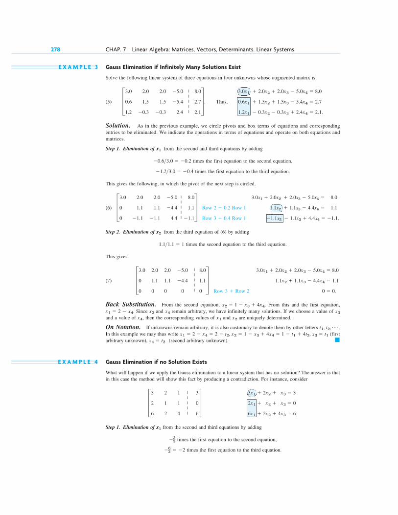
E X A M P L E 3 Gauss Elimination if Infinitely Many Solutions Exist
Solve the following linear system of three equations in four unknowns whose augmented matrix is
(5) Thus,
Solution. As in the previous example, we circle pivots and box terms of equations and correspondingentries to be eliminated. We indicate the operations in terms of equations and operate on both equations andmatrices.
Step 1. Elimination of from the second and third equations by adding
times the first equation to the second equation,
times the first equation to the third equation.
This gives the following, in which the pivot of the next step is circled.
(6)
Step 2. Elimination of from the third equation of (6) by adding
times the second equation to the third equation.
This gives
(7)
Back Substitution. From the second equation, . From this and the first equation,. Since and remain arbitrary, we have infinitely many solutions. If we choose a value of
and a value of , then the corresponding values of and are uniquely determined.
On Notation. If unknowns remain arbitrary, it is also customary to denote them by other letters In this example we may thus write (firstarbitrary unknown), (second arbitrary unknown).
E X A M P L E 4 Gauss Elimination if no Solution Exists
What will happen if we apply the Gauss elimination to a linear system that has no solution? The answer is thatin this case the method will show this fact by producing a contradiction. For instance, consider
Step 1. Elimination of from the second and third equations by adding
times the first equation to the second equation,
times the first equation to the third equation.�63 � �2
�23
x1
3x1 � 2x2 � x3 � 3
2x1 � x2 � x3 � 0
6x1 � 2x2 � 4x3 � 6.
D3 2 1 3
2 1 1 0
6 2 4 6
T
�x4 � t2
x1 � 2 � x4 � 2 � t2, x2 � 1 � x3 � 4x4 � 1 � t1 � 4t2, x3 � t1
t1, t2, Á .
x2x1x4
x3x4x3x1 � 2 � x4
x2 � 1 � x3 � 4x4
3.0x1 � 2.0x2 � 2.0x3 � 5.0x4 � 8.0
1.1x2 � 1.1x3 � 4.4x4 � 1.1
0 � 0.Row 3 � Row 2
D3.0 2.0 2.0 �5.0 8.0
0 1.1 1.1 �4.4 1.1
0 0 0 0 0
T1.1>1.1 � 1
x2
3.0x1 � 2.0x2 � 2.0x3 � 5.0x4 � 8.0
1.1x2 � 1.1x3 � 4.4x4 � 1.1
�1.1x2 � 1.1x3 � 4.4x4 � �1.1.
Row 2 � 0.2 Row 1
Row 3 � 0.4 Row 1
D3.0 2.0 2.0 �5.0 8.0
0 1.1 1.1 �4.4 1.1
0 �1.1 �1.1 4.4 �1.1
T�1.2>3.0 � �0.4
�0.6>3.0 � �0.2
x1
3.0x1 � 2.0x2 � 2.0x3 � 5.0x4 � 8.0
0.6x1 � 1.5x2 � 1.5x3 � 5.4x4 � 2.7
1.2x1 � 0.3x2 � 0.3x3 � 2.4x4 � 2.1.
D3.0 2.0 2.0 �5.0 8.0
0.6 1.5 1.5 �5.4 2.7
1.2 �0.3 �0.3 2.4 2.1
T .
278 CHAP. 7 Linear Algebra: Matrices, Vectors, Determinants. Linear Systems
|||||
|||||
|||||
|||||
This gives
Step 2. Elimination of from the third equation gives
The false statement shows that the system has no solution.
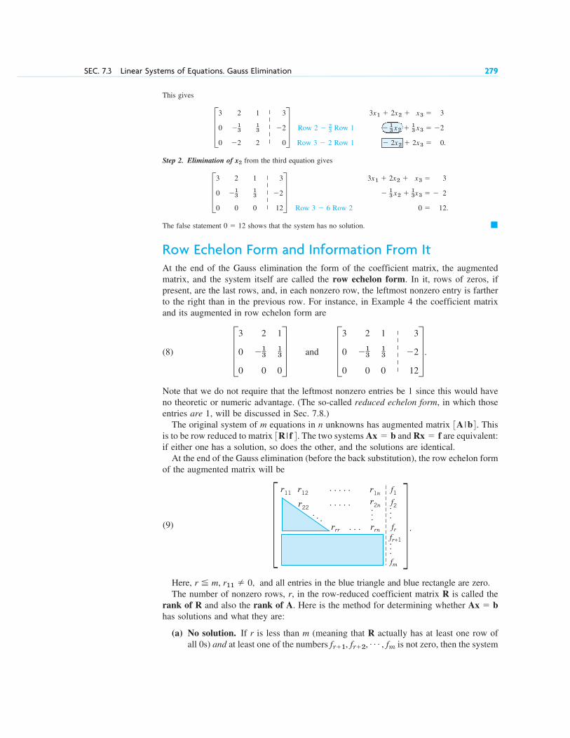
Row Echelon Form and Information From ItAt the end of the Gauss elimination the form of the coefficient matrix, the augmentedmatrix, and the system itself are called the row echelon form. In it, rows of zeros, ifpresent, are the last rows, and, in each nonzero row, the leftmost nonzero entry is fartherto the right than in the previous row. For instance, in Example 4 the coefficient matrixand its augmented in row echelon form are
(8) and
Note that we do not require that the leftmost nonzero entries be 1 since this would haveno theoretic or numeric advantage. (The so-called reduced echelon form, in which thoseentries are 1, will be discussed in Sec. 7.8.)
The original system of m equations in n unknowns has augmented matrix . Thisis to be row reduced to matrix . The two systems and are equivalent:if either one has a solution, so does the other, and the solutions are identical.
At the end of the Gauss elimination (before the back substitution), the row echelon formof the augmented matrix will be
Rx � fAx � b3R | f 43A | b4
D3 2 1 3
0 �13
13 �2
0 0 0 12
T .D3 2 1
0 �13
13
0 0 0
T
�0 � 12
3x1 � 2x2 � x3 � 3
� 13 x2 � 1
3x3 � � 2
0 � 12.Row 3 � 6 Row 2
D3 2 1 3
0 �13
13 �2
0 0 0 12
Tx2
3x1 � 2x2 � x3 � 3
� 13 x2 � 1
3 x3 � �2
� 2x2 � 2x3 � 0.
Row 2 � 2_3 Row 1
Row 3 � 2 Row 1
D3 2 1 3
0 �13
13 �2
0 �2 2 0
TSEC. 7.3 Linear Systems of Equations. Gauss Elimination 279
|||||
|||||
||||||
...
......
. . .
. . .. . . . .
. . . . .
rrr rrn fr
fm
f1r2nr22
r12 r1nr11
f2
fr+1
Here, and all entries in the blue triangle and blue rectangle are zero.The number of nonzero rows, r, in the row-reduced coefficient matrix R is called the
rank of R and also the rank of A. Here is the method for determining whether has solutions and what they are:
(a) No solution. If r is less than m (meaning that R actually has at least one row ofall 0s) and at least one of the numbers is not zero, then the systemfr�1, fr�2, Á , fm
Ax � b
r � m, r11 � 0,
(9) X.
X

280 CHAP. 7 Linear Algebra: Matrices, Vectors, Determinants. Linear Systems
1–14 GAUSS ELIMINATIONSolve the linear system given explicitly or by its augmentedmatrix. Show details.
1.
�3x � 8y � 10
4x � 6y � �11
12.
13.
14.
15. Equivalence relation. By definition, an equivalencerelation on a set is a relation satisfying three conditions:(named as indicated)
(i) Each element A of the set is equivalent to itself(Reflexivity).
(ii) If A is equivalent to B, then B is equivalent to A(Symmetry).
(iii) If A is equivalent to B and B is equivalent to C,then A is equivalent to C (Transitivity).
Show that row equivalence of matrices satisfies thesethree conditions. Hint. Show that for each of the threeelementary row operations these conditions hold.
E2 3 1 �11 1
5 �2 5 �4 5
1 �1 3 �3 3
3 4 �7 2 �7
U 8w � 34x � 16y � 10z � 4
w � x � y � 6
�3w � 17x � y � 2z � 2
10x � 4y � 2z � �4
D 2 �2 4 0 0
�3 3 �6 5 15
1 �1 2 0 0
TP R O B L E M S E T 7 . 3
is inconsistent: No solution is possible. Therefore the system isinconsistent as well. See Example 4, where and
If the system is consistent (either or and all the numbers are zero), then there are solutions.
(b) Unique solution. If the system is consistent and , there is exactly onesolution, which can be found by back substitution. See Example 2, where and
(c) Infinitely many solutions. To obtain any of these solutions, choose values ofarbitrarily. Then solve the rth equation for (in terms of those
arbitrary values), then the st equation for , and so on up the line. SeeExample 3.
Orientation. Gauss elimination is reasonable in computing time and storage demand.We shall consider those aspects in Sec. 20.1 in the chapter on numeric linear algebra.Section 7.4 develops fundamental concepts of linear algebra such as linear independenceand rank of a matrix. These in turn will be used in Sec. 7.5 to fully characterize thebehavior of linear systems in terms of existence and uniqueness of solutions.
xr�1(r � 1)xrx r�1, Á , xn
m � 4.r � n � 3
r � n
fr�1, fr�2, Á , fmr mr � m,
fr�1 � f3 � 12.r � 2 m � 3Ax � bRx � f
2. c3.0 �0.5 0.6
1.5 4.5 6.0d
3.
�2x � 4y � 6z � 40
8y � 6z � �6
x � y � z � 9 4. D 4 1 0 4
5 �3 1 2
�9 2 �1 5
T5. D 13 12 �6
�4 7 �73
11 �13 157
T 6. D 4 �8 3 16
�1 2 �5 �21
3 �6 1 7
T7. D 2 4 1 0
�1 1 �2 0
4 0 6 0
T 8.
3x � 2y � 5
2x � z � 2
4y � 3z � 8
9.
3x � 4y � 5z � 13
�2y � 2z � �8 10. c 5 �7 3 17
�15 21 �9 50d
11. D0 5 5 �10 0
2 �3 �3 6 2
4 1 1 �2 4
T
16. CAS PROJECT. Gauss Elimination and BackSubstitution. Write a program for Gauss eliminationand back substitution (a) that does not include pivotingand (b) that does include pivoting. Apply the programsto Probs. 11–14 and to some larger systems of yourchoice.
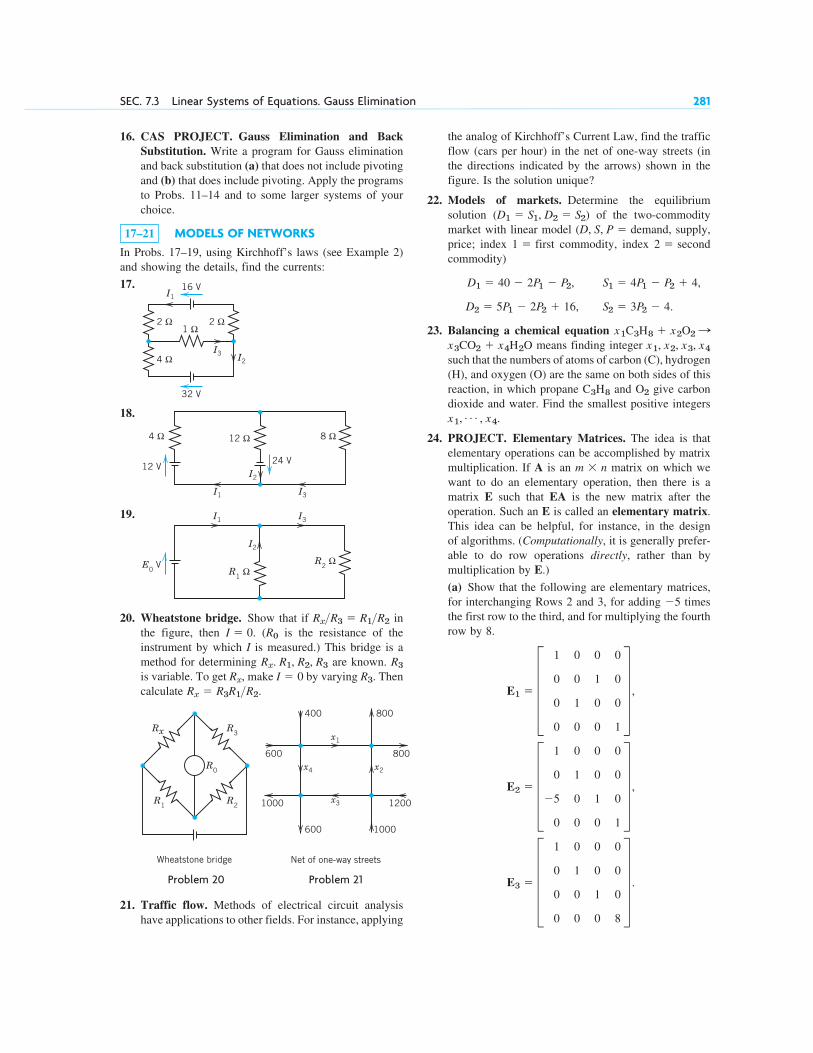
17–21 MODELS OF NETWORKSIn Probs. 17–19, using Kirchhoff’s laws (see Example 2)and showing the details, find the currents:
17.
18.
19.
20. Wheatstone bridge. Show that if inthe figure, then . ( is the resistance of theinstrument by which I is measured.) This bridge is amethod for determining are known. is variable. To get , make by varying . Thencalculate .Rx � R3R1>R2
R3I � 0Rx
R3Rx. R1, R2, R3
R0I � 0Rx>R3 � R1>R2
R1 Ω
R2 Ω
I2
I1
E0 V
I3
12 Ω4 Ω
24 V
8 Ω
I2
I1
12 V
I3
1 Ω2 Ω 2 Ω
4 Ω
32 V
I3
I1
I2
16 V
SEC. 7.3 Linear Systems of Equations. Gauss Elimination 281
the analog of Kirchhoff’s Current Law, find the trafficflow (cars per hour) in the net of one-way streets (inthe directions indicated by the arrows) shown in thefigure. Is the solution unique?
22. Models of markets. Determine the equilibriumsolution of the two-commoditymarket with linear model demand, supply,price; index first commodity, index secondcommodity)
23. Balancing a chemical equationmeans finding integer
such that the numbers of atoms of carbon (C), hydrogen(H), and oxygen (O) are the same on both sides of thisreaction, in which propane and give carbondioxide and water. Find the smallest positive integers
24. PROJECT. Elementary Matrices. The idea is thatelementary operations can be accomplished by matrixmultiplication. If A is an matrix on which wewant to do an elementary operation, then there is amatrix E such that EA is the new matrix after theoperation. Such an E is called an elementary matrix.This idea can be helpful, for instance, in the designof algorithms. (Computationally, it is generally prefer-able to do row operations directly, rather than bymultiplication by E.)
(a) Show that the following are elementary matrices,for interchanging Rows 2 and 3, for adding timesthe first row to the third, and for multiplying the fourthrow by 8.
E3 � E 1 0 0 0
0 1 0 0
0 0 1 0
0 0 0 8
U .
E2 � E 1 0 0 0
0 1 0 0
�5 0 1 0
0 0 0 1
U ,
E1 � E 1 0 0 0
0 0 1 0
0 1 0 0
0 0 0 1
U ,
�5
m � n
x1, Á , x4.
O2C3H8
x1, x2, x3, x4x3CO2 � x4H2Ox1C3H8 � x2O2:
S1 � 4P1 � P2 � 4,
S2 � 3P2 � 4.
D1 � 40 � 2P1 � P2,
D2 � 5P1 � 2P2 � 16,
2 �1 �(D, S, P �
(D1 � S1, D2 � S2)
Rx
R0
R3
R1
R2
Wheatstone bridge
x4 x2
x1
x3
400
600
1000
800
1200
800
600 1000
Net of one-way streets
Problem 20 Problem 21
21. Traffic flow. Methods of electrical circuit analysishave applications to other fields. For instance, applying
7.4 Linear Independence. Rank of a Matrix.Vector Space
Since our next goal is to fully characterize the behavior of linear systems in termsof existence and uniqueness of solutions (Sec. 7.5), we have to introduce newfundamental linear algebraic concepts that will aid us in doing so. Foremost amongthese are linear independence and the rank of a matrix. Keep in mind that theseconcepts are intimately linked with the important Gauss elimination method and howit works.
Linear Independence and Dependence of VectorsGiven any set of m vectors (with the same number of components), a linearcombination of these vectors is an expression of the form
where are any scalars. Now consider the equation
(1)
Clearly, this vector equation (1) holds if we choose all ’s zero, because then it becomes. If this is the only m-tuple of scalars for which (1) holds, then our vectors
are said to form a linearly independent set or, more briefly, we call themlinearly independent. Otherwise, if (1) also holds with scalars not all zero, we call thesevectors linearly dependent. This means that we can express at least one of the vectorsas a linear combination of the other vectors. For instance, if (1) holds with, say,
where .
(Some ’s may be zero. Or even all of them, namely, if .)Why is linear independence important? Well, if a set of vectors is linearly
dependent, then we can get rid of at least one or perhaps more of the vectors until weget a linearly independent set. This set is then the smallest “truly essential” set withwhich we can work. Thus, we cannot express any of the vectors, of this set, linearlyin terms of the others.
a(1) � 0k j
k j � �cj>c1a(1) � k2a(2) � Á � kma(m)
c1 � 0, we can solve (1) for a(1):
a(1), Á , a(m)
0 � 0cj
c1a(1) � c2a(2) � Á � cma(m) � 0.
c1, c2, Á , cm
c1a(1) � c2a(2) � Á � cma(m)
a(1), Á , a(m)
282 CHAP. 7 Linear Algebra: Matrices, Vectors, Determinants. Linear Systems
Apply to a vector and to a matrix ofyour choice. Find , where isthe general matrix. Is B equal to
(b) Conclude that are obtained by doingthe corresponding elementary operations on the 4 � 4
E1, E2, E3
C � E1E2E3A?4 � 2A � 3ajk4B � E3E2E1A
4 � 3E1, E2, E3 unit matrix. Prove that if M is obtained from A by anelementary row operation, then
,
where E is obtained from the unit matrix bythe same row operation.
Inn � n
M � EA

E X A M P L E 1 Linear Independence and Dependence
The three vectors
are linearly dependent because
Although this is easily checked by vector arithmetic (do it!), it is not so easy to discover. However, a systematicmethod for finding out about linear independence and dependence follows below.
The first two of the three vectors are linearly independent because implies (fromthe second components) and then (from any other component of
Rank of a Matrix
D E F I N I T I O N The rank of a matrix A is the maximum number of linearly independent row vectorsof A. It is denoted by rank A.
Our further discussion will show that the rank of a matrix is an important key concept forunderstanding general properties of matrices and linear systems of equations.
E X A M P L E 2 Rank
The matrix
(2)
has rank 2, because Example 1 shows that the first two row vectors are linearly independent, whereas all threerow vectors are linearly dependent.
Note further that rank if and only if This follows directly from the definition.
We call a matrix row-equivalent to a matrix can be obtained from by(finitely many!) elementary row operations.
Now the maximum number of linearly independent row vectors of a matrix does notchange if we change the order of rows or multiply a row by a nonzero c or take a linearcombination by adding a multiple of a row to another row. This shows that rank isinvariant under elementary row operations:
T H E O R E M 1 Row-Equivalent Matrices
Row-equivalent matrices have the same rank.
Hence we can determine the rank of a matrix by reducing the matrix to row-echelonform, as was done in Sec. 7.3. Once the matrix is in row-echelon form, we count thenumber of nonzero rows, which is precisely the rank of the matrix.
A2A2 if A1A1
�A � 0.A � 0
A � D 3 0 2 2
�6 42 24 54
21 �21 0 �15
T
�a(1).c1 � 0c2 � 0c1a(1) � c2a(2) � 0
6a(1) � 12 a(2) � a(3) � 0.
a(1) � 3 3 0 2 24
a(2) � 3�6 42 24 544
a(3) � 3 21 �21 0 �154
SEC. 7.4 Linear Independence. Rank of a Matrix. Vector Space 283

284 CHAP. 7 Linear Algebra: Matrices, Vectors, Determinants. Linear Systems
E X A M P L E 3 Determination of Rank
For the matrix in Example 2 we obtain successively
(given)
.
The last matrix is in row-echelon form and has two nonzero rows. Hence rank as before.
Examples 1–3 illustrate the following useful theorem (with and the rank of).
T H E O R E M 2 Linear Independence and Dependence of Vectors
Consider p vectors that each have n components. Then these vectors are linearlyindependent if the matrix formed, with these vectors as row vectors, has rank p.However, these vectors are linearly dependent if that matrix has rank less than p.
Further important properties will result from the basic
T H E O R E M 3 Rank in Terms of Column Vectors
The rank r of a matrix A equals the maximum number of linearly independentcolumn vectors of A.
Hence A and its transpose have the same rank.
P R O O F In this proof we write simply “rows” and “columns” for row and column vectors. Let Abe an matrix of rank Then by definition of rank, A has r linearly independentrows which we denote by (regardless of their position in A), and all the rows
of A are linear combinations of those, say,
(3)
a(1) � c11v(1) � c12v(2) � Á � c1rv(r)
a(2) � c21v(1) � c22v(2) � Á � c2rv(r)
... .
.
. ... .
.
.
a(m) � cm1v(1) � cm2v(2) � Á � cmrv(r).
a(1), Á , a(m)
v(1), Á , v(r)
A � r.m � n
AT
the matrix � 2n � 3,p � 3,
�A � 2,
Row 3 � 12 Row 2
D 3 0 2 2
0 42 28 58
0 0 0 0
TRow 2 � 2 Row 1
Row 3 � 7 Row 1
D 3 0 2 2
0 42 28 58
0 �21 �14 �29
T A � D 3 0 2 2
�6 42 24 54
21 �21 0 �15
T

These are vector equations for rows. To switch to columns, we write (3) in terms ofcomponents as n such systems, with
(4)
and collect components in columns. Indeed, we can write (4) as
(5)
where Now the vector on the left is the kth column vector of A. We see thateach of these n columns is a linear combination of the same r columns on the right. HenceA cannot have more linearly independent columns than rows, whose number is rank Now rows of A are columns of the transpose . For our conclusion is that cannothave more linearly independent columns than rows, so that A cannot have more linearlyindependent rows than columns. Together, the number of linearly independent columnsof A must be r, the rank of A. This completes the proof.
E X A M P L E 4 Illustration of Theorem 3
The matrix in (2) has rank 2. From Example 3 we see that the first two row vectors are linearly independentand by “working backward” we can verify that Similarly, the first two columnsare linearly independent, and by reducing the last matrix in Example 3 by columns we find that
and
Combining Theorems 2 and 3 we obtain
T H E O R E M 4 Linear Dependence of Vectors
Consider p vectors each having n components. If then these vectors arelinearly dependent.
P R O O F The matrix A with those p vectors as row vectors has p rows and columns; henceby Theorem 3 it has rank which implies linear dependence by Theorem 2.
Vector SpaceThe following related concepts are of general interest in linear algebra. In the presentcontext they provide a clarification of essential properties of matrices and their role inconnection with linear systems.
�A � n p,n p
n p,
�Column 4 � 23 Column 1 � 29
21 Column 2.Column 3 � 23 Column 1 � 2
3 Column 2
Row 3 � 6 Row 1 � 12 Row 2.
�
ATATATA � r.
k � 1, Á , n.
Ea1k
a2k
.
.
.
amk
U � v1k E c11
c21
.
.
.
cm1
U � v2k E c12
c22
.
.
.
cm2
U � Á � vrk E c1r
c2r
.
.
.
cmr
U
a1k �
a2k �
...
amk �
c11v1k �
c21v1k �
...
cm1v1k �
c12v2k �
c22v2k �
...
cm2v2k �
Á � c1rvrk
Á � c2rvrk
...
Á � cmrvrk
k � 1, Á , n,
SEC. 7.4 Linear Independence. Rank of a Matrix. Vector Space 285

Consider a nonempty set V of vectors where each vector has the same number ofcomponents. If, for any two vectors a and b in V, we have that all their linear combinations
any real numbers) are also elements of V, and if, furthermore, a and b satisfythe laws (3a), (3c), (3d), and (4) in Sec. 7.1, as well as any vectors a, b, c in V satisfy (3b)then V is a vector space. Note that here we wrote laws (3) and (4) of Sec. 7.1 in lowercaseletters a, b, c, which is our notation for vectors. More on vector spaces in Sec. 7.9.
The maximum number of linearly independent vectors in V is called the dimension ofV and is denoted by dim V. Here we assume the dimension to be finite; infinite dimensionwill be defined in Sec. 7.9.
A linearly independent set in V consisting of a maximum possible number of vectorsin V is called a basis for V. In other words, any largest possible set of independent vectorsin V forms basis for V. That means, if we add one or more vector to that set, the set willbe linearly dependent. (See also the beginning of Sec. 7.4 on linear independence anddependence of vectors.) Thus, the number of vectors of a basis for V equals dim V.
The set of all linear combinations of given vectors with the same numberof components is called the span of these vectors. Obviously, a span is a vector space. Ifin addition, the given vectors are linearly independent, then they form a basisfor that vector space.
This then leads to another equivalent definition of basis. A set of vectors is a basis fora vector space V if (1) the vectors in the set are linearly independent, and if (2) any vectorin V can be expressed as a linear combination of the vectors in the set. If (2) holds, wealso say that the set of vectors spans the vector space V.
By a subspace of a vector space V we mean a nonempty subset of V (including V itself)that forms a vector space with respect to the two algebraic operations (addition and scalarmultiplication) defined for the vectors of V.
E X A M P L E 5 Vector Space, Dimension, Basis
The span of the three vectors in Example 1 is a vector space of dimension 2. A basis of this vector space consistsof any two of those three vectors, for instance, or etc.
We further note the simple
T H E O R E M 5 Vector Space
The vector space consisting of all vectors with n components (n real numbers)has dimension n.
P R O O F A basis of n vectors is
For a matrix A, we call the span of the row vectors the row space of A. Similarly, thespan of the column vectors of A is called the column space of A.
Now, Theorem 3 shows that a matrix A has as many linearly independent rows ascolumns. By the definition of dimension, their number is the dimension of the row spaceor the column space of A. This proves
T H E O R E M 6 Row Space and Column Space
The row space and the column space of a matrix A have the same dimension, equalto rank A.
�a(n) � 30 Á 0 14.
Á ,a(2) � 30 1 0 Á 04,a(1) � 31 0 Á 04,
Rn
Rn
�a(1), a(3),a(1), a(2),
a(1), Á , a(p)
a(1), Á , a(p)
aa � bb (a, b
286 CHAP. 7 Linear Algebra: Matrices, Vectors, Determinants. Linear Systems

Finally, for a given matrix A the solution set of the homogeneous system is avector space, called the null space of A, and its dimension is called the nullity of A. Inthe next section we motivate and prove the basic relation
(6) rank A � nullity A � Number of columns of A.
Ax � 0
SEC. 7.4 Linear Independence. Rank of a Matrix. Vector Space 287
1–10 RANK, ROW SPACE, COLUMN SPACEFind the rank. Find a basis for the row space. Find a basisfor the column space. Hint. Row-reduce the matrix and itstranspose. (You may omit obvious factors from the vectorsof these bases.)
1. 2.
3. 4.
5. 6.
7. 8.
9. 10.
11. CAS Experiment. Rank. (a) Show experimentallythat the matrix with has rank 2 for any n. (Problem 20 shows ) Tryto prove it.
(b) Do the same when where c is anypositive integer.
(c) What is rank A if ? Try to find otherlarge matrices of low rank independent of n.
ajk � 2 j�k�2
ajk � j � k � c,
n � 4.ajk � j � k � 1A � 3ajk4n � n
E 5 �2 1 0
�2 0 �4 1
1 �4 �11 2
0 1 2 0
UE9 0 1 0
0 0 1 0
1 1 1 1
0 0 1 0
UE 2 4 8 16
16 8 4 2
4 8 16 2
2 16 8 4
UD8 0 4 0
0 2 0 4
4 0 2 0
TD 0 1 0
�1 0 �4
0 4 0
TD0.2 �0.1 0.4
0 1.1 �0.3
0.1 0 �2.1
TD 6 �4 0
�4 0 2
0 2 6
TD0 3 5
3 5 0
5 0 10
Tca b
b adc 4 �2 6
�2 1 �3d
12–16 GENERAL PROPERTIES OF RANKShow the following:
12. rank (Note the order!)
13. rank does not imply rank (Give a counterexample.)
14. If A is not square, either the row vectors or the columnvectors of A are linearly dependent.
15. If the row vectors of a square matrix are linearlyindependent, so are the column vectors, and conversely.
16. Give examples showing that the rank of a product ofmatrices cannot exceed the rank of either factor.
17–25 LINEAR INDEPENDENCEAre the following sets of vectors linearly independent?Show the details of your work.
17.
18.
19.
20.
21.
22.
23.
24.
25.
26. Linearly independent subset. Beginning with thelast of the vectors
and omit one after another until you get a linearlyindependent set.
[9 0 1 2], 36 0 2 44,312 1 2 44,36 1 0 04,33 0 1 24,
3�4 �4 �4 �44 32 2 5 04,36 0 �1 3],
32 6 1431 3 �54,30 8 14,34 �1 34,
39 8 7 6 54, 39 7 5 3 14
33.0 �0.6 1.5430 0 04,30.4 �0.2 0.24,
32 0 1 0432 0 0 94,32 0 0 84,32 0 0 74,
34 5 6 7433 4 5 64,32 3 4 54,31 2 3 44,
30 1 14, 31 1 14, 30 0 14
314 15
16
174
313 14
15
164,312
13
14
154,31 1
2 13
144,
31 16 �12 �22432 �1 3 74,33 4 0 24,
A2 � rank B2.A � rank B
BTAT � rank AB.
P R O B L E M S E T 7 . 4

7.5 Solutions of Linear Systems: Existence, Uniqueness
Rank, as just defined, gives complete information about existence, uniqueness, and generalstructure of the solution set of linear systems as follows.
A linear system of equations in n unknowns has a unique solution if the coefficientmatrix and the augmented matrix have the same rank n, and infinitely many solutions ifthat common rank is less than n. The system has no solution if those two matrices havedifferent rank.
To state this precisely and prove it, we shall use the generally important concept of asubmatrix of A. By this we mean any matrix obtained from A by omitting some rows orcolumns (or both). By definition this includes A itself (as the matrix obtained by omittingno rows or columns); this is practical.
T H E O R E M 1 Fundamental Theorem for Linear Systems
(a) Existence. A linear system of m equations in n unknowns x1, , xn
(1)
is consistent, that is, has solutions, if and only if the coefficient matrix A and theaugmented matrix have the same rank. Here,
(b) Uniqueness. The system (1) has precisely one solution if and only if thiscommon rank r of A and equals n.A�
A � Ea11Á a1n
# Á #
# Á #
am1Á amn
U and A� � E a11Á a1n b1
# Á # #
# Á # #
am1Á amn bm
UA�
a11x1 � a12x2 � Á � a1nxn � b1
a21x1 � a22x2 � Á � a2nxn � b2
# # # # # # # # # # # # # # # # # # # # # # # # # # # # # # # # #am1x1 � am2x2 � Á � amnxn � bm
Á
27–35 VECTOR SPACEIs the given set of vectors a vector space? Give reasons. Ifyour answer is yes, determine the dimension and find abasis. denote components.)
27. All vectors in with
28. All vectors in with
29. All vectors in with
30. All vectors in with the first components zeron � 2Rn
v1 v2R2
3v2 � v3 � kR3
v1 � v2 � 2v3 � 0R3
(v1, v2, Á
288 CHAP. 7 Linear Algebra: Matrices, Vectors, Determinants. Linear Systems
31. All vectors in with positive components
32. All vectors in with
33. All vectors in with
34. All vectors in with for
35. All vectors in with v1 � 2v2 � 3v3 � 4v4R4
j � 1, Á , nƒvj ƒ � 1Rn
2v1 � 3v2 � 4v3 � 03v1 � v3 � 0,R3
4v1 � 5v2 � 03v1 � 2v2 � v3 � 0,R3
R5

SEC. 7.5 Solutions of Linear Systems: Existence, Uniqueness 289
(c) Infinitely many solutions. If this common rank r is less than n, the system(1) has infinitely many solutions. All of these solutions are obtained by determiningr suitable unknowns (whose submatrix of coefficients must have rank r) in terms ofthe remaining unknowns, to which arbitrary values can be assigned. (SeeExample 3 in Sec. 7.3.)
(d) Gauss elimination (Sec. 7.3). If solutions exist, they can all be obtained bythe Gauss elimination. (This method will automatically reveal whether or notsolutions exist; see Sec. 7.3.)
n � r
P R O O F (a) We can write the system (1) in vector form or in terms of column vectorsof A:
(2)
is obtained by augmenting A by a single column b. Hence, by Theorem 3 in Sec. 7.4,rank equals rank A or rank Now if (1) has a solution x, then (2) shows that bmust be a linear combination of those column vectors, so that and A have the samemaximum number of linearly independent column vectors and thus the same rank.
Conversely, if rank rank A, then b must be a linear combination of the columnvectors of A, say,
(2*)
since otherwise rank rank But means that (1) has a solution, namely,as can be seen by comparing and (2).
(b) If rank the n column vectors in (2) are linearly independent by Theorem 3in Sec. 7.4. We claim that then the representation (2) of b is unique because otherwise
This would imply (take all terms to the left, with a minus sign)
and by linear independence. But this means that the scalarsin (2) are uniquely determined, that is, the solution of (1) is unique.
(c) If rank rank , then by Theorem 3 in Sec. 7.4 there is a linearlyindependent set K of r column vectors of A such that the other column vectors ofA are linear combinations of those vectors. We renumber the columns and unknowns,denoting the renumbered quantities by , so that is that linearly independentset K. Then (2) becomes
are linear combinations of the vectors of K, and so are the vectorsExpressing these vectors in terms of the vectors of K and collect-
ing terms, we can thus write the system in the form
(3) c(1)y1 � Á � c(r)yr � b
xr�1c(r�1), Á , xnc(n).
c(r�1), Á , c(n)
c(1) x1 � Á � c(r) xr � c(r�1) xr�1 � Á � c(n) xn � b,
{c(1), Á , c ˆ (r)}ˆ
n � rA� � r nA �
x1, Á , xn
x1 � x�1 � 0, Á , xn � x�n � 0
(x1 � x�1)c(1) � Á � (xn � x�n)c (n) � 0
c(1)x1 � Á � c(n)xn � c(1)x�1 � Á � c(n) x�n.
A � n,(2*)x1 � a1, Á , xn � an,
(2*)A � 1.A� �
b � a1c(1) � Á � anc(n)
A� �
A�A � 1.A�
A�
c(1) x1 � c(2)x2 � Á � c(n)xn � b.
c(1), Á , c(n)
Ax � b

with where results from the terms here,Since the system has a solution, there are satisfying (3). These
scalars are unique since K is linearly independent. Choosing fixes the andcorresponding where
(d) This was discussed in Sec. 7.3 and is restated here as a reminder. �
The theorem is illustrated in Sec. 7.3. In Example 2 there is a unique solution since rank(as can be seen from the last matrix in the example). In Example 3
we have rank and can choose and arbitrarily. InExample 4 there is no solution because rank
Homogeneous Linear SystemRecall from Sec. 7.3 that a linear system (1) is called homogeneous if all the ’s arezero, and nonhomogeneous if one or several ’s are not zero. For the homogeneoussystem we obtain from the Fundamental Theorem the following results.
T H E O R E M 2 Homogeneous Linear System
A homogeneous linear system
(4)
always has the trivial solution Nontrivial solutions exist if andonly if rank If rank these solutions, together with form avector space (see Sec. 7.4) of dimension called the solution space of (4).
In particular, if and are solution vectors of (4), then with any scalars and is a solution vector of (4). (This does not hold fornonhomogeneous systems. Also, the term solution space is used for homogeneoussystems only.)
P R O O F The first proposition can be seen directly from the system. It agrees with the fact thatimplies that rank , so that a homogeneous system is always consistent.
If rank the trivial solution is the unique solution according to (b) in Theorem 1.If rank there are nontrivial solutions according to (c) in Theorem 1. The solutionsform a vector space because if and are any of them, then and this implies as well as where c is arbitrary. If rank Theorem 1 (c) implies that we can choose suitable unknowns, call them , in an arbitrary fashion, and every solution isobtained in this way. Hence a basis for the solution space, briefly called a basis ofsolutions of (4), is where the basis vector is obtained by choosing
and the other zero; the corresponding first r components of thissolution vector are then determined. Thus the solution space of (4) has dimension This proves Theorem 2. �
n � r.xr�1, Á , xnx r�j � 1
y( j)y(1), Á , y(n�r),
xr�1, Á , xn
n � rA � r n,A(cx(1)) � cAx(1) � 0,A(x(1) � x(2)) � Ax(1) � Ax(2) � 0
Ax(1) � 0, Ax(2) � 0,x(2)x(1)
A n,A � n,
A� � rank Ab � 0
c2c1
x � c1x(1) � c2x(2)x(2)x(1)
n � rx � 0,A � r n,A n.
x1 � 0, Á , xn � 0.
a11x1 � a12x2 � Á � a1nxn � 0
a21x1 � a22x2 � Á � a2nxn � 0
# # # # # # # # # # # # # # # #
am1x1 � am2x2 � Á � amnxn � 0
bj
bj
A � 2 rank A� � 3.x4x3A� � rank A � 2 n � 4
A� � rank A � n � 3
j � 1, Á , r.xj � yj � bj,bjxr�1, Á , xn
y1, Á , yrj � 1, Á , r.c(r�1) xr�1, Á , c(n) xn;n � rbjyj � xj � bj,
290 CHAP. 7 Linear Algebra: Matrices, Vectors, Determinants. Linear Systems

The solution space of (4) is also called the null space of A because for every x inthe solution space of (4). Its dimension is called the nullity of A. Hence Theorem 2 states that
(5)
where n is the number of unknowns (number of columns of A).Furthermore, by the definition of rank we have rank in (4). Hence if
then rank By Theorem 2 this gives the practically important
T H E O R E M 3 Homogeneous Linear System with Fewer Equations Than Unknowns
A homogeneous linear system with fewer equations than unknowns always hasnontrivial solutions.
Nonhomogeneous Linear SystemsThe characterization of all solutions of the linear system (1) is now quite simple, as follows.
T H E O R E M 4 Nonhomogeneous Linear System
If a nonhomogeneous linear system (1) is consistent, then all of its solutions areobtained as
(6)
where is any (fixed) solution of (1) and runs through all the solutions of thecorresponding homogeneous system (4).
P R O O F The difference of any two solutions of (1) is a solution of (4) becauseSince x is any solution of (1), we get all
the solutions of (1) if in (6) we take any solution x0 of (1) and let xh vary throughout thesolution space of (4). �
This covers a main part of our discussion of characterizing the solutions of systems oflinear equations. Our next main topic is determinants and their role in linear equations.
Axh � A(x � x0) � Ax � Ax0 � b � b � 0.xh � x � x0
xhx0
x � x0 � xh
A n.m n,A � m
rank A � nullity A � n
Ax � 0
SEC. 7.6 For Reference: Second- and Third-Order Determinants 291
7.6 For Reference: Second- and Third-Order Determinants
We created this section as a quick general reference section on second- and third-orderdeterminants. It is completely independent of the theory in Sec. 7.7 and suffices as areference for many of our examples and problems. Since this section is for reference, goon to the next section, consulting this material only when needed.
A determinant of second order is denoted and defined by
(1)
So here we have bars (whereas a matrix has brackets).
D � det A � 2 a11 a12
a21 a22
2 � a11a22 � a12a21.

Cramer’s rule for solving linear systems of two equations in two unknowns
(2)
is
(3)
with D as in (1), provided
The value appears for homogeneous systems with nontrivial solutions.
P R O O F We prove (3). To eliminate multiply (2a) by and (2b) by and add,
Similarly, to eliminate multiply (2a) by and (2b) by and add,
Assuming that dividing, and writing the right sides of thesetwo equations as determinants, we obtain (3).
E X A M P L E 1 Cramer’s Rule for Two Equations
If
Third-Order DeterminantsA determinant of third order can be defined by
(4) D � 3 a11 a12 a13
a21 a22 a23
a31 a32 a33
3 � a11 2 a22 a23
a32 a33
2 � a21 2 a12 a13
a32 a33
2 � a31 2 a12 a13
a22 a23
2 .
�4x1 � 3x2 � 12
2x1 � 5x2 � �8 then x1 �
2 12 3
�8 5 2
2 4 3
2 5 2 � 84
14� 6, x2 �
2 4 12
2 �8 2
2 4 3
2 5 2 � �56
14� �4.
�
D � a11a22 � a12a21 � 0,
(a11a22 � a12a21)x2 � a11b2 � b1a21.
a11�a21x1
(a11a22 � a12a21)x1 � b1a22 � a12b2.
�a12a22x2
D � 0
D � 0.
x2 �
2 a11 b1
a21 b2
2D
�a11b2 � b1a21
D
x1 �
2 b1 a12
b2 a22
2D
�b1a22 � a12b2
D ,
(a) a11x1 � a12x2 � b1
(b) a21x1 � a22x2 � b2
292 CHAP. 7 Linear Algebra: Matrices, Vectors, Determinants. Linear Systems

Note the following. The signs on the right are Each of the three terms on theright is an entry in the first column of D times its minor, that is, the second-orderdeterminant obtained from D by deleting the row and column of that entry; thus, for a11
delete the first row and first column, and so on.If we write out the minors in (4), we obtain
(4*)
Cramer’s Rule for Linear Systems of Three Equations
(5)
is
(6)
with the determinant D of the system given by (4) and
Note that are obtained by replacing Columns 1, 2, 3, respectively, by thecolumn of the right sides of (5).
Cramer’s rule (6) can be derived by eliminations similar to those for (3), but it alsofollows from the general case (Theorem 4) in the next section.
7.7 Determinants. Cramer’s RuleDeterminants were originally introduced for solving linear systems. Although impracticalin computations, they have important engineering applications in eigenvalue problems(Sec. 8.1), differential equations, vector algebra (Sec. 9.3), and in other areas. They canbe introduced in several equivalent ways. Our definition is particularly for dealing withlinear systems.
A determinant of order n is a scalar associated with an (hence square!) matrixand is denoted by
(1) D � det A � 7 a11 a12
Á a1n
a21 a22Á a2n
# # Á #
# # Á #
an1 an2Á ann
7
.
A � 3ajk4, n � n
D1, D2, D3
D1 � 3 b1 a12 a13
b2 a22 a23
b3 a32 a33
3 , D2 � 3 a11 b1 a13
a21 b2 a23
a31 b3 a33
3 , D3 � 3 a11 a12 b1
a21 a22 b2
a31 a32 b3
3 .(D � 0)x1 �
D1
D, x2 �
D2
D, x3 �
D3
D
a11x1 � a12x2 � a13x3 � b1
a21x1 � a22x2 � a23x3 � b2
a31x1 � a32x2 � a33x3 � b3
D � a11a22a33 � a11a23a32 � a21a13a32 � a21a12a33 � a31a12a23 � a31a13a22.
� � �.
SEC. 7.7 Determinants. Cramer’s Rule 293

For this determinant is defined by
(2)
For by
(3a)
or
(3b)
Here,
and is a determinant of order namely, the determinant of the submatrix of Aobtained from A by omitting the row and column of the entry , that is, the jth row andthe kth column.
In this way, D is defined in terms of n determinants of order each of which is,in turn, defined in terms of determinants of order and so on—until wefinally arrive at second-order determinants, in which those submatrices consist of singleentries whose determinant is defined to be the entry itself.
From the definition it follows that we may expand D by any row or column, that is, choosein (3) the entries in any row or column, similarly when expanding the ’s in (3), and so on.
This definition is unambiguous, that is, it yields the same value for D no matter whichcolumns or rows we choose in expanding. A proof is given in App. 4.
Terms used in connection with determinants are taken from matrices. In D we have entries also n rows and n columns, and a main diagonal on which stand. Two terms are new:
is called the minor of in D, and the cofactor of in D.For later use we note that (3) may also be written in terms of minors
(4a)
(4b)
E X A M P L E 1 Minors and Cofactors of a Third-Order Determinant
In (4) of the previous section the minors and cofactors of the entries in the first column can be seen directly.For the entries in the second row the minors are
and the cofactors are and Similarly for the third row—write thesedown yourself. And verify that the signs in form a checkerboard pattern
�
� � �
� � �
� � �
Cjk
C23 � �M23.C21 � �M21, C22 � �M22,
M21 � 2 a12 a13
a32 a33
2 , M22 � 2 a11 a13
a31 a33
2 , M23 � 2 a11 a12
a31 a32
2
(k � 1, 2, Á , or n).D � a
n
j�1
(�1) j�kajkMjk
( j � 1, 2, Á , or n)D � a
n
k�1
(�1) j�kajkMjk
ajkCjkajkMjk
a11, a22, Á , annajk,n2
Cjk
n � 2, n � 1n � 1,
ajk
n � 1, Mjk
Cjk � (�1) j�kMjk
D � a1kC1k � a2kC2k � Á � ankCnk (k � 1, 2, Á , or n).
D � aj1Cj1 � aj2Cj2 � Á � ajnCjn ( j � 1, 2, Á , or n)
n 2
D � a11.
n � 1,
294 CHAP. 7 Linear Algebra: Matrices, Vectors, Determinants. Linear Systems

E X A M P L E 2 Expansions of a Third-Order Determinant
This is the expansion by the first row. The expansion by the third column is
Verify that the other four expansions also give the value �12.
E X A M P L E 3 Determinant of a Triangular Matrix
Inspired by this, can you formulate a little theorem on determinants of triangular matrices? Of diagonal matrices?
General Properties of DeterminantsThere is an attractive way of finding determinants (1) that consists of applying elementaryrow operations to (1). By doing so we obtain an “upper triangular” determinant (seeSec. 7.1, for definition with “matrix” replaced by “determinant”) whose value is then veryeasy to compute, being just the product of its diagonal entries. This approach is similar(but not the same!) to what we did to matrices in Sec. 7.3. In particular, be aware thatinterchanging two rows in a determinant introduces a multiplicative factor of to thevalue of the determinant! Details are as follows.
T H E O R E M 1 Behavior of an nth-Order Determinant under Elementary Row Operations
(a) Interchange of two rows multiplies the value of the determinant by �1.
(b) Addition of a multiple of a row to another row does not alter the value of thedeterminant.
(c) Multiplication of a row by a nonzero constant c multiplies the value of thedeterminant by c. (This holds also when but no longer gives an elementaryrow operation.)
P R O O F (a) By induction. The statement holds for because2 a b
c d 2 � ad � bc, but 2 c d
a b 2 � bc � ad.
n � 2
c � 0,
�1
�
3 �3 0 0
6 4 0
�1 2 5
3 � �3 2 4 0
2 5 2 � �3 # 4 # 5 � �60.
�
D � 0 2 2 6
�1 0 2 � 4 2 1 3
�1 0 2 � 2 2 1 3
2 6 2 � 0 � 12 � 0 � �12.
� 1(12 � 0) � 3(4 � 4) � 0(0 � 6) � �12.
D � 3 1 3 0
2 6 4
�1 0 2
3 � 1 2 6 4
0 2 2 � 3 2 2 4
�1 2 2 � 0 2 2 6
�1 0 2
SEC. 7.7 Determinants. Cramer’s Rule 295

We now make the induction hypothesis that (a) holds for determinants of order and show that it then holds for determinants of order n. Let D be of order n. Let E beobtained from D by the interchange of two rows. Expand D and E by a row that is notone of those interchanged, call it the jth row. Then by (4a),
(5)
where is obtained from the minor of in D by the interchange of those tworows which have been interchanged in D (and which must both contain because weexpand by another row!). Now these minors are of order Hence the inductionhypothesis applies and gives Thus by (5).
(b) Add c times Row i to Row j. Let be the new determinant. Its entries in Row jare If we expand by this Row j, we see that we can write it as
where has in Row j the whereas has in that Row j thefrom the addition. Hence has in both Row i and Row j. Interchanging these
two rows gives back, but on the other hand it gives by (a). Together, so that
(c) Expand the determinant by the row that has been multiplied.
CAUTION! det (cA) � cn det A (not c det A). Explain why.
E X A M P L E 4 Evaluation of Determinants by Reduction to Triangular Form
Because of Theorem 1 we may evaluate determinants by reduction to triangular form, as in the Gauss eliminationfor a matrix. For instance (with the blue explanations always referring to the preceding determinant)
� � 2 # 5 # 2.4 # 47.25 � 1134.
� 5 2 0 �4 6
0 5 9 �12
0 0 2.4 3.8
0 0 �0 47.25
5 Row 4 � 4.75 Row 3
� 5 2 0 �4 6
0 5 9 �12
0 0 2.4 3.8
0 0 �11.4 29.2
5 Row 3 � 0.4 Row 2
Row 4 � 1.6 Row 2
� 5 2 0 �4 6
0 5 9 �12
0 2 6 �1
0 8 3 10
5 Row 2 � 2 Row 1
Row 4 � 1.5 Row 1
D � 5 2 0 �4 6
4 5 1 0
0 2 6 �1
�3 8 9 1
5
�
D� � D1 � D.D2 � �D2 � 0�D2D2
ajkD2ajk
D2ajk, D1 � DD� � D1 � cD2, D�ajk � caik.
D�E � �DNjk � �Mjk.
n � 1.Njk
ajkMjkNjk
D � a
n
k�1
(�1) j�kajkMjk, E � a
n
k�1
(�1) j�kajkNjk
n � 1 2
296 CHAP. 7 Linear Algebra: Matrices, Vectors, Determinants. Linear Systems
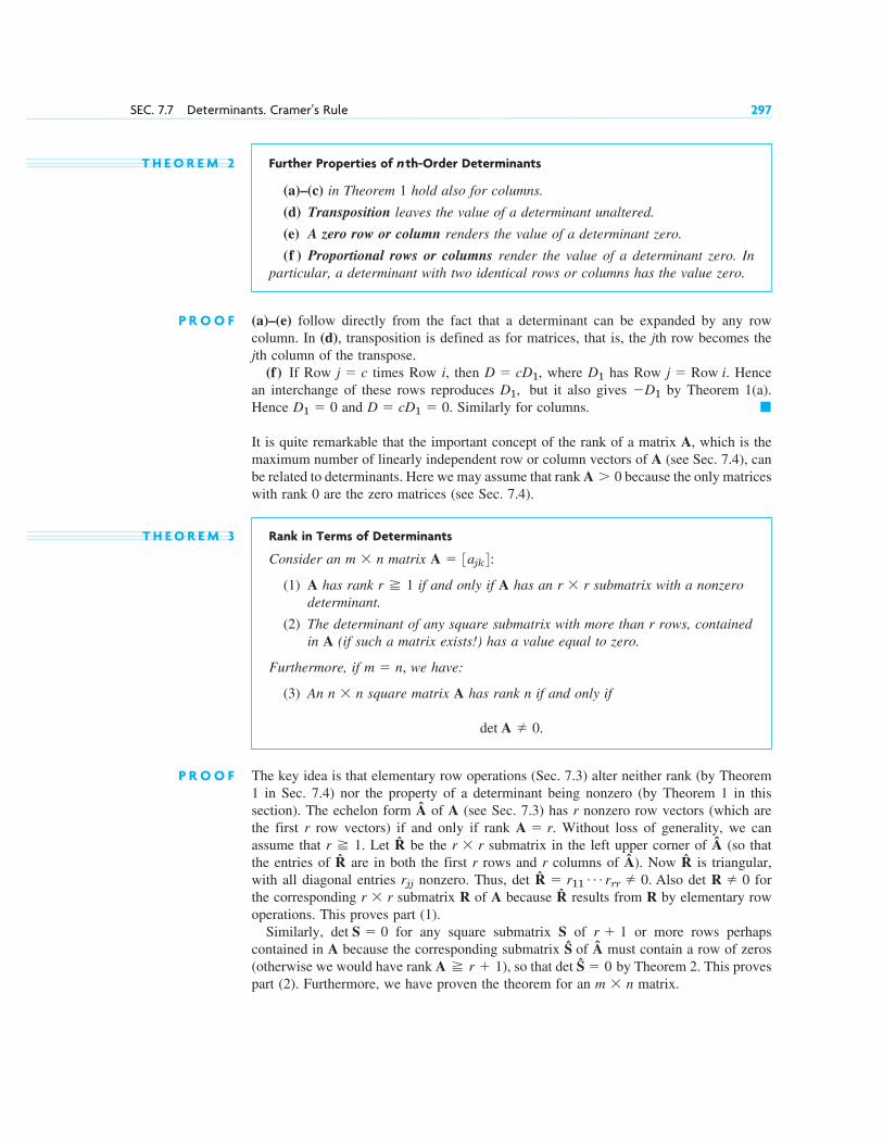
T H E O R E M 2 Further Properties of nth-Order Determinants
(a)–(c) in Theorem 1 hold also for columns.
(d) Transposition leaves the value of a determinant unaltered.
(e) A zero row or column renders the value of a determinant zero.
(f ) Proportional rows or columns render the value of a determinant zero. Inparticular, a determinant with two identical rows or columns has the value zero.
P R O O F (a)–(e) follow directly from the fact that a determinant can be expanded by any rowcolumn. In (d), transposition is defined as for matrices, that is, the jth row becomes thejth column of the transpose.
(f) If Row times Row i, then , where has Row Hencean interchange of these rows reproduces but it also gives by Theorem 1(a).Hence and Similarly for columns.
It is quite remarkable that the important concept of the rank of a matrix A, which is themaximum number of linearly independent row or column vectors of A (see Sec. 7.4), canbe related to determinants. Here we may assume that rank because the only matriceswith rank 0 are the zero matrices (see Sec. 7.4).
T H E O R E M 3 Rank in Terms of Determinants
Consider an matrix :
(1) A has rank if and only if A has an submatrix with a nonzerodeterminant.
(2) The determinant of any square submatrix with more than r rows, containedin A (if such a matrix exists!) has a value equal to zero.
Furthermore, if , we have:
(3) An square matrix A has rank n if and only if
P R O O F The key idea is that elementary row operations (Sec. 7.3) alter neither rank (by Theorem1 in Sec. 7.4) nor the property of a determinant being nonzero (by Theorem 1 in thissection). The echelon form  of A (see Sec. 7.3) has r nonzero row vectors (which arethe first r row vectors) if and only if rank Without loss of generality, we canassume that Let R be the submatrix in the left upper corner of  (so thatthe entries of R are in both the first r rows and r columns of Â). Now R is triangular,with all diagonal entries nonzero. Thus, det R Also det forthe corresponding submatrix R of A because R results from R by elementary rowoperations. This proves part (1).
Similarly, for any square submatrix S of or more rows perhapscontained in A because the corresponding submatrix S of  must contain a row of zeros(otherwise we would have rank ), so that det S by Theorem 2. This provespart (2). Furthermore, we have proven the theorem for an matrix.m � n
� 0A r � 1
r � 1det S � 0
r � rR � 0� r11
Á rrr � 0.rjj
r � rr 1.A � r.
det A � 0.
n � n
m � n
r � rr 1
A � 3ajk4m � n
A � 0
�D � cD1 � 0.D1 � 0�D1D1,
j � Row i.D1D � cD1j � c
SEC. 7.7 Determinants. Cramer’s Rule 297

For an square matrix A we proceed as follows. To prove (3), we apply part (1)(already proven!). This gives us that rank if and only if A contains an submatrix with nonzero determinant. But the only such submatrix contained in our squarematrix A, is A itself, hence This proves part (3).
Cramer’s RuleTheorem 3 opens the way to the classical solution formula for linear systems known asCramer’s rule,2 which gives solutions as quotients of determinants. Cramer’s rule is notpractical in computations for which the methods in Secs. 7.3 and 20.1–20.3 are suitable.However, Cramer’s rule is of theoretical interest in differential equations (Secs. 2.10 and3.3) and in other theoretical work that has engineering applications.
T H E O R E M 4 Cramer’s Theorem (Solution of Linear Systems by Determinants)
(a) If a linear system of n equations in the same number of unknowns
(6)
has a nonzero coefficient determinant the system has precisely onesolution. This solution is given by the formulas
(7)
where is the determinant obtained from D by replacing in D the kth column bythe column with the entries
(b) Hence if the system (6) is homogeneous and it has only the trivialsolution If the homogeneous system also hasnontrivial solutions.
P R O O F The augmented matrix A� of the system (6) is of size n � (n � 1). Hence its rank can beat most n. Now if
(8) D � det A � 5 a11Á a1n
# Á #
# Á #
an1Á ann
5 � 0,
D � 0,x1 � 0, x2 � 0, Á , xn � 0.D � 0,
b1, Á , bn.Dk
(Cramer’s rule)x1 �D1
D , x2 �
D2
D , Á , xn �
Dn
D
D � det A,
a11x1 � a12x2 � Á � a1nxn � b1
a21x1 � a22x2 � Á � a2nxn � b2
# # # # # # # # # # # # # # # # #
an1x1 � an2x2 � Á � annxn � bn
x1, Á , xn
�det A � 0.
n � nA � n 1n � n
298 CHAP. 7 Linear Algebra: Matrices, Vectors, Determinants. Linear Systems
2GABRIEL CRAMER (1704–1752), Swiss mathematician.

then rank by Theorem 3. Thus rank . Hence, by the FundamentalTheorem in Sec. 7.5, the system (6) has a unique solution.
Let us now prove (7). Expanding D by its kth column, we obtain
(9)
where is the cofactor of entry in D. If we replace the entries in the kth column ofD by any other numbers, we obtain a new determinant, say, D. Clearly, its expansion bythe kth column will be of the form (9), with replaced by those new numbersand the cofactors as before. In particular, if we choose as new numbers the entries
of the lth column of D (where ), we have a new determinant D whichhas the column twice, once as its lth column, and once as its kth becauseof the replacement. Hence D by Theorem 2(f). If we now expand D by the columnthat has been replaced (the kth column), we thus obtain
(10)
We now multiply the first equation in (6) by on both sides, the second by the last by and add the resulting equations. This gives
(11)
Collecting terms with the same xj, we can write the left side as
From this we see that is multiplied by
Equation (9) shows that this equals D. Similarly, is multiplied by
Equation (10) shows that this is zero when Accordingly, the left side of (11) equalssimply so that (11) becomes
Now the right side of this is as defined in the theorem, expanded by its kth column,so that division by D gives (7). This proves Cramer’s rule.
If (6) is homogeneous and , then each has a column of zeros, so that by Theorem 2(e), and (7) gives the trivial solution.
Finally, if (6) is homogeneous and then rank by Theorem 3, so thatnontrivial solutions exist by Theorem 2 in Sec. 7.5.
E X A M P L E 5 Illustration of Cramer’s Rule (Theorem 4)
For see Example 1 of Sec. 7.6. Also, at the end of that section, we give Cramer’s rule for a generallinear system of three equations. �
n � 2,
�
A nD � 0,
Dk � 0DkD � 0
Dk
xkD � b1C1k � b2C2k � Á � bnCnk.
xkD,l � k.
a1lC1k � a2lC2k � Á � anlCnk.
x1
a1kC1k � a2kC2k � Á � ankCnk.
xk
x1(a11C1k � a21C2k � Á � an1Cnk) � Á � xn(a1nC1k � a2nC2k � Á � annCnk).
� b1C1k � Á � bnCnk.
C1k(a11x1 � Á � a1nxn) � Á � Cnk(an1x1 � Á � annxn)
Cnk,C2k, Á , C1k
(l � k).a1lC1k � a2lC2k � Á � anlCnk � 0
� 03a1l Á anl4
Tl � ka1l, Á , anl
Cik
a1k, Á , ank
aikCik
D � a1kC1k � a2kC2k � Á � ankCnk,
A~ � rank AA � n
SEC. 7.7 Determinants. Cramer’s Rule 299

Finally, an important application for Cramer’s rule dealing with inverse matrices willbe given in the next section.
300 CHAP. 7 Linear Algebra: Matrices, Vectors, Determinants. Linear Systems
1–6 GENERAL PROBLEMS1. General Properties of Determinants. Illustrate each
statement in Theorems 1 and 2 with an example ofyour choice.
2. Second-Order Determinant. Expand a generalsecond-order determinant in four possible ways andshow that the results agree.
3. Third-Order Determinant. Do the task indicated inTheorem 2. Also evaluate D by reduction to triangularform.
4. Expansion Numerically Impractical. Show that thecomputation of an nth-order determinant by expansioninvolves multiplications, which if a multiplicationtakes sec would take these times:
n 10 15 20 25
Time0.004 22 77sec min years years
5. Multiplication by Scalar. Show that (not k det A). Give an example.
6. Minors, cofactors. Complete the list in Example 1.
7–15 EVALUATION OF DETERMINANTSShowing the details, evaluate:
7. 8.
9. 10.
11. 12.
13. 14. 6 4 7 0 0
2 8 0 0
0 0 1 5
0 0 �2 2
66 0 4 �1 5
�4 0 3 �2
1 �3 0 1
�5 2 �1 0
6
3 a b c
c a b
b c a
33 4 �1 8
0 2 3
0 0 5
32 cosh t sinh t
sinh t cosh t 22 cos nu sin nu
�sin nu cos nu 2
2 0.4 4.9
1.5 �1.3 22 cos a sin a
sin b cos b 2
kn det Adet (kA) �
0.5 # 109
10�9n!
P R O B L E M S E T 7 . 7
15.
16. CAS EXPERIMENT. Determinant of Zeros andOnes. Find the value of the determinant of the matrix with main diagonal entries all 0 and allothers 1. Try to find a formula for this. Try to prove itby induction. Interpret and as incidence matrices(as in Problem Set 7.1 but without the minuses) of atriangle and a tetrahedron, respectively; similarly for ann-simplex, having n vertices and edges (andspanning ).
17–19 RANK BY DETERMINANTSFind the rank by Theorem 3 (which is not very practical)and check by row reduction. Show details.
17. 18.
19.
20. TEAM PROJECT. Geometric Applications: Curvesand Surfaces Through Given Points. The idea is toget an equation from the vanishing of the determinantof a homogeneous linear system as the condition for anontrivial solution in Cramer’s theorem. We explainthe trick for obtaining such a system for the case ofa line L through two given points and
The unknown line issay. We write it as To get anontrivial solution a, b, c, the determinant of the“coefficients” x, y, 1 must be zero. The system is
(12)
ax2 � by2 � c # 1 � 0 (P2 on L).
ax1 � by1 � c # 1 � 0 (P1 on L)
ax � by � c # 1 � 0 (Line L)
ax � by � c # 1 � 0.ax � by � �c,P2: (x2, y2).P1: (x1, y1)
D
1 5 2 2
1 3 2 6
4 0 8 48
TD
0 4 �6
4 0 10
�6 10 0
TD
4 9
�8 �6
16 12
T
Rn�1, n � 5, 6, Án (n � 1)>2
A4A3
An
n � n
6 1 2 0 0
2 4 2 0
0 2 9 2
0 0 2 16
6

(a) Line through two points. Derive from in(12) the familiar formula
(b) Plane. Find the analog of (12) for a plane throughthree given points. Apply it when the points are
(c) Circle. Find a similar formula for a circle in theplane through three given points. Find and sketch thecircle through (d) Sphere. Find the analog of the formula in (c) fora sphere through four given points. Find the spherethrough by thisformula or by inspection.(e) General conic section. Find a formula for ageneral conic section (the vanishing of a determinantof 6th order). Try it out for a quadratic parabola andfor a more general conic section of your own choice.
(0, 0, 5), (4, 0, 1), (0, 4, 1), (0, 0, �3)
(2, 6), (6, 4), (7, 1).
(1, 1, 1), (3, 2, 6), (5, 0, 5).
x � x1
x1 � x2 �
y � y1
y1 � y2.
D � 0
SEC. 7.8 Inverse of a Matrix. Gauss–Jordan Elimination 301
21–25 CRAMER’S RULESolve by Cramer’s rule. Check by Gauss elimination andback substitution. Show details.
21. 22.
23. 24.
25. �4w � x � y � �10
w � 4x � z � 1
w � 4y � z � �7
x � y � 4z � 10
3x � 2y � z � 13
�2x � y � 4z � 11
x � 4y � 5z � �31
3y � 4z � 16
2x � 5y � 7z � �27
�x � 9z � 9
2x � 4y � �24
5x � 2y � 0
3x � 5y � 15.5
6x � 16y � 5.0
7.8 Inverse of a Matrix.Gauss–Jordan Elimination
In this section we consider square matrices exclusively.The inverse of an matrix is denoted by and is an matrix
such that
(1)
where I is the unit matrix (see Sec. 7.2).If A has an inverse, then A is called a nonsingular matrix. If A has no inverse, then
A is called a singular matrix.If A has an inverse, the inverse is unique.Indeed, if both B and C are inverses of A, then and so that we obtain
the uniqueness from
We prove next that A has an inverse (is nonsingular) if and only if it has maximumpossible rank n. The proof will also show that implies provided exists, and will thus give a motivation for the inverse as well as a relation to linear systems.(But this will not give a good method of solving numerically because the Gausselimination in Sec. 7.3 requires fewer computations.)
T H E O R E M 1 Existence of the Inverse
The inverse of an matrix A exists if and only if , thus (byTheorem 3, Sec. 7.7) if and only if . Hence A is nonsingular ifand is singular if .rank A n
rank A � n,det A � 0rank A � nn � nA�1
Ax � b
A�1x � A�1bAx � b
B � IB � (CA)B � C(AB) � CI � C.
CA � I, AB � I
n � n
AA�1 � A�1A � I
n � nA�1A � 3ajk4n � n

302 CHAP. 7 Linear Algebra: Matrices, Vectors, Determinants. Linear Systems
P R O O F Let A be a given matrix and consider the linear system
(2)
If the inverse exists, then multiplication from the left on both sides and use of (1)gives
.
This shows that (2) has a solution x, which is unique because, for another solution u, wehave , so that . Hence A must have rank n by the FundamentalTheorem in Sec. 7.5.
Conversely, let rank . Then by the same theorem, the system (2) has a uniquesolution x for any b. Now the back substitution following the Gauss elimination (Sec. 7.3)shows that the components of x are linear combinations of those of b. Hence we canwrite
(3)
with B to be determined. Substitution into (2) gives
for any b. Hence , the unit matrix. Similarly, if we substitute (2) into (3) we get
for any x (and ). Hence . Together, exists.
Determination of the Inverse by the Gauss–Jordan MethodTo actually determine the inverse of a nonsingular matrix A, we can use avariant of the Gauss elimination (Sec. 7.3), called the Gauss–Jordan elimination.3 Theidea of the method is as follows.
Using A, we form n linear systems
where the vectors are the columns of the unit matrix I; thus,etc. These are n vector equations
in the unknown vectors . We combine them into a single matrix equationx(1), Á , x(n)
e(1) � 31 0 Á 04T, e(2) � 30 1 0 Á 04T, n � ne(1), Á , e(n)
Ax(1) � e(1), Á , Ax(n) � e(n)
n � nA�1
�B � A�1BA � Ib � Ax
x � Bb � B(Ax) � (BA)x
C � AB � I
(C � AB)Ax � A(Bb) � (AB)b � Cb � b
x � Bb
x j
A � n
u � A�1b � xAu � b
A�1Ax � x � A�1b
A�1
Ax � b.
n � n
3WILHELM JORDAN (1842–1899), German geodesist and mathematician. He did important geodesic workin Africa, where he surveyed oases. [See Althoen, S.C. and R. McLaughlin, Gauss–Jordan reduction: A briefhistory. American Mathematical Monthly, Vol. 94, No. 2 (1987), pp. 130–142.]
We do not recommend it as a method for solving systems of linear equations, since the number of operationsin addition to those of the Gauss elimination is larger than that for back substitution, which the Gauss–Jordanelimination avoids. See also Sec. 20.1.

, with the unknown matrix X having the columns Correspondingly,we combine the n augmented matrices into one wide “augmented matrix” . Now multiplication of by from the leftgives Hence, to solve for X, we can apply the Gausselimination to . This gives a matrix of the form with upper triangularU because the Gauss elimination triangularizes systems. The Gauss–Jordan methodreduces U by further elementary row operations to diagonal form, in fact to the unit matrixI. This is done by eliminating the entries of U above the main diagonal and making thediagonal entries all 1 by multiplication (see Example 1). Of course, the method operateson the entire matrix , transforming H into some matrix K, hence the entire to . This is the “augmented matrix” of . Now , as shownbefore. By comparison, , so that we can read directly from .
The following example illustrates the practical details of the method.
E X A M P L E 1 Finding the Inverse of a Matrix by Gauss–Jordan Elimination
Determine the inverse of
Solution. We apply the Gauss elimination (Sec. 7.3) to the following matrix, where BLUEalways refers to the previous matrix.
This is as produced by the Gauss elimination. Now follow the additional Gauss–Jordan steps, reducingU to I, that is, to diagonal form with entries 1 on the main diagonal.
D1 0 0
0 1 0
0 0 1
3
�0.7 0.2 0.3
�1.3 �0.2 0.7
0.8 0.2 �0.2
T Row 1 � Row 2
D1 �1 0
0 1 0
0 0 1
3
0.6 0.4 �0.4
�1.3 �0.2 0.7
0.8 0.2 �0.2
T Row 1 � 2 Row 3
Row 2 – 3.5 Row 3
D1 �1 �2
0 1 3.5
0 0 1
3
�1 0 0
1.5 0.5 0
0.8 0.2 �0.2
T �Row 1
0.5 Row 2
�0.2 Row 3
3U H4
D�1 1 2
0 2 7
0 0 �5
3 1 0 0
3 1 0
�4 �1 1
T Row 3 � Row 2
D�1 1 2
0 2 7
0 2 2
3
1 0 0
3 1 0
�1 0 1
T Row 2 � 3 Row 1
Row 3 � Row 1
3A I4 � D�1 1 2
3 �1 1
�1 3 4
3
1 0 0
0 1 0
0 0 1
Tn � 2n � 3 � 6
A � D�1 1 2
3 �1 1
�1 3 4
T .
A�1
3I K4A�1K � A�1IX � X � A�1IX � K3I K4
3U H43U H4
3U H4A� � 3A I4AX � IX � A�1I � A�1.
A�1AX � IA� � 3A I4n � 2n3A e(1)4, Á , 3A e(n)4
x(1), Á , x(n).AX � I
SEC. 7.8 Inverse of a Matrix. Gauss–Jordan Elimination 303

The last three columns constitute Check:
Hence Similarly,
Formulas for InversesSince finding the inverse of a matrix is really a problem of solving a system of linearequations, it is not surprising that Cramer’s rule (Theorem 4, Sec. 7.7) might come intoplay. And similarly, as Cramer’s rule was useful for theoretical study but not forcomputation, so too is the explicit formula (4) in the following theorem useful fortheoretical considerations but not recommended for actually determining inverse matrices,except for the frequently occurring case as given in
T H E O R E M 2 Inverse of a Matrix by Determinants
The inverse of a nonsingular matrix is given by
(4)
where is the cofactor of in det A (see Sec. 7.7). (CAUTION! Note well thatin , the cofactor occupies the same place as (not ) does in A.)
In particular, the inverse of
P R O O F We denote the right side of (4) by B and show that . We first write
(5)
and then show that . Now by the definition of matrix multiplication and because ofthe form of B in (4), we obtain (CAUTION! not )
(6) gkl � a
n
s�1
Csk
det A asl �
1det A
(a1lC1k � Á � anlCnk).
CksCsk, G � I
BA � G � 3gkl4
BA � I
A � ca11 a12
a21 a22
d is A�1 �1
det A c a22 �a12
�a21 a11
d .(4*)
ajkakjCjkA�1ajkCjk
A�1 �1
det A 3Cjk4
T �1
det A EC11 C21
Á Cn1
C12 C22Á Cn2
# # Á #
C1n C2nÁ Cnn
U ,
A � 3ajk4n � n
(4*).2 � 2
�A�1A � I.AA�1 � I.
D�1 1 2
3 �1 1
�1 3 4
T D�0.7 0.2 0.3
�1.3 �0.2 0.7
0.8 0.2 �0.2
T � D1 0 0
0 1 0
0 0 1
T .
A�1.
304 CHAP. 7 Linear Algebra: Matrices, Vectors, Determinants. Linear Systems

Now (9) and (10) in Sec. 7.7 show that the sum on the right is when, and is zero when . Hence
In particular, for we have in (4), in the first row, and, in the second row, This gives
The special case occurs quite frequently in geometric and other applications. Youmay perhaps want to memorize formula (4*). Example 2 gives an illustration of (4*).
E X A M P L E 2 Inverse of a Matrix by Determinants
E X A M P L E 3 Further Illustration of Theorem 2
Using (4), find the inverse of
Solution. We obtain and in (4),
so that by (4), in agreement with Example 1,
Diagonal matrices when have an inverse if and only if allThen is diagonal, too, with entries
P R O O F For a diagonal matrix we have in (4)
etc. �C11
D�
a22Á ann
a11a22Á ann
�1
a11,
1>a11, Á , 1>ann.A�1ajj � 0.j � k, A � [ajk], ajk � 0
�A�1 � D�0.7 0.2 0.3
�1.3 �0.2 0.7
0.8 0.2 �0.2
T .
C13 � 2 3 �1
�1 3 2 � 8, C23 � � 2 �1 1
�1 3 2 � 2, C33 � 2 �1 1
3 �1 2 � �2,
C12 � � 2 3 1
�1 4 2 � �13, C22 � 2 �1 2
�1 4 2 � �2, C32 � � 2 �1 2
3 1 2 � 7,
C11 � 2 �1 1
3 4 2 � �7, C21 � � 2 1 2
3 4 2 � 2, C31 � 2 1 2
�1 1 2 � 3,
det A � �1(�7) � 1 # 13 � 2 # 8 � 10,
A � D�1 1 2
3 �1 1
�1 3 4
T .
�A � c3 1
2 4d , A�1 �
1
10 c 4 �1
�2 3d � c 0.4 �0.1
�0.2 0.3d
2 � 2
n � 2
�(4*).C12 � �a21, C22 � a11.C11 � a22, C21 � �a12n � 2
gkl � 0 (l � k).
gkk �1
det A det A � 1,
l � kl � kD � det A( Á )
SEC. 7.8 Inverse of a Matrix. Gauss–Jordan Elimination 305

E X A M P L E 4 Inverse of a Diagonal Matrix
Let
Then we obtain the inverse by inverting each individual diagonal element of A, that is, by taking and as the diagonal entries of , that is,
Products can be inverted by taking the inverse of each factor and multiplying theseinverses in reverse order,
(7)
Hence for more than two factors,
(8)
P R O O F The idea is to start from (1) for AC instead of A, that is, , and multiplyit on both sides from the left, first by which because of gives
and then multiplying this on both sides from the left, this time by and by using
This proves (7), and from it, (8) follows by induction.
We also note that the inverse of the inverse is the given matrix, as you may prove,
(9)
Unusual Properties of Matrix Multiplication.Cancellation LawsSection 7.2 contains warnings that some properties of matrix multiplication deviate fromthose for numbers, and we are now able to explain the restricted validity of the so-calledcancellation laws [2] and [3] below, using rank and inverse, concepts that were not yet
(A�1)�1 � A.
�
C�1C(AC)�1 � (AC)�1 � C�1A�1.
C�1C � I, C�1
� A�1I � A�1,
A�1AC(AC)�1 � C(AC)�1
A�1A � IA�1, AC(AC)�1 � I
(AC Á PQ)�1 � Q�1P�1 Á C�1A�1.
(AC)�1 � C�1A�1.
�A�1 � D�2 0 0
0 0.25 0
0 0 1
T .
A�111
1>(�0.5), 14 ,A�1
A � D�0.5 0 0
0 4 0
0 0 1
T .
306 CHAP. 7 Linear Algebra: Matrices, Vectors, Determinants. Linear Systems

SEC. 7.8 Inverse of a Matrix. Gauss–Jordan Elimination 307
available in Sec. 7.2. The deviations from the usual are of great practical importance andmust be carefully observed. They are as follows.
[1] Matrix multiplication is not commutative, that is, in general we have
[2] does not generally imply or (or ); for example,
[3] does not generally imply (even when
Complete answers to [2] and [3] are contained in the following theorem.
T H E O R E M 3 Cancellation Laws
Let A, B, C be matrices. Then:
(a) If rank and , then
(b) If rank , then implies . Hence if , butas well as , then rank and rank
(c) If A is singular, so are BA and AB.
P R O O F (a) The inverse of A exists by Theorem 1. Multiplication by from the left gives, hence .
(b) Let rank . Then exists, and implies Similarlywhen rank . This implies the second statement in (b).
Rank by Theorem 1. Hence has nontrivial solutions by Theorem 2in Sec. 7.5. Multiplication by B shows that these solutions are also solutions of so that rank by Theorem 2 in Sec. 7.5 and BA is singular by Theorem 1.
is singular by Theorem 2(d) in Sec. 7.7. Hence is singular by part ,and is equal to by (10d) in Sec. 7.2. Hence AB is singular by Theorem 2(d) inSec. 7.7.
Determinants of Matrix ProductsThe determinant of a matrix product AB or BA can be written as the product of thedeterminants of the factors, and it is interesting that , although in general. The corresponding formula (10) is needed occasionally and can be obtainedby Gauss–Jordan elimination (see Example 1) and from the theorem just proved.
T H E O R E M 4 Determinant of a Product of Matrices
For any matrices A and B,
(10) .det (AB) � det (BA) � det A det B
n � n
AB � BAdet AB � det BA
�
(AB)T(c1)BTATAT(c2)
(BA) nBAx � 0,
Ax � 0A n(c1)B � n
A�1AB � B � 0.AB � 0A�1A � nB � CA�1AB � A�1AC
A�1
B n.A nB � 0A � 0AB � 0B � 0AB � 0A � n
B � C.AB � ACA � n
n � n
A � 0).C � DAC � AD
c1 1
2 2d c�1 1
1 �1d � c0 0
0 0d .BA � 0B � 0A � 0AB � 0
AB � BA.
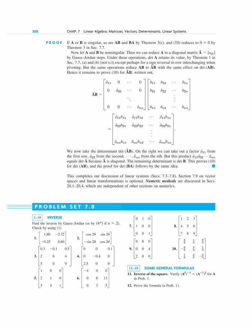
308 CHAP. 7 Linear Algebra: Matrices, Vectors, Determinants. Linear Systems
P R O O F If A or B is singular, so are AB and BA by Theorem 3(c), and (10) reduces to byTheorem 3 in Sec. 7.7.
Now let A and B be nonsingular. Then we can reduce A to a diagonal matrix Âby Gauss–Jordan steps. Under these operations, det A retains its value, by Theorem 1 inSec. 7.7, (a) and (b) [not (c)] except perhaps for a sign reversal in row interchanging whenpivoting. But the same operations reduce AB to ÂB with the same effect on .Hence it remains to prove (10) for ÂB; written out,
Â
We now take the determinant (ÂB). On the right we can take out a factor fromthe first row, from the second, from the nth. But this product equals  because  is diagonal. The remaining determinant is . This proves (10)for , and the proof for follows by the same idea.
This completes our discussion of linear systems (Secs. 7.3–7.8). Section 7.9 on vectorspaces and linear transformations is optional. Numeric methods are discussed in Secs.20.1–20.4, which are independent of other sections on numerics.
�det (BA)det (AB)det Bdet
a11a22Á ann
Á , a ˆnna22
a11det
� E a11b11 a11b12Á a11b1n
a22b21 a22b22Á a22b2n
.
.
.
annbn1 annbn2Á annbnn
U .
B � Ea11 0 Á 0
0 a22Á 0
. . .
0 0 Á ann
U Eb11 b12Á b1n
b21 b22Á b2n
.
.
.
bn1 bn2Á bnn
Udet (AB)
� [ajk]
0 � 0
1–10 INVERSEFind the inverse by Gauss–Jordan (or by if ).Check by using (1).
1. 2.
3. 4.
5. 6. D�4 0 0
0 8 13
0 3 5
TD1 0 0
2 1 0
5 4 1
TD0 0 0.1
0 �0.4 0
2.5 0 0
TD0.3 �0.1 0.5
2 6 4
5 0 9
Tc cos 2u sin 2u
�sin 2u cos 2udc 1.80 �2.32
�0.25 0.60d
n � 2(4*)7. 8.
9. 10.
11–18 SOME GENERAL FORMULAS11. Inverse of the square. Verify for A
in Prob. 1.
12. Prove the formula in Prob. 11.
(A2)�1 � (A�1)2
D 23
13
23
�23
23
13
13
23 �2
3
TD0 8 0
0 0 4
2 0 0
TD1 2 3
4 5 6
7 8 9
TD0 1 0
1 0 0
0 0 1
TP R O B L E M S E T 7 . 8

13. Inverse of the transpose. Verify forA in Prob. 1.
14. Prove the formula in Prob. 13.
15. Inverse of the inverse. Prove that
16. Rotation. Give an application of the matrix in Prob. 2that makes the form of the inverse obvious.
17. Triangular matrix. Is the inverse of a triangularmatrix always triangular (as in Prob. 5)? Give reason.
(A�1)�1 � A.
(AT)�1 � (A�1)T
SEC. 7.9 Vector Spaces, Inner Product Spaces, Linear Transformations Optional 309
18. Row interchange. Same task as in Prob. 16 for thematrix in Prob. 7.
19–20 FORMULA (4) Formula (4) is occasionally needed in theory. To understandit, apply it and check the result by Gauss–Jordan:
19. In Prob. 3
20. In Prob. 6
7.9 Vector Spaces, Inner Product Spaces, Linear Transformations Optional
We have captured the essence of vector spaces in Sec. 7.4. There we dealt with specialvector spaces that arose quite naturally in the context of matrices and linear systems. Theelements of these vector spaces, called vectors, satisfied rules (3) and (4) of Sec. 7.1(which were similar to those for numbers). These special vector spaces were generatedby spans, that is, linear combination of finitely many vectors. Furthermore, each suchvector had n real numbers as components. Review this material before going on.
We can generalize this idea by taking all vectors with n real numbers as componentsand obtain the very important real n-dimensional vector space . The vectors are knownas “real vectors.” Thus, each vector in is an ordered n-tuple of real numbers.
Now we can consider special values for n. For , we obtain the vector spaceof all ordered pairs, which correspond to the vectors in the plane. For , we obtain
the vector space of all ordered triples, which are the vectors in 3-space. These vectorshave wide applications in mechanics, geometry, and calculus and are basic to the engineerand physicist.
Similarly, if we take all ordered n-tuples of complex numbers as vectors and complexnumbers as scalars, we obtain the complex vector space , which we shall consider inSec. 8.5.
Furthermore, there are other sets of practical interest consisting of matrices, functions,transformations, or others for which addition and scalar multiplication can be defined inan almost natural way so that they too form vector spaces.
It is perhaps not too great an intellectual jump to create, from the concrete modelthe abstract concept of a real vector space V by taking the basic properties (3) and (4)in Sec. 7.1 as axioms. In this way, the definition of a real vector space arises.
D E F I N I T I O N Real Vector Space
A nonempty set V of elements a, b, • • • is called a real vector space (or real linearspace), and these elements are called vectors (regardless of their nature, which willcome out from the context or will be left arbitrary) if, in V, there are defined twoalgebraic operations (called vector addition and scalar multiplication) as follows.
I. Vector addition associates with every pair of vectors a and b of V a uniquevector of V, called the sum of a and b and denoted by a � b, such that the followingaxioms are satisfied.
Rn,
C n
R3, n � 3
R2, n � 2Rn
Rn

310 CHAP. 7 Linear Algebra: Matrices, Vectors, Determinants. Linear Systems
I.1 Commutativity. For any two vectors a and b of V,
a � b � b � a.
I.2 Associativity. For any three vectors a, b, c of V,
(a � b) � c � a � (b � c) (written a � b � c).
I.3 There is a unique vector in V, called the zero vector and denoted by 0, suchthat for every a in V,
a � 0 � a.
I.4 For every a in V there is a unique vector in V that is denoted by �a and issuch that
a � (�a) � 0.
II. Scalar multiplication. The real numbers are called scalars. Scalarmultiplication associates with every a in V and every scalar c a unique vector of V,called the product of c and a and denoted by ca (or ac) such that the followingaxioms are satisfied.
II.1 Distributivity. For every scalar c and vectors a and b in V,
c (a � b) � ca � cb.
II.2 Distributivity. For all scalars c and k and every a in V,
(c � k)a � ca � ka.
II.3 Associativity. For all scalars c and k and every a in V,
c(ka) � (ck)a (written cka).
II.4 For every a in V,
1a � a.
If, in the above definition, we take complex numbers as scalars instead of real numbers,we obtain the axiomatic definition of a complex vector space.
Take a look at the axioms in the above definition. Each axiom stands on its own: Itis concise, useful, and it expresses a simple property of V. There are as few axioms aspossible and together they express all the desired properties of V. Selecting good axiomsis a process of trial and error that often extends over a long period of time. But onceagreed upon, axioms become standard such as the ones in the definition of a real vectorspace.

The following concepts related to a vector space are exactly defined as those given inSec. 7.4. Indeed, a linear combination of vectors in a vector space V is anexpression
any scalars).
These vectors form a linearly independent set (briefly, they are called linearlyindependent) if
(1)
implies that . Otherwise, if (1) also holds with scalars not all zero, thevectors are called linearly dependent.
Note that (1) with is and shows that a single vector a is linearlyindependent if and only if .
V has dimension n, or is n-dimensional, if it contains a linearly independent set of nvectors, whereas any set of more than n vectors in V is linearly dependent. That set ofn linearly independent vectors is called a basis for V. Then every vector in V can bewritten as a linear combination of the basis vectors. Furthermore, for a given basis, thisrepresentation is unique (see Prob. 2).
E X A M P L E 1 Vector Space of Matrices
The real matrices form a four-dimensional real vector space. A basis is
because any matrix has a unique representation .Similarly, the real matrices with fixed m and n form an mn-dimensional vector space. What is thedimension of the vector space of all skew-symmetric matrices? Can you find a basis?
E X A M P L E 2 Vector Space of Polynomials
The set of all constant, linear, and quadratic polynomials in x together is a vector space of dimension 3 withbasis under the usual addition and multiplication by real numbers because these two operations givepolynomials not exceeding degree 2. What is the dimension of the vector space of all polynomials of degreenot exceeding a given fixed n? Can you find a basis?
If a vector space V contains a linearly independent set of n vectors for every n, no matterhow large, then V is called infinite dimensional, as opposed to a finite dimensional(n-dimensional) vector space just defined. An example of an infinite dimensional vectorspace is the space of all continuous functions on some interval [a, b] of the x-axis, as wemention without proof.
Inner Product SpacesIf a and b are vectors in , regarded as column vectors, we can form the product .This is a matrix, which we can identify with its single entry, that is, with a number.1 � 1
aTbRn
�
{1, x, x2}
�3 � 3m � n
A � a11B11 � a12B12 � a21B21 � a22B22A � [ajk]2 � 2
B11 � c1 0
0 0d , B12 � c0 1
0 0d , B21 � c0 0
1 0d , B22 � c0 0
0 1d
2 � 2
a � 0ca � 0m � 1
c1 � 0, Á , cm � 0
c1a(1) � Á � cma(m) � 0
(c1, Á , cmc1a(1) � Á � cmam
a(1), Á , a(m)
SEC. 7.9 Vector Spaces, Inner Product Spaces, Linear Transformations Optional 311

This product is called the inner product or dot product of a and b. Other notations forit are (a, b) and . Thus
.
We now extend this concept to general real vector spaces by taking basic properties of(a, b) as axioms for an “abstract inner product” (a, b) as follows.
D E F I N I T I O N Real Inner Product Space
A real vector space V is called a real inner product space (or real pre-Hilbert4
space) if it has the following property. With every pair of vectors a and b in V thereis associated a real number, which is denoted by (a, b) and is called the innerproduct of a and b, such that the following axioms are satisfied.
I. For all scalars q1 and q2 and all vectors a, b, c in V,
(Linearity).
II. For all vectors a and b in V,
(Symmetry).
III. For every a in V,
(Positive-definiteness).
Vectors whose inner product is zero are called orthogonal.The length or norm of a vector in V is defined by
(2) .
A vector of norm 1 is called a unit vector.
� a � � 2(a, a) ( 0)
(a, a) 0,
(a, a) � 0 if and only if a � 0 r
(a, b) � (b, a)
(q1a � q2b, c) � q1(a, c) � q2(b, c)
aTb � (a, b) � a • b � 3a1Á an4 Db1
o
bn
T � a
n
i�1
albl � a1b1 � Á � anbn
a • b
312 CHAP. 7 Linear Algebra: Matrices, Vectors, Determinants. Linear Systems
4DAVID HILBERT (1862–1943), great German mathematician, taught at Königsberg and Göttingen and wasthe creator of the famous Göttingen mathematical school. He is known for his basic work in algebra, the calculusof variations, integral equations, functional analysis, and mathematical logic. His “Foundations of Geometry”helped the axiomatic method to gain general recognition. His famous 23 problems (presented in 1900 at theInternational Congress of Mathematicians in Paris) considerably influenced the development of modernmathematics.
If V is finite dimensional, it is actually a so-called Hilbert space; see [GenRef7], p. 128, listed in App. 1.

From these axioms and from (2) one can derive the basic inequality
(3) (Cauchy–Schwarz5 inequality).
From this follows
(4) (Triangle inequality).
A simple direct calculation gives
(5) (Parallelogram equality).
E X A M P L E 3 n-Dimensional Euclidean Space
with the inner product
(6)
(where both a and b are column vectors) is called the n-dimensional Euclidean space and is denoted by oragain simply by . Axioms I–III hold, as direct calculation shows. Equation (2) gives the “Euclidean norm”
(7) .
E X A M P L E 4 An Inner Product for Functions. Function Space
The set of all real-valued continuous functions on a given interval is a real vectorspace under the usual addition of functions and multiplication by scalars (real numbers). On this “functionspace” we can define an inner product by the integral
(8)
Axioms I–III can be verified by direct calculation. Equation (2) gives the norm
(9)
Our examples give a first impression of the great generality of the abstract concepts ofvector spaces and inner product spaces. Further details belong to more advanced courses(on functional analysis, meaning abstract modern analysis; see [GenRef7] listed in App.1) and cannot be discussed here. Instead we now take up a related topic where matricesplay a central role.
Linear TransformationsLet X and Y be any vector spaces. To each vector x in X we assign a unique vector y inY. Then we say that a mapping (or transformation or operator) of X into Y is given.Such a mapping is denoted by a capital letter, say F. The vector y in Y assigned to a vectorx in X is called the image of x under F and is denoted by [or Fx, without parentheses].F (x)
�� f � � 2( f, f ) �G �b
a
f (x)2 dx.
( f, g) � �b
a
f (x) g (x) dx.
a � x � bf (x), g (x), Á
�� a � � 2(a, a) � 2aTa � 2a12 � Á � an
2
RnEn
(a, b) � aTb � a1b1 � Á � anbn
Rn
� a � b �2 � � a � b �2 � 2(� a �2 � � b �2)
� a � b � � � a � � � b �
ƒ (a, b) ƒ � � a � � b �
SEC. 7.9 Vector Spaces, Inner Product Spaces, Linear Transformations Optional 313
5HERMANN AMANDUS SCHWARZ (1843–1921). German mathematician, known by his work in complexanalysis (conformal mapping) and differential geometry. For Cauchy see Sec. 2.5.
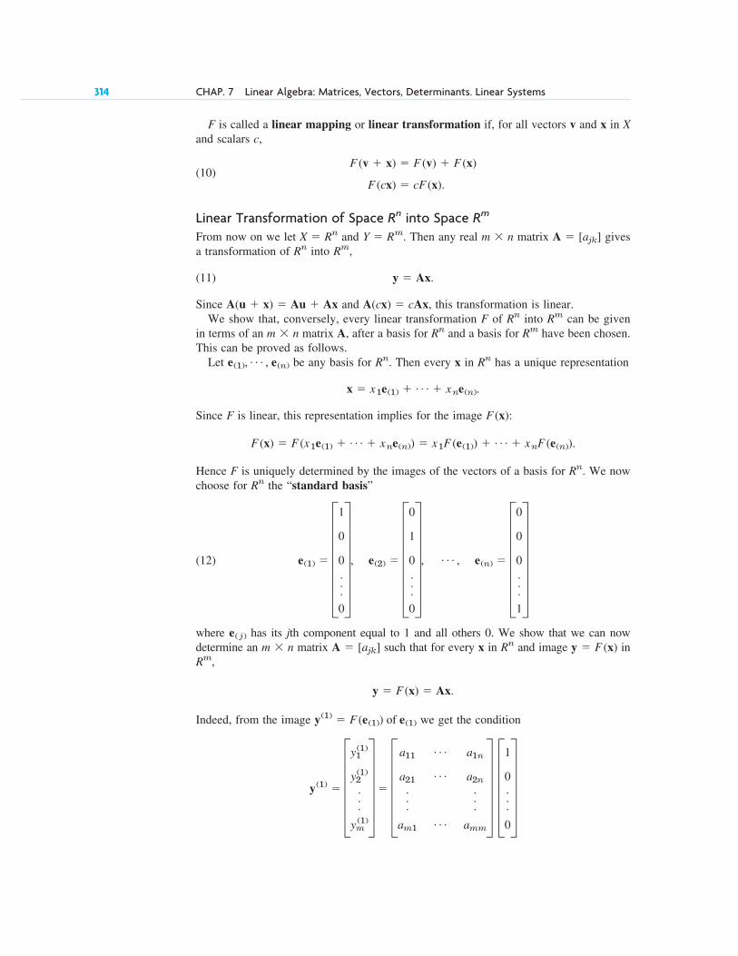
F is called a linear mapping or linear transformation if, for all vectors v and x in Xand scalars c,
(10)
Linear Transformation of Space into Space From now on we let and . Then any real matrix givesa transformation of into ,
(11) .
Since and , this transformation is linear.We show that, conversely, every linear transformation F of into can be given
in terms of an matrix A, after a basis for and a basis for have been chosen.This can be proved as follows.
Let be any basis for . Then every x in has a unique representation
.
Since F is linear, this representation implies for the image :
.
Hence F is uniquely determined by the images of the vectors of a basis for . We nowchoose for the “standard basis”
(12)
where has its jth component equal to 1 and all others 0. We show that we can nowdetermine an matrix such that for every x in and image in
,
.
Indeed, from the image we get the condition
y(1) � Fy1(1)
y2(1)
.
.
.
ym(1)
V � Fa11Á a1n
a21Á a2n
.
.
....
am1Á amm
V F10...
0
Vy(1) � F (e(1)) of e(1)
y � F (x) � Ax
Rmy � F (x)RnA � [ajk]m � n
e( j)
e(1) � G1
0
0
.
.
.
0
W, e(2) � G0
1
0
.
.
.
0
W, Á , e(n) � G0
0
0
.
.
.
1
WRn
Rn
F (x) � F (x1e(1) � Á � xne(n)) � x1F (e(1)) � Á � xnF (e(n))
F (x)
x � x1e(1) � Á � xne(n)
RnRne(1), Á , e(n)
RmRnm � nRmRn
A(cx) � cAxA(u � x) � Au � Ax
y � Ax
RmRnA � [ajk]m � nY � RmX � Rn
RmRn
F (cx) � cF (x).
F (v � x) � F (v) � F (x)
314 CHAP. 7 Linear Algebra: Matrices, Vectors, Determinants. Linear Systems

from which we can determine the first column of A, namely . Similarly, from the image of we get the second column of A, and so on.
This completes the proof.
We say that A represents F, or is a representation of F, with respect to the bases for and . Quite generally, the purpose of a “representation” is the replacement of oneobject of study by another object whose properties are more readily apparent.
In three-dimensional Euclidean space the standard basis is usually written . Thus,
(13) .
These are the three unit vectors in the positive directions of the axes of the Cartesiancoordinate system in space, that is, the usual coordinate system with the same scale ofmeasurement on the three mutually perpendicular coordinate axes.
E X A M P L E 5 Linear Transformations
Interpreted as transformations of Cartesian coordinates in the plane, the matrices
represent a reflection in the line , a reflection in the -axis, a reflection in the origin, and a stretch (when , or a contraction when ) in the -direction, respectively.
E X A M P L E 6 Linear Transformations
Our discussion preceding Example 5 is simpler than it may look at first sight. To see this, find A representingthe linear transformation that maps onto
Solution. Obviously, the transformation is
From this we can directly see that the matrix is
. Check: .
If A in (11) is square, , then (11) maps into . If this A is nonsingular, so thatexists (see Sec. 7.8), then multiplication of (11) by from the left and use of
gives the inverse transformation
(14) .
It maps every onto that x, which by (11) is mapped onto . The inverse of a lineartransformation is itself linear, because it is given by a matrix, as (14) shows.
y0y � y0
x � A�1y
A�1A � IA�1A�1
RnRnn � n
�c y1
y2
d � c2 �5
3 4d c x1
x2
d � c 2x1 � 5x2
3x1 � 4x2
dA � c2 �5
3 4d
y2 � 3x1 � 4x2.
y1 � 2x1 � 5x2
(2x1 � 5x2, 3x1 � 4x2).(x1, x2)
�x10 a 1a � 1x1x2 � x1
c0 1
1 0d , c1 0
0 �1d , c�1 0
0 �1d , ca 0
0 1d
i � D100
T , j � D010
T , k � D001
T
e(2) � j, e(3) � ke(1) � i,E 3
RmRn
�
e(2)am1 � ym(1)
Á ,a21 � y2(1),a11 � y1
(1),
SEC. 7.9 Vector Spaces, Inner Product Spaces, Linear Transformations Optional 315

Composition of Linear TransformationsWe want to give you a flavor of how linear transformations in general vector spaces work.You will notice, if you read carefully, that definitions and verifications (Example 7) strictlyfollow the given rules and you can think your way through the material by going in aslow systematic fashion.
The last operation we want to discuss is composition of linear transformations. Let X,Y, W be general vector spaces. As before, let F be a linear transformation from X to Y.Let G be a linear transformation from W to X. Then we denote, by H, the compositionof F and G, that is,
,
which means we take transformation G and then apply transformation F to it (in thatorder!, i.e. you go from left to right).
Now, to give this a more concrete meaning, if we let w be a vector in W, then is a vector in X and is a vector in Y. Thus, H maps W to Y, and we can write
(15)
which completes the definition of composition in a general vector space setting. But iscomposition really linear? To check this we have to verify that H, as defined in (15), obeysthe two equations of (10).
E X A M P L E 7 The Composition of Linear Transformations Is Linear
To show that H is indeed linear we must show that (10) holds. We have, for two vectors in W,
(by linearity of G)
(by linearity of F)
(by (15))
(by definition of H).
Similarly,
.
We defined composition as a linear transformation in a general vector space setting andshowed that the composition of linear transformations is indeed linear.
Next we want to relate composition of linear transformations to matrix multiplication.To do so we let and . This choice of particular vector spaces
allows us to represent the linear transformations as matrices and form matrix equations,as was done in (11). Thus F can be represented by a general real matrix and G by an matrix . Then we can write for F, with column vectors xwith n entries, and resulting vector y, with m entries
(16) y � Ax
B � 3bjk4n � pA � 3ajk4m � n
W � RpX � Rn, Y � Rm,
� � cF (G (w2)) � c (F � G)(w2) � cH(w2)
H (cw2) � (F � G)(cw2) � F (G (cw2)) � F (c (G (w2))
� H (w1) � H (w2)
� (F � G)(w1) � (F � G)(w2)
� F (G (w1)) � F (G (w2))
� F (G (w1) � G (w2))
� F (G (w1 � w2))
H (w1 � w2) � (F � G)(w1 � w2)
w1, w2
H (w) � (F � G) (w) � (FG) (w) � F(G(w)),
F (G (w))G (w)
H � F � G � FG � F(G)
316 CHAP. 7 Linear Algebra: Matrices, Vectors, Determinants. Linear Systems

and similarly for G, with column vector w with p entries,
(17)
Substituting (17) into (16) gives
(18) where .
This is (15) in a matrix setting, this is, we can define the composition of linear transfor-mations in the Euclidean spaces as multiplication by matrices. Hence, the real matrix C represents a linear transformation H which maps to with vector w, acolumn vector with p entries.
Remarks. Our discussion is similar to the one in Sec. 7.2, where we motivated the“unnatural” matrix multiplication of matrices. Look back and see that our current, moregeneral, discussion is written out there for the case of dimension and (You may want to write out our development by picking small distinct dimensions, suchas and , and writing down the matrices and vectors. This is a trickof the trade of mathematicians in that we like to develop and test theories on smallerexamples to see that they work.)
E X A M P L E 8 Linear Transformations. Composition
In Example 5 of Sec. 7.9, let A be the first matrix and B be the fourth matrix with . Then, applying B toa vector , stretches the element by a in the direction. Next, when we apply A to the“stretched” vector, we reflect the vector along the line , resulting in a vector . But thisrepresents, precisely, a geometric description for the composition H of two linear transformations F and Grepresented by matrices A and B. We now show that, for this example, our result can be obtained bystraightforward matrix multiplication, that is,
and as in (18) calculate
,
which is the same as before. This shows that indeed , and we see the composition of lineartransformations can be represented by a linear transformation. It also shows that the order of matrix multiplicationis important (!). You may want to try applying A first and then B, resulting in BA. What do you see? Does itmake geometric sense? Is it the same result as AB?
We have learned several abstract concepts such as vector space, inner product space,and linear transformation. The introduction of such concepts allows engineers andscientists to communicate in a concise and common language. For example, the conceptof a vector space encapsulated a lot of ideas in a very concise manner. For the student,learning such concepts provides a foundation for more advanced studies in engineering.
This concludes Chapter 7. The central theme was the Gaussian elimination of Sec. 7.3from which most of the other concepts and theory flowed. The next chapter again has acentral theme, that is, eigenvalue problems, an area very rich in applications such as inengineering, modern physics, and other areas.
�
AB � C
ABw � c0 1
a 0d cw1
w2
d � c w2
aw1
d
AB � c0 1
1 0d ca 0
0 1d � c0 1
a 0d
y � [w2 aw1]Tx1 � x2
x1w1w � [w1 w2]Ta � 1
p � 4m � 2, n � 3,
p � 2.n � 2,m � 2,
RnRpm � p
C � ABy � Ax � A(Bw) � (AB)w � ABw � Cw
x � Bw.
SEC. 7.9 Vector Spaces, Inner Product Spaces, Linear Transformations Optional 317

318 CHAP. 7 Linear Algebra: Matrices, Vectors, Determinants. Linear Systems
1. Basis. Find three bases of
2. Uniqueness. Show that the representation of any given vector in an n-dimensional
vector space V in terms of a given basis for V is unique. Hint. Take two representations andconsider the difference.
3–10 VECTOR SPACE
(More problems in Problem Set 9.4.) Is the given set, takenwith the usual addition and scalar multiplication, a vectorspace? Give reason. If your answer is yes, find the dimen-sion and a basis.
3. All vectors in satisfying
4. All skew-symmetric matrices.
5. All polynomials in x of degree 4 or less withnonnegative coefficients.
6. All functions with arbitraryconstants a and b.
7. All functions with any constant aand b.
8. All matrices A with fixed n and .
9. All matrices with .
10. All matrices with first column any multipleof
11–14 LINEAR TRANSFORMATIONS
Find the inverse transformation. Show the details.
11. 12. y1 � 3x1 � 2x2
y2 � 4x1 � x2
y1 � 0.5x1 � 0.5x2
y2 � 1.5x1 � 2.5x2
[3 0 �5]T.[ajk]3 � 2
a11 � a22 � 0[ajk]2 � 2
det A � 0n � n
y (x) � (ax � b)e�x
y (x) � a cos 2x � b sin 2x
3 � 3
�4v1 � v2 � v3 � 0.�v1 � 2v2 � 3v3 � 0,R3
a(1), Á , a(n)
� Á � cna(n)
v � c1a(1)
R2. 13.
14.
15–20 EUCLIDEAN NORMFind the Euclidean norm of the vectors:
15. 16.
17.
18. 19.
20.
21–25 INNER PRODUCT. ORTHOGONALITY21. Orthogonality. For what value(s) of k are the vectors
and orthogonal?
22. Orthogonality. Find all vectors in orthogonal toDo they form a vector space?
23. Triangle inequality. Verify (4) for the vectors inProbs. 15 and 18.
24. Cauchy–Schwarz inequality. Verify (3) for thevectors in Probs. 16 and 19.
25. Parallelogram equality. Verify (5) for the first twocolumn vectors of the coefficient matrix in Prob. 13.
32 0 14.R3
35 k 0 144
T32 12 �4 04T
312 �12 �
12
124
T
323 23
13 04T3�4 8 �14T
31 0 0 1 �1 0 �1 14T312
13 �
12 �
134
T33 1 �44T
y1 � 0.2x1 � 0.1x2
y2 � � 0.2x2 � 0.1x3
y3 � 0.1x1 � 0.1x3
y1 � 5x1 � 3x2 � 3x3
y2 � 3x1 � 2x2 � 2x3
y3 � 2x1 � x2 � 2x3
P R O B L E M S E T 7 . 9
1. What properties of matrix multiplication differ fromthose of the multiplication of numbers?
2. Let A be a matrix and B a matrix.Are the following expressions defined or not?
Givereasons.
3. Are there any linear systems without solutions? Withone solution? With more than one solution? Givesimple examples.
4. Let C be matrix and a a column vector with10 components. Are the following expressions definedor not? Ca, CTa, CaT, aC, aTC, (CaT)T.
10 � 10
A2, B2, AB, BA, AAT, BTA, BTB, BBT, BTAB. A � B,
100 � 50100 � 100
5. Motivate the definition of matrix multiplication.
6. Explain the use of matrices in linear transformations.
7. How can you give the rank of a matrix in terms of rowvectors? Of column vectors? Of determinants?
8. What is the role of rank in connection with solvinglinear systems?
9. What is the idea of Gauss elimination and backsubstitution?
10. What is the inverse of a matrix? When does it exist?How would you determine it?
C H A P T E R 7 R E V I E W Q U E S T I O N S A N D P R O B L E M S

11–20 MATRIX AND VECTOR CALCULATIONSShowing the details, calculate the following expressions orgive reason why they are not defined, when
11. AB, BA 12.
13. 14.
15. 16.
17.
18. 19.
20.
21–28 LINEAR SYSTEMS Showing the details, find all solutions or indicate that nosolution exists.
21.
22.
23.
24.
25.
26. 2x � 3y � 7z � 3
�4x � 6y � 14z � 7
0.3x � 0.7y � 1.3z � 3.24
0.9y � 0.8z � �2.53
0.7z � 1.19
�6x � 39y � 9z � �12
2x � 13y � 3z � 4
9x � 3y � 6z � 60
2x � 4y � 8z � 4
5x � 3y � z � 7
2x � 3y � z � 0
8x � 9y � 3z � 2
4y � z � 0
12x � 5y � 3z � 34
�6x � 4z � 8
(A � AT)(B � BT)
AB � BA(A2)�1, (A�1)2
det A, det A2, (det A)2, det B
A�1, B�1uTAu, vTBv
uTv, uvTAu, uTA
AT, BT
v � D 7
�3
3
Tu � D 2
0
�5
T ,
B � D 0 4 1
�4 0 �2
�1 2 0
T ,A � D 3 1 �3
1 4 2
�3 2 5
T ,
Chapter 7 Review Questions and Problems 319
27.
28.
29–32 RANKDetermine the ranks of the coefficient matrix and theaugmented matrix and state how many solutions the linearsystem will have.
29. In Prob. 23
30. In Prob. 24
31. In Prob. 27
32. In Prob. 26
33–35 NETWORKSFind the currents.
33.
34.
35.
10 V
130 V30 Ω
10 Ω
20 Ω
I2
I1
I3
10 Ω
5 Ω
20 Ω
I2
I1
I3
220 V
240 V
10 Ω
20 Ω
110 V
I1
I3
I2
�8x � 2z � 1
6y � 4z � 3
12x � 2y � 2
x � 2y � 6
3x � 5y � 20
�4x � y � �42

320 CHAP. 7 Linear Algebra: Matrices, Vectors, Determinants. Linear Systems
An matrix is a rectangular array of numbers or functions(“entries,” “elements”) arranged in m horizontal rows and n vertical columns. If
, the matrix is called square. A matrix is called a row vector and anmatrix a column vector (Sec. 7.1).
The sum of matrices of the same size (i.e., both is obtained byadding corresponding entries. The product of A by a scalar c is obtained bymultiplying each by c (Sec. 7.1).
The product of an matrix A by an matrix isdefined only when , and is the matrix with entries
(1)
This multiplication is motivated by the composition of linear transformations(Secs. 7.2, 7.9). It is associative, but is not commutative: if AB is defined, BA maynot be defined, but even if BA is defined, in general. Also maynot imply or or (Secs. 7.2, 7.8). Illustrations:
The transpose of a matrix is ; rows become columnsand conversely (Sec. 7.2). Here, A need not be square. If it is and , then Ais called symmetric; if , it is called skew-symmetric. For a product,
(Sec. 7.2).A main application of matrices concerns linear systems of equations
(2) (Sec. 7.3)
(m equations in n unknowns A and b given). The most important methodof solution is the Gauss elimination (Sec. 7.3), which reduces the system to“triangular” form by elementary row operations, which leave the set of solutionsunchanged. (Numeric aspects and variants, such as Doolittle’s and Cholesky’smethods, are discussed in Secs. 20.1 and 20.2.)
x1, Á , xn;
Ax � b
(AB)T � BTATA � �AT
A � ATAT � 3akj4A � 3ajk4AT
c34d [1 2] � c3 6
4 8d .[1 2] c3
4d � [11],
c�1 1
1 �1d c1 1
2 2d � c 1 1
�1 �1d
c1 1
2 2d c�1 1
1 �1d � c0 0
0 0d
BA � 0B � 0A � 0AB � 0AB � BA
(row j of A times
column k of B).cjk � aj1b1k � aj2b2k � Á � ajnbnk
C � 3cjk4m � pr � nB � [bjk]r � pm � nC � AB
ajk
m � n)A � Bm � 1
1 � nm � n
A � [ajk]m � n
SUMMARY OF CHAPTER 7Linear Algebra: Matrices, Vectors, Determinants. Linear Systems

Cramer’s rule (Secs. 7.6, 7.7) represents the unknowns in a system (2) of nequations in n unknowns as quotients of determinants; for numeric work it isimpractical. Determinants (Sec. 7.7) have decreased in importance, but will retaintheir place in eigenvalue problems, elementary geometry, etc.
The inverse of a square matrix satisfies . It exists if andonly if det A 0. It can be computed by the Gauss–Jordan elimination (Sec. 7.8).
The rank r of a matrix A is the maximum number of linearly independent rowsor columns of A or, equivalently, the number of rows of the largest square submatrixof A with nonzero determinant (Secs. 7.4, 7.7).
The system (2) has solutions if and only if rank , where is the augmented matrix (Fundamental Theorem, Sec. 7.5).
The homogeneous system
(3)
has solutions (“nontrivial solutions”) if and only if rank , in the caseequivalently if and only if (Secs. 7.6, 7.7).
Vector spaces, inner product spaces, and linear transformations are discussed inSec. 7.9. See also Sec. 7.4.
det A � 0m � nA nx � 0
Ax � 0
[A b]A � rank [A b]
�AA�1 � A�1A � IA�1
Summary of Chapter 7 321

322
C H A P T E R 8
Linear Algebra: Matrix Eigenvalue Problems
A matrix eigenvalue problem considers the vector equation
(1)
Here A is a given square matrix, an unknown scalar, and x an unknown vector. In amatrix eigenvalue problem, the task is to determine ’s and x’s that satisfy (1). Since
is always a solution for any and thus not interesting, we only admit solutionswith
The solutions to (1) are given the following names: The ’s that satisfy (1) are calledeigenvalues of A and the corresponding nonzero x’s that also satisfy (1) are calledeigenvectors of A.
From this rather innocent looking vector equation flows an amazing amount of relevanttheory and an incredible richness of applications. Indeed, eigenvalue problems come upall the time in engineering, physics, geometry, numerics, theoretical mathematics, biology,environmental science, urban planning, economics, psychology, and other areas. Thus, inyour career you are likely to encounter eigenvalue problems.
We start with a basic and thorough introduction to eigenvalue problems in Sec. 8.1 andexplain (1) with several simple matrices. This is followed by a section devoted entirelyto applications ranging from mass–spring systems of physics to population control modelsof environmental science. We show you these diverse examples to train your skills inmodeling and solving eigenvalue problems. Eigenvalue problems for real symmetric,skew-symmetric, and orthogonal matrices are discussed in Sec. 8.3 and their complexcounterparts (which are important in modern physics) in Sec. 8.5. In Sec. 8.4 we showhow by diagonalizing a matrix, we obtain its eigenvalues.
COMMENT. Numerics for eigenvalues (Secs. 20.6–20.9) can be studied immediatelyafter this chapter.
Prerequisite: Chap. 7.Sections that may be omitted in a shorter course: 8.4, 8.5.References and Answers to Problems: App. 1 Part B, App. 2.
l
x � 0.lx � 0
l
l
Ax � lx.

SEC. 8.1 The Matrix Eigenvalue Problem. Determining Eigenvalues and Eigenvectors 323
The following chart identifies where different types of eigenvalue problems appear in thebook.
Topic Where to find it
Matrix Eigenvalue Problem (algebraic eigenvalue problem) Chap. 8Eigenvalue Problems in Numerics Secs. 20.6–20.9Eigenvalue Problem for ODEs (Sturm–Liouville problems) Secs. 11.5, 11.6Eigenvalue Problems for Systems of ODEs Chap. 4Eigenvalue Problems for PDEs Secs. 12.3–12.11
8.1 The Matrix Eigenvalue Problem. DeterminingEigenvalues and Eigenvectors
Consider multiplying nonzero vectors by a given square matrix, such as
We want to see what influence the multiplication of the given matrix has on the vectors.In the first case, we get a totally new vector with a different direction and different lengthwhen compared to the original vector. This is what usually happens and is of no interesthere. In the second case something interesting happens. The multiplication produces avector which means the new vector has the same direction asthe original vector. The scale constant, which we denote by is 10. The problem ofsystematically finding such ’s and nonzero vectors for a given square matrix will be thetheme of this chapter. It is called the matrix eigenvalue problem or, more commonly, theeigenvalue problem.
We formalize our observation. Let be a given nonzero square matrix ofdimension Consider the following vector equation:
(1)
The problem of finding nonzero x’s and ’s that satisfy equation (1) is called an eigenvalueproblem.
Remark. So A is a given square matrix, x is an unknown vector, and is anunknown scalar. Our task is to find ’s and nonzero x’s that satisfy (1). Geometrically,we are looking for vectors, x, for which the multiplication by A has the same effect asthe multiplication by a scalar in other words, Ax should be proportional to x. Thus,the multiplication has the effect of producing, from the original vector x, a new vector
that has the same or opposite (minus sign) direction as the original vector. (This wasall demonstrated in our intuitive opening example. Can you see that the second equation inthat example satisfies (1) with and and A the given matrix?Write it out.) Now why do we require x to be nonzero? The reason is that isalways a solution of (1) for any value of because This is of no interest.A0 � 0.l,
x � 02 � 2x � [3 4]T,l � 10
lx
l;
l
l(!)
l
Ax � lx.
n � n.A � [ajk]
l
l
[30 40]T � 10 [3 4]T,
c6 3
4 7d c5
1d � c33
27d , c6 3
4 7d c3
4d � c30
40d .

324 CHAP. 8 Linear Algebra: Matrix Eigenvalue Problems
We introduce more terminology. A value of for which (1) has a solution iscalled an eigenvalue or characteristic value of the matrix A. Another term for is a latentroot. (“Eigen” is German and means “proper” or “characteristic.”). The correspondingsolutions of (1) are called the eigenvectors or characteristic vectors of Acorresponding to that eigenvalue . The set of all the eigenvalues of A is called thespectrum of A. We shall see that the spectrum consists of at least one eigenvalue and atmost of n numerically different eigenvalues. The largest of the absolute values of theeigenvalues of A is called the spectral radius of A, a name to be motivated later.
How to Find Eigenvalues and EigenvectorsNow, with the new terminology for (1), we can just say that the problem of determiningthe eigenvalues and eigenvectors of a matrix is called an eigenvalue problem. (However,more precisely, we are considering an algebraic eigenvalue problem, as opposed to aneigenvalue problem involving an ODE or PDE, as considered in Secs. 11.5 and 12.3, oran integral equation.)
Eigenvalues have a very large number of applications in diverse fields such as inengineering, geometry, physics, mathematics, biology, environmental science, economics,psychology, and other areas. You will encounter applications for elastic membranes,Markov processes, population models, and others in this chapter.
Since, from the viewpoint of engineering applications, eigenvalue problems are the mostimportant problems in connection with matrices, the student should carefully follow ourdiscussion.
Example 1 demonstrates how to systematically solve a simple eigenvalue problem.
E X A M P L E 1 Determination of Eigenvalues and Eigenvectors
We illustrate all the steps in terms of the matrix
Solution. (a) Eigenvalues. These must be determined first. Equation (1) is
Transferring the terms on the right to the left, we get
(2 )
This can be written in matrix notation
(3 )
because (1) is which gives (3 ). We see that this is a homogeneouslinear system. By Cramer’s theorem in Sec. 7.7 it has a nontrivial solution (an eigenvector of A we arelooking for) if and only if its coefficient determinant is zero, that is,
(4 ) D (l) � det (A � lI) � 2�5 � l 2
2 �2 � l2 � (�5 � l)(�2 � l) � 4 � l2 � 7l � 6 � 0.*
x � 0*Ax � lx � Ax � lIx � (A � lI)x � 0,
(A � lI)x � 0*
(�5 � l)x1 � 2x2 � 0
2x1 � (�2 � l)x2 � 0.*
Ax � c�5 2
2 �2d c x1
x2
d � l c x1
x2
d ; in components, �5x1 � 2x2 � lx1
2x1 � 2x2 � lx2.
A � c�5 2
2 �2d .
l
x � 0
l
x � 0,l,

We call the characteristic determinant or, if expanded, the characteristic polynomial, and the characteristic equation of A. The solutions of this quadratic equation are and . Theseare the eigenvalues of A.
( ) Eigenvector of A corresponding to . This vector is obtained from (2 ) with , that is,
A solution is , as we see from either of the two equations, so that we need only one of them. Thisdetermines an eigenvector corresponding to up to a scalar multiple. If we choose , we obtainthe eigenvector
( ) Eigenvector of A corresponding to . For , equation (2 ) becomes
A solution is with arbitrary . If we choose , we get Thus an eigenvector of Acorresponding to is
For the matrix in the intuitive opening example at the start of Sec. 8.1, the characteristic equation isThe eigenvalues are Corresponding eigenvectors are
and , respectively. The reader may want to verify this.
This example illustrates the general case as follows. Equation (1) written in components is
Transferring the terms on the right side to the left side, we have
(2)
In matrix notation,
(3) (A � lI)x � 0.
(a11 � l)x1 � a12x2 � Á � a1nxn � 0
a21x1 � (a22 � l)x2 � Á � a2nxn � 0
. . . . . . . . . . . . . . . . . . . . . . . . . . . . . . . . . . . . . . . . . . . . . .
an1x1 � an2x2 � Á � (ann � l)xn � 0.
a11x1 � Á � a1nxn � lx1
a21x1 � Á � a2nxn � lx2
# # # # # # # # # # # # # # # # # # # # # # #
an1x1 � Á � annxn � lxn.
�[�1 1]T[3 4]T{10, 3}.l2 � 13l � 30 � (l � 10)(l � 3) � 0.
x2 � c 2
�1d , Check: Ax2 � c�5 2
2 �2d c 2
�1d � c�12
6d � (�6)x2 � l2x2.
l2 � �6x2 � �1.x1 � 2x1x2 � �x1>2
2x1 � 4x2 � 0.
x1 � 2x2 � 0
*l � l2 � �6l2b2
x1 � c12d , Check: Ax1 � c�5 2
2 �2d c1
2d � c�1
�2d � (�1)x1 � l1x1.
x1 � 1l1 � �1x2 � 2x1
2x1 � x2 � 0.
�4x1 � 2x2 � 0
l � l1 � �1*l1b1
l2 � �6l1 � �1D (l) � 0D (l)
SEC. 8.1 The Matrix Eigenvalue Problem. Determining Eigenvalues and Eigenvectors 325

326 CHAP. 8 Linear Algebra: Matrix Eigenvalue Problems
By Cramer’s theorem in Sec. 7.7, this homogeneous linear system of equations has anontrivial solution if and only if the corresponding determinant of the coefficients is zero:
(4)
is called the characteristic matrix and the characteristic determinant ofA. Equation (4) is called the characteristic equation of A. By developing we obtaina polynomial of nth degree in . This is called the characteristic polynomial of A.
This proves the following important theorem.
T H E O R E M 1 Eigenvalues
The eigenvalues of a square matrix A are the roots of the characteristic equation(4) of A.
Hence an n � n matrix has at least one eigenvalue and at most n numericallydifferent eigenvalues.
For larger n, the actual computation of eigenvalues will, in general, require the use of Newton’s method (Sec. 19.2) or another numeric approximation method in Secs.20.7–20.9.
The eigenvalues must be determined first. Once these are known, correspondingeigenvectors are obtained from the system (2), for instance, by the Gauss elimination,where is the eigenvalue for which an eigenvector is wanted. This is what we did inExample 1 and shall do again in the examples below. (To prevent misunderstandings:numeric approximation methods, such as in Sec. 20.8, may determine eigenvectors first.)
Eigenvectors have the following properties.
T H E O R E M 2 Eigenvectors, Eigenspace
If w and x are eigenvectors of a matrix A corresponding to the same eigenvalueso are (provided ) and kx for any .
Hence the eigenvectors corresponding to one and the same eigenvalue of A,together with 0, form a vector space (cf. Sec. 7.4), called the eigenspace of Acorresponding to that .
P R O O F and imply and hence
In particular, an eigenvector x is determined only up to a constant factor. Hence wecan normalize x, that is, multiply it by a scalar to get a unit vector (see Sec. 7.9). For instance, in Example 1 has the length hence
is a normalized eigenvector (a unit eigenvector).[1>15 2>15]T�x1� � 212 � 22 � 15;x1 � [1 2]T
�A (kw � /x) � l (kw � /x).A (kw) � k (Aw) � k (lw) � l (kw);A(w � x) � Aw � Ax � lw � lx � l(w � x)Ax � lxAw � lw
l
l
k � 0x � �ww � xl,
l
l
D(l)D (l)A � lI
D(l) � det (A � lI) � 5a11 � l a12Á a1n
a21 a22 � l Á a2n
# # Á #
an1 an2Á ann � l
5 � 0.

Examples 2 and 3 will illustrate that an matrix may have n linearly independenteigenvectors, or it may have fewer than n. In Example 4 we shall see that a real matrixmay have complex eigenvalues and eigenvectors.
E X A M P L E 2 Multiple Eigenvalues
Find the eigenvalues and eigenvectors of
Solution. For our matrix, the characteristic determinant gives the characteristic equation
The roots (eigenvalues of A) are (If you have trouble finding roots, you may want touse a root finding algorithm such as Newton’s method (Sec. 19.2). Your CAS or scientific calculator can findroots. However, to really learn and remember this material, you have to do some exercises with paper and pencil.)To find eigenvectors, we apply the Gauss elimination (Sec. 7.3) to the system , first with and then with . For the characteristic matrix is
Hence it has rank 2. Choosing we have from and then fromHence an eigenvector of A corresponding to is .
For the characteristic matrix
Hence it has rank 1. From we have Choosing and, we obtain two linearly independent eigenvectors of A corresponding to [as they must
exist by (5), Sec. 7.5, with and
and
The order of an eigenvalue as a root of the characteristic polynomial is called thealgebraic multiplicity of The number of linearly independent eigenvectorscorresponding to is called the geometric multiplicity of Thus is the dimensionof the eigenspace corresponding to this l.
mll.l
mll.lMl
�x3 � D301
T .
x2 � D�2
1
0
Tn � 3],rank � 1
l � �3x2 � 0, x3 � 1x2 � 1, x3 � 0x1 � �2x2 � 3x3.x1 � 2x2 � 3x3 � 0
A � lI � A � 3I � D 1 2 �3
2 4 �6
�1 �2 3
T row-reduces to D1 2 �3
0 0 0
0 0 0
T .l � �3
x1 � [1 2 �1]Tl � 5�7x1 � 2x2 � 3x3 � 0.x1 � 1�
247 x2 � 48
7 x3 � 0x2 � 2x3 � �1
A � lI � A � 5I � D�7 2 �3
2 �4 �6
�1 �2 �5
T . It row-reduces to D�7 2 �3
0 � 247 �
487
0 0 0
T .l � 5l � �3
l � 5(A � lI)x � 0
l1 � 5, l2 � l3 � �3.
�l3 � l2 � 21l � 45 � 0.
A � D�2 2 �3
2 1 �6
�1 �2 0
T .
n � n
SEC. 8.1 The Matrix Eigenvalue Problem. Determining Eigenvalues and Eigenvectors 327

328 CHAP. 8 Linear Algebra: Matrix Eigenvalue Problems
Since the characteristic polynomial has degree n, the sum of all the algebraicmultiplicities must equal n. In Example 2 for we have In general,
, as can be shown. The difference is called the defect of Thus in Example 2, but positive defects can easily occur:
E X A M P L E 3 Algebraic Multiplicity, Geometric Multiplicity. Positive Defect
The characteristic equation of the matrix
Hence is an eigenvalue of algebraic multiplicity . But its geometric multiplicity is only since eigenvectors result from , hence , in the form . Hence for the defectis
Similarly, the characteristic equation of the matrix
Hence is an eigenvalue of algebraic multiplicity , but its geometric multiplicity is only since eigenvectors result from in the form
E X A M P L E 4 Real Matrices with Complex Eigenvalues and Eigenvectors
Since real polynomials may have complex roots (which then occur in conjugate pairs), a real matrix may havecomplex eigenvalues and eigenvectors. For instance, the characteristic equation of the skew-symmetric matrix
It gives the eigenvalues . Eigenvectors are obtained from and, respectively, and we can choose to get
In the next section we shall need the following simple theorem.
T H E O R E M 3 Eigenvalues of the Transpose
The transpose AT of a square matrix A has the same eigenvalues as A.
P R O O F Transposition does not change the value of the characteristic determinant, as follows fromTheorem 2d in Sec. 7.7. �
Having gained a first impression of matrix eigenvalue problems, we shall illustrate theirimportance with some typical applications in Sec. 8.2.
�c1id and c 1
�id .
x1 � 1ix1 � x2 � 0�ix1 � x2 � 0l1 � i (� 1�1), l2 � �i
A � c 0 1
�1 0d is det (A � lI) � 2 �l 1
�1 �l 2 � l2 � 1 � 0.
�[x1 0]T.0x1 � 2x2 � 0m3 � 1,M3 � 2l � 3
A � c3 2
0 3d is det (A � lI) � 2 3 � l 2
0 3 � l 2 � (3 � l)2 � 0.
¢0 � 1.l � 0[x1 0]Tx2 � 0�0x1 � x2 � 0
m0 � 1,M0 � 2l � 0
A � c0 1
0 0d is det (A � lI) � 2 �l 1
0 �l 2 � l2 � 0.
¢l¢�3 � 0l.¢l � Ml � mlml � Ml
ml � Ml � 2.l � �3

SEC. 8.2 Some Applications of Eigenvalue Problems 329
1–16 EIGENVALUES, EIGENVECTORSFind the eigenvalues. Find the corresponding eigenvectors.Use the given or factor in Probs. 11 and 15.
1. 2.
3. 4.
5. 6.
7. 8.
9. 10.
11.
12. 13.
14. D2 0 �1
0 12 0
1 0 4
TD13 5 2
2 7 �8
5 4 7
TD3 5 3
0 4 6
0 0 1
TD 6 2 �2
2 5 0
�2 0 7
T , l � 3
c cos u �sin u
sin u cos udc 0.8 �0.6
0.6 0.8d
c a b
�b adc0 1
0 0d
c1 2
0 3dc 0 3
�3 0d
c 1 2
2 4dc5 �2
9 �6d
c0 0
0 0dc3.0 0
0 �0.6d
l 15.
16.
17–20 LINEAR TRANSFORMATIONS AND EIGENVALUES
Find the matrix A in the linear transformation where ( ) are Cartesiancoordinates. Find the eigenvalues and eigenvectors andexplain their geometric meaning.
17. Counterclockwise rotation through the angle aboutthe origin in .
18. Reflection about the -axis in
19. Orthogonal projection (perpendicular projection) of onto the -axis.
20. Orthogonal projection of onto the plane
21–25 GENERAL PROBLEMS
21. Nonzero defect. Find further and matrices with positive defect. See Example 3.
22. Multiple eigenvalues. Find further and matrices with multiple eigenvalues. See Example 2.
23. Complex eigenvalues. Show that the eigenvalues of areal matrix are real or complex conjugate in pairs.
24. Inverse matrix. Show that exists if and only ifthe eigenvalues are all nonzero, and then
has the eigenvalues
25. Transpose. Illustrate Theorem 3 with examples of yourown.
1>l1, Á , 1>ln.A�1l1, Á , ln
A�1
3 � 32 � 2
3 � 32 � 2
x2 � x1.R3
x2
R2
R2.x1
R2p>2
x � [x1 x2 x3]Tx � [x1 x2]Ty � Ax,
E�3 0 4 2
0 1 �2 4
2 4 �1 �2
0 2 �2 3
UE�1 0 12 0
0 �1 0 12
0 0 �1 �4
0 0 �4 �1
U, (l � 1)2
P R O B L E M S E T 8 . 1
8.2 Some Applications of Eigenvalue ProblemsWe have selected some typical examples from the wide range of applications of matrixeigenvalue problems. The last example, that is, Example 4, shows an application involvingvibrating springs and ODEs. It falls into the domain of Chapter 4, which covers matrixeigenvalue problems related to ODE’s modeling mechanical systems and electrical

networks. Example 4 is included to keep our discussion independent of Chapter 4.(However, the reader not interested in ODEs may want to skip Example 4 without lossof continuity.)
E X A M P L E 1 Stretching of an Elastic Membrane
An elastic membrane in the -plane with boundary circle (Fig. 160) is stretched so that a pointP: goes over into the point Q: given by
(1)
Find the principal directions, that is, the directions of the position vector x of P for which the direction of theposition vector y of Q is the same or exactly opposite. What shape does the boundary circle take under thisdeformation?
Solution. We are looking for vectors x such that . Since , this gives , the equationof an eigenvalue problem. In components, is
(2) or
The characteristic equation is
(3)
Its solutions are and These are the eigenvalues of our problem. For our system (2)becomes
For , our system (2) becomes
We thus obtain as eigenvectors of A, for instance, corresponding to and corresponding to(or a nonzero scalar multiple of these). These vectors make and angles with the positive x1-direction.
They give the principal directions, the answer to our problem. The eigenvalues show that in the principaldirections the membrane is stretched by factors 8 and 2, respectively; see Fig. 160.
Accordingly, if we choose the principal directions as directions of a new Cartesian -coordinate system,say, with the positive -semi-axis in the first quadrant and the positive -semi-axis in the second quadrant ofthe -system, and if we set then a boundary point of the unstretched circularmembrane has coordinates Hence, after the stretch we have
Since , this shows that the deformed boundary is an ellipse (Fig. 160)
(4) �z1
2
82 �
z22
22 � 1.
cos2 � � sin2 � � 1
z1 � 8 cos �, z2 � 2 sin �.
cos �, sin �.u1 � r cos �, u2 � r sin �,x1x2
u2u1
u1u2
135°45°l2
[1 �1]Tl1[1 1]T
3x1 � 3x2 � 0,
3x1 � 3x2 � 0. 2 Solution x2 � �x1, x1 arbitrary,
for instance, x1 � 1, x2 � �1.
l2 � 2
�3x1 � 3x2 � 0,
3x1 � 3x2 � 0. 2 Solution x2 � x1, x1 arbitrary,
for instance, x1 � x2 � 1.
l � l1 � 8,l2 � 2.l1 � 8
2 5 � l 3
3 5 � l 2 � (5 � l)2 � 9 � 0.
(5 � l)x1 � 3x2 � 0
3x1 � (5 � l)x2 � 0.
5x1 � 3x2 � lx1
3x1 � 5x2 � lx2
Ax � lxAx � lxy � Axy � lx
y � c y1
y2
d � Ax � c5 3
3 5d c x1
x2
d ; in components, y1 � 5x1 � 3x2
y2 � 3x1 � 5x2.
(y1, y2)(x1, x2)x1
2 � x22 � 1x1x2
330 CHAP. 8 Linear Algebra: Matrix Eigenvalue Problems

SEC. 8.2 Some Applications of Eigenvalue Problems 331
Fig. 160. Undeformed and deformed membrane in Example 1
x1
x2
Principal
directionPr
incipa
l
direc
tion
E X A M P L E 2 Eigenvalue Problems Arising from Markov Processes
Markov processes as considered in Example 13 of Sec. 7.2 lead to eigenvalue problems if we ask for the limitstate of the process in which the state vector x is reproduced under the multiplication by the stochastic matrixA governing the process, that is, . Hence A should have the eigenvalue 1, and x should be a correspondingeigenvector. This is of practical interest because it shows the long-term tendency of the development modeledby the process.
In that example,
Hence has the eigenvalue 1, and the same is true for A by Theorem 3 in Sec. 8.1. An eigenvector x of Afor is obtained from
Taking , we get from and then from Thisgives It means that in the long run, the ratio Commercial:Industrial:Residential will approach2:6:1, provided that the probabilities given by A remain (about) the same. (We switched to ordinary fractionsto avoid rounding errors.)
E X A M P L E 3 Eigenvalue Problems Arising from Population Models. Leslie Model
The Leslie model describes age-specified population growth, as follows. Let the oldest age attained by thefemales in some animal population be 9 years. Divide the population into three age classes of 3 years each. Letthe “Leslie matrix” be
(5)
where is the average number of daughters born to a single female during the time she is in age class k, andis the fraction of females in age class that will survive and pass into class j. (a) What is the
number of females in each class after 3, 6, 9 years if each class initially consists of 400 females? (b) For what initialdistribution will the number of females in each class change by the same proportion? What is this rate of change?
j � 1lj, j�1( j � 2, 3)l1k
L � [ljk] � D0 2.3 0.4
0.6 0 0
0 0.3 0
T
�
x � [2 6 1]T.�3x1>10 � x2>10 � 0.x1 � 2�x2>30 � x3>5 � 0x2 � 6x3 � 1
A � I � D�0.3 0.1 0
0.2 �0.1 0.2
0.1 0 �0.2
T , row-reduced to D� 310
110 0
0 � 130
15
0 0 0
T .l � 1
AT
A � D0.7 0.1 0
0.2 0.9 0.2
0.1 0 0.8
T . For the transpose, D0.7 0.2 0.1
0.1 0.9 0
0 0.2 0.8
T D111
T � D111
T .
Ax � x

332 CHAP. 8 Linear Algebra: Matrix Eigenvalue Problems
Solution. (a) Initially, After 3 years,
Similarly, after 6 years the number of females in each class is given by andafter 9 years we have
(b) Proportional change means that we are looking for a distribution vector x such that , where isthe rate of change (growth if decrease if ). The characteristic equation is (develop the characteristicdeterminant by the first column)
A positive root is found to be (for instance, by Newton’s method, Sec. 19.2) A corresponding eigenvectorx can be determined from the characteristic matrix
where is chosen, then follows from and fromTo get an initial population of 1200 as before, we multiply x byAnswer: Proportional growth of the numbers of females in the three classes
will occur if the initial values are 738, 369, 92 in classes 1, 2, 3, respectively. The growth rate will be 1.2 per3 years.
E X A M P L E 4 Vibrating System of Two Masses on Two Springs (Fig. 161)
Mass–spring systems involving several masses and springs can be treated as eigenvalue problems. For instance,the mechanical system in Fig. 161 is governed by the system of ODEs
(6)
where and are the displacements of the masses from rest, as shown in the figure, and primes denotederivatives with respect to time t. In vector form, this becomes
(7)
Fig. 161. Masses on springs in Example 4
k1
= 3
k2
= 2 (Net change in spring length = y
2 – y
1)
System inmotion
System instatic
equilibrium
m1
= 1(y1
= 0)
(y2
= 0) m2
= 1
y1
y2
y2
y1
ys � c y1s
y2sd � Ay � c�5 2
2 �2d c y1
y2
d .
y2y1
y1s � �3y1 � 2(y1 � y2) � �5y1 � 2y2
y2s � �2(y2 � y1) � 2y1 � 2y2
�
1200>(1 � 0.5 � 0.125) � 738.�1.2x1 � 2.3x2 � 0.4x3 � 0.
x1 � 10.3x2 � 1.2x3 � 0,x2 � 0.5x3 � 0.125
A � 1.2I � D�1.2 2.3 0.4
0.6 �1.2 0
0 0.3 �1.2
T , say, x � D 1
0.5
0.125
Tl � 1.2.
det (L � lI) � �l3 � 0.6(�2.3l � 0.3 # 0.4) � �l3 � 1.38l � 0.072 � 0.
l 1l � 1,lLx � lx
x(9)T � (Lx(6))
T � [1519.2 360 194.4].x(6)
T � (Lx(3))T � [600 648 72],
x(3) � Lx(0) � D0 2.3 0.4
0.6 0 0
0 0.3 0
T D400
400
400
T � D1080
240
120
T .x(0)
T � [400 400 400].

SEC. 8.2 Some Applications of Eigenvalue Problems 333
1–6 ELASTIC DEFORMATIONSGiven A in a deformation find the principaldirections and corresponding factors of extension orcontraction. Show the details.
1. 2.
3. 4.
5. 6. c1.25 0.75
0.75 1.25dc1 1
2
12 1
dc5 2
2 13dc 7 16
16 2d
c 2.0 0.4
0.4 2.0dc3.0 1.5
1.5 3.0d
y � Ax,
7–9 MARKOV PROCESSESFind the limit state of the Markov process modeled by thegiven matrix. Show the details.
7.
8. 9. D0.6 0.1 0.2
0.4 0.1 0.4
0 0.8 0.4
TD0.4 0.3 0.3
0.3 0.6 0.1
0.3 0.1 0.6
Tc0.2 0.5
0.8 0.5d
P R O B L E M S E T 8 . 2
We try a vector solution of the form
(8)
This is suggested by a mechanical system of a single mass on a spring (Sec. 2.4), whose motion is given byexponential functions (and sines and cosines). Substitution into (7) gives
Dividing by and writing we see that our mechanical system leads to the eigenvalue problem
(9) where
From Example 1 in Sec. 8.1 we see that A has the eigenvalues and Consequently,and respectively. Corresponding eigenvectors are
(10)
From (8) we thus obtain the four complex solutions [see (10), Sec. 2.2]
By addition and subtraction (see Sec. 2.2) we get the four real solutions
A general solution is obtained by taking a linear combination of these,
with arbitrary constants (to which values can be assigned by prescribing initial displacement andinitial velocity of each of the two masses). By (10), the components of y are
These functions describe harmonic oscillations of the two masses. Physically, this had to be expected becausewe have neglected damping. �
y2 � 2a1 cos t � 2b1 sin t � a2 cos 16 t � b2 sin 16 t.
y1 � a1 cos t � b1 sin t � 2a2 cos 16 t � 2b2 sin 16 t
a1, b1, a2, b2
y � x1 (a1 cos t � b1 sin t) � x2 (a2 cos 16 t � b2 sin 16 t)
x1 cos t, x1 sin t, x2 cos 16 t, x2 sin 16 t.
x2e�i26t � x2 (cos 16 t � i sin 16 t).
x1e�it � x1 (cos t � i sin t),
x1 � c12d and x2 � c 2
�1d .
1�6 � �i16,v � �1�1 � �il2 � �6.l1 � �1
l � v2.Ax � lx
v2 � l,evt
v2xevt � Axevt.
y � xevt.

334 CHAP. 8 Linear Algebra: Matrix Eigenvalue Problems
1WASSILY LEONTIEF (1906–1999). American economist at New York University. For his input–outputanalysis he was awarded the Nobel Prize in 1973.
10–12 AGE-SPECIFIC POPULATIONFind the growth rate in the Leslie model (see Example 3)with the matrix as given. Show the details.
10. 11.
12.
13–15 LEONTIEF MODELS1
13. Leontief input–output model. Suppose that threeindustries are interrelated so that their outputs are usedas inputs by themselves, according to the consumption matrix
where is the fraction of the output of industry kconsumed (purchased) by industry j. Let be the pricecharged by industry j for its total output. A problem isto find prices so that for each industry, totalexpenditures equal total income. Show that this leadsto , where , and find asolution p with nonnegative
14. Show that a consumption matrix as considered in Prob.13 must have column sums 1 and always has theeigenvalue 1.
15. Open Leontief input–output model. If not the wholeoutput but only a portion of it is consumed by the
p1, p2, p3.p � [p1 p2 p3]TAp � p
pj
ajk
A � [ajk] � D0.1 0.5 0
0.8 0 0.4
0.1 0.5 0.6
T3 � 3
E0 3.0 2.0 2.0
0.5 0 0 0
0 0.5 0 0
0 0 0.1 0
UD0 3.45 0.60
0.90 0 0
0 0.45 0
TD0 9.0 5.0
0.4 0 0
0 0.4 0
Tindustries themselves, then instead of (as in Prob.13), we have , where is produced, Ax is consumed by the industries, and, thus,y is the net production available for other consumers.Find for what production x a given demand vector
can be achieved if the consump-tion matrix is
16–20 GENERAL PROPERTIES OF EIGENVALUEPROBLEMS
Let be an matrix with (not necessarilydistinct) eigenvalues Show.
16. Trace. The sum of the main diagonal entries, calledthe trace of A, equals the sum of the eigenvalues of A.
17. “Spectral shift.” has the eigenvaluesand the same eigenvectors as A.
18. Scalar multiples, powers. kA has the eigenvalueshas the eigenvalues
. The eigenvectors are those of A.
19. Spectral mapping theorem. The “polynomialmatrix”
has the eigenvalues
where , and the same eigenvectors as A.
20. Perron’s theorem. A Leslie matrix L with positivehas a positive eigenvalue. (This is a
special case of the Perron–Frobenius theorem in Sec.20.7, which is difficult to prove in its general form.)
l12, l13, l21, l32
j � 1, Á , n
p (lj) � kmljm � km�1lj
m�1 � Á � k1lj � k0
p (A) � kmAm � km�1Am�1 � Á � k1A � k0I
l1m, Á , ln
mkl1, Á , kln. Am(m � 1, 2, Á )
l1 � k, Á , ln � kA � kI
l1, Á , ln.n � nA � [ajk]
A � D0.1 0.4 0.2
0.5 0 0.1
0.1 0.4 0.4
T .y � [0.1 0.3 0.1]T
x � [x1 x2 x3]Tx � Ax � yAx � x
8.3 Symmetric, Skew-Symmetric, and Orthogonal Matrices
We consider three classes of real square matrices that, because of their remarkableproperties, occur quite frequently in applications. The first two matrices have already beenmentioned in Sec. 7.2. The goal of Sec. 8.3 is to show their remarkable properties.

SEC. 8.3 Symmetric, Skew-Symmetric, and Orthogonal Matrices 335
D E F I N I T I O N S Symmetric, Skew-Symmetric, and Orthogonal Matrices
A real square matrix is calledsymmetric if transposition leaves it unchanged,
(1) thus
skew-symmetric if transposition gives the negative of A,
(2) , thus
orthogonal if transposition gives the inverse of A,
(3)
E X A M P L E 1 Symmetric, Skew-Symmetric, and Orthogonal Matrices
The matrices
are symmetric, skew-symmetric, and orthogonal, respectively, as you should verify. Every skew-symmetricmatrix has all main diagonal entries zero. (Can you prove this?)
Any real square matrix A may be written as the sum of a symmetric matrix R and a skew-symmetric matrix S, where
(4) and
E X A M P L E 2 Illustration of Formula (4)
T H E O R E M 1 Eigenvalues of Symmetric and Skew-Symmetric Matrices
(a) The eigenvalues of a symmetric matrix are real.
(b) The eigenvalues of a skew-symmetric matrix are pure imaginary or zero.
This basic theorem (and an extension of it) will be proved in Sec. 8.5.
�A � D9 5 2
2 3 �8
5 4 3
T � R � S � D9.0 3.5 3.5
3.5 3.0 �2.0
3.5 �2.0 3.0
T � D 0 1.5 �1.5
�1.5 0 �6.0
1.5 6.0 0
T
S � 12 (A � AT).R � 1
2 (A � AT)
�
D�3 1 5
1 0 �2
5 �2 4
T , D 0 9 �12
�9 0 20
12 �20 0
T , D 23
13
23
�23
23
13
13
23 �2
3
T
AT � A�1.
akj � �ajk,AT � �A
akj � ajk,AT � A,
A � [ajk]

E X A M P L E 3 Eigenvalues of Symmetric and Skew-Symmetric Matrices
The matrices in (1) and (7) of Sec. 8.2 are symmetric and have real eigenvalues. The skew-symmetric matrixin Example 1 has the eigenvalues 0, �25 i, and 25 i. (Verify this.) The following matrix has the real eigenvalues1 and 5 but is not symmetric. Does this contradict Theorem 1?
Orthogonal Transformations and Orthogonal MatricesOrthogonal transformations are transformations
(5) where A is an orthogonal matrix.
With each vector x in such a transformation assigns a vector y in . For instance,the plane rotation through an angle
(6)
is an orthogonal transformation. It can be shown that any orthogonal transformation inthe plane or in three-dimensional space is a rotation (possibly combined with a reflectionin a straight line or a plane, respectively).
The main reason for the importance of orthogonal matrices is as follows.
T H E O R E M 2 Invariance of Inner Product
An orthogonal transformation preserves the value of the inner product of vectorsa and b in , defined by
(7)
That is, for any a and b in , orthogonal matrix A, and we have
Hence the transformation also preserves the length or norm of any vector a ingiven by
(8)
P R O O F Let A be orthogonal. Let and . We must show that Nowby (10d) in Sec. 7.2 and by (3). Hence
(9)
From this the invariance of follows if we set �b � a.� a �
u • v � uTv � (Aa)TAb � aTATAb � aTIb � aTb � a • b.
ATA � A�1A � I(Aa)T � aTATu • v � a • b.v � Abu � Aa
� a � � 1a • a � 2aTa.
Rn
u • v � a • b.u � Aa, v � Abn � nRn
a • b � aTb � [a1 Á
an] Db1
.
.
.
bn
T .Rn
y � c y1
y2
d � c cos u �sin u
sin u cos ud c x1
x2
du
RnRn
y � Ax
�c3 4
1 3d
336 CHAP. 8 Linear Algebra: Matrix Eigenvalue Problems

SEC. 8.3 Symmetric, Skew-Symmetric, and Orthogonal Matrices 337
Orthogonal matrices have further interesting properties as follows.
T H E O R E M 3 Orthonormality of Column and Row Vectors
A real square matrix is orthogonal if and only if its column vectors (andalso its row vectors) form an orthonormal system, that is,
(10)
P R O O F (a) Let A be orthogonal. Then . In terms of column vectors
(11)
The last equality implies (10), by the definition of the unit matrix I. From (3) itfollows that the inverse of an orthogonal matrix is orthogonal (see CAS Experiment 12).Now the column vectors of are the row vectors of A. Hence the row vectorsof A also form an orthonormal system.(b) Conversely, if the column vectors of A satisfy (10), the off-diagonal entries in (11)must be 0 and the diagonal entries 1. Hence , as (11) shows. Similarly, This implies because also and the inverse is unique. HenceA is orthogonal. Similarly when the row vectors of A form an orthonormal system, bywhat has been said at the end of part (a).
T H E O R E M 4 Determinant of an Orthogonal Matrix
The determinant of an orthogonal matrix has the value or
P R O O F From (Sec. 7.8, Theorem 4) and (Sec. 7.7,Theorem 2d), we get for an orthogonal matrix
E X A M P L E 4 Illustration of Theorems 3 and 4
The last matrix in Example 1 and the matrix in (6) illustrate Theorems 3 and 4 because their determinants are and , as you should verify.
T H E O R E M 5 Eigenvalues of an Orthogonal Matrix
The eigenvalues of an orthogonal matrix A are real or complex conjugates in pairsand have absolute value 1.
��1�1
�1 � det I � det (AA�1) � det (AAT) � det A det AT � (det A)2.
det AT � det Adet AB � det A det B
�1.�1
�
A�1A � AA�1 � IAT � A�1AAT � I.ATA � I
A�1(�AT)
n � n
I � A�1A � ATA � Da1T
.
.
.
anT
T [a1Á an] � Da1
Ta1 a1Ta2 � �� a1
Tan
� � � � � �
anTa1 an
Ta2 � �� anTan
T .a1, Á , an,A�1A � ATA � I
aj • ak � ajTak � e 0 if j � k
1 if j � k.
a1, Á , an

P R O O F The first part of the statement holds for any real matrix A because its characteristicpolynomial has real coefficients, so that its zeros (the eigenvalues of A) must be as indicated. The claim that will be proved in Sec. 8.5.
E X A M P L E 5 Eigenvalues of an Orthogonal Matrix
The orthogonal matrix in Example 1 has the characteristic equation
Now one of the eigenvalues must be real (why?), hence or . Trying, we find . Division by gives and the two eigenvalues and , which have absolutevalue 1. Verify all of this.
Looking back at this section, you will find that the numerous basic results it contains haverelatively short, straightforward proofs. This is typical of large portions of matrixeigenvalue theory.
�(5 � i111)>6(5 � i111)>6�(l2 � 5l>3 � 1) � 0
l � 1�1�1�1
�l3 � 23 l2 � 2
3 l � 1 � 0.
�ƒl ƒ � 1
338 CHAP. 8 Linear Algebra: Matrix Eigenvalue Problems
1–10 SPECTRUMAre the following matrices symmetric, skew-symmetric, ororthogonal? Find the spectrum of each, thereby illustratingTheorems 1 and 5. Show your work in detail.
1. 2.
3. 4.
5. 6.
7. 8.
9. 10.
11. WRITING PROJECT. Section Summary. Sum-marize the main concepts and facts in this section,giving illustrative examples of your own.
12. CAS EXPERIMENT. Orthogonal Matrices.
(a) Products. Inverse. Prove that the product of twoorthogonal matrices is orthogonal, and so is the inverseof an orthogonal matrix. What does this mean in termsof rotations?
D 49
89
19
�79
49 �4
9
�49
19
89
TD 0 0 1
0 1 0
�1 0 0
TD1 0 0
0 cos u �sin u
0 sin u cos u
TD 0 9 �12
�9 0 20
12 �20 0
TDa k k
k a k
k k a
TD6 0 0
0 2 �2
0 �2 5
Tc cos u �sin u
sin u cos udc 2 8
�8 2d
c a b
�b adc 0.8 0.6
�0.6 0.8d
(b) Rotation. Show that (6) is an orthogonal trans-formation. Verify that it satisfies Theorem 3. Find theinverse transformation.
(c) Powers. Write a program for computing powersof a matrix A and their
spectra. Apply it to the matrix in Prob. 1 (call it A). Towhat rotation does A correspond? Do the eigenvaluesof have a limit as ?
(d) Compute the eigenvalues of where A isthe matrix in Prob. 1. Plot them as points. What is theirlimit? Along what kind of curve do these pointsapproach the limit?
(e) Find A such that is a counterclockwiserotation through in the plane.
13–20 GENERAL PROPERTIES
13. Verification. Verify the statements in Example 1.
14. Verify the statements in Examples 3 and 4.
15. Sum. Are the eigenvalues of sums of theeigenvalues of A and of B?
16. Orthogonality. Prove that eigenvectors of a symmetricmatrix corresponding to different eigenvalues areorthogonal. Give examples.
17. Skew-symmetric matrix. Show that the inverse of askew-symmetric matrix is skew-symmetric.
18. Do there exist nonsingular skew-symmetric matrices with odd n?
19. Orthogonal matrix. Do there exist skew-symmetricorthogonal matrices?
20. Symmetric matrix. Do there exist nondiagonalsymmetric matrices that are orthogonal? 3 � 3
3 � 3
n � n
A � B
30°y � Ax
(0.9A)m,
m: Am
2 � 2Am (m � 1, 2, Á )
P R O B L E M S E T 8 . 3

SEC. 8.4 Eigenbases. Diagonalization. Quadratic Forms 339
8.4 Eigenbases. Diagonalization. Quadratic Forms
So far we have emphasized properties of eigenvalues. We now turn to general propertiesof eigenvectors. Eigenvectors of an matrix A may (or may not!) form a basis for
If we are interested in a transformation such an “eigenbasis” (basis ofeigenvectors)—if it exists—is of great advantage because then we can represent any x in
uniquely as a linear combination of the eigenvectors say,
And, denoting the corresponding (not necessarily distinct) eigenvalues of the matrix A bywe have so that we simply obtain
(1)
This shows that we have decomposed the complicated action of A on an arbitrary vectorx into a sum of simple actions (multiplication by scalars) on the eigenvectors of A. Thisis the point of an eigenbasis.
Now if the n eigenvalues are all different, we do obtain a basis:
T H E O R E M 1 Basis of Eigenvectors
If an matrix A has n distinct eigenvalues, then A has a basis of eigenvectorsfor
P R O O F All we have to show is that are linearly independent. Suppose they are not. Letr be the largest integer such that is a linearly independent set. Then and the set is linearly dependent. Thus there are scalars not all zero, such that
(2)
(see Sec. 7.4). Multiplying both sides by A and using we obtain
(3)
To get rid of the last term, we subtract times (2) from this, obtaining
Here since is linearly independent.Hence , since all the eigenvalues are distinct. But with this, (2) reduces to
hence since (an eigenvector!). This contradicts the factthat not all scalars in (2) are zero. Hence the conclusion of the theorem must hold. �
xr�1 � 0cr�1 � 0,cr�1xr�1 � 0,c1 � Á � cr � 0
{x1, Á , x r}c1(l1 � lr�1) � 0, Á , cr(lr � lr�1) � 0
c1(l1 � lr�1)x1 � Á � cr(lr � lr�1)xr � 0.
lr�1
A(c1x1 � Á � cr�1xr�1) � c1l1x1 � Á � cr�1lr�1xr�1 � A0 � 0.
Axj � ljxj,
c1x1 � Á � cr�1xr�1 � 0
c1, Á , cr�1,{x1, Á , xr, xr�1}r n{x1, Á , xr}
x1, Á , xn
Rn.x1, Á , xn
n � n
� c1l1x1 � Á � cnlnxn.
� c1Ax1 � Á � cnAxn
y � Ax � A(c1x1 � Á � cnxn)
Axj � ljxj,l1, Á , ln,
x � c1x1 � c2x2 � Á � cnxn.
x1, Á , xn,Rn
y � Ax,Rn.n � n

E X A M P L E 1 Eigenbasis. Nondistinct Eigenvalues. Nonexistence
The matrix has a basis of eigenvectors corresponding to the eigenvalues
(See Example 1 in Sec. 8.2.)Even if not all n eigenvalues are different, a matrix A may still provide an eigenbasis for . See Example 2
in Sec. 8.1, where On the other hand, A may not have enough linearly independent eigenvectors to make up a basis. For
instance, A in Example 3 of Sec. 8.1 is
and has only one eigenvector , arbitrary).
Actually, eigenbases exist under much more general conditions than those in Theorem 1.An important case is the following.
T H E O R E M 2 Symmetric Matrices
A symmetric matrix has an orthonormal basis of eigenvectors for
For a proof (which is involved) see Ref. [B3], vol. 1, pp. 270–272.
E X A M P L E 2 Orthonormal Basis of Eigenvectors
The first matrix in Example 1 is symmetric, and an orthonormal basis of eigenvectors is
Similarity of Matrices. DiagonalizationEigenbases also play a role in reducing a matrix A to a diagonal matrix whose entries arethe eigenvalues of A. This is done by a “similarity transformation,” which is defined asfollows (and will have various applications in numerics in Chap. 20).
D E F I N I T I O N Similar Matrices. Similarity Transformation
An matrix is called similar to an matrix A if
(4)
for some (nonsingular!) matrix P. This transformation, which gives fromA, is called a similarity transformation.
The key property of this transformation is that it preserves the eigenvalues of A:
T H E O R E M 3 Eigenvalues and Eigenvectors of Similar Matrices
If is similar to A, then has the same eigenvalues as A.Furthermore, if x is an eigenvector of A, then is an eigenvector of
corresponding to the same eigenvalue.Ay � P�1x
AA
An � n
A � P�1AP
n � nAn � n
�[1>12 �1>124T.31>12 1>124T,
Rn.
�(k � 0c k0dA � c0 1
0 0d
n � 3.Rn
l2 � 2.
l1 � 8,c11d , c 1
�1dA � c5 3
3 5d
340 CHAP. 8 Linear Algebra: Matrix Eigenvalue Problems

SEC. 8.4 Eigenbases. Diagonalization. Quadratic Forms 341
P R O O F From an eigenvalue, we get Now Bythis identity trick the equation gives
Hence is an eigenvalue of and a corresponding eigenvector. Indeed, because would give , contradicting
E X A M P L E 3 Eigenvalues and Vectors of Similar Matrices
Let, and
Then
Here was obtained from (4*) in Sec. 7.8 with . We see that has the eigenvalues The characteristic equation of A is It has the roots (the eigenvaluesof A) , confirming the first part of Theorem 3.
We confirm the second part. From the first component of we have . Forthis gives say, For it gives , say, . In
Theorem 3 we thus have
Indeed, these are eigenvectors of the diagonal matrix Perhaps we see that and are the columns of P. This suggests the general method of transforming a
matrix A to diagonal form D by using , the matrix with eigenvectors as columns.
By a suitable similarity transformation we can now transform a matrix A to a diagonalmatrix D whose diagonal entries are the eigenvalues of A:
T H E O R E M 4 Diagonalization of a Matrix
If an matrix A has a basis of eigenvectors, then
(5)
is diagonal, with the eigenvalues of A as the entries on the main diagonal. Here Xis the matrix with these eigenvectors as column vectors. Also,
(5*) .(m � 2, 3, Á )Dm � X�1AmX
D � X�1AX
n � n
�P � Xx2x1
A.
y1 � P�1x1 � c 4 �3
�1 1d c1
1d � c1
0d , y2 � P�1x2 � c 4 �3
�1 1d c3
4d � c0
1d .
x2 � 33 44T4x1 � 3x2 � 0l � 2x1 � 31 14T.3x1 � 3x2 � 0,l � 3(6 � l)x1 � 3x2 � 0(A � lI)x � 0
l1 � 3, l2 � 2(6 � l)(�1 � l) � 12 � l2 � 5l � 6 � 0.
l1 � 3, l2 � 2.Adet P � 1P�1
A � c 4 �3
�1 1d c6 �3
4 �1d c1 3
1 4d � c3 0
0 2d .
P � c1 3
1 4d .A � c6 �3
4 �1d
�x � 0.x � Ix � PP�1x � P0 � 0P�1x � 0P�1x � 0P�1xAl
P�1Ax � P�1AIx � P�1APP�1x � (P�1AP)P�1x � A(P�1x) � lP�1x.
P�1Ax � lP�1xI � PP�1.P�1Ax � lP�1x.x � 0)(lAx � lx

P R O O F Let be a basis of eigenvectors of A for . Let the corresponding eigenvaluesof A be , respectively, so that . Then
has rank n, by Theorem 3 in Sec. 7.4. Hence exists by Theorem 1in Sec. 7.8. We claim that
(6)
where D is the diagonal matrix as in (5). The fourth equality in (6) follows by directcalculation. (Try it for and then for general n.) The third equality uses The second equality results if we note that the first column of AX is A times the firstcolumn of X, which is , and so on. For instance, when and we write
, , we have
Column 1 Column 2
If we multiply (6) by from the left, we obtain (5). Since (5) is a similaritytransformation, Theorem 3 implies that D has the same eigenvalues as A. Equation (5*)follows if we note that
etc.
E X A M P L E 4 Diagonalization
Diagonalize
Solution. The characteristic determinant gives the characteristic equation The roots(eigenvalues of A) are By the Gauss elimination applied to with
we find eigenvectors and then by the Gauss–Jordan elimination (Sec. 7.8, Example 1). Theresults are
Calculating AX and multiplying by from the left, we thus obtain
�D � X�1AX � D�0.7 0.2 0.3
�1.3 �0.2 0.7
0.8 0.2 �0.2
T D�3 �4 0
9 4 0
�3 �12 0
T � D3 0 0
0 �4 0
0 0 0
T .X�1
D�1
3
�1
T , D 1
�1
3
T , D214
T , X � D�1 1 2
3 �1 1
�1 3 4
T , X�1 � D�0.7 0.2 0.3
�1.3 �0.2 0.7
0.8 0.2 �0.2
T .X�1l � l1, l2, l3
(A � lI)x � 0l1 � 3, l2 � �4, l3 � 0.�l3 � l2 � 12l � 0.
A � D 7.3 0.2 �3.7
�11.5 1.0 5.5
17.7 1.8 �9.3
T .
�D2 � DD � (X�1AX)(X�1AX) � X�1A(XX�1)AX � X�1AAX � X�1A2X,
X�1
� ca11x11 � a12x21 a11x12 � a12x22
a21x11 � a22x21 a21x12 � a22x22
d � 3Ax1 Ax24.
AX � A3x1 x24 � ca11 a12
a21 a22
d c x11 x12
x21 x22
dx2 � 3x12 x224x1 � 3x11 x214
n � 2x1
Axk � lkxk.n � 2
Ax � A3x1 Á
xn4 � 3Ax1 Á
Axn4 � 3l1x1 Á
lnxn4 � XD
X�1X � 3x1Á xn4
Ax1 � l1x1, Á , Axn � lnxnl1, Á , ln
Rnx1, Á , xn
342 CHAP. 8 Linear Algebra: Matrix Eigenvalue Problems

SEC. 8.4 Eigenbases. Diagonalization. Quadratic Forms 343
Quadratic Forms. Transformation to Principal AxesBy definition, a quadratic form Q in the components of a vector x is a sumof terms, namely,
(7)
is called the coefficient matrix of the form. We may assume that A issymmetric, because we can take off-diagonal terms together in pairs and write the resultas a sum of two equal terms; see the following example.
E X A M P L E 5 Quadratic Form. Symmetric Coefficient Matrix
Let
Here From the corresponding symmetric matrix , where thus , we get the same result; indeed,
Quadratic forms occur in physics and geometry, for instance, in connection with conicsections (ellipses , etc.) and quadratic surfaces (cones, etc.). Theirtransformation to principal axes is an important practical task related to the diagonalizationof matrices, as follows.
By Theorem 2, the symmetric coefficient matrix A of (7) has an orthonormal basis ofeigenvectors. Hence if we take these as column vectors, we obtain a matrix X that isorthogonal, so that . From (5) we thus have . Substitutioninto (7) gives
(8)
If we set , then, since , we have and thus obtain
(9)
Furthermore, in (8) we have and , so that Q becomes simply
(10) Q � yTDy � l1y12 � l2y2
2 � Á � lnyn2 .
XTx � yxTX � (XTx)T � yT
x � Xy.
X�1x � yXT � X�1XTx � y
Q � xTXDXTx.
A � XDX�1 � XDXTX�1 � XT
x12>a2 � x2
2>b2 � 1
�xTCx � 3x1 x24 c3 5
5 2d c x1
x2
d � 3x12 � 5x1x2 � 5x2x1 � 2x2
2 � 3x12 � 10x1x2 � 2x2
2.
c11 � 3, c12 � c21 � 5, c22 � 2cjk � 1
2 (ajk � akj),C � [cjk44 � 6 � 10 � 5 � 5.
xTAx � 3x1 x24 c3 4
6 2d c x1
x2
d � 3x12 � 4x1x2 � 6x2x1 � 2x2
2 � 3x12 � 10x1x2 � 2x2
2.
A � 3ajk4
� an1xnx1 � an2xnx2 � Á � annxn
2 .
� # # # # # # # # # # # # # # # # # # # # # # # # # # # � a21x2x1 � a22x2
2 � Á � a2nx2xn
� a11x12 � a12x1x2 � Á
� a1nx1xn
Q � xTAx � a
n
j�1
a
n
k�1
ajkx jxk
n2x1, Á , xn

This proves the following basic theorem.
T H E O R E M 5 Principal Axes Theorem
The substitution (9) transforms a quadratic form
to the principal axes form or canonical form (10), where are the (notnecessarily distinct) eigenvalues of the (symmetric!) matrix A, and X is anorthogonal matrix with corresponding eigenvectors , respectively, ascolumn vectors.
E X A M P L E 6 Transformation to Principal Axes. Conic Sections
Find out what type of conic section the following quadratic form represents and transform it to principal axes:
Solution. We have , where
,
This gives the characteristic equation . It has the roots . Hence (10)becomes
We see that represents the ellipse that is,
If we want to know the direction of the principal axes in the -coordinates, we have to determine normalizedeigenvectors from with and and then use (9). We get
and
hence
,
This is a rotation. Our results agree with those in Sec. 8.2, Example 1, except for the notations. See alsoFig. 160 in that example. �
45°
x1 � y1>12 � y2>12
x2 � y1>12 � y2>12.x � Xy � c1>12 �1>12
1>12 1>12d c y1
y2
d
c�1>12
1>12d ,c1>12
1>12d
l � l2 � 32l � l1 � 2(A � lI)x � 0x1x2
y12
82 �
y22
22 � 1.
2y12 � 32y2
2 � 128,Q � 128
Q � 2y12 � 32y2
2.
l1 � 2, l2 � 32(17 � l)2 � 152 � 0
x � c x1
x2
d .A � c 17 �15
�15 17d
Q � xTAx
Q � 17x12 � 30x1x2 � 17x2
2 � 128.
x1, Á , xn
l1, Á , ln
Q � xTAx � a
n
j�1
a
n
k�1
ajkx jxk (akj � ajk)
344 CHAP. 8 Linear Algebra: Matrix Eigenvalue Problems

SEC. 8.4 Eigenbases. Diagonalization. Quadratic Forms 345
1–5 SIMILAR MATRICES HAVE EQUALEIGENVALUES
Verify this for A and If y is an eigenvectorof P, show that are eigenvectors of A. Show thedetails of your work.
1.
2.
3.
4.
5.
6. PROJECT. Similarity of Matrices. Similarity isbasic, for instance, in designing numeric methods.
(a) Trace. By definition, the trace of an matrixis the sum of the diagonal entries,
trace
Show that the trace equals the sum of the eigenvalues,each counted as often as its algebraic multiplicityindicates. Illustrate this with the matrices A in Probs.1, 3, and 5.
(b) Trace of product. Let be . Showthat similar matrices have equal traces, by first proving
trace
(c) Find a relationship between in (4) and
(d) Diagonalization. What can you do in (5) if youwant to change the order of the eigenvalues in D, forinstance, interchange and ?
7. No basis. Find further and matriceswithout eigenbasis.
3 � 32 � 2
d22 � l2d11 � l1
A � PAP�1.A
AB � a
n
i�1
a
n
l�1
ailbli � trace BA.
n � nB � 3bjk4
A � a11 � a22 � Á � ann.
A � 3ajk4n � n
A � D�5
3
�5
0
4
0
15
�9
15
T , P � D010
1
0
0
0
0
1
Tl1 � 3
A � D001
0
3
0
2
2
1
T , P � D203
0
1
0
3
0
5
T ,A � c8
2
�4
2d , P � c 0.28
�0.96
0.96
0.28S
A � c12
0
�1d , P � c 7
10
�5
�7d
A � c34
4
�3d , P � c�4
3
2
�1d
x � PyA � P�1AP.
8. Orthonormal basis. Illustrate Theorem 2 with furtherexamples.
9–16 DIAGONALIZATION OF MATRICESFind an eigenbasis (a basis of eigenvectors) and diagonalize.Show the details.
9. 10.
11. 12.
13.
14.
15.
16.
17–23 PRINCIPAL AXES. CONIC SECTIONSWhat kind of conic section (or pair of straight lines) is givenby the quadratic form? Transform it to principal axes.Express in terms of the new coordinatevector , as in Example 6.
17.
18.
19.
20.
21.
22.
23. �11x12 � 84x1x2 � 24x2
2 � 156
4x12 � 12x1x2 � 13x2
2 � 16
x12 � 12x1x2 � x2
2 � 70
9x12 � 6x1x2 � x2
2 � 10
3x12 � 22x1x2 � 3x2
2 � 0
3x12 � 8x1x2 � 3x2
2 � 10
7x12 � 6x1x2 � 7x2
2 � 200
yT � 3y1 y24xT � 3x1 x24
D110
1
1
0
0
0
�4
TD433
3
6
1
3
1
6
T , l1 � 10
D �5
�9
�12
�6
�8
�12
6
12
16
T , l1 � �2
D 4
12
21
0
�2
�6
0
0
1
Tc�4.3
1.3
7.7
9.3dc�19
�42
7
16d
c 12
0
�1dc1
2
2
4d
P R O B L E M S E T 8 . 4

24. Definiteness. A quadratic form and its(symmetric!) matrix A are called (a) positive definiteif for all (b) negative definite if
for all (c) indefinite if takesboth positive and negative values. (See Fig. 162.)
and A are called positive semidefinite (negativesemidefinite) if for all x.] Showthat a necessary and sufficient condition for (a), (b),and (c) is that the eigenvalues of A are (a) all positive,(b) all negative, and (c) both positive and negative.
Hint. Use Theorem 5.
25. Definiteness. A necessary and sufficient condition forpositive definiteness of a quadratic form with symmetric matrix A is that all the principal minorsare positive (see Ref. [B3], vol. 1, p. 306), that is,
Show that the form in Prob. 22 is positive definite,whereas that in Prob. 23 is indefinite.
3 a11
a12
a13
a12
a22
a23
a13
a23
a33
3 � 0, Á , det A � 0.
a11 � 0, 2 a11
a12
a12
a22
2 � 0,
Q (x) � xTAx
Q (x) 0 (Q (x) � 0)3Q (x)
Q (x)x � 0,Q (x) 0x � 0,Q (x) � 0
Q (x) � xTAx
Q(x)
Q(x)
x1x2
(a) Positive definite form
Q(x)
(c) Indefinite form
x1
x2
(b) Negative definite form
x1
x2
Fig. 162. Quadratic forms in two variables (Problem 24)
8.5 Complex Matrices and Forms. OptionalThe three classes of matrices in Sec. 8.3 have complex counterparts which are of practicalinterest in certain applications, for instance, in quantum mechanics. This is mainly becauseof their spectra as shown in Theorem 1 in this section. The second topic is about extendingquadratic forms of Sec. 8.4 to complex numbers. (The reader who wants to brush up oncomplex numbers may want to consult Sec. 13.1.)
Notations
is obtained from by replacing each entry real) with its complex conjugate Also, is the transpose
of hence the conjugate transpose of A.
E X A M P L E 1 Notations
If then and �A T
� c3 � 4i
1 � i
6
2 � 5id .A � c3 � 4i
6
1 � i
2 � 5idA � c3 � 4i
6
1 � i
2 � 5id ,
A,A
T� 3akj4ajk � a � ib.(a, b
ajk � a � ibA � 3ajk4A � 3ajk4
346 CHAP. 8 Linear Algebra: Matrix Eigenvalue Problems

D E F I N I T I O N Hermitian, Skew-Hermitian, and Unitary Matrices
A square matrix is called
Hermitian if that is,
skew-Hermitian if that is,
unitary if
The first two classes are named after Hermite (see footnote 13 in Problem Set 5.8).From the definitions we see the following. If A is Hermitian, the entries on the main
diagonal must satisfy that is, they are real. Similarly, if A is skew-Hermitian,then If we set this becomes Hence so that must be pure imaginary or 0.
E X A M P L E 2 Hermitian, Skew-Hermitian, and Unitary Matrices
are Hermitian, skew-Hermitian, and unitary matrices, respectively, as you may verify by using the definitions.
If a Hermitian matrix is real, then Hence a real Hermitian matrix is asymmetric matrix (Sec. 8.3).
Similarly, if a skew-Hermitian matrix is real, then Hence a real skew-Hermitian matrix is a skew-symmetric matrix.
Finally, if a unitary matrix is real, then Hence a real unitary matrixis an orthogonal matrix.
This shows that Hermitian, skew-Hermitian, and unitary matrices generalize symmetric,skew-symmetric, and orthogonal matrices, respectively.
EigenvaluesIt is quite remarkable that the matrices under consideration have spectra (sets of eigenvalues;see Sec. 8.1) that can be characterized in a general way as follows (see Fig. 163).
A T
� AT � A�1.
A T
� AT � �A.
A T
� AT � A.
�
C � c 12 i
12 13
12 13
12 i
d B � c 3i
� 2 � i
2 � i
� id A � c 4
1 � 3i
1 � 3i
7d
ajj
a � 0,a � ib � �(a � ib).ajj � a � ib,ajj � �ajj.ajj � ajj;
A T
� A�1.
akj � �ajk A T
� �A,
akj � ajk A T
� A,
A � 3akj4
Fig. 163. Location of the eigenvalues of Hermitian, skew-Hermitian, and unitary matrices in the complex -planel
Re λ1
Im λ Skew-Hermitian (skew-symmetric)
Unitary (orthogonal)
Hermitian (symmetric)
SEC. 8.5 Complex Matrices and Forms. Optional 347

T H E O R E M 1 Eigenvalues
(a) The eigenvalues of a Hermitian matrix (and thus of a symmetric matrix)are real.
(b) The eigenvalues of a skew-Hermitian matrix (and thus of a skew-symmetricmatrix) are pure imaginary or zero.
(c) The eigenvalues of a unitary matrix (and thus of an orthogonal matrix) haveabsolute value 1.
E X A M P L E 3 Illustration of Theorem 1
For the matrices in Example 2 we find by direct calculation
Matrix Characteristic Equation Eigenvalues
A Hermitian 9, 2B Skew-HermitianC Unitary
and
P R O O F We prove Theorem 1. Let be an eigenvalue and x an eigenvector of A. Multiply from the left by thus and divide by
which is real and not 0 because This gives
(1)
(a) If A is Hermitian, or and we show that then the numerator in (1)is real, which makes real. is a scalar; hence taking the transpose has no effect. Thus
(2)
Hence, equals its complex conjugate, so that it must be real. implies
(b) If A is skew-Hermitian, and instead of (2) we obtain
(3)
so that equals minus its complex conjugate and is pure imaginary or 0.implies
(c) Let A be unitary. We take and its conjugate transpose
and multiply the two left sides and the two right sides,
(Ax )TAx � llxTx � ƒl ƒ 2 xTx.
(Ax )T � (lx )T � lxT
Ax � lxa � 0.)(a � ib � �(a � ib)
xTAx
( xTAx)xTAx � �
AT � �Ab � 0.)
(a � ib � a � ibxTAx
xTAx � (xTAx)T � xTATx � xT Ax � ( xTAx).
xTAxl
AT � AA T
� A
l �xTAx
xTx .
x � 0.ƒ x1 ƒ 2 � Á � ƒ xn ƒ 2,xTx � x1x1 � Á � xnxn �xTAx � lxTx,xT,
Ax � lxl
�ƒ�12 13 � 1
2 i ƒ 2 � 34 � 1
4 � 1.
12 13 � 1
2 i, �12 13 � 1
2 il2 � il � 1 � 04i, �2il2 � 2il � 8 � 0
l2 � 11l � 18 � 0
348 CHAP. 8 Linear Algebra: Matrix Eigenvalue Problems

But A is unitary, , so that on the left we obtain
Together, We now divide by to get Hence This proves Theorem 1 as well as Theorems 1 and 5 in Sec. 8.3.
Key properties of orthogonal matrices (invariance of the inner product, orthonormality ofrows and columns; see Sec. 8.3) generalize to unitary matrices in a remarkable way.
To see this, instead of we now use the complex vector space of all complexvectors with n complex numbers as components, and complex numbers as scalars. Forsuch complex vectors the inner product is defined by (note the overbar for the complexconjugate)
(4)
The length or norm of such a complex vector is a real number defined by
(5)
T H E O R E M 2 Invariance of Inner Product
A unitary transformation, that is, with a unitary matrix A, preserves thevalue of the inner product (4), hence also the norm (5).
P R O O F The proof is the same as that of Theorem 2 in Sec. 8.3, which the theorem generalizes.In the analog of (9), Sec. 8.3, we now have bars,
.
The complex analog of an orthonormal system of real vectors (see Sec. 8.3) is defined asfollows.
D E F I N I T I O N Unitary System
A unitary system is a set of complex vectors satisfying the relationships
(6)
Theorem 3 in Sec. 8.3 extends to complex as follows.
T H E O R E M 3 Unitary Systems of Column and Row Vectors
A complex square matrix is unitary if and only if its column vectors (and also itsrow vectors) form a unitary system.
aj • ak � ajTak � b
0
1
if
if
j � k
j � k.
u • v � uTv � (Aa)TAb � aT A
TAb � aTIb � aTb � a • b
y � Ax
� a � � 2a • a � 2ajTa � 2a1a1 � Á � anan � 2 ƒa1 ƒ 2 � Á � ƒan ƒ 2.
a • b � aTb.
C nRn
�
ƒl ƒ � 1.ƒl ƒ 2 � 1.xTx (�0)xTx � ƒl ƒ 2 xTx.
(Ax )TAx � xT A
TAx � xTA�1Ax � xTIx � xTx.
A T
� A�1
SEC. 8.5 Complex Matrices and Forms. Optional 349

P R O O F The proof is the same as that of Theorem 3 in Sec. 8.3, except for the bars required inand in (4) and (6) of the present section.
T H E O R E M 4 Determinant of a Unitary Matrix
Let A be a unitary matrix. Then its determinant has absolute value one, that is,
P R O O F Similarly, as in Sec. 8.3, we obtain
Hence (where det A may now be complex).
E X A M P L E 4 Unitary Matrix Illustrating Theorems 1c and 2–4
For the vectors and we get and and with
also and
as one can readily verify. This gives illustrating Theorem 2. The matrix is unitary. Itscolumns form a unitary system,
and so do its rows. Also, The eigenvalues are and with eigenvectors and respectively.
Theorem 2 in Sec. 8.4 on the existence of an eigenbasis extends to complex matrices asfollows.
T H E O R E M 5 Basis of Eigenvectors
A Hermitian, skew-Hermitian, or unitary matrix has a basis of eigenvectors for that is a unitary system.
For a proof see Ref. [B3], vol. 1, pp. 270–272 and p. 244 (Definition 2).
E X A M P L E 5 Unitary Eigenbases
The matrices A, B, C in Example 2 have the following unitary systems of eigenvectors, as you should verify.
A:
B:
C: �112
31 14T (l � 12 (i � 13)) ,
112 31 �14T (l � 1
2 (i � 13)) .
1130 31 � 2i �54T (l � �2i),
1130 35 1 � 2i4T (l � 4i)
1135 31 � 3i 54T (l � 9),
1114 31 � 3i �24T (l � 2)
C n
�31 �14T,31 14T�0.6 � 0.8i,0.6 � 0.8idet A � �1.
a2Ta2 � 0.62 � (�0.8i)0.8i � 1
a1Ta1 � �0.8i # 0.8i � 0.62 � 1, a1
Ta2 � �0.8i # 0.6 � 0.6 # 0.8i � 0,
(Aa)TAb � �2 � 2i,
Ab � c�0.8 � 3.2i
�2.6 � 0.6id ,Aa � c i
2dA � c0.8i
0.6
0.6
0.8id
aTb � 2(1 � i) � 4 � �2 � 2iaT � 32 i4TbT � 31 � i 4i4aT � 32 �i4
�ƒdet A ƒ � 1
� det A det A � ƒdet A ƒ 2.
1 � det (AA�1) � det (AA T) � det A det A
T� det A det A
ƒdet A ƒ � 1.
A T
� A�1
350 CHAP. 8 Linear Algebra: Matrix Eigenvalue Problems

Hermitian and Skew-Hermitian FormsThe concept of a quadratic form (Sec. 8.4) can be extended to complex. We call thenumerator in (1) a form in the components of x, which may now becomplex. This form is again a sum of terms
(7)
A is called its coefficient matrix. The form is called a Hermitian or skew-Hermitianform if A is Hermitian or skew-Hermitian, respectively. The value of a Hermitian formis real, and that of a skew-Hermitian form is pure imaginary or zero. This can be seendirectly from (2) and (3) and accounts for the importance of these forms in physics. Notethat (2) and (3) are valid for any vectors because, in the proof of (2) and (3), we did notuse that x is an eigenvector but only that is real and not 0.
E X A M P L E 6 Hermitian Form
For A in Example 2 and, say, we get
Clearly, if A and x in (4) are real, then (7) reduces to a quadratic form, as discussed inthe last section.
�xTAx � 31 � i �5i4 c 4
1 � 3i
1 � 3i
7d c1 � i
5id � 31 � i �5i4 c4(1 � i) � (1 � 3i) # 5i
(1 � 3i)(1 � i) � 7 # 5id � 223.
x � 31 � i 5i4T
xTx
� an1xnx1 � Á � annxnxn.
� # # # # # # # # # # # # # # # # # # # � a21x2x1 � Á
� a2nx2xn
� a11x1x1 � Á � a1nx1xn
xTAx � a
n
j�1
a
n
k�1
ajk x j xk
n2x1, Á , xn xTAx
1–6 EIGENVALUES AND VECTORSIs the given matrix Hermitian? Skew-Hermitian? Unitary?Find its eigenvalues and eigenvectors.
1. 2.
3. 4.
5. 6. D 0
2 � 2i
0
2 � 2i
0
2 � 2i
0
2 � 2i
0
TD i
0
0
0
0
i
0
i
0
Tc0
i
i
0dc 12
i234
i234
12
dc i
�1 � i
1 � i
0dc 6
�i
i
6d
7. Pauli spin matrices. Find the eigenvalues and eigen-vectors of the so-called Pauli spin matrices and showthat where
8. Eigenvectors. Find eigenvectors of A, B, C inExamples 2 and 3.
Sz � c10
0
�1d .
Sy � c0i
�i
0d ,Sx � c0
1
1
0d ,
Sx2 � Sy
2 � Sz2 � I,SySx � �iSz,SxSy � iSz,
P R O B L E M S E T 8 . 5
SEC. 8.5 Complex Matrices and Forms. Optional 351

9–12 COMPLEX FORMSIs the matrix A Hermitian or skew-Hermitian? Find Show the details.
9.
10.
11.
12.
13–20 GENERAL PROBLEMS13. Product. Show that for any
Hermitian A, skew-Hermitian B, and unitary C.n � n(ABC)
T � �C�1BA
A � D 1
�i
4
i
3
0
4
0
2
T , x � D 1
i
�i
TA � D i
�1
�2 � i
1
0
3i
2 � i
3i
i
T , x � D 1
i
�i
TA � c i
2 � 3i
�2 � 3i
0S , x � c2i
8d
A � c 4
3 � 2i
3 � 2i
�4d , x � c �4i
2 � 2id
xTAx.
14. Product. Show for A and B inExample 2. For any Hermitian A and skew-Hermitian B.
15. Decomposition. Show that any square matrix may bewritten as the sum of a Hermitian and a skew-Hermitianmatrix. Give examples.
16. Unitary matrices. Prove that the product of twounitary matrices and the inverse of a unitarymatrix are unitary. Give examples.
17. Powers of unitary matrices in applications maysometimes be very simple. Show that inExample 2. Find further examples.
18. Normal matrix. This important concept denotes amatrix that commutes with its conjugate transpose,
Prove that Hermitian, skew-Hermitian,and unitary matrices are normal. Give correspondingexamples of your own.
19. Normality criterion. Prove that A is normal if andonly if the Hermitian and skew-Hermitian matrices inProb. 18 commute.
20. Find a simple matrix that is not normal. Find a normalmatrix that is not Hermitian, skew-Hermitian, orunitary.
AA T � A
TA.
C12 � I
n � n
n � n(BA)
T � �AB
352 CHAP. 8 Linear Algebra: Matrix Eigenvalue Problems
1. In solving an eigenvalue problem, what is given andwhat is sought?
2. Give a few typical applications of eigenvalue problems.
3. Do there exist square matrices without eigenvalues?
4. Can a real matrix have complex eigenvalues? Can acomplex matrix have real eigenvalues?
5. Does a matrix always have a real eigenvalue?
6. What is algebraic multiplicity of an eigenvalue? Defect?
7. What is an eigenbasis? When does it exist? Why is itimportant?
8. When can we expect orthogonal eigenvectors?
9. State the definitions and main properties of the threeclasses of real matrices and of complex matrices thatwe have discussed.
10. What is diagonalization? Transformation to principal axes?
11–15 SPECTRUMFind the eigenvalues. Find the eigenvectors.
11. 12.
13. c85
�1
2d
c �7
�12
4
7dc 2.5
0.5
0.5
2.5d
5 � 5
14.
15.
16–17 SIMILARITYVerify that A and have the same spectrum.
16.
17.
18. A � D�4
0
�1
6
2
1
6
0
1
T , P � D100
8
1
0
�7
3
1
TA � c 7
12
�4
�7d , P � c5
3
3
5d
A � c19
12
12
1d , P � c2
4
4
2d
A � p�1AP
D0 �3 �6
3 0 �6
6 6 0
TD 7 2 �1
2 7 1
�1 1 8.5
TC H A P T E R 8 R E V I E W Q U E S T I O N S A N D P R O B L E M S

Summary of Chapter 8 353
19–21 DIAGONALIZATIONFind an eigenbasis and diagonalize.
9. 20.
21. D�12
8
�8
22
2
20
6
6
16
Tc 72
�56
�56
513dc�1.4
�1.0
1.0
1.1d
22–25 CONIC SECTIONS. PRINCIPAL AXESTransform to canonical form (to principal axes). Express
in terms of the new variables
22.
23.
24.
25. 3.7x12 � 3.2x1x2 � 1.3x2
2 � 4.5
5x12 � 24x1x2 � 5x2
2 � 0
4x12 � 24x1x2 � 14x2
2 � 20
9x12 � 6x1x2 � 17x2
2 � 36
3y1 y24T.3x1 x24
T
The practical importance of matrix eigenvalue problems can hardly be overrated.The problems are defined by the vector equation
(1)
A is a given square matrix. All matrices in this chapter are square. is a scalar. Tosolve the problem (1) means to determine values of , called eigenvalues (orcharacteristic values) of A, such that (1) has a nontrivial solution x (that is, called an eigenvector of A corresponding to that . An matrix has at leastone and at most n numerically different eigenvalues. These are the solutions of thecharacteristic equation (Sec. 8.1)
(2)
is called the characteristic determinant of A. By expanding it we get thecharacteristic polynomial of A, which is of degree n in . Some typical applicationsare shown in Sec. 8.2.
Section 8.3 is devoted to eigenvalue problems for symmetric skew-symmetric and orthogonal matrices Section 8.4concerns the diagonalization of matrices and the transformation of quadratic formsto principal axes and its relation to eigenvalues.
Section 8.5 extends Sec. 8.3 to the complex analogs of those real matrices, calledHermitian skew-Hermitian and unitary matrices
All the eigenvalues of a Hermitian matrix (and a symmetric one) arereal. For a skew-Hermitian (and a skew-symmetric) matrix they are pure imaginaryor zero. For a unitary (and an orthogonal) matrix they have absolute value 1.
(A T � A�1).
(AT � �A),(AT � A),
(AT � A�1).(AT � �A),(AT � A),
l
D (l)
D (l) � det (A � lI) � 5 a11 � l
a21
#
an1
a12
a22 � l
#
an2
Á
Á
Á
Á
a1n
a2n
#
ann � l
5 � 0.
n � nl
x � 0),l
l
Ax � lx.
SUMMARY OF CHAPTER 8Linear Algebra: Matrix Eigenvalue Problems