linear algebra. vector calculus - community college...
TRANSCRIPT
C07.tex 13/5/2011 16: 57 Page 107
P A R T BLinear Algebra.Vector Calculus
Chap. 7 Linear Algebra: Matrices, Vectors, Determinants.Linear Systems
Although you may have had a course in linear algebra, we start with the basics. A matrix (Sec. 7.1) is anarray of numbers (or functions). While most matrix operations are straightforward, matrix multiplication(Sec. 7.2) is nonintuitive. The heart of Chap. 7 is Sec. 7.3, which covers the famous Gauss eliminationmethod. We use matrices to represent and solve systems of linear equations by Gauss elimination withback substitution. This leads directly to the theoretical foundations of linear algebra in Secs. 7.4 and 7.5and such concepts as rank of a matrix, linear independence, and basis. A variant of the Gauss method,called Gauss–Jordan, applies to computing the inverse of matrices in Sec. 7.8.
The material in this chapter—with enough practice of solving systems of linear equations by Gausselimination—should be quite manageable. Most of the theoretical concepts can be understood by thinkingof practical examples from Sec. 7.3. Getting a good understanding of this chapter will help you inChaps. 8, 20, and 21.
Sec. 7.1 Matrices, Vectors: Addition and Scalar Multiplication
Be aware that we can only add two (or more) matrices of the same dimension. Since addition proceeds byadding corresponding terms (see Example 4, p. 260, or Prob. 11 below), the restriction on the dimensionmakes sense, because, if we would attempt to add matrices of different dimensions, we would run out ofentries. For example, for the matrices in Probs. 8–16, we cannot add matrix C to matrix A, nor calculateD + C + A.
Example 5, p. 260, and Prob. 11 show scalar multiplication.
C07.tex 13/5/2011 16: 57 Page 108
108 Linear Algebra. Vector Calculus Part B
Problem Set 7.1. Page 261
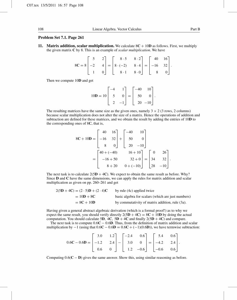
11. Matrix addition, scalar multiplication. We calculate 8C + 10D as follows. First, we multiplythe given matrix C by 8. This is an example of scalar multiplication. We have
8C = 8
5 2
−2 4
1 0
=
8 · 5 8 · 2
8 · (−2) 8 · 4
8 · 1 8 · 0
=
40 16
−16 32
8 0
.
Then we compute 10D and get
10D = 10
−4 1
5 0
2 −1
=
−40 10
50 0
20 −10
.
The resulting matrices have the same size as the given ones, namely 3 × 2 (3 rows, 2 columns)because scalar multiplication does not alter the size of a matrix. Hence the operations of addition andsubtraction are defined for these matrices, and we obtain the result by adding the entries of 10D tothe corresponding ones of 8C, that is,
8C + 10D =
40 16
−16 32
8 0
+
−40 10
50 0
20 −10
=
40 + (−40) 16 + 10
−16 + 50 32 + 0
8 + 20 0 + (−10)
=
0 26
34 32
28 −10
.
The next task is to calculate 2(5D + 4C). We expect to obtain the same result as before. Why?Since D and C have the same dimensions, we can apply the rules for matrix addition and scalarmultiplication as given on pp. 260–261 and get
2(5D + 4C) = (2 · 5)D + (2 · 4)C by rule (4c) applied twice
= 10D + 8C basic algebra for scalars (which are just numbers)
= 8C + 10D by commutativity of matrix addition, rule (3a).
Having given a general abstract algebraic derivation (which is a formal proof!) as to why weexpect the same result, you should verify directly 2(5D + 4C) = 8C + 10D by doing the actualcomputation. You should calculate 5D, 4C, 5D + 4C and finally 2(5D + 4C) and compare.
The next task is to compute 0.6C − 0.6D. Thus, from the definition of matrix addition and scalarmultiplication by −1 (using that 0.6C − 0.6D = 0.6C + (−1)(0.6D)), we have termwise subtraction:
0.6C − 0.6D =
3.0 1.2
−1.2 2.4
0.6 0
−
−2.4 0.6
3.0 0
1.2 −0.6
=
5.4 0.6
−4.2 2.4
−0.6 0.6
.
Computing 0.6(C − D) gives the same answer. Show this, using similar reasoning as before.
C07.tex 13/5/2011 16: 57 Page 109
Chap. 7 Linear Algebra: Matrices, Vectors, Determinants. Linear Systems 109
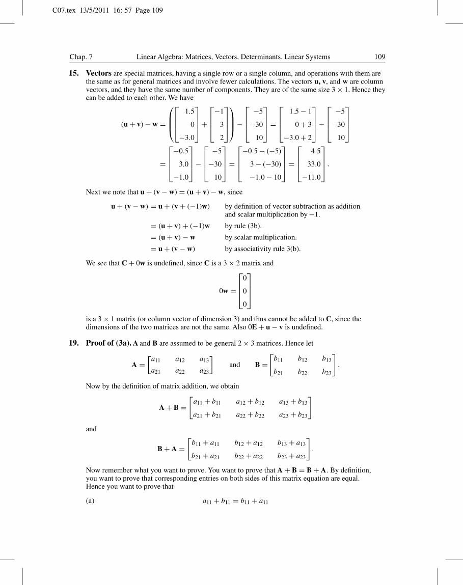
15. Vectors are special matrices, having a single row or a single column, and operations with them arethe same as for general matrices and involve fewer calculations. The vectors u, v, and w are columnvectors, and they have the same number of components. They are of the same size 3 × 1. Hence theycan be added to each other. We have
(u + v) − w =
1.5
0
−3.0
+
−1
3
2
−
−5
−30
10
=
1.5 − 1
0 + 3
−3.0 + 2
−
−5
−30
10
=
−0.5
3.0
−1.0
−
−5
−30
10
=
−0.5 − (−5)
3 − (−30)
−1.0 − 10
=
4.5
33.0
−11.0
.
Next we note that u + (v − w) = (u + v) − w, since
u + (v − w) = u + (v + (−1)w) by definition of vector subtraction as additionand scalar multiplication by −1.
= (u + v) + (−1)w by rule (3b).
= (u + v) − w by scalar multiplication.
= u + (v − w) by associativity rule 3(b).
We see that C + 0w is undefined, since C is a 3 × 2 matrix and
0w =
0
0
0
is a 3 × 1 matrix (or column vector of dimension 3) and thus cannot be added to C, since thedimensions of the two matrices are not the same. Also 0E + u − v is undefined.
19. Proof of (3a). A and B are assumed to be general 2 × 3 matrices. Hence let
A =[
a11 a12 a13
a21 a22 a23
]and B =
[b11 b12 b13
b21 b22 b23
].
Now by the definition of matrix addition, we obtain
A + B =[
a11 + b11 a12 + b12 a13 + b13
a21 + b21 a22 + b22 a23 + b23
]and
B + A =[
b11 + a11 b12 + a12 b13 + a13
b21 + a21 b22 + a22 b23 + a23
].
Now remember what you want to prove. You want to prove that A + B = B + A. By definition,you want to prove that corresponding entries on both sides of this matrix equation are equal.Hence you want to prove that
(a) a11 + b11 = b11 + a11
C07.tex 13/5/2011 16: 57 Page 110
110 Linear Algebra. Vector Calculus Part B
and similarly for the other five pairs of entries. Now comes the idea, the key of the proof. Use thecommutativity of the addition of numbers to conclude that the two sides of (a) are equal. Similarlyfor the other five pairs of entries. This completes the proof.
The proofs of all the other formulas in (3) of p. 260 and (4) of p. 261 follow the same pattern andthe same idea. Perform all these proofs to make sure that you really understand the logic of ourprocedure of proving such general matrix formulas. In each case, the equality of matrices followsfrom the corresponding property for the equality of numbers.
Sec. 7.2 Matrix Multiplication
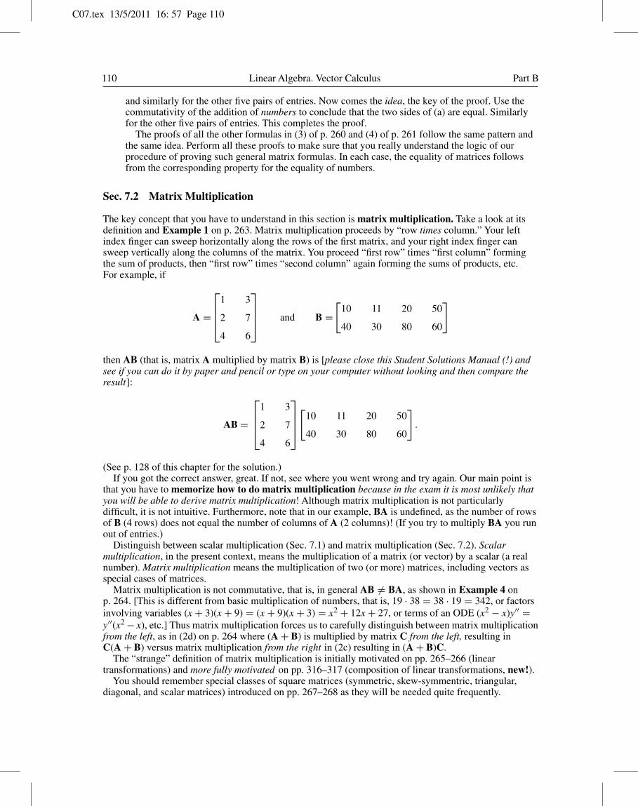
The key concept that you have to understand in this section is matrix multiplication. Take a look at itsdefinition and Example 1 on p. 263. Matrix multiplication proceeds by “row times column.” Your leftindex finger can sweep horizontally along the rows of the first matrix, and your right index finger cansweep vertically along the columns of the matrix. You proceed “first row” times “first column” formingthe sum of products, then “first row” times “second column” again forming the sums of products, etc.For example, if
A =
1 3
2 7
4 6
and B =[
10 11 20 50
40 30 80 60
]
then AB (that is, matrix A multiplied by matrix B) is [please close this Student Solutions Manual (!) andsee if you can do it by paper and pencil or type on your computer without looking and then compare theresult]:
AB =
1 3
2 7
4 6
[
10 11 20 50
40 30 80 60
].
(See p. 128 of this chapter for the solution.)If you got the correct answer, great. If not, see where you went wrong and try again. Our main point is
that you have to memorize how to do matrix multiplication because in the exam it is most unlikely thatyou will be able to derive matrix multiplication! Although matrix multiplication is not particularlydifficult, it is not intuitive. Furthermore, note that in our example, BA is undefined, as the number of rowsof B (4 rows) does not equal the number of columns of A (2 columns)! (If you try to multiply BA you runout of entries.)
Distinguish between scalar multiplication (Sec. 7.1) and matrix multiplication (Sec. 7.2). Scalarmultiplication, in the present context, means the multiplication of a matrix (or vector) by a scalar (a realnumber). Matrix multiplication means the multiplication of two (or more) matrices, including vectors asspecial cases of matrices.
Matrix multiplication is not commutative, that is, in general AB �= BA, as shown in Example 4 onp. 264. [This is different from basic multiplication of numbers, that is, 19 · 38 = 38 · 19 = 342, or factorsinvolving variables (x + 3)(x + 9) = (x + 9)(x + 3) = x2 + 12x + 27, or terms of an ODE (x2 − x)y′′ =y′′(x2 − x), etc.] Thus matrix multiplication forces us to carefully distinguish between matrix multiplicationfrom the left, as in (2d) on p. 264 where (A + B) is multiplied by matrix C from the left, resulting inC(A + B) versus matrix multiplication from the right in (2c) resulting in (A + B)C.
The “strange” definition of matrix multiplication is initially motivated on pp. 265–266 (lineartransformations) and more fully motivated on pp. 316–317 (composition of linear transformations, new!).
You should remember special classes of square matrices (symmetric, skew-symmentric, triangular,diagonal, and scalar matrices) introduced on pp. 267–268 as they will be needed quite frequently.
C07.tex 13/5/2011 16: 57 Page 111
Chap. 7 Linear Algebra: Matrices, Vectors, Determinants. Linear Systems 111
Problem Set 7.2. Page 270
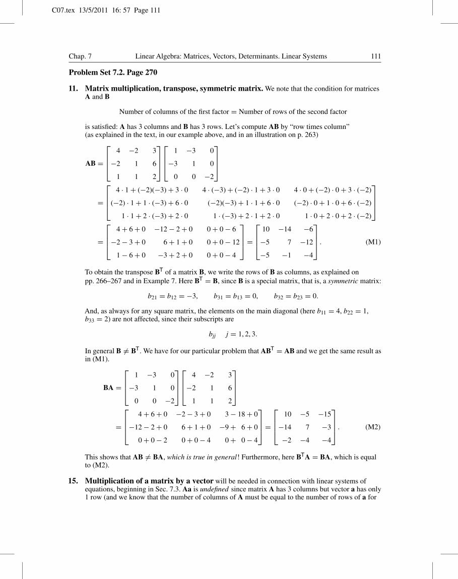
11. Matrix multiplication, transpose, symmetric matrix. We note that the condition for matricesA and B
Number of columns of the first factor = Number of rows of the second factor
is satisfied: A has 3 columns and B has 3 rows. Let’s compute AB by “row times column”(as explained in the text, in our example above, and in an illustration on p. 263)
AB =
4 −2 3
−2 1 6
1 1 2
1 −3 0
−3 1 0
0 0 −2
=
4 · 1 + (−2)(−3) + 3 · 0 4 · (−3) + (−2) · 1 + 3 · 0 4 · 0 + (−2) · 0 + 3 · (−2)
(−2) · 1 + 1 · (−3) + 6 · 0 (−2)(−3) + 1 · 1 + 6 · 0 (−2) · 0 + 1 · 0 + 6 · (−2)
1 · 1 + 2 · (−3) + 2 · 0 1 · (−3) + 2 · 1 + 2 · 0 1 · 0 + 2 · 0 + 2 · (−2)
=
4 + 6 + 0 −12 − 2 + 0 0 + 0 − 6
−2 − 3 + 0 6 + 1 + 0 0 + 0 − 12
1 − 6 + 0 −3 + 2 + 0 0 + 0 − 4
=
10 −14 −6
−5 7 −12
−5 −1 −4
. (M1)
To obtain the transpose BT of a matrix B, we write the rows of B as columns, as explained onpp. 266–267 and in Example 7. Here BT = B, since B is a special matrix, that is, a symmetric matrix:
b21 = b12 = −3, b31 = b13 = 0, b32 = b23 = 0.
And, as always for any square matrix, the elements on the main diagonal (here b11 = 4, b22 = 1,b33 = 2) are not affected, since their subscripts are
bjj j = 1, 2, 3.
In general B �= BT. We have for our particular problem that ABT = AB and we get the same result asin (M1).
BA =
1 −3 0
−3 1 0
0 0 −2
4 −2 3
−2 1 6
1 1 2
=
4 + 6 + 0 −2 − 3 + 0 3 − 18 + 0
−12 − 2 + 0 6 + 1 + 0 −9 + 6 + 0
0 + 0 − 2 0 + 0 − 4 0 + 0 − 4
=
10 −5 −15
−14 7 −3
−2 −4 −4
. (M2)
This shows that AB �= BA, which is true in general! Furthermore, here BTA = BA, which is equalto (M2).
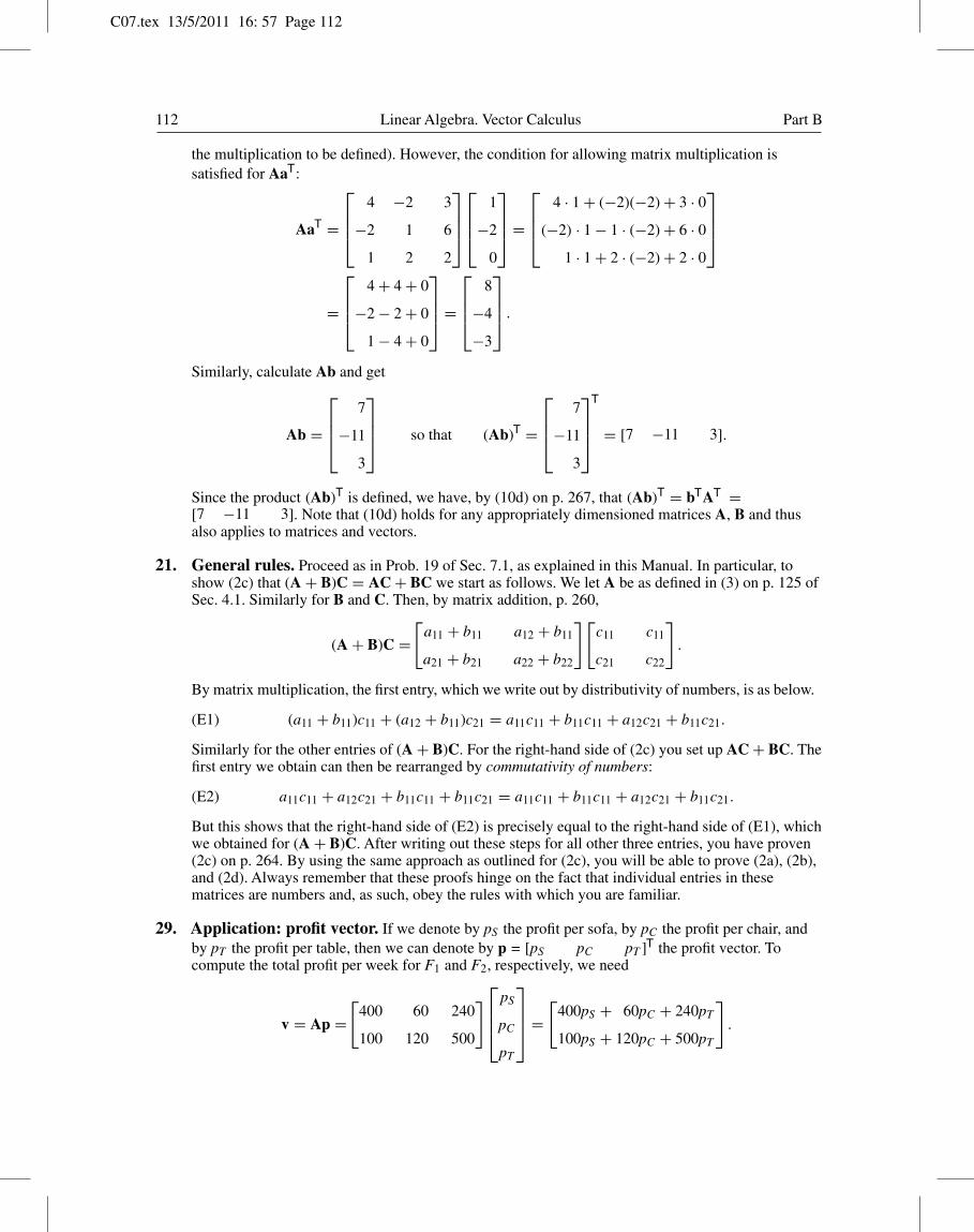
15. Multiplication of a matrix by a vector will be needed in connection with linear systems ofequations, beginning in Sec. 7.3. Aa is undefined since matrix A has 3 columns but vector a has only1 row (and we know that the number of columns of A must be equal to the number of rows of a for
C07.tex 13/5/2011 16: 57 Page 112
112 Linear Algebra. Vector Calculus Part B
the multiplication to be defined). However, the condition for allowing matrix multiplication issatisfied for AaT:
AaT =
4 −2 3
−2 1 6
1 2 2
1
−2
0
=
4 · 1 + (−2)(−2) + 3 · 0
(−2) · 1 − 1 · (−2) + 6 · 0
1 · 1 + 2 · (−2) + 2 · 0
=
4 + 4 + 0
−2 − 2 + 0
1 − 4 + 0
=
8
−4
−3
.
Similarly, calculate Ab and get
Ab =
7
−11
3
so that (Ab)T =
7
−11
3
T
= [7 −11 3].
Since the product (Ab)T is defined, we have, by (10d) on p. 267, that (Ab)T = bTAT =[7 −11 3]. Note that (10d) holds for any appropriately dimensioned matrices A, B and thusalso applies to matrices and vectors.
21. General rules. Proceed as in Prob. 19 of Sec. 7.1, as explained in this Manual. In particular, toshow (2c) that (A + B)C = AC + BC we start as follows. We let A be as defined in (3) on p. 125 ofSec. 4.1. Similarly for B and C. Then, by matrix addition, p. 260,
(A + B)C =[
a11 + b11 a12 + b11
a21 + b21 a22 + b22
] [c11 c11
c21 c22
].
By matrix multiplication, the first entry, which we write out by distributivity of numbers, is as below.
(E1) (a11 + b11)c11 + (a12 + b11)c21 = a11c11 + b11c11 + a12c21 + b11c21.
Similarly for the other entries of (A + B)C. For the right-hand side of (2c) you set up AC + BC. Thefirst entry we obtain can then be rearranged by commutativity of numbers:
(E2) a11c11 + a12c21 + b11c11 + b11c21 = a11c11 + b11c11 + a12c21 + b11c21.
But this shows that the right-hand side of (E2) is precisely equal to the right-hand side of (E1), whichwe obtained for (A + B)C. After writing out these steps for all other three entries, you have proven(2c) on p. 264. By using the same approach as outlined for (2c), you will be able to prove (2a), (2b),and (2d). Always remember that these proofs hinge on the fact that individual entries in thesematrices are numbers and, as such, obey the rules with which you are familiar.
29. Application: profit vector. If we denote by pS the profit per sofa, by pC the profit per chair, andby pT the profit per table, then we can denote by p = [pS pC pT ]T the profit vector. Tocompute the total profit per week for F1 and F2, respectively, we need
v = Ap =[
400 60 240
100 120 500
] pS
pC
pT
=[
400pS + 60pC + 240pT
100pS + 120pC + 500pT
].
C07.tex 13/5/2011 16: 57 Page 113
Chap. 7 Linear Algebra: Matrices, Vectors, Determinants. Linear Systems 113
We are given that
pS = $85, pC = $62, pT = $30,
so that
v = Ap =[
400pS + 60pC + 240pT
100pS + 120pC + 500pT
]=
[400 · $85 + 60 · $62 + 240 · $30
100 · $85 + 120 · $62 + 500 · $30
].
This simplifies to [$44,920 $30,940]T as given on p. A17.
Sec. 7.3 Linear Systems of Equations. Gauss Elimination
This is the heart of Chap. 7. Take a careful look at Example 2 on pp. 275–276. First you do Gausselimination. This involves changing the augmented matrix A (also preferably denoted by [A | b] onp. 279) to an upper triangular matrix (4) by elementary row operations. They are (p. 277) interchange oftwo equations (rows), addition of a constant multiple of one equation (row) to another equation (row), andmultiplication of an equation (a row) by a nonzero constant c. The method involves the strategy of“eliminating” (“reducing to 0”) all entries in the augmented matrix that are below the main diagonal. Youobtain matrix (4). Then you do back substitution. Problem 3 of this section gives another carefullyexplained example.
A system of linear equations can have a unique solution (Example 2, pp. 275–276), infinitely manysolutions (Example 3, p. 278), and no solution (Example 4, pp. 278–279).
Look at Example 4. No solution arises because Gauss gives us “0 = 12,” that is, “0x3 = 12,” which isimpossible to solve. The equations have no point in common. The geometric meaning is parallel planes(Fig. 158) or, in two dimensions, parallel lines. You need to practice the important technique of Gausselimination and back substitution. Indeed, Sec. 7.3 serves as the background for the theory of Secs. 7.4 and7.5. Gauss elimination appears in many variants, such as in computing inverses of matrices (Sec. 7.8, calledGauss–Jordan method) and in solving elliptic PDEs numerically (Sec. 21.4, called Liebmann’s method).
Problem Set 7.3. Page 280
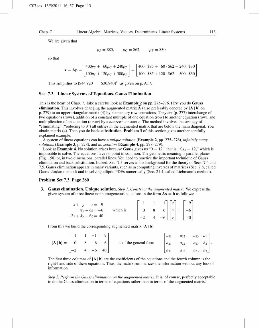
3. Gauss elimination. Unique solution. Step 1. Construct the augmented matrix. We express thegiven system of three linear nonhomogeneous equations in the form Ax = b as follows:
x + y − z = 98y + 6z = −6
−2x + 4y − 6z = 40
which is
1 1 −1
0 8 6
−2 4 −6
x
y
z
=
9
−6
40
.
From this we build the corresponding augmented matrix [A | b]:
[A | b] =
1 1 −1
0 8 6
−2 4 −6
9
−6
40
is of the general form
a11 a12 a13
a21 a22 a23
a31 a32 a33
b1
b2
b3
.
The first three columns of [A | b] are the coefficients of the equations and the fourth column is theright-hand side of these equations. Thus, the matrix summarizes the information without any loss ofinformation.
Step 2. Perform the Gauss elimination on the augmented matrix. It is, of course, perfectly acceptableto do the Gauss elimination in terms of equations rather than in terms of the augmented matrix.
C07.tex 13/5/2011 16: 57 Page 114
114 Linear Algebra. Vector Calculus Part B
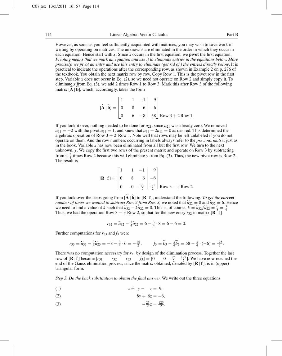
However, as soon as you feel sufficiently acquainted with matrices, you may wish to save work inwriting by operating on matrices. The unknowns are eliminated in the order in which they occur ineach equation. Hence start with x. Since x occurs in the first equation, we pivot the first equation.Pivoting means that we mark an equation and use it to eliminate entries in the equations below. Moreprecisely, we pivot an entry and use this entry to eliminate (get rid of ) the entries directly below. It ispractical to indicate the operations after the corresponding row, as shown in Example 2 on p. 276 ofthe textbook. You obtain the next matrix row by row. Copy Row 1. This is the pivot row in the firststep. Variable x does not occur in Eq. (2), so we need not operate on Row 2 and simply copy it. Toeliminate x from Eq. (3), we add 2 times Row 1 to Row 3. Mark this after Row 3 of the followingmatrix [A | b], which, accordingly, takes the form
[A | b] =
1 1 −1
0 8 6
0 6 −8
9
−6
58
Row 3 + 2 Row 1.
If you look it over, nothing needed to be done for a21, since a21 was already zero. We removeda31 = −2 with the pivot a11 = 1, and knew that a31 + 2a11 = 0 as desired. This determined thealgebraic operation of Row 3 + 2 Row 1. Note well that rows may be left unlabeled if you do notoperate on them. And the row numbers occurring in labels always refer to the previous matrix just asin the book. Variable x has now been eliminated from all but the first row. We turn to the nextunknown, y. We copy the first two rows of the present matrix and operate on Row 3 by subtractingfrom it 3
4 times Row 2 because this will eliminate y from Eq. (3). Thus, the new pivot row is Row 2.The result is
[R | f ] =
1 1 −1
0 8 6
0 0 −252
9
−6
1252
Row 3 − 3
4 Row 2.
If you look over the steps going from [A | b] to [R | f ], understand the following. To get the correctnumber of times we wanted to subtract Row 2 from Row 3, we noted that a22 = 8 and a32 = 6. Hencewe need to find a value of k such that a32 − ka22 = 0. This is, of course, k = a32/a22 = 6
8 = 34 .
Thus, we had the operation Row 3 − 34 Row 2, so that for the new entry r32 in matrix [R | f ]
r32 = a32 − 34 a22 = 6 − 3
4 · 8 = 6 − 6 = 0.
Further computations for r33 and f3 were
r33 = a33 − 34 a23 = −8 − 3
4 · 6 = −252 ; f3 = b3 − 3
4 b2 = 58 − 34 · (−6) = 125
2 .
There was no computation necessary for r31 by design of the elimination process. Together the lastrow of [R | f ] became [r31 r32 r33 f3] = [0 0 −25
2125
2 ]. We have now reached theend of the Gauss elimination process, since the matrix obtained, denoted by [R | f ], is in (upper)triangular form.
Step 3. Do the back substitution to obtain the final answer. We write out the three equations
x + y − z = 9,(1)
8y + 6z = −6,(2)
−252 z = 125
2 .(3)
C07.tex 13/5/2011 16: 57 Page 115
Chap. 7 Linear Algebra: Matrices, Vectors, Determinants. Linear Systems 115
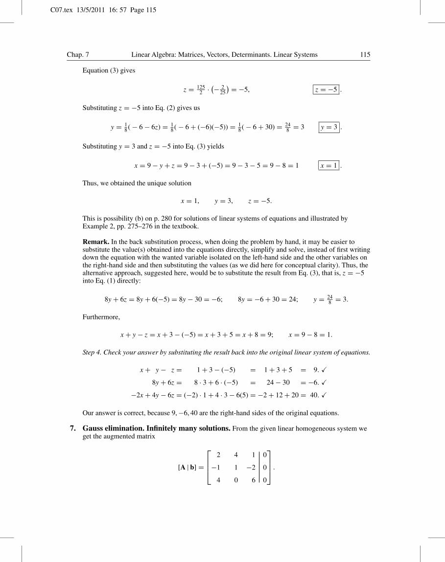
Equation (3) gives
z = 1252 · (− 2
25
) = −5, z = −5 .
Substituting z = −5 into Eq. (2) gives us
y = 18 ( − 6 − 6z) = 1
8 ( − 6 + (−6)(−5)) = 18 ( − 6 + 30) = 24
8 = 3 y = 3 .
Substituting y = 3 and z = −5 into Eq. (3) yields
x = 9 − y + z = 9 − 3 + (−5) = 9 − 3 − 5 = 9 − 8 = 1 x = 1 .
Thus, we obtained the unique solution
x = 1, y = 3, z = −5.
This is possibility (b) on p. 280 for solutions of linear systems of equations and illustrated byExample 2, pp. 275–276 in the textbook.
Remark. In the back substitution process, when doing the problem by hand, it may be easier tosubstitute the value(s) obtained into the equations directly, simplify and solve, instead of first writingdown the equation with the wanted variable isolated on the left-hand side and the other variables onthe right-hand side and then substituting the values (as we did here for conceptual clarity). Thus, thealternative approach, suggested here, would be to substitute the result from Eq. (3), that is, z = −5into Eq. (1) directly:
8y + 6z = 8y + 6(−5) = 8y − 30 = −6; 8y = −6 + 30 = 24; y = 248 = 3.
Furthermore,
x + y − z = x + 3 − (−5) = x + 3 + 5 = x + 8 = 9; x = 9 − 8 = 1.
Step 4. Check your answer by substituting the result back into the original linear system of equations.
x + y − z = 1 + 3 − (−5) = 1 + 3 + 5 = 9. �8y + 6z = 8 · 3 + 6 · (−5) = 24 − 30 = −6. �
−2x + 4y − 6z = (−2) · 1 + 4 · 3 − 6(5) = −2 + 12 + 20 = 40. �
Our answer is correct, because 9, −6, 40 are the right-hand sides of the original equations.
7. Gauss elimination. Infinitely many solutions. From the given linear homogeneous system weget the augmented matrix
[A | b] =
2 4 1
−1 1 −2
4 0 6
0
0
0
.
C07.tex 13/5/2011 16: 57 Page 116
116 Linear Algebra. Vector Calculus Part B
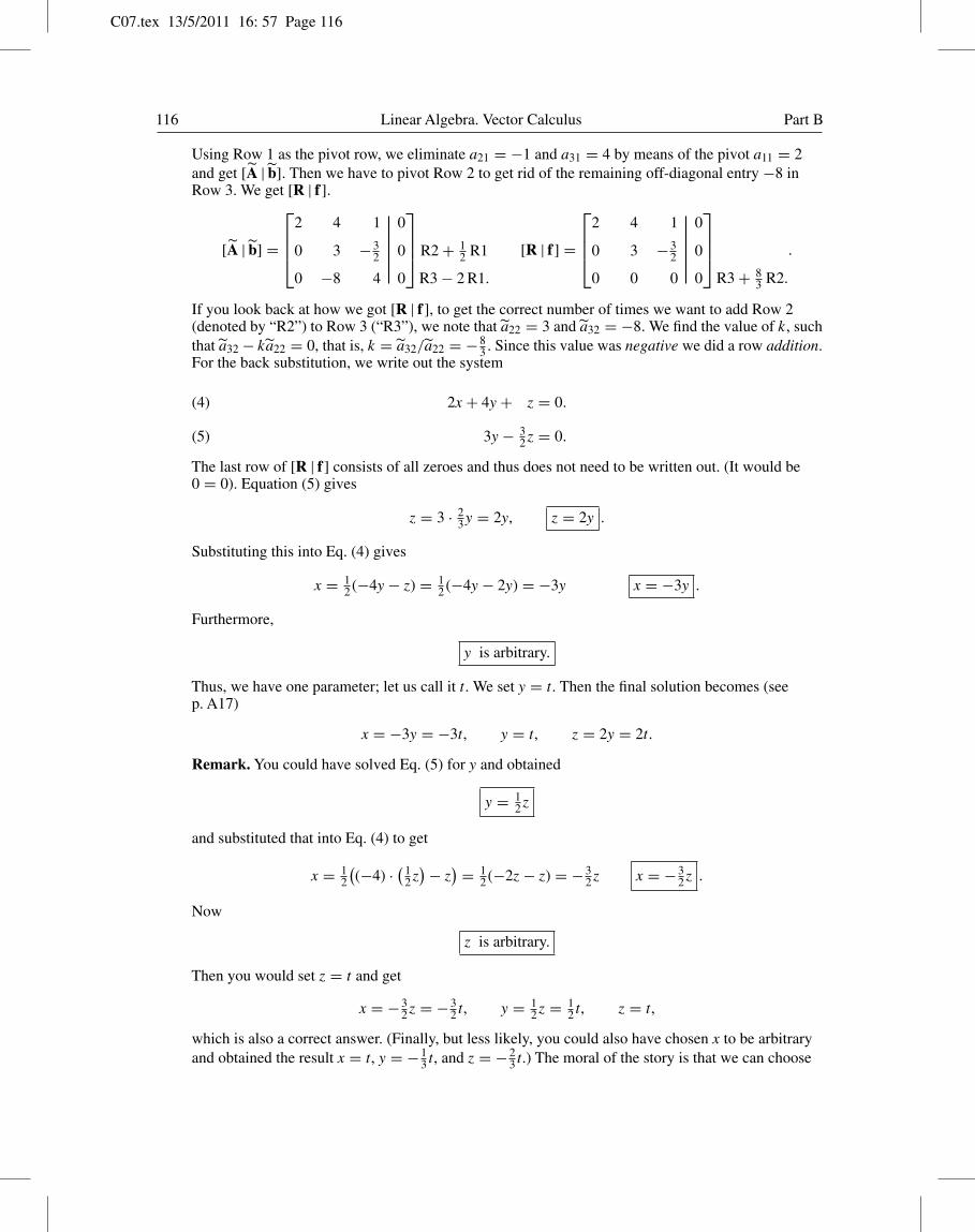
Using Row 1 as the pivot row, we eliminate a21 = −1 and a31 = 4 by means of the pivot a11 = 2and get [A | b]. Then we have to pivot Row 2 to get rid of the remaining off-diagonal entry −8 inRow 3. We get [R | f ].
[A | b] =
2 4 1
0 3 −32
0 −8 4
0
0
0
R2 + 12 R1
R3 − 2 R1.
[R | f ] =
2 4 1
0 3 −32
0 0 0
0
0
0
R3 + 8
3 R2.
.
If you look back at how we got [R | f ], to get the correct number of times we want to add Row 2(denoted by “R2”) to Row 3 (“R3”), we note that a22 = 3 and a32 = −8. We find the value of k, suchthat a32 − ka22 = 0, that is, k = a32/a22 = −8
3 . Since this value was negative we did a row addition.For the back substitution, we write out the system
2x + 4y + z = 0.(4)
3y − 32z = 0.(5)
The last row of [R | f ] consists of all zeroes and thus does not need to be written out. (It would be0 = 0). Equation (5) gives
z = 3 · 23y = 2y, z = 2y .
Substituting this into Eq. (4) gives
x = 12 (−4y − z) = 1
2 (−4y − 2y) = −3y x = −3y .
Furthermore,
y is arbitrary.
Thus, we have one parameter; let us call it t. We set y = t. Then the final solution becomes (seep. A17)
x = −3y = −3t, y = t, z = 2y = 2t.
Remark. You could have solved Eq. (5) for y and obtained
y = 12z
and substituted that into Eq. (4) to get
x = 12
((−4) · (1
2z) − z
) = 12 (−2z − z) = −3
2z x = −32z .
Now
z is arbitrary.
Then you would set z = t and get
x = −32z = −3
2 t, y = 12z = 1
2 t, z = t,
which is also a correct answer. (Finally, but less likely, you could also have chosen x to be arbitraryand obtained the result x = t, y = −1
3 t, and z = −23 t.) The moral of the story is that we can choose
C07.tex 13/5/2011 16: 57 Page 117
Chap. 7 Linear Algebra: Matrices, Vectors, Determinants. Linear Systems 117
which variable we set to the parameter t with one choice allowed in this problem. This exampleillustrates possibility (c) on p. 280 in the textbook, that is, infinitely many solutions (as we can chooseany value for the parameter t and thus have infinitely many choices for t) and Example 3 on p. 278.
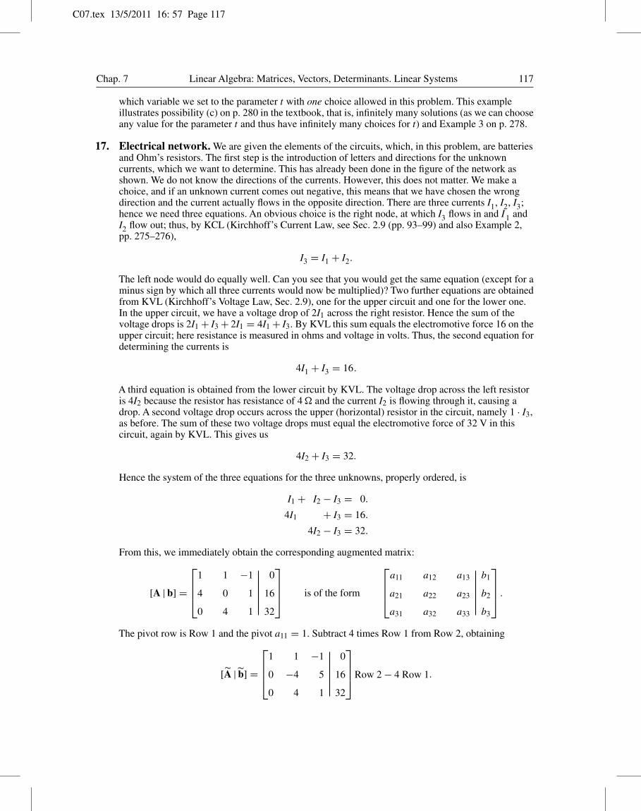
17. Electrical network. We are given the elements of the circuits, which, in this problem, are batteriesand Ohm’s resistors. The first step is the introduction of letters and directions for the unknowncurrents, which we want to determine. This has already been done in the figure of the network asshown. We do not know the directions of the currents. However, this does not matter. We make achoice, and if an unknown current comes out negative, this means that we have chosen the wrongdirection and the current actually flows in the opposite direction. There are three currents I1, I2, I3;hence we need three equations. An obvious choice is the right node, at which I3 flows in and I1 andI2 flow out; thus, by KCL (Kirchhoff’s Current Law, see Sec. 2.9 (pp. 93–99) and also Example 2,pp. 275–276),
I3 = I1 + I2.
The left node would do equally well. Can you see that you would get the same equation (except for aminus sign by which all three currents would now be multiplied)? Two further equations are obtainedfrom KVL (Kirchhoff’s Voltage Law, Sec. 2.9), one for the upper circuit and one for the lower one.In the upper circuit, we have a voltage drop of 2I1 across the right resistor. Hence the sum of thevoltage drops is 2I1 + I3 + 2I1 = 4I1 + I3. By KVL this sum equals the electromotive force 16 on theupper circuit; here resistance is measured in ohms and voltage in volts. Thus, the second equation fordetermining the currents is
4I1 + I3 = 16.
A third equation is obtained from the lower circuit by KVL. The voltage drop across the left resistoris 4I2 because the resistor has resistance of 4 � and the current I2 is flowing through it, causing adrop. A second voltage drop occurs across the upper (horizontal) resistor in the circuit, namely 1 · I3,as before. The sum of these two voltage drops must equal the electromotive force of 32 V in thiscircuit, again by KVL. This gives us
4I2 + I3 = 32.
Hence the system of the three equations for the three unknowns, properly ordered, is
I1 + I2 − I3 = 0.
4I1 + I3 = 16.
4I2 − I3 = 32.
From this, we immediately obtain the corresponding augmented matrix:
[A | b] =
1 1 −1
4 0 1
0 4 1
0
16
32
is of the form
a11 a12 a13
a21 a22 a23
a31 a32 a33
b1
b2
b3
.
The pivot row is Row 1 and the pivot a11 = 1. Subtract 4 times Row 1 from Row 2, obtaining
[A | b] =
1 1 −1
0 −4 5
0 4 1
0
16
32
Row 2 − 4 Row 1.
C07.tex 13/5/2011 16: 57 Page 118
118 Linear Algebra. Vector Calculus Part B
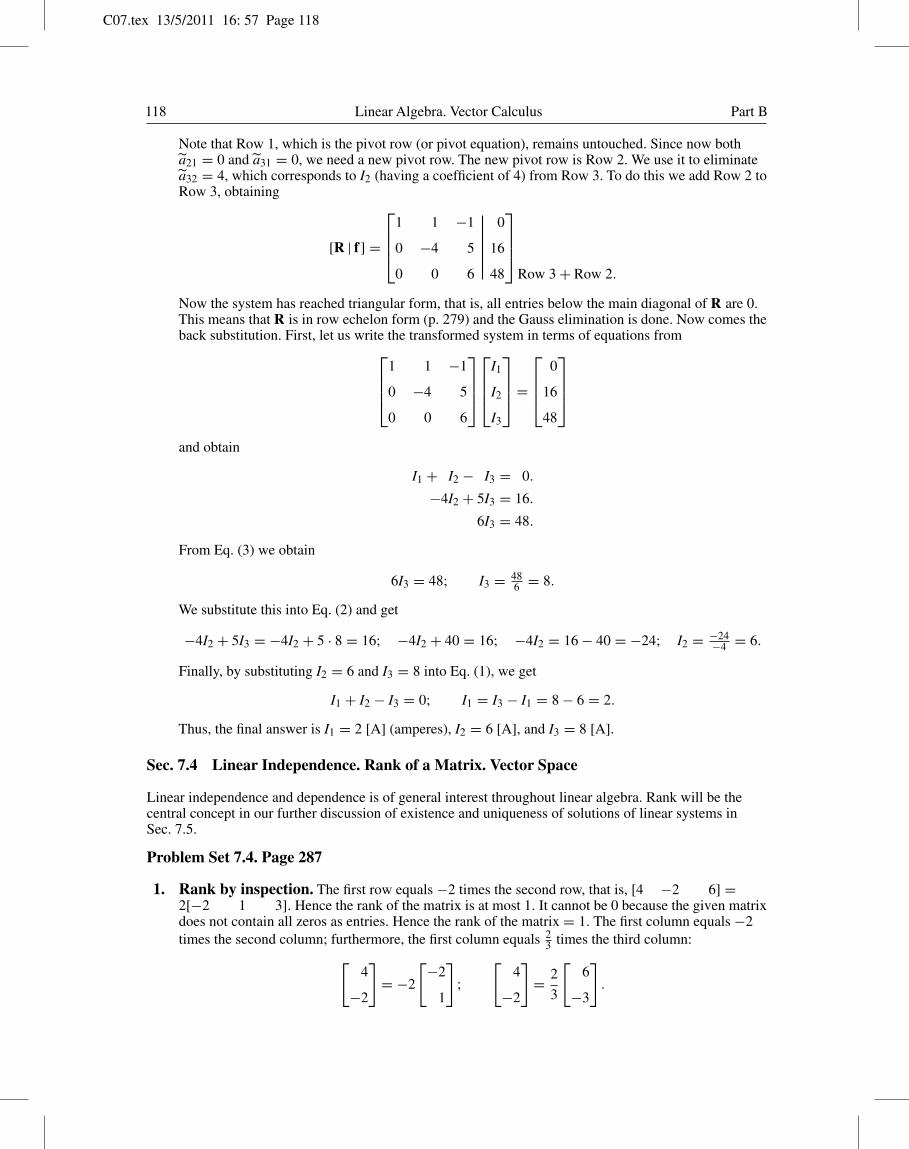
Note that Row 1, which is the pivot row (or pivot equation), remains untouched. Since now botha21 = 0 and a31 = 0, we need a new pivot row. The new pivot row is Row 2. We use it to eliminatea32 = 4, which corresponds to I2 (having a coefficient of 4) from Row 3. To do this we add Row 2 toRow 3, obtaining
[R | f ] =
1 1 −1
0 −4 5
0 0 6
0
16
48
Row 3 + Row 2.
Now the system has reached triangular form, that is, all entries below the main diagonal of R are 0.This means that R is in row echelon form (p. 279) and the Gauss elimination is done. Now comes theback substitution. First, let us write the transformed system in terms of equations from
1 1 −1
0 −4 5
0 0 6
I1
I2
I3
=
0
16
48
and obtain
I1 + I2 − I3 = 0.
−4I2 + 5I3 = 16.
6I3 = 48.
From Eq. (3) we obtain
6I3 = 48; I3 = 486 = 8.
We substitute this into Eq. (2) and get
−4I2 + 5I3 = −4I2 + 5 · 8 = 16; −4I2 + 40 = 16; −4I2 = 16 − 40 = −24; I2 = −24−4 = 6.
Finally, by substituting I2 = 6 and I3 = 8 into Eq. (1), we get
I1 + I2 − I3 = 0; I1 = I3 − I1 = 8 − 6 = 2.
Thus, the final answer is I1 = 2 [A] (amperes), I2 = 6 [A], and I3 = 8 [A].
Sec. 7.4 Linear Independence. Rank of a Matrix. Vector Space
Linear independence and dependence is of general interest throughout linear algebra. Rank will be thecentral concept in our further discussion of existence and uniqueness of solutions of linear systems inSec. 7.5.
Problem Set 7.4. Page 287
1. Rank by inspection. The first row equals −2 times the second row, that is, [4 −2 6] =2[−2 1 3]. Hence the rank of the matrix is at most 1. It cannot be 0 because the given matrixdoes not contain all zeros as entries. Hence the rank of the matrix = 1. The first column equals −2times the second column; furthermore, the first column equals 2
3 times the third column:[4
−2
]= −2
[−2
1
];
[4
−2
]= 2
3
[6
−3
].
C07.tex 13/5/2011 16: 57 Page 119
Chap. 7 Linear Algebra: Matrices, Vectors, Determinants. Linear Systems 119
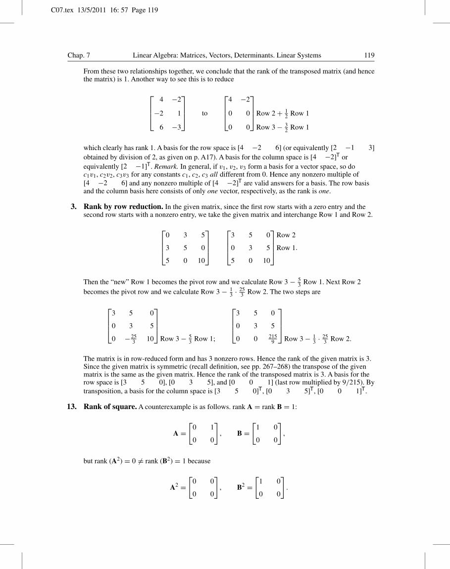
From these two relationships together, we conclude that the rank of the transposed matrix (and hencethe matrix) is 1. Another way to see this is to reduce
4 −2
−2 1
6 −3
to
4 −2
0 0
0 0
Row 2 + 12 Row 1
Row 3 − 32 Row 1
which clearly has rank 1. A basis for the row space is [4 −2 6] (or equivalently [2 −1 3]obtained by division of 2, as given on p. A17). A basis for the column space is [4 −2]T orequivalently [2 −1]T. Remark. In general, if v1, v2, v3 form a basis for a vector space, so doc1v1, c2v2, c3v3 for any constants c1, c2, c3 all different from 0. Hence any nonzero multiple of[4 −2 6] and any nonzero multiple of [4 −2]T are valid answers for a basis. The row basisand the column basis here consists of only one vector, respectively, as the rank is one.
3. Rank by row reduction. In the given matrix, since the first row starts with a zero entry and thesecond row starts with a nonzero entry, we take the given matrix and interchange Row 1 and Row 2.
0 3 5
3 5 0
5 0 10
3 5 0
0 3 5
5 0 10
Row 2
Row 1.
Then the “new” Row 1 becomes the pivot row and we calculate Row 3 − 53 Row 1. Next Row 2
becomes the pivot row and we calculate Row 3 − 13 · 25
3 Row 2. The two steps are
3 5 0
0 3 5
0 −253 10
Row 3 − 5
3 Row 1;
3 5 0
0 3 5
0 0 2159
Row 3 − 1
3 · 253 Row 2.
The matrix is in row-reduced form and has 3 nonzero rows. Hence the rank of the given matrix is 3.Since the given matrix is symmetric (recall definition, see pp. 267–268) the transpose of the givenmatrix is the same as the given matrix. Hence the rank of the transposed matrix is 3. A basis for therow space is [3 5 0], [0 3 5], and [0 0 1] (last row multiplied by 9/215). Bytransposition, a basis for the column space is [3 5 0]T, [0 3 5]T, [0 0 1]T.
13. Rank of square. A counterexample is as follows. rank A = rank B = 1:
A =[
0 1
0 0
], B =
[1 0
0 0
],
but rank (A2) = 0 �= rank (B2) = 1 because
A2 =[
0 0
0 0
], B2 =
[1 0
0 0
].
C07.tex 13/5/2011 16: 57 Page 120
120 Linear Algebra. Vector Calculus Part B
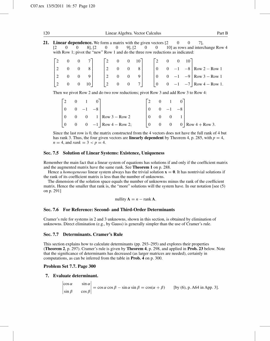
21. Linear dependence. We form a matrix with the given vectors [2 0 0 7],[2 0 0 8], [2 0 0 9], [2 0 0 10] as rows and interchange Row 4with Row 1; pivot the “new” Row 1 and do the three row reductions as indicated:
2 0 0 7
2 0 0 8
2 0 0 9
2 0 0 10
2 0 0 10
2 0 0 8
2 0 0 9
2 0 0 7
2 0 0 10
0 0 −1 −8
0 0 −1 −9
0 0 −1 −7
Row 2 − Row 1
Row 3 − Row 1
Row 4 − Row 1.
Then we pivot Row 2 and do two row reductions; pivot Row 3 and add Row 3 to Row 4:2 0 1 0
0 0 −1 −8
0 0 0 1
0 0 0 −1
Row 3 − Row 2
Row 4 − Row 2;
2 0 1 0
0 0 −1 −8
0 0 0 1
0 0 0 0
Row 4 + Row 3.
Since the last row is 0, the matrix constructed from the 4 vectors does not have the full rank of 4 buthas rank 3. Thus, the four given vectors are linearly dependent by Theorem 4, p. 285, with p = 4,n = 4, and rank = 3 < p = 4.
Sec. 7.5 Solution of Linear Systems: Existence, Uniqueness
Remember the main fact that a linear system of equations has solutions if and only if the coefficient matrixand the augmented matrix have the same rank. See Theorem 1 on p. 288.
Hence a homogeneous linear system always has the trivial solution x = 0. It has nontrivial solutions ifthe rank of its coefficient matrix is less than the number of unknowns.
The dimension of the solution space equals the number of unknowns minus the rank of the coefficientmatrix. Hence the smaller that rank is, the “more” solutions will the system have. In our notation [see (5)on p. 291]
nullity A = n − rank A.
Sec. 7.6 For Reference: Second- and Third-Order Determinants
Cramer’s rule for systems in 2 and 3 unknowns, shown in this section, is obtained by elimination ofunknowns. Direct elimination (e.g., by Gauss) is generally simpler than the use of Cramer’s rule.
Sec. 7.7 Determinants. Cramer’s Rule
This section explains how to calculate determinants (pp. 293–295) and explores their properties(Theorem 2, p. 297). Cramer’s rule is given by Theorem 4, p. 298, and applied in Prob. 23 below. Notethat the significance of determinants has decreased (as larger matrices are needed), certainly incomputations, as can be inferred from the table in Prob. 4 on p. 300.
Problem Set 7.7. Page 300
7. Evaluate determinant.∣∣∣∣∣cos α sin α
sin β cos β
∣∣∣∣∣ = cos α cos β − sin α sin β = cos(α + β) [by (6), p. A64 in App. 3].
C07.tex 13/5/2011 16: 57 Page 121
Chap. 7 Linear Algebra: Matrices, Vectors, Determinants. Linear Systems 121
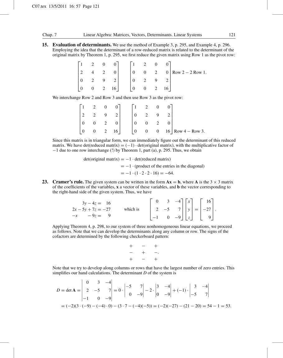
15. Evaluation of determinants. We use the method of Example 3, p. 295, and Example 4, p. 296.Employing the idea that the determinant of a row-reduced matrix is related to the determinant of theoriginal matrix by Theorem 1, p. 295, we first reduce the given matrix using Row 1 as the pivot row:
1 2 0 0
2 4 2 0
0 2 9 2
0 0 2 16
1 2 0 0
0 0 2 0
0 2 9 2
0 0 2 16
Row 2 − 2 Row 1.
We interchange Row 2 and Row 3 and then use Row 3 as the pivot row:1 2 0 0
2 2 9 2
0 0 2 0
0 0 2 16
1 2 0 0
0 2 9 2
0 0 2 0
0 0 0 16
Row 4 − Row 3.
Since this matrix is in triangular form, we can immediately figure out the determinant of this reducedmatrix. We have det(reduced matrix) = (−1) · det(original matrix), with the multiplicative factor of−1 due to one row interchange (!) by Theorem 1, part (a), p. 295. Thus, we obtain
det(original matrix) = −1 · det(reduced matrix)
= −1 · (product of the entries in the diagonal)
= −1 · (1 · 2 · 2 · 16) = −64.
23. Cramer’s rule. The given system can be written in the form Ax = b, where A is the 3 × 3 matrixof the coefficients of the variables, x a vector of these variables, and b the vector corresponding tothe right-hand side of the given system. Thus, we have
3y − 4z = 162x − 5y + 7z = −27−x − 9z = 9
which is
0 3 −4
2 −5 7
−1 0 −9
x
y
z
=
16
−27
9
.
Applying Theorem 4, p. 298, to our system of three nonhomogeneous linear equations, we proceedas follows. Note that we can develop the determinants along any column or row. The signs of thecofactors are determined by the following checkerboard pattern:
+ − +− + −+ − +
.
Note that we try to develop along columns or rows that have the largest number of zero entries. Thissimplifies our hand calculations. The determinant D of the system is
D = det A =
∣∣∣∣∣∣∣∣0 3 −4
2 −5 7
−1 0 −9
∣∣∣∣∣∣∣∣ = 0 ·∣∣∣∣∣−5 7
0 −9
∣∣∣∣∣ − 2 ·∣∣∣∣∣3 −4
0 −9
∣∣∣∣∣ + (−1) ·∣∣∣∣∣ 3 −4
−5 7
∣∣∣∣∣= (−2)(3 · (−9) − (−4) · 0) − (3 · 7 − (−4)(−5)) = (−2)(−27) − (21 − 20) = 54 − 1 = 53.
C07.tex 13/5/2011 16: 57 Page 122
122 Linear Algebra. Vector Calculus Part B
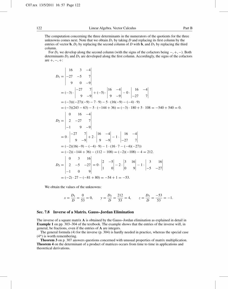
The computation concerning the three determinants in the numerators of the quotients for the threeunknowns comes next. Note that we obtain D1 by taking D and replacing its first column by theentries of vector b, D2 by replacing the second column of D with b, and D3 by replacing the thirdcolumn.
For D1 we develop along the second column (with the signs of the cofactors being −, +, −). Bothdeterminants D2 and D3 are developed along the first column. Accordingly, the signs of the cofactorsare +, −, +:
D1 =
∣∣∣∣∣∣∣∣16 3 −4
−27 −5 7
9 0 −9
∣∣∣∣∣∣∣∣= (−3) ·
∣∣∣∣∣−27 7
9 −9
∣∣∣∣∣ + (−5) ·∣∣∣∣∣16 −4
9 −9
∣∣∣∣∣ − 0 ·∣∣∣∣∣ 16 −4
−27 7
∣∣∣∣∣= (−3)((−27)(−9) − 7 · 9) − 5 · (16(−9) − (−4) · 9)
= (−3)(243 − 63) − 5 · (−144 + 36) = (−3) · 180 + 5 · 108 = −540 + 540 = 0.
D2 =
∣∣∣∣∣∣∣∣0 16 −4
2 −27 7
−1 9 −9
∣∣∣∣∣∣∣∣= 0 ·
∣∣∣∣∣−27 7
9 −9
∣∣∣∣∣ + 2 ·∣∣∣∣∣16 −4
9 −9
∣∣∣∣∣ − 1 ·∣∣∣∣∣ 16 −4
−27 7
∣∣∣∣∣= (−2)(16(−9) − (−4) · 9) − 1 · (16 · 7 − (−4)(−27))
= (−2)(−144 + 36) − (112 − 108) = (−2)(−108) − 4 = 212.
D3 =
∣∣∣∣∣∣∣∣0 3 16
2 −5 −27
−1 0 9
∣∣∣∣∣∣∣∣ = 0 ·∣∣∣∣∣2 −5
1 0
∣∣∣∣∣ − 2 ·∣∣∣∣∣3 16
0 9
∣∣∣∣∣ − 1 ·∣∣∣∣∣ 3 16
−5 −27
∣∣∣∣∣= (−2) · 27 − (−81 + 80) = −54 + 1 = −53.
We obtain the values of the unknowns:
x = D1
D= 0
53= 0, y = D2
D= 212
53= 4, z = D3
D= −53
53= −1.
Sec. 7.8 Inverse of a Matrix. Gauss–Jordan Elimination
The inverse of a square matrix A is obtained by the Gauss–Jordan elimination as explained in detail inExample 1 on pp. 303–304 of the textbook. The example shows that the entries of the inverse will, ingeneral, be fractions, even if the entries of A are integers.
The general formula (4) for the inverse (p. 304) is hardly needed in practice, whereas the special case(4*) is worth remembering.
Theorem 3 on p. 307 answers questions concerned with unusual properties of matrix multiplication.Theorem 4 on the determinant of a product of matrices occurs from time to time in applications andtheoretical derivations.
C07.tex 13/5/2011 16: 57 Page 123
Chap. 7 Linear Algebra: Matrices, Vectors, Determinants. Linear Systems 123
Problem Set 7.8. Page 308
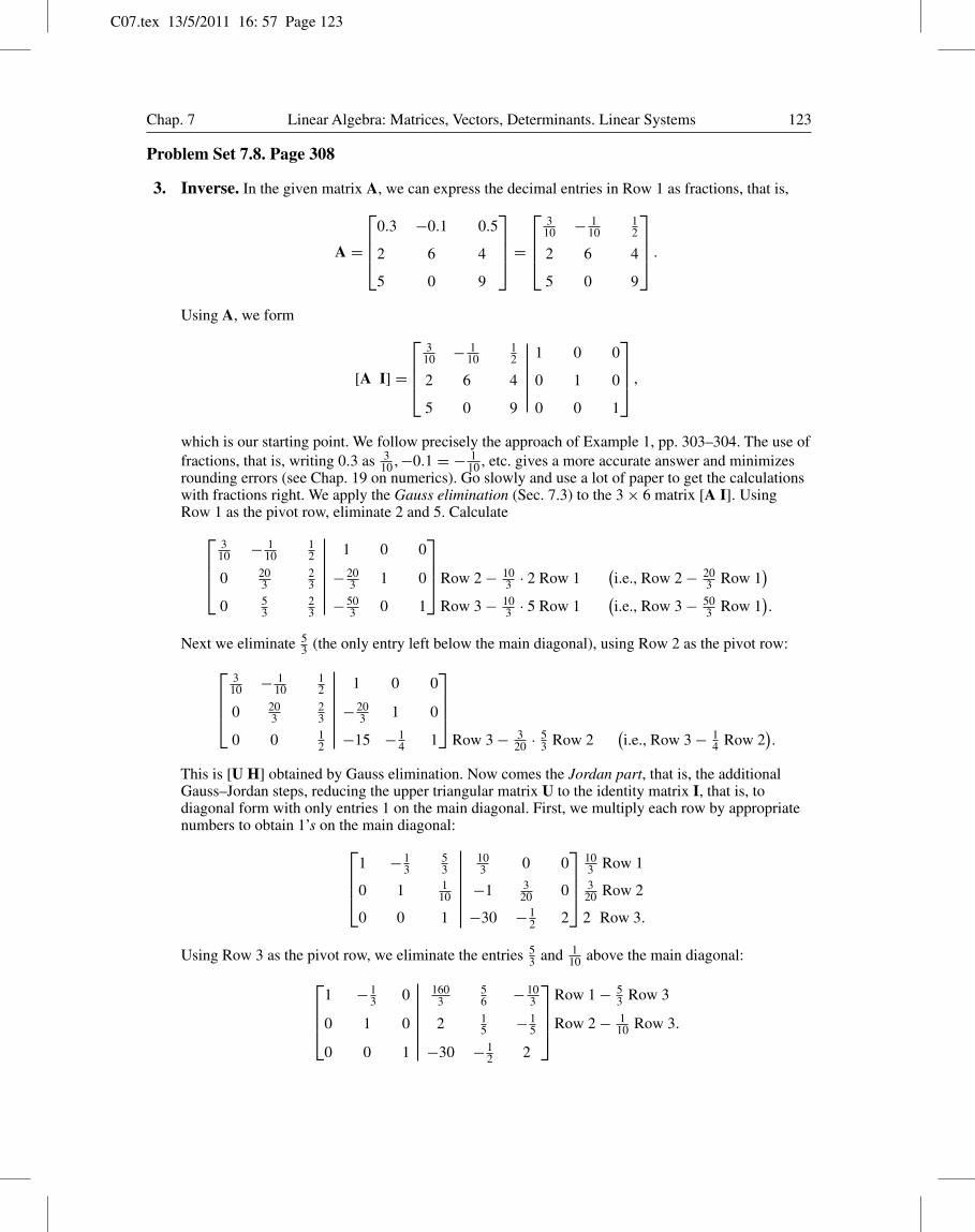
3. Inverse. In the given matrix A, we can express the decimal entries in Row 1 as fractions, that is,
A =
0.3 −0.1 0.5
2 6 4
5 0 9
=
3
10 − 110
12
2 6 4
5 0 9
.
Using A, we form
[A I] =
3
10 − 110
12
2 6 4
5 0 9
1 0 0
0 1 0
0 0 1
,
which is our starting point. We follow precisely the approach of Example 1, pp. 303–304. The use offractions, that is, writing 0.3 as 3
10 , −0.1 = − 110 , etc. gives a more accurate answer and minimizes
rounding errors (see Chap. 19 on numerics). Go slowly and use a lot of paper to get the calculationswith fractions right. We apply the Gauss elimination (Sec. 7.3) to the 3 × 6 matrix [A I]. UsingRow 1 as the pivot row, eliminate 2 and 5. Calculate
310 − 1
1012
0 203
23
0 53
23
1 0 0
−203 1 0
−503 0 1
Row 2 − 103 · 2 Row 1
(i.e., Row 2 − 20
3 Row 1)
Row 3 − 103 · 5 Row 1
(i.e., Row 3 − 50
3 Row 1).
Next we eliminate 53 (the only entry left below the main diagonal), using Row 2 as the pivot row:
310 − 1
1012
0 203
23
0 0 12
1 0 0
−203 1 0
−15 −14 1
Row 3 − 3
20 · 53 Row 2
(i.e., Row 3 − 1
4 Row 2).
This is [U H] obtained by Gauss elimination. Now comes the Jordan part, that is, the additionalGauss–Jordan steps, reducing the upper triangular matrix U to the identity matrix I, that is, todiagonal form with only entries 1 on the main diagonal. First, we multiply each row by appropriatenumbers to obtain 1’s on the main diagonal:
1 −13
53
0 1 110
0 0 1
103 0 0
−1 320 0
−30 −12 2
103 Row 13
20 Row 2
2 Row 3.
Using Row 3 as the pivot row, we eliminate the entries 53 and 1
10 above the main diagonal:1 −1
3 0
0 1 0
0 0 1
1603
56 −10
3
2 15 −1
5
−30 −12 2
Row 1 − 5
3 Row 3
Row 2 − 110 Row 3.
C07.tex 13/5/2011 16: 57 Page 124
124 Linear Algebra. Vector Calculus Part B
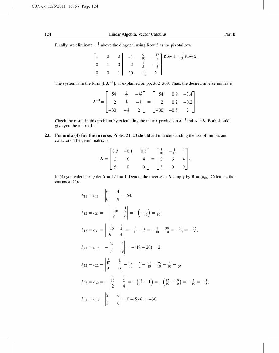
Finally, we eliminate −13 above the diagonal using Row 2 as the pivotal row:
1 0 0
0 1 0
0 0 1
54 910 −17
5
2 15 −1
5
−30 −12 2
Row 1 + 1
3 Row 2.
The system is in the form [I A−1], as explained on pp. 302–303. Thus, the desired inverse matrix is
A−1=
54 9
10 −175
2 15 −1
5
−30 −12 2
=
54 0.9 −3.4
2 0.2 −0.2
−30 −0.5 2
.
Check the result in this problem by calculating the matrix products AA−1and A−1A. Both shouldgive you the matrix I.
23. Formula (4) for the inverse. Probs. 21–23 should aid in understanding the use of minors andcofactors. The given matrix is
A =
0.3 −0.1 0.5
2 6 4
5 0 9
=
3
10 − 110
12
2 6 4
5 0 9
.
In (4) you calculate 1/ det A = 1/1 = 1. Denote the inverse of A simply by B = [bjk ]. Calculate theentries of (4):
b11 = c11 =∣∣∣∣∣6 4
0 9
∣∣∣∣∣ = 54,
b12 = c21 = −∣∣∣∣∣− 1
1012
0 9
∣∣∣∣∣ = −(− 9
10
)= 9
10 ,
b13 = c31 =∣∣∣∣∣− 1
1012
6 4
∣∣∣∣∣ = − 410 − 3 = − 4
10 − 3010 = −34
10 = −175 ,
b21 = c12 = −∣∣∣∣∣2 4
5 9
∣∣∣∣∣ = −(18 − 20) = 2,
b22 = c22 =∣∣∣∣∣ 3
1012
5 9
∣∣∣∣∣ = 2710 − 5
2 = 2710 − 25
10 = 210 = 1
5 ,
b23 = c32 = −∣∣∣∣∣ 3
1012
2 4
∣∣∣∣∣ = −(
1210 − 1
)= −
(1210 − 10
10
)= − 2
10 = −15 ,
b31 = c13 =∣∣∣∣∣2 6
5 0
∣∣∣∣∣ = 0 − 5 · 6 = −30,
C07.tex 13/5/2011 16: 57 Page 125
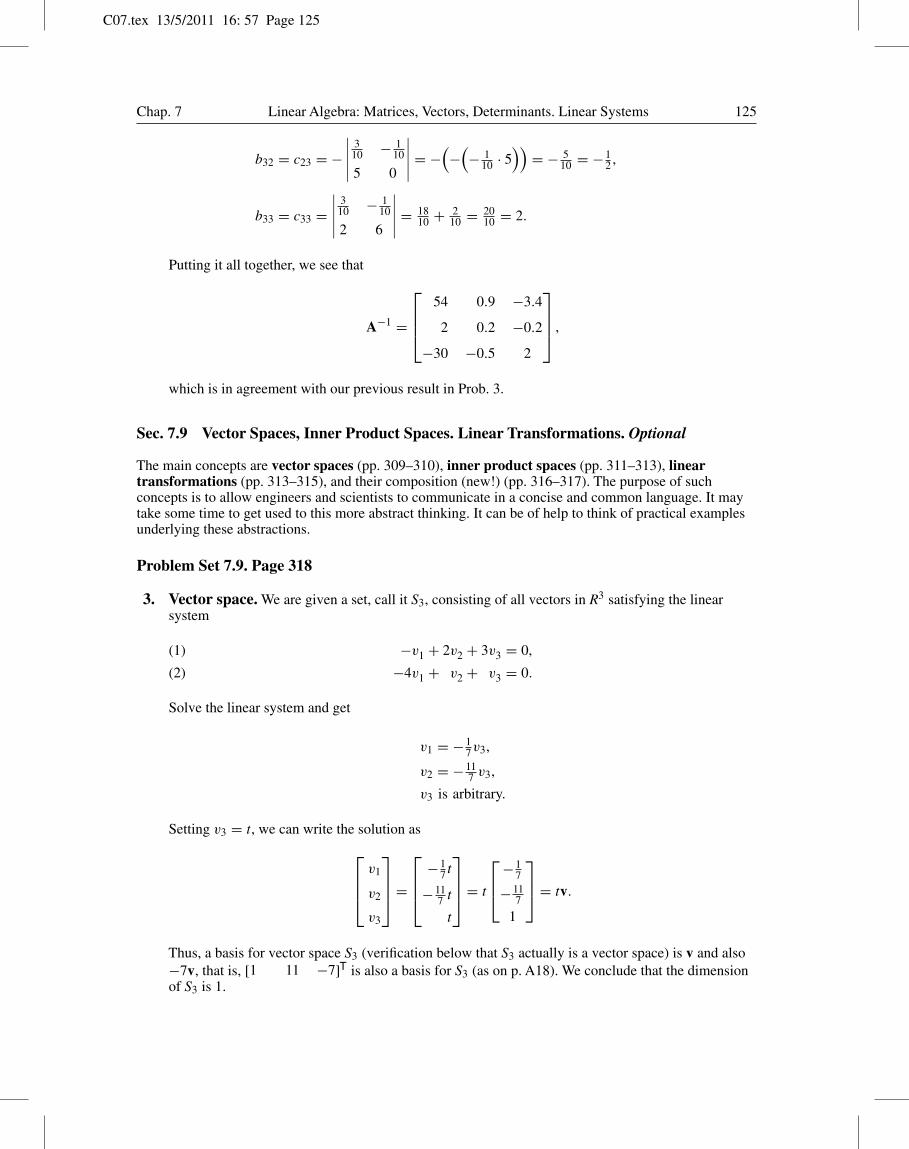
Chap. 7 Linear Algebra: Matrices, Vectors, Determinants. Linear Systems 125
b32 = c23 = −∣∣∣∣∣ 3
10 − 110
5 0
∣∣∣∣∣ = −(−
(− 1
10 · 5))
= − 510 = −1
2 ,
b33 = c33 =∣∣∣∣∣ 3
10 − 110
2 6
∣∣∣∣∣ = 1810 + 2
10 = 2010 = 2.
Putting it all together, we see that
A−1 =
54 0.9 −3.4
2 0.2 −0.2
−30 −0.5 2
,
which is in agreement with our previous result in Prob. 3.
Sec. 7.9 Vector Spaces, Inner Product Spaces. Linear Transformations. Optional
The main concepts are vector spaces (pp. 309–310), inner product spaces (pp. 311–313), lineartransformations (pp. 313–315), and their composition (new!) (pp. 316–317). The purpose of suchconcepts is to allow engineers and scientists to communicate in a concise and common language. It maytake some time to get used to this more abstract thinking. It can be of help to think of practical examplesunderlying these abstractions.
Problem Set 7.9. Page 318
3. Vector space. We are given a set, call it S3, consisting of all vectors in R3 satisfying the linearsystem
−v1 + 2v2 + 3v3 = 0,(1)
−4v1 + v2 + v3 = 0.(2)
Solve the linear system and get
v1 = −17v3,
v2 = −117 v3,
v3 is arbitrary.
Setting v3 = t, we can write the solution asv1
v2
v3
=
−1
7 t
−117 t
t
= t
−17
−117
1
= tv.
Thus, a basis for vector space S3 (verification below that S3 actually is a vector space) is v and also−7v, that is, [1 11 −7]T is also a basis for S3 (as on p. A18). We conclude that the dimensionof S3 is 1.
C07.tex 13/5/2011 16: 57 Page 126
126 Linear Algebra. Vector Calculus Part B
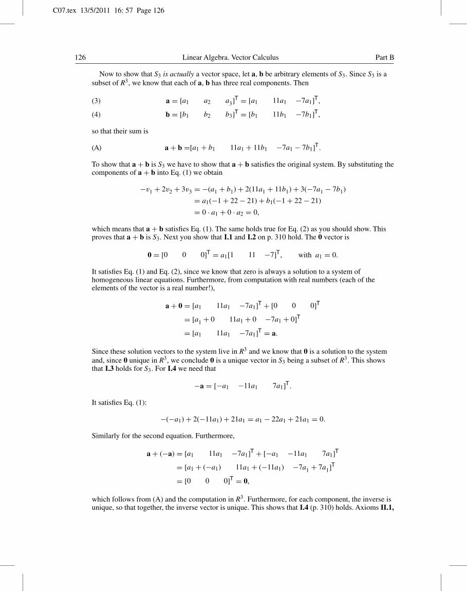
Now to show that S3 is actually a vector space, let a, b be arbitrary elements of S3. Since S3 is asubset of R3, we know that each of a, b has three real components. Then
a = [a1 a2 a3]T = [a1 11a1 −7a1]T,(3)
b = [b1 b2 b3]T = [b1 11b1 −7b1]T,(4)
so that their sum is
(A) a + b =[a1 + b1 11a1 + 11b1 −7a1 − 7b1]T.
To show that a + b is S3 we have to show that a + b satisfies the original system. By substituting thecomponents of a + b into Eq. (1) we obtain
−v1 + 2v2 + 3v3 = −(a1 + b1) + 2(11a1 + 11b1) + 3(−7a1 − 7b1)
= a1(−1 + 22 − 21) + b1(−1 + 22 − 21)
= 0 · a1 + 0 · a2 = 0,
which means that a + b satisfies Eq. (1). The same holds true for Eq. (2) as you should show. Thisproves that a + b is S3. Next you show that I.1 and I.2 on p. 310 hold. The 0 vector is
0 = [0 0 0]T = a1[1 11 −7]T, with a1 = 0.
It satisfies Eq. (1) and Eq. (2), since we know that zero is always a solution to a system ofhomogeneous linear equations. Furthermore, from computation with real numbers (each of theelements of the vector is a real number!),
a + 0 = [a1 11a1 −7a1]T + [0 0 0]T
= [a1 + 0 11a1 + 0 −7a1 + 0]T
= [a1 11a1 −7a1]T = a.
Since these solution vectors to the system live in R3 and we know that 0 is a solution to the systemand, since 0 unique in R3, we conclude 0 is a unique vector in S3 being a subset of R3. This showsthat I.3 holds for S3. For I.4 we need that
−a = [−a1 −11a1 7a1]T.
It satisfies Eq. (1):
−(−a1) + 2(−11a1) + 21a1 = a1 − 22a1 + 21a1 = 0.
Similarly for the second equation. Furthermore,
a + (−a) = [a1 11a1 −7a1]T + [−a1 −11a1 7a1]T
= [a1 + (−a1) 11a1 + (−11a1) −7a1 + 7a1]T
= [0 0 0]T = 0,
which follows from (A) and the computation in R3. Furthermore, for each component, the inverse isunique, so that together, the inverse vector is unique. This shows that I.4 (p. 310) holds. Axioms II.1,
C07.tex 13/5/2011 16: 57 Page 127
Chap. 7 Linear Algebra: Matrices, Vectors, Determinants. Linear Systems 127
II.2, III.3 are satisfied, as you should show. They hinge on the idea that if a satisfies Eq. (1) andEq. (2), so does ka for any real scalar k. To show II.4 we note that for
1a = 1[a1 a2 a3]T = 1[a1 11a1 −7a1]T
= [1a1 1 · 11a1 1 · (−7)a1]T = a,
so that II.4 is satisfied. After you have filled in all the indicated missing steps, you get a completeproof that S3 is indeed a vector space.
5. Not a vector space. From the problem description, we consider a set, call it S5, consisting ofpolynomials of the form (under the usual addition and scalar multiplication of polynomials)
(B) a0 + a1x + a2x2 + a3x3 + a4x4
with the added condition
(C) a0, a1, a2, a3, a4 � 0.
S5 is not a vector space. The problem lies in condition (C), which violates Axiom I.4. Indeed, choosesome coefficients not all zero, say, a0 = 1 and a4 = 7 (with the others zero). We obtain a polynomial1 + 7x4. It is clearly in S5. Its inverse is
(A1) −(1 + 7x4) = −1 − 7x4
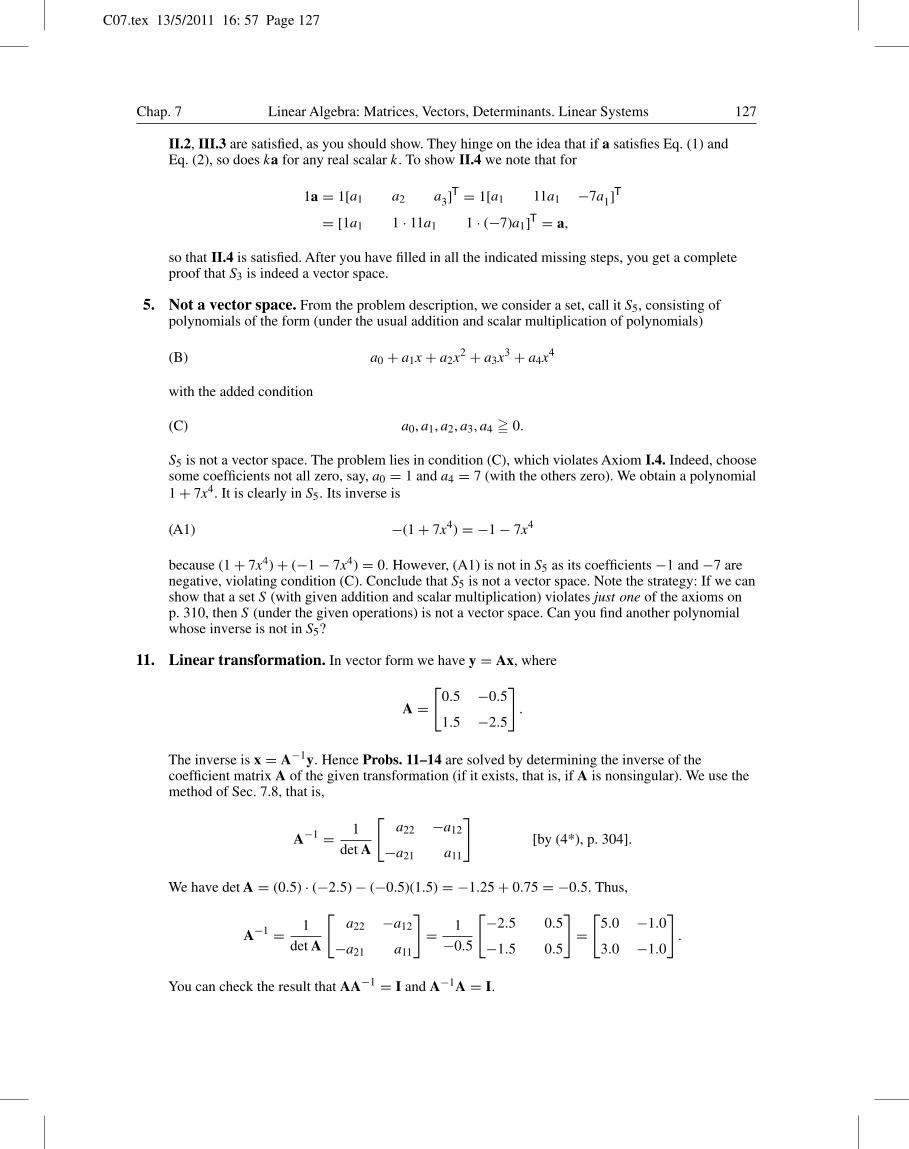
because (1 + 7x4) + (−1 − 7x4) = 0. However, (A1) is not in S5 as its coefficients −1 and −7 arenegative, violating condition (C). Conclude that S5 is not a vector space. Note the strategy: If we canshow that a set S (with given addition and scalar multiplication) violates just one of the axioms onp. 310, then S (under the given operations) is not a vector space. Can you find another polynomialwhose inverse is not in S5?
11. Linear transformation. In vector form we have y = Ax, where
A =[
0.5 −0.5
1.5 −2.5
].
The inverse is x = A−1y. Hence Probs. 11–14 are solved by determining the inverse of thecoefficient matrix A of the given transformation (if it exists, that is, if A is nonsingular). We use themethod of Sec. 7.8, that is,
A−1 = 1
det A
[a22 −a12
−a21 a11
][by (4*), p. 304].
We have det A = (0.5) · (−2.5) − (−0.5)(1.5) = −1.25 + 0.75 = −0.5. Thus,
A−1 = 1
det A
[a22 −a12
−a21 a11
]= 1
−0.5
[−2.5 0.5
−1.5 0.5
]=
[5.0 −1.0
3.0 −1.0
].
You can check the result that AA−1 = I and A−1A = I.
C07.tex 13/5/2011 16: 57 Page 128
128 Linear Algebra. Vector Calculus Part B
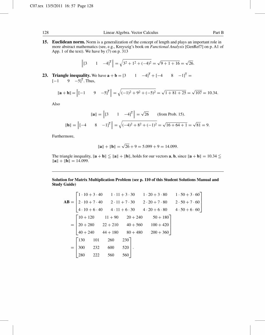
15. Euclidean norm. Norm is a generalization of the concept of length and plays an important role inmore abstract mathematics (see, e.g., Kreyszig’s book on Functional Analysis [GenRef7] on p. A1 ofApp. 1 of the text). We have by (7) on p. 313∥∥∥[3 1 −4]T
∥∥∥ =√
32 + 12 + (−4)2 = √9 + 1 + 16 = √
26.
23. Triangle inequality. We have a + b = [3 1 −4]T + [−4 8 −1]T =[−1 9 −5]T. Thus,
‖a + b‖ =∥∥∥[−1 9 −5]T
∥∥∥ =√
(−1)2 + 92 + (−5)2 = √1 + 81 + 25 = √
107 = 10.34.
Also
‖a‖ =∥∥∥[3 1 −4]T
∥∥∥ = √26 (from Prob. 15).
‖b‖ =∥∥∥[−4 8 −1]T
∥∥∥ =√
(−4)2 + 82 + (−1)2 = √16 + 64 + 1 = √
81 = 9.
Furthermore,
‖a‖ + ‖b‖ = √26 + 9 = 5.099 + 9 = 14.099.
The triangle inequality, ‖a + b‖ � ‖a‖ + ‖b‖, holds for our vectors a, b, since ‖a + b‖ = 10.34 �‖a‖ + ‖b‖ = 14.099.
Solution for Matrix Multiplication Problem (see p. 110 of this Student Solutions Manual andStudy Guide)
AB =
1 · 10 + 3 · 40 1 · 11 + 3 · 30 1 · 20 + 3 · 80 1 · 50 + 3 · 60
2 · 10 + 7 · 40 2 · 11 + 7 · 30 2 · 20 + 7 · 80 2 · 50 + 7 · 60
4 · 10 + 6 · 40 4 · 11 + 6 · 30 4 · 20 + 6 · 80 4 · 50 + 6 · 60
=
10 + 120 11 + 90 20 + 240 50 + 180
20 + 280 22 + 210 40 + 560 100 + 420
40 + 240 44 + 180 80 + 480 200 + 360
=
130 101 260 230
300 232 600 520
280 222 560 560
.