limits on eﬃcient computation in the physical world · 1 abstract limits on eﬃcient computation...

Limits on Efficient Computation in the Physical World

by

Scott Joel Aaronson

Bachelor of Science (Cornell University) 2000

A dissertation submitted in partial satisfaction of the

requirements for the degree of

Doctor of Philosophy

in

Computer Science

in the

GRADUATE DIVISION

of the

UNIVERSITY of CALIFORNIA, BERKELEY

Committee in charge:

Professor Umesh Vazirani, ChairProfessor Luca Trevisan

Professor K. Birgitta Whaley

Fall 2004

The dissertation of Scott Joel Aaronson is approved:

Chair Date

Date

Date

University of California, Berkeley

Fall 2004


Copyright 2004by

Scott Joel Aaronson

1

Abstract


by

Scott Joel AaronsonDoctor of Philosophy in Computer Science

University of California, Berkeley

Professor Umesh Vazirani, Chair

More than a speculative technology, quantum computing seems to challenge our most basicintuitions about how the physical world should behave. In this thesis I show that, whilesome intuitions from classical computer science must be jettisoned in the light of modernphysics, many others emerge nearly unscathed; and I use powerful tools from computationalcomplexity theory to help determine which are which.

In the first part of the thesis, I attack the common belief that quantum computingresembles classical exponential parallelism, by showing that quantum computers would faceserious limitations on a wider range of problems than was previously known. In partic-ular, any quantum algorithm that solves the collision problem—that of deciding whethera sequence of n integers is one-to-one or two-to-one—must query the sequence Ω

(n1/5

)

times. This resolves a question that was open for years; previously no lower bound betterthan constant was known. A corollary is that there is no “black-box” quantum algorithmto break cryptographic hash functions or solve the Graph Isomorphism problem in poly-nomial time. I also show that relative to an oracle, quantum computers could not solveNP-complete problems in polynomial time, even with the help of nonuniform “quantumadvice states”; and that any quantum algorithm needs Ω

(2n/4/n

)queries to find a local

minimum of a black-box function on the n-dimensional hypercube. Surprisingly, the latterresult also leads to new classical lower bounds for the local search problem. Finally, I givenew lower bounds on quantum one-way communication complexity, and on the quantumquery complexity of total Boolean functions and recursive Fourier sampling.

The second part of the thesis studies the relationship of the quantum computingmodel to physical reality. I first examine the arguments of Leonid Levin, Stephen Wol-fram, and others who believe quantum computing to be fundamentally impossible. I findtheir arguments unconvincing without a “Sure/Shor separator”—a criterion that separatesthe already-verified quantum states from those that appear in Shor’s factoring algorithm.I argue that such a separator should be based on a complexity classification of quantumstates, and go on to create such a classification. Next I ask what happens to the quantumcomputing model if we take into account that the speed of light is finite—and in particu-lar, whether Grover’s algorithm still yields a quadratic speedup for searching a database.Refuting a claim by Benioff, I show that the surprising answer is yes. Finally, I analyzehypothetical models of computation that go even beyond quantum computing. I show that

2

many such models would be as powerful as the complexity class PP, and use this fact togive a simple, quantum computing based proof that PP is closed under intersection. Onthe other hand, I also present one model—wherein we could sample the entire history ofa hidden variable—that appears to be more powerful than standard quantum computing,but only slightly so.

Professor Umesh VaziraniDissertation Committee Chair

iii

Contents

List of Figures vii

List of Tables viii

1 “Aren’t You Worried That Quantum Computing Won’t Pan Out?” 1

2 Overview 62.1 Limitations of Quantum Computers . . . . . . . . . . . . . . . . . . . . . . 7

2.1.1 The Collision Problem . . . . . . . . . . . . . . . . . . . . . . . . . . 82.1.2 Local Search . . . . . . . . . . . . . . . . . . . . . . . . . . . . . . . 92.1.3 Quantum Certificate Complexity . . . . . . . . . . . . . . . . . . . . 102.1.4 The Need to Uncompute . . . . . . . . . . . . . . . . . . . . . . . . . 112.1.5 Limitations of Quantum Advice . . . . . . . . . . . . . . . . . . . . . 11

2.2 Models and Reality . . . . . . . . . . . . . . . . . . . . . . . . . . . . . . . . 132.2.1 Skepticism of Quantum Computing . . . . . . . . . . . . . . . . . . . 132.2.2 Complexity Theory of Quantum States . . . . . . . . . . . . . . . . 132.2.3 Quantum Search of Spatial Regions . . . . . . . . . . . . . . . . . . 142.2.4 Quantum Computing and Postselection . . . . . . . . . . . . . . . . 152.2.5 The Power of History . . . . . . . . . . . . . . . . . . . . . . . . . . 16

3 Complexity Theory Cheat Sheet 183.1 The Complexity Zoo Junior . . . . . . . . . . . . . . . . . . . . . . . . . . . 193.2 Notation . . . . . . . . . . . . . . . . . . . . . . . . . . . . . . . . . . . . . . 203.3 Oracles . . . . . . . . . . . . . . . . . . . . . . . . . . . . . . . . . . . . . . 21

4 Quantum Computing Cheat Sheet 234.1 Quantum Computers: N Qubits . . . . . . . . . . . . . . . . . . . . . . . . 244.2 Further Concepts . . . . . . . . . . . . . . . . . . . . . . . . . . . . . . . . . 27

I Limitations of Quantum Computers 29

5 Introduction 305.1 The Quantum Black-Box Model . . . . . . . . . . . . . . . . . . . . . . . . . 315.2 Oracle Separations . . . . . . . . . . . . . . . . . . . . . . . . . . . . . . . . 32

iv

6 The Collision Problem 346.1 Motivation . . . . . . . . . . . . . . . . . . . . . . . . . . . . . . . . . . . . 36

6.1.1 Oracle Hardness Results . . . . . . . . . . . . . . . . . . . . . . . . . 366.1.2 Information Erasure . . . . . . . . . . . . . . . . . . . . . . . . . . . 36

6.2 Preliminaries . . . . . . . . . . . . . . . . . . . . . . . . . . . . . . . . . . . 376.3 Reduction to Bivariate Polynomial . . . . . . . . . . . . . . . . . . . . . . . 386.4 Lower Bound . . . . . . . . . . . . . . . . . . . . . . . . . . . . . . . . . . . 416.5 Set Comparison . . . . . . . . . . . . . . . . . . . . . . . . . . . . . . . . . . 436.6 Open Problems . . . . . . . . . . . . . . . . . . . . . . . . . . . . . . . . . . 46

7 Local Search 477.1 Motivation . . . . . . . . . . . . . . . . . . . . . . . . . . . . . . . . . . . . 497.2 Preliminaries . . . . . . . . . . . . . . . . . . . . . . . . . . . . . . . . . . . 517.3 Relational Adversary Method . . . . . . . . . . . . . . . . . . . . . . . . . . 527.4 Snakes . . . . . . . . . . . . . . . . . . . . . . . . . . . . . . . . . . . . . . . 577.5 Specific Graphs . . . . . . . . . . . . . . . . . . . . . . . . . . . . . . . . . . 60

7.5.1 Boolean Hypercube . . . . . . . . . . . . . . . . . . . . . . . . . . . 607.5.2 Constant-Dimensional Grid Graph . . . . . . . . . . . . . . . . . . . 64

8 Quantum Certificate Complexity 678.1 Summary of Results . . . . . . . . . . . . . . . . . . . . . . . . . . . . . . . 688.2 Related Work . . . . . . . . . . . . . . . . . . . . . . . . . . . . . . . . . . . 708.3 Characterization of Quantum Certificate Complexity . . . . . . . . . . . . . 708.4 Quantum Lower Bound for Total Functions . . . . . . . . . . . . . . . . . . 728.5 Asymptotic Gaps . . . . . . . . . . . . . . . . . . . . . . . . . . . . . . . . . 74

8.5.1 Local Separations . . . . . . . . . . . . . . . . . . . . . . . . . . . . . 768.5.2 Symmetric Partial Functions . . . . . . . . . . . . . . . . . . . . . . 77

8.6 Open Problems . . . . . . . . . . . . . . . . . . . . . . . . . . . . . . . . . . 78

9 The Need to Uncompute 799.1 Preliminaries . . . . . . . . . . . . . . . . . . . . . . . . . . . . . . . . . . . 819.2 Quantum Lower Bound . . . . . . . . . . . . . . . . . . . . . . . . . . . . . 829.3 Open Problems . . . . . . . . . . . . . . . . . . . . . . . . . . . . . . . . . . 87

10 Limitations of Quantum Advice 8810.1 Preliminaries . . . . . . . . . . . . . . . . . . . . . . . . . . . . . . . . . . . 91

10.1.1 Quantum Advice . . . . . . . . . . . . . . . . . . . . . . . . . . . . . 9210.1.2 The Almost As Good As New Lemma . . . . . . . . . . . . . . . . . 93

10.2 Simulating Quantum Messages . . . . . . . . . . . . . . . . . . . . . . . . . 9310.2.1 Simulating Quantum Advice . . . . . . . . . . . . . . . . . . . . . . 96

10.3 A Direct Product Theorem for Quantum Search . . . . . . . . . . . . . . . 9910.4 The Trace Distance Method . . . . . . . . . . . . . . . . . . . . . . . . . . . 103

10.4.1 Applications . . . . . . . . . . . . . . . . . . . . . . . . . . . . . . . 10610.5 Open Problems . . . . . . . . . . . . . . . . . . . . . . . . . . . . . . . . . . 110

v

11 Summary of Part I 112

II Models and Reality 114

12 Skepticism of Quantum Computing 11612.1 Bell Inequalities and Long-Range Threads . . . . . . . . . . . . . . . . . . . 119

13 Complexity Theory of Quantum States 12613.1 Sure/Shor Separators . . . . . . . . . . . . . . . . . . . . . . . . . . . . . . . 12713.2 Classifying Quantum States . . . . . . . . . . . . . . . . . . . . . . . . . . . 13013.3 Basic Results . . . . . . . . . . . . . . . . . . . . . . . . . . . . . . . . . . . 13513.4 Relations Among Quantum State Classes . . . . . . . . . . . . . . . . . . . 13813.5 Lower Bounds . . . . . . . . . . . . . . . . . . . . . . . . . . . . . . . . . . . 141

13.5.1 Subgroup States . . . . . . . . . . . . . . . . . . . . . . . . . . . . . 14213.5.2 Shor States . . . . . . . . . . . . . . . . . . . . . . . . . . . . . . . . 14613.5.3 Tree Size and Persistence of Entanglement . . . . . . . . . . . . . . . 148

13.6 Manifestly Orthogonal Tree Size . . . . . . . . . . . . . . . . . . . . . . . . 14913.7 Computing With Tree States . . . . . . . . . . . . . . . . . . . . . . . . . . 15413.8 The Experimental Situation . . . . . . . . . . . . . . . . . . . . . . . . . . . 15713.9 Conclusion and Open Problems . . . . . . . . . . . . . . . . . . . . . . . . . 160

14 Quantum Search of Spatial Regions 16214.1 Summary of Results . . . . . . . . . . . . . . . . . . . . . . . . . . . . . . . 16214.2 Related Work . . . . . . . . . . . . . . . . . . . . . . . . . . . . . . . . . . . 16414.3 The Physics of Databases . . . . . . . . . . . . . . . . . . . . . . . . . . . . 16514.4 The Model . . . . . . . . . . . . . . . . . . . . . . . . . . . . . . . . . . . . 167

14.4.1 Locality Criteria . . . . . . . . . . . . . . . . . . . . . . . . . . . . . 16814.5 General Bounds . . . . . . . . . . . . . . . . . . . . . . . . . . . . . . . . . . 16914.6 Search on Grids . . . . . . . . . . . . . . . . . . . . . . . . . . . . . . . . . . 173

14.6.1 Amplitude Amplification . . . . . . . . . . . . . . . . . . . . . . . . 17414.6.2 Dimension At Least 3 . . . . . . . . . . . . . . . . . . . . . . . . . . 17514.6.3 Dimension 2 . . . . . . . . . . . . . . . . . . . . . . . . . . . . . . . . 18014.6.4 Multiple Marked Items . . . . . . . . . . . . . . . . . . . . . . . . . . 18114.6.5 Unknown Number of Marked Items . . . . . . . . . . . . . . . . . . . 184

14.7 Search on Irregular Graphs . . . . . . . . . . . . . . . . . . . . . . . . . . . 18514.7.1 Bits Scattered on a Graph . . . . . . . . . . . . . . . . . . . . . . . . 189

14.8 Application to Disjointness . . . . . . . . . . . . . . . . . . . . . . . . . . . 19014.9 Open Problems . . . . . . . . . . . . . . . . . . . . . . . . . . . . . . . . . . 191

15 Quantum Computing and Postselection 19215.1 The Class PostBQP . . . . . . . . . . . . . . . . . . . . . . . . . . . . . . . . 19315.2 Fantasy Quantum Mechanics . . . . . . . . . . . . . . . . . . . . . . . . . . 19615.3 Open Problems . . . . . . . . . . . . . . . . . . . . . . . . . . . . . . . . . . 198

vi

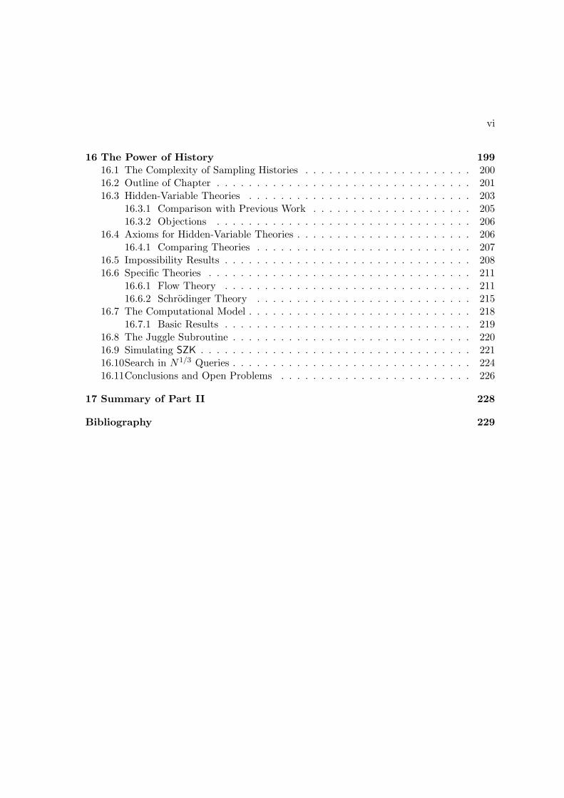
16 The Power of History 19916.1 The Complexity of Sampling Histories . . . . . . . . . . . . . . . . . . . . . 20016.2 Outline of Chapter . . . . . . . . . . . . . . . . . . . . . . . . . . . . . . . . 20116.3 Hidden-Variable Theories . . . . . . . . . . . . . . . . . . . . . . . . . . . . 203

16.3.1 Comparison with Previous Work . . . . . . . . . . . . . . . . . . . . 20516.3.2 Objections . . . . . . . . . . . . . . . . . . . . . . . . . . . . . . . . 206

16.4 Axioms for Hidden-Variable Theories . . . . . . . . . . . . . . . . . . . . . . 20616.4.1 Comparing Theories . . . . . . . . . . . . . . . . . . . . . . . . . . . 207

16.5 Impossibility Results . . . . . . . . . . . . . . . . . . . . . . . . . . . . . . . 20816.6 Specific Theories . . . . . . . . . . . . . . . . . . . . . . . . . . . . . . . . . 211

16.6.1 Flow Theory . . . . . . . . . . . . . . . . . . . . . . . . . . . . . . . 21116.6.2 Schrodinger Theory . . . . . . . . . . . . . . . . . . . . . . . . . . . 215

16.7 The Computational Model . . . . . . . . . . . . . . . . . . . . . . . . . . . . 21816.7.1 Basic Results . . . . . . . . . . . . . . . . . . . . . . . . . . . . . . . 219

16.8 The Juggle Subroutine . . . . . . . . . . . . . . . . . . . . . . . . . . . . . . 22016.9 Simulating SZK . . . . . . . . . . . . . . . . . . . . . . . . . . . . . . . . . . 22116.10Search in N1/3 Queries . . . . . . . . . . . . . . . . . . . . . . . . . . . . . . 22416.11Conclusions and Open Problems . . . . . . . . . . . . . . . . . . . . . . . . 226

17 Summary of Part II 228

Bibliography 229

vii

List of Figures

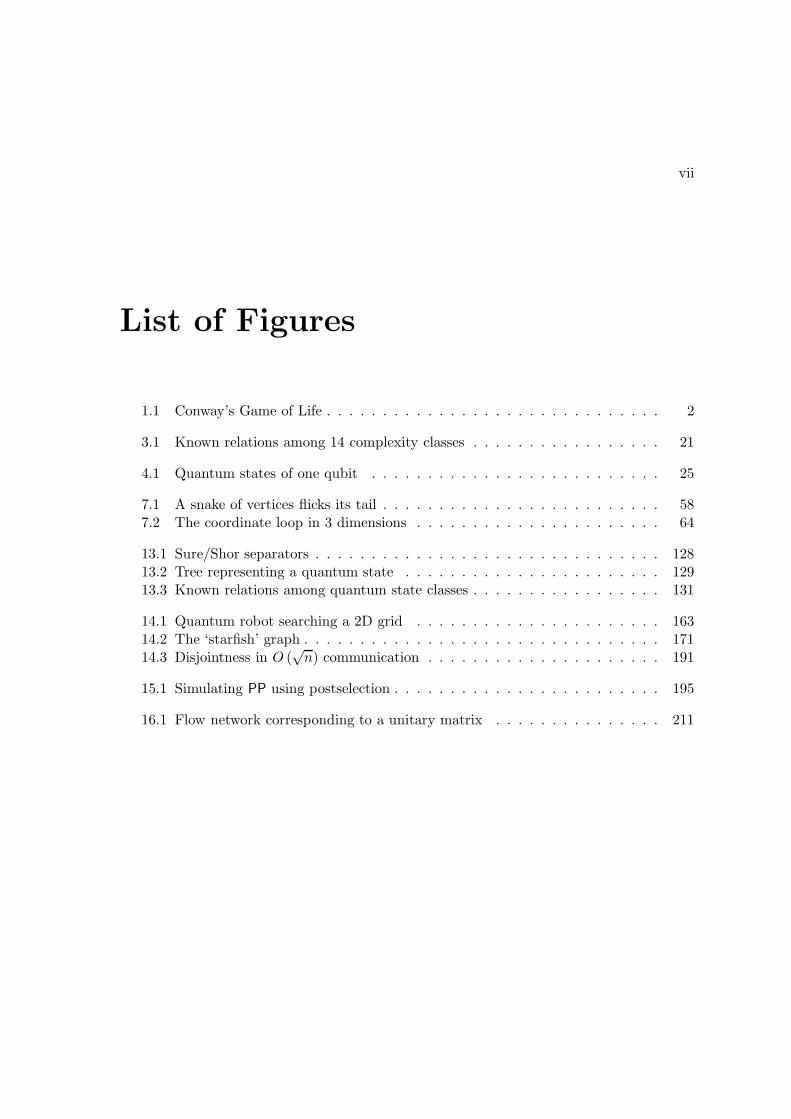
1.1 Conway’s Game of Life . . . . . . . . . . . . . . . . . . . . . . . . . . . . . . 2

3.1 Known relations among 14 complexity classes . . . . . . . . . . . . . . . . . 21

4.1 Quantum states of one qubit . . . . . . . . . . . . . . . . . . . . . . . . . . 25

7.1 A snake of vertices flicks its tail . . . . . . . . . . . . . . . . . . . . . . . . . 587.2 The coordinate loop in 3 dimensions . . . . . . . . . . . . . . . . . . . . . . 64

13.1 Sure/Shor separators . . . . . . . . . . . . . . . . . . . . . . . . . . . . . . . 12813.2 Tree representing a quantum state . . . . . . . . . . . . . . . . . . . . . . . 12913.3 Known relations among quantum state classes . . . . . . . . . . . . . . . . . 131

14.1 Quantum robot searching a 2D grid . . . . . . . . . . . . . . . . . . . . . . 16314.2 The ‘starfish’ graph . . . . . . . . . . . . . . . . . . . . . . . . . . . . . . . . 17114.3 Disjointness in O (

√n) communication . . . . . . . . . . . . . . . . . . . . . 191

15.1 Simulating PP using postselection . . . . . . . . . . . . . . . . . . . . . . . . 195

16.1 Flow network corresponding to a unitary matrix . . . . . . . . . . . . . . . 211

viii

List of Tables

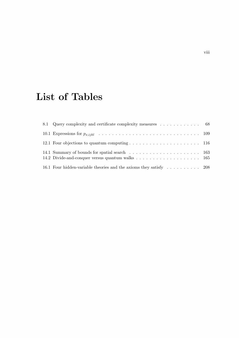
8.1 Query complexity and certificate complexity measures . . . . . . . . . . . . 68

10.1 Expressions for px,ijkl . . . . . . . . . . . . . . . . . . . . . . . . . . . . . . 109

12.1 Four objections to quantum computing . . . . . . . . . . . . . . . . . . . . . 116

14.1 Summary of bounds for spatial search . . . . . . . . . . . . . . . . . . . . . 16314.2 Divide-and-conquer versus quantum walks . . . . . . . . . . . . . . . . . . . 165

16.1 Four hidden-variable theories and the axioms they satisfy . . . . . . . . . . 208

ix

Acknowledgements

My adviser, Umesh Vazirani, once said that he admires the quantum adiabatic algorithmbecause, like a great squash player, it achieves its goal while moving as little as it can getaway with. Throughout my four years at Berkeley, I saw Umesh inculcate by example his“adiabatic” philosophy of life: a philosophy about which papers are worth reading, whichdeadlines worth meeting, and which research problems worth a fight to the finish. Above all,the concept of “beyond hope” does not exist in this philosophy, except possibly in regardto computational problems. My debt to Umesh for his expert scientific guidance, wiseprofessional counsel, and generous support is obvious and beyond my ability to embellish.My hope is that I graduate from Berkeley a more adiabatic person than when I came.

Admittedly, if the push to finish this thesis could be called adiabatic, then thespectral gap was exponentially small. As I struggled to make the deadline, I relied on thehelp of David Molnar, who generously agreed to file the thesis in Berkeley while I remained inPrinceton; and my committee—consisting of Umesh, Luca Trevisan, and Birgitta Whaley—which met procrastination with flexibility.

Silly as it sounds, a principal reason I came to Berkeley was to breathe the same airthat led Andris Ambainis to write his epochal paper “Quantum lower bounds by quantumarguments.” Whether or not the air in 587 Soda did me any good, Part I of the thesis isessentially a 150-page tribute to Andris—a colleague whose unique combination of geniusand humility fills everyone who knows him with awe.

The direction of my research owes a great deal as well to Ronald de Wolf, whoperiodically emerges from his hermit cave to challenge non-rigorous statements, eat dubbelzout, or lament American ignorance. While I can see eye-to-eye with Ronald about (say)the D (f) versus bs (f)2 problem, I still feel that Andrei Tarkovsky’s Solaris would benefitimmensely from a car chase.

For better or worse, my conception of what a thesis should be was influenced byDave Bacon, quantum computing’s elder clown, who entitled the first chapter of his own451-page behemoth “Philosonomicon.” I’m also indebted to Chris Fuchs and his samizdat,for the idea that a document about quantum mechanics more than 400 pages long can beworth reading most of the way through.

I began working on the best-known result in this thesis, the quantum lower boundfor the collision problem, during an unforgettable summer at Caltech. Leonard Schul-man and Ashwin Nayak listened patiently to one farfetched idea after another, while JohnPreskill’s weekly group meetings helped to ensure that the mysteries of quantum mechanics,which inspired me to tackle the problem in the first place, were never far from my mind.Besides Leonard, Ashwin, and John, I’m grateful to Ann Harvey for putting up with thegrowing mess in my office. For the record, I never once slept in the office; the bedsheetwas strictly for doing math on the floor.

I created the infamous Complexity Zoo web site during a summer at CWI inAmsterdam, a visit enlivened by the presence of Harry Buhrman, Hein Rohrig, VolkerNannen, Hartmut Klauck, and Troy Lee. That summer I also had memorable conversationswith David Deutsch and Stephen Wolfram. Chapters 7, 13, and 16 partly came into beingduring a semester at the Hebrew University in Jerusalem, a city where “Aaron’s sons” werealready obsessing about cubits three thousand years ago. I thank Avi Wigderson, Dorit

x

Aharonov, Michael Ben-Or, Amnon Ta-Shma, and Michael Mallin for making that semestera fruitful and enjoyable one. I also thank Avi for pointing me to the then-unpublishedresults of Ran Raz on which Chapter 13 is based, and Ran for sharing those results.

A significant chunk of the thesis was written or revised over two summers at thePerimeter Institute for Theoretical Physics in Waterloo. I thank Daniel Gottesman, LeeSmolin, and Ray Laflamme for welcoming a physics doofus to their institute, someone whothinks the string theory versus loop quantum gravity debate should be resolved by loopingover all possible strings. From Marie Ericsson, Rob Spekkens, and Anthony ValentiniI learned that theoretical physicists have a better social life than theoretical computerscientists, while from Dan Christensen I learned that complexity and quantum gravity hadbetter wait before going steady.

Several ideas were hatched or incubated during the yearly QIP conferences; work-shops in Toronto, Banff, and Leiden; and visits to MIT, Los Alamos, and IBM Almaden.I’m grateful to Howard Barnum, Andrew Childs, Elham Kashefi, Barbara Terhal, JohnWatrous, and many others for productive exchanges on those occasions.

Back in Berkeley, people who enriched my grad-school experience include NehaDave, Julia Kempe, Simone Severini, Lawrence Ip, Allison Coates, David Molnar, Kris Hil-drum, Miriam Walker, and Shelly Rosenfeld. Alex Fabrikant and Boriska Toth are forgivenfor the cruel caricature that they attached to my dissertation talk announcement, providedthey don’t try anything like that ever again. The results on one-way communication inChapter 10 benefited greatly from conversations with Oded Regev and Iordanis Kerenidis,while Andrej Bogdanov kindly supplied the explicit erasure code for Chapter 13. I wroteChapter 7 to answer a question of Christos Papadimitriou.

I did take some actual . . . courses at Berkeley, and I’m grateful to John Kubiatow-icz, Stuart Russell, Guido Bacciagaluppi, Richard Karp, and Satish Rao for not failing mein theirs. Ironically, the course that most directly influenced this thesis was Tom Farber’smagnificent short fiction workshop. A story I wrote for that workshop dealt with the prob-lem of transtemporal identity, which got me thinking about hidden-variable interpretationsof quantum mechanics, which led eventually to the collision lower bound. No one seems tobelieve me, but it’s true.

The students who took my “Physics, Philosophy, Pizza” course remain one of mygreatest inspirations. Though they were mainly undergraduates with liberal arts back-grounds, they took nothing I said about special relativity or Godel’s Theorem on faith. IfI have any confidence today in my teaching abilities; if I think it possible for students toshow up to class, and to participate eagerly, without the usual carrot-and-stick of gradesand exams; or if I find certain questions, such as how a superposition over exponentiallymany ‘could-have-beens’ can collapse to an ‘is,’ too vertiginous to be pondered only bynerds like me, then those pizza-eating students are the reason.

Now comes the part devoted to the mist-enshrouded pre-Berkeley years. Myinitiation into the wild world of quantum computing research took place over three summerinternships at Bell Labs: the first with Eric Grosse, the second with Lov Grover, and thethird with Rob Pike. I thank all three of them for encouraging me to pursue my interests,even if the payoff was remote and, in Eric’s case, not even related to why I was hired.Needless to say, I take no responsibility for the subsequent crash of Lucent’s stock.

xi

As an undergraduate at Cornell, I was younger than my classmates, invisible tomany of the researchers I admired, and profoundly unsure of whether I belonged there orhad any future in science. What made the difference was the unwavering support of oneprofessor, Bart Selman. Busy as he was, Bart listened to my harebrained ideas aboutgenetic algorithms for SAT or quantum chess-playing, invited me to give talks, guided meto the right graduate programs, and generally treated me like a future colleague. Asa result, his conviction that I could succeed at research gradually became my convictiontoo. Outside of research, Christine Chung, Fion Luo, and my Telluride roommate JasonStockmann helped to warm the Ithaca winters, Lydia Fakundiny taught me what an essayis, and Jerry Abrams provided a much-needed boost.

Turning the clock back further, my earliest research foray was a paper on hypertextorganization, written when I was fifteen and spending the year at Clarkson University’sunique Clarkson School program. Christopher Lynch generously agreed to advise theproject, and offered invaluable help as I clumsily learned how to write a C program, provea problem NP-hard, and conduct a user experiment (one skill I’ve never needed again!). Iwas elated to be trading ideas with a wise and experienced researcher, only months after I’descaped from the prison-house of high school. Later, the same week the rejection letterswere arriving from colleges, I learned that my first paper had been accepted to SIGIR,the main information retrieval conference. I was filled with boundless gratitude towardthe entire scientific community—for struggling, against the warp of human nature, to judgeideas rather than the personal backgrounds of their authors. Eight years later, my gratitudeand amazement are undiminished.

Above all, I thank Alex Halderman for a friendship that’s spanned twelve yearsand thousands of miles, remaining as strong today as it was amidst the Intellectualis minimiof Newtown Junior High School; my brother David for believing in me, and for making meprouder than he realizes by doing all the things I didn’t; and my parents for twenty-threeyears of harping, kvelling, chicken noodle soup, and never doubting for a Planck time thatI’d live up to my potential—even when I couldn’t, and can’t, share their certainty.

1

Chapter 1

“Aren’t You Worried ThatQuantum Computing Won’t PanOut?”

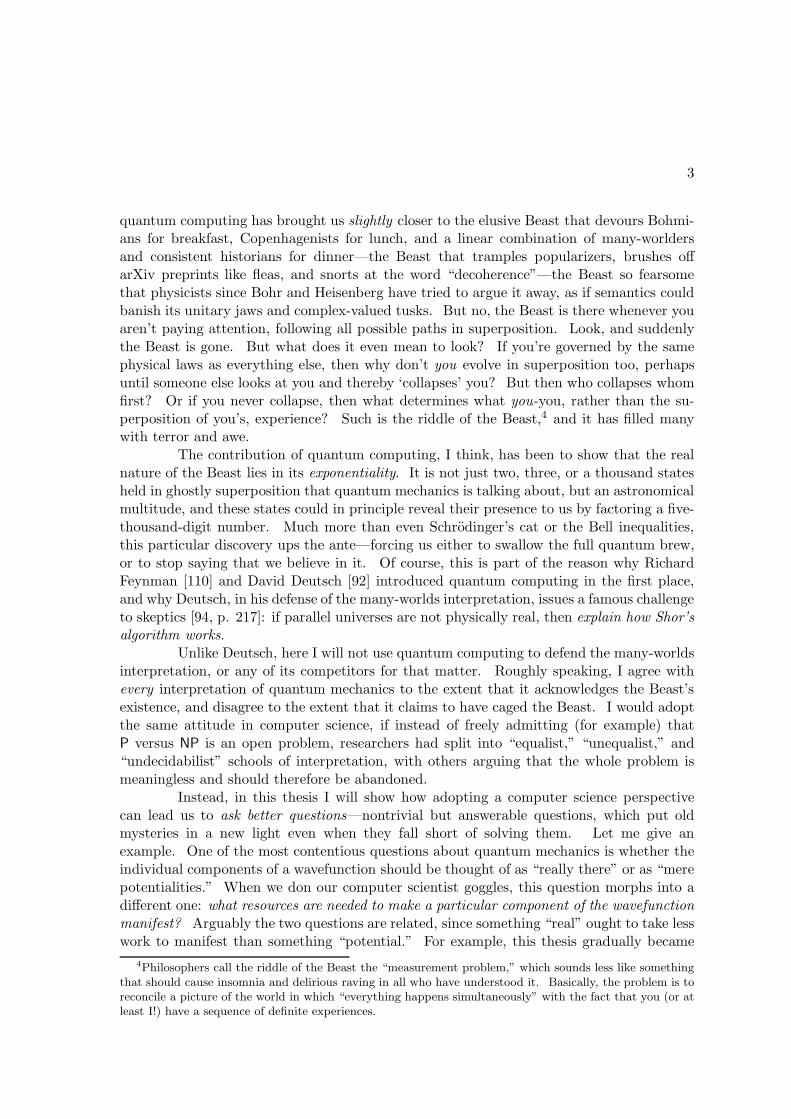
For a century now, physicists have been telling us strange things: about twinswho age at different rates, particles that look different when rotated 360, a force that istransmitted by gravitons but is also the curvature of spacetime, a negative-energy electronsea that pervades empty space, and strangest of all, “probability waves” that produce fringeson a screen when you don’t look and don’t when you do. Yet ever since I learned to program,I suspected that such things were all “implementation details” in the source code of Nature,their study only marginally relevant to forming an accurate picture of reality. Physicists,I thought, would eventually realize that the state of the universe can be represented bya finite string of bits. These bits would be the “pixels” of space, creating the illusion ofcontinuity on a large scale much as a computer screen does. As time passed, the bitswould be updated according to simple rules. The specific form of these rules was of nogreat consequence—since according to the Extended Church-Turing Thesis, any sufficientlycomplicated rules could simulate any other rules with reasonable efficiency.1 So apart frompractical considerations, why worry about Maxwell’s equations, or Lorentz invariance, oreven mass and energy, if the most fundamental aspects of our universe already occur inConway’s Game of Life (see Figure 1.1)?

Then I heard about Shor’s algorithm [221] for factoring integers in polynomial timeon a quantum computer. Then as now, many people saw quantum computing as at best aspeculative diversion from the “real work” of computer science. Why devote one’s researchcareer to a type of computer that might never see application within one’s lifetime, thatfaces daunting practical obstacles such as decoherence, and whose most publicized successto date has been the confirmation that, with high probability, 15 = 3× 5 [234]? Ironically,I might have agreed with this view, had I not taken the Extended Church-Turing Thesisso seriously as a claim about reality. For Shor’s algorithm forces us to accept that, under

1Here “extended” refers to the efficiency requirement, which was not mentioned in the original Church-Turing Thesis. Also, I am simply using the standard terminology, sidestepping the issue of whether Churchand Turing themselves intended to make a claim about physical reality.

2

Figure 1.1: In Conway’s Game of Life, each cell of a 2D square grid becomes ‘dead’ or‘alive’ based on how many of its eight neighbors were alive in the previous time step. Asimple rule applied iteratively leads to complex, unpredictable behavior. In what ways isour physical world similar to Conway’s, and in what ways is it different?

widely-believed assumptions, that Thesis conflicts with the experimentally-tested rules ofquantum mechanics as we currently understand them. Either the Extended Church-TuringThesis is false, or quantum mechanics must be modified, or the factoring problem is solvablein classical polynomial time. All three possibilities seem like wild, crackpot speculations—but at least one of them is true!

The above conundrum is what underlies my interest in quantum computing, farmore than any possible application. Part of the reason is that I am neither greedy, nefarious,nor number-theoretically curious enough ever to have hungered for the factors of a 600-digitinteger. I do think that quantum computers would have benign uses, the most importantone being the simulation of quantum physics and chemistry.2 Also, as transistors approachthe atomic scale, ideas from quantum computing are likely to become pertinent even forclassical computer design. But none of this quickens my pulse.

For me, quantum computing matters because it combines two of the great myster-ies bequeathed to us by the twentieth century: the nature of quantum mechanics, and theultimate limits of computation. It would be astonishing if such an elemental connectionbetween these mysteries shed no new light on either of them. And indeed, there is alreadya growing list of examples [9, 22, 153]—we will see several of them in this thesis—in whichideas from quantum computing have led to new results about classical computation. Thisshould not be surprising: after all, many celebrated results in computer science involveonly deterministic computation, yet it is hard to imagine how anyone could have provedthem had computer scientists not long ago “taken randomness aboard.”3 Likewise, takingquantum mechanics aboard could lead to a new, more general perspective from which torevisit the central questions of computational complexity theory.

The other direction, though, is the one that intrigues me even more. In my view,

2Followed closely by Recursive Fourier Sampling, parity in n/2 queries, and efficiently deciding whethera graph is a scorpion.

3A few examples are primality testing in P [17], undirected connectivity in L [204], and inapproximabilityof 3-SAT unless P = NP [226].

3

quantum computing has brought us slightly closer to the elusive Beast that devours Bohmi-ans for breakfast, Copenhagenists for lunch, and a linear combination of many-worldersand consistent historians for dinner—the Beast that tramples popularizers, brushes offarXiv preprints like fleas, and snorts at the word “decoherence”—the Beast so fearsomethat physicists since Bohr and Heisenberg have tried to argue it away, as if semantics couldbanish its unitary jaws and complex-valued tusks. But no, the Beast is there whenever youaren’t paying attention, following all possible paths in superposition. Look, and suddenlythe Beast is gone. But what does it even mean to look? If you’re governed by the samephysical laws as everything else, then why don’t you evolve in superposition too, perhapsuntil someone else looks at you and thereby ‘collapses’ you? But then who collapses whomfirst? Or if you never collapse, then what determines what you-you, rather than the su-perposition of you’s, experience? Such is the riddle of the Beast,4 and it has filled manywith terror and awe.

The contribution of quantum computing, I think, has been to show that the realnature of the Beast lies in its exponentiality. It is not just two, three, or a thousand statesheld in ghostly superposition that quantum mechanics is talking about, but an astronomicalmultitude, and these states could in principle reveal their presence to us by factoring a five-thousand-digit number. Much more than even Schrodinger’s cat or the Bell inequalities,this particular discovery ups the ante—forcing us either to swallow the full quantum brew,or to stop saying that we believe in it. Of course, this is part of the reason why RichardFeynman [110] and David Deutsch [92] introduced quantum computing in the first place,and why Deutsch, in his defense of the many-worlds interpretation, issues a famous challengeto skeptics [94, p. 217]: if parallel universes are not physically real, then explain how Shor’salgorithm works.

Unlike Deutsch, here I will not use quantum computing to defend the many-worldsinterpretation, or any of its competitors for that matter. Roughly speaking, I agree withevery interpretation of quantum mechanics to the extent that it acknowledges the Beast’sexistence, and disagree to the extent that it claims to have caged the Beast. I would adoptthe same attitude in computer science, if instead of freely admitting (for example) thatP versus NP is an open problem, researchers had split into “equalist,” “unequalist,” and“undecidabilist” schools of interpretation, with others arguing that the whole problem ismeaningless and should therefore be abandoned.

Instead, in this thesis I will show how adopting a computer science perspectivecan lead us to ask better questions—nontrivial but answerable questions, which put oldmysteries in a new light even when they fall short of solving them. Let me give anexample. One of the most contentious questions about quantum mechanics is whether theindividual components of a wavefunction should be thought of as “really there” or as “merepotentialities.” When we don our computer scientist goggles, this question morphs into adifferent one: what resources are needed to make a particular component of the wavefunctionmanifest? Arguably the two questions are related, since something “real” ought to take lesswork to manifest than something “potential.” For example, this thesis gradually became

4Philosophers call the riddle of the Beast the “measurement problem,” which sounds less like somethingthat should cause insomnia and delirious raving in all who have understood it. Basically, the problem is toreconcile a picture of the world in which “everything happens simultaneously” with the fact that you (or atleast I!) have a sequence of definite experiences.

4

more real as less of it remained to be written.Concretely, suppose our wavefunction has 2n components, all with equal ampli-

tude. Suppose also that we have a procedure to recognize a particular component x (i.e.,a function f such that f (x) = 1 and f (y) = 0 for all y 6= x). Then how often must weapply this procedure before we make x manifest; that is, observable with probability closeto 1? Bennett, Bernstein, Brassard, and Vazirani [51] showed that ∼ 2n/2 applications arenecessary, even if f can be applied to all 2n components in superposition. Later Grover[141] showed that ∼ 2n/2 applications are also sufficient. So if we imagine a spectrumwith “really there” (1 application) on one end, and “mere potentiality” (∼ 2n applications)on the other, then we have landed somewhere in between: closer to the “real” end on anabsolute scale, but closer to the “potential” end on the polynomial versus exponential scalethat is more natural for computer science.

Of course, we should be wary of drawing grand conclusions from a single datapoint. So in this thesis, I will imagine a hypothetical resident of Conway’s Game of Life,who arrives in our physical universe on a computational complexity safari—wanting toknow exactly which intuitions to keep and which to discard regarding the limits of efficientcomputation. Many popular science writers would tell our visitor to throw all classicalintuitions out the window, while quantum computing skeptics would urge retaining themall. These positions are actually two sides of the same coin, since the belief that a quantumcomputer would necessitate the first is what generally leads to the second. I will show,however, that neither position is justified. Based on what we know today, there really is aBeast, but it usually conceals its exponential underbelly.

I’ll provide only one example from the thesis here; the rest are summarized inChapter 2. Suppose we are given a procedure that computes a two-to-one function f ,and want to find distinct inputs x and y such that f (x) = f (y). In this case, by simplypreparing a uniform superposition over all inputs to f , applying the procedure, and thenmeasuring its result, we can produce a state of the form (|x〉 + |y〉) /

√2, for some x and y

such that f (x) = f (y). The only problem is that if we measure this state, then we seeeither x or y, but not both. The task, in other words, is no longer to find a needle ina haystack, but just to find two needles in an otherwise empty barn! Nevertheless, thecollision lower bound in Chapter 6 will show that, if there are 2n inputs to f , then anyquantum algorithm for this problem must apply the procedure for f at least ∼ 2n/5 times.Omitting technical details, this lower bound can be interpreted in at least seven ways:

(1) Quantum computers need exponential time even to compute certain global propertiesof a function, not just local properties such as whether there is an x with f (x) = 1.

(2) Simon’s algorithm [222], and the period-finding core of Shor’s algorithm [221], cannotbe generalized to functions with no periodicity or other special structure.

(3) Any “brute-force” quantum algorithm needs exponential time, not just for NP-completeproblems, but for many structured problems such as Graph Isomorphism, approxi-mating the shortest vector in a lattice, and finding collisions in cryptographic hashfunctions.

5

(4) It is unlikely that all problems having “statistical zero-knowledge proofs” can beefficiently solved on a quantum computer.

(5) Within the setting of a collision algorithm, the components |x〉 and |y〉 in the state(|x〉 + |y〉) /

√2 should be thought of as more “potentially” than “actually” there, it

being impossible to extract information about both of them in a reasonable amountof time.

(6) The ability to map |x〉 to |f (x)〉, “uncomputing” x in the process, can be exponentiallymore powerful than the ability to map |x〉 to |x〉 |f (x)〉.

(7) In hidden-variable interpretations of quantum mechanics, the ability to sample the en-tire history of a hidden variable would yield even more power than standard quantumcomputing.

Interpretations (5), (6), and (7) are examples of what I mean by putting oldmysteries in a new light. We are not brought face-to-face with the Beast, but at least wehave fresh footprints and droppings.

Well then. Am I worried that quantum computing won’t pan out? My usualanswer is that I’d be thrilled to know it will never pan out, since this would entail thediscovery of a lifetime, that quantum mechanics is false. But this is not what the questionerhas in mind. What if quantum mechanics holds up, but building a useful quantum computerturns out to be so difficult and expensive that the world ends before anyone succeeds? Thequestioner is usually a classical theoretical computer scientist, someone who is not known toworry excessively that the world will end before log logn exceeds 10. Still, it would be niceto see nontrivial quantum computers in my lifetime, and while I’m cautiously optimistic,I’ll admit to being slightly worried that I won’t. But when faced with the evidence thatone was born into a universe profoundly unlike Conway’s—indeed, that one is living one’slife on the back of a mysterious, exponential Beast comprising everything that ever couldhave happened—what is one to do? “Move right along. . . nothing to see here. . . ”

6

Chapter 2

Overview

“Let a computer smear—with the right kind of quantum randomness—andyou create, in effect, a ‘parallel’ machine with an astronomical number of pro-cessors . . . All you have to do is be sure that when you collapse the system,you choose the version that happened to find the needle in the mathematicalhaystack.”

—From Quarantine [105], a 1992 science-fiction novel by Greg Egan

Many of the deepest discoveries of science are limitations: for example, no su-perluminal signalling, no perpetual-motion machines, and no complete axiomatization forarithmetic. This thesis is broadly concerned with limitations on what can efficiently becomputed in the physical world. The word “quantum” is absent from the title, in orderto emphasize that the focus on quantum computing is not an arbitrary choice, but ratheran inevitable result of taking our current physical theories seriously. The technical con-tributions of the thesis are divided into two parts, according to whether they accept thequantum computing model as given and study its fundamental limitations; or question,defend, or go beyond that model in some way. Before launching into a detailed overviewof the contributions, let me make some preliminary remarks.

Since the early twentieth century, two communities—physicists1 and computerscientists—have been asking some of the deepest questions ever asked in almost total in-tellectual isolation from each other. The great joy of quantum computing research is thatit brings these communities together. The trouble was initially that, although each com-munity would nod politely during the other’s talks, eventually it would come out that thephysicists thought NP stood for “Non Polynomial,” and the computer scientists had noidea what a Hamiltonian was. Thankfully, the situation has improved a lot—but my hopeis that it improves further still, to the point where computer scientists have internalizedthe problems faced by physics and vice versa. For this reason, I have worked hard tomake the thesis as accessible as possible to both communities. Thus, Chapter 3 providesa “complexity theory cheat sheet” that defines NP, P/poly, AM, and other computationalcomplexity classes that appear in the thesis; and that explains oracles and other important

1As in Saul Steinberg’s famous New Yorker world map, in which 9th Avenue and the Hudson River takeup more space than Japan and China, from my perspective chemists, engineers, and even mathematicianswho know what a gauge field is are all “physicists.”

7

concepts. Then Chapter 4 presents the quantum model of computation with no referenceto the underlying physics, before moving on to fancier notions such as density matrices,trace distance, and separability. Neither chapter is a rigorous introduction to its subject;for that there are fine textbooks—such as Papadimitriou’s Computational Complexity [190]and Nielsen and Chuang’s Quantum Computation and Quantum Information [184]—as wellas course lecture notes available on the web. Depending on your background, you mightwant to skip to Chapters 3 or 4 before continuing any further, or you might want to skippast these chapters entirely.

Even the most irredeemably classical reader should take heart: of the 103 proofsin the thesis, 66 do not contain a single ket symbol.2 Many of the proofs can be understoodby simply accepting certain facts about quantum computing on faith, such as Ambainis’s3

adversary theorem [27] or Beals et al.’s polynomial lemma [45]. On the other hand, one doesrun the risk that after one understands the proofs, ket symbols will seem less frighteningthan before.

The results in the thesis have all previously appeared in published papers orpreprints [1, 2, 4, 5, 7, 8, 9, 10, 11, 13], with the exception of the quantum computingbased proof that PP is closed under intersection in Chapter 15. I thank Andris Ambainisfor allowing me to include our joint results from [13] on quantum search of spatial regions.Results of mine that do not appear in the thesis include those on Boolean function queryproperties [3], stabilizer circuits [14] (joint work with Daniel Gottesman), and agreementcomplexity [6].

In writing the thesis, one of the toughest choices I faced was whether to refer tomyself as ‘I’ or ‘we.’ Sometimes a personal voice seemed more appropriate, and sometimesthe Voice of Scientific Truth, but I wanted to be consistent. Readers can decide whether Ichose humbly or arrogantly.

2.1 Limitations of Quantum Computers

Part I studies the fundamental limitations of quantum computers within the usual modelfor them. With the exception of Chapter 10 on quantum advice, the contributions of PartI all deal with black-box or query complexity, meaning that one counts only the number ofqueries to an “oracle,” not the number of computational steps. Of course, the queries canbe made in quantum superposition. In Chapter 5, I explain the quantum black-box model,then offer a detailed justification for its relevance to understanding the limits of quantumcomputers. Some computer scientists say that black-box results should not be taken tooseriously; but I argue that, within quantum computing, they are not taken seriously enough.

What follows is a (relatively) nontechnical overview of Chapters 6 to 10, whichcontain the results of Part I. Afterwards, Chapter 11 summarizes the conceptual lessonsthat I believe can be drawn from those results.

2To be honest, a few of those do contain density matrices—or the theorem contains ket symbols, but notthe proof.

3Style manuals disagree about whether Ambainis’ or Ambainis’s is preferable, but one referee asked me tofollow the latter rule with the following deadpan remark: “Exceptions to the rule generally involve religiouslysignificant individuals, e.g., ‘Jesus’ lower-bound method.’ ”

8

2.1.1 The Collision Problem

Chapter 6 presents my lower bound on the quantum query complexity of the collisionproblem. Given a function X from 1, . . . , n to 1, . . . , n (where n is even), the collisionproblem is to decide whether X is one-to-one or two-to-one, promised that one of these isthe case. Here the only way to learn about X is to call a procedure that computes X (i)given i. Clearly, any deterministic classical algorithm needs to call the procedure n/2 + 1times to solve the problem. On the other hand, a randomized algorithm can exploit the“birthday paradox”: only 23 people have to enter a room before there’s a 50% chance thattwo of them share the same birthday, since what matters is the number of pairs of people.Similarly, if X is two-to-one, and an algorithm queries X at

√n uniform random locations,

then with constant probability it will find two locations i 6= j such that X (i) = X (j),thereby establishing that X is two-to-one. This bound is easily seen to be tight, meaningthat the bounded-error randomized query complexity of the collision problem is Θ (

√n).

What about the quantum complexity? In 1997, Brassard, Høyer, and Tapp [68]gave a quantum algorithm that uses only O

(n1/3

)queries. The algorithm is simple to

describe: in the first phase, query X classically at n1/3 randomly chosen locations. In thesecond phase, choose n2/3 random locations, and run Grover’s algorithm on those locations,considering each location i as “marked” if X (i) = X (j) for some j that was queried in the

first phase. Notice that both phases use order n1/3 =√n2/3 queries, and that the total

number of comparisons is n2/3n1/3 = n. So, like its randomized counterpart, the quantumalgorithm finds a collision with constant probability if X is two-to-one.

What I show in Chapter 6 is that any quantum algorithm for the collision problemneeds Ω

(n1/5

)queries. Previously, no lower bound better than the trivial Ω (1) was known.

I also show a lower bound of Ω(n1/7

)for the following set comparison problem: given oracle

access to injective functions X : 1, . . . , n → 1, . . . , 2n and Y : 1, . . . , n → 1, . . . , 2n,decide whether

X (1) , . . . ,X (n) , Y (1) , . . . , Y (n)has at least 1.1n elements or exactly n elements, promised that one of these is the case. Theset comparison problem is similar to the collision problem, except that it lacks permutationsymmetry, making it harder to prove a lower bound. My results for these problems havebeen improved, simplified, and generalized by Shi [220], Kutin [163], Ambainis [27], andMidrijanis [178].

The implications of these results were already discussed in Chapter 1: for ex-ample, they demonstrate that a “brute-force” approach will never yield efficient quantumalgorithms for the Graph Isomorphism, Approximate Shortest Vector, or Nonabelian Hid-den Subgroup problems; suggest that there could be cryptographic hash functions secureagainst quantum attack; and imply that there exists an oracle relative to which SZK 6⊂ BQP,where SZK is the class of problems having statistical zero-knowledge proof protocols, andBQP is quantum polynomial time.

Both the original lower bounds and the subsequent improvements are based onthe polynomial method, which was introduced by Nisan and Szegedy [186], and first used toprove quantum lower bounds by Beals, Buhrman, Cleve, Mosca, and de Wolf [45]. In thatmethod, given a quantum algorithm that makes T queries to an oracle X, we first represent

9

the algorithm’s acceptance probability by a multilinear polynomial p (X) of degree at most2T . We then use results from a well-developed area of mathematics called approximationtheory to show a lower bound on the degree of p. This in turn implies a lower bound on T .

In order to apply the polynomial method to the collision problem, first I extend thecollision problem’s domain from one-to-one and two-to-one functions to g-to-one functionsfor larger values of g. Next I replace the multivariate polynomial p (X) by a relatedunivariate polynomial q (g) whose degree is easier to lower-bound. The latter step is thereal “magic” of the proof; I still have no good intuitive explanation for why it works.

The polynomial method is one of two principal methods that we have for provinglower bounds on quantum query complexity. The other is Ambainis’s quantum adversarymethod [27], which can be seen as a far-reaching generalization of the “hybrid argument”that Bennett, Bernstein, Brassard, and Vazirani [51] introduced in 1994 to show that aquantum computer needs Ω (

√n) queries to search an unordered database of size n for a

marked item. In the adversary method, we consider a bipartite quantum state, in whichone part consists of a superposition over possible inputs, and the other part consists ofa quantum algorithm’s work space. We then upper-bound how much the entanglementbetween the two parts can increase as the result of a single query. This in turn implies alower bound on the number of queries, since the two parts must be highly entangled by theend. The adversary method is more intrinsically “quantum” than the polynomial method;and as Ambainis [27] showed, it is also applicable to a wider range of problems, includingthose (such as game-tree search) that lack permutation symmetry. Ambainis even gaveproblems for which the adversary method provably yields a better lower bound than thepolynomial method [28]. It is ironic, then, that Ambainis’s original goal in developing theadversary method was to prove a lower bound for the collision problem; and in this oneinstance, the polynomial method succeeded while the adversary method failed.

2.1.2 Local Search

In Chapters 7, 8, and 9, however, the adversary method gets its revenge. Chapter 7 dealswith the local search problem: given an undirected graph G = (V,E) and a black-boxfunction f : V → Z, find a local minimum of f—that is, a vertex v such that f (v) ≤ f (w)for all neighbors w of v. The graphG is known in advance, so the complexity measure is justthe number of queries to f . This problem is central for understanding the performance ofthe quantum adiabatic algorithm, as well as classical algorithms such as simulated annealing.If G is the Boolean hypercube 0, 1n, then previously Llewellyn, Tovey, and Trick [171] hadshown that any deterministic algorithm needs Ω (2n/

√n) queries to find a local minimum;

and Aldous [24] had shown that any randomized algorithm needs 2n/2−o(n) queries. WhatI show is that any quantum algorithm needs Ω

(2n/4/n

)queries. This is the first nontrivial

quantum lower bound for any local search problem; and it implies that the complexity classPLS (or “Polynomial Local Search”), defined by Johnson, Papadimitriou, and Yannakakis[151], is not in quantum polynomial time relative to an oracle.

What will be more surprising to classical computer scientists is that my prooftechnique, based on the quantum adversary method, also yields new classical lower boundsfor local search. In particular, I prove a classical analogue of Ambainis’s quantum adversarytheorem, and show that it implies randomized lower bounds up to quadratically better

10

than the corresponding quantum lower bounds. I then apply my theorem to show thatany randomized algorithm needs Ω

(2n/2/n2

)queries to find a local minimum of a function

f : 0, 1n → Z. Not only does this improve on Aldous’s 2n/2−o(n) lower bound, bringing uscloser to the known upper bound of O

(2n/2

√n); but it does so in a simpler way that does

not depend on random walk analysis. In addition, I show the first randomized or quantumlower bounds for finding a local minimum on a cube of constant dimension 3 or greater.Along with recent work by Bar-Yossef, Jayram, and Kerenidis [43] and by Aharonov andRegev [22], these results provide one of the earliest examples of how quantum ideas can helpto resolve classical open problems. As I will discuss in Chapter 7, my results on local searchhave subsequently been improved by Santha and Szegedy [213] and by Ambainis [25].

2.1.3 Quantum Certificate Complexity

Chapters 8 and 9 continue to explore the power of Ambainis’s lower bound method and thelimitations of quantum computers. Chapter 8 is inspired by the following theorem of Beals

et al. [45]: if f : 0, 1n → 0, 1 is a total Boolean function, then D (f) = O(Q2 (f)6

),

where D (f) is the deterministic classical query complexity of f , and Q2 (f) is the bounded-error quantum query complexity.4 This theorem is noteworthy for two reasons: first,because it gives a case where quantum computers provide only a polynomial speedup, incontrast to the exponential speedup of Shor’s algorithm; and second, because the exponentof 6 seems so arbitrary. The largest separation we know of is quadratic, and is achievedby the OR function on n bits: D (OR) = n, but Q2 (OR) = O (

√n) because of Grover’s

search algorithm. It is a longstanding open question whether this separation is optimal.In Chapter 8, I make the best progress so far toward showing that it is. In particular Iprove that

R2 (f) = O(Q2 (f)2 Q0 (f) log n

)

for all total Boolean functions f : 0, 1n → 0, 1. Here R2 (f) is the bounded-errorrandomized query complexity of f , and Q0 (f) is the zero-error quantum query complexity.To prove this result, I introduce two new query complexity measures of independent interest:the randomized certificate complexity RC (f) and the quantum certificate complexity QC (f).Using Ambainis’s adversary method together with the minimax theorem, I relate these

measures exactly to one another, showing that RC (f) = Θ(QC (f)2

). Then, using the

polynomial method, I show that R2 (f) = O (RC (f)Q0 (f) log n) for all total Boolean f ,which implies the above result since QC (f) ≤ Q2 (f). Chapter 8 contains several otherresults of interest to researchers studying query complexity, such as a superquadratic gapbetween QC (f) and the “ordinary” certificate complexity C (f). But the main messageis the unexpected versatility of our quantum lower bound methods: we see the first useof the adversary method to prove something about all total functions, not just a specificfunction; the first use of both the adversary and the polynomial methods at different pointsin a proof; and the first combination of the adversary method with a linear programmingduality argument.

4The subscript ‘2’ means that the error is two-sided.

11

2.1.4 The Need to Uncompute

Next, Chapter 9 illustrates how “the need to uncompute” imposes a fundamental limit onefficient quantum computation. Like a classical algorithm, a quantum algorithm can solvea problem recursively by calling itself as a subroutine. When this is done, though, thequantum algorithm typically needs to call itself twice for each subproblem to be solved.The second call’s purpose is to “uncompute” garbage left over by the first call, and therebyenable interference between different branches of the computation. In a seminal paper,Bennett [52] argued5 that uncomputation increases an algorithm’s running time by only afactor of 2. Yet in the recursive setting, the increase is by a factor of 2d, where d is thedepth of recursion. Is there any way to avoid this exponential blowup?

To make the question more concrete, Chapter 9 focuses on the recursive Fouriersampling problem of Bernstein and Vazirani [55]. This is a problem that involves d levelsof recursion, and that takes a Boolean function g as a parameter. What Bernstein andVazirani showed is that for some choices of g, any classical randomized algorithm needsnΩ(d) queries to solve the problem. By contrast, 2d queries always suffice for a quantumalgorithm. The question I ask is whether a quantum algorithm could get by with fewerthan 2Ω(d) queries, even while the classical complexity remains large. I show that theanswer is no: for every g, either Ambainis’s adversary method yields a 2Ω(d) lower boundon the quantum query complexity, or else the classical and quantum query complexities areboth 1. The lower bound proof introduces a new parameter of Boolean functions calledthe “nonparity coefficient,” which might be of independent interest.

2.1.5 Limitations of Quantum Advice

Chapter 10 broadens the scope of Part I, to include the limitations of quantum computersequipped with “quantum advice states.” Ordinarily, we assume that a quantum computerstarts out in the standard “all-0” state, |0 · · · 0〉. But it is perfectly sensible to drop thatassumption, and consider the effects of other initial states. Most of the work doing so hasconcentrated on whether universal quantum computing is still possible with highly mixedinitial states (see [34, 216] for example). But an equally interesting question is whetherthere are states that could take exponential time to prepare, but that would carry us farbeyond the complexity-theoretic confines of BQP were they given to us by a wizard. Foreven if quantum mechanics is universally valid, we do not really know whether such statesexist in Nature!

Let BQP/qpoly be the class of problems solvable in quantum polynomial time, withthe help of a polynomial-size “quantum advice state” |ψn〉 that depends only on the inputlength n but that can otherwise be arbitrary. Then the question is whether BQP/poly =BQP/qpoly, where BQP/poly is the class of the problems solvable in quantum polynomialtime using a polynomial-size classical advice string.6 As usual, we could try to prove anoracle separation. But why can’t we show that quantum advice is more powerful than

5Bennett’s paper dealt with classical reversible computation, but this comment applies equally well toquantum computation.

6For clearly BQP/poly and BQP/qpoly both contain uncomputable problems not in BQP, such as whetherthe nth Turing machine halts.

12

classical advice, with no oracle? Also, could quantum advice be used (for example) tosolve NP-complete problems in polynomial time?

The results in Chapter 10 place strong limitations on the power of quantum advice.First, I show that BQP/qpoly is contained in a classical complexity class called PP/poly.This means (roughly) that quantum advice can always be replaced by classical advice,provided we’re willing to use exponentially more computation time. It also means that wecould not prove BQP/poly 6= BQP/qpoly without showing that PP does not have polynomial-size circuits, which is believed to be an extraordinarily hard problem. To prove this result,I imagine that the advice state |ψn〉 is sent to the BQP/qpoly machine by a benevolent“advisor,” through a one-way quantum communication channel. I then give a novel protocolfor simulating that quantum channel using a classical channel. Besides showing thatBQP/qpoly ⊆ PP/poly, the simulation protocol also implies that for all Boolean functionsf : 0, 1n × 0, 1m → 0, 1 (partial or total), we have D1 (f) = O

(mQ1

2 (f) log Q12 (f)

),

where D1 (f) is the deterministic one-way communication complexity of f , and Q12 (f) is

the bounded-error quantum one-way communication complexity. This can be considereda generalization of the “dense quantum coding” lower bound due to Ambainis, Nayak,Ta-Shma, and Vazirani [32].

The second result in Chapter 10 is that there exists an oracle relative to whichNP 6⊂ BQP/qpoly. This extends the result of Bennett et al. [51] that there exists anoracle relative to which NP 6⊂ BQP, to handle quantum advice. Intuitively, even thoughthe quantum state |ψn〉 could in some sense encode the solutions to exponentially manyNP search problems, only a miniscule fraction of that information could be extracted bymeasuring the advice, at least in the black-box setting that we understand today.

The proof of the oracle separation relies on another result of independent interest:a direct product theorem for quantum search. This theorem says that given an unordereddatabase with n items, k of which are marked, any quantum algorithm that makes o (

√n)

queries7 has probability at most 2−Ω(k) of finding all k of the marked items. In otherwords, there are no “magical” correlations by which success in finding one marked itemleads to success in finding the others. This might seem intuitively obvious, but it does notfollow from the

√n lower bound for Grover search, or any other previous quantum lower

bound for that matter. Previously, Klauck [157] had given an incorrect proof of a directproduct theorem, based on Bennett et al.’s hybrid method. I give the first correct proof byusing the polynomial method, together with an inequality dealing with higher derivativesof polynomials due to V. A. Markov, the younger brother of A. A. Markov.

The third result in Chapter 10 is a new trace distance method for proving lowerbounds on quantum one-way communication complexity. Using this method, I obtainoptimal quantum lower bounds for two problems of Ambainis, for which no nontrivial lowerbounds were previously known even for classical randomized protocols.

7Subsequently Klauck, Spalek, and de Wolf [158] improved this to o(√

nk)

queries, which is tight.

13

2.2 Models and Reality

This thesis is concerned with the limits of efficient computation in Nature. It is notobvious that these coincide with the limits of the quantum computing model. Thus, PartII studies the relationship of the quantum computing model to physical reality. Of course,this is too grand a topic for any thesis, even a thesis as long as this one. I thereforefocus on three questions that particularly interest me. First, how should we understandthe arguments of “extreme” skeptics, that quantum computing is impossible not only inpractice but also in principle? Second, what are the implications for quantum computingif we recognize that the speed of light is finite, and that according to widely-acceptedprinciples, a bounded region of space can store only a finite amount of information? Andthird, are there reasonable changes to the quantum computing model that make it evenmore powerful, and if so, how much more powerful do they make it? Chapters 12 to 16address these questions from various angles; then Chapter 17 summarizes.

2.2.1 Skepticism of Quantum Computing

Chapter 12 examines the arguments of skeptics who think that large-scale quantum comput-ing is impossible for a fundamental physical reason. I first briefly consider the arguments ofLeonid Levin and other computer scientists, that quantum computing is analogous to “ex-travagant” models of computation such as unit-cost arithmetic, and should be rejected onessentially the same grounds. My response emphasizes the need to grapple with the actualevidence for quantum mechanics, and to propose an alternative picture of the world that iscompatible with that evidence but in which quantum computing is impossible. The bulkof the chapter, though, deals with Stephen Wolfram’s A New Kind of Science [246], andin particular with one of that book’s most surprising claims: that a deterministic cellular-automaton picture of the world is compatible with the so-called Bell inequality violationsdemonstrating the effects of quantum entanglement. To achieve compatibility, Wolframposits “long-range threads” between spacelike-separated points. I explain in detail whythis thread proposal violates Wolfram’s own desiderata of relativistic and causal invariance.Nothing in Chapter 12 is very original technically, but it seems worthwhile to spell out whata scientific argument against quantum computing would have to accomplish, and why theexisting arguments fail.

2.2.2 Complexity Theory of Quantum States

Chapter 13 continues the train of thought begun in Chapter 12, except that now the focus ismore technical. I search for a natural Sure/Shor separator : a set of quantum states that canaccount for all experiments performed to date, but that does not contain the states arisingin Shor’s factoring algorithm. In my view, quantum computing skeptics would strengthentheir case by proposing specific examples of Sure/Shor separators, since they could thenoffer testable hypotheses about where the assumptions of the quantum computing modelbreak down (if not how they break down). So why am I doing the skeptics’ work for them?Several people have wrongly inferred from this that I too am a skeptic! My goal, rather,is to illustrate what a scientific debate about the possibility of quantum computing might

14

look like.Most of Chapter 13 deals with a candidate Sure/Shor separator that I call tree

states. Any n-qubit pure state |ψn〉 can be represented by a tree, in which each leaf islabeled by |0〉 or |1〉, and each non-leaf vertex is labeled by either a linear combination ora tensor product of its subtrees. Then the tree size of |ψn〉 is just the minimum numberof vertices in such a tree, and a “tree state” is an infinite family of states whose tree size isbounded by a polynomial in n. The idea is to keep a central axiom of quantum mechanics—that if |ψ〉 and |ϕ〉 are possible states, so are |ψ〉⊗|ϕ〉 and α |ψ〉+β |ϕ〉—but to limit oneselfto polynomially many applications of the axiom.

The main results are superpolynomial lower bounds on tree size for explicit familiesof quantum states. Using a recent lower bound on multilinear formula size due to Raz[197, 198], I show that many states arising in quantum error correction (for example, statesbased on binary linear erasure codes) have tree size nΩ(logn). I show the same for the statesarising in Shor’s algorithm, assuming a number-theoretic conjecture. Therefore, I argue,by demonstrating such states in the lab on a large number of qubits, experimentalists couldweaken8 the hypothesis that all states in Nature are tree states.

Unfortunately, while I conjecture that the actual tree sizes are exponential, Raz’smethod is currently only able to show lower bounds of the form nΩ(logn). On the other hand,I do show exponential lower bounds under a restriction, called “manifest orthogonality,” onthe allowed linear combinations of states.

More broadly, Chapter 13 develops a complexity classification of quantum states,and—treating that classification as a subject in its own right—proves many basic resultsabout it. To give a few examples: if a quantum computer is restricted to being in a treestate at every time step, then it can be simulated in the third level of polynomial hierarchyPH. A random state cannot even be approximated by a state with subexponential treesize. Any “orthogonal tree state” can be prepared by a polynomial-size quantum circuit.Collapses of quantum state classes would imply collapses of ordinary complexity classes,and vice versa. Many of these results involve unexpected connections between quantumcomputing and classical circuit complexity. For this reason, I think that the “complexitytheory of quantum states” has an intrinsic computer-science motivation, besides its possiblerole in making debates about quantum mechanics’ range of validity less philosophical andmore scientific.

2.2.3 Quantum Search of Spatial Regions

A basic result in classical computer science says that Turing machines are polynomiallyequivalent to random-access machines. In other words, we can ignore the fact that thespeed of light is finite for complexity purposes, so long as we only care about polynomialequivalence. It is easy to see that the same is true for quantum computing. Yet one of thetwo main quantum algorithms, Grover’s algorithm, provides only a polynomial speedup.9

So, does this speedup disappear if we consider relativity as well as quantum mechanics?

8Since tree size is an asymptotic notion (and for other reasons discussed in Chapter 13), strictly speakingexperimentalists could never refute the hypothesis—just push it beyond all bounds of plausibility.

9If Grover’s algorithm is applied to a combinatorial search space of size 2n, then the speedup is by afactor of 2n/2—but in this case the speedup is only conjectured, not proven.

15

More concretely, suppose a “quantum robot” is searching a 2-D grid of size√n×√

nfor a single marked item. The robot can enter a superposition of grid locations, but movingfrom one location to an adjacent one takes one time step. How many steps are needed tofind the marked item? If Grover’s algorithm is implemented naıvely, the answer is ordern—since each of the

√n Grover iterations takes

√n steps, just to move the robot across

the grid and back. This yields no improvement over classical search. Benioff [50] noticedthis defect of Grover’s algorithm as applied to a physical database, but failed to raise thequestion of whether or not a faster algorithm exists.

Sadly, I was unable to prove a lower bound showing that the naıve algorithm isoptimal. But in joint work with Andris Ambainis, we did the next best thing: we provedthe impossibility of proving a lower bound, or to put it crudely, gave an algorithm. Inparticular, Chapter 14 shows how to search a

√n×√

n grid for a unique marked vertex in

only O(√

n log3/2 n)

steps, by using a carefully-optimized recursive Grover search. It also

shows how to search a d-dimensional hypercube in O (√n) steps for d ≥ 3. The latter result

has an unexpected implication: namely, that the quantum communication complexity ofthe disjointness function is O (

√n). This matches a lower bound of Razborov [201], and

improves previous upper bounds due to Buhrman, Cleve, and Wigderson [76] and Høyerand de Wolf [148].

Chapter 14 also generalizes our search algorithm to handle multiple marked items,as well as graphs that are not hypercubes but have sufficiently good expansion properties.More broadly, the chapter develops a new model of quantum query complexity on graphs,and proves basic facts about that model, such as lower bounds for search on “starfish”graphs. Of particular interest to physicists will be Section 14.3, which relates our resultsto fundamental limits on information processing imposed by the holographic principle. Forexample, we can give an approximate answer to the following question: assuming a positivecosmological constant Λ > 0, and assuming the only constraints (besides quantum mechan-ics) are the speed of light and the holographic principle, how large a database could ever besearched for a specific entry, before most of the database receded past one’s cosmologicalhorizon?

2.2.4 Quantum Computing and Postselection

There is at least one foolproof way to solve NP-complete problems in polynomial time: guessa random solution, then kill yourself if the solution is incorrect. Conditioned on looking atanything at all, you will be looking at a correct solution! It’s a wonder that this approachis not tried more often.

The general idea, of throwing out all runs of a computation except those thatyield a particular result, is called postselection. Chapter 15 explores the general power ofpostselection when combined with quantum computing. I define a new complexity classcalled PostBQP: the class of problems solvable in polynomial time on a quantum computer,given the ability to measure a qubit and assume the outcome will be |1〉 (or equivalently,discard all runs in which the outcome is |0〉). I then show that PostBQP coincides with theclassical complexity class PP.

Surprisingly, this new characterization of PP yields an extremely simple, quantum

16

computing based proof that PP is closed under intersection. This had been an openproblem for two decades, and the previous proof, due to Beigel, Reingold, and Spielman[47], used highly nontrivial ideas about rational approximations of the sign function. Ialso reestablish an extension of the Beigel-Reingold-Spielman result due to Fortnow andReingold [117], that PP is closed under polynomial-time truth-table reductions. Indeed, Ishow that PP is closed under BQP truth-table reductions, which seems to be a new result.

The rest of Chapter 15 studies the computational effects of simple changes to theaxioms of quantum mechanics. In particular, what if we allow linear but nonunitary trans-formations, or change the measurement probabilities from |α|2 to |α|p (suitably normalized)for some p 6= 2? I show that the first change would yield exactly the power of PostBQP,and therefore of PP; while the second change would yield PP if p ∈ 4, 6, 8, . . ., and someclass between PP and PSPACE otherwise.

My results complement those of Abrams and Lloyd [15], who showed that nonlinearquantum mechanics would let us solve NP- and even #P-complete problems in polynomialtime; and Brun [72] and Bacon [40], who showed the same for quantum computers involvingclosed timelike curves. Taken together, these results lend credence to an observation ofWeinberg [241]: that quantum mechanics is a “brittle” theory, in the sense that even a tinychange to it would have dramatic consequences.

2.2.5 The Power of History

Contrary to widespread belief, what makes quantum mechanics so hard to swallow is notindeterminism about the future trajectory of a particle. That is no more bizarre than acoin flip in a randomized algorithm. The difficulty is that quantum mechanics also seemsto require indeterminism about a particle’s past trajectory. Or rather, the very notionof a “trajectory” is undefined—for until the particle is measured, there is just an evolvingwavefunction.

In spite of this, Schrodinger [215], Bohm [59], Bell [49], and others proposed hidden-variable theories, in which a quantum state is supplemented by “actual” values of certainobservables. These actual values evolve in time by a dynamical rule, in such a way thatthe predictions of quantum mechanics are recovered at any individual time. On the otherhand, it now makes sense to ask questions like the following: “Given that a particle wasat location x1 at time t1 (even though it was not measured at t1), what is the probabilityof it being at location x2 at time t2?” The answers to such questions yield a probabilitydistribution over possible trajectories.

Chapter 16 initiates the study of hidden variables from the discrete, abstract per-spective of quantum computing. For me, a hidden-variable theory is simply a way toconvert a unitary matrix that maps one quantum state to another, into a stochastic matrixthat maps the initial probability distribution to the final one in some fixed basis. I listfive axioms that we might want such a theory to satisfy, and investigate previous hidden-variable theories of Dieks [99] and Schrodinger [215] in terms of these axioms. I also proposea new hidden-variable theory based on network flows, which are classic objects of study incomputer science, and prove that this theory satisfies two axioms called “indifference” and“robustness.” A priori, it was not at all obvious that these two key axioms could be satisfiedsimultaneously.

17

Next I turn to a new question: the computational complexity of simulating hidden-variable theories. I show that, if we could examine the entire history of a hidden variable,then we could efficiently solve problems that are believed to be intractable even for quan-tum computers. In particular, under any hidden-variable theory satisfying the indifferenceaxiom, we could solve the Graph Isomorphism and Approximate Shortest Vector prob-lems in polynomial time, and indeed could simulate the entire class SZK (Statistical ZeroKnowledge). Combining this result with the collision lower bound of Chapter 6, we get anoracle relative to which BQP is strictly contained in DQP, where DQP (Dynamical QuantumPolynomial-Time) is the class of problems efficiently solvable by sampling histories.

Using the histories model, I also show that one could search an N -item database

using O(N1/3

)queries, as opposed to O

(√N)

with Grover’s algorithm. On the other

hand, the N1/3 bound is tight, meaning that one could probably not solve NP-completeproblems in polynomial time. We thus obtain the first good example of a model of com-putation that appears slightly more powerful than the quantum computing model.

In summary, Chapter 16 ties together many of the themes of this thesis: theblack-box limitations of quantum computers; the application of nontrivial computer sciencetechniques; the obsession with the computational resources needed to simulate our universe;and finally, the use of quantum computing to shine light on the mysteries of quantummechanics itself.

18

Chapter 3

Complexity Theory Cheat Sheet

“If pigs can whistle, then donkeys can fly.”

(Summary of complexity theory, attributed to Richard Karp)

To most people who are not theoretical computer scientists, the theory of compu-tational complexity—one of the great intellectual achievements of the twentieth century—issimply a meaningless jumble of capital letters. The goal of this chapter is to turn it into ameaningful jumble.

In computer science, a problem is ordinarily an infinite set of yes-or-no questions:for example, “Given a graph, is it connected?” Each particular graph is an instance of thegeneral problem. An algorithm for the problem is polynomial-time if, given any instance asinput, it outputs the correct answer after at most knc steps, where k and c are constants,and n is the length of the instance, or the number of bits needed to specify it. For example,in the case of a directed graph, n is just the number of vertices squared. Then P is the classof all problems for which there exists a deterministic classical polynomial-time algorithm.Examples of problems in P include graph connectivity, and (as was discovered two yearsago [17]) deciding whether a positive integer written in binary is prime or composite.

Now, NP (Nondeterministic Polynomial-Time) is the class of problems for which, ifthe answer to a given instance is ‘yes’, then an omniscient wizard could provide a polynomial-size proof of that fact, which would enable us to verify it in deterministic polynomial time.As an example, consider the Satisfiability problem: “given a formula involving the Booleanvariables x1, . . . , xn and the logical connectives ∧,∨, q (and, or, not), is there an assignmentto the variables that makes the formula true?” If there is such an assignment, then ashort, easily-verified proof is just the assignment itself. On the other hand, it might beextremely difficult to find a satisfying assignment without the wizard’s help—or for thatmatter, to verify the absence of a satisfying assignment, even given a purported proof ofits absence from the wizard. The question of whether there exist polynomial-size proofsof unsatisfiability that can be verified in polynomial time is called the NP versus coNP

question. Here coNP is the class containing the complement of every NP problem—forexample, “given a Boolean formula, is it not satisfiable?”

The Satisfiability problem turns out to be NP-complete, which means it is amongthe “hardest” problems in NP: any instance of any NP problem can be efficiently converted

19

into an instance of Satisfiability. The central question, of course, is whether NP-completeproblems are solvable in polynomial time, or equivalently whether P = NP (it being clearthat P ⊆ NP). By definition, if any NP-complete problem is solvable in polynomial time,then all of them are. One thing we know is that if P 6= NP, as is almost universally assumed,then there are problems in NP that are neither in P nor NP-complete [164]. Candidates forsuch “intermediate” problems include deciding whether or not two graphs are isomorphic,and integer factoring (e.g. given integers N,M written in binary, doesN have a prime factorgreater than M?). The NP-intermediate problems have been a major focus of quantumalgorithms research.

3.1 The Complexity Zoo Junior

I now present a glossary of 12 complexity classes besides P and NP that appear in thisthesis; non-complexity-theorist readers might wish to refer back to it as needed. Theknown relationships among these classes are diagrammed in Figure 3.1. These classesrepresent a tiny sample of the more than 400 classes described on my Complexity Zoo webpage (www.complexityzoo.com).

PSPACE (Polynomial Space) is the class of problems solvable by a deterministicclassical algorithm that uses a polynomially-bounded amount of memory. Thus NP ⊆PSPACE, since a PSPACE machine can loop through all possible proofs.

EXP (Exponential-Time) is the class of problems solvable by a deterministicclassical algorithm that uses at most 2q(n) time steps, for some polynomial q. ThusPSPACE ⊆ EXP.

BPP (Bounded-Error Probabilistic Polynomial-Time) is the class of prob-lems solvable by a probabilistic classical polynomial-time algorithm, which given any in-stance, must output the correct answer for that instance with probability at least 2/3.Thus P ⊆ BPP ⊆ PSPACE. It is widely conjectured that BPP = P [149], but not evenknown that BPP ⊆ NP.

PP (Probabilistic Polynomial-Time) is the class of problems solvable by aprobabilistic classical polynomial-time algorithm, which given any instance, need only out-put the correct answer for that instance with probability greater than 1/2. The followingproblem is PP-complete: given a Boolean formula ϕ, decide whether at least half of thepossible truth assignments satisfy ϕ. We have NP ⊆ PP ⊆ PSPACE and also BPP ⊆ PP.

P#P (pronounced “P to the sharp-P”) is the class of problems solvable bya P machine that can access a “counting oracle.” Given a Boolean formula ϕ, this oraclereturns the number of truth assignments that satisfy ϕ. We have PP ⊆ P#P ⊆ PSPACE.

BQP (Bounded-Error Quantum Polynomial-Time) is the class of problemssolvable by a quantum polynomial-time algorithm, which given any instance, must outputthe correct answer for that instance with probability at least 2/3. More information is inChapter 4. We have BPP ⊆ BQP ⊆ PP [55, 16].

EQP (Exact Quantum Polynomial-Time) is similar to BQP, except that theprobability of correctness must be 1 instead of 2/3. This class is extremely artificial; itis not even clear how to define it independently of the choice of gate set. But for anyreasonable choice, P ⊆ EQP ⊆ BQP.

20

P/poly (P with polynomial-size advice) is the class of problems solvable by aP algorithm that, along with a problem instance of length n, is also given an “advice string”zn of length bounded by a polynomial in n. The only constraint is that zn can dependonly on n, and not on any other information about the instance. Otherwise the zn’s can bechosen arbitrarily to help the algorithm. It is not hard to show that BPP ⊆ P/poly. Sincethe zn’s can encode noncomputable problems (for example, does the nth Turing machinehalt?), P/poly is not contained in any uniform complexity class, where “uniform” meansthat the same information is available to an algorithm regardless of n. We can also addpolynomial-size advice to other complexity classes, obtaining EXP/poly, PP/poly, and soon.

PH (Polynomial-Time Hierarchy) is the union of NP, NPNP, NPNPNP

, etc.Equivalently, PH is the class of problems that are polynomial-time reducible to the follow-ing form: for all truth assignments x, does there exist an assignment y such that for allassignments z, . . . , ϕ (x, y, z, . . .) is satisfied, where ϕ is a Boolean formula? Here the num-ber of alternations between “for all” and “there exists” quantifiers is a constant independentof n. Sipser [224] and Lautemann [165] showed that BPP ⊆ PH, while Toda [230] showedthat PH ⊆ P#P.

MA (Merlin Arthur) is the class of problems for which, if the answer to a giveninstance is ‘yes,’ then an omniscient wizard could provide a polynomial-size proof of thatfact, which would enable us to verify it in BPP (classical probabilistic polynomial-time, withprobability at most 1/3 of accepting an invalid proof or rejecting a valid one). We haveNP ⊆ MA ⊆ PP.

AM (Arthur Merlin) is the class of problems for which, if the answer to a giveninstance is ‘yes,’ then a BPP algorithm could become convinced of that fact after a constantnumber of rounds of interaction with an omniscient wizard. We have MA ⊆ AM ⊆ PH.There is evidence that AM = MA = NP [159].

SZK (Statistical Zero Knowledge) is the class of problems that possess “sta-tistical zero-knowledge proof protocols.” We have BPP ⊆ SZK ⊆ AM. Although SZK

contains nontrivial problems such as graph isomorphism [132], there are strong indicationsthat it does not contain all of NP [63].

Other complexity classes, such as PLS, TFNP, BQP/qpoly, and BPPpath, will beintroduced throughout the thesis as they are needed.

3.2 Notation

In computer science, the following symbols are used to describe asymptotic growth rates:

• F (n) = O (G (n)) means that F (n) is at most order G (n); that is, F (n) ≤ a+bG (n)for all n ≥ 0 and some nonnegative constants a, b.

• F (n) = Ω (G (n)) means that F (n) is at least order G (n); that is, G (n) = O (F (n)).

• F (n) = Θ (G (n)) means that F (n) is exactly order G (n); that is, F (n) = O (G (n))and F (n) = Ω (G (n)).

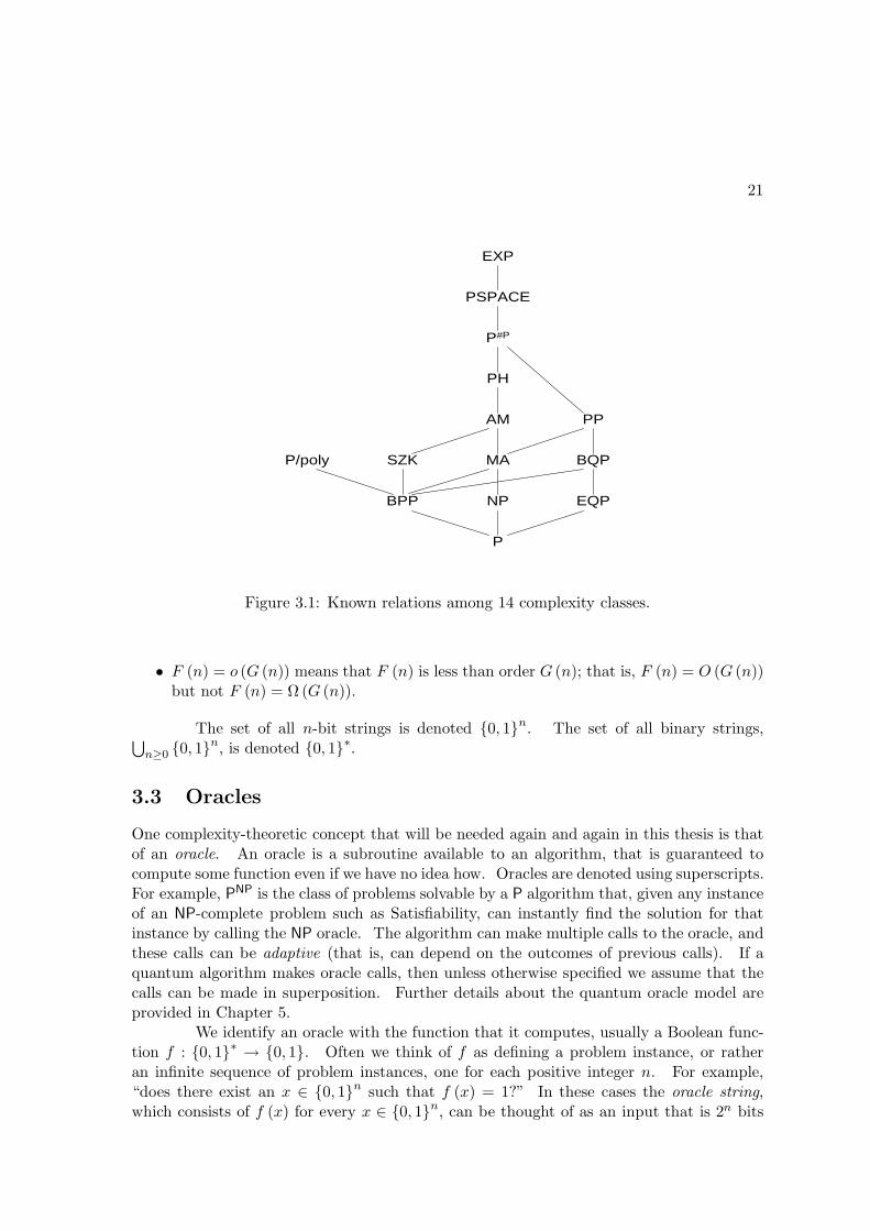
21

P

NP

MA

AM

PH

P#P

PSPACE

EXP

EQP

BQP

PP

BPP

SZKP/poly

Figure 3.1: Known relations among 14 complexity classes.

• F (n) = o (G (n)) means that F (n) is less than order G (n); that is, F (n) = O (G (n))but not F (n) = Ω (G (n)).

The set of all n-bit strings is denoted 0, 1n. The set of all binary strings,⋃n≥0 0, 1n, is denoted 0, 1∗.

3.3 Oracles

One complexity-theoretic concept that will be needed again and again in this thesis is thatof an oracle. An oracle is a subroutine available to an algorithm, that is guaranteed tocompute some function even if we have no idea how. Oracles are denoted using superscripts.For example, PNP is the class of problems solvable by a P algorithm that, given any instanceof an NP-complete problem such as Satisfiability, can instantly find the solution for thatinstance by calling the NP oracle. The algorithm can make multiple calls to the oracle, andthese calls can be adaptive (that is, can depend on the outcomes of previous calls). If aquantum algorithm makes oracle calls, then unless otherwise specified we assume that thecalls can be made in superposition. Further details about the quantum oracle model areprovided in Chapter 5.

We identify an oracle with the function that it computes, usually a Boolean func-tion f : 0, 1∗ → 0, 1. Often we think of f as defining a problem instance, or ratheran infinite sequence of problem instances, one for each positive integer n. For example,“does there exist an x ∈ 0, 1n such that f (x) = 1?” In these cases the oracle string,which consists of f (x) for every x ∈ 0, 1n, can be thought of as an input that is 2n bits

22

long instead of n bits. Of course, a classical algorithm running in polynomial time couldexamine only a tiny fraction of such an input, but maybe a quantum algorithm could dobetter. When discussing such questions, we need to be careful to distinguish between twofunctions: f itself, and the function of the oracle string that an algorithm is trying is tocompute.

23

Chapter 4

Quantum Computing Cheat Sheet

“Somebody says . . . ‘You know those quantum mechanical amplitudes you toldme about, they’re so complicated and absurd, what makes you think those areright? Maybe they aren’t right.’ Such remarks are obvious and are perfectlyclear to anybody who is working on this problem. It does not do any good topoint this out.”

—Richard Feynman, The Character of Physical Law [111]

Non-physicists often have the mistaken idea that quantum mechanics is hard.Unfortunately, many physicists have done nothing to correct that idea. But in newertextbooks, courses, and survey articles [18, 116, 177, 184, 235], the truth is starting to comeout: if you wish to understand the central ‘paradoxes’ of quantum mechanics, together withalmost the entire body of research on quantum information and computing, then you donot need to know anything about wave-particle duality, ultraviolet catastrophes, Planck’sconstant, atomic spectra, boson-fermion statistics, or even Schrodinger’s equation. All youneed to know is how to manipulate vectors whose entries are complex numbers. If that istoo difficult, then positive and negative real numbers turn out to suffice for most purposesas well. After you have mastered these vectors, you will then have some context if you wishto learn more about the underlying physics. But the historical order in which the ideaswere discovered is almost the reverse of the logical order in which they are easiest to learn!

What quantum mechanics says is that, if an object can be in either of two per-fectly distinguishable states, which we denote |0〉 and |1〉, then it can also be in a linear“superposition” of those states, denoted α |0〉 + β |1〉. Here α and β are complex numberscalled “amplitudes,” which satisfy |α|2 + |β|2 = 1. The asymmetric brackets | 〉 are called“Dirac ket notation”; one gets used to them with time.

If we measure the state α |0〉+β |1〉 in a standard way, then we see the “basis state”|0〉 with probability |α|2, and |1〉 with probability |β|2. Also, the state changes to whicheveroutcome we see—so if we see |0〉 and then measure again, nothing having happened in theinterim, we will still see |0〉. The two probabilities |α|2 and |β|2 sum to 1, as they oughtto. So far, we might as well have described the object using classical probabilities—forexample, “this cat is alive with probability 1/2 and dead with probability 1/2; we simplydon’t know which.”

24

The difference between classical probabilities and quantum amplitudes arises inhow the object’s state changes when we perform an operation on it. Classically, we canmultiply a vector of probabilities by a stochastic matrix, which is a matrix of nonnegativereal numbers each of whose columns sums to 1. Quantum-mechanically, we multiply thevector of amplitudes by a unitary matrix, which is a matrix of complex numbers that mapsany unit vector to another unit vector. (Equivalently, U is unitary if and only if its inverseU−1 equals its conjugate transpose U∗.) As an example, suppose we start with the state|0〉, which corresponds to the vector of amplitudes

[10

].

We then left-multiply this vector by the unitary matrix

U =

[1√2

− 1√2

1√2

1√2

],

which maps the vector to [1√2

1√2

],

and therefore the state |0〉 to

U |0〉 =1√2|0〉 +

1√2|1〉 .

If we now measured, we would see |0〉 with probability 1/2 and |1〉 with probability 1/2.The interesting part is what happens if we apply the same operation U a second time,without measuring. We get

[1√2

− 1√2

1√2

1√2

] [1√2

1√2

]=

[01

]

which is |1〉 with certainty (see Figure 4.1). Applying a “randomizing” operation to a“random” state produces a deterministic outcome! The reason is that, whereas probabilitiesare always nonnegative, amplitudes can be positive, negative, or even complex, and cantherefore cancel each other out. This interference of amplitudes can be considered thesource of all “quantum weirdness.”

4.1 Quantum Computers: N Qubits

The above description applied to “qubits,” or objects with only two distinguishable states.But it generalizes to objects with a larger number of distinguishable states. Indeed, inquantum computing we consider a system of N qubits, each of which can be |0〉 or |1〉. Wethen need to assign amplitudes to all 2N possible outcomes of measuring the qubits in orderfrom first to last. So the computer’s state has the form

|ψ〉 =∑

z∈0,1N

αz |z〉

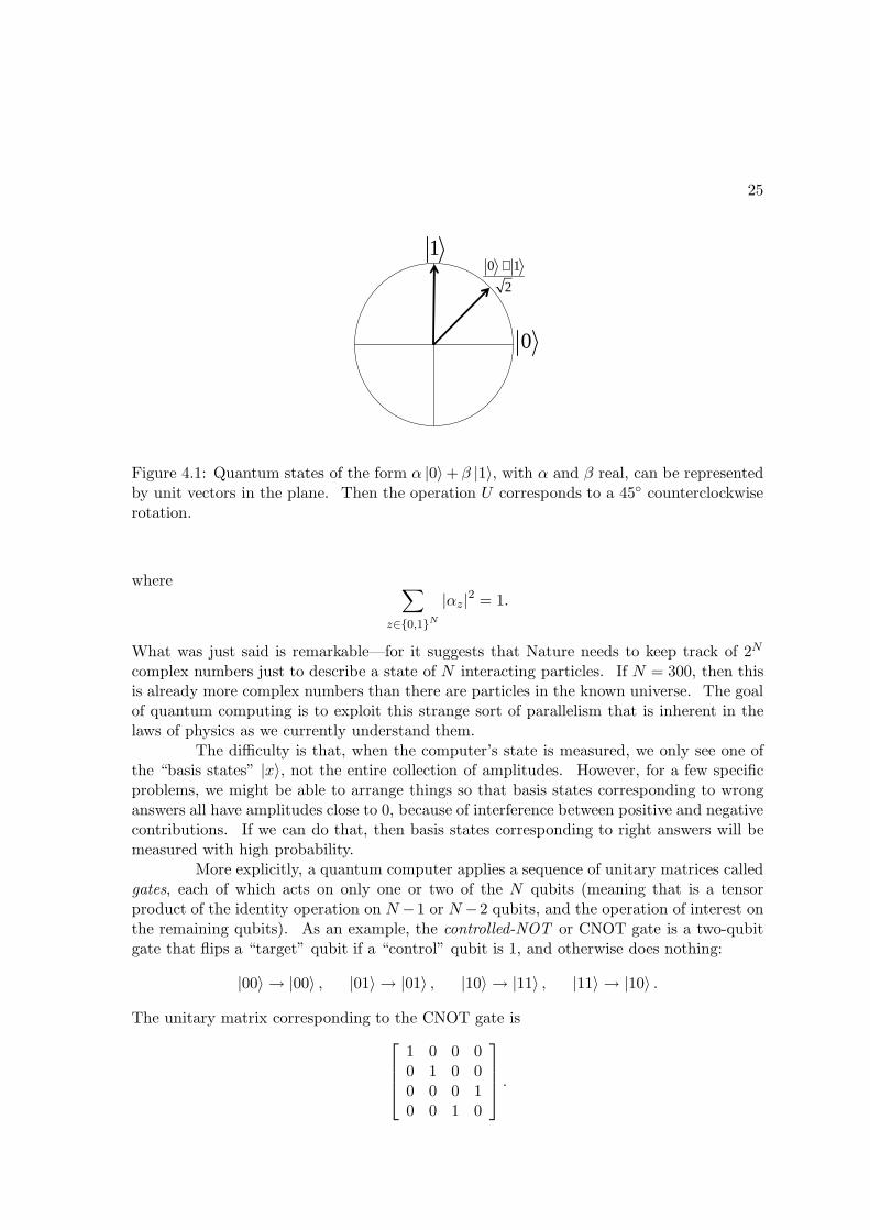
25

0

10 1

2

+

Figure 4.1: Quantum states of the form α |0〉+ β |1〉, with α and β real, can be representedby unit vectors in the plane. Then the operation U corresponds to a 45 counterclockwiserotation.

where ∑

z∈0,1N

|αz|2 = 1.

What was just said is remarkable—for it suggests that Nature needs to keep track of 2N

complex numbers just to describe a state of N interacting particles. If N = 300, then thisis already more complex numbers than there are particles in the known universe. The goalof quantum computing is to exploit this strange sort of parallelism that is inherent in thelaws of physics as we currently understand them.

The difficulty is that, when the computer’s state is measured, we only see one ofthe “basis states” |x〉, not the entire collection of amplitudes. However, for a few specificproblems, we might be able to arrange things so that basis states corresponding to wronganswers all have amplitudes close to 0, because of interference between positive and negativecontributions. If we can do that, then basis states corresponding to right answers will bemeasured with high probability.

More explicitly, a quantum computer applies a sequence of unitary matrices calledgates, each of which acts on only one or two of the N qubits (meaning that is a tensorproduct of the identity operation on N −1 or N −2 qubits, and the operation of interest onthe remaining qubits). As an example, the controlled-NOT or CNOT gate is a two-qubitgate that flips a “target” qubit if a “control” qubit is 1, and otherwise does nothing:

|00〉 → |00〉 , |01〉 → |01〉 , |10〉 → |11〉 , |11〉 → |10〉 .

The unitary matrix corresponding to the CNOT gate is

1 0 0 00 1 0 00 0 0 10 0 1 0

.

26

Adleman, DeMarrais, and Huang [16] showed that the CNOT gate, together with the one-qubit gate [

35 −4

545

35

],

constitute a universal set of quantum gates, in that they can be used to approximate anyother gate to any desired accuracy. Indeed, almost any set of one- and two-qubit gates isuniversal in this sense [96].

A quantum circuit is just a sequence of gates drawn from a finite universal set.Without loss of generality, we can take the circuit’s output to be the result of a singlemeasurement after all gates have been applied; that is, z ∈ 0, 1N with probability |αz|2.(If a binary output is needed, we simply throw away the last N − 1 bits of z.) It is knownthat allowing intermediate measurements does not yield any extra computational power[55]. The circuit is polynomial-size if both N and the number of gates are upper-boundedby a polynomial in the length n of the input.

We can now define the important complexity class BQP, or Bounded-Error Quan-tum Polynomial-Time. Given an input x ∈ 0, 1n, first a polynomial-time classical algo-rithm A prepares a polynomial-size quantum circuit Ux. (The requirement that the circuititself be efficiently preparable is called uniformity.) Then Ux is applied to the “all-0” initialstate |0〉⊗N . We say a language L ⊆ 0, 1n is in BQP if there exists an A such that for allx,

(i) If x ∈ L then Ux outputs ‘1’ with probability at least 2/3.

(ii) If x /∈ L then Ux outputs ‘0’ with probability at least 2/3.

By running Ux multiple times and taking the majority answer, we can boost theprobability of success from 2/3 to 1 − 2−p(n) for any polynomial p.

BQP was first defined in a 1993 paper by Bernstein and Vazirani [55].1 That papermarked a turning point. Before, quantum computing had been an idea, explored in pio-neering work by Deutsch [92], Feynman [110], and others. Afterward, quantum computingwas a full-fledged model in the sense of computational complexity theory, which could bemeaningfully compared against other models. For example, Bernstein and Vazirani showedthat BPP ⊆ BQP ⊆ P#P: informally, quantum computers are at least as powerful as classi-cal probabilistic computers, and at most exponentially more powerful. (The containmentBQP ⊆ P#P was later improved to BQP ⊆ PP by Adleman, DeMarrais, and Huang [16].)

Bernstein and Vazirani also gave an oracle problem called Recursive Fourier Sam-pling (RFS), and showed that it requires nΩ(logn) classical probabilistic queries but only nquantum queries. This provided the first evidence that quantum computers are strictlymore powerful than classical probabilistic computers, i.e. that BPP 6= BQP. Soon after-ward, Simon [222] widened the gap to polynomial versus exponential, by giving an ora-cle problem that requires Ω

(2n/2

)classical probabilistic queries but only O (n) quantum

1As a historical note, Bernstein and Vazirani [55] defined BQP in terms of “quantum Turing machines.”However, Yao [248] showed that Bernstein and Vazirani’s definition is equivalent to the much simpler onegiven here. Also, Berthiaume and Brassard [57] had implicitly defined EQP (Exact Quantum Polynomial-Time) a year earlier, and had shown that it lies outside P and even NP relative to an oracle.

27

queries. However, these results attracted limited attention because the problems seemedartificial.

People finally paid attention when Shor [221] showed that quantum computerscould factor integers and compute discrete logarithms in polynomial time. The securityof almost all modern cryptography rests on the presumed intractability of those two prob-lems. It had long been known [179] that factoring is classically reducible to the followingproblem: given oracle access to a periodic function f : 1, . . . , R → 1, . . . , R, where R isexponentially large, find the period of f . Shor gave an efficient quantum algorithm for thisoracle problem, by exploiting the quantum Fourier transform, a tool that had earlier beenused by Simon. (The algorithm for the discrete logarithm problem is more complicatedbut conceptually similar.)

Other results in the “quantum canon,” such as Grover’s algorithm [141] and meth-ods for quantum error-correction and fault-tolerance [20, 80, 134, 161, 227], will be discussedin this thesis as the need arises.

4.2 Further Concepts

This section summarizes “fancier” quantum mechanics concepts, which are needed for PartII and for Chapter 10 of Part I (which deals with quantum advice). They are not neededfor the other chapters in Part I.

Tensor Product. If |ψ〉 and |ϕ〉 are two quantum states, then their tensorproduct, denoted |ψ〉⊗ |ϕ〉 or |ψ〉 |ϕ〉, is just a state that consists of |ψ〉 and |ϕ〉 next to eachother. For example, if |ψ〉 = α |0〉 + β |1〉 and |ϕ〉 = γ |0〉 + δ |1〉, then

|ψ〉 |ϕ〉 = (α |0〉 + β |1〉) (γ |0〉 + δ |1〉) = αγ |00〉 + αδ |01〉 + βγ |10〉 + βδ |11〉 .

Inner Product. The inner product between two states |ψ〉 = α1 |1〉+· · ·+αN |N〉and |ϕ〉 = β1 |1〉 + · · · + βN |N〉 is defined as

〈ψ|ϕ〉 = α∗1β1 + · · · + α∗

NβN

where ∗ denotes complex conjugate. The inner product satisfies all the expected properties,such as 〈ψ|ψ〉 = 1 and

〈ψ| (|ϕ〉 + |φ〉) = 〈ψ|ϕ〉 + 〈ψ|φ〉 .If 〈ψ|ϕ〉 = 0 then we say |ψ〉 and |ϕ〉 are orthogonal.

General Measurements. In principle, we can choose any orthogonal basis ofstates |ϕ1〉 , . . . , |ϕN 〉 in which to measure a state |ψ〉. (Whether that measurementcan actually be performed efficiently is another matter.) Then the probability of obtainingoutcome |ϕj〉 is |〈ψ|ϕj〉|2. We can even measure in a non-orthogonal basis, a concept calledPositive Operator Valued Measurements (POVM’s) that I will not explain here. None ofthese more general measurements increase the power of the quantum computing model,since we can always produce the same effect by first applying a unitary matrix (possiblyusing additional qubits called ancillas), and then measuring in a “standard” basis such as|1〉 , . . . , |N〉.

28

Mixed States. Superposition states, such as α |0〉 + β |1〉, are also called purestates. This is to distinguish them from mixed states, which are the most general kindof state in quantum mechanics. Mixed states are just classical probability distributionsover pure states. There is a catch, though: any mixed state can be decomposed intoa probability distribution over pure states in infinitely many nonequivalent ways. Forexample, if we have a state that is |0〉 with probability 1/2 and |1〉 with probability 1/2, thenno experiment could ever distinguish it from a state that is (|0〉 + |1〉) /

√2 with probability

1/2 and (|0〉 − |1〉) /√

2 with probability 1/2. For regardless of what orthogonal basis wemeasured in, the two possible outcomes of measuring would both occur with probability1/2. Therefore, this state is called the one-qubit maximally mixed state.

Density Matrices. We can represent mixed states using a formalism calleddensity matrices. The outer product of |ψ〉 = α1 |1〉 + · · · + αN |N〉 with itself, denoted|ψ〉〈ψ|, is an N × N complex matrix whose (i, j) entry is αiα

∗j . Now suppose we have a

state that is |ϕ〉 = α |0〉 + β |1〉 with probability p, and |φ〉 = γ |0〉 + δ |1〉 with probability1 − p. We represent the state by a Hermitian positive definite matrix ρ with trace 1, asfollows:

ρ = p |ϕ〉〈ϕ| + (1 − p) |φ〉〈φ| = p

[αα∗ αβ∗

βα∗ ββ∗

]+ (1 − p)

[γγ∗ γδ∗

δγ∗ δδ∗

].

When we apply a unitary operation U , the density matrix ρ changes to UρU−1. Whenwe measure in the standard basis, the probability of outcome |j〉 is the jth diagonal entryof ρ. Proving that these rules are the correct ones, and that a density matrix really is aunique description of a mixed state, are “exercises for the reader” (which as always meansthe author was too lazy). Density matrices will mainly be used in Chapter 10.

Trace Distance. Suppose you are given a system that was prepared in state ρwith probability 1/2, and σ with probability 1/2. After making a measurement, you mustguess which state the system was prepared in. What is the maximum probability that youwill be correct? The answer turns out to be

1 + ‖ρ− σ‖tr

2

where ‖ρ− σ‖tr is the trace distance between ρ and σ, defined as 12

∑i |λi| where λ1, . . . , λN

are the eigenvalues of ρ− σ.Entanglement. Suppose ρ is a joint state of two systems. If ρ can be written as

a probability distribution over pure states of the form |ψ〉 ⊗ |ϕ〉, then we say ρ is separable;otherwise ρ is entangled.

Hamiltonians. Instead of discrete unitary operations, we can imagine that aquantum state evolves in time by a continuous rotation called a Hamiltonian. A Hamil-tonian is an N × N Hermitian matrix H. To find the unitary operation U (t) that iseffected by “leaving H on” for t time steps, the rule2 is U (t) = e−iHt. The only place Iuse Hamiltonians is in Chapter 14, and even there the use is incidental.

2Here Planck’s constant is set equal to 1 as always.

29

Part I

Limitations of QuantumComputers

30

Chapter 5

Introduction

“A quantum possibility is less real than a classical reality, but more real thana classical possibility.”

—Boris Tsirelson [231]

Notwithstanding accounts in the popular press, a decade of research has made itclear that quantum computers would not be a panacea. In particular, we still do not have aquantum algorithm to solve NP-complete problems in polynomial time. But can we provethat no such algorithm exists, i.e. that NP 6⊂ BQP? The difficulty is that we can’t evenprove no classical algorithm exists; this is the P versus NP question. Of course, we couldask whether NP 6⊂ BQP assuming that P 6= NP—but unfortunately, even this conditionalquestion seems far beyond our ability to answer. So we need to refine the question evenfurther: can quantum computers solve NP-complete problems in polynomial time, by bruteforce?

What is meant by “brute force” is the following. In Shor’s factoring algorithm[221], we prepare a superposition of the form

1√R

R∑

r=1

|r〉 |g (r)〉

where g (r) = xr modN for some x,N . But as far as the key step of the algorithm isconcerned, the function g is a “black box.” Given any superposition like the one above,the algorithm will find the period of g assuming g is periodic; it does not need furtherinformation about how g was computed. So in the language of Section 3.3, we might aswell say that g is computed by an oracle.

Now suppose we are given a Boolean formula ϕ over n variables, and are asked todecide whether ϕ is satisfiable. One approach would be to exploit the internal structureof ϕ: “let’s see, if I set variable x37 to TRUE, then this clause here is satisfied, but thoseother clauses aren’t satisfied any longer . . . darn!” However, inspired by Shor’s factoringalgorithm, we might hope for a cruder quantum algorithm that treats ϕ merely as an oracle,mapping an input string x ∈ 0, 1n to an output bit ϕ (x) that is 1 if and only if x satisfiesϕ. The algorithm would have to decide whether there exists an x ∈ 0, 1n such that

31

ϕ (x) = 1, using as few calls to the ϕ oracle as possible, and not learning about ϕ in anyother way. This is what is meant by brute force.

A fundamental result of Bennett, Bernstein, Brassard, and Vazirani [51] says thatno brute-force quantum algorithm exists to solve NP-complete problems in polynomial time.In particular, for some probability distribution over oracles, any quantum algorithm needsΩ(2n/2

)oracle calls to decide, with at least a 2/3 chance of being correct, whether there

exists an x ∈ 0, 1n such that ϕ (x) = 1. On a classical computer, of course, Θ (2n) oraclecalls are necessary and sufficient. But as it turns out, Bennett et al.’s quantum lower boundis tight, since Grover’s quantum search algorithm [141] can find a satisfying assignment (ifit exists) quadratically faster than any classical algorithm. Amusingly, Grover’s algorithmwas proven optimal before it was discovered to exist!

A recurring theme in this thesis is the pervasiveness of Bennett et al.’s finding. Iwill show that, even if a problem has considerably more structure than the basic Groversearch problem, even if “quantum advice states” are available, or even if we could examinethe entire history of a hidden variable, still any brute-force quantum algorithm would takeexponential time.

5.1 The Quantum Black-Box Model

The quantum black-box model formalizes the idea of a brute-force algorithm. For the timebeing, suppose that a quantum algorithm’s goal is to evaluate f (X), where f : 0, 1n →0, 1 is a Boolean function and X = x1 . . . xn is an n-bit string. Then the algorithm’sstate at any time t has the form ∑

i,z

α(t)i,z |i, z〉 .

Here i ∈ 1, . . . , N is the index of an oracle bit xi to query, and z is an arbitrarily largestring of bits called the “workspace,” containing whatever information the algorithm wantsto store there. The state evolves in time via an alternating sequence of algorithm steps andquery steps. An algorithm step multiplies the vector of αi,z’s by an arbitrary unitary matrixthat does not depend on X. It does not matter how many quantum gates would be neededto implement this matrix. A query step maps each basis state |i, z〉 to |i, z ⊕ xi〉, effecting

the transformation α(t+1)i,z = α

(t)i,z⊕xi

. Here z ⊕ xi is the string z, with xi exclusive-OR’edinto a particular location in z called the “answer bit.” The reason exclusive-OR is used isthat the query step has to be reversible, or else it would not be unitary.

At the final step T , the state is measured in the standard basis, and the output ofthe algorithm is taken to be (say) z1, the first bit of z. The algorithm succeeds if

∑

i,z : z1=f(X)

∣∣∣α(T )i,z

∣∣∣2≥ 2

3

for all X ∈ 0, 1n. Here the constant 2/3 is arbitrary. Then the (bounded-error) quantumquery complexity of f , denoted Q2 (f), is the minimum over all quantum algorithms A thatsucceed at evaluating f , of the number of queries to f made by A. Here the ‘2’ representsthe fact that the error probability is two-sided. One can compare Q2 (f) with Q0 (f),

32

or zero-error quantum query complexity; R2 (f), or bounded-error classical randomizedquery complexity; and D (f), or deterministic query complexity, among other complexitymeasures. Chapter 8 will define many such measures and compare them in detail.

As a simple example of the black-box model, let OR (x1, . . . , xn) = x1 ∨ · · · ∨ xn.Then Grover’s algorithm [141] implies that Q2 (OR) = O (

√n), while the lower bound of

Bennett et al. [51] implies that Q2 (OR) = Ω (√n). By comparison, D (OR) = R2 (OR) =

Θ (n).The quantum black-box model has some simple generalizations, which I will use

when appropriate. First, f can be a partial function, defined only on a subset of 0, 1n(so we obtain what is called a promise problem). Second, the xi’s do not need to be bits;in Chapters 6 and 7 they will take values from a larger range. Third, in Chapter 7 theoutput will not be Boolean, and there will generally be more than one valid output (so weobtain what is called a relation problem).

5.2 Oracle Separations

“I do believe itAgainst an oracle.”—Shakespeare, The Tempest

Several times in this thesis, I will use a lower bound on quantum query complexityto show that a complexity class is not in BQP “relative to an oracle.” The method for turningquery complexity lower bounds into oracle separations was invented by Baker, Gill, andSolovay [41] to show that there exists an oracle A relative to which PA 6= NPA. Basically,they encoded into A an infinite sequence of exponentially hard search problems, one foreach input length n, such that (i) a nondeterministic machine can solve the nth problemin time polynomial in n, but (ii) any deterministic machine would need time exponentialin n. They guaranteed (ii) by “diagonalizing” against all possible deterministic machines,similarly to how Turing created an uncomputable real number by diagonalizing against allpossible computable reals. Later, Bennett and Gill [54] showed that a simpler way toguarantee (ii) is just to choose the search problems uniformly at random. Throughout thethesis, I will cavalierly ignore such issues, proceeding immediately from a query complexitylower bound to the statement of the corresponding oracle separation.

The point of an oracle separation is to rule out certain approaches to solvingan open problem in complexity theory. For example, the Baker-Gill-Solovay theoremimplies that the standard techniques of computability theory, which relativize (that is, are“oblivious” to the presence of an oracle), cannot be powerful enough to show that P = NP.Similarly, the result of Bennett et al. [51] that Q2 (OR) = Ω (

√n) implies that there exists

an oracle A relative to which NPA 6⊂ BQPA. While this does not show that NP 6⊂ BQP,it does show that any proof of NP ⊆ BQP would have to use “non-relativizing” techniquesthat are unlike anything we understand today.

However, many computer scientists are skeptical that anything can be learnedfrom oracles. The reason for their skepticism is that over the past 15 years, they haveseen several examples of non-relativizing results in classical complexity theory. The most

33

famous of these is Shamir’s Theorem [217, 173] that PSPACE ⊆ IP, where IP is the class ofproblems that have interactive proof systems, meaning that if the answer for some instanceis “yes,” then a polynomial-time verifier can become convinced of that fact to any desiredlevel of confidence by exchanging a sequence of messages with an omniscient prover.1 Bycontrast, oracles had been known relative to which not even coNP, let alone PSPACE, iscontained in IP [119]. So why should we ever listen to oracles again, if they got interactiveproofs so dramatically wrong?

My answer is threefold. First, essentially all quantum algorithms that we knowtoday—from Shor’s algorithm, as discussed previously, to Grover’s algorithm, to the quan-tum adiabatic algorithm2 [108], to the algorithms of Hallgren [143] and van Dam, Hallgren,and Ip [90]—are oracle algorithms at their core. We do not know of any non-relativizingquantum algorithm technique analogous to the arithmetization technique that was used toprove PSPACE ⊆ IP. If such a technique is ever discovered, I will be one of the first towant to learn it.

The second response is that without oracle results, we do not have even the be-ginnings of understanding. Once we know (for example) that SZK 6⊂ BQP relative to anoracle, we can then ask the far more difficult unrelativized question, knowing somethingabout the hurdles that any proof of SZK ⊆ BQP would have to overcome.

The third response is that “the proof of the pudding is in the proving.” In otherwords, the real justification for the quantum black-box model is not the a priori plausibilityof its assumptions, but the depth and nontriviality of what can be (and has been) provedin it. For example, the result that coNP 6⊂ IP relative to an oracle [119] does not tell usmuch about interactive proof systems. For given an exponentially long oracle string X, itis intuitively obvious that nothing a prover could say could convince a classical polynomial-time verifier that X is the all-0 string, even if the prover and verifier could interact. Theonly issue is how to formalize that obvious fact by diagonalizing against all possible proofsystems. By contrast, the quantum oracle separations that we have are not intuitivelyobvious in the same way; or rather, the act of understanding them confers an intuitionwhere none was previously present.

1Arora, Impagliazzo, and Vazirani [36] claim the Cook-Levin Theorem, that Satisfiability is NP-complete,as another non-relativizing result. But this hinges on what we mean by “non-relativizing,” far more thanthe PSPACE ⊆ IP example.

2Given an assignment x to a 3SAT formula ϕ, the adiabatic algorithm actually queries an oracle thatreturns the number of clauses of ϕ that x satisfies, not just whether x satisfies ϕ or not. Furthermore, vanDam, Mosca, and Vazirani [91] have shown such an oracle is sufficient to reconstruct ϕ. On the other hand,the adiabatic algorithm itself would be just as happy with a fitness landscape that did not correspond toany 3SAT instance, and that is what I mean by saying that it is an oracle algorithm at the core.

34

Chapter 6

The Collision Problem

The collision problem of size n, or Coln, is defined as follows. Let X = x1 . . . xnbe a sequence of n integers drawn from 1, . . . , n, with n even. We are guaranteed thateither

(1) X is one-to-one (that is, a permutation of 1, . . . , n), or

(2) X is two-to-one (that is, each element of 1, . . . , n appears in X twice or not at all).

The problem is to decide whether (1) or (2) holds. (A variant asks us to find acollision in a given two-to-one function. Clearly a lower bound for the collision problem asdefined above implies an equivalent lower bound for this variant.) Because of its simplicity,the collision problem was widely considered a benchmark for our understanding of quantumquery complexity.

I will show that Q2 (Coln) = Ω(n1/5

), where Q2 (f) is the bounded-error quantum

query complexity of function f . The best known upper bound, due to Brassard, Høyer,and Tapp [68], is O

(n1/3

)(see Section 2.1.1). Previously, though, no lower bound better

than the trivial Ω (1) bound was known. How great a speedup quantum computers yieldfor the problem was apparently first asked by Rains [195].

Previous lower bound techniques failed for the problem because they depended ona function’s being sensitive to many disjoint changes to the input. For example, Beals et al.

[45] showed that for all total Boolean functions f , Q2 (f) = Ω(√

bs (f)), where bs (f) is the

block sensitivity, defined by Nisan [185] to be, informally, the maximum number of disjointchanges (to any particular input X) to which f is sensitive. In the case of the collisionproblem, though, every one-to-one input differs from every two-to-one input in at least n/2places, so the block sensitivity is O (1). Ambainis’s adversary method [27] faces a relatedobstacle. In that method we consider the algorithm and input as a bipartite quantumstate, and upper-bound how much the entanglement of the state can increase via a singlequery. But under the simplest measures of entanglement, it turns out that the algorithmand input can become almost maximally entangled after O (1) queries, again because everyone-to-one input is far from every two-to-one input.1

1More formally, the adversary method cannot prove any lower bound on Q2 (f) better than RC (f),where RC(f) is the randomized certificate complexity of f (to be defined in Chapter 8). But for the

35

My proof is an adaptation of the polynomial method, introduced to quantum com-puting by Beals et al. [45]. Their idea was to reduce questions about quantum algorithmsto easier questions about multivariate polynomials. In particular, if a quantum algorithmmakes T queries, then its acceptance probability is a polynomial over the input bits ofdegree at most 2T . So by showing that any polynomial approximating the desired outputhas high degree, one obtains a lower bound on T .

To lower-bound the degree of a multivariate polynomial, a key technical trick is toconstruct a related univariate polynomial. Beals et al. [45], using a lemma due to Minskyand Papert [180], replace a polynomial p (X) (where X is a bit string) by q (|X|) (where|X| denotes the Hamming weight of X), satisfying

q (k) = EX|X|=k

p (X)

and deg (q) ≤ deg (p).Here I construct the univariate polynomial in a different way. I consider a uniform

distribution over g-to-one inputs, where g might be greater than 2. Even though theproblem is to distinguish g = 1 from g = 2, the acceptance probability must lie in theinterval [0, 1] for all g, and that is a surprisingly strong constraint. I show that theacceptance probability is close to a univariate polynomial in g of degree at most 2T . I thenobtain a lower bound by generalizing a classical approximation theory result of Ehlich andZeller [106] and Rivlin and Cheney [206]. Much of the proof deals with the complicationthat g does not divide n in general.

Shortly after this work was completed, Shi [220] improved it to give a tight lowerbound of Ω

(n1/3

)for the collision problem, when the xi range from 1 to 3n/2 rather than

from 1 to n. For a range of size n, his bound was Ω(n1/4

). Subsequently Kutin [163]

and Ambainis [29] showed a lower bound of Ω(n1/3

)for a range of size n as well. By a

simple reduction, these results imply a lower bound of Ω(n2/3

)for the element distinctness

problem—that of deciding whether there exist i 6= j such that xi = xj. The previous bestknown lower bound was Ω

(n1/2

), and at the time of Shi’s work, the best known upper

bound was O(n3/4

), due to Buhrman et al. [77]. Recently, however, Ambainis [30] gave a

novel algorithm based on quantum walks that matches the n2/3 lower bound.The chapter is organized as follows. Section 6.1 motivates the collision lower bound

within quantum computing, pointing out connections to collision-resistant hash functions,the nonabelian hidden subgroup problem, statistical zero-knowledge, and information era-sure. Section 6.2 gives technical preliminaries, Section 6.3 proves the crucial fact that theacceptance probability is “almost” a univariate polynomial, and Section 6.4 completes thelower bound argument. I conclude in Section 6.6 with some open problems. In Section 6.5I show a lower bound of Ω

(n1/7

)for the set comparison problem, a variant of the collision

problem needed for the application to information erasure.

collision function, RC (Coln) = O (1).

36

6.1 Motivation

In Chapter 1 I listed seven implications of the collision lower bound; this section discusses afew of those implications in more detail. The implication that motivated me personally—concerning the computational power of so-called hidden-variable theories—is deferred toChapter 16.

6.1.1 Oracle Hardness Results

The original motivation for the collision problem was to model (strongly) collision-resistanthash functions in cryptography. There is a large literature on collision-resistant hashing;see [203, 42] for example. When building secure digital signature schemes, it is useful tohave a family of hash functions Hi, such that finding a distinct (x, y) pair with Hi (x) =Hi (y) is computationally intractable. A quantum algorithm for finding collisions usingO (polylog (n)) queries would render all hash functions insecure against quantum attackin this sense. (Shor’s algorithm [221] already renders hash functions based on modulararithmetic insecure.) My result indicates that collision-resistant hashing might still bepossible in a quantum setting.

The collision problem also models the nonabelian hidden subgroup problem, ofwhich graph isomorphism is a special case. Given a group G and subgroup H ≤ G,suppose we have oracle access to a function f : G → N such that for all g1, g2 ∈ G,f (g1) = f (g2) if and only if g1 and g2 belong to the same coset of H. Is there then anefficient quantum algorithm to determine H? If G is abelian, the work of Simon [222], Shor[221], and Kitaev [154] implies an affirmative answer. If G is nonabelian, though, efficientquantum algorithms are known only for special cases [107, 140]. An O (polylog (n))-queryalgorithm for the collision problem would yield a polynomial-time algorithm to distinguish|H| = 1 from |H| = 2, which does not exploit the group structure at all. My result impliesthat no such algorithm exists.

Finally, the collision lower bound implies that there exists an oracle relative towhich SZK 6⊂ BQP, where SZK is the class of problems having statistical zero-knowledgeproof protocols. For suppose that a verifier V and prover P both have oracle access toa sequence X = x1 . . . x2n , which is either one-to-one or two-to-one. To verify with zeroknowledge that X is one-to-one, V can repeatedly choose an i ∈R 1, . . . , 2n and send xi toP , whereupon P must send i back to V . Thus, using standard diagonalization techniques,one can produce an oracle A such that SZKA 6⊂ BQPA.

6.1.2 Information Erasure

Let f : 0, 1n → 0, 1m with m ≥ n be a one-to-one function. Then we can consider twokinds of quantum oracle for f :

(A) a standard oracle, one that maps |x〉 |z〉 to

|x〉 |z ⊕ f (x)〉, or

(B) an erasing oracle (as proposed by Kashefi et al. [152]), which maps |x〉 to |f (x)〉, ineffect “erasing” |x〉.

37

Intuitively erasing oracles seem at least as strong as standard ones, though it isnot clear how to simulate the latter with the former without also having access to an oraclethat maps |y〉 to

∣∣f−1 (y)⟩. The question that concerns us here is whether erasing oracles

are more useful than standard ones for some problems. One-way functions provide a clue:if f is one-way, then (by assumption) |x〉 |f (x)〉 can be computed efficiently, but if |f (x)〉could be computed efficiently given |x〉 then so could |x〉 given |f (x)〉, and hence f could beinverted. But can we find, for some problem, an exponential gap between query complexitygiven a standard oracle and query complexity given an erasing oracle?

In Section 6.5 I extend the collision lower bound to show an affirmative answer.Define the set comparison problem of size n, or SetCompn, as follows. We are given as inputtwo sequences, X = x1 . . . xn and Y = y1 . . . yn, such that for each i, xi, yi ∈ 1, . . . , 2n.A query has the form (b, i), where b ∈ 0, 1 and i ∈ 1, . . . , n, and produces as output(0, xi) if b = 0 and (1, yi) if b = 1. Sequences X and Y are both one-to-one; that is, xi 6= xjand yi 6= yj for all i 6= j. We are furthermore guaranteed that either

(1) X and Y are equal as sets (that is, x1, . . . , xn = y1, . . . , yn) or

(2) X and Y are far as sets (that is,

|x1, . . . , xn ∪ y1, . . . , yn| ≥ 1.1n).

As before the problem is to decide whether (1) or (2) holds.This problem can be solved with high probability in a constant number of queries

using an erasing oracle, by using a trick similar to that of Watrous [239] for verifying groupnon-membership. First, using the oracle, we prepare the uniform superposition

1√2n

∑

i∈1,...,n(|0〉 |xi〉 + |1〉 |yi〉) .

We then apply a Hadamard gate to the first register, and finally we measure the first register.If X and Y are equal as sets, then interference occurs between every (|0〉 |z〉 , |1〉 |z〉) pairand we observe |0〉 with certainty. But if X and Y are far as sets, then basis states |b〉 |z〉with no matching |1 − b〉 |z〉 have probability weight at least 1/10, and hence we observe |1〉with probability at least 1/20.

In Section 6.5 I sketch a proof that Q2 (SetCompn) = Ω(n1/7

); that is, no efficient

quantum algorithm using a standard oracle exists for this problem. Recently, Midrijanis

[178] gave a lower bound of Ω((n/ log n)1/5

)not merely for the set comparison problem,

but for the set equality problem (where we are promised that X and Y are either equal ordisjoint).

6.2 Preliminaries

Let A be a quantum query algorithm as defined in Section 5.1. A basis state of A is written|i, z〉. Then a query replaces each |i, z〉 by |i, z ⊕ xi〉, where xi is exclusive-OR’ed into somespecified location of z. Between queries, the algorithm can perform any unitary operation

38

that does not depend on the input. Let T be the total number of queries. Also, assumefor simplicity that all amplitudes are real; this restriction is without loss of generality [55].

Let α(t)i,z (X) be the amplitude of basis state |i, z〉 after t queries when the input

is X. Also, let ∆ (xi, h) = 1 if xi = h, and ∆ (xi, h) = 0 if xi 6= h. Let P (X) be theprobability that A returns “two-to-one” when the input is X. Then we obtain a simplevariant of a lemma due to Beals et al. [45].

Lemma 1 P (X) is a multilinear polynomial of degree at most 2T over the ∆ (xi, h).

Proof. We show, by induction on t, that for all basis states |i, z〉, the amplitude

α(t)i,z (X) is a multilinear polynomial of degree at most t over the ∆ (xi, h). Since P (X) is

a sum of squares of α(t)i,z ’s, the lemma follows.

The base case (t = 0) holds since, before making any queries, each α(t)i,z is a degree-

0 polynomial over the ∆ (xi, h). A unitary transformation on the algorithm part replaces

each α(t)i,z by a linear combination of α

(t)i,z ’s, and hence cannot increase the degree. Suppose

the lemma holds prior to the tth query. Then

α(t+1)i,z (X) =

∑

1≤h≤nα

(t)i,z⊕h (X) ∆ (xi, h) ,

and we are done.

6.3 Reduction to Bivariate Polynomial

Call the point (g,N) ∈ <2 an (n, T )-quasilattice point if and only if

(1) g and N are integers, with g dividing N ,

(2) 1 ≤ g ≤ √n,

(3) n ≤ N ≤ n+ n/ (10T ), and

(4) if g = 1 then N = n.

For quasilattice point (g,N), define Dn (g,N) to be the uniform distribution overall size-n subfunctions of g-to-1 functions having domain 1, . . . , N and range a subsetof 1, . . . , n. More precisely: to draw an X from Dn (g,N), we first choose a set S ⊆1, . . . , n with |S| = N/g ≤ n uniformly at random. We then choose a g-to-1 functionX = x1 . . . xN from 1, . . . , N to S uniformly at random. Finally we let xi = xi for each1 ≤ i ≤ n.

Let P (g,N) be the probability that algorithm A returns z = 2 when the input ischosen from Dn (g,N):

P (g,N) = EXX∈Dn(g,N)

[P (X)] .

We then have the following surprising characterization:

39

Lemma 2 For all sufficiently large n and if T ≤ √n/3, there exists a bivariate polynomial

q (g,N) of degree at most 2T such that if (g,N) is a quasilattice point, then

|P (g,N) − q (g,N)| < 0.182

(where the constant 0.182 can be made arbitrarily small by adjusting parameters).

Proof. Let I be a product of ∆ (xi, h) variables, with degree r (I), and let I (X) ∈0, 1 be I evaluated on input X. Then define

γ (I, g,N) = EXX∈Dn(g,N)

[I (X)]

to be the probability that monomial I evaluates to 1 when the input is drawn from Dn (g,N).Then by Lemma 1, P (X) is a polynomial of degree at most 2T over X, so

P (g,N) = EXX∈Dn(g,N)

[P (X)]

= EXX∈Dn(g,N)

∑

I:r(I)≤2t

βII (X)

=∑

I:r(I)≤2T

βIγ (I, g,N)

for some coefficients βI .We now calculate γ (I, g,N). Assume without loss of generality that for all

∆ (xi, h1) ,∆ (xj, h2) ∈ I, either i 6= j or h1 = h2, since otherwise γ (I, g,N) = 0.Define the “range” Z (I) of I to be the set of all h such that ∆ (xi, h) ∈ I. Let

w (I) = |Z (I)|; then we write Z (I) =z1, . . . , zw(I)

. Clearly γ (I, g,N) = 0 unless

Z (I) ∈ S, where S is the range of X. By assumption,

N

g≥ n√

n≥ 2T ≥ r (I)

so the number of possible S is

(n

N/g

)and, of these, the number that contain Z is

(n− w (I)

N/g −w (I)

).

Then, conditioned on Z ∈ S, what is the probability that γ (I, g,N) = 1? The

total number of g-to-1 functions with domain size N is N !/ (g!)N/g , since we can permutethe N function values arbitrarily, but must not count permutations that act only withinthe N/g constant-value blocks of size g.

Among these functions, how many satisfy γ (I, g,N) = 1? Suppose that, for each1 ≤ j ≤ w (I), there are rj (I) distinct i such that ∆ (xi, zj) ∈ I. Clearly

r1 (I) + · · · + rw(I) (I) = r (I) .

40

Then we can permute the (N − r (I))! function values outside of I arbitrarily, but must notcount permutations that act only within the N/g constant-value blocks, which have sizeeither g or g − ri (I) for some i. So the number of functions for which γ (I, g,N) = 1 is

(N − r (I))!

(g!)N/g−w(I)∏w(I)

i=1(g − ri (I))!

.

Putting it all together,

γ (I, g,N) =

(n− w (I)

N/g − w (I)

)

(n

N/g

) · (N − r (I))! (g!)N/g

(g!)N/g−w(I)N !∏w(I)

i=1(g − ri (I))!

=(N − r (I))! (n− w (I))! (N/g)!

N !n! (N/g − w (I))!· (g!)w(I)

∏w(I)

i=1(g − ri (I))!

=(N − r (I))!

N !

(n− w (I))!

n!·w(I)−1∏

i=0

(N

g− i

)w(I)∏

i=1

g

ri(I)−1∏

j=1

(g − j)

=(N − 2T )!n!

N ! (n− 2T )!qn,T,I (g,N)

where

qn,T,I (g,N) =(n− w (I))! (n− 2T )!

(n!)2·

2T−1∏

i=r(I)

(N − i)

w(I)−1∏

i=0

(N − gi)

w(I)∏

i=1

ri(I)−1∏

j=1

(g − j)

is a bivariate polynomial of total degree at most

(2T − r (I)) + w (I) + (r (I) − w (I)) = 2T.

(Note that in the case ri (I) > g for some i, this polynomial evaluates to 0, which is whatit ought to do.) Hence

P (g,N) =∑

I:r(I)≤2T

βIγ (I, g,N)

=(N − 2T )!n!

N ! (n− 2T )!q (g,N)

whereq (g,N) =

∑

I:r(I)≤2T

βI qn,T,I (g,N) .

Clearly(N − 2T )!n!

N ! (n− 2T )!≤ 1.

41

Since N ≤ n+ n/ (10T ) and T ≤ √n/3, we also have

(N − 2T )!n!

N ! (n− 2T )!≥(n− 2T + 1

N − 2T + 1

)2T

≥ exp

−1

5

n

n− (2T + 1) /n

≥ 0.818

for all sufficiently large n. Thus, since 0 ≤ P (g,N) ≤ 1,

|P (g,N) − q (g,N)| < 0.182

and we are done.

6.4 Lower Bound

We have seen that, if a quantum algorithm for the collision problem makes few queries,then its acceptance probability can be approximated by a low-degree bivariate polynomial.This section completes the lower bound proof by showing that no such polynomial exists.To do so, it generalizes an approximation theory result due to Rivlin and Cheney [206] and(independently) Ehlich and Zeller [106]. That result was applied to query complexity byNisan and Szegedy [186] and later by Beals et al. [45].

Theorem 3 Q2 (Coln) = Ω(n1/5

).

Proof. Let g have range 1 ≤ g ≤ G. Then the quasilattice points (g,N) all liein the rectangular region R = [1, G] × [n, n+ n/ (10T )]. Recalling the polynomial q (g,N)from Lemma 2, define

d (q) = max(g,N)∈R

(max

∣∣∣∣∂q

∂g

∣∣∣∣ ,n

10T (G− 1)·∣∣∣∣∂q

∂N

∣∣∣∣)

.

Suppose without loss of generality that we require

P (1, n) ≤ 1

10and P (2, n) ≥ 9

10

(that is, algorithm A distinguishes 1-to-1 from 2-to-1 functions with error probability atmost 1/10). Then, since

|P (g,N) − q (g,N)| < 0.182

by elementary calculus we have

d (q) ≥ max1≤g≤2

∂q

∂g> 0.8 − 2 (0.182) = 0.436.

An inequality due to Markov (see [82, 186]) states that, for a univariate polynomial p, ifb1 ≤ p (x) ≤ b2 for all a1 ≤ x ≤ a2, then

maxa[1]≤x≤a[2]

∣∣∣∣dp (x)

dx

∣∣∣∣ ≤b2 − b1a2 − a1

deg (p)2 .

42

Clearly for every point(g, N

)∈ R, there exists a quasilattice point (g,N) for which

|g − g| ≤ 1 and∣∣∣N − N

∣∣∣ ≤ G.

For take g = dge—or, in the special case g = 1, take g = 2, since there is only one quasilatticepoint with g = 1. Furthermore, since P (g,N) represents an acceptance probability at sucha point, we have

−0.182 < q (g,N) < 1.182.

Observe that for all(g, N

)∈ R,

−0.182 −(

10TG (G− 1)

n+ 1

)d (q) < q

(g, N

)< 1.182 +

(10TG (G− 1)

n+ 1

)d (q) .

For consider a quasilattice point close to(g, N

), and note that the maximum-

magnitude derivative is at most d (q) in the g direction and 10T (G− 1) d (q) /n in the Ndirection.

Let (g∗, N∗) be a point in R at which the weighted maximum-magnitude derivatived (q) is attained. Suppose first that the maximum is attained in the g direction. Thenq (g,N∗) (with N∗ constant) is a univariate polynomial with

∣∣∣∣dq (g,N∗)

dg

∣∣∣∣ > 0.436

for some 1 ≤ g ≤ G. So

2T ≥ deg (q (g,N∗))

≥√

d (q) (G− 1)

1.364 + 2d (q) (1 + 10TG (G− 1) /n)

= Ω

(min

√G,

√n

TG

).

Similarly, suppose the maximum d (q) is attained in the N direction. Thenq (g∗, N) (with g∗ constant) is a univariate polynomial with

∣∣∣∣dq (g∗, N)

dN

∣∣∣∣ >0.436T (G− 1)

n

for some n ≤ N ≤ n+ n/ (10T ). So

2T ≥√

(10T (G− 1) /n) d (q)n/ (10T )

1.364 + 2d (q) (1 + 10TG (G− 1) /n)

≥ Ω

(min

√G,

√n

TG

).

43

One can show that the lower bound on T is optimized when we take G = n2/5 ≤√n. Then

T = Ω

(min

n1/5,

√n√

Tn1/5

),

T = Ω(n1/5

)

and we are done.

6.5 Set Comparison

Here I sketch a proof that Q2 (SetCompn) = Ω(n1/7

), where SetCompn is the set compari-

son problem of size n as defined in Section 6.1.2.The idea is the following. We need a distribution of inputs with a parameter g,

such that the inputs are one-to-one when g = 1 or g = 2—since otherwise the problem ofdistinguishing g = 1 from g = 2 would be ill-defined for erasing oracles. On the otherhand, the inputs must not be one-to-one for all g > 2—since otherwise the lower bound forstandard oracles would apply also to erasing oracles, and we would not obtain a separationbetween the two. Finally, the acceptance probability must be close to a polynomial in g.

The solution is to consider κ (g)-to-one inputs, where

κ (g) = 4g2 − 12g + 9.

is a quadratic with κ (1) = κ (2) = 1. The total range of the inputs (on sequences X andY combined) has size roughly n/g; thus, we can tell the g = 1 inputs apart from the g = 2inputs using an erasing oracle, even though κ (g) is the same for both. The disadvantage isthat, because κ (g) increases quadratically rather than linearly in g, the quasilattice pointsbecome sparse more quickly. That is what weakens the lower bound from Ω

(n1/5

)to

Ω(n1/7

). Note that, using the ideas of Shi [220], one can improve my lower bound on

Q2 (SetCompn) to Ω(n1/6

).

Call (g,N,M) ∈ <3 an (n, T )-super-quasilattice point if and only if

(1) g is an integer in[1, n1/3

],

(2) N and M are integers in [n, n (1 + 1/ (100T ))],

(3) g divides N ,

(4) if g = 1 then N = n,

(5) κ (g) divides M , and

(6) if g = 2 then M = n.

For super-quasilattice point (g,N,M), we draw input (X,Y ) = (x1 . . . xn, y1 . . . yn)from distribution Ln (g,N,M) as follows. We first choose a set S ⊆ 1, . . . , 2n with|S| = 2N/g ≤ 2n uniformly at random. We then choose two sets SX , SY ⊆ S with

44

|SX | = |SX | = M/κ (g) ≤ |S|, uniformly at random and independently. Next we chooseκ (g)-1 functions X = x1 . . . xN : 1, . . . ,M → SX and Y = y1 . . . yN : 1, . . . ,M → SYuniformly at random and independently. Finally we let xi = xi and yi = yi for each1 ≤ i ≤ n.

Define sets XS = x1, . . . , xn and YS = y1, . . . , yn. Suppose g = 1 andN = M = n; then by Chernoff bounds,

Pr(X,Y )∈Ln(1,n,n)

[|XS ∪ YS | < 1.1n] ≤ 2e−n/10.

Thus, if algorithm A can distinguish |XS ∪ YS| = n from |XS ∪ YS| ≥ 1.1n with probabilityat least 9/10, then it can distinguish (X,Y ) ∈ Ln (1, n, n) from (X,Y ) ∈ Ln (2, n, n) withprobability at least 9/10 − 2e−n/10. So a lower bound for the latter problem implies anequivalent lower bound for the former.

Define P (X,Y ) to be the probability that the algorithm returns that X and Yare far on input (X,Y ), and let

P (g,N,M) = EX(X,Y )∈Ln(g,N,M)

[P (X,Y )] .

We then have

Lemma 4 For all sufficiently large n and if T ≤ n1/3/8, there exists a trivariate polynomialq (g,N,M) of degree at most 8T such that if (g,N,M) is a super-quasilattice point, then

|P (g,N,M) − q (g,N,M)| < ε

for some constant 0 < ε < 1/2.

Proof Sketch. By analogy to Lemma 1, P (X,Y ) is a multilinear polynomialof degree at most 2T over variables of the form ∆ (xi, h) and ∆ (yi, h). Let I (X,Y ) =IX (X) IY (Y ) where IX is a product of rX (I) distinct ∆ (xi, h) variables and IY is a productof rY (I) distinct ∆ (yi, h) variables. Let r (I) = rX (I) + rY (I). Define

γ (I, g,N,M) = EX(X,Y )∈Ln(g,N,M)

[I (X,Y )] ;

thenP (g,N,M) =

∑

I:r(I)≤2T

βIγ (I, g,N,M)

for some coefficients βI . We now calculate γ (I, g,N,M). As before we assume there areno pairs of variables ∆ (xi, h1) ,∆ (xi, h2) ∈ I with h1 6= h2. Let ZX (I) be the range of IXand let ZY (I) be the range of IY . Then let Z (I) = ZX (I)∪ZY (I). Let wX (I) = |ZX (I)|,wY (I) = |ZY (I)|, and w (I) = |Z (I)|. By assumption

N

g≥ M

κ (g)≥ 1

4n1/3 ≥ 2T

45

so

Pr [Z (I) ⊆ S] =

(2n− w (I)

2N/g − w (I)

)

(2n

2N/g

) .

The probabilities that ZX (I) ⊆ SX given Z (I) ⊆ S and ZY (I) ⊆ SY given Z (I) ⊆ S canbe calculated similarly.

Let rX,1 (I) , . . . , rX,w[X](I) (I) be the multiplicities of the range elements in ZX (I),so that

rX,1 (I) + · · · + rX,w[X](I) (I) = rX (I) .

Then

Pr [IX (X) | ZX (I) ⊆ SX ] =(M − rX (I))!

M !

w[X](I)∏

i=1

r[X,i](I)−1∏

j=0

(κ (g) − j)

and similarly for Pr [IY (Y ) | ZY (I) ⊆ SY ].Putting it all together and manipulating, we obtain (analogously to Lemma 1)

thatγ (I, g,N,M) ≈ qn,T,I (g,N,M)

where qn,T,I (g,N,M) is a trivariate polynomial in (g,N,M) of total degree at most 8T .Thus

P (g,N,M) ≈ q (g,N,M)

where q (g,N,M) is a polynomial of total degree at most 8T . The argument that qapproximates P to within a constant is analogous to that of Lemma 2.

The remainder of the lower bound argument follows the lines of Theorem 3.

Theorem 5 Q2 (SetCompn) = Ω(n1/7

).

Proof Sketch. Let g ∈ [1, G] for some G ≤ n1/3. Then the super-quasilatticepoints (g,N,M) all lie in R = [1, G] × [n, n+ n/ (100T )]2. Define d(q) to be

max(g,N,M)∈R

(max

∣∣∣∣∂q

∂g

∣∣∣∣ ,n/100T

(G− 1)

∣∣∣∣∂q

∂N

∣∣∣∣ ,n/100T

(G− 1)

∣∣∣∣∂q

∂M

∣∣∣∣)

.

Then d (q) ≥ δ for some constant δ > 0, by Lemma 4.

For every point(g, N , M

)∈ R, there exists a super-quasilattice point (g,N,M)

such that |g − g| ≤ 1,∣∣∣N − N

∣∣∣ ≤ G, and∣∣∣M − M

∣∣∣ ≤ κ (G) . Hence, q(g, N , M

)can

deviate from [0, 1] by at most

O

((TG3

n+ 1

)d (q)

).

46

Let (g∗, N∗,M∗) be a point in R at which d (q) is attained. Suppose d (q) isattained in the g direction; the cases of the N and M directions are analogous. Thenq (g,N∗,M∗) is a univariate polynomial in g, and

8T ≥ deg (q (g,N∗,M∗))

= Ω

(min

√G,

√n

TG2

).

One can show that the bound is optimized when we take G = n2/7 ≤ n1/3. Then

T = Ω

(min

n1/7,

√n√

Tn2/7

),

T = Ω(n1/7

).

6.6 Open Problems

In my original paper on the collision problem, I listed four open problems: improving thecollision lower bound to Ω

(n1/3

); showing any nontrivial quantum lower bound for the set

equality problem; proving a time-space tradeoff lower bound for the collision problem; anddeciding whether quantum query complexity and degree as a real polynomial are alwaysasymptotically equal. Happily, three of these problems have since been resolved [163, 178,28], but the time-space tradeoff remains wide open. We would like to say (for example)that if a quantum computer is restricted to using O (log n) qubits, then it needs Θ (

√n)

queries for the collision problem, ordinary Grover search being the best possible algorithm.Currently, we cannot show such a result for any problem with Boolean output, only forproblems such as sorting with a large non-Boolean output [158].

Another problem is to give an oracle relative to which SZK 6⊂ QMA, where QMA

is Quantum Merlin Arthur as defined in [239]. In other words, show that if a function isone-to-one rather than two-to-one, then this fact cannot be verified using a small numberof quantum queries, even with the help of a succinct quantum proof.

Finally, is it the case that for all (partial or total) functions f that are invariantunder permutation symmetry, R2 (f) and Q2 (f) are polynomially related?

47

Chapter 7

Local Search

This chapter deals with the following problem.Local Search. Given an undirected graph G = (V,E) and function f : V → N,

find a local minimum of f —that is, a vertex v such that f (v) ≤ f (w) for all neighbors wof v.

We will be interested in the number of queries that an algorithm needs to solvethis problem, where a query just returns f (v) given v. We will consider deterministic,randomized, and quantum algorithms. Section 7.1 motivates the problem theoretically andpractically; this section explains the results.

First, though, we need some simple observations. If G is the complete graph of

size N , then clearly Ω (N) queries are needed to find a local minimum (or Ω(√

N)

with

a quantum computer). At the other extreme, if G is a line of length N , then even adeterministic algorithm can find a local minimum in O (logN) queries, using binary search:query the middle two vertices, v and w. If f (v) ≤ f (w), then search the line of length(N − 2) /2 connected to v; otherwise search the line connected to w. Continue recursivelyin this manner until a local minimum is found.

So the interesting case is when G is a graph of ‘intermediate’ connectedness: forexample, the Boolean hypercube 0, 1n, with two vertices adjacent if and only if they haveHamming distance 1. For this graph, Llewellyn, Tovey, and Trick [171] showed a Ω (2n/

√n)

lower bound on the number of queries needed by any deterministic algorithm, using a simpleadversary argument. Intuitively, until the set of vertices queried so far comprises a vertexcut (that is, splits the graph into two or more connected components), an adversary is freeto return a descending sequence of f -values: f (v1) = 2n for the first vertex v1 queried bythe algorithm, f (v2) = 2n−1 for the second vertex queried, and so on. Moreover, once theset of queried vertices does comprise a cut, the adversary can choose the largest connectedcomponent of unqueried vertices, and restrict the problem recursively to that component.So to lower-bound the deterministic query complexity, it suffices to lower-bound the sizeof any cut that splits the graph into two reasonably large components.1 For the Booleanhypercube, Llewellyn et al. showed that the best one can do is essentially to query allΩ (2n/

√n) vertices of Hamming weight n/2.

1Llewellyn et al. actually give a tight characterization of deterministic query complexity in terms of vertexcuts.

48

Llewellyn et al.’s argument fails completely in the case of randomized algorithms.By Yao’s minimax principle, what we want here is a fixed distribution D over functionsf : 0, 1n → N, such that any deterministic algorithm needs many queries to find a localminimum of f , with high probability if f is drawn from D. Taking D to be uniform willnot do, since a local minimum of a uniform random function is easily found. However,Aldous [24] had the idea of defining D via a random walk, as follows. Choose a vertexv0 ∈ 0, 1n uniformly at random; then perform an unbiased walk2 v0, v1, v2, . . . startingfrom v0. For each vertex v, set f (v) equal to the first hitting time of the walk at v—that is, f (v) = min t : vt = v. Clearly any f produced in this way has a unique localminimum at v0, since for all t > 0, if vertex vt is visited for the first time at step t thenf (vt) > f (vt−1). Using sophisticated random walk analysis, Aldous managed to showa lower bound of 2n/2−o(n) on the expected number of queries needed by any randomizedalgorithm to find v0.

3 (As we will see in Section 7.2, this lower bound is close to tight.)Intuitively, since a random walk on the hypercube mixes in O (n log n) steps, an algorithmthat has not queried a v with f (v) < 2n/2 has almost no useful information about wherethe unique minimum v0 is, so its next query will just be a “stab in the dark.”

However, Aldous’s result leaves several questions about Local Search unan-swered. What if the graph G is a 3-D cube, on which a random walk does not mix veryrapidly? Can we still lower-bound the randomized query complexity of finding a localminimum? More generally, what parameters of G make the problem hard or easy? Also,what is the quantum query complexity of Local Search?

This chapter presents a new approach to Local Search, which I believe points theway to a complete understanding of its complexity. The approach is based on Ambainis’squantum adversary method [27]. Surprisingly, the approach yields new and simpler lowerbounds for the problem’s classical randomized query complexity, in addition to quantumlower bounds. Thus, along with recent work by Kerenidis and de Wolf [153] and byAharonov and Regev [22], the results of this chapter illustrate how quantum ideas can helpto resolve classical open problems.

The results are as follows. For the Boolean hypercube G = 0, 1n, I show thatany quantum algorithm needs Ω

(2n/4/n

)queries to find a local minimum on G, and any

randomized algorithm needs Ω(2n/2/n2

)queries (improving the 2n/2−o(n) lower bound of

Aldous [24]). The proofs are elementary and do not require random walk analysis. Bycomparison, the best known upper bounds are O

(2n/3n1/6

)for a quantum algorithm and

O(2n/2

√n)

for a randomized algorithm. If G is a d-dimensional grid of size N1/d ×· · · × N1/d, where d ≥ 3 is a constant, then I show that any quantum algorithm needs

Ω(√

N1/2−1/d/ logN)

queries to find a local minimum onG, and any randomized algorithm

needs Ω(N1/2−1/d/ logN

)queries. No nontrivial lower bounds (randomized or quantum)

were previously known in this case.4

In a preprint discussing these results, I raised as my “most ambitious” conjecturethat the deterministic and quantum query complexities of local search are polynomiallyrelated for every family of graphs. At the time, it was not even known whether deterministic

2Actually, Aldous used a continuous-time random walk, so the functions would be from 0, 1n to R.3Independently and much later, Droste et al. [101] showed the weaker bound 2g(n) for any g (n) = o (n).4A lower bound on deterministic query complexity was known for such graphs [170].

49

and randomized query complexities were polynomially related, not even for simple examplessuch as the 2-dimensional square grid. Subsequently Santha and Szegedy [213] spectacularlyresolved the conjecture, by showing that the quantum query complexity is always at leastthe 19th root (!) of the deterministic complexity. On the other hand, in the specific case ofthe hypercube, my lower bound is close to tight; Santha and Szegedy’s is not. Also, I giverandomized lower bounds that are quadratically better than my quantum lower bounds;Santha and Szegedy give only quantum lower bounds.

In another recent development, Ambainis [25] has improved the Ω(2n/4/n

)quan-

tum lower bound for local search on the hypercube to 2n/3/nO(1), using a hybrid argument.Note that Ambainis’s lower bound matches the upper bound up to a polynomial factor.

The chapter is organized as follows. Section 7.1 motivates lower bounds on Local

Search, pointing out connections to simulated annealing, quantum adiabatic algorithms,and the complexity class TFNP of total function problems. Section 7.2 defines notation andreviews basic facts about Local Search, including upper bounds. In Section 7.3 I givean intuitive explanation of Ambainis’s quantum adversary method, then state and prove aclassical analogue of Ambainis’s main lower bound theorem. Section 7.4 introduces snakes,a construction by which I apply the two adversary methods to Local Search. I showthere that to prove lower bounds for any graph G, it suffices to upper-bound a combinatorialparameter ε of a ‘snake distribution’ on G. Section 7.5 applies this framework to specificexamples of graphs: the Boolean hypercube in Section 7.5.1, and the d-dimensional grid inSection 7.5.2.

7.1 Motivation

Local search is the most effective weapon ever devised against hard optimization problems.For many real applications, neither backtrack search, nor approximation algorithms, noreven Grover’s algorithm can compare. Furthermore, along with quantum computing, localsearch (broadly defined) is one of the most interesting links between computer science andNature. It is related to evolutionary biology via genetic algorithms, and to the physics ofmaterials via simulated annealing. Thus it is both practically and scientifically importantto understand its performance.

The conventional wisdom is that, although local search performs well in practice,its central (indeed defining) flaw is a tendency to get stuck at local optima. If this werecorrect, one corollary would be that the reason local search performs so well is that theproblem it really solves—finding a local optimum—is intrinsically easy. It would thus beunnecessary to seek further explanations for its performance. Another corollary would bethat, for unimodal functions (which have no local optima besides the global optimum), theglobal optimum would be easily found.

However, the conventional wisdom is false. The results of Llewellyn et al. [171]and Aldous [24] show that even if f is unimodal, any classical algorithm that treats f as ablack box needs exponential time to find the global minimum of f in general. My resultsextend this conclusion to quantum algorithms. In my view, the practical upshot of theseresults is that they force us to confront the question: What is it about ‘real-world’ problemsthat makes it easy to find a local optimum? That is, why do exponentially long chains

50

of descending values, such as those used for lower bounds, almost never occur in practice,even in functions with large range sizes? One possibility is that the functions that occur inpractice look “globally” like random functions, but I do not know whether that is true inany meaningful sense.

The results of this chapter are also relevant for physics. Many physical sys-tems, including folding proteins and networks of springs and pulleys, can be understood asperforming ‘local search’ through an energy landscape to reach a locally-minimal energyconfiguration. A key question is, how long will the system take to reach its ground state(that is, a globally-minimal configuration)? Of course, if there are local optima, the sys-tem might never reach its ground state, just as a rock in a mountain crevice does not rollto the bottom by going up first. But what if the energy landscape is unimodal? Andmoreover, what if the physical system is quantum? My results show that, for certain en-ergy landscapes, even a quantum system would take exponential time to reach its groundstate, regardless of what external Hamiltonian is applied to “drive” it. So in particular,the quantum adiabatic algorithm proposed by Farhi et al. [108], which can be seen as aquantum analogue of simulated annealing, needs exponential time to find a local minimumin the worst case.

Finally, this chapter’s results have implications for so-called total function problemsin complexity theory. Megiddo and Papadimitriou [176] defined a complexity class TFNP,consisting (informally) of those NP search problems for which a solution always exists.For example, we might be given a function f : 0, 1n → 0, 1n−1 as a Boolean circuit,and asked to find any distinct x, y pair such that f (x) = f (y). This particular problembelongs to a subclass of TFNP called PPP (Polynomial Pigeonhole Principle). Notice thatno promise is involved: the combinatorial nature of the problem itself forces a solution toexist, even if we have no idea how to find it. In a recent talk, Papadimitriou [189] askedbroadly whether such ‘nonconstructive existence problems’ might be good candidates forefficient quantum algorithms. In the case of PPP problems like the one above, the collisionlower bound of Chapter 6 implies a negative answer in the black-box setting. For othersubclasses of TFNP, such as PODN (Polynomial Odd-Degree Node), a quantum black-boxlower bound follows easily from the optimality of Grover’s search algorithm.

However, there is one important subclass of TFNP for which no quantum lowerbound was previously known. This is PLS (Polynomial Local Search), defined by Johnson,Papadimitriou, and Yannakakis [151] as a class of optimization problems whose cost functionf and neighborhood function η (that is, the set of neighbors of a given point) are bothcomputable in polynomial time.5 Given such a problem, the task is to output any localminimum of the cost function: that is, a v such that f (v) ≤ f (w) for all w ∈ η (v). Thelower bound of Llewellyn et al. [171] yields an oracle A relative to which FPA 6= PLSA,by a standard diagonalization argument along the lines of Baker, Gill, and Solovay [41].Likewise, the lower bound of Aldous [24] yields an oracle relative to which PLS 6⊂ FBPP,where FBPP is simply the function version of BPP. The results of this chapter yield thefirst oracle relative to which PLS 6⊂ FBQP. In light of this oracle separation, I raise an

5Some authors require only the minimum neighbor of a given point to be computable in polynomialtime, which does not seem like the “right” idealization to me. In any case, for lower bound purposes wealways assume the algorithm knows the whole neighborhood structure in advance, and does not need tomake queries to learn about it.

51

admittedly vague question: is there a nontrivial “combinatorial” subclass of TFNP that wecan show is contained in FBQP?

7.2 Preliminaries

In the Local Search problem, we are given an undirected graph G = (V,E) with N = |V |,and oracle access to a function f : V → N. The goal is to find any local minimum of f ,defined as a vertex v ∈ V such that f (v) ≤ f (w) for all neighbors w of v. Clearly such alocal minimum exists. We want to find one using as few queries as possible, where a queryreturns f (v) given v. Queries can be adaptive; that is, can depend on the outcomes ofprevious queries. We assume G is known in advance, so that only f needs to be queried.Since we care only about query complexity, not computation time, there is no difficulty indealing with an infinite range for f—though for lower bound purposes, it will turn out that

a range of size O(√

|V |)

suffices. I do not know of any case where a range larger than this

makes the Local Search problem harder, but I also do not know of a general reductionfrom large to small range.

The model of query algorithms is the standard one. Given a graph G, thedeterministic query complexity of Local Search on G, which we denote DLS (G), isminΓ maxf T (Γ, f,G) where the minimum ranges over all deterministic algorithms Γ, themaximum ranges over all f , and T (Γ, f,G) is the number of queries made to f by Γ beforeit halts and outputs a local minimum of f (or ∞ if Γ fails to do so). The randomized querycomplexity RLS (G) is defined similarly, except that now the algorithm has access to aninfinite random string R, and must only output a local minimum with probability at least2/3 over R. For simplicity, one can assume that the number of queries T is the same forall R; clearly this assumption changes the complexity by at most a constant factor.

In the quantum model, an algorithm’s state has the form∑

v,z,s αv,z,s |v, z, s〉,where v is the label of a vertex in G, and z and s are strings representing the answer registerand workspace respectively. The αv,z,s’s are complex amplitudes satisfying

∑v,z,s |αv,z,s|2 =

1. Starting from an arbitrary (fixed) initial state, the algorithm proceeds by an alternatingsequence of queries and algorithm steps. A query maps each |v, z, s〉 to |v, z ⊕ f (v) , s〉,where ⊕ denotes bitwise exclusive-OR. An algorithm step multiplies the vector of αv,z,s’sby an arbitrary unitary matrix that does not depend on f . Letting Mf denote the set oflocal minima of f , the algorithm succeeds if at the end

∑v,z,s : v∈Mf

|αv,z,s|2 ≥ 23 . Then the

bounded-error quantum query complexity, or QLS (G), is defined as the minimum numberof queries used by a quantum algorithm that succeeds on every f .

It is immediate that QLS (G) ≤ RLS (G) ≤ DLS (G) ≤ N . Also, letting δ be themaximum degree of G, we have the following trivial lower bound.

Proposition 6 RLS (G) = Ω (δ) and QLS (G) = Ω(√

δ).

Proof. Let v be a vertex of G with degree δ. Choose a neighbor w of v uniformlyat random, and let f (w) = 1. Let f (v) = 2, and f (u) = 3 for all neighbors u of vother than w. Let S be the neighbor set of v (including v itself); then for all x /∈ S,let f (x) = 3 + ∆ (x, S) where ∆ (x, S) is the minimum distance from x to a vertex in S.

52

Clearly f has a unique local minimum at w. However, finding y requires exhaustive search

among the δ neighbors of v, which takes Ω(√

δ)

quantum queries by Bennett et al. [51].

A corollary of Proposition 6 is that classically, zero-error randomized query com-plexity is equivalent to bounded-error up to a constant factor. For given a candidate localminimum v, one can check using O (δ) queries that v is indeed a local minimum. SinceΩ (δ) queries are needed anyway, this verification step does not affect the overall complexity.

As pointed out by Aldous [24], a classical randomized algorithm can find a local

minimum of f with high probability in O(√

Nδ)

queries. The algorithm just queries√Nδ

vertices uniformly at random, and lets v0 be a queried vertex for which f (v) is minimal.It then follows v0 to a local minimum by steepest descent. That is, for t = 0, 1, 2, . . ., itqueries all neighbors of vt, halts if vt is a local minimum, and otherwise sets vt+1 to be theneighbor w of vt for which f (w) is minimal (breaking ties by lexicographic ordering). Asimilar idea yields an improved quantum upper bound.

Proposition 7 For any G, QLS (G) = O(N1/3δ1/6

).

Proof. The algorithm first chooses N2/3δ1/3 vertices of G uniformly at random,then uses Grover search to find a chosen vertex v0 for which f (v) is minimal. By a result ofDurr and Høyer [104], this can be done with high probability in O

(N1/3δ1/6

)queries. Next,

for t = 0, 1, 2, . . ., the algorithm performs Grover search over all neighbors of vt, lookingfor a neighbor w such that f (w) < f (vt). If it finds such a w, then it sets vt+1 := w andcontinues to the next iteration. Otherwise, it repeats the Grover search log (N/δ) timesbefore finally giving up and returning vt as a claimed local minimum.

The expected number of u such that f (u) < f (v0) is at most N/(N2/3δ1/3

)=

(N/δ)1/3. Since f (vt+1) < f (vt) for all t, clearly the number of such u provides an upperbound on t. Furthermore, assuming there exists a w such that f (w) < f (vt), the expectednumber of repetitions of Grover’s algorithm until such a w is found is O (1). Since each

repetition takes O(√

δ)

queries, by linearity of expectation the total expected number of

queries used by the algorithm is therefore

O(N1/3δ1/6 + (N/δ)1/3

√δ + log (N/δ)

√δ)

or O(N1/3δ1/6

). To see that the algorithm finds a local minimum with high probability,

observe that for each t, the probability of not finding a w such that f (w) < f (vt), given

that one exists, is at most c− log(N/δ) ≤ (δ/N)1/3 /10 for a suitable constant c. So bythe union bound, the probability that the algorithm returns a ‘false positive’ is at most(N/δ)1/3 · (δ/N)1/3 /10 = 1/10.

7.3 Relational Adversary Method

There are essentially two known methods for proving lower bounds on quantum querycomplexity: the polynomial method of Beals et al. [45], and the quantum adversary method

53

of Ambainis [27].6 For a few problems, such as the collision problem [2, 220], the polynomialmethod succeeded where the adversary method failed. However, for problems that lackpermutation symmetry (such as Local Search), the adversary method has proven moreeffective.7

How could a quantum lower bound method possibly be applied classically? Whenproving randomized lower bounds, the tendency is to attack “bare-handed”: fix a distri-bution over inputs, and let x1, . . . , xt be the locations queried so far by the algorithm.Show that for small t, the posterior distribution over inputs, conditioned on x1, . . . , xt, isstill ‘hard’ with high probability—so that the algorithm knows almost nothing even aboutwhich location xt+1 to query next. This is essentially the approach taken by Aldous [24]to prove a 2n/2−o(n) lower bound on RLS (0, 1n).

In the quantum case, however, it is unclear how to specify what an algorithm‘knows’ after a given number of queries. So we are almost forced to step back, and identifygeneral combinatorial properties of input sets that make them hard to distinguish. Oncewe have such properties, we can then try to exhibit them in functions of interest.

We will see, somewhat surprisingly, that this “gloved” approach is useful for clas-sical lower bounds as well as quantum ones. In the relational adversary method, we assumethere exists a T -query randomized algorithm for function F . We consider a set A of 0-inputs of F , a set B of 1-inputs, and an arbitrary real-valued relation function R (A,B) ≥ 0for A ∈ A and B ∈ B. Intuitively, R (A,B) should be large if A and B differ in only a fewlocations. We then fix a probability distribution D over inputs; by Yao’s minimax principle,there exists a T -query deterministic algorithm Γ∗ that succeeds with high probability oninputs drawn from D. Let WA be the set of 0-inputs and WB the set of 1-inputs on whichΓ∗ succeeds. Using the relation function R, we define a separation measure S between WA

and WB , and show that (1) initially S = 0, (2) by the end of the computation S must belarge, and (3) S increases by only a small amount as the result of each query. It followsthat T must be large.

The advantage of the relational method is that converts a “dynamic” opponent—an algorithm that queries adaptively—into a relatively static one. It thereby makes iteasier to focus on what is unique about a problem, aspects of query complexity that arecommon to all problems having been handled automatically. Furthermore, one does notneed to know anything about quantum computing to understand and apply the method.On the other hand, I have no idea how one would come up with it in the first place, withoutAmbainis’s quantum adversary method [27] and the reasoning about entanglement that ledto it.

The starting point is the “most general” adversary theorem in Ambainis’s originalpaper (Theorem 6 in [27]), which he introduced to prove a quantum lower bound for theproblem of inverting a permutation. Here the input is a permutation σ (1) , . . . , σ (N), andthe task is to output 0 if σ−1 (1) ≤ N/2 and 1 otherwise. To lower-bound this problem’squery complexity, what we would like to say is this:

Given any 0-input σ and any location x, if we choose a random 1-input τ that is

6I am thinking here of the hybrid method [51] as a cousin of the adversary method.7Indeed, Ambainis [28] has given problems for which the adversary method provably yields a better lower

bound than the polynomial method.

54

‘related’ to σ, then the probability θ (σ, x) over τ that σ (x) does not equal τ (x) is small.In other words, the algorithm is unlikely to distinguish σ from a random neighbor τ of σby querying x.

Unfortunately, the above claim is false. Letting x = σ−1 (1), we have that σ (x) 6=τ (x) for every 1-input τ , and thus θ (σ, x) = 1. Ambainis resolves this difficulty by lettingus take the maximum, over all 0-inputs σ and 1-inputs τ that are related and differ at x,of the geometric mean

√θ (σ, x) θ (τ, x). Even if θ (σ, x) = 1, the geometric mean is still

small provided that θ (τ, x) is small. More formally:

Theorem 8 (Ambainis) Let A ⊆ F−1 (0) and B ⊆ F−1 (1) be sets of inputs to functionF . Let R (A,B) ≥ 0 be a symmetric real-valued function, and for A ∈ A, B ∈ B, andlocation x, let

θ (A,x) =

∑B∗∈B : A(x) 6=B∗(x)R (A,B∗)∑

B∗∈B R (A,B∗),

θ (B,x) =

∑A∗∈A : A∗(x)6=B(x)R (A∗, B)∑

A∗∈AR (A∗, B),

where the denominators are all nonzero. Then the number of quantum queries needed toevaluate F with at least 9/10 probability is Ω (1/υgeom), where

υgeom = maxA∈A, B∈B, x : R(A,B)>0, A(x)6=B(x)

√θ (A,x) θ (B,x).

The best way to understand Theorem 8 is to see it used in an example.

Proposition 9 (Ambainis) The quantum query complexity of inverting a permutation is

Ω(√

N).

Proof. Let A be the set of all permutations σ such that σ−1 (1) ≤ N/2, and B bethe set of permutations τ such that τ−1 (1) > N/2. Given σ ∈ A and τ ∈ B, let R (σ, τ) = 1if σ and τ differ only at locations σ−1 (1) and τ−1 (1), and R (σ, τ) = 0 otherwise. Thengiven σ, τ with R (σ, τ) = 1, if x 6= σ−1 (1) then θ (σ, x) = 2/N , and if x 6= τ−1 (1) thenθ (τ, x) = 2/N . So maxx : σ(x)6=τ(x)

√θ (σ, x) θ (τ, x) =

√2/N .

The only difference between Theorem 8 and my relational adversary theorem isthat in the latter, we take the minimum of θ (A,x) and θ (B,x) instead of the geometricmean. Taking the reciprocal then gives up to a quadratically better lower bound: forexample, we obtain that the randomized query complexity of inverting a permutation isΩ (N). However, the proofs of the two theorems are quite different.

Theorem 10 Let A,B, R, θ be as in Theorem 8. Then the number of randomized queriesneeded to evaluate F with at least 9/10 probability is Ω (1/υmin), where

υmin = maxA∈A, B∈B, x : R(A,B)>0, A(x)6=B(x)

min θ (A,x) , θ (B,x) .

55

Proof. Let Γ be a randomized algorithm that, given an input A, returns F (A)with at least 9/10 probability. Let T be the number of queries made by Γ. For all A ∈ A,B ∈ B, define

M (A) =∑

B∗∈BR (A,B∗) ,

M (B) =∑

A∗∈AR (A∗, B) ,

M =∑

A∗∈AM (A∗) =

∑

B∗∈BM (B∗) .

Now let DA be the distribution over A ∈ A in which each A is chosen with probabilityM (A) /M ; and let DB be the distribution over B ∈ B in which each B is chosen withprobability M (B) /M . Let D be an equal mixture of DA and DB . By Yao’s minimaxprinciple, there exists a deterministic algorithm Γ∗ that makes T queries, and succeeds withat least 9/10 probability given an input drawn from D. Therefore Γ∗ succeeds with at least4/5 probability given an input drawn from DA alone, or from DB alone. In other words,letting WA be the set of A ∈ A and WB the set of B ∈ B on which Γ∗ succeeds, we have

∑

A∈WA

M (A) ≥ 4

5M,

∑

B∈WB

M (B) ≥ 4

5M.

Define a predicate P (t) (A,B), which is true if Γ∗ has distinguished A ∈ A from B ∈ B bythe tth query and false otherwise. (To distinguish A from B means to query an index xfor which A (x) 6= B (x), given either A or B as input.) Also, for all A ∈ A, define a scorefunction

S(t) (A) =∑

B∗∈B : P (t)(A,B∗)

R (A,B∗) .

This function measures how much “progress” has been made so far in separating A fromB-inputs, where the B-inputs are weighted by R (A,B). Similarly, for all B ∈ B define

S(t) (B) =∑

A∗∈A : P (t)(A∗,B)

R (A∗, B) .

It is clear that for all t, ∑

A∈AS(t) (A) =

∑

B∈BS(t) (B) .

So we can denote the above sum by S(t) and think of it as a global progress measure. Theproof relies on the following claims about S(t):

(i) S(0) = 0 initially.

(ii) S(T ) ≥ 3M/5 by the end.

(iii) ∆S(t) ≤ 3υminM for all t, where ∆S(t) = S(t) − S(t−1) is the amount by which S(t)

increases as the result of a single query.

56

It follows from (i)-(iii) that

T ≥ 3M/5

3υminM=

1

5υmin

which establishes the theorem. Part (i) is obvious. For part (ii), observe that for everypair (A,B) with A ∈ WA and B ∈ WB , the algorithm Γ∗ must query an x such thatA (x) 6= B (x). Thus

S(T ) ≥∑

A∈WA, B∈WB

R (A,B)

≥∑

A∈WA

M (A) −∑

B/∈WB

M (B)

≥ 4

5M − 1

5M.

It remains only to show part (iii). Suppose ∆S(t) > 3υminM for some t; we will obtain acontradiction. Let

∆S(t) (A) = S(t) (A) − S(t−1) (A) ,

and let CA be the set of A ∈ A for which ∆S(t) (A) > υminM (A). Since∑

A∈A∆S(t) (A) = ∆S(t) > 3υminM,

it follows by Markov’s inequality that∑

A∈CA

∆S(t) (A) ≥ 2

3∆S(t).

Similarly, if we let CB be the set of B ∈ B for which ∆S(t) (B) > υminM (B), we have∑

B∈CB

∆S(t) (B) ≥ 2

3∆S(t).

In other words, at least 2/3 of the increase in S(t) comes from (A,B) pairs such thatA ∈ CA, and at least 2/3 comes from (A,B) pairs such that B ∈ CB. Hence, by a‘pigeonhole’ argument, there exists an A ∈ CA and B ∈ CB with R (A,B) > 0 that aredistinguished by the tth query. In other words, there exists an x with A (x) 6= B (x), suchthat the tth index queried by Γ∗ is x whether the input is A or B. Then since A ∈ CA, wehave υminM (A) < ∆S(t) (A), and hence

υmin <∆S(t) (A)

M (A)

≤∑

B∗∈B : A(x)6=B∗(x)R (A,B∗)∑

B∗∈B R (A,B∗)

which equals θ (A,x). Similarly υmin < θ (B,x) since B ∈ CB . This contradicts thedefinition

υmin = maxA∈A, B∈B, x : R(A,B)>0, A(x) 6=B(x)

min θ (A,x) , θ (B,x) ,

and we are done.

57

7.4 Snakes

For the lower bounds, it will be convenient to generalize random walks to arbitrary distri-butions over paths, which we call snakes.

Definition 11 Given a vertex h in G and a positive integer L, a snake distribution Dh,L

(parameterized by h and L) is a probability distribution over paths (x0, . . . , xL−1) in G, suchthat each xt is either equal or adjacent to xt+1, and xL−1 = h. Let Dh,L be the support ofDh,L. Then an element of Dh,L is called a snake; the part near x0 is the tail and the partnear xL−1 = h is the head.

Given a snake X and integer t, we use X [t] as shorthand for x0, . . . , xt.

Definition 12 We say a snake X ∈ Dh,L is ε-good if the following holds. Choose juniformly at random from 0, . . . , L− 1, and let Y = (y0, . . . , yL−1) be a snake drawnfrom Dh,L conditioned on xt = yt for all t > j. Then

(i) Letting SX,Y be the set of vertices v in X∩Y such that min t : xt = v = min t : yt = v,we have

Prj,Y

[X ∩ Y = SX,Y ] ≥ 9/10.

(ii) For all vertices v, Prj,Y [v ∈ Y [j]] ≤ ε.

The procedure above—wherein we choose a j uniformly at random, then draw aY from Dh,L consistent with X on all steps later than j—will be important in what follows.I call it the snake X flicking its tail. Intuitively, a snake is good if it is spread out fairlyevenly in G—so that when it flicks its tail, (1) with high probability the old and new tailsdo not intersect, and (2) any particular vertex is hit by the new tail with probability atmost ε.

I now explain the ‘snake method’ for proving lower bounds for Local Search.Given a snake X, we define an input fX with a unique local minimum at x0, and f -valuesthat decrease along X from head to tail. Then, given inputs fX and fY with X∩Y = SX,Y ,we let the relation function R (fX , fY ) be proportional to the probability that snake Y isobtained by X flicking its tail. (If X ∩ Y 6= SX,Y we let R = 0.) Let fX and gY be inputswith R (fX , gY ) > 0, and let v be a vertex such that fX (v) 6= gY (v). Then if all snakeswere good, there would be two mutually exclusive cases: (1) v belongs to the tail of X, or(2) v belongs to the tail of Y . In case (1), v is hit with small probability when Y flicksits tail, so θ (fY , v) is small. In case (2), v is hit with small probability when X flicks itstail, so θ (fX , v) is small. In either case, then, the geometric mean

√θ (fX , v) θ (fY , v) and

minimum min θ (fX , v) , θ (fY , v) are small. So even though θ (fX , v) or θ (fY , v) could belarge individually, Theorems 8 and 10 yield a good lower bound, as in the case of invertinga permutation (see Figure 7.1).

One difficulty is that not all snakes are good; at best, a large fraction of them are.We could try deleting all inputs fX such that X is not good, but that might ruin someremaining inputs, which would then have fewer neighbors. So we would have to delete

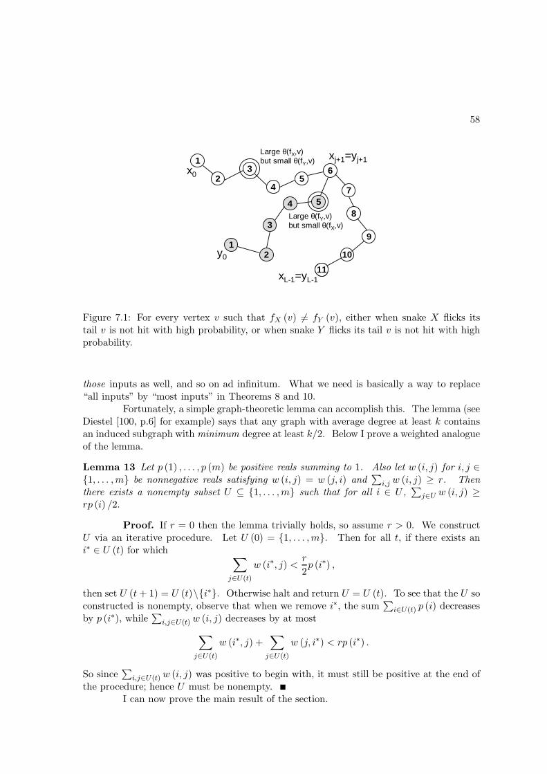
58

4

32

1

56

7

8

9

10

11

xj+1=yj+1

x0

54

3

21

11

y0

Large θ(fX,v) but small θ(fY,v)

Large θ(fY,v) but small θ(fX,v)

xL-1=yL-1

Figure 7.1: For every vertex v such that fX (v) 6= fY (v), either when snake X flicks itstail v is not hit with high probability, or when snake Y flicks its tail v is not hit with highprobability.

those inputs as well, and so on ad infinitum. What we need is basically a way to replace“all inputs” by “most inputs” in Theorems 8 and 10.

Fortunately, a simple graph-theoretic lemma can accomplish this. The lemma (seeDiestel [100, p.6] for example) says that any graph with average degree at least k containsan induced subgraph with minimum degree at least k/2. Below I prove a weighted analogueof the lemma.

Lemma 13 Let p (1) , . . . , p (m) be positive reals summing to 1. Also let w (i, j) for i, j ∈1, . . . ,m be nonnegative reals satisfying w (i, j) = w (j, i) and

∑i,j w (i, j) ≥ r. Then

there exists a nonempty subset U ⊆ 1, . . . ,m such that for all i ∈ U ,∑

j∈U w (i, j) ≥rp (i) /2.

Proof. If r = 0 then the lemma trivially holds, so assume r > 0. We constructU via an iterative procedure. Let U (0) = 1, . . . ,m. Then for all t, if there exists ani∗ ∈ U (t) for which ∑

j∈U(t)

w (i∗, j) <r

2p (i∗) ,

then set U (t+ 1) = U (t)\i∗. Otherwise halt and return U = U (t). To see that the U soconstructed is nonempty, observe that when we remove i∗, the sum

∑i∈U(t) p (i) decreases

by p (i∗), while∑

i,j∈U(t) w (i, j) decreases by at most

∑

j∈U(t)

w (i∗, j) +∑

j∈U(t)

w (j, i∗) < rp (i∗) .

So since∑

i,j∈U(t) w (i, j) was positive to begin with, it must still be positive at the end ofthe procedure; hence U must be nonempty.

I can now prove the main result of the section.

59

Theorem 14 Suppose a snake drawn from Dh,L is ε-good with probability at least 9/10.Then

RLS (G) = Ω (1/ε) , QLS (G) = Ω(√

1/ε).

Proof. Given a snake X ∈ Dh,L, we construct an input function fX as follows.For each v ∈ X, let fX (v) = min t : xt = v; and for each v /∈ X, let fX (v) = ∆ (v, h) +Lwhere ∆ (v, h) is the distance from v to h in G. Clearly fX so defined has a unique localminimum at x0. To obtain a decision problem, we stipulate that querying x0 reveals ananswer bit (0 or 1) in addition to fX (x1); the algorithm’s goal is then to return the answerbit. Obviously a lower bound for the decision problem implies a corresponding lower boundfor the search problem. Let us first prove the theorem in the case that all snakes in Dh,L areε-good. Let p (X) be the probability of drawing snake X from Dh,L. Also, given snakesX,Y and j ∈ 0, . . . , L− 1, let qj (X,Y ) be the probability that X∗ = Y , if X∗ is drawnfrom Dh,L conditioned on agreeing with X on all steps later than j. Then define

w (X,Y ) =p (X)

L

L−1∑

j=0

qj (X,Y ) .

The first claim is that w is symmetric; that is, w (X,Y ) = w (Y,X). It suffices to showthat

p (X) qj (X,Y ) = p (Y ) qj (Y,X)

for all j. We can assume X agrees with Y on all steps later than j, since otherwiseqj (X,Y ) = qj (Y,X) = 0. Given an X∗ ∈ Dh,L, let A denote the event that X∗ agreeswith X (or equivalently Y ) on all steps later than j, and let BX (resp. BY ) denote theevent that X∗ agrees with X (resp. Y ) on steps 1 to j. Then

p (X) qj (X,Y ) = Pr [A] Pr [BX |A] · Pr [BY |A]

= p (Y ) qj (Y,X) .

Now let E (X,Y ) denote the event that X ∩ Y = SX,Y , where SX,Y is as in Definition12. Also, let fX be the input obtained from X that has answer bit 0, and gX be theinput that has answer bit 1. To apply Theorems 8 and 10, take A = fX : X ∈ Dh,Land B = gX : X ∈ Dh,L. Then take R (fX , gY ) = w (X,Y ) if E (X,Y ) holds, andR (fX , gY ) = 0 otherwise. Given fX ∈ A and gY ∈ B with R (fX , gY ) > 0, and letting vbe a vertex such that fX (v) 6= gY (v), we must then have either v /∈ X or v /∈ Y . Supposethe former case; then

∑

fX∗∈A : fX∗(v) 6=gY (v)

R (fX∗ , gY ) ≤∑

fX∗∈A : fX∗(v) 6=gY (v)

p (Y )

L

L−1∑

j=0

qj (Y,X∗) ≤ εp (Y ) ,

since Y is ε-good. Thus θ (gY , v) equals

∑fX∗∈A : fX∗(v) 6=gY (v)R (fX∗ , gY )

∑fX∗∈AR (fX∗, gY )

≤ εp (Y )

9p (Y ) /10.

60

Similarly, if v /∈ Y then θ (fX , v) ≤ 10ε/9 by symmetry. Hence

υmin = maxfX∈A, gY ∈B, v : R(fX ,gY )>0, fX(v) 6=gY (v)

min θ (fX , v) , θ (gY , v) ≤ ε

9/10,

υgeom = maxfX∈A, gY ∈B, v : R(fX ,gY )>0, fX(v) 6=gY (v)

√θ (fX , v) θ (gY , v) ≤

√ε

9/10,

the latter since θ (fX , v) ≤ 1 and θ (gY , v) ≤ 1 for all fX , gY and v.In the general case, all we know is that a snake drawn from Dh,L is ε-good with

probability at least 9/10. Let G (X) denote the event that X is ε-good. Take A∗ =fX ∈ A : G (X) and B∗ = gY ∈ B : G (Y ), and take R (fX , gY ) as before. Then since

∑

X,Y : E(X,Y )

w (X,Y ) ≥∑

X

9

10p (X) ≥ 9

10,

by the union bound we have

∑

fX∈A∗, gY ∈B∗

R (fX , gY ) ≥∑

X,Y : G(X)∧G(Y )∧E(X,Y )

w (X,Y ) −∑

X : qG(X)

p (X) −∑

Y : qG(Y )

p (Y )

≥ 9

10− 1

10− 1

10

=7

10.

So by Lemma 13, there exist subsets A ⊆ A∗ and B ⊆ B∗ such that for all fX ∈ A andgY ∈ B,

∑

gY ∗∈B

R (fX , gY ∗) ≥ 7p (X)

20,

∑

fX∗∈A

R (fX∗, gY ) ≥ 7p (Y )

20.

So for all fX , gY with R (fX , gY ) > 0, and all v such that fX (v) 6= gY (v), either θ (fX , v) ≤20ε/7 or θ (gY , v) ≤ 20ε/7. Hence υmin ≤ 20ε/7 and υgeom ≤

√20ε/7.

7.5 Specific Graphs

In this section I apply the ‘snake method’ developed in Section 7.4 to specific examplesof graphs: the Boolean hypercube in Section 7.5.1, and the d-dimensional cubic grid (ford ≥ 3) in Section 7.5.2.

7.5.1 Boolean Hypercube

Abusing notation, let 0, 1n denote the n-dimensional Boolean hypercube—that is, thegraph whose vertices are n-bit strings, with two vertices adjacent if and only if they have

61

Hamming distance 1. Given a vertex v ∈ 0, 1n, let v [0] , . . . , v [n− 1] denote the nbits of v, and let v(i) denote the neighbor obtained by flipping bit v [i]. In this section Ilower-bound RLS (0, 1n) and QLS (0, 1n).

Fix a ‘snake head’ h ∈ 0, 1n and take L = 2n/2/100. I define the snake distribu-tion Dh,L via what I call a coordinate loop, as follows. Starting from x0 = h, for each t take

xt+1 = xt with 1/2 probability, and xt+1 = x(tmodn)t with 1/2 probability. The following is

a basic fact about this distribution.

Proposition 15 The coordinate loop mixes completely in n steps, in the sense that if t∗ ≥t+ n, then xt∗ is a uniform random vertex conditioned on xt.

One could also use the random walk distribution, following Aldous [24]. However,not only is the coordinate loop distribution easier to work with (since it produces fewerself-intersections), it also yields a better lower bound (since it mixes completely in n steps,as opposed to approximately in n log n steps).

I first upper-bound the probability, over X, j, and Y [j], that X∩Y 6= SX,Y (whereSX,Y is as in Definition 12).

Lemma 16 Suppose X is drawn from Dh,L, j is drawn uniformly from 0, . . . , L− 1, andY [j] is drawn from Dxj ,j. Then PrX,j,Y [j] [X ∩ Y = SX,Y ] ≥ 0.9999.

Proof. Call a disagreement a vertex v such that

min t : xt = v 6= min t∗ : yt∗ = v .

Clearly if there are no disagreements then X ∩ Y = SX,Y . If v is a disagreement, then bythe definition of Dh,L we cannot have both t > j−n and t∗ > j−n. So by Proposition 15,either yt∗ is uniformly random conditioned on X, or xt is uniformly random conditioned onY [j]. Hence PrX,j,Y [j] [xt = yt∗ ] = 1/2n. So by the union bound,

PrX,j,Y [j]

[X ∩ Y 6= SX,Y ] ≤ L2

2n= 0.0001.

I now argue that, unless X spends a ‘pathological’ amount of time in one part ofthe hypercube, the probability of any vertex v being hit when X flicks its tail is small. Toprove this, I define a notion of sparseness, and then show that (1) almost all snakes drawnfrom Dh,L are sparse (Lemma 18), and (2) sparse snakes are unlikely to hit any given vertexv (Lemma 19).

Definition 17 Given vertices v,w and i ∈ 0, . . . , n− 1, let ∆ (x, v, i) be the number ofsteps needed to reach v from x by first setting x [i] := v [i], then setting x [i− 1] := v [i− 1],and so on. (After we set x [0] we wrap around to x [n− 1].) Then X is sparse if thereexists a constant c such that for all v ∈ 0, 1n and all k,

|t : ∆ (xt, v, tmodn) = k| ≤ cn

(n+

L

2n−k

).

62

Lemma 18 If X is drawn from Dh,L, then X is sparse with probability 1 − o (1).

Proof. For each i ∈ 0, . . . , n− 1, the number of t ∈ 0, . . . , L− 1 such that

t ≡ i (modn) is at most L/n. For such a t, let E(v,i,k)t be the event that ∆ (xt, v, i) ≤ k;

then E(v,i,k)t holds if and only if

xt [i] = v [i] , . . . , xt [i− k + 1] = v [i− k + 1]

(where we wrap around to xt [n− 1] after reaching xt [0]). This occurs with probability

2k/2n over X. Furthermore, by Proposition 15, the E(v,i,k)t events for different t’s are

independent. So let

µk =L

n· 2k

2n;

then for fixed v, i, k, the expected number of t’s for which E(v,i,k)t holds is at most µk. Thus

by a Chernoff bound, if µk ≥ 1 then

PrX

[∣∣∣t : E

(v,i,k)t

∣∣∣ > cn · µk]<

(ecn−1

(cn)cn

)µk

<1

22n

for sufficiently large c. Similarly, if µk < 1 then

PrX

[∣∣∣t : E

(v,i,k)t

∣∣∣ > cn]<

(ecn/µk−1

(cn/µk)cn/µk

)µk

<1

22n

for sufficiently large c. By the union bound, then,

∣∣∣t : E

(v,i,k)t

∣∣∣ ≤ cn · (1 + µk)

= c

(n+

L

2n−k

)

for every v, i, k triple simultaneously with probability at least 1 − n22n/22n = 1 − o (1).Summing over all i’s produces the additional factor of n.

Lemma 19 If X is sparse, then for every v ∈ 0, 1n,

Prj,Y

[v ∈ Y [j]] = O

(n2

L

).

Proof. By assumption, for every k ∈ 0, . . . , n,

Prj

[∆ (xj, v, jmodn) = k] ≤ |t : ∆ (xt, v, tmodn) = k|L

≤ cn

L

(n+

L

2n−k

).

63

Consider the probability that v ∈ Y [j] in the event that ∆ (xj, v, jmodn) = k. Clearly

PrY

[v ∈ yj−n+1, . . . , yj] =1

2k.

Also, Proposition 15 implies that for every t ≤ j − n, the probability that yt = v is 2−n.So by the union bound,

PrY

[v ∈ y0, . . . , yj−n] ≤L

2n.

Then Prj,Y [v ∈ Y [j]] equals

n∑

k=0

(Prj [∆ (xj, v, jmodn) = k] ·

PrY [v ∈ Y [j] | ∆ (xj, v, jmodn) = k]

)≤

n∑

k=0

cn

L

(n+

L

2n−k

)(1

2k+L

2n

)

= O

(cn2

L

)

as can be verified by breaking the sum into cases and doing some manipulations.The main result follows easily:

Theorem 20

RLS (0, 1n) = Ω

(2n/2

n2

), QLS (0, 1n) = Ω

(2n/4

n

).

Proof. Take ε = n2/2n/2. Then by Theorem 14, it suffices to show that a snakeX drawn from Dh,L is O (ε)-good with probability at least 9/10. First, since

PrX,j,Y [j]

[X ∩ Y = SX,Y ] ≥ 0.9999

by Lemma 16, Markov’s inequality shows that

PrX

[Prj,Y [j]

[X ∩ Y = SX,Y ] ≥ 9

10

]≥ 19

20.

Second, by Lemma 18, X is sparse with probability 1 − o (1), and by Lemma 19, if X issparse then

Prj,Y

[v ∈ Y [j]] = O

(n2

L

)= O (ε)

for every v. So both requirements of Definition 12 hold simultaneously with probability atleast 9/10.

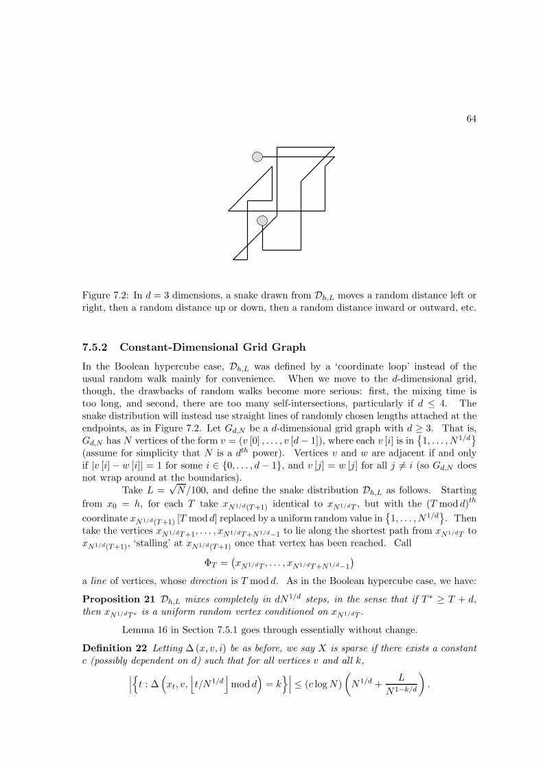
64

Figure 7.2: In d = 3 dimensions, a snake drawn from Dh,L moves a random distance left orright, then a random distance up or down, then a random distance inward or outward, etc.

7.5.2 Constant-Dimensional Grid Graph

In the Boolean hypercube case, Dh,L was defined by a ‘coordinate loop’ instead of theusual random walk mainly for convenience. When we move to the d-dimensional grid,though, the drawbacks of random walks become more serious: first, the mixing time istoo long, and second, there are too many self-intersections, particularly if d ≤ 4. Thesnake distribution will instead use straight lines of randomly chosen lengths attached at theendpoints, as in Figure 7.2. Let Gd,N be a d-dimensional grid graph with d ≥ 3. That is,Gd,N has N vertices of the form v = (v [0] , . . . , v [d− 1]), where each v [i] is in

1, . . . , N1/d

(assume for simplicity that N is a dth power). Vertices v and w are adjacent if and onlyif |v [i] − w [i]| = 1 for some i ∈ 0, . . . , d− 1, and v [j] = w [j] for all j 6= i (so Gd,N doesnot wrap around at the boundaries).

Take L =√N/100, and define the snake distribution Dh,L as follows. Starting

from x0 = h, for each T take xN1/d(T+1) identical to xN1/dT , but with the (T mod d)th

coordinate xN1/d(T+1) [T mod d] replaced by a uniform random value in1, . . . , N1/d

. Then

take the vertices xN1/dT+1, . . . , xN1/dT+N1/d−1 to lie along the shortest path from xN1/dT toxN1/d(T+1), ‘stalling’ at xN1/d(T+1) once that vertex has been reached. Call

ΦT =(xN1/dT , . . . , xN1/dT+N1/d−1

)

a line of vertices, whose direction is T mod d. As in the Boolean hypercube case, we have:

Proposition 21 Dh,L mixes completely in dN1/d steps, in the sense that if T ∗ ≥ T + d,then xN1/dT ∗ is a uniform random vertex conditioned on xN1/dT .

Lemma 16 in Section 7.5.1 goes through essentially without change.

Definition 22 Letting ∆ (x, v, i) be as before, we say X is sparse if there exists a constantc (possibly dependent on d) such that for all vertices v and all k,

∣∣∣t : ∆

(xt, v,

⌊t/N1/d

⌋mod d

)= k

∣∣∣ ≤ (c logN)

(N1/d +

L

N1−k/d

).

65

Lemma 23 If X is drawn from Dh,L, then X is sparse with probability 1 − o (1).

Proof. Similar to Lemma 18. Let ΦT be a line of vertices with direction i =T mod d, and notice that ∆ (xt, v, i) is the same for every vertex xt in ΦT . Let E

(v,i,k)T

denote the event that ∆ (xt, v, i) ≤ k for the xt’s in ΦT . Then E(v,i,k)T occurs with probability

N (k−1)/d/N over X. Furthermore, if |T − T ∗| ≥ d then E(v,i,k)T and E

(v,i,k)T ∗ are independent

events. So let

µk = L · N(k−1)/d

N;

then for fixed v, i, k, the expected number of lines for which E(v,i,k)T holds is at most µk.

Thus, by a Chernoff bound, if µk ≥ 1 then

PrX

[∣∣∣T : E

(v,i,k)T

∣∣∣ > c logN · µk]<

(ec logN−1

(c logN)c logN

)µk

which is at most 1/N2 for sufficiently large c. Similarly, if µk < 1 then letting m =(c logN) /µk,

PrX

[∣∣∣T : E

(v,i,k)T

∣∣∣ > c logN]<

(em−1

mm

)µk

<1

N2

for sufficiently large c. So with probability 1 − o (1) it holds that for all v, k, lettingit =

⌊t/N1/d

⌋mod d,

|t : ∆ (xt, v, it) = k| ≤ c logN · (1 + µk) ·N1/d

= (c logN)

(N1/d +

L

N1−k/d

).

Lemma 24 If X is sparse, then for every v ∈ Gd,N ,

Prj,Y

[v ∈ Y [j]] = O

(N1/d logN

L

),

where the big-O hides a constant dependent on d.

Proof. As in Lemma 19, setting ij =⌊j/N1/d

⌋mod d we obtain that Prj,Y [v ∈ Y [j]]

equals

d∑

k=1

Prj

[∆ (xj , v, ij) = k] PrY

[v ∈ Y [j] | ∆ (xj, v, ij) = k]

≤d∑

k=1

c logN

L

(N1/d +

L

N1−k/d

)(1

N (k−1)/d+L

N

)

= O

(N1/d logN

L

).

66

By the same proof as for Theorem 20, taking ε = (logN) /N1/2−1/d yields thefollowing:

Theorem 25 Neglecting a constant dependent on d, for all d ≥ 3

RLS (Gd,N ) = Ω

(N1/2−1/d

logN

),

QLS (Gd,N ) = Ω

√N1/2−1/d

logN

.

67

Chapter 8

Quantum Certificate Complexity

This chapter studies the relationships between classical and quantum measures ofquery complexity. Let f : S → 0, 1 be a Boolean function with S ⊆ 0, 1n, that takesinput Y = y1 . . . yn. Then the deterministic query complexity D (f) is the minimum numberof queries to the yi’s needed to evaluate f , if Y is chosen adversarially and if queries canbe adaptive (that is, can depend on the outcomes of previous queries). Also, the bounded-error randomized query complexity, R2 (f), is the minimum expected number of queriesneeded by a randomized algorithm that, for each Y , outputs f (Y ) with probability at least2/3. Here the ‘2’ refers to two-sided error; if instead we require f (Y ) to be output withprobability 1 for every Y , we obtain R0 (f), or zero-error randomized query complexity.

Analogously, Q2 (f) is the minimum number of queries needed by a quantumalgorithm that outputs f (Y ) with probability at least 2/3 for all Y . Also, for k ∈ 0, 1let Qk

0 (f) be the minimum number of queries needed by a quantum algorithm that outputsf (Y ) with probability 1 if f (Y ) = k, and with probability at least 1/2 if f (Y ) 6= k.Then let Q0 (f) = max

Q0

0 (f) ,Q10 (f)

. If we require a single algorithm that succeeds

with probability 1 for all Y , we obtain QE (f), or exact quantum query complexity. SeeBuhrman and de Wolf [78] for a more detailed survey of these measures.

It is immediate that

Q 2 (f) ≤ R 2 (f) ≤ R 0 (f) ≤ D(f) ≤ n,

that Q0 (f) ≤ R0 (f), and that QE (f) ≤ D (f). If f is partial (i.e. S 6= 0, 1n), then Q2 (f)can be superpolynomially smaller than R2 (f); this is what makes Shor’s period-findingalgorithm [221] possible. For total f , by contrast, the largest known gap even betweenD (f) and Q2 (f) is quadratic, and is achieved by the OR function on n bits: D (OR) = n(indeed R2 (OR) = Ω (n)), whereas Q2 (OR) = Θ (

√n) because of Grover’s search algorithm

[141]. Furthermore, for total f , Beals et al. [45] showed that D (f) = O(Q2 (f)6

), while

de Wolf [244] showed that D (f) = O(Q2 (f)2 Q0 (f)2

).

The result of Beals et al. [45] relies on two intermediate complexity measures, thecertificate complexity C (f) and block sensitivity bs (f), which are defined as follows.

Definition 26 A certificate for an input X is a set S ⊆ 1, . . . , n such that for all inputs

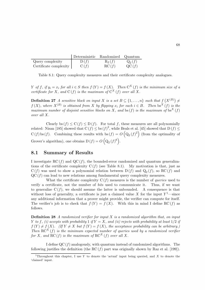
68

Deterministic Randomized Quantum

Query complexity D (f) R2 (f) Q2 (f)Certificate complexity C (f) RC (f) QC (f)

Table 8.1: Query complexity measures and their certificate complexity analogues.

Y of f , if yi = xi for all i ∈ S then f (Y ) = f (X). Then CX (f) is the minimum size of acertificate for X, and C (f) is the maximum of CX (f) over all X.

Definition 27 A sensitive block on input X is a set B ⊆ 1, . . . , n such that f(X(B)

)6=

f (X), where X(B) is obtained from X by flipping xi for each i ∈ B. Then bsX (f) is themaximum number of disjoint sensitive blocks on X, and bs (f) is the maximum of bsX (f)over all X.

Clearly bs (f) ≤ C(f) ≤ D (f). For total f , these measures are all polynomiallyrelated: Nisan [185] showed that C (f) ≤ bs (f)2, while Beals et al. [45] showed that D (f) ≤C (f) bs (f). Combining these results with bs (f) = O

(Q2 (f)2

)(from the optimality of

Grover’s algorithm), one obtains D (f) = O(Q2 (f)6

).

8.1 Summary of Results

I investigate RC (f) and QC (f), the bounded-error randomized and quantum generaliza-tions of the certificate complexity C (f) (see Table 8.1). My motivation is that, just asC (f) was used to show a polynomial relation between D (f) and Q2 (f), so RC (f) andQC (f) can lead to new relations among fundamental query complexity measures.

What the certificate complexity C (f) measures is the number of queries used toverify a certificate, not the number of bits used to communicate it. Thus, if we wantto generalize C (f), we should assume the latter is unbounded. A consequence is thatwithout loss of generality, a certificate is just a claimed value X for the input Y 1—sinceany additional information that a prover might provide, the verifier can compute for itself.The verifier’s job is to check that f (Y ) = f (X). With this in mind I define RC (f) asfollows.

Definition 28 A randomized verifier for input X is a randomized algorithm that, on inputY to f , (i) accepts with probability 1 if Y = X, and (ii) rejects with probability at least 1/2 iff (Y ) 6= f (X). (If Y 6= X but f (Y ) = f (X), the acceptance probability can be arbitrary.)Then RCX (f) is the minimum expected number of queries used by a randomized verifierfor X, and RC (f) is the maximum of RCX (f) over all X.

I define QC (f) analogously, with quantum instead of randomized algorithms. Thefollowing justifies the definition (the RC (f) part was originally shown by Raz et al. [199]).

1Throughout this chapter, I use Y to denote the ‘actual’ input being queried, and X to denote the‘claimed’ input.

69

Proposition 29 Making the error probability two-sided rather than one-sided changes RC (f)and QC(f) by at most a constant factor.

Proof. For RC (f), let rYV be the event that verifier V rejects on input Y , andlet dYV be the event that V encounters a disagreement with X on Y . We may assumePr[rYV | dYV

]= 1. Suppose that Pr

[rYV]≤ ε0 if Y = X and Pr

[rYV]≥ 1 − ε1 if f (Y ) 6=

f (X). We wish to lower-bound Pr[dYV]

for all Y such that f (Y ) 6= f (X). Observe that

Pr[rYV ∧ qdYV | f (Y ) 6= f (X)

]≤ Pr

[rXV ∧ qdXV

]= Pr

[rXV]≤ ε0.

Hence for f (Y ) 6= f (X),

Pr[dYV]≥ Pr

[rYV]− Pr

[rYV ∧ qdYV

]≥ 1 − ε1 − ε0.

Now let V ∗ be identical to V except that, whenever V rejects despite having found nodisagreement with X, V ∗ accepts. Clearly Pr

[rXV ∗]

= 0. Also, in the case f (Y ) 6= f (X),

Pr[rYV ∗]

= Pr[dYV]≥ 1 − ε1 − ε0.

The result follows since O (1) repetitions suffice to boost any constant error probability toany other constant error probability.

For QC(f), suppose the verifier’s final state given input Y is

∑

z

αYz |z〉(βYz |0〉 + γYz |1〉

)

where |0〉 is the reject state, |1〉 is the accept state, and∣∣βYz

∣∣2 +∣∣γYz∣∣2 = 1 for all z. Suppose

also that AX ≥ 1− ε0 and that AY ≤ ε1 whenever f (Y ) 6= f (X), where AY =∑

z

∣∣αYz γYz∣∣2

is the probability of accepting. Then the verifier can make AX = 1 by performing theconditional rotation (

γXz −βXzβXz γXz

)

on the second register prior to measurement. In the case f (Y ) 6= f (X), this produces

AY =∑

z

∣∣αYz∣∣2 ∣∣βXz βYz + γXz γ

Yz

∣∣2

≤ 2∑

z

∣∣αYz∣∣2(∣∣βXz

∣∣2 +∣∣γYz∣∣2)

≤ 2 (ε0 + ε1) .

It is immediate that QC (f) ≤ RC (f) ≤ C (f), that QC (f) = O (Q2 (f)), andthat RC (f) = O (R2 (f)). We also have RC (f) = Ω (bs (f)), since a randomized verifierfor X must query each sensitive block on X with 1/2 probability. This suggests viewingRC (f) as an ‘alloy’ of block sensitivity and certificate complexity, an interpretation forwhich Section 8.5 gives some justification.

70

The results of this chapter are as follows. In Section 8.3 I show that QC (f) =

Θ(√

RC (f))

for all f (partial or total), precisely characterizing quantum certificate com-

plexity in terms of randomized certificate complexity. To do this, I first give a nonadaptivecharacterization of RC (f), and then apply the adversary method of Ambainis [27] to lower-bound QC(f) in terms of this characterization. Then, in Section 8.4, I extend results onpolynomials due to de Wolf [244] and to Nisan and Smolensky (as described by Buhrmanand de Wolf [78]), to show that R0 (f) = O (RC (f) ndeg (f) log n) for all total f , wherendeg (f) is the minimum degree of a polynomial p such that p (X) 6= 0 if and only iff (X) 6= 0. Combining the results of Sections 8.3 and 8.4 leads to a new lower bound on

quantum query complexity: that R0 (f) = O(Q2 (f)2 Q0 (f) log n

)for all total f . To my

knowledge, this is the first quantum lower bound to use both the adversary method andthe polynomial method at different points in the argument.

Finally, in Section 8.5, I exhibit asymptotic gaps between RC (f) and other query

complexity measures, including a total f for which C (f) = Θ(QC (f)2.205

), and a sym-

metric partial f for which QC (f) = O (1) yet Q2 (f) = Ω (n/ log n). I conclude in Section8.6 with some open problems.

8.2 Related Work

Raz et al. [199] studied a query complexity measure they called ma (f), for Merlin-Arthur.In my notation, ma (f) equals the maximum of RCX (f) over all X with f (X) = 1. Razet al. observed that ma (f) = ip (f), where ip (f) is the number of queries needed givenarbitrarily many rounds of interaction with a prover. They also used error-correcting codesto construct a total f for which ma (f) = O (1) but C (f) = Ω (n). This has similarities tothe construction, in Section 8.5.2, of a symmetric partial f for which QC(f) = O (1) butQ2 (f) = Ω (n/ log n). Aside from that and from Proposition 29, Raz et al.’s results do notoverlap with the results here.

Watrous [239] has investigated a different notion of ‘quantum certificate complexity’—whether certificates that are quantum states can be superpolynomially smaller than anyclassical certificate. Also, de Wolf [245] has investigated ‘nondeterministic quantum querycomplexity’ in the alternate sense of algorithms that accept with zero probability whenf (Y ) = 0, and with positive probability when f (Y ) = 1.

8.3 Characterization of Quantum Certificate Complexity

We wish to show that QC(f) = Θ(√

RC (f)), precisely characterizing quantum certificate

complexity in terms of randomized certificate complexity. The first step is to give a simplercharacterization of RC (f).

Lemma 30 Call a randomized verifier for X nonadaptive if, on input Y , it queries eachyi with independent probability λi, and rejects if and only if it encounters a disagreementwith X. (Thus, we identify such a verifier with the vector (λ1, . . . , λn).) Let RCX

na (f)

71

be the minimum of λ1 + · · · + λn over all nonadaptive verifiers for X. Then RCXna (f) =

Θ(RCX (f)

).

Proof. Clearly RCXna (f) = Ω

(RCX (f)

). For the upper bound, we can assume

that a randomized verifier rejects immediately on finding a disagreement with X, andaccepts if it finds no disagreement. Let Y = Y : f (Y ) 6= f (X). Let V be an optimalrandomized verifier, and let pt (Y ) be the probability that V , when given input Y ∈ Y, findsa disagreement with X on the tth query. By Markov’s inequality, V must have found adisagreement with probability at least 1/2 after T =

⌈2RCX (f)

⌉queries. So by the union

bound

p1 (Y ) + · · · + pT (Y ) ≥ 1

2

for each Y ∈ Y. Suppose we choose t ∈ 1, . . . , T uniformly at random and simulate thetth query, pretending that queries 1, . . . , t − 1 have already been made and have returnedagreement with X. Then we must find a disagreement with probability at least 1/2T .By repeating this procedure 4T times, we can boost the probability to 1 − e−2. For i ∈1, . . . , n, let λi be the probability that yi is queried at least once. Then λ1+· · ·+λn ≤ 4T ,whereas for each Y ∈ Y, ∑

i:yi 6=xi

λi ≥ 1 − e−2.

It follows that, if each yi is queried with independent probability λi, then the probabilitythat at least one yi disagrees with X is at least

1 −∏

i:yi 6=xi

(1 − λi) ≥ 1 −(

1 − 1 − e−2

n

)n> 0.57.

To obtain a lower bound on QC(f), I will use the following simple reformulationof Ambainis’s adversary method [27].

Theorem 31 (Ambainis) Given a function f : S → 0, 1 with S ⊆ 0, 1n, let β bea function from S to nonnegative reals, and let R : S2 → 0, 1 be a relation such thatR (X,Y ) = R (Y,X) for all X,Y and R (X,Y ) = 0 whenever f (X) = f (Y ). Let δ0, δ1 ∈(0, 1] be such that for every X ∈ S and i ∈ 1, . . . , n,

∑

Y :R(X,Y )=1

β (Y ) ≥ 1,

∑

Y :R(X,Y )=1,xi 6=yi

β (Y ) ≤ δf(X).

Then Q2 (f) = Ω(√

1δ0δ1

).

I now prove the main result of the section.

72

Theorem 32 For all f (partial or total) and all X,

QCX (f) = Θ

(√RCX (f)

).

Proof. Let (λ1, . . . , λn) be an optimal nonadaptive randomized verifier for X, andlet

S = λ1 + · · · + λn.

First, QCX (f) = O(√

S). We can run a “weighted Grover search,” in which the propor-

tion of basis states querying index i is within a constant factor of λi/S. (It suffices to use

n2 basis states.) Let Y = Y : f (Y ) 6= f (X); then for any Y ∈ Y, O(√

S)

iterations

suffice to find a disagreement with X with probability Ω (1). Second, QCX (f) = Ω(√

S).

Consider a matrix game in which Alice chooses an index i to query and Bob chooses Y ∈ Y;Alice wins if and only if yi 6= xi. If both players are rational, then Alice wins with proba-bility O (1/S), since otherwise Alice’s strategy would yield a verifier (λ′1, . . . , λ

′n) with

λ′1 + · · · + λ′n = o (S) .

Hence by the minimax theorem, there exists a distribution µ over Y such that for every i,

PrY ∈µ

[yi 6= xi] = O

(1

S

).

Let β (X) = 1 and let β (Y ) = µ (Y ) for each Y ∈ Y. Also, let R (Y,Z) = 1 if and onlyif Z = X for each Y ∈ Y and Z /∈ Y. Then we can take δf(Y ) = 1 and δf(X) = O (1/S)in Theorem 31. So the quantum query complexity of distinguishing X from an arbitrary

Y ∈ Y is Ω(√

S).

8.4 Quantum Lower Bound for Total Functions

The goal of this section is to show that

R0 (f) = O(Q2 (f)2 Q0 (f) log n

)

for all total f . Say that a real multilinear polynomial p (x1, . . . , xn) nondeterministicallyrepresents f if for all X ∈ 0, 1n, p (X) 6= 0 if and only if f (X) 6= 0. Let ndeg (f) be theminimum degree of a nondeterministic polynomial for f . Also, given such a polynomial p,say that a monomial M1 ∈ p is covered by M2 ∈ p if M2 contains every variable in M1. Amonomial M is called a maxonomial if it is not covered by any other monomial of p. Thefollowing is a simple generalization of a lemma attributed in [78] to Nisan and Smolensky.

Lemma 33 (Nisan-Smolensky) Let p nondeterministically represent f . Then for everymaxonomial M of p and X ∈ f−1 (0), there is a set B of variables in M such that f

(X(B)

)6=

f (X), where X(B) is obtained from X by flipping the variables in B.

73

Proof. Obtain a restricted function g from f , and a restricted polynomial q fromp, by setting each variable outside of M to xi. Then g cannot be constant, since itsrepresenting polynomial q contains M as a monomial. Thus there is a subset B of variablesin M such that g

(X(B)

)= 1, and hence f

(X(B)

)= 1.

Using Lemma 33, de Wolf [244] showed that D (f) ≤ C (f) ndeg (f) for all totalf , slightly improving the result D (f) ≤ C (f) deg (f) due to Buhrman and de Wolf [78].In Theorem 35, I will give an analogue of this result for randomized query and certificatecomplexities. However, I first need a probabilistic lemma.

Lemma 34 Suppose we repeatedly apply the following procedure: first identify the set B ofmaxonomials of p, then ‘shrink’ each M ∈ B with (not necessarily independent) probabilityat least 1/2. Shrinking M means replacing it by an arbitrary monomial of degree deg (M)−1. Then with high probability p is a constant polynomial after O (deg (p) log n) iterations.

Proof. For any set A of monomials, consider the weighting function

ω (A) =∑

M∈Adeg (M)!

Let S be the set of monomials of p. Initially ω (S) ≤ ndeg(p) deg (p)!, and we are done whenω (S) = 0. The claim is that at every iteration, ω (B) ≥ 1

eω (S). For every M∗ ∈ S \B is

covered by some M ∈ B, but a given M ∈ B can cover at most(deg(M)

`

)distinct M∗ with

deg (M∗) = `. Hence

ω (S \B) ≤∑

M∈B

deg(M)−1∑

`=0

(deg(M)`

)`!

≤∑

M∈Bdeg (M)!

(1

1!+

1

2!+ · · ·

)

≤ (e− 1)ω (B) .

At every iteration, the contribution of each M ∈ B to ω (A) has at least 1/2probability of shrinking from deg (M)! to (deg (M) − 1)! (or to 0 if deg (M) = 1). Whenthis occurs, the contribution of M is at least halved. Hence ω (S) decreases by an expectedamount at least 1

4eω (S). Thus after

log4e/(4e−1)

(2ndeg(p) deg (p)!

)= O (deg (p) log n)

iterations, the expectation of ω (S) is less than 1/2, so S is empty with probability at least1/2.

I can now prove the main result.2

Theorem 35 For total f ,

R0 (f) = O (RC (f) ndeg (f) log n) .

2The proof of Theorem 35 that I gave previously [4] makes a claim that is both superfluous for provingthe theorem and false. I am grateful to Gatis Midrijanis for pointing this out to me.

74

Proof. The algorithm is as follows.

Repeat

Choose a 0-input X compatible with all queries made so far3

Query a randomized 0-certificate for X

Until f has been restricted to a constant function

Let p be a polynomial that nondeterministically represents f . Then the key factis that for every 0-input X, when we query a randomized 0-certificate for X we “hit” eachmaxonomial M of p with probability at least 1/2. Here hitting M means querying avariable in M . This is because, by Lemma 33, it is possible to change f (X) from 0 to 1just by flipping variables in M . So a randomized certificate would be incorrect if it probedthose variables with probability less than 1/2.

Therefore, each iteration of the algorithm shrinks each maxonomial of p withprobability at least 1/2. It follows from Lemma 34 that the algorithm terminates after anexpected number of iterations O (deg (p) log n).

Buhrman et al. [45] showed that ndeg (f) ≤ 2Q0 (f). Combining this with Theo-rems 32 and 35 yields a new relation between classical and quantum query complexity.

Corollary 36 For all total f ,

R0 (f) = O(Q2 (f)2 Q0 (f) log n

).

The best previous relation of this kind was R0 (f) = O(Q2 (f)2 Q0 (f)2

), due to

de Wolf [244]. It is worth mentioning another corollary of Theorems 32 and 35, this onepurely classical:

Corollary 37 For all total f ,

R0 (f) = O (R2 (f) ndeg (f) log n)

Previously, no relation between R0 and R2 better than R0 (f) = O(R2 (f)3

)was

known (although no asymptotic gap between R0 and R2 is known either [212]).

8.5 Asymptotic Gaps

Having related RC (f) and QC (f) to other query complexity measures in Section 8.4, inwhat follows I seek the largest possible asymptotic gaps among the measures. In particular,

I give a total f for which RC (f) = Θ(C (f)0.907

)and hence C (f) = Θ

(QC (f)2.205

), as

well as a total f for which bs (f) = Θ(RC (f)0.922

). Although these gaps are the largest

3Clearly, as long as f is not a constant function, there exists a 0-input X compatible with all queriesmade so far.

75

of which I know, Section 8.5.1 shows that no ‘local’ technique can improve the relations

C (f) = O(RC (f)2

)and RC (f) = O

(bs (f)2

). Finally, Section 8.5.2 uses combinatorial

designs to construct a symmetric partial f for which RC (f) and QC (f) are O (1), yetQ2 (f) = Ω (n/ log n).

Wegener and Zadori [240] exhibited total Boolean functions with asymptotic gapsbetween C (f) and bs (f). In similar fashion, I give a function family gt with an asymp-totic gap between C (gt) and RC (gt). Let g1 (x1, . . . , x29) equal 1 if and only if the Hammingweight of its input is 13, 14, 15, or 16. (The parameter 29 was found via computer searchto produce a maximal separation.) Then for t > 1, let

gt (x1, . . . , x29t) = g0 [gt−1 (X1) , . . . , gt−1 (X29)]

where X1 is the first 29t−1 input bits, X2 is the second 29t−1, and so on. For k ∈ 0, 1,let

bs k (f) = maxf(X)=k

bsX (f) ,

C k (f) = maxf(X)=k

CX (f) .

Then since bs0 (g1) = bs1 (g1) = 17, we have bs (gt) = 17t. On the other hand, C0 (g1) = 17but C1 (g1) = 26, so

C 1 (gt) = 13C 1 (gt−1) + 13C 0 (gt−1) ,

C 0 (gt) = 17maxC 1 (gt−1) ,C

0 (gt−1).

Solving this recurrence yields C (gt) = Θ(22.725t

). We can now show a gap between C

and RC.

Proposition 38 RC (gt) = Θ(C (gt)

0.907).

Proof. Since bs (gt) = Ω(C (gt)

0.907), it suffices to show that RC (gt) = O (bs (gt)).

The randomized verifier V chooses an input variable to query as follows. Let X bethe claimed input, and let K =

∑29i=1 gt−1 (Xi). Let I0 = i : gt−1 (Xi) = 0 and I1 =

i : gt−1 (Xi) = 1. With probability pK , V chooses an i ∈ I1 uniformly at random; other-wise A chooses an i ∈ I0 uniformly at random. Here pK is as follows.

K [0, 12] 13 14 15 16 [17, 29]

pK 0 1317

712

512

417 1

Once i is chosen, V repeats the procedure for Xi, and continues recursively in thismanner until reaching a variable yj to query. One can check that if gt (X) 6= gt (Y ), thengt−1 (Xi) 6= gt−1 (Yi) with probability at least 1/17. Hence xj 6= yj with probability atleast 1/17t, and RC (gt) = O

(17t).

By Theorem 32, it follows that C (gt) = Θ(QC (gt)

2.205). This offers a surpris-

ing contrast with the query complexity setting, where the best known gap between the

deterministic and quantum measures is quadratic (D (f) = Θ(Q2 (f)2

)).

76

The family gt happens not to yield an asymptotic gap between bs (f) and RC (f).The reason is that any input to g0 can be covered perfectly by sensitive blocks of minimumsize, with no variables left over. In general, though, one can have bs (f) = o (RC (f)). Asreported by Bublitz et al. [74], M. Paterson found a total Boolean function h1 (x1, . . . , x6)such that CX (h1) = 5 and bsX (h1) = 4 for all X. Composing h1 recursively yields

bs (ht) = Θ(C(ht)

0.861)

and bs (ht) = Θ(RC (ht)

0.922), both of which are the largest such

gaps of which I know.

8.5.1 Local Separations

It is a longstanding open question whether the relation C (f) ≤ bs (f)2 due to Nisan [185]

is tight. As a first step, one can ask whether the relations C (f) = O(RC (f)2

)and

RC (f) = O(bs (f)2

)are tight. In this section I introduce a notion of local proof in query

complexity, and then show there is no local proof that C (f) = o(RC (f)2

)or that RC (f) =

o(bs (f)2

). This implies that proving either result would require techniques unlike those

that are currently known. My inspiration comes from computational complexity, whereresearchers first formalized known methods of proof, including relativizable proofs [41] andnatural proofs [202], and then argued that these methods were not powerful enough toresolve the field’s outstanding problems.

Let G (f) and H (f) be query complexity measures obtained by maximizing overall inputs—that is,

G (f) = maxX

GX (f) ,

H (f) = maxX

HX (f) .

Call B ⊆ 1, . . . , n a minimal block on X if B is sensitive on X (meaning f(X(B)

)6=

f (X)), and no sub-block B′ ⊂ B is sensitive on X. Also, let X’s neighborhood N (X)consist of X together with X(B) for every minimal block B of X. Consider a proof thatG (f) = O (t (H (f))) for some nondecreasing t. I call the proof local if it proceeds byshowing that for every input X,

GX (f) = O

(max

Y ∈N (X)

t(HY (f)

)).

As a canonical example, Nisan’s proof [185] that C (f) ≤ bs (f)2 is local. For each X,Nisan observes that (i) a maximal set of disjoint minimal blocks is a certificate for X, (ii)such a set can contain at most bsX (f) blocks, and (iii) each block can have size at mostmaxY ∈N (X) bsY (f). Another example of a local proof is the proof in Section 8.3 that

RC (f) = O(QC(f)2

).

Proposition 39 There is no local proof showing that C (f) = o(RC (f)2

)or that RC (f) =

o(bs (f)2

)for all total f .

77

Proof. The first part is easy: let f (X) = 1 if |X| ≥ √n (where |X| denotes the

Hamming weight of X), and f (X) = 0 otherwise. Consider the all-zero input 0n. Wehave C0n

(f) = n−d√ne+1, but RC0n(f) = O (

√n), and indeed RCY (f) = O (

√n) for all

Y ∈ N (0n). For the second part, arrange the input variables in a lattice of size√n×√

n.Take m = Θ

(n1/3

), and let g (X) be the monotone Boolean function that outputs 1 if and

only if X contains a 1-square of size m×m. This is a square of 1’s that can wrap aroundthe edges of the lattice; note that only the variables along the sides must be set to 1, notthose in the interior. An example input, with a 1-square of size 3 × 3, is shown below.

0 0 0 0 00 0 0 0 01 0 0 1 11 0 0 1 01 0 0 1 1

Clearly bs0n

(g) = Θ(n1/3

), since there can be at most n/m2 disjoint 1-squares of size

m×m. Also, bsY (g) = Θ(n1/3

)for any Y that is 0 except for a single 1-square. On the

other hand, if we choose uniformly at random among all such Y ’s, then at any lattice sitei, PrY [yi = 1] = Θ

(n−2/3

). Hence RC0n

(g) = Ω(n2/3

).

8.5.2 Symmetric Partial Functions

If f is partial, then QC (f) can be much smaller than Q2 (f). This is strikingly illustratedby the collision problem: let Col (Y ) = 0 if Y = y1 . . . yn is a one-to-one sequence andCol (Y ) = 1 if Y is a two-to-one sequence, promised that one of these is the case. ThenRC (Col) = QC (Col) = O (1), since every one-to-one input differs from every two-to-oneinput on at least n/2 of the yi’s. On the other hand, Chapter 6 showed that Q2 (Col) =Ω(n1/5

).From the example of the collision problem, it is tempting to conjecture that (say)

Q2 (f) = O(n1/3

)whenever QC(f) = O (1)—that is, ‘if every 0-input is far from every

1-input, then the quantum query complexity is sublinear.’ Here I disprove this conjecture,even for the special case of symmetric functions such as Col. (Given a finite set H, a functionf : S → 0, 1 where S ⊆ Hn is called symmetric if x1 . . . xn ∈ S implies xσ(1) . . . xσ(n) ∈ Sand f (x1 . . . xn) = f

(xσ(1) . . . xσ(n)

)for every permutation σ.)

The proof uses the following lemma, which can be found in Nisan and Wigderson[187] for example.

Lemma 40 (Nisan-Wigderson) For any γ > 1, there exists a family of sets

A1, . . . , Am ⊆ 1, . . . , dγne

such that m = Ω(2n/γ

), |Ai| = n for all i, and |Ai ∩Aj| ≤ n/γ for all i 6= j.

A lemma due to Ambainis [26] is also useful. Let f : S → 0, 1 where S ⊆0, 1n be a partial Boolean function, and let p : 0, 1n → R be a real-valued multilinearpolynomial. We say that p approximates f if (i) p (X) ∈ [0, 1] for every input X ∈ 0, 1n(not merely those in S), and (ii) |p (X) − g (X)| ≤ 1/3 for every X ∈ S.

78

Lemma 41 (Ambainis) At most 2O(∆(n,d)dn2) distinct Boolean functions (partial or total)can be approximated by polynomials of degree d, where ∆ (n, d) =

∑di=0

(ni

).

The result is an easy consequence of Lemmas 40 and 41.

Theorem 42 There exists a symmetric partial f for which QC(f) = O (1) and Q2 (f) =Ω (n/ log n).

Proof. Let f : S → 0, 1 where S ⊆ 1, . . . , 3nn, and let m = Ω(2n/3

).

Let A1, . . . , Am ⊆ 1, . . . , 3n be as in Lemma 40. We put x1, . . . , xn in S if and only ifx1, . . . , xn = Aj for some j. Clearly QC(f) = O (1), since if i 6= j then every permutationof Ai differs from every permutation of Aj on at least n/3 indices. The number of symmetric

f with S as above is 2m = 2Ω(2n/3). We can convert any such f to a Boolean functiong on O (n log n) variables. But Beals et al. [45] showed that, if Q2 (g) = T , then g isapproximated by a polynomial of degree at most 2T . So by Lemma 41, if Q2 (g) ≤ T forevery g then

2T · ∆ (n log n, 2T ) · (n log n)2 = Ω(2n/3

)

and we solve to obtain T = Ω (n/ log n).

8.6 Open Problems

Is deg (f) = Ω(√

RC (f)), where deg (f) is the minimum degree of a polynomial approx-

imating f? In other words, can one lower-bound QC (f) using the polynomial method ofBeals et al. [45], rather than the adversary method of Ambainis [27]?

Also, is R0 (f) = O(RC (f)2

)? If so we obtain the new relations R0 (f) =

O(Q2 (f)4

)and R0 (f) = O

(R2 (f)2

).

79

Chapter 9

The Need to Uncompute

Like a classical algorithm, a quantum algorithm can solve problems recursively bycalling itself as a subroutine. When this is done, though, the algorithm typically needsto call itself twice for each subproblem to be solved. The second call’s purpose is touncompute ‘garbage’ left over by the first call, and thereby enable interference betweendifferent branches of the computation. Of course, a factor of 2 increase in running timehardly seems like a big deal, when set against the speedups promised by quantum computing.The problem is that these factors of 2 multiply, with each level of recursion producingan additional factor. Thus, one might wonder whether the uncomputing step is reallynecessary, or whether a cleverly designed algorithm might avoid it. This chapter gives thefirst nontrivial example in which recursive uncomputation is provably necessary.

The example concerns a long-neglected problem called Recursive Fourier Sampling(henceforth RFS), which was introduced by Bernstein and Vazirani [55] in 1993 to prove thefirst oracle separation between BPP and BQP. Many surveys on quantum computing passdirectly from the Deutsch-Jozsa algorithm [97] to the dramatic results of Simon [222] andShor [221], without even mentioning RFS. There are two likely reasons for this neglect.First, the RFS problem seems artificial. It was introduced for the sole purpose of provingan oracle result, and is unlike all other problems for which a quantum speedup is known.(I will define RFS in Section 9.1; but for now, it involves a tree of depth log n, where eachvertex is labeled with a function to be evaluated via a Fourier transform.) Second, thespeedup for RFS is only quasipolynomial (n versus nlogn), rather than exponential as forthe period-finding and hidden subgroup problems.

Nevertheless, I believe that RFS merits renewed attention—for it serves as an im-portant link between quantum computing and the ideas of classical complexity theory. Onereason is that, although other problems in BQP—such as the factoring, discrete logarithm,and ‘shifted Legendre symbol’ problems [90]—are thought to be classically intractable, theseproblems are quite low-level by complexity-theoretic standards. They, or their associateddecision problems, are in NP ∩ coNP.1 By contrast, Bernstein and Vazirani [55] showedthat, as an oracle problem, RFS lies outside NP and even MA (the latter result is unpub-lished, though not difficult). Subsequently Watrous [239] gave an oracle A, based on an

1For the shifted Legendre symbol problem, this is true assuming a number-theoretic conjecture of Bonehand Lipton [61].

80

unrelated problem, for which BQPA 6⊂ MAA.2 Also, Green and Pruim [137] gave an oracle

B for which BQPB 6⊂ PNPB. However, Watrous’s problem was shown by Babai [38] to be

in AM, while Green and Pruim’s problem is in BPP. Thus, neither problem can be usedto place BQP outside higher levels of the polynomial hierarchy.

On the other hand, Umesh Vazirani and others have conjectured that RFS is not inPH, from which it would follow that there exists an oracle A relative to which BQPA 6⊂ PHA.Proving this is, in my view, one of the central open problems in quantum complexity theory.Its solution seems likely to require novel techniques for constant-depth circuit lower bounds.3

In this chapter I examine the RFS problem from a different angle. Could Bernsteinand Vazirani’s quantum algorithm for RFS be improved even further, to give an exponentialspeedup over the classical algorithm? And could we use RFS, not merely to place BQP

outside of PH relative to an oracle, but to place it outside of PH with (say) a logarithmicnumber of alternations?

My answer to both questions is a strong ‘no.’ I study a large class of variationson RFS, and show that all of them fall into one of two classes:

(1) a trivial class, for which there exists a classical algorithm making only one query, or

(2) a nontrivial class, for which any quantum algorithm needs 2Ω(h) queries, where h is theheight of the tree to be evaluated. (By comparison, the Bernstein-Vazirani algorithmuses 2h queries, because of its need to uncompute garbage recursively at each level ofthe tree.)

Since nh queries always suffice classically, this dichotomy theorem implies that the speedupafforded by quantum computers is at most quasipolynomial. It also implies that (nontrivial)RFS is solvable in quantum polynomial time only when h = O (log n).

The plan is as follows. In Section 9.1 I define the RFS problem, and give Bernsteinand Vazirani’s quantum algorithm for solving it. In Section 9.2, I use the adversary methodof Ambainis [27] to prove a lower bound on the quantum query complexity of any RFSvariant. This bound, however, requires a parameter that I call the “nonparity coefficient”to be large. Intuitively, given a Boolean function g : 0, 1n → 0, 1, the nonparitycoefficient measures how far g is from being the parity of some subset of its input bits—notunder the uniform distribution over inputs (the standard assumption in Fourier analysis),but under an adversarial distribution. The crux of the argument is that either the nonparitycoefficient is zero (meaning the RFS variant in question is trivial), or else it is bounded belowby a positive constant. This statement is proved in Section 9.2, and seems like it might beof independent interest. Section 9.3 concludes with some open problems.

2Actually, to place BQP outside MA relative to an oracle, it suffices to consider the complement of Simon’sproblem (“Does f (x) = f (x⊕ s) only when s = 0?”).

3For the RFS function can be represented by a low-degree real polynomial—this follows from the existenceof a polynomial-time quantum algorithm for RFS, together with the result of Beals et al. [45] relatingquantum algorithms to low-degree polynomials. As a result, the circuit lower bound technique of Razborov[200] and Smolensky [225], which is based on the nonexistence of low-degree polynomials, seems unlikely towork. Even the random restriction method of Furst et al. [122] can be related to low-degree polynomials,as shown by Linial et al. [168].

81

9.1 Preliminaries

In ordinary Fourier sampling, we are given oracle access to a Boolean function A : 0, 1n →0, 1, and are promised that there exists a secret string s ∈ 0, 1n such that A (x) =s · x (mod 2) for all x. The problem is to find s—or rather, since we need a problem withBoolean output, the problem is to return g (s), where g : 0, 1n → 0, 1 is some knownBoolean function. We can think of g (s) as the “hard-core bit” of s, and can assume thatg itself is efficiently computable, or else that we are given access to an oracle for g.

To obtain a height-2 recursive Fourier sampling tree, we simply compose thisproblem. That is, we are no longer given direct access to A (x), but instead are promisedthat A (x) = g (sx), where sx ∈ 0, 1n is the secret string for another Fourier samplingproblem. A query then takes the form (x, y), and produces as output Ax (y) = sx ·y (mod 2).As before, we are promised that there exists an s such that A (x) = s · x (mod 2) for all x,meaning that the sx strings must be chosen consistent with this promise. Again we mustreturn g (s).

Continuing, we can define height-h recursive Fourier sampling, or RFSh, recur-sively as follows. We are given oracle access to a function A (x1, . . . , xh) for all x1, . . . , xh ∈0, 1n, and are promised that

(1) for each fixed x∗1, A (x∗1, x2, . . . , xh) is an instance of RFSh−1 on x2, . . . , xh, havinganswer bit b (x∗1) ∈ 0, 1; and

(2) there exists a secret string s ∈ 0, 1n such that b (x∗1) = s · x∗1 (mod 2) for each x∗1.

Again the answer bit to be returned is g (s). Note that g is assumed to bethe same everywhere in the tree—though using the techniques in this chapter, it wouldbe straightforward to generalize to the case of different g’s. As an example that will beused later, we could take g (s) = gmod 3 (s), where gmod 3 (s) = 0 if |s| ≡ 0 (mod 3) andgmod 3 (s) = 1 otherwise, and |s| denotes the Hamming weight of s. We do not want to takeg to be the parity of s, for if we did then g (s) could be evaluated using a single query. Tosee this, observe that if x is the all-1’s string, then s · x (mod 2) is the parity of s.

By an ‘input,’ I will mean a complete assignment for the RFS oracle (that is,A (x1, . . . , xh) for all x1, . . . , xh). I will sometimes refer also to an ‘RFS tree,’ where eachvertex at distance ` from the root has a label x1, . . . , x`. If ` = h then the vertex is a leaf;otherwise it has 2n children, each with a label x1, . . . , x`, x`+1 for some x`+1. The subtreesof the tree just correspond to the sub-instances of RFS.

Bernstein and Vazirani [55] showed that RFSlogn, or RFS with height logn (alllogarithms are base 2), is solvable on a quantum computer in time polynomial in n. Iinclude a proof for completeness. Let A = (An)n≥0 be an oracle that, for each n, encodes aninstance of RFSlogn whose answer is Ψn. Then let LA be the unary language 0n : Ψn = 1.Lemma 43 LA ∈ EQPA ⊆ BQPA for any choice of A.

Proof. RFS1 can be solved exactly in four queries, with no garbage bits left over.The algorithm is as follows: first prepare the state

2−n/2∑

x∈0,1n

|x〉 |A (x)〉 ,

82

using one query to A. Then apply a phase flip conditioned on A (x) = 1, and uncomputeA (x) using a second query, obtaining

2−n/2∑

x∈0,1n

(−1)A(x) |x〉 .

Then apply a Hadamard gate to each bit of the |x〉 register. It can be checked that theresulting state is simply |s〉. One can then compute |s〉 |g (s)〉 and uncompute |s〉 usingtwo more queries to A, to obtain |g (s)〉. To solve RFSlogn (n), we simply apply theabove algorithm recursively at each level of the tree. The total number of queries used is4logn = n2.

One can further reduce the number of queries to 2log n = n by using the “one-callkickback trick,” described by Cleve et al. [87]. Here one prepares the state

2−n/2∑

x∈0,1n

|x〉 ⊗ |1〉 − |0〉√2

and then exclusive-OR’s A (x) into the second register. This induces the desired phase

(−1)A(x) without the need to uncompute A (x). However, one still needs to uncompute |s〉after computing |g (s)〉.

A remark on notation: to avoid confusion with subscripts, I denote the ith bit ofstring x by x [i].

9.2 Quantum Lower Bound

In this section I prove a lower bound on the quantum query complexity of RFS. Crucially,the bound should hold for any nontrivial one-bit function of the secret strings, not just aspecific function such as gmod 3 (s) defined in Section 9.1. Let RFSgh be height-h recursiveFourier sampling in which the problem at each vertex is to return g (s). The followingnotion turns out to be essential.

Definition 44 Given a Boolean function g : 0, 1n → 0, 1 (partial or total), the nonpar-ity coefficient µ (g) is the largest µ∗ for which there exist distributions D0 over the 0-inputsof g, and D1 over the 1-inputs, such that for all z ∈ 0, 1n, all 0-inputs s0, and all 1-inputss1, we have

Prs0∈D0,s1∈D1

[s0 · z ≡ s1 · z (mod 2) ∨ s1 · z ≡ s0 · z (mod 2)] ≥ µ∗.

Loosely speaking, the nonparity coefficient is high if there exist distributions over0-inputs and 1-inputs that make g far from being a parity function of a subset of input bits.The following proposition develops some intuition about µ (g).

Proposition 45

(i) µ (g) ≤ 3/4 for all nonconstant g.

83

(ii) µ (g) = 0 if and only if g can be written as the parity (or the NOT of the parity) of asubset B of input bits.

Proof.

(i) Given any s0 6= s1 and s1 6= s0, a uniform random z will satisfy

Prz

[s0 · z 6≡ s1 · z (mod 2) ∧ s1 · z 6≡ s0 · z (mod 2)] ≥ 1

4.

(If s0 ⊕ s1 = s1 ⊕ s0 then this probability will be 1/2; otherwise it will be 1/4.) Socertainly there is a fixed choice of z that works for random s0 and s1.

(ii) For the ‘if’ direction, take z [i] = 1 if and only if i ∈ B, and choose s0 and s1 arbitrarily.This ensures that µ∗ = 0. For the ‘only if’ direction, if µ (g) = 0, we can choose D0

to have support on all 0-inputs, and D1 to have support on all 1-inputs. Then theremust be a z such that s0 ·z is constant as we range over 0-inputs, and s1 ·z is constantas we range over 1-inputs. Take i ∈ B if and only if z [i] = 1.

If µ (g) = 0, then RFSgh is easily solvable using a single classical query. Theorem47 will show that for all g (partial or total),

Q2

(RFSgh

)= Ω

((1

1 − µ (g)

)h/2),

where Q2 is bounded-error quantum query complexity as defined in Section 5.1. In otherwords, any RFS problem with µ bounded away from 0 requires a number of queries expo-nential in the tree height h.

However, there is an essential further part of the argument, which restricts thevalues of µ (g) itself. Suppose there existed a family gn of ‘pseudoparity’ functions: thatis, µ (gn) > 0 for all n, yet µ (gn) = O(1/ log n). Then the best bound obtainable from

Theorem 47 would be Ω((1 + 1/ log n)h/2

), suggesting that RFSg

log2 nmight still be solvable

in quantum polynomial time. On the other hand, it would be unclear a priori how to solveRFSg

log2 nclassically with a logarithmic number of alternations. Theorem 49 will rule out

this scenario by showing that pseudoparity functions do not exist: if µ (g) < 0.146 then gis a parity function, and hence µ (g) = 0.

The theorem of Ambainis that we need is his “most general” lower bound from [27],which he introduced to show that the quantum query complexity of inverting a permutationis Ω (

√n), and which we used already in Chapter 7. Let us restate the theorem in the present

context.

Theorem 46 (Ambainis) Let X ⊆ f−1 (0) and Y ⊆ f−1 (1) be sets of inputs to functionf . Let R (x, y) ≥ 0 be a symmetric real-valued relation function, and for x ∈ X, y ∈ Y ,

84

and index i, let

θ (x, i) =

∑y∗∈Y : x[i] 6=y∗[i]R (x, y∗)∑

y∗∈Y R (x, y∗),

θ (y, i) =

∑x∗∈X : x∗[i]6=y[i]R (x∗, y)∑

y∗∈Y R (x∗, y),

where the denominators are all nonzero. Then Q2 (f) = O (1/υ) where

υ = maxx∈X, y∈Y, i : R(x,y)>0, x[i]6=y[i]

√θ (x, i) θ (y, i).

We are now ready to prove a lower bound for RFS.

Theorem 47 For all g (partial or total), Q2

(RFSgh

)= Ω

((1 − µ (g))−h/2

).

Proof. Let X be the set of all 0-inputs to RFSgh, and let Y be the set of all 1-inputs. We will weight the inputs using the distributions D0,D1 from the definition of thenonparity coefficient µ (g). For all x ∈ X, let p (x) be the product, over all vertices v in theRFS tree for x, of the probability of the secret string s at v, if s is drawn from Dg(s) (wherewe condition on v’s output bit, g (s)). Next, say that x ∈ X and y ∈ Y differ minimally if,for all vertices v of the RFS tree, the subtrees rooted at v are identical in x and in y wheneverthe answer bit g (s) at v is the same in x and in y. If x and y differ minimally, then wewill set R (x, y) = p (x) p (y); otherwise we will set R (x, y) = 0. Clearly R (x, y) = R (y, x)for all x ∈ X, y ∈ Y . Furthermore, we claim that θ (x, i) θ (y, i) ≤ (1 − µ (g))h for all x, ythat differ minimally and all i such that x [i] 6= y [i]. For suppose y∗ ∈ Y is chosen withprobability proportional to R (x, y∗), and x∗ ∈ X is chosen with probability proportional toR (x∗, y). Then θ (x, i) θ (y, i) equals the probability that we would notice the switch fromx to y∗ by monitoring i, times the probability that we would notice the switch from y tox∗.

Let vj be the jth vertex along the path in the RFS tree from the root to the leafvertex i, for all j ∈ 1, . . . , h. Also, let zj ∈ 0, 1n be the label of the edge betweenvj−1 and vj , and let sx,j and sy,j be the secret strings at vj in x and y respectively. Thensince x and y differ minimally, we must have g (sx,j) 6= g (sy,j) for all j—for otherwise thesubtrees rooted at vj would be identical, which contradicts the assumption x [i] 6= y [i].So we can think of the process of choosing y∗ as first choosing a random s′x,1 from D1

so that 1 = g(s′x,1)6= g (sx,1) = 0, then choosing a random s′x,2 from D1−g(sx,2) so that

g(s′x,2)6= g (sx,2), and so on. Choosing x∗ is analogous, except that whenever we used D0 in

choosing y∗ we use D1, and vice versa. Since the 2h secret strings sx,1, . . . , sx,h, sy,1, . . . , sy,hto be updated are independent of one another, it follows that

Pr [y∗ [i] 6= x [i]] Pr [x∗ [i] 6= y [i]] =h∏

j=1

Prs∈D0

[s · zj 6≡ sx,j · zj ] Prs∈D1

[s · zj 6≡ sy,j · zj ]

≤h∏

j=1

(1 − µ (g))

= (1 − µ (g))h

85

by the definition of µ (g). Therefore

Q2

(RFSgh

)= Ω

((1 − µ (g))−h/2

)

by Theorem 46.Before continuing further, let me show that there is a natural, explicit choice of

g—the function gmod 3 (s) from Section 9.1—for which the nonparity coefficient is almost3/4. Thus, for g = gmod 3, the algorithm of Lemma 43 is essentially optimal.

Proposition 48 µ (gmod 3) = 3/4 −O (1/n).

Proof. Let n ≥ 6. Let D0 be the uniform distribution over all s with |s| = 3 bn/6c(so gmod 3 (s) = 0); likewise let D1 be the uniform distribution over s with |s| = 3 bn/6c+ 2(gmod 3 (s) = 1). We consider only the case of s drawn from D0; the D1 case is analogous.We will show that for any z,

∣∣∣∣ Prs∈D0

[s · z ≡ 0] − 1

2

∣∣∣∣ = O

(1

n

)

(all congruences are mod 2). The theorem then follows, since by the definition of thenonparity coefficient, given any z the choices of s0 ∈ D0 and s1 ∈ D1 are independent.

Assume without loss of generality that 1 ≤ |z| ≤ n/2 (if |z| > n/2, then replace zby its complement). We apply induction on |z|. If |z| = 1, then clearly

Pr [s · z ≡ 0] = 3 bn/6c /n =1

2±O

(1

n

).

For |z| ≥ 2, let z = z1 ⊕ z2, where z2 contains only the rightmost 1 of z and z1 contains allthe other 1’s. Suppose the proposition holds for |z| − 1. Then

Pr [s · z ≡ 0] =Pr [s · z1 ≡ 0] Pr [s · z2 ≡ 0|s · z1 ≡ 0] +

Pr [s · z1 ≡ 1] Pr [s · z2 ≡ 1|s · z1 ≡ 1] ,

where

Pr [s · z1 ≡ 0] =1

2+ α, Pr [s · z1 ≡ 1] =

1

2− α

for some |α| = O (1/n). Furthermore, even conditioned on s · z1, the expected number of1’s in s outside of z1 is (n− |z1|) /2±O (1) and they are uniformly distributed. Therefore

Pr [s · z2 ≡ b|s · z1 ≡ b] =1

2+ βb

for some |β0| , |β1| = O (1/n). So

Pr [s · z ≡ 0] =1

2+β0

2+ αβ0 −

β1

2− αβ1

=1

2±O

(1

n

).

Finally it must be shown that pseudoparity functions do not exist. That is, if gis too close to a parity function for the bound of Theorem 47 to apply, then g actually is aparity function, from which it follows that RFSgh admits an efficient classical algorithm.

86

Theorem 49 Suppose µ (g) < 0.146. Then g is a parity function (equivalently, µ (g) = 0).

Proof. By linear programming duality, there exists a joint distribution D overz ∈ 0, 1n, 0-inputs s0 ∈ g−1 (0), and 1-inputs s1 ∈ g−1 (1), such that for all s0 ∈ g−1 (0)and s1 ∈ g−1 (1),

Pr(z,s0,s1)∈D

[s0 · z ≡ s1 · z (mod 2) ∨ s1 · z ≡ s0 · z (mod 2)] < µ (g) .

Furthermore s0 ·z 6≡ s1 ·z (mod 2), since otherwise we could violate the hypothesis by takings0 = s0 or s1 = s1. It follows that there exists a joint distribution D′ over z ∈ 0, 1n andb ∈ 0, 1 such that

Pr(z,b)∈D′

[s · z ≡ b (mod 2)] > 1 − µ (g)

for all s ∈ g−1 (0), andPr

(z,b)∈D′[s · z 6≡ b (mod 2)] > 1 − µ (g)

for all s ∈ g−1 (1). But this implies that g is a bounded-error threshold function of parityfunctions. More precisely, there exist probabilities pz, summing to 1, as well as bz ∈ 0, 1such that for all s ∈ 0, 1n,

Ψ (s) =∑

z∈0,1n

pz ((s · z) ⊕ bz) is

> 1 − µ (g) if g (s) = 1< µ (g) if g (s) = 0.

We will consider var (Ψ), the variance of the above quantity Ψ (s) if s is drawn uniformlyat random from 0, 1n. First, if pz ≥ 1/2 for any z, then g (s) = (s · z) ⊕ bz is a parityfunction and hence µ (g) = 0. So we can assume without loss of generality that pz < 1/2 forall z. Then since s is uniform, for each z1 6= z2 we know that (s · z1)⊕ bz1 and (s · z2)⊕ bz2are pairwise independent 0, 1 random variables, both with expectation 1/2. So

var (Ψ) =1

4

∑zp

2z <

1

4

((1

2

)2

+

(1

2

)2)

=1

8.

On the other hand, since Ψ (s) is always less than µ or greater than 1 − µ,

var (Ψ) >

(1

2− µ

)2

.

Combining,

µ >2 −

√2

4> 0.146.

87

9.3 Open Problems

An intriguing open problem is whether Theorem 47 can be proved using the polynomialmethod of Beals et al. [45], rather than the adversary method of Ambainis [27]. It is knownthat one can lower-bound polynomial degree in terms of block sensitivity, or the maximumnumber of disjoint changes to an input that change the output value. The trouble is thatthe RFS function has block sensitivity 1—the “sensitive blocks” of each input tend to havesmall intersection, but are not disjoint. For this reason, I implicitly used the quantumcertificate complexity of Chapter 8 rather than block sensitivity to prove a lower bound.

I believe the constant of Theorem 49 can be improved. The smallest nonzero µ (g)value I know of is attained when n = 2 and g = OR(s [1] , s [2]):

Proposition 50 µ (OR) = 1/3.

Proof. First, µ (OR) ≥ 1/3, since D1 can choose s [1] s [2] to be 01, 10, or 11each with probability 1/3; then for any z 6= 0 and the unique 0-input s0 = 00, we haves1 · z 6≡ s0 · z with probability at most 2/3. Second, µ (OR) ≤ 1/3, since applying linearprogramming duality, we can let the pair (z, s1) equal (01, 01), (10, 10), or (11, 10) eachwith probability 1/3. Then 0 ≡ s0 · z 6≡ s1 · z ≡ 1 always, and for any 1-input s1, we haves1 · z ≡ 1 6≡ s0 · z with probability 2/3.

Finally, I conjecture that uncomputation is unavoidable not just for RFS but formany other recursive problems, such as game-tree evaluation. Formally, the conjecture isthat the quantum query complexity of evaluating a game tree increases exponentially withdepth as the number of leaves is held constant, even if there is at most one winning moveper vertex (so that the tree can be evaluated with zero probability of error).

88

Chapter 10

Limitations of Quantum Advice

How many classical bits can “really” be encoded into n qubits? Is it n, becauseof Holevo’s Theorem [147]; 2n, because of dense quantum coding [78] and quantum telepor-tation [53]; exponentially many, because of quantum fingerprinting [75]; or infinitely many,because amplitudes are continuous? The best general answer to this question is probablymu, the Zen word that “unasks” a question.1

To a computer scientist, however, it is natural to formalize the question in termsof quantum one-way communication complexity [43, 75, 156, 250]. The setting is as follows:Alice has an n-bit string x, Bob has an m-bit string y, and together they wish to evaluatef (x, y) where f : 0, 1n × 0, 1m → 0, 1 is a Boolean function. After examining herinput x = x1 . . . xn, Alice can send a single quantum message ρx to Bob, whereupon Bob,after examining his input y = y1 . . . ym, can choose some basis in which to measure ρx.He must then output a claimed value for f (x, y). We are interested in how long Alice’smessage needs to be, for Bob to succeed with high probability on any x, y pair. Ideally thelength will be much smaller than if Alice had to send a classical message.

Communication complexity questions have been intensively studied in theoreticalcomputer science (see the book of Kushilevitz and Nisan [162] for example). In both theclassical and quantum cases, though, most attention has focused on two-way communica-tion, meaning that Alice and Bob get to send messages back and forth. I believe thatthe study of one-way quantum communication presents two main advantages. First, manyopen problems about two-way communication look gruesomely difficult—for example, arethe randomized and quantum communication complexities of every total Boolean functionpolynomially related? We might gain insight into these problems by tackling their one-wayanalogues first. And second, because of its greater simplicity, the one-way model moredirectly addresses our opening question: how much “useful stuff” can be packed into aquantum state? Thus, results on one-way communication fall into the quantum informa-tion theory tradition initiated by Holevo [147] and others, as much as the communicationcomplexity tradition initiated by Yao [247].

Related to quantum one-way communication is the notion of quantum advice. Aspointed out by Nielsen and Chuang [184, p.203], there is no compelling physical reason to

1Another mu-worthy question is, “Where does the power of quantum computing come from? Superpo-sition? Interference? The large size of Hilbert space?”

89

assume that the starting state of a quantum computer is a computational basis state:2

[W]e know that many systems in Nature ‘prefer’ to sit in highly entangled statesof many systems; might it be possible to exploit this preference to obtain extracomputational power? It might be that having access to certain states allowsparticular computations to be done much more easily than if we are constrainedto start in the computational basis.

One way to interpret Nielsen and Chuang’s provocative question is as follows.Suppose we could request the best possible starting state for a quantum computer, know-ing the language to be decided and the input length n but not knowing the input itself.3

Denote the class of languages that we could then decide by BQP/qpoly—meaning quan-tum polynomial time, given an arbitrarily-entangled but polynomial-size quantum advicestate.4 How powerful is this class? If BQP/qpoly contained (for example) the NP-completeproblems, then we would need to rethink our most basic assumptions about the power ofquantum computing. We will see later that quantum advice is closely related to quantumone-way communication, since we can think of an advice state as a one-way message sentto an algorithm by a benevolent “advisor.”

This chapter is about the limitations of quantum advice and one-way communi-cation. It presents three contributions which are basically independent of one another.

First, Section 10.2 shows that D1 (f) = O(mQ1

2 (f) log Q12 (f)

)for any Boolean

function f , partial or total. Here D1 (f) is deterministic one-way communication com-plexity, Q1

2 (f) is bounded-error one-way quantum communication complexity, and m is thelength of Bob’s input. Intuitively, whenever the set of Bob’s possible inputs is not too large,Alice can send him a short classical message that lets him learn the outcome of any mea-surement he would have wanted to make on the quantum message ρx. It is interesting thata slightly tighter bound for total functions—D1 (f) = O

(mQ1

2 (f))—follows easily from a

result of Klauck [156] together with a lemma of Sauer [214] about VC-dimension. However,the proof of the latter bound is highly nonconstructive, and seems to fail for partial f .

Using my communication complexity result, Section 10.2.1 shows that BQP/qpoly ⊆PP/poly—in other words, BQP with polynomial-size quantum advice can be simulated inPP with polynomial-size classical advice.5 This resolves a question of Harry Buhrman(personal communication), who asked whether quantum advice can be simulated in anyclassical complexity class with short classical advice. A corollary of this containment isthat we cannot hope to show an unrelativized separation between quantum and classicaladvice (that is, that BQP/poly 6= BQP/qpoly), without also showing that PP does not havepolynomial-size circuits.

2One might object that the starting state is itself the outcome of some computational process, whichbegan no earlier than the Big Bang. However, (1) for all we know highly entangled states were created inthe Big Bang, and (2) 14 billion years is a long time.

3If we knew the input, we would simply request a starting state that contains the right answer!4BQP/qpoly might remind readers of a better-studied class called QMA (Quantum Merlin-Arthur). But

there are two key differences: first, advice can be trusted while proofs cannot; second, proofs can be tailoredto a particular input while advice cannot.

5Given a complexity class C, the class C/poly consists of all languages decidable by a C machine, givena polynomial-size classical advice string that depends only on the input length. See Chapter 3 for moreinformation about the complexity classes mentioned in this chapter.

90

What makes this result surprising is that, in the minds of many computer scien-tists, a quantum state is basically an exponentially long vector. Indeed, this belief seemsto fuel skepticism of quantum computing (see Goldreich [130] for example). But given anexponentially long advice string, even a classical computer could decide any language what-soever. So one might imagine naıvely that quantum advice would let us solve problemsthat are not even recursively enumerable given classical advice of a similar size! The failureof this naıve intuition supports the view that a quantum superposition over n-bit strings is“more similar” to a probability distribution over n-bit strings than to a 2n-bit string.

The second contribution of the chapter, in Section 10.3, is an oracle relative towhich NP is not contained in BQP/qpoly. Underlying this oracle separation is the firstcorrect proof of a direct product theorem for quantum search. Given an N -item databasewith K marked items, the direct product theorem says that if a quantum algorithm makes

o(√

N)

queries, then the probability that the algorithm finds all K of the marked items

decreases exponentially in K. Notice that such a result does not follow from any existingquantum lower bound. Earlier Klauck [157] had claimed a weaker direct product theorem,based on the hybrid method of Bennett et al. [51], in a paper on quantum time-spacetradeoffs for sorting. Unfortunately, Klauck’s proof is incorrect. The proof uses thepolynomial method of Beals et al. [45], with the novel twist that we examine all higherderivatives of a polynomial (not just the first derivative). The proof has already beenimproved by Klauck, Spalek, and de Wolf [158], who were able to recover and even extendKlauck’s original claims about quantum sorting.

The final contribution, in Section 10.4, is a new trace distance method for provinglower bounds on quantum one-way communication complexity. Previously there was onlyone basic lower bound technique: the VC-dimension method of Klauck [156], which reliedon lower bounds for quantum random access codes due to Ambainis et al. [32] and Nayak[182]. Using VC-dimension one can show, for example, that Q1

2 (DISJ) = Ω (n), where thedisjointness function DISJ : 0, 1n × 0, 1n → 0, 1 is defined by DISJ (x, y) = 1 if andonly if xiyi = 0 for all i ∈ 1, . . . , n.

For some problems, however, the VC-dimension method yields no nontrivial quan-tum lower bound. Seeking to make this point vividly, Ambainis posed the following prob-lem. Alice is given two elements x, y of a finite field Fp (where p is prime); Bob is givenanother two elements a, b ∈ Fp. Bob’s goal is to output 1 if y ≡ ax+ b (mod p) and 0 other-wise. For this problem, the VC-dimension method yields no randomized or quantum lowerbound better than constant. On the other hand, the well-known fingerprinting protocolfor the equality function [194] seems to fail for Ambainis’ problem, because of the interplaybetween addition and multiplication. So it is natural to conjecture that the randomizedand even quantum one-way complexities are Θ (log p)—that is, that no nontrivial protocolexists for this problem.

Ambainis posed a second problem in the same spirit. Here Alice is given x ∈1, . . . , N, Bob is given y ∈ 1, . . . , N, and both players know a subset S ⊂ 1, . . . , N.Bob’s goal is to decide whether x− y ∈ S where subtraction is modulo N . The conjectureis that if S is chosen uniformly at random with |S| about

√N , then with high probability

the randomized and quantum one-way complexities are both Θ (logN).Using the trace distance method, I am able to show optimal quantum lower bounds

91

for both of Ambainis’ problems. Previously, no nontrivial lower bounds were known evenfor randomized protocols. The key idea is to consider two probability distributions overAlice’s quantum message ρx. The first distribution corresponds to x chosen uniformly atrandom; the second corresponds to x chosen uniformly conditioned on f (x, y) = 1. Thesedistributions give rise to two mixed states ρ and ρy, which Bob must be able to distinguishwith non-negligible bias assuming he can evaluate f (x, y). I then show an upper bound onthe trace distance ‖ρ− ρy‖tr, which implies that Bob cannot distinguish the distributions.

Theorem 65 gives a very general condition under which the trace distance methodworks; Corollaries 66 and 67 then show that the condition is satisfied for Ambainis’ twoproblems. Besides showing a significant limitation of the VC-dimension method, I hopethe new method is a non-negligible step towards proving that R1

2 (f) = O(Q1

2 (f))

for alltotal Boolean functions f , where R1

2 (f) is randomized one-way complexity. I conclude inSection 10.5 with some open problems.

10.1 Preliminaries

Following standard conventions, I denote by D1 (f) the deterministic one-way complexityof f , or the minimum number of bits that Alice must send if her message is a function of x.Also, R1

2 (f), the bounded-error randomized one-way complexity, is the minimum k suchthat for every x, y, if Alice sends Bob a k-bit message drawn from some distribution Dx,then Bob can output a bit a such that a = f (x, y) with probability at least 2/3. (Thesubscript 2 means that the error is two-sided.) The zero-error randomized complexityR1

0 (f) is similar, except that Bob’s answer can never be wrong: he must output f (x, y)with probability at least 1/2 and otherwise declare failure.

The bounded-error quantum one-way complexity Q12 (f) is the minimum k such

that, if Alice sends Bob a mixed state ρx of k qubits, there exists a joint measurement of ρxand y enabling Bob to output an a such that a = f (x, y) with probability at least 2/3. Thezero-error and exact complexities Q1

0 (f) and Q1E (f) are defined analogously. Requiring

Alice’s message to be a pure state would increase these complexities by at most a factor of2, since by Kraus’ Theorem, every k-qubit mixed state can be realized as half of a 2k-qubitpure state. (Winter [243] has shown that this factor of 2 is tight.) See Klauck [156]for more detailed definitions of quantum and classical one-way communication complexitymeasures.

It is immediate that D1 (f) ≥ R10 (f) ≥ R1

2 (f) ≥ Q12 (f), that R1

0 (f) ≥ Q10 (f) ≥

Q12 (f), and that D1 (f) ≥ Q1

E (f). Also, for total f , Duris et al. [103] showed that R10 (f) =

Θ(D1 (f)

), while Klauck [156] showed that Q1

E (f) = D1 (f) and that Q10 (f) = Θ

(D1 (f)

).

In other words, randomized and quantum messages yield no improvement for total functionsif one is unwilling to tolerate a bounded probability of error. This remains true even ifAlice and Bob share arbitrarily many EPR pairs [156]. As is often the case, the situationis dramatically different for partial functions: there it is easy to see that R1

0 (f) can beconstant even though D1 (f) = Ω (n): let f (x, y) = 1 if x1y1 + · · · + xn/2yn/2 ≥ n/4and xn/2+1yn/2+1 + · · · + xnyn = 0 and f (x, y) = 0 if x1y1 + · · · + xn/2yn/2 = 0 andxn/2+1yn/2+1 + · · · + xnyn ≥ n/4, promised that one of these is the case.

Moreover, Bar-Yossef, Jayram, and Kerenidis [43] have almost shown that Q1E (f)

92

can be exponentially smaller than R12 (f). In particular, they proved that separation

for a relation, meaning a problem for which Bob has many possible valid outputs. For apartial function f based on their relation, they also showed that Q1

E (f) = Θ (log n) whereasR1

0 (f) = Θ (√n); and they conjectured (but did not prove) that R1

2 (f) = Θ (√n).

10.1.1 Quantum Advice

Informally, BQP/qpoly is the class of languages decidable in polynomial time on a quantumcomputer, given a polynomial-size quantum advice state that depends only on the inputlength. I now make the definition more formal.

Definition 51 A language L is in BQP/qpoly if there exists a polynomial-size quantumcircuit family Cnn≥1, and a polynomial-size family of quantum states |ψn〉n≥1, suchthat for all x ∈ 0, 1n,

(i) If x ∈ L then q (x) ≥ 2/3, where q (x) is the probability that the first qubit is measuredto be |1〉, after Cn is applied to the starting state |x〉 ⊗ |0 · · · 0〉 ⊗ |ψn〉.

(ii) If x /∈ L then q (x) ≤ 1/3.6

The central open question about BQP/qpoly is whether it equals BQP/poly, orBQP with polynomial-size classical advice. We do have a candidate for an oracle problemseparating the two classes: the group membership problem of Watrous [239], which I willdescribe for completeness. Let Gn be a black box group7 whose elements are uniquelylabeled by n-bit strings, and let Hn be a subgroup of Gn. Both Gn and Hn depend only onthe input length n, so we can assume that a nonuniform algorithm knows generating setsfor both of them. Given an element x ∈ Gn as input, the problem is to decide whetherx ∈ Hn.

If Gn is “sufficiently nonabelian” and Hn is exponentially large, we do not knowhow to solve this problem in BQP or even BQP/poly. On the other hand, we can solve itin BQP/qpoly as follows. Let the quantum advice state be an equal superposition over allelements of Hn:

|Hn〉 =1√|Hn|

∑

y∈Hn

|y〉

We can transform |Hn〉 into

|xHn〉 =1√|Hn|

∑

y∈Hn

|xy〉

by mapping |y〉 |0〉 to |y〉 |xy〉 to∣∣y ⊕ x−1xy

⟩|xy〉 = |0〉 |xy〉 for each y ∈ Hn. Our algorithm

will first prepare the state (|0〉 |Hn〉 + |1〉 |xHn〉) /√

2, then apply a Hadamard gate to the

6If the starting state is |x〉 ⊗ |0 · · · 0〉 ⊗ |ϕ〉 for some |ϕ〉 6= |ψn〉, then the acceptance probability is notrequired to lie in [0, 1/3] ∪ [2/3, 1]. Therefore, what I call BQP/qpoly corresponds to what Nishimura andYamakami [188] call BQP/∗Qpoly. Also, it does not matter whether the circuit family Cnn≥1 is uniform,

since we are giving it advice anyway.7In other words, we have a quantum oracle available that given x, y ∈ Gn outputs xy (i.e. exclusive-OR’s

xy into an answer register), and that given x ∈ Gn outputs x−1.

93

first qubit, and finally measure the first qubit in the standard basis, in order to distinguishthe cases |Hn〉 = |xHn〉 and 〈Hn|xHn〉 = 0 with constant bias. The first case occurswhenever x ∈ Hn, and the second occurs whenever x /∈ Hn.

Although the group membership problem provides intriguing evidence for thepower of quantum advice, we have no idea how to show that it is not also solvable us-ing classical advice. Indeed, apart from a result of Nishimura and Yamakami [188] thatEESPACE 6⊂ BQP/qpoly, essentially nothing was known about the class BQP/qpoly beforethe work reported here.

10.1.2 The Almost As Good As New Lemma

The following simple lemma, which was implicit in [32], is used three times in this chapter—in Theorems 56, 57, and 64. It says that, if the outcome of measuring a quantum state ρcould be predicted with near-certainty given knowledge of ρ, then measuring ρ will damageit only slightly. Recall that the trace distance ‖ρ− σ‖tr between two mixed states ρ and σequals 1

2

∑i |λi|, where λ1, . . . , λN are the eigenvalues of ρ− σ.

Lemma 52 Suppose a 2-outcome measurement of a mixed state ρ yields outcome 0 withprobability 1−ε. Then after the measurement, we can recover a state ρ such that ‖ρ− ρ‖tr ≤√ε. This is true even if the measurement is a POVM (that is, involves arbitrarily many

ancilla qubits).

Proof. Let |ψ〉 be a purification of the entire system (ρ plus ancilla). We can rep-resent any measurement as a unitary U applied to |ψ〉, followed by a 1-qubit measurement.Let |ϕ0〉 and |ϕ1〉 be the two possible pure states after the measurement; then 〈ϕ0|ϕ1〉 = 0and U |ψ〉 = α |ϕ0〉+ β |ϕ1〉 for some α, β such that |α|2 = 1 − ε and |β|2 = ε. Writing themeasurement result as σ = (1 − ε) |ϕ0〉〈ϕ0| + ε |ϕ1〉〈ϕ1|, it is easy to show that

∥∥σ − U |ψ〉〈ψ|U−1∥∥

tr=√ε (1 − ε).

So applying U−1 to σ, ∥∥U−1σU − |ψ〉〈ψ|∥∥

tr=√ε (1 − ε).

Let ρ be the restriction of U−1σU to the original qubits of ρ. Theorem 9.2 of Nielsenand Chuang [184] shows that tracing out a subsystem never increases trace distance, so‖ρ− ρ‖tr ≤

√ε (1 − ε) ≤ √

ε.

10.2 Simulating Quantum Messages

Let f : 0, 1n × 0, 1m → 0, 1 be a Boolean function. In this section I first combineexisting results to obtain the relation D1 (f) = O

(mQ1

2 (f))

for total f , and then proveusing a new method that D1 (f) = O

(mQ1

2 (f) log Q12 (f)

)for all f (partial or total).

Define the communication matrix Mf to be a 2n × 2m matrix with f (x, y) in thexth row and yth column. Then letting rows (f) be the number of distinct rows in Mf , thefollowing is immediate.

94

Proposition 53 For total f ,

D1 (f) = dlog2 rows (f)e ,Q1

2 (f) = Ω (log log rows (f)) .

Also, let the VC-dimension VC (f) equal the maximum k for which there exists a2n× k submatrix Mg of Mf with rows (g) = 2k. Then Klauck [156] observed the following,based on a lower bound for quantum random access codes due to Nayak [182].

Proposition 54 (Klauck) Q12 (f) = Ω (VC (f)) for total f .

Now let cols (f) be the number of distinct columns in Mf . Then Proposition 54yields the following general lower bound:

Corollary 55 D1 (f) = O(mQ1

2 (f))

for total f , where m is the size of Bob’s input.

Proof. It follows from a lemma of Sauer [214] that

rows (f) ≤VC(f)∑

i=0

(cols (f)

i

)≤ cols (f)VC(f)+1 .

Hence VC (f) ≥ logcols(f) rows (f) − 1, so

Q12 (f) = Ω (VC (f)) = Ω

(log rows (f)

log cols (f)

)

= Ω

(D1 (f)

m

).

In particular, D1 (f) and Q12 (f) are polynomially related for total f , whenever

Bob’s input is polynomially smaller than Alice’s, and Alice’s input is not “padded.” More

formally, D1 (f) = O(Q1

2 (f)1/(1−c))

whenever m = O (nc) for some c < 1 and rows (f) = 2n

(i.e. all rows of Mf are distinct). For then D1 (f) = n by Proposition 53, and Q12 (f) =

Ω(D1 (f) /nc

)= Ω

(n1−c) by Corollary 55.

I now give a new method for replacing quantum messages by classical ones whenBob’s input is small. Although the best bound I know how to obtain with this method—D1 (f) = O

(mQ1

2 (f) log Q12 (f)

)—is slightly weaker than the D1 (f) = O

(mQ1

2 (f))

ofCorollary 55, our method works for partial Boolean functions as well as total ones. Italso yields a (relatively) efficient procedure by which Bob can reconstruct Alice’s quantummessage, a fact I will exploit in Section 10.2.1 to show BQP/qpoly ⊆ PP/poly. By contrast,the method based on Sauer’s Lemma seems to be nonconstructive.

Theorem 56 D1 (f) = O(mQ1

2 (f) log Q12 (f)

)for all f (partial or total).

95

Proof. Let f : D → 0, 1 be a partial Boolean function with D ⊆ 0, 1n ×0, 1m, and for all x ∈ 0, 1n, let Dx = y ∈ 0, 1m : (x, y) ∈ D. Suppose Alice cansend Bob a quantum state with Q1

2 (f) qubits, that enables him to compute f (x, y) for anyy ∈ Dx with error probability at most 1/3. Then she can also send him a boosted state ρwith K = O

(Q1

2 (f) log Q12 (f)

)qubits, such that for all y ∈ Dx,

|Py (ρ) − f (x, y)| ≤ 1

Q12 (f)10

,

where Py (ρ) is the probability that some measurement Λ [y] yields a ‘1’ outcome whenapplied to ρ. We can assume for simplicity that ρ is a pure state |ψ〉〈ψ|; as discussed inSection 10.1, this increases the message length by at most a factor of 2.

Let Y be any subset of Dx satisfying |Y| ≤ Q12 (f)2. Then starting with ρ, Bob

can measure Λ [y] for each y ∈ Y in lexicographic order, reusing the same message stateagain and again but uncomputing whatever garbage he generates while measuring. Let ρtbe the state after the tth measurement; thus ρ0 = ρ = |ψ〉〈ψ|. Since the probability thatBob outputs the wrong value of f (x, y) on any given y is at most 1/Q1

2 (f)10, Lemma 52implies that

‖ρt − ρt−1‖tr ≤√

1

Q12 (f)10

=1

Q12 (f)5

.

Since trace distance satisfies the triangle inequality, this in turn implies that

‖ρt − ρ‖tr ≤t

Q12 (f)5

≤ 1

Q12 (f)3

.

Now imagine an “ideal scenario” in which ρt = ρ for every t; that is, the measurements donot damage ρ at all. Then the maximum bias with which Bob could distinguish the actualfrom the ideal scenario is

∥∥∥ρ0 ⊗ · · · ⊗ ρ|Y|−1 − ρ⊗|Y|∥∥∥

tr≤ |Y|

Q12 (f)3

≤ 1

Q12 (f)

.

So by the union bound, Bob will output f (x, y) for every y ∈ Y simultaneously withprobability at least

1 − |Y|Q1

2 (f)10− 1

Q12 (f)

≥ 0.9

for sufficiently large Q12 (f).

Now imagine that the communication channel is blocked, so Bob has to guess whatmessage Alice wants to send him. He does this by using the K-qubit maximally mixedstate I in place of ρ. We can write I as

I =1

2K

2K∑

j=1

|ψj〉〈ψj| ,

where |ψ1〉 , . . . , |ψ2K 〉 are orthonormal vectors such that |ψ1〉 = |ψ〉. So if Bob uses the sameprocedure as above except with I instead of ρ, then for any Y ⊆ Dx with |Y| ≤ Q1

2 (f)2, hewill output f (x, y) for every y ∈ Y simultaneously with probability at least 0.9/2K .

96

The classical simulation of the quantum protocol is now as follows. Alice’s mes-sage to Bob consists of T ≤ K inputs y1, . . . , yT ∈ Dx, together with f (x, y1) , . . . , f (x, yT ).8

Thus the message length is mT + T = O(mQ1

2 (f) log Q12 (f)

). Here are the semantics of

Alice’s message: “Bob, suppose you looped over all y ∈ Dx in lexicographic order; and foreach one, guessed that f (x, y) = round (Py (I)), where round (p) is 1 if p ≥ 1/2 and 0 ifp < 1/2. Then y1 is the first y for which you would guess the wrong value of f (x, y). Ingeneral, let It be the state obtained by starting from I and then measuring Λ [y1] , . . . ,Λ [yt]in that order, given that the outcomes of the measurements are f (x, y1) , . . . , f (x, yt) re-spectively. (Note that It is not changed by measurements of every y ∈ Dx up to yt, only bymeasurements of y1, . . . , yt.) If you looped over all y ∈ Dx in lexicographic order beginningfrom yt, then yt+1 is the first y you would encounter for which round (Py (It)) 6= f (x, y).”

Given the sequence of yt’s as defined above, it is obvious that Bob can computef (x, y) for any y ∈ Dx. First, if y = yt for some t, then he simply outputs f (x, yt).Otherwise, let t∗ be the largest t for which yt < y lexicographically. Then Bob preparesa classical description of the state It∗—which he can do since he knows y1, . . . , yt∗ andf (x, y1) , . . . , f (x, yt∗)—and then outputs round (Py (It∗)) as his claimed value of f (x, y).Notice that, although Alice uses her knowledge of Dx to prepare her message, Bob does notneed to know Dx in order to interpret the message. That is why the simulation works forpartial as well as total functions.

But why can we assume that the sequence of yt’s stops at yT for some T ≤K? Suppose T > K; we will derive a contradiction. Let Y = y1, . . . , yK+1. Then|Y| = K + 1 ≤ Q1

2 (f)2, so we know from previous reasoning that if Bob starts with I andthen measures Λ [y1] , . . . ,Λ [yK+1] in that order, he will observe f (x, y1) , . . . , f (x, yK+1)simultaneously with probability at least 0.9/2K . But by the definition of yt, the probabilitythat Λ [yt] yields the correct outcome is at most 1/2, conditioned on Λ [y1] , . . . ,Λ [yt−1]having yielded the correct outcomes. Therefore f (x, y1) , . . . , f (x, yK+1) are observedsimultaneously with probability at most 1/2K+1 < 0.9/2K , contradiction.

10.2.1 Simulating Quantum Advice

I now apply the new simulation method to upper-bound the power of quantum advice.

Theorem 57 BQP/qpoly ⊆ PP/poly.

Proof. For notational convenience, let Ln (x) = 1 if input x ∈ 0, 1n is inlanguage L, and Ln (x) = 0 otherwise. Suppose Ln is computed by a BQP machine usingquantum advice of length p (n). We will give a PP machine that computes Ln usingclassical advice of length O (np (n) log p (n)). Because of the close connection betweenadvice and one-way communication, the simulation method will be essentially identical tothat of Theorem 56.

By using a boosted advice state on K = O (p (n) log p (n)) qubits, a polynomial-time quantum algorithm A can compute Ln (x) with error probability at most 1/p (n)10.Now the classical advice to the PP machine consists of T ≤ K inputs x1, . . . , xT ∈ 0, 1n,

8Strictly speaking, Bob will be able to compute f (x, y1) , . . . , f (x, yT ) for himself given y1, . . . , yT ; hedoes not need Alice to tell him the f values.

97

together with Ln (x1) , . . . , Ln (xT ). Let I be the maximally mixed state on K qubits.Also, let Px (ρ) be the probability that A outputs ‘1’ on input x, given ρ as its advicestate. Then x1 is the lexicographically first input x for which round (Px (I)) 6= Ln (x).In general, let It be the state obtained by starting with I as the advice and then runningA on x1, . . . , xt in that order (uncomputing garbage along the way), if we postselect on Acorrectly outputting Ln (x1) , . . . , Ln (xt). Then xt+1 is the lexicographically first x > xtfor which round (Px (It)) 6= Ln (x).

Given the classical advice, we can compute Ln (x) as follows: if x ∈ x1, . . . , xT then output Ln (xt). Otherwise let t∗ be the largest t for which xt < x lexicographically,and output round (Px (It∗)). The proof that this algorithm works is the same as in Theorem56, and so is omitted for brevity. All that needs to be shown is that the algorithm can beimplemented in PP.

Adleman, DeMarrais, and Huang [16] (see also Fortnow and Rogers [118]) showedthat BQP ⊆ PP, by using what physicists would call a “Feynman sum-over-histories.”Specifically, let C be a polynomial-size quantum circuit that starts in the all-0 state, andthat consists solely of Toffoli and Hadamard gates (Shi [219] has shown that this gate setis universal). Also, let αz be the amplitude of basis state |z〉 after all gates in C have beenapplied. We can write αz as a sum of exponentially many contributions, a1 + · · · + aN ,where each ai is a rational real number computable in classical polynomial time. So byevaluating the sum

|αz|2 =

N∑

i,j=1

aiaj ,

putting positive and negative terms on “opposite sides of the ledger,” a PP machine cancheck whether |αz|2 > β for any rational constant β. It follows that a PP machine can alsocheck whether ∑

z : S1(z)

|αz|2 >∑

z : S0(z)

|αz|2

(or equivalently, whether Pr [S1] > Pr [S0]) for any classical polynomial-time predicates S1

and S0.Now suppose the circuit C does the following, in the case x /∈ x1, . . . , xT . It

first prepares the K-qubit maximally mixed state I (as half of a 2K-qubit pure state),and then runs A on x1, . . . , xt∗ , x in that order, using I as its advice state. The claimedvalues of Ln (x1) , . . . , Ln (xt∗) , Ln (x) are written to output registers but not measured.For i ∈ 0, 1, let the predicate Si (z) hold if and only if basis state |z〉 contains the outputsequence Ln (x1) , . . . , Ln (xt∗) , i. Then it is not hard to see that

Px (It∗) =Pr [S1]

Pr [S1] + Pr [S0],

so Px (It∗) > 1/2 and hence Ln (x) = 1 if and only if Pr [S1] > Pr [S0]. Since the casex ∈ x1, . . . , xT is trivial, this shows that Ln (x) is computable in PP/poly.

Let me make five remarks about Theorem 57. First, for the same reason thatTheorem 56 works for partial as well as total functions, one actually obtains the stronger

98

result that PromiseBQP/qpoly ⊆ PromisePP/poly, where PromiseBQP and PromisePP arethe promise-problem versions of BQP and PP respectively.

Second, as pointed out to me by Lance Fortnow, a corollary of Theorem 57 is thatwe cannot hope to show an unrelativized separation between BQP/poly and BQP/qpoly,without also showing that PP does not have polynomial-size circuits. For BQP/poly 6=BQP/qpoly clearly implies that P/poly 6= PP/poly. But the latter then implies that PP 6⊂P/poly, since assuming PP ⊂ P/poly we could also obtain polynomial-size circuits for alanguage L ∈ PP/poly by defining a new language L′ ∈ PP, consisting of all (x, a) pairssuch that the PP machine would accept x given advice string a. The reason this works isthat PP is a syntactically defined class.

Third, initially I showed that BQP/qpoly ⊆ EXP/poly, by using a simulation inwhich an EXP machine keeps track of a subspace H of the advice Hilbert space to which the‘true’ advice state must be close. In that simulation, the classical advice specifies inputsx1, . . . , xT for which dim (H) is at least halved; the observation that dim (H) must be atleast 1 by the end then implies that T ≤ K = O (p (n) log p (n)), meaning that the adviceis of polynomial size. The huge improvement from EXP to PP came solely from workingwith measurement outcomes and their probabilities instead of with subspaces and theirdimensions. We can compute the former using the same “Feynman sum-over-histories”that Adleman et al. [16] used to show BQP ⊆ PP, but I could not see any way to computethe latter without explicitly storing and diagonalizing exponentially large matrices.

Fourth, assuming BQP/poly 6= BQP/qpoly, Theorem 57 is almost the best resultof its kind that one could hope for, since the only classes known to lie between BQP and PP

and not known to equal either are obscure ones such as AWPP [118]. Initially the theoremseemed to me to prove something stronger, namely that BQP/qpoly ⊆ PostBQP/poly. HerePostBQP is the class of languages decidable by polynomial-size quantum circuits with post-selection—meaning the ability to measure a qubit that has a nonzero probability of being|1〉, and then assume that the measurement outcome will be |1〉. Clearly PostBQP liessomewhere between BQP and PP; one can think of it as a quantum analogue of the classicalcomplexity class BPPpath [144]. It turns out, however, that PostBQP = PP (see Chapter15).

Fifth, it is clear that Adleman et al.’s BQP ⊆ PP result [16] can be extendedto show that PQP = PP. Here PQP is the quantum analogue of PP—that is, quantumpolynomial time but where the probability of a correct answer need only be bounded above1/2, rather than above 2/3. It has been asked whether Theorem 57 could similarly beextended to show that PQP/qpoly = PP/poly. The answer is no—for indeed, PQP/qpoly

contains every language whatsoever! To see this, given any function Ln : 0, 1n → 0, 1,let the quantum advice state be

|ψn〉 =1

2n/2

∑

x∈0,1n

|x〉 |Ln (x)〉 .

Then a PQP algorithm to compute Ln is as follows: given an input x ∈ 0, 1n, first measure|ψn〉 in the standard basis. If |x〉 |Ln (x)〉 is observed, output Ln (x); otherwise output auniform random bit.

99

10.3 A Direct Product Theorem for Quantum Search

Can quantum computers solve NP-complete problems in polynomial time? In the earlydays of quantum computing, Bennett et al. [51] gave an oracle relative to which NP 6⊂ BQP,providing what is still the best evidence we have that the answer is no. It is easy to extendBennett et al.’s result to give an oracle relative to which NP 6⊂ BQP/poly; that is, NP ishard even for nonuniform quantum algorithms. But when we try to show NP 6⊂ BQP/qpoly

relative to an oracle, a new difficulty arises: even if the oracle encodes 2n exponentiallyhard search problems for each input length n, the quantum advice, being an “exponentiallylarge object” itself, might somehow encode information about all 2n problems. We needto argue that even if so, only a miniscule fraction of that information can be extracted bymeasuring the advice.

How does one prove such a statement? As it turns out, the task can be reducedto proving a direct product theorem for quantum search. This is a theorem that in itsweakest form says the following: given N items, K of which are marked, if we lack enoughtime to find even one marked item, then the probability of finding all K items decreasesexponentially in K. For intuitively, suppose there were a quantum advice state that let usefficiently find any one of K marked items. Then by “guessing” the advice (i.e. replacingit by a maximally mixed state), and then using the guessed advice multiple times, we couldefficiently find all K of the items with a success probability that our direct product theoremshows is impossible. This reduction is formalized in Theorem 64.

But what about the direct product theorem itself? It seems like it should betrivial to prove—for surely there are no devious correlations by which success in findingone marked item leads to success in finding all the others! So it is surprising that evena weak direct product theorem eluded proof for years. In 2001, Klauck [157] gave anattempted proof using the hybrid method of Bennett et al. [51]. His motivation was toshow a limitation of space-bounded quantum sorting algorithms. Unfortunately, Klauck’sproof is fallacious.9

In this section I give the first correct proof of a direct product theorem, based onthe polynomial method of Beals et al. [45]. Besides showing that NP 6⊂ BQP/qpoly relativeto an oracle, my result can be used to recover the conclusions in [157] about the hardnessof quantum sorting (see Klauck, Spalek, and de Wolf [158] for details). I expect the resultto have other applications as well.

I will need the following lemma of Beals et al. [45].

Lemma 58 (Beals et al.) Suppose a quantum algorithm makes T queries to an oraclestring X ∈ 0, 1N , and accepts with probability A (X). Then there exists a real polynomialp, of degree at most 2T , such that

p (i) = EX|X|=i

[A (X)]

for all integers i ∈ 0, . . . , N, where |X| denotes the Hamming weight of X.

9Specifically, the last sentence in the proof of Lemma 5 in [157] (“Clearly this probability is at leastQx (px − α)”) is not justified by what precedes it.

100

Lemma 58 implies that, to lower-bound the number of queries T made by a quan-tum algorithm, it suffices to lower-bound deg (p), where p is a real polynomial representingthe algorithm’s expected acceptance probability. As an example, any quantum algorithmthat computes the OR function on N bits, with success probability at least 2/3, yields apolynomial p such that p (0) ∈ [0, 1/3] and p (i) ∈ [2/3, 1] for all integers i ∈ 1, . . . , N.To lower-bound the degree of such a polynomial, one can use an inequality proved by A. A.Markov in 1890 ([174]; see also [205]):

Theorem 59 (A. A. Markov) Given a real polynomial p and constant N > 0, let r(0) =maxx∈[0,N ] |p (x)| and r(1) = maxx∈[0,N ] |p′ (x)|. Then

deg (p) ≥

√Nr(1)

2r(0).

Theorem 59 deals with the entire range [0, N ], whereas in our setting p (x) isconstrained only at the integer points x ∈ 0, . . . , N. But as shown in [106, 186, 206],this is not a problem. For by elementary calculus, p (0) ≤ 1/3 and p (1) ≥ 2/3 imply thatp′ (x) ≥ 1/3 for some real x ∈ [0, 1], and therefore r(1) ≥ 1/3. Furthermore, let x∗ be apoint in [0, N ] where |p (x∗)| = r(0). Then p (bx∗c) ∈ [0, 1] and p (dx∗e) ∈ [0, 1] imply thatr(1) ≥ 2

(r(0) − 1

). Thus

deg (p) ≥

√Nr(1)

2r(0)≥

√N max

1/3, 2

(r(0) − 1

)

2r(0)= Ω

(√N).

This is the proof of Beals et al. [45] that quantum search requires Ω(√

N)

queries.

When proving a direct product theorem, one can no longer apply Theorem 59 sostraightforwardly. The reason is that the success probabilities in question are extremelysmall, and therefore the maximum derivative r(1) could also be extremely small. For-tunately, though, one can still prove a good lower bound on the degree of the relevantpolynomial p. The key is to look not just at the first derivative of p, but at higher deriva-tives.

To start, we need a lemma about the behavior of functions under repeated differ-entiation.

Lemma 60 Let f : R → R be an infinitely differentiable function such that for somepositive integer K, we have f (i) = 0 for all i ∈ 0, . . . ,K − 1 and f (K) = δ > 0. Also,let r(m) = maxx∈[0,N ]

∣∣f (m) (x)∣∣, where f (m) (x) is the mth derivative of f evaluated at x

(thus f (0) = f). Then r(m) ≥ δ/m! for all m ∈ 0, . . . ,K.

Proof. We claim, by induction on m, that there exist K−m+1 points 0 ≤ x(m)0 <

· · · < x(m)K−m ≤ K such that f (m)

(x

(m)i

)= 0 for all i ≤ K−m−1 and f (m)

(x

(m)K−m

)≥ δ/m!.

If we define x(0)i = i, then the base case m = 0 is immediate from the conditions of the

lemma. Suppose the claim is true for m; then by elementary calculus, for all i ≤ K−m−2

101

there exists a point x(m+1)i ∈

(x

(m)i , x

(m)i+1

)such that f (m+1)

(x

(m+1)i

)= 0. Notice that

x(m+1)i ≥ x

(m)i ≥ · · · ≥ x

(0)i = i. So there is also a point x

(m+1)K−m−1 ∈

(x

(m)K−m−1, x

(m)K−m

)such

that

f (m+1)(x

(m+1)K−m−1

)≥f (m)

(x

(m)K−m

)− f (m)

(x

(m)K−m−1

)

x(m)K−m − x

(m)K−m−1

≥ δ/m! − 0

K − (K −m− 1)

=δ

(m+ 1)!.

With the help of Lemma 60, one can sometimes lower-bound the degree of a realpolynomial even its first derivative is small throughout the region of interest. To do so, Iwill use the following generalization of A. A. Markov’s inequality (Theorem 59), which wasproved by A. A. Markov’s younger brother V. A. Markov in 1892 ([175]; see also [205]).

Theorem 61 (V. A. Markov) Given a real polynomial p of degree d and positive realnumber N , let r(m) = maxx∈[0,N ]

∣∣p(m) (x)∣∣. Then for all m ∈ 1, . . . , d,

r(m) ≤(

2r(0)

N

)mT

(m)d (1)

≤(

2r(0)

N

)m d2(d2 − 12

) (d2 − 22

)· · · · ·

(d2 − (m− 1)2

)

1 · 3 · 5 · · · · · (2m− 1).

Here Td (x) = cos (d arccos x) is the dth Chebyshev polynomial of the first kind.

As demonstrated below, combining Theorem 61 with Lemma 60 yields a lowerbound on deg (p).

Lemma 62 Let p be a real polynomial such that

(i) p (x) ∈ [0, 1] at all integer points x ∈ 0, . . . , N, and

(ii) for some positive integer K ≤ N and real δ > 0, we have p (K) = δ and p (i) = 0 forall i ∈ 0, . . . ,K − 1.

Then deg (p) = Ω(√

Nδ1/K).

Proof. Let p(m) and r(m) be as in Theorem 61. Then for all m ∈ 1, . . . ,deg (p),Theorem 61 yields

r(m) ≤(

2r(0)

N

)mdeg (p)2m

1 · 3 · 5 · · · · · (2m− 1)

102

Rearranging,

deg (p) ≥√

N

2r(0)(1 · 3 · 5 · · · · · (2m− 1) · r(m)

)1/m

for all m ≥ 1 (if m > deg (p) then r(m) = 0 so the bound is trivial).There are now two cases. First suppose r(0) ≥ 2. Then as discussed previously,

condition (i) implies that r(1) ≥ 2(r(0) − 1

), and hence that

deg (p) ≥

√Nr(1)

2r(0)≥

√N(r(0) − 1

)

r(0)= Ω

(√N)

by Theorem 59. Next suppose r(0) < 2. Then r(m) ≥ δ/m! for all m ≤ K by Lemma 60.So setting m = K yields

deg (p) ≥√N

4

(1 · 3 · 5 · · · · · (2K − 1) · δ

K!

)1/K

= Ω(√

Nδ1/K).

Either way we are done.Strictly speaking, one does not need the full strength of Theorem 61 to prove a

lower bound on deg (p) that suffices for an oracle separation between NP and BQP/qpoly.For one can show a “rough-and-ready” version of V. A. Markov’s inequality by applying A.A. Markov’s inequality (Theorem 59) repeatedly, to p, p(1), p(2), and so on. This yields

r(m) ≤ 2

Ndeg (p)2 r(m−1) ≤

(2

Ndeg (p)2

)mr(0)

for all m. If deg (p) is small, then this upper bound on r(m) contradicts the lower boundof Lemma 60. However, the lower bound on deg (p) that one gets from A. A. Markov’s

inequality is only Ω(√

Nδ1/K/K), as opposed to Ω

(√Nδ1/K

)from Lemma 62.10

Shortly after seeing my proof of a weak direct product theorem, Klauck, Spalek,and de Wolf [158] managed to improve the lower bound on deg (p) to the essentially tight

Ω(√

NKδ1/K). In particular, their bound implies that δ decreases exponentially in K

whenever deg (p) = o(√

NK). They obtained this improvement by factoring p instead of

differentiating it as in Lemma 60.In any case, a direct product theorem follows trivially from what has already been

said.

Theorem 63 (Direct Product Theorem) Suppose a quantum algorithm makes T queriesto an oracle string X ∈ 0, 1N . Let δ be the minimum probability, over all X with Ham-

ming weight |X| = K, that the algorithm finds all K of the ‘1’ bits. Then δ ≤(cT 2/N

)Kfor some constant c.

10An earlier version of this chapter claimed to prove deg (p) = Ω(√

NK/ log3/2 (1/δ)), by applying

Bernstein’s inequality [56] rather than A. A. Markov’s to all derivatives p(m). I have since discovered a flawin that argument. In any case, the Bernstein lower bound is both unnecessary for an oracle separation, andsuperseded by the later results of Klauck et al. [158].

103

Proof. Have the algorithm accept if it findsK or more ‘1’ bits and reject otherwise.Let p (i) be the expected probability of acceptance ifX is drawn uniformly at random subjectto |X| = i. Then we know the following about p:

(i) p (i) ∈ [0, 1] at all integer points i ∈ 0, . . . , N, since p (i) is a probability.

(ii) p (i) = 0 for all i ∈ 0, . . . ,K − 1, since there are not K marked items to be found.

(iii) p (K) ≥ δ.

Furthermore, Lemma 58 implies that p is a polynomial in i satisfying deg (p) ≤ 2T .

It follows from Lemma 62 that T = Ω(√

Nδ1/K), or rearranging, that δ ≤

(cT 2/N

)K.

The desired oracle separation can now be proven using standard complexity theorytricks.

Theorem 64 There exists an oracle relative to which NP 6⊂ BQP/qpoly.

Proof. Given an oracle A : 0, 1∗ → 0, 1, define the language LA by (y, z) ∈ LAif and only if y ≤ z lexicographically and there exists an x such that y ≤ x ≤ z andA (x) = 1.Clearly LA ∈ NPA for all A. We argue that for some A, no BQP/qpoly machine M withoracle access to A can decide LA. Without loss of generality we assume M is fixed, so thatonly the advice states |ψn〉n≥1 depend on A. We also assume the advice is boosted, so

that M ’s error probability on any input (y, z) is 2−Ω(n2).Choose a set S ⊂ 0, 1n subject to |S| = 2n/10; then for all x ∈ 0, 1n, set

A (x) = 1 if and only if x ∈ S. We claim that by using M , an algorithm could find all2n/10 elements of S with high probability after only 2n/10 poly (n) queries to A. Here ishow: first use binary search (repeatedly halving the distance between y and z) to find thelexicographically first element of S. By Lemma 52, the boosted advice state |ψn〉 is good

for 2Ω(n2) uses, so this takes only poly (n) queries. Then use binary search to find thelexicographically second element, and so on until all elements have been found.

Now replace |ψn〉 by the maximally mixed state as in Theorem 56. This yields analgorithm that uses no advice, makes 2n/10 poly (n) queries, and finds all 2n/10 elements ofS with probability 2−O(poly(n)). But taking δ = 2−O(poly(n)), T = 2n/10 poly (n), N = 2n,

and K = 2n/10, such an algorithm would satisfy δ (cT 2/N

)K, which violates the bound

of Theorem 63.Indeed one can show that NP 6⊂ BQP/qpoly relative a random oracle with proba-

bility 1.11

10.4 The Trace Distance Method

This section introduces a new method for proving lower bounds on quantum one-way com-munication complexity. Unlike in Section 10.2, here I do not try to simulate quantum

11First group the oracle bits into polynomial-size blocks as Bennett and Gill [54] do, then use the techniquesof Chapter 6 to show that the acceptance probability is a low-degree univariate polynomial in the numberof all-0 blocks. The rest of the proof follows Theorem 64.

104

protocols using classical ones. Instead I prove lower bounds for quantum protocols di-rectly, by reasoning about the trace distance between two possible distributions over Alice’squantum message (that is, between two mixed states). The result is a method that workseven if Alice’s and Bob’s inputs are the same size.

I first state the method as a general theorem; then, in Section 10.4.1, I apply thetheorem to prove lower bounds for two problems of Ambainis. Let ‖D − E‖ denote thevariation distance between probability distributions D and E .

Theorem 65 Let f : 0, 1n × 0, 1m → 0, 1 be a total Boolean function. For eachy ∈ 0, 1m, let Ay be a distribution over x ∈ 0, 1n such that f (x, y) = 1. Let B be

a distribution over y ∈ 0, 1m, and let Dk be the distribution over (0, 1n)k formed byfirst choosing y ∈ B and then choosing k samples independently from Ay. Suppose thatPrx∈D1,y∈B [f (x, y) = 0] = Ω (1) and that

∥∥D2 −D21

∥∥ ≤ δ. Then Q12 (f) = Ω (log 1/δ).

Proof. Suppose that if Alice’s input is x, then she sends Bob the `-qubit mixedstate ρx. Suppose also that for every x ∈ 0, 1n and y ∈ 0, 1m, Bob outputs f (x, y)with probability at least 2/3. Then by amplifying a constant number of times, Bob’ssuccess probability can be made 1 − ε for any constant ε > 0. So with L = O (`) qubits ofcommunication, Bob can distinguish the following two cases with constant bias:

Case I. y was drawn from B and x from D1.Case II. y was drawn from B and x from Ay.For in Case I, we assumed that f (x, y) = 0 with constant probability, whereas in

Case II, f (x, y) = 1 always. An equivalent way to say this is that with constant probabilityover y, Bob can distinguish the mixed states ρ = EXx∈D1 [ρx] and ρy = EXx∈Ay [ρx] withconstant bias. Therefore

EXy∈B

[‖ρ− ρy‖tr

]= Ω (1) .

We need an upper bound on the trace distance ‖ρ− ρy‖tr that is more amenableto analysis. Let λ1, . . . , λ2L be the eigenvalues of ρ− ρy. Then

‖ρ− ρy‖tr =1

2

2L∑

i=1

|λi|

≤ 1

2

√√√√2L2L∑

i=1

λ2i

= 2L/2−1

√√√√2L∑

i,j=1

∣∣∣(ρ)ij − (ρy)ij

∣∣∣2

where (ρ)ij is the (i, j) entry of ρ. Here the second line uses the Cauchy-Schwarz inequality,and the third line uses the unitary invariance of the Frobenius norm.

We claim that

EXy∈B

2L∑

i,j=1


∣∣∣2

≤ 2δ.

105

From this claim it follows that

EXy∈B

[‖ρ− ρy‖tr

]≤ 2L/2−1 EX

y∈B

√√√√2L∑

i,j=1


∣∣∣2

≤ 2L/2−1

√√√√√EXy∈B

2L∑

i,j=1


∣∣∣2

≤√

2L−1δ.

Therefore the message length L must be Ω (log 1/δ) to ensure that EXy∈B[‖ρ− ρy‖tr

]=

Ω (1).Let us now prove the claim. We have

EXy∈B

2L∑

i,j=1


∣∣∣2

=

2L∑

i,j=1

(∣∣∣(ρ)ij∣∣∣2− 2Re

((ρ)∗ij EX

y∈B

[(ρy)ij

])+ EXy∈B

[∣∣∣(ρy)ij∣∣∣2])

=2L∑

i,j=1

(EXy∈B

[∣∣∣(ρy)ij∣∣∣2]−∣∣∣(ρ)ij

∣∣∣2),

since EXy∈B[(ρy)ij

]= (ρ)ij. For a given (i, j) pair,

EXy∈B

[∣∣∣(ρy)ij∣∣∣2]−∣∣∣(ρ)ij

∣∣∣2

= EXy∈B

[∣∣∣∣ EXx∈Ay

[(ρx)ij

]∣∣∣∣2]−∣∣∣∣ EXx∈D1

[(ρx)ij

]∣∣∣∣2

= EXy∈B,x,z∈Ay

[(ρx)

∗ij (ρz)ij

]− EXx,z∈D1

[(ρx)

∗ij (ρz)ij

]

=∑

x,z

(PrD2

[x, z] − PrD2

1

[x, z]

)(ρx)

∗ij (ρz)ij .

Now for all x, z, ∣∣∣∣∣∣

2L∑

i,j=1

(ρx)∗ij (ρz)ij

∣∣∣∣∣∣≤

2L∑

i,j=1

∣∣∣(ρx)ij∣∣∣2≤ 1.

Hence

∑

x,z

(PrD2

[x, z] − PrD2

1

[x, z]

)2L∑

i,j=1

(ρx)∗ij (ρz)ij ≤

∑

x,z

(PrD2

[x, z] − PrD2

1

[x, z]

)

= 2∥∥D2 −D2

1

∥∥≤ 2δ,

and we are done.The difficulty in extending Theorem 65 to partial functions is that the distribution

D1 might not make sense, since it might assign a nonzero probability to some x for whichf (x, y) is undefined.

106

10.4.1 Applications

In this subsection I apply Theorem 65 to prove lower bounds for two problems of Ambainis.To facilitate further research and to investigate the scope of our method, I state the problemsin a more general way than Ambainis did. Given a group G, the coset problem Coset (G)is defined as follows. Alice is given a left coset C of a subgroup in G, and Bob is givenan element y ∈ G. Bob must output 1 if y ∈ C and 0 otherwise. By restricting thegroup G, we obtain many interesting and natural problems. For example, if p is primethen Coset (Zp) is just the equality problem, so the protocol of Rabin and Yao [194] yieldsQ1

2 (Coset (Zp)) = Θ (log log p).

Theorem 66 Q12

(Coset

(Z2p

))= Θ (log p).

Proof. The upper bound is obvious. For the lower bound, it suffices to considera function fp defined as follows. Alice is given 〈x, y〉 ∈ F2

p and Bob is given 〈a, b〉 ∈ F2p;

then

fp (x, y, a, b) =

1 if y ≡ ax+ b (mod p)0 otherwise.

Let B be the uniform distribution over 〈a, b〉 ∈ F2p, and let Aa,b be the uniform distribution

over 〈x, y〉 such that y ≡ ax+ b (mod p). Thus D1 is the uniform distribution over 〈x, y〉 ∈F2p; note that

Pr〈x,y〉∈D1,〈a,b〉∈B

[fp (x, y, a, b) = 0] = 1 − 1

p.

But what about the distribution D2, which is formed by first drawing 〈a, b〉 ∈ B, and thendrawing 〈x, y〉 and 〈z,w〉 independently from Aa,b? Given a pair 〈x, y〉 , 〈z,w〉 ∈ F2

p, thereare three cases regarding the probability of its being drawn from D2:

(1) 〈x, y〉 = 〈z,w〉 (p2 pairs). In this case

PrD2

[〈x, y〉 , 〈z,w〉] =∑

〈a,b〉∈F2p

Pr [〈a, b〉] Pr [〈x, y〉 , 〈z,w〉 | 〈a, b〉]

= p

(1

p2· 1

p2

)=

1

p3.

(2) x 6= z (p4 − p3 pairs). In this case there exists a unique 〈a∗, b∗〉 such that y ≡a∗x+ b∗ (mod p) and w ≡ a∗z + b∗ (mod p), so

PrD2

[〈x, y〉 , 〈z,w〉] = Pr [〈a∗, b∗〉] Pr [〈x, y〉 , 〈z,w〉 | 〈a∗, b∗〉]

=1

p2· 1

p2=

1

p4.

(3) x = z but y 6= w (p3 − p2 pairs). In this case PrD2 [〈x, y〉 , 〈z,w〉] = 0.

107

Putting it all together,

∥∥D2 −D21

∥∥ =1

2

(p2

∣∣∣∣1

p3− 1

p4

∣∣∣∣+(p4 − p3

) ∣∣∣∣1

p4− 1

p4

∣∣∣∣+(p3 − p2

) ∣∣∣∣0 − 1

p4

∣∣∣∣)

=1

p− 1

p2.

So taking δ = 1/p − 1/p2, we have Q12

(Coset

(Z2p

))= Ω (log (1/δ)) = Ω (log p) by Theorem

65.I now consider Ambainis’ second problem. Given a group G and nonempty set

S ⊂ G with |S| ≤ |G| /2, the subset problem Subset (G,S) is defined as follows. Alice isgiven x ∈ G and Bob is given y ∈ G; then Bob must output 1 if xy ∈ S and 0 otherwise.

Let M be the distribution over st−1 ∈ G formed by drawing s and t uniformlyand independently from S. Then let ∆ = ‖M−D1‖, where D1 is the uniform distributionover G.

Proposition 67 For all G,S such that |S| ≤ |G| /2,

Q12 (Subset (G,S)) = Ω (log 1/∆) .

Proof. Let B be the uniform distribution over y ∈ G, and let Ay be the uniformdistribution over x such that xy ∈ S. Thus D1 is the uniform distribution over x ∈ G; notethat

Prx∈D1,y∈B

[xy /∈ S] = 1 − |S||G| ≥

1

2.

We have

∥∥D2 −D21

∥∥ =1

2

∑

x,z∈G

∣∣∣∣|y ∈ G, s, t ∈ S : xy = s, zy = t|

|G| |S|2− 1

|G|2∣∣∣∣

=1

2

∑

x,z∈G

∣∣∣∣∣

∣∣s, t ∈ S : xz−1 = st−1∣∣

|S|2− 1

|G|2

∣∣∣∣∣

=1

2

∑

x∈G

∣∣∣∣∣

∣∣s, t ∈ S : x = st−1∣∣

|S|2− 1

|G|

∣∣∣∣∣

=1

2

∑

x∈G

∣∣∣∣PrM

[x] − 1

|G|

∣∣∣∣

= ‖M−D1‖= ∆.

Therefore log (1/δ) = Ω (log 1/∆).Having lower-bounded Q1

2 (Subset (G,S)) in terms of 1/∆, it remains only toupper-bound the variation distance ∆. The following proposition implies that for allconstants ε > 0, if S is chosen uniformly at random subject to |S| = |G|1/2+ε, thenQ1

2 (Subset (G,S)) = Ω (log (|G|)) with constant probability over S.

108

Theorem 68 For all groups G and integers K ∈ 1, . . . , |G|, if S ⊂ G is chosen uniformly

at random subject to |S| = K, then ∆ = O(√

|G|/K)

with Ω (1) probability over S.

Proof. We have

∆ =1

2

∑

x∈G

∣∣∣∣PrM

[x] − 1

|G|

∣∣∣∣ ≤√

|G|2

√√√√∑

x∈G

(PrM

[x] − 1

|G|

)2

by the Cauchy-Schwarz inequality. We claim that

EXS

[∑

x∈G

(PrM

[x] − 1

|G|

)2]≤ c

K2

for some constant c. From this it follows by Markov’s inequality that

PrS

[∑

x∈G

(PrM

[x] − 1

|G|

)2

≥ 2c

K2

]≤ 1

2

and hence

∆ ≤√|G|2

√2c

K2= O

(√|G|K

)

with probability at least 1/2.Let us now prove the claim. We have

PrM

[x] = Pri,j

[sis

−1j = x

]= Pr

i,j[si = xsj] ,

where S = s1, . . . , sK and i, j are drawn uniformly and independently from 1, . . . ,K.So by linearity of expectation,

EXS

[∑

x∈G

(PrM

[x] − 1

|G|

)2]

= EXS

[∑

x∈G

((Pri,j

[si = xsj]

)2

− 2

|G| Pri,j

[si = xsj] +1

|G|2

)]

=∑

x∈G

1

K4

K∑

i,j,k,l=1

px,ijkl

− 2

|G|∑

x∈G

1

K2

K∑

i,j=1

px,ij

+

1

|G|

where

px,ij = PrS

[si = xsj] ,

px,ijkl = PrS

[si = xsj ∧ sk = xsl] .

First we analyze px,ij. Let ord (x) be the order of x in G. Of the K2 possibleordered pairs (i, j), there are K pairs with the “pattern” ii (meaning that i = j), andK (K − 1) pairs with the pattern ij (meaning that i 6= j). If ord (x) = 1 (that is, x is the

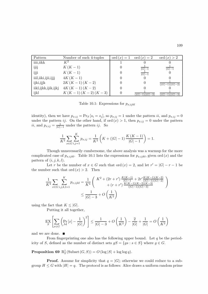
109

Pattern Number of such 4-tuples ord (x) = 1 ord (x) = 2 ord (x) > 2

iiii,iikk K2 1 0 0ijij K (K − 1) 0 1

|G|−11

|G|−1

ijji K (K − 1) 0 1|G|−1 0

iiil,iiki,ijii,ijjj 4K (K − 1) 0 0 0ijki,ijjk 2K (K − 1) (K − 2) 0 0 1

(|G|−1)(|G|−2)

iikl,ijkk,ijik,ijkj 4K (K − 1) (K − 2) 0 0 0ijkl K (K − 1) (K − 2) (K − 3) 0 1

(|G|−1)(|G|−3)1

(|G|−1)(|G|−3)

Table 10.1: Expressions for px,ijkl

identity), then we have px,ij = PrS [si = sj], so px,ij = 1 under the pattern ii, and px,ij = 0under the pattern ij. On the other hand, if ord (x) > 1, then px,ij = 0 under the patternii, and px,ij = 1

|G|−1 under the pattern ij. So

1

K2

∑

x∈G

K∑

i,j=1

px,ij =1

K2

(K + (|G| − 1)

K (K − 1)

|G| − 1

)= 1.

Though unnecessarily cumbersome, the above analysis was a warmup for the morecomplicated case of px,ijkl. Table 10.1 lists the expressions for px,ijkl, given ord (x) and thepattern of (i, j, k, l).

Let r be the number of x ∈ G such that ord (x) = 2, and let r′ = |G| − r − 1 bethe number such that ord (x) > 2. Then

1

K4

∑

x∈G

K∑

i,j,k,l=1

px,ijkl =1

K4

(K2 + (2r + r′) K(K−1)

|G|−1 + 2r′K(K−1)(K−2)(|G|−1)(|G|−2)

+ (r + r′) K(K−1)(K−2)(K−3)(|G|−1)(|G|−3)

)

≤ 1

|G| − 3+O

(1

K2

)

using the fact that K ≤ |G|.Putting it all together,

EXS

[∑

x∈G

(PrM

[x] − 1

|G|

)2]≤ 1

|G| − 3+O

(1

K2

)− 2

|G| +1

|G| = O

(1

K2

)

and we are done.From fingerprinting one also has the following upper bound. Let q be the period-

icity of S, defined as the number of distinct sets gS = gs : s ∈ S where g ∈ G.

Proposition 69 R12 (Subset (G,S)) = O (log |S| + log log q).

Proof. Assume for simplicity that q = |G|; otherwise we could reduce to a sub-group H ≤ G with |H| = q. The protocol is as follows: Alice draws a uniform random prime

110

p from the range[|S|2 log2 |G| , 2 |S|2 log2 |G|

]; she then sends Bob the pair (p, xmod p)

where x is interpreted as an integer. This takes O (log |S| + log log |G|) bits. Bob outputs1 if and only if there exists a z ∈ G such that zy ∈ S and x ≡ z (mod p). To see theprotocol’s correctness, observe that if x 6= z, then there at most log |G| primes p such that

x− z ≡ 0 (mod p), whereas the relevant range contains Ω(

|S|2 log2|G|log(|S| log|G|)

)primes. Therefore,

if xy /∈ S, then by the union bound

Prp

[∃z : zy ∈ S, x ≡ z (mod p)] = O

(|S| log |G| log (|S| log |G|)

|S|2 log2 |G|

)= o (1) .

10.5 Open Problems

Are R12 (f) and Q1

2 (f) polynomially related for every total Boolean function f? Also, canwe exhibit any asymptotic separation between these measures? The best separation I knowof is a factor of 2: for the equality function we have R1

2 (EQ) ≥ (1 − o (1)) log2 n, whereasWinter [243] has shown that Q1

2 (EQ) ≤ (1/2 + o (1)) log2 n using a protocol involving mixedstates.12 This factor-2 savings is tight for equality: a simple counting argument shows thatQ1

2 (EQ) ≥ (1/2 − o (1)) log2 n; and although the usual randomized protocol for equality[194] uses (2 + o (1)) log2 n bits, there exist protocols based on error-correcting codes thatuse only log2 (cn) = log2 n+O (1) bits. All of this holds for any constant error probability0 < ε < 1/2.

Can we lower-bound Q12 (Coset (G)) for groups other than Z2

p (such as Zn2 , or

nonabelian groups)? Also, can we characterize Q12 (Subset (G,S)) for all sets S, closing the

gap between the upper and lower bounds?Is there an oracle relative to which BQP/poly 6= BQP/qpoly?Can we give oracles relative to which NP ∩ coNP and SZK are not contained in

BQP/qpoly? Even more ambitiously, can we prove a direct product theorem for quantumquery complexity that applies to any partial or total function (not just search)?

For all f (partial or total), is R12 (f) = O (

√n) whenever Q1

2 (f) = O (log n)? Inother words, is the separation of Bar-Yossef et al. [43] the best possible?

Can the result D1 (f) = O(mQ1

2 (f) log Q12 (f)

)for partial f be improved to

D1 (f) = O(mQ1

2 (f))? I do not even know how to rule out D1 (f) = O

(m+ Q1

2 (f)).

In the Simultaneous Messages (SM) model, there is no direct communication be-tween Alice and Bob; instead, Alice and Bob both send messages to a third party called thereferee, who then outputs the function value. The complexity measure is the sum of the two

message lengths. Let R||2 (f) and Q

||2 (f) be the randomized and quantum bounded-error

SM complexities of f respectively, and let R||,pub2 (f) be the randomized SM complexity if

Alice and Bob share an arbitrarily long random string. Building on work by Buhrman et

al. [75], Yao [250] showed that Q||2 (f) = O (log n) whenever R

||,pub2 (f) = O (1). He then

12If we restrict ourselves to pure states, then (1 − o (1)) log2 n qubits are needed. Based on that fact, aprevious version of this chapter claimed incorrectly that Q1

2 (EQ) ≥ (1 − o (1)) log2 n.

111

asked about the other direction: for some ε > 0, does R||,pub2 (f) = O

(n1/2−ε) whenever

Q||2 (f) = O (log n), and does R

||2 (f) = O

(n1−ε) whenever Q

||2 (f) = O (log n)? In an earlier

version of this chapter, I showed that R||2 (f) = O

(√n(R

||,pub2 (f) + log n

)), which means

that a positive answer to Yao’s first question would imply a positive answer to the second.Later I learned that Yao independently proved the same result [249]. Here I ask a related

question: can Q||2 (f) ever be exponentially smaller than R

||,pub2 (f)? (Buhrman et al. [75]

showed that Q||2 (f) can be exponentially smaller than R

||2 (f).) Iordanis Kerenidis has

pointed out to me that, based on the hidden matching problem of Bar-Yossef et al. [43]

discussed in Section 10.1, one can define a relation for which Q||2 (f) is exponentially smaller

than R||,pub2 (f). However, as in the case of Q1

2 (f) versus R12 (f), it remains to extend that

result to functions.

112

Chapter 11

Summary of Part I

From my unbiased perspective, quantum lower bounds are some of the deepestresults to have emerged from the study of quantum computing and information. Theseresults tell us that many problems we thought were intractable based on classical intuition,really are intractable according to our best theory of the physical world. On the other hand,the reasons for intractability are much more subtle than in the classical case. In some sense,this has to be true—for otherwise the reasons would apply even to those problems for whichdramatic quantum speedups exist.

We currently have two methods for proving lower bounds on quantum query com-plexity: the polynomial method of Beals et al. [45], and the adversary method of Ambainis[27]. The preceding chapters have illustrated what, borrowing from Wigner [242], we mightcall the “unreasonable effectiveness” of these methods. Both continue to work far outsideof their original design specs—whether by proving classical lower bounds, lower bounds forexponentially small success probabilities (as in the direct product theorem), or polynomiallower bounds for quantities that have “no right” to be polynomials (as in the collision andset comparison problems). Yet the two methods also have complementary limitations. Theadversary method is useless when the relevant probability gaps are small, or when every0-input differs from every 1-input in a constant fraction of locations. Likewise, the polyno-mial method cannot be applied to problems that lack permutation symmetry, at least usingthe techniques we currently know. Thus, perhaps the most important open problem inquantum lower bounds is to develop a new method that overcomes the limitations of boththe polynomial and the adversary methods.1

In keeping with the theme of this thesis, I end Part I by listing some classicalintuitions about computing, that a hypothetical being from Conway’s Game of Life couldsafely carry into the quantum universe.

• The collision problem is not that much easier than unordered search. For despitebeing extremely far from any one-to-one function, a random two-to-one function stilllooks one-to-one unless we do an expensive search for collisions.

• Finding a local minimum of a function is not that much easier than finding a global

1Along these lines, Barnum, Saks, and Szegedy [44] have given what in some sense is a provably optimalmethod, but their method (based on semidefinite programming) seems too difficult to apply directly.

113

minimum. This is because the paths leading to local minima could be exponentiallylong.

• If we want to distinguish an input X from the set of all Y such that f (Y ) 6= f (X),then there is nothing much better to do than to query nonadaptively according to theminimax strategy.

• The difficulty of recursive Fourier sampling increases exponentially with the height ofthe tree.

• Given n unrelated instances of a problem, but only enough time to solve o (n) of them,the probability of succeeding on all n instances decreases exponentially with n.

• NP-complete problems are probably hard, even with the help of polynomial-size ad-vice.

114

Part II

Models and Reality

115

LS: So you believe quantum mechanics?

Me: Of course I do!

LS: So a thousand years from now, people will still be doing quantum mechanics?

Me: Well. . . um. . . I guess so. . .

—Conversation between me and Lee Smolin

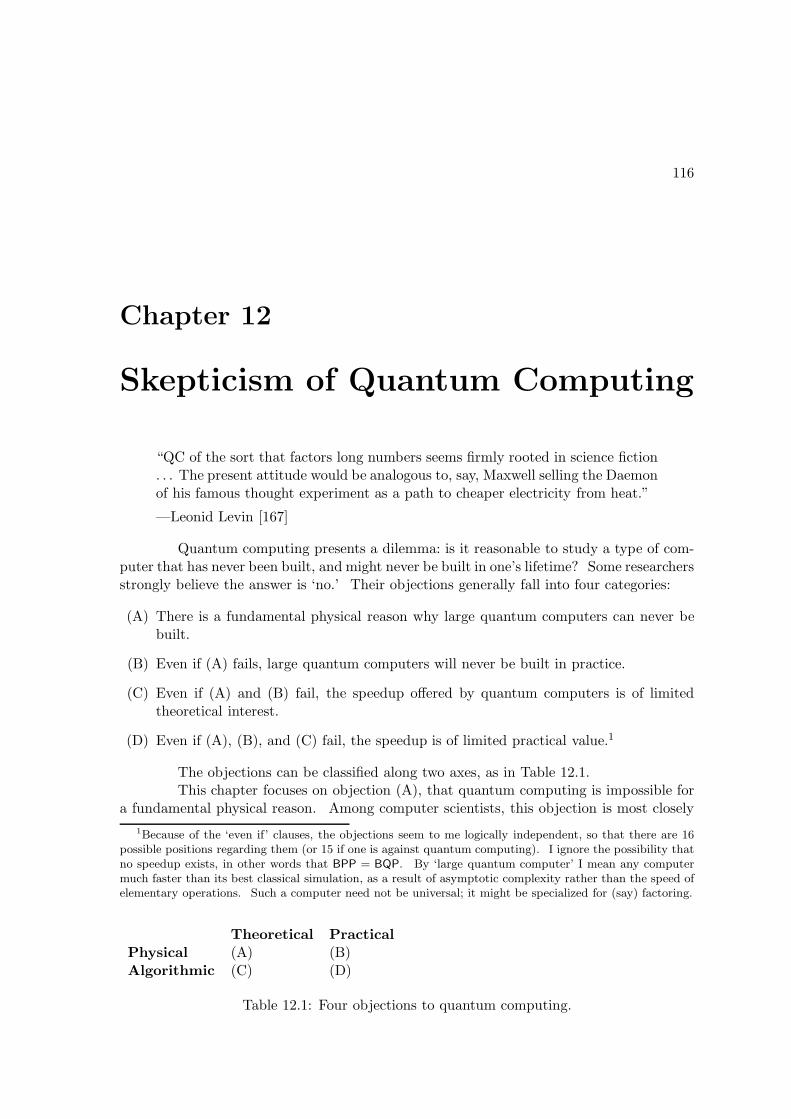
116

Chapter 12

Skepticism of Quantum Computing

“QC of the sort that factors long numbers seems firmly rooted in science fiction. . . The present attitude would be analogous to, say, Maxwell selling the Daemonof his famous thought experiment as a path to cheaper electricity from heat.”

—Leonid Levin [167]

Quantum computing presents a dilemma: is it reasonable to study a type of com-puter that has never been built, and might never be built in one’s lifetime? Some researchersstrongly believe the answer is ‘no.’ Their objections generally fall into four categories:

(A) There is a fundamental physical reason why large quantum computers can never bebuilt.

(B) Even if (A) fails, large quantum computers will never be built in practice.

(C) Even if (A) and (B) fail, the speedup offered by quantum computers is of limitedtheoretical interest.

(D) Even if (A), (B), and (C) fail, the speedup is of limited practical value.1

The objections can be classified along two axes, as in Table 12.1.This chapter focuses on objection (A), that quantum computing is impossible for

a fundamental physical reason. Among computer scientists, this objection is most closely

1Because of the ‘even if’ clauses, the objections seem to me logically independent, so that there are 16possible positions regarding them (or 15 if one is against quantum computing). I ignore the possibility thatno speedup exists, in other words that BPP = BQP. By ‘large quantum computer’ I mean any computermuch faster than its best classical simulation, as a result of asymptotic complexity rather than the speed ofelementary operations. Such a computer need not be universal; it might be specialized for (say) factoring.

Theoretical PracticalPhysical (A) (B)Algorithmic (C) (D)

Table 12.1: Four objections to quantum computing.

117

associated with Leonid Levin [167].2 The following passage captures much of the flavor ofhis critique:

The major problem [with quantum computing] is the requirement that basicquantum equations hold to multi-hundredth if not millionth decimal positionswhere the significant digits of the relevant quantum amplitudes reside. Wehave never seen a physical law valid to over a dozen decimals. Typically, everyfew new decimal places require major rethinking of most basic concepts. Arequantum amplitudes still complex numbers to such accuracies or do they becomequaternions, colored graphs, or sick-humored gremlins? [167]

Among other things, Levin argues that quantum computing is analogous to theunit-cost arithmetic model, and should be rejected for essentially the same reasons; thatclaims to the contrary rest on a confusion between metric and topological approximation;that quantum fault-tolerance theorems depend on extravagant assumptions; and that evenif a quantum computer failed, we could not measure its state to prove a breakdown ofquantum mechanics, and thus would be unlikely to learn anything new.

A few responses to Levin’s arguments can be offered immediately. First, evenclassically, one can flip a coin a thousand times to produce probabilities of order 2−1000.Should one dismiss such probabilities as unphysical? At the very least, it is not obviousthat amplitudes should behave differently than probabilities with respect to error—sinceboth evolve linearly, and neither is directly observable.

Second, if Levin believes that quantum mechanics will fail, but is agnostic aboutwhat will replace it, then his argument can be turned around. How do we know that thesuccessor to quantum mechanics will limit us to BPP, rather than letting us solve (say)PSPACE-complete problems? This is more than a logical point. Abrams and Lloyd [15]argue that a wide class of nonlinear variants of the Schrodinger equation would allow NP-complete and even #P-complete problems to be solved in polynomial time. And Penrose[191], who proposed a model for ‘objective collapse’ of the wavefunction, believes that hisproposal takes us outside the set of computable functions entirely!

Third, to falsify quantum mechanics, it would suffice to show that a quantumcomputer evolved to some state far from the state that quantum mechanics predicts. Mea-suring the exact state is unnecessary. Nobel prizes have been awarded in the past ‘merely’for falsifying a previously held theory, rather than replacing it by a new one. An exampleis the physics Nobel awarded to Fitch [112] and Cronin [89] in 1980 for discovering CPsymmetry violation.

Perhaps the key to understanding Levin’s unease about quantum computing liesin his remark that “we have never seen a physical law valid to over a dozen decimals.” Herehe touches on a serious epistemological question: How far should we extrapolate from today’sexperiments to where quantum mechanics has never been tested? I will try to address thisquestion by reviewing the evidence for quantum mechanics. For my purposes it will not

2More recently, Oded Goldreich [130] has also put forward an argument against quantum computing.Compared to Levin’s arguments, Goldreich’s is easily understood: he believes that states arising in Shor’salgorithm have exponential “non-degeneracy” and therefore take exponential time to prepare, and that thereis no burden on those who hold this view to suggest a definition of non-degeneracy.

118

suffice to declare the predictions of quantum mechanics “verified to one part in a trillion,”because we have to distinguish at least three different types of prediction: interference,entanglement, and Schrodinger cats. Let us consider these in turn.

(1) Interference. If the different paths that an electron could take in its orbit around anucleus did not interfere destructively, canceling each other out, then electrons wouldnot have quantized energy levels. So being accelerating electric charges, they wouldlose energy and spiral into their respective nuclei, and all matter would disintegrate.That this has not happened—together with the results of (for example) single-photondouble-slit experiments—is compelling evidence for the reality of quantum interfer-ence.

(2) Entanglement. One might accept that a single particle’s position is described by awave in three-dimensional phase space, but deny that two particles are described bya wave in six -dimensional phase space. However, the Bell inequality experiments ofAspect et al. [37] and successors have convinced all but a few physicists that quantumentanglement exists, can be maintained over large distances, and cannot be explainedby local hidden-variable theories.

(3) Schrodinger Cats. Accepting two- and three-particle entanglement is not the sameas accepting that whole molecules, cats, humans, and galaxies can be in coherentsuperposition states. However, recently Arndt et al. [35] have performed the double-slit interference experiment using C60 molecules (buckyballs) instead of photons; whileFriedman et al. [121] have found evidence that a superconducting current, consisting ofbillions of electrons, can enter a coherent superposition of flowing clockwise around acoil and flowing counterclockwise (see Leggett [166] for a survey of such experiments).Though short of cats, these experiments at least allow us to say the following: ifwe could build a general-purpose quantum computer with as many components ashave already been placed into coherent superposition, then on certain problems, thatcomputer would outperform any computer in the world today.

Having reviewed some of the evidence for quantum mechanics, we must now askwhat alternatives have been proposed that might also explain the evidence. The simplestalternatives are those in which quantum states “spontaneously collapse” with some proba-bility, as in the GRW (Ghirardi-Rimini-Weber) theory [125].3 The drawbacks of the GRWtheory include violations of energy conservation, and parameters that must be fine-tunedto avoid conflicting with experiments. More relevant for us, though, is that the collapsespostulated by the theory are only in the position basis, so that quantum information storedin internal degrees of freedom (such as spin) is unaffected. Furthermore, even if we ex-tended the theory to collapse those internal degrees, large quantum computers could stillbe built. For the theory predicts roughly one collapse per particle per 1015 seconds, with acollapse affecting everything in a 10−7-meter vicinity. So even in such a vicinity, one couldperform a computation involving (say) 1010 particles for 105 seconds. Finally, as pointed

3Penrose [191] has proposed another such theory, but as mentioned earlier, his theory suggests that thequantum computing model is too restrictive.

119

out to me by Rob Spekkens, standard quantum error-correction techniques might be usedto overcome even GRW-type decoherence.

A second class of alternatives includes those of ’t Hooft [229] and Wolfram [246],in which something like a deterministic cellular automaton underlies quantum mechanics.On the basis of his theory, ’t Hooft predicts that “[i]t will never be possible to construct a‘quantum computer’ that can factor a large number faster, and within a smaller region ofspace, than a classical machine would do, if the latter could be built out of parts at leastas large and as slow as the Planckian dimensions” [229]. Similarly, Wolfram states that“[i]ndeed within the usual formalism [of quantum mechanics] one can construct quantumcomputers that may be able to solve at least a few specific problems exponentially fasterthan ordinary Turing machines. But particularly after my discoveries . . . I strongly suspectthat even if this is formally the case, it will still not turn out to be a true representation ofultimate physical reality, but will instead just be found to reflect various idealizations madein the models used so far” [246, p.771].

The obvious question then is how these theories account for Bell inequality viola-tions. I confess to being unable to understand ’t Hooft’s answer to this question, exceptthat he believes that the usual notions of causality and locality might no longer apply inquantum gravity. As for Wolfram’s theory, which involves “long-range threads” to accountfor Bell inequality violations, I will show in Section 12.1 below that it fails Wolfram’s owndesiderata of causal and relativistic invariance.

12.1 Bell Inequalities and Long-Range Threads

This section is excerpted from my review [1] of Stephen Wolfram’s A New Kindof Science [246].

The most interesting chapter of A New Kind of Science is the ninth, on ‘Fun-damental Physics.’ Here Wolfram confronts general relativity and quantum mechanics,arguably the two most serious challenges to the deterministic, cellular-automaton-basedview of nature that he espouses. Wolfram conjectures that spacetime is discrete at thePlanck scale, of about 10−33 centimeters or 10−43 seconds. This conjecture is not new, andhas received considerable attention recently in connection with the holographic principle[65] from black hole thermodynamics, which Wolfram does not discuss. But are new ideasoffered to substantiate the conjecture?

For Wolfram, spacetime is a causal network, in which events are vertices and edgesspecify the dependence relations between events. Pages 486–496 and 508–515 discuss indetail how to generate such a network from a simple set of rules. In particular, we couldstart with a finite undirected ‘space graph’ G. We then posit a set of update rules, each ofwhich replaces a subgraph by another subgraph with the same number of outgoing edges.The new subgraph must preserve any symmetries of the old one. Then each event inthe causal network corresponds to an application of an update rule. If updating event Bbecomes possible as a result of event A, then we draw an edge from A to B.

Properties of space are defined in terms of G. For example, if the number ofvertices in G at distance at most n from any given vertex grows as nD, then space can be

120

said to have dimension D. (As for formalizing this definition, Wolfram says only that thereare “some subtleties. For example, to find a definite volume growth rate one does still needto take some kind of limit—and one needs to avoid sampling too many or too few” vertices(p. 1030).) Similarly, Wolfram argues that the curvature information needed for generalrelativity, in particular the Ricci tensor, can be read from the connectivity pattern of G.Interestingly, to make the model as simple as possible, Wolfram does not associate a bit toeach vertex of G, representing (say) the presence or absence of a particle. Instead particlesare localized structures, or ‘tangles,’ in G.

An immediate problem is that one might obtain many nonequivalent causal net-works, depending on the order in which update rules are applied to G. Wolfram calls a setof rules that allows such nondeterministic evolution a ‘multiway system.’ He recognizes,but rejects, a possible connection to quantum mechanics:

The notion of ‘many-figured time’ has been discussed since the 1950s in the con-text of the many-worlds interpretation of quantum mechanics. There are somesimilarities to the multiway systems that I consider here. But an importantdifference is that while in the many-worlds approach, branchings are associatedwith possible observation or measurement events, what I suggest here is thatthey could be an intrinsic feature of even the very lowest-level rules for theuniverse (p. 1035-6).

It is unclear exactly what distinction is being drawn: is there any physical eventthat is not associated with a possible observation or measurement? In any case, Wolframopts instead for rule sets that are ‘causal invariant’: that is, that yield the same causalnetwork regardless of the order in which rules are applied. As noted by Wolfram, asufficient (though not necessary) condition for causal invariance is that no ‘replaceable’subgraph overlaps itself or any other replaceable subgraph.

Wolfram points out an immediate analogy to special relativity, wherein observersdo not in general agree on the order in which spacelike separated events occur, yet agreeon any final outcome of the events. He is vague, though, about how (say) the Lorentztransformations might be derived in a causal network model:

There are many subtleties here, and indeed to explain the details of what isgoing on will no doubt require quite a few new and rather abstract concepts.But the general picture that I believe will emerge is that when particles movefaster they will appear to have more nodes associated with them (p. 529).

Wolfram is “certainly aware that many physicists will want to know more details,”he says in the endnotes, about how a discrete model of the sort he proposes can reproduceknown features of physics. But, although he chose to omit technical formalism from thepresentation, “[g]iven my own personal background in theoretical physics it will come as nosurprise that I have often used such formalism in the process of working out what I describein these sections” (p. 1043). The paradox is obvious: if technical formalism would helpconvince physicists of his ideas, then what could Wolfram lose by including it, say in theendnotes? If, on the other hand, such formalism is irrelevant, then why does Wolfram evenmention having used it?

121

Physicists’ hunger for details will likely grow further when they read the section on‘Quantum Phenomena’ (p. 537–545). Here Wolfram maintains that quantum mechanicsis only an approximation to an underlying classical (and most likely deterministic) theory.Many physicists have sought such a theory, from Einstein to (in modern times) ’t Hooft[229]. But a series of results, beginning in the 1960’s, has made it clear that such a theorycomes at a price. I will argue that, although Wolfram discusses these results, he has notunderstood what they actually entail.

To begin, Wolfram is not advocating a hidden-variable approach such as Bohmianmechanics, in which the state vector is supplemented by an ‘actual’ eigenstate of a particularobservable. Instead he thinks that, at the lowest level, the state vector is not needed at all;it is merely a useful construct for describing some (though presumably not all) higher-levelphenomena. Indeterminacy arises because of one’s inability to know the exact state of asystem:

[I]f one knew all of the underlying details of the network that makes up ouruniverse, it should always be possible to work out the result of any measurement.I strongly believe that the initial conditions for the universe were quite simple.But like many of the processes we have seen in this book, the evolution of theuniverse no doubt intrinsically generates apparent randomness. And the resultis that most aspects of the network that represents the current state of ouruniverse will seem essentially random (p. 543).

Similarly, Wolfram explains as follows why an electron has wave properties: “. . . anetwork which represents our whole universe must also include us as observers. And thismeans that there is no way that we can look at the network from the outside and see theelectron as a definite object” (p. 538). An obvious question then is how Wolfram accountsfor the possibility of quantum computing, assuming BPP 6= BQP. He gives an answer inthe final chapter:

Indeed within the usual formalism [of quantum mechanics] one can constructquantum computers that may be able to solve at least a few specific problemsexponentially faster than ordinary Turing machines. But particularly after mydiscoveries in Chapter 9 [‘Fundamental Physics’], I strongly suspect that evenif this is formally the case, it will still not turn out to be a true representationof ultimate physical reality, but will instead just be found to reflect variousidealizations made in the models used so far (p. 771).

In the endnotes, though, where he explains quantum computing in more detail,Wolfram seems to hedge about which idealizations he has in mind:

It does appear that only modest precision is needed for the initial amplitudes.And it seems that perturbations from the environment can be overcome usingversions of error-correcting codes. But it remains unclear just what might beneeded actually to perform for example the final measurements required (p.1148).

122

One might respond that, with or without quantum computing, Wolfram’s propos-als can be ruled out on the simpler ground that they disallow Bell inequality violations.However, Wolfram puts forward an imaginative hypothesis to account for bipartite entan-glement. When two particles (or ‘tangles’ in the graph G) collide, long-range ‘threads’ mayform between them, which remain in place even if the particles are later separated:

The picture that emerges is then of a background containing a very large num-ber of connections that maintain an approximation to three-dimensional space,together with a few threads that in effect go outside of that space to make directconnections between particles (p. 544).

The threads can produce Bell correlations, but are somehow too small (i.e. containtoo few edges) to transmit information in a way that violates causality.

There are several objections one could raise against this thread hypothesis. WhatI will show is that, if one accepts two of Wolfram’s own desiderata—determinism and causalinvariance—then the hypothesis fails. First, though, let me remark that Wolfram says littleabout what, to me, is a more natural possibility than the thread hypothesis. This is anexplicitly quantum cellular automaton or causal network, with a unitary transition rule.The reason seems to be that he does not want continuity anywhere in a model, not evenin probabilities or amplitudes. In the notes, he describes an experiment with a quantumcellular automaton as follows:

One might hope to be able to get an ordinary cellular automaton with a limitedset of possible values by choosing a suitable [phase rotation] θ [θ = π/4 andθ = π/3 are given as examples in an illustration]. But in fact in non-trivialcases most of the cells generated at each step end up having distinct values (p.1060).

This observation is unsurprising, given the quantum computing results mentionedin Chapter 4, to the effect that almost any nontrivial gate set is universal (that is, canapproximate any unitary matrix to any desired precision, or any orthogonal matrix in caseone is limited to reals). Indeed, Shi [219] has shown that a Toffoli gate, plus any gate thatdoes not preserve the computational basis, or a controlled-NOT gate plus any gate whosesquare does not preserve the computational basis, are both universal gate sets. In anycase, Wolfram does not address the fact that continuity in amplitudes seems more ‘benign’than continuity in measurable quantities: the former, unlike the latter, does not enable aninfinite amount of computation to be performed in a finite time. Also, as observed byBernstein and Vazirani [55], the linearity of quantum mechanics implies that tiny errors inamplitudes will not be magnified during a quantum computation.

I now proceed to the argument that Wolfram’s thread hypothesis is inconsistentwith causal invariance and relativity. Let R be a set of graph updating rules, whichmight be probabilistic. Then consider the following four assertions (which, though notmathematically precise, will be clarified by subsequent discussion).

(1) R satisfies causal invariance. That is, given any initial graph (and choice of random-ness if R is probabilistic), R yields a unique causal network.

123

(2) R satisfies the relativity postulate. That is, assuming the causal network approx-imates a flat Minkowski spacetime at a large enough scale, there are no preferredinertial frames.

(3) R permits Bell inequality violations.

(4) Any updating rule in R is always considered to act on a fixed graph, not on a distri-bution or superposition over graphs. This is true even if parts of the initial graphare chosen at random, and even if R is probabilistic.

The goal is to show that, for any R, at least one of these assertions is false. Currentphysical theory would suggest that (1)-(3) are true and that (4) is false. Wolfram, if Iunderstand him correctly, starts with (4) as a premise, and then introduces causal invarianceto satisfy (1) and (2), and long-range threads to satisfy (3). Of course, even to state thetwo-party Bell inequalities requires some notion of randomness. And on pages 299–326,Wolfram discusses three mechanisms for introducing randomness into a system: randomnessin initial conditions, randomness from the environment (i.e. probabilistic updating rules),and intrinsic randomness (i.e. deterministic rules that produce pseudorandom output).However, all of these mechanisms are compatible with (4), and so my argument will showthat they are inadequate assuming (1)-(3). The conclusion is that, in a model of the sortWolfram considers, randomness must play a more fundamental role than he allows.

In a standard Bell experiment, Alice and Bob are given input bits xA and xBrespectively, chosen uniformly and independently at random. Their goal is, without com-municating, to output bits yA and yB respectively such that yA ⊕ yB = xA ∧ xB . Underany ‘local hidden variable’ theory, Alice and Bob can succeed with probability at most 3/4;the optimal strategy is for them to ignore their inputs and output (say) yA = 0 and yB = 0.However, suppose Alice has a qubit ρA and Bob a ρB, that are jointly in the Bell state(|00〉 + |11〉) /

√2. Then there is a protocol4 by which they can succeed with probability(

5 +√

2)/8 ≈ 0.802.To model this situation, let A and B, corresponding to Alice and Bob, be disjoint

subgraphs of a graph G. Suppose that, at a large scale, G approximates a Euclideanspace of some dimension; and that any causal network obtained by applying updates toG approximates a Minkowski spacetime. One can think of G as containing long-rangethreads from A to B, though the nature of the threads will not affect the conclusions.Encode Alice’s input xA by (say) placing an edge between two specific vertices in A if andonly if xA = 1. Encode xB similarly, and also supply Alice and Bob with arbitrarilymany correlated random bits. Finally, let us stipulate that at the end of the protocol,there is an edge between two specific vertices in A if and only if yA = 1, and similarly foryB. A technicality is that we need to be able to identify which vertices correspond to xA,yA, and so on, even as G evolves over time. We could do this by stipulating that (say)“the xA vertices are the ones that are roots of complete binary trees of depth 3,” and thenchoosing the rule set to guarantee that, throughout the protocol, exactly two vertices havethis property.

4If xA = 1 then Alice applies a π/8 phase rotation to ρA, and if xB = 1 then Bob applies a −π/8 rotationto ρB. Both parties then measure in the standard basis and output whatever they observe.

124

Call a variable ‘touched’ after an update has been applied to a subgraph containingany of the variable’s vertices. Also, let Z be an assignment to all random variables: thatis, xA, xB , the correlated random bits, and the choice of randomness if R is probabilistic.Then for all Z we need the following, based on what observers in different inertial framescould perceive:

(i) There exists a sequence of updates under which yA is output before any of Bob’svariables are touched.

(ii) There exists another sequence under which yB is output before any of Alice’s variablesare touched.

Now it is easy to see that, if a Bell inequality violation occurs, then causal invari-

ance must be violated. Given Z, let y(1)A (Z), y

(1)B (Z) be the values of yA, yB that are output

under rule sequence (i), and let y(2)A (Z), y

(2)B (Z) be the values output under sequence (ii).

Then there must exist some Z for which either y(1)A (Z) 6= y

(2)A (Z) or y

(1)B (Z) 6= y

(2)B (Z)—for

if not, then the entire protocol could be simulated under a local hidden variable model. Itfollows that the outcome of the protocol can depend on the order in which updates areapplied.

To obtain a Bell inequality violation, something like the following seems to beneeded. We can encode ‘hidden variables’ into G, representing the outcomes of the possiblemeasurements Bob could make on ρB . (We can imagine, if we like, that the update rulesare such that observing any one of these variables destroys all the others. Also, we make noassumption of contextuality.) Then, after Alice measures ρA, using the long-range threadsshe updates Bob’s hidden variables conditioned on her measurement outcome. Similarly,Bob updates Alice’s hidden variables conditioned on his outcome. Since at least one partymust access its hidden variables for there to be Bell inequality violations, causal invarianceis still violated. But a sort of probabilistic causal invariance holds, in the sense that ifwe marginalize out A (the ‘Alice’ part of G), then the distribution of values for each ofBob’s hidden variables is the same before and after Alice’s update. The lesson is that, ifwe want both causal invariance and Bell inequality violations, then we need to introduceprobabilities at a fundamental level—not merely to represent Alice and Bob’s subjectiveuncertainty about the state of G, but even to define whether a set of rules is or is not causalinvariant.

Note that I made no assumption about how the random bits were generated—i.e.whether they were ‘truly random’ or were the pseudorandom output of some updating rule.The conclusion is also unaffected if we consider a ‘deterministic’ variant of Bell’s theorem dueto Greenberger, Horne, and Zeilinger [138]. There three parties, Alice, Bob, and Charlie, aregiven input bits xA, xB, and xC respectively, satisfying the promise that xA⊕xB⊕xC = 0.The goal is to output bits yA, yB, and yC such that yA ⊕ yB ⊕ yC = xA ∨ xB ∨ xC .Under a local hidden variable model, there is no protocol that succeeds on all four possibleinputs; but if the parties share the GHZ state (|011〉 + |101〉 + |110〉 − |000〉) /2, then sucha protocol exists. However, although the output is correct with certainty, assuming causalinvariance one cannot implement the protocol without introducing randomness into theunderlying rules, exactly as in the two-party case.

125

After a version of the above argument was sent to Wolfram, Todd Rowland, anemployee of Wolfram, sent me email claiming that the argument fails for the followingreason. I assumed that there exist two sequences of updating events, one in which Alice’smeasurement precedes Bob’s and one in which Bob’s precedes Alice’s. But I neglectedthe possibility that a single update, call it E, is applied to a subgraph that straddles thelong-range threads. The event E would encompass both Alice and Bob’s measurements, sothat neither would precede the other in any sequence of updates. We could thereby obtaina rule set R satisfying assertions (1), (3), and (4).

I argue that such an R would nevertheless fail to satisfy (2). For in effect we startwith a flat Minkowski spacetime, and then take two distinct events that are simultaneousin a particular inertial frame, and identify them as being the same event E. This can bevisualized as ‘pinching together’ two horizontally separated points on a spacetime diagram.(Actually a whole ‘V’ of points must be pinched together, since otherwise entanglementcould not have been created.) However, what happens in a different inertial frame? Itwould seem that E, a single event, is perceived to occur at two separate times. That byitself might be thought acceptable, but it implies that there exists a class of preferred inertialframes: those in which E is perceived to occur only once. Of course, even in a flat spacetime,one could designate as ‘preferred’ those frames in which Alice and Bob’s measurements areperceived to be simultaneous. A crucial distinction, though, is that there one only obtainsa class of preferred frames after deciding which event at Alice’s location, and which at Bob’slocation, should count as the ‘measurement.’ Under Rowland’s hypothesis, by contrast,once one decides what counts as the measurement at Alice’s location, the decision at Bob’slocation is made automatically, because of the identification of events that would otherwisebe far apart.

126

Chapter 13

Complexity Theory of QuantumStates

In my view, the central weakness in the arguments of quantum computing skepticsis their failure to suggest any answer the following question: Exactly what property separatesthe quantum states we are sure we can create, from the states that suffice for Shor’s factoringalgorithm?

I call such a property a “Sure/Shor separator.” The purpose of this chapter isto develop a mathematical theory of Sure/Shor separators, and thereby illustrate what Ithink a scientific discussion about the possibility of quantum computing might look like.In particular, I will introduce tree states, which informally are those states |ψ〉 ∈ H⊗n

2

expressible by a polynomial-size ‘tree’ of addition and tensor product gates. For example,α |0〉⊗n + β |1〉⊗n and (α |0〉 + β |1〉)⊗n are both tree states. Section 13.1 provides thephilosophical motivation for thinking of tree states as a possible Sure/Shor separator; thenSection 13.2 formally defines tree states and many related classes of quantum states. Next,Section 13.3 investigates basic properties of tree states. Among other results, it showsthat any tree state is representable by a tree of polynomial size and logarithmic depth; andthat most states do not even have large inner product with any tree state. Then Section13.4 shows relationships among tree size, circuit size, bounded-depth tree size, Vidal’s χcomplexity [236], and several other measures. It also relates questions about quantum stateclasses to more traditional questions about computational complexity classes.

But the main results of the chapter, proved in Section 13.5, are lower boundson tree size for various natural families of quantum states. In particular, Section 13.5.1analyzes “subgroup states,” which are uniform superpositions |S〉 over all elements of asubgroup S ≤ Zn2 . The importance of these states arises from their central role in sta-bilizer codes, a type of quantum error-correcting code. I first show that if S is chosenuniformly at random, then with high probability |S〉 cannot be represented by any tree ofsize no(logn). This result has a corollary of independent complexity-theoretic interest: thefirst superpolynomial gap between the formula size and the multilinear formula size of afunction f : 0, 1n → R. I then present two improvements of the basic lower bound. First,I show that a random subgroup state cannot even be approximated well in trace distance byany tree of size no(logn). Second, I “derandomize” the lower bound, by using Reed-Solomon

127

codes to construct an explicit subgroup state with tree size nΩ(logn).Section 13.5.2 analyzes the states that arise in Shor’s factoring algorithm—for

example, a uniform superposition over all multiples of a fixed positive integer p, written inbinary. Originally, I had hoped to show a superpolynomial tree size lower bound for thesestates as well. However, I am only able to show such a bound assuming a number-theoreticconjecture.

The lower bounds use a sophisticated recent technique of Raz [197, 198], which wasintroduced to show that the permanent and determinant of a matrix require superpolynomial-size multilinear formulas. Currently, Raz’s technique is only able to show lower bounds ofthe form nΩ(logn), but I conjecture that 2Ω(n) lower bounds hold in all of the cases discussedabove.

One might wonder how superpolynomial tree size relates to more physical proper-ties of a quantum state. Section 13.5.3 addresses this question, by pointing out how Raz’slower bound technique is connected to a notion that physicists call “persistence of entan-glement” [71, 102]. On the other hand, I also give examples showing that the connectionis not exact.

Section 13.6 studies a weakening of tree size called “manifestly orthogonal treesize,” and shows that this measure can sometimes be characterized exactly, enabling us toprove exponential lower bounds. The techniques in Section 13.6 might be of independentinterest to complexity theorists—one reason being that they do not obviously “naturalize”in the sense of Razborov and Rudich [202].

Section 13.7 addresses the following question. If the state of a quantum computerat every time step is a tree state, then can the computer be simulated classically? Inother words, letting TreeBQP be the class of languages accepted by such a machine, doesTreeBQP = BPP? A positive answer would make tree states more attractive as a Sure/Shorseparator. For once we admit any states incompatible with the polynomial-time Church-Turing thesis, it seems like we might as well go all the way, and admit all states preparableby polynomial-size quantum circuits! Although I leave this question open, I do show thatTreeBQP ⊆ ΣP

3 ∩ΠP3 , where ΣP

3 ∩ΠP3 is the third level of the polynomial hierarchy PH. By

contrast, it is conjectured that BQP 6⊂ PH, though admittedly not on strong evidence.Section 13.8 discusses the implications of these results for experimental physics.

It advocates a dialogue between theory and experiment, in which theorists would proposea class of quantum states that encompasses everything seen so far, and then experimenterswould try to prepare states not in that class. It also asks whether states with superpolyno-mial tree size have already been observed in condensed-matter systems; and more broadly,what sort of evidence is needed to establish a state’s existence. Other issues addressed inSection 13.8 include how to deal with mixed states and particle position and momentumstates, and the experimental relevance of asymptotic bounds. I conclude in Section 13.9with some open problems.

13.1 Sure/Shor Separators

Given the discussion in Chapter 12, I believe that the challenge for quantum computingskeptics is clear. Ideally, come up with an alternative to quantum mechanics—even an

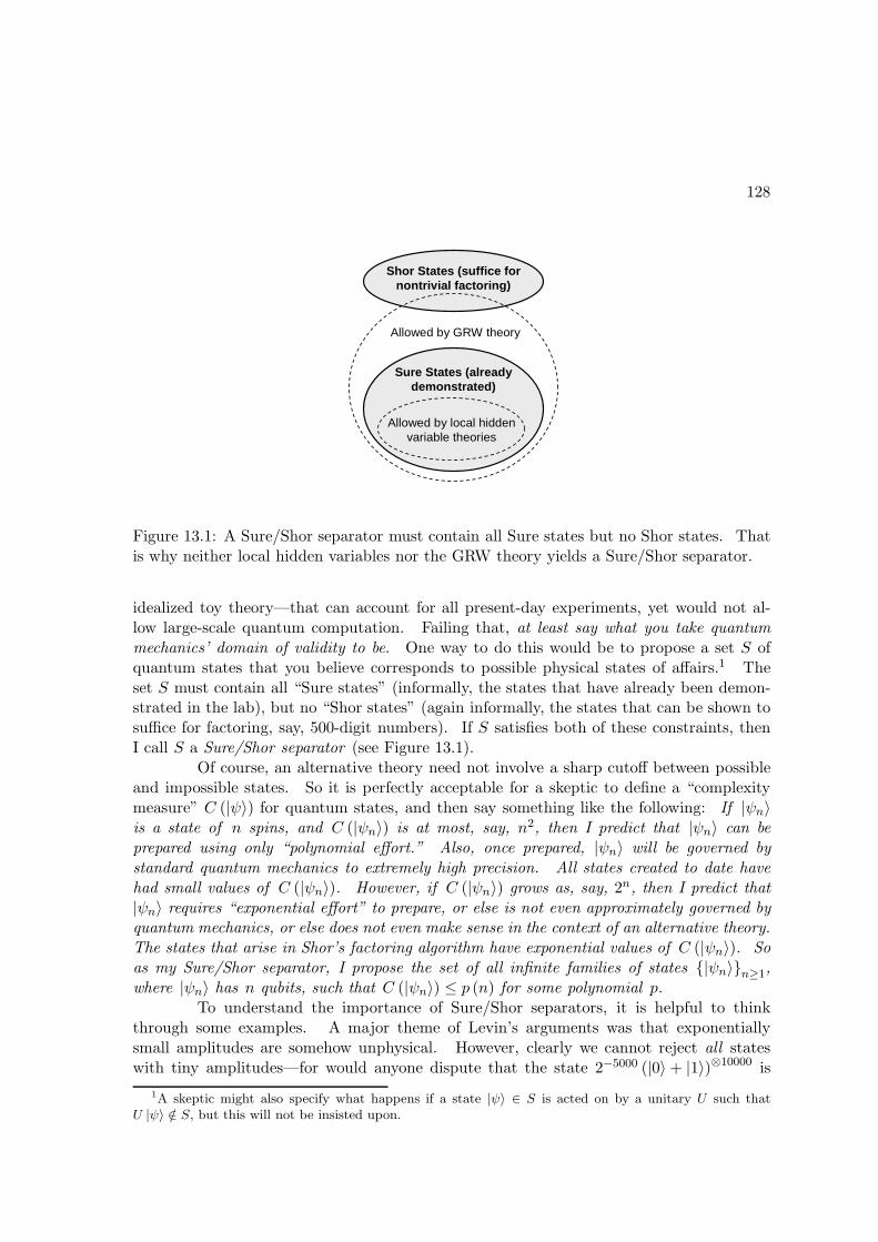
128

Sure States (already demonstrated)

Shor States (suffice for nontrivial factoring)

Allowed by local hidden variable theories

Allowed by GRW theory

Figure 13.1: A Sure/Shor separator must contain all Sure states but no Shor states. Thatis why neither local hidden variables nor the GRW theory yields a Sure/Shor separator.

idealized toy theory—that can account for all present-day experiments, yet would not al-low large-scale quantum computation. Failing that, at least say what you take quantummechanics’ domain of validity to be. One way to do this would be to propose a set S ofquantum states that you believe corresponds to possible physical states of affairs.1 Theset S must contain all “Sure states” (informally, the states that have already been demon-strated in the lab), but no “Shor states” (again informally, the states that can be shown tosuffice for factoring, say, 500-digit numbers). If S satisfies both of these constraints, thenI call S a Sure/Shor separator (see Figure 13.1).

Of course, an alternative theory need not involve a sharp cutoff between possibleand impossible states. So it is perfectly acceptable for a skeptic to define a “complexitymeasure” C (|ψ〉) for quantum states, and then say something like the following: If |ψn〉is a state of n spins, and C (|ψn〉) is at most, say, n2, then I predict that |ψn〉 can beprepared using only “polynomial effort.” Also, once prepared, |ψn〉 will be governed bystandard quantum mechanics to extremely high precision. All states created to date havehad small values of C (|ψn〉). However, if C (|ψn〉) grows as, say, 2n, then I predict that|ψn〉 requires “exponential effort” to prepare, or else is not even approximately governed byquantum mechanics, or else does not even make sense in the context of an alternative theory.The states that arise in Shor’s factoring algorithm have exponential values of C (|ψn〉). Soas my Sure/Shor separator, I propose the set of all infinite families of states |ψn〉n≥1,where |ψn〉 has n qubits, such that C (|ψn〉) ≤ p (n) for some polynomial p.

To understand the importance of Sure/Shor separators, it is helpful to thinkthrough some examples. A major theme of Levin’s arguments was that exponentiallysmall amplitudes are somehow unphysical. However, clearly we cannot reject all stateswith tiny amplitudes—for would anyone dispute that the state 2−5000 (|0〉 + |1〉)⊗10000 is

1A skeptic might also specify what happens if a state |ψ〉 ∈ S is acted on by a unitary U such thatU |ψ〉 /∈ S, but this will not be insisted upon.

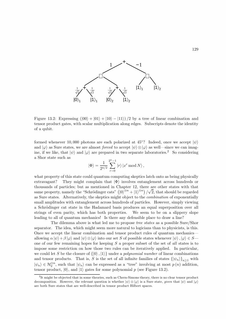
129

+

⊗

|1⟩1 |1⟩2

⊗

++

|0⟩1 |1⟩1 |0⟩2 |1⟩2

1

2

1

2

1

2

1

2

1−1

Figure 13.2: Expressing (|00〉 + |01〉 + |10〉 − |11〉) /2 by a tree of linear combination andtensor product gates, with scalar multiplication along edges. Subscripts denote the identityof a qubit.

formed whenever 10, 000 photons are each polarized at 45? Indeed, once we accept |ψ〉and |ϕ〉 as Sure states, we are almost forced to accept |ψ〉⊗ |ϕ〉 as well—since we can imag-ine, if we like, that |ψ〉 and |ϕ〉 are prepared in two separate laboratories.2 So consideringa Shor state such as

|Φ〉 =1

2n/2

2n−1∑

r=0

|r〉 |xr modN〉 ,

what property of this state could quantum computing skeptics latch onto as being physicallyextravagant? They might complain that |Φ〉 involves entanglement across hundreds orthousands of particles; but as mentioned in Chapter 12, there are other states with thatsame property, namely the “Schrodinger cats”

(|0〉⊗n + |1〉⊗n

)/√

2, that should be regardedas Sure states. Alternatively, the skeptics might object to the combination of exponentiallysmall amplitudes with entanglement across hundreds of particles. However, simply viewinga Schrodinger cat state in the Hadamard basis produces an equal superposition over allstrings of even parity, which has both properties. We seem to be on a slippery slopeleading to all of quantum mechanics! Is there any defensible place to draw a line?

The dilemma above is what led me to propose tree states as a possible Sure/Shorseparator. The idea, which might seem more natural to logicians than to physicists, is this.Once we accept the linear combination and tensor product rules of quantum mechanics—allowing α |ψ〉+β |ϕ〉 and |ψ〉⊗|ϕ〉 into our set S of possible states whenever |ψ〉 , |ϕ〉 ∈ S—one of our few remaining hopes for keeping S a proper subset of the set of all states is toimpose some restriction on how those two rules can be iteratively applied. In particular,we could let S be the closure of |0〉 , |1〉 under a polynomial number of linear combinationsand tensor products. That is, S is the set of all infinite families of states |ψn〉n≥1 with

|ψn〉 ∈ H⊗n2 , such that |ψn〉 can be expressed as a “tree” involving at most p (n) addition,

tensor product, |0〉, and |1〉 gates for some polynomial p (see Figure 13.2).

2It might be objected that in some theories, such as Chern-Simons theory, there is no clear tensor productdecomposition. However, the relevant question is whether |ψ〉 ⊗ |ϕ〉 is a Sure state, given that |ψ〉 and |ϕ〉are both Sure states that are well-described in tensor product Hilbert spaces.

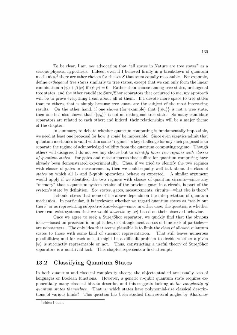
130

To be clear, I am not advocating that “all states in Nature are tree states” as aserious physical hypothesis. Indeed, even if I believed firmly in a breakdown of quantummechanics,3 there are other choices for the set S that seem equally reasonable. For example,define orthogonal tree states similarly to tree states, except that we can only form the linearcombination α |ψ〉 + β |ϕ〉 if 〈ψ|ϕ〉 = 0. Rather than choose among tree states, orthogonaltree states, and the other candidate Sure/Shor separators that occurred to me, my approachwill be to prove everything I can about all of them. If I devote more space to tree statesthan to others, that is simply because tree states are the subject of the most interestingresults. On the other hand, if one shows (for example) that |ψn〉 is not a tree state,then one has also shown that |ψn〉 is not an orthogonal tree state. So many candidateseparators are related to each other; and indeed, their relationships will be a major themeof the chapter.

In summary, to debate whether quantum computing is fundamentally impossible,we need at least one proposal for how it could be impossible. Since even skeptics admit thatquantum mechanics is valid within some “regime,” a key challenge for any such proposal is toseparate the regime of acknowledged validity from the quantum computing regime. Thoughothers will disagree, I do not see any choice but to identify those two regimes with classesof quantum states. For gates and measurements that suffice for quantum computing havealready been demonstrated experimentally. Thus, if we tried to identify the two regimeswith classes of gates or measurements, then we could equally well talk about the class ofstates on which all 1- and 2-qubit operations behave as expected. A similar argumentwould apply if we identified the two regimes with classes of quantum circuits—since any“memory” that a quantum system retains of the previous gates in a circuit, is part of thesystem’s state by definition. So: states, gates, measurements, circuits—what else is there?

I should stress that none of the above depends on the interpretation of quantummechanics. In particular, it is irrelevant whether we regard quantum states as “really outthere” or as representing subjective knowledge—since in either case, the question is whetherthere can exist systems that we would describe by |ψ〉 based on their observed behavior.

Once we agree to seek a Sure/Shor separator, we quickly find that the obviousideas—based on precision in amplitudes, or entanglement across of hundreds of particles—are nonstarters. The only idea that seems plausible is to limit the class of allowed quantumstates to those with some kind of succinct representation. That still leaves numerouspossibilities; and for each one, it might be a difficult problem to decide whether a given|ψ〉 is succinctly representable or not. Thus, constructing a useful theory of Sure/Shorseparators is a nontrivial task. This chapter represents a first attempt.

13.2 Classifying Quantum States

In both quantum and classical complexity theory, the objects studied are usually sets oflanguages or Boolean functions. However, a generic n-qubit quantum state requires ex-ponentially many classical bits to describe, and this suggests looking at the complexity ofquantum states themselves. That is, which states have polynomial-size classical descrip-tions of various kinds? This question has been studied from several angles by Aharonov

3which I don’t

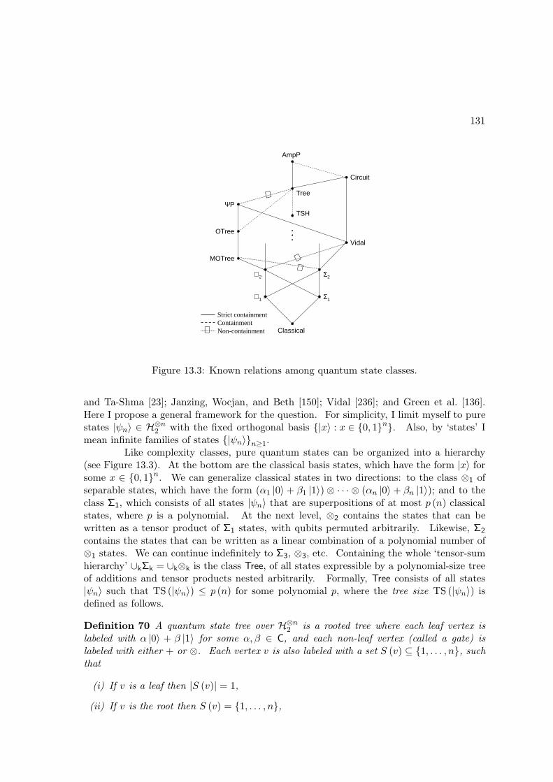
131

Classical

Vidal

Circuit

AmpP

MOTree

OTree

TSH

Tree

ΨP

⊗1

⊗2

Σ1

Σ2

⊄

⊄⊄

Strict containmentContainmentNon-containment⊄

Figure 13.3: Known relations among quantum state classes.

and Ta-Shma [23]; Janzing, Wocjan, and Beth [150]; Vidal [236]; and Green et al. [136].Here I propose a general framework for the question. For simplicity, I limit myself to purestates |ψn〉 ∈ H⊗n

2 with the fixed orthogonal basis |x〉 : x ∈ 0, 1n. Also, by ‘states’ Imean infinite families of states |ψn〉n≥1.

Like complexity classes, pure quantum states can be organized into a hierarchy(see Figure 13.3). At the bottom are the classical basis states, which have the form |x〉 forsome x ∈ 0, 1n. We can generalize classical states in two directions: to the class ⊗1 ofseparable states, which have the form (α1 |0〉 + β1 |1〉) ⊗ · · · ⊗ (αn |0〉 + βn |1〉); and to theclass Σ1, which consists of all states |ψn〉 that are superpositions of at most p (n) classicalstates, where p is a polynomial. At the next level, ⊗2 contains the states that can bewritten as a tensor product of Σ1 states, with qubits permuted arbitrarily. Likewise, Σ2

contains the states that can be written as a linear combination of a polynomial number of⊗1 states. We can continue indefinitely to Σ3, ⊗3, etc. Containing the whole ‘tensor-sumhierarchy’ ∪kΣk = ∪k⊗k is the class Tree, of all states expressible by a polynomial-size treeof additions and tensor products nested arbitrarily. Formally, Tree consists of all states|ψn〉 such that TS (|ψn〉) ≤ p (n) for some polynomial p, where the tree size TS (|ψn〉) isdefined as follows.

Definition 70 A quantum state tree over H⊗n2 is a rooted tree where each leaf vertex is

labeled with α |0〉 + β |1〉 for some α, β ∈ C, and each non-leaf vertex (called a gate) islabeled with either + or ⊗. Each vertex v is also labeled with a set S (v) ⊆ 1, . . . , n, suchthat

(i) If v is a leaf then |S (v)| = 1,

(ii) If v is the root then S (v) = 1, . . . , n,

132

(iii) If v is a + gate and w is a child of v, then S (w) = S (v),

(iv) If v is a ⊗ gate and w1, . . . , wk are the children of v, then S (w1) , . . . , S (wk) arepairwise disjoint and form a partition of S (v).

Finally, if v is a + gate, then the outgoing edges of v are labeled with complexnumbers. For each v, the subtree rooted at v represents a quantum state of the qubits inS (v) in the obvious way. We require this state to be normalized for each v.4

We say a tree is orthogonal if it satisfies the further condition that if v is a +gate, then any two children w1, w2 of v represent |ψ1〉 , |ψ2〉 with 〈ψ1|ψ2〉 = 0. If thecondition 〈ψ1|ψ2〉 = 0 can be replaced by the stronger condition that for all basis states |x〉,either 〈ψ1|x〉 = 0 or 〈ψ2|x〉 = 0, then we say the tree is manifestly orthogonal. Manifestorthogonality is an extremely unphysical definition; I introduce it because it turns out tobe interesting from a lower bounds perspective.

For reasons of convenience, let us define the size |T | of a tree T to be the numberof leaf vertices. Then given a state |ψ〉 ∈ H⊗n

2 , the tree size TS (|ψ〉) is the minimumsize of a tree that represents |ψ〉. The orthogonal tree size OTS (|ψ〉) and manifestlyorthogonal tree size MOTS (|ψ〉) are defined similarly. Then OTree is the class of |ψn〉such that OTS (|ψn〉) ≤ p (n) for some polynomial p, and MOTree is the class such thatMOTS (|ψn〉) ≤ p (n) for some p.

It is easy to see that

n ≤ TS (|ψ〉) ≤ OTS (|ψ〉) ≤ MOTS (|ψ〉) ≤ n2n

for every |ψ〉, and that the set of |ψ〉 such that TS (|ψ〉) < 2n has measure 0 in H⊗n2 . Two

other important properties of TS and OTS are as follows:

Proposition 71

(i) TS and OTS are invariant under local5 basis changes, up to a constant factor of 2.

(ii) If |φ〉 is obtained from |ψ〉 by applying a k-qubit unitary, then TS (|φ〉) ≤ k4k TS (|ψ〉)and OTS (|φ〉) ≤ k4k OTS (|ψ〉).

Proof.

(i) Simply replace each occurrence of |0〉 in the original tree by a tree for α |0〉 + β |1〉,and each occurrence of |1〉 by a tree for γ |0〉 + δ |1〉, as appropriate.

(ii) Suppose without loss of generality that the gate is applied to the first k qubits. LetT be a tree representing |ψ〉, and let Ty be the restriction of T obtained by setting

the first k qubits to y ∈ 0, 1k. Clearly |Ty| ≤ |T |. Furthermore, we can express|φ〉 in the form

∑y∈0,1k SyTy, where each Sy represents a k-qubit state and hence is

expressible by a tree of size k2k.

4Requiring only the whole tree to represent a normalized state clearly yields no further generality.5Several people told me that a reasonable complexity measure must be invariant under all basis changes.

Alas, this would imply that all pure states have the same complexity!

133

One can also define the ε-approximate tree size TSε (|ψ〉) to be the minimum sizeof a tree representing a state |ϕ〉 such that |〈ψ|ϕ〉|2 ≥ 1 − ε, and define OTSε (|ψ〉) andMOTSε (|ψ〉) similarly.

Definition 72 An arithmetic formula (over the ring C and n variables) is a rooted bi-nary tree where each leaf vertex is labeled with either a complex number or a variable inx1, . . . , xn, and each non-leaf vertex is labeled with either + or ×. Such a tree representsa polynomial p (x1, . . . , xn) in the obvious way. We call a polynomial multilinear if novariable appears raised to a higher power than 1, and an arithmetic formula multilinear ifthe polynomials computed by each of its subtrees are multilinear.

The size |Φ| of a multilinear formula Φ is the number of leaf vertices. Given amultilinear polynomial p, the multilinear formula size MFS (p) is the minimum size of amultilinear formula that represents p. Then given a function f : 0, 1n → C, we define

MFS (f) = minp : p(x)=f(x) ∀x∈0,1n

MFS (p) .

(Actually p turns out to be unique [186].) We can also define the ε-approximate multilinearformula size of f ,

MFSε (f) = minp : ‖p−f‖2

2≤εMFS (p)

where ‖p− f‖22 =

∑x∈0,1n |p (x) − f (x)|2. (This metric is closely related to the inner

product∑

x p (x)∗ f (x), but is often more convenient to work with.) Now given a state|ψ〉 =

∑x∈0,1n αx |x〉 in H⊗n

2 , let fψ be the function from 0, 1n to C defined by fψ (x) =αx.

Theorem 73 For all |ψ〉,

(i) MFS (fψ) = O (TS (|ψ〉)).

(ii) TS (|ψ〉) = O (MFS (fψ) + n).

(iii) MFSδ (fψ) = O (TSε (|ψ〉)) where δ = 2 − 2√

1 − ε.

(iv) TS2ε (|ψ〉) = O (MFSε (fψ) + n).

Proof.

(i) Given a tree representing |ψ〉, replace every unbounded fan-in gate by a collection ofbinary gates, every ⊗ by ×, every |1〉i vertex by xi, and every |0〉i vertex by a formulafor 1− xi. Push all multiplications by constants at the edges down to × gates at theleaves.

134

(ii) Given a multilinear formula Φ for fψ, let p (v) be the polynomial computed at vertex vof Φ, and let S (v) be the set of variables that appears in p (v). First, call Φ syntacticif at every × gate with children v and w, S (v) ∩ S (w) = ∅. A lemma of Raz [197]states that we can always make Φ syntactic without increasing its size.

Second, at every + gate u with children v and w, enlarge both S (v) and S (w) toS (v) ∪ S (w), by multiplying p (v) by xi + (1 − xi) for every xi ∈ S (w) \ S (v), andmultiplying p (w) by xi + (1 − xi) for every xi ∈ S (v) \ S (w). Doing this doesnot invalidate any × gate that is an ancestor of u, since by the assumption thatΦ is syntactic, p (u) is never multiplied by any polynomial containing variables inS (v) ∪ S (w). Similarly, enlarge S (r) to x1, . . . , xn where r is the root of Φ.

Third, call v max-linear if |S (v)| = 1 but |S (w)| > 1 where w is the parent of v.If v is max-linear and p (v) = a + bxi, then replace the tree rooted at v by a treecomputing a |0〉i+(a+ b) |1〉i. Also, replace all multiplications by constants higher inΦ by multiplications at the edges. (Because of the second step, there are no additionsby constants higher in Φ.) Replacing every × by ⊗ then gives a tree representing|ψ〉, whose size is easily seen to be O (|Φ| + n) .

(iii) Apply the reduction from part (i). Let the resulting multilinear formula computepolynomial p; then

∑

x∈0,1n

|p (x) − fψ (x)|2 = 2 − 2∑

x∈0,1n

p (x) fψ (x) ≤ 2 − 2√

1 − ε = δ.

(iv) Apply the reduction from part (ii). Let (βx)x∈0,1n be the resulting amplitude vector;

since this vector might not be normalized, divide each βx by∑

x |βx|2 to produce β′x.Then

∣∣∣∣∣∣

∑

x∈0,1n

β′xαx

∣∣∣∣∣∣

2

= 1 − 1

2

∑

x∈0,1n

∣∣β′x − αx∣∣2

≥ 1 − 1

2

√ ∑

x∈0,1n

|β′x − βx|2 +

√ ∑

x∈0,1n

|βx − αx|2

2

≥ 1 − 1

2

(2√ε)2

= 1 − 2ε.

Besides Tree, OTree, and MOTree, four other classes of quantum states deservemention:

Circuit, a circuit analog of Tree, contains the states |ψn〉 =∑

x αx |x〉 such that forall n, there exists a multilinear arithmetic circuit of size p (n) over the complex numbersthat outputs αx given x as input, for some polynomial p. (Multilinear circuits are thesame as multilinear trees, except that they allow unbounded fanout—that is, polynomialscomputed at intermediate points can be reused arbitrarily many times.)

135

AmpP contains the states |ψn〉 =∑

x αx |x〉 such that for all n, b, there exists aclassical circuit of size p (n+ b) that outputs αx to b bits of precision given x as input, forsome polynomial p.

Vidal contains the states that are ‘polynomially entangled’ in the sense of Vidal[236]. Given a partition of 1, . . . , n into A and B, let χA (|ψn〉) be the minimum kfor which |ψn〉 can be written as

∑ki=1 αi

∣∣ϕAi⟩⊗∣∣ϕBi

⟩, where

∣∣ϕAi⟩

and∣∣ϕBi

⟩are states of

qubits in A and B respectively. (χA (|ψn〉) is known as the Schmidt rank ; see [184] formore information.) Let χ (|ψn〉) = maxA χA (|ψn〉). Then |ψn〉 ∈ Vidal if and only ifχ (|ψn〉) ≤ p (n) for some polynomial p.

ΨP contains the states |ψn〉 such that for all n and ε > 0, there exists a quantumcircuit of size p (n+ log (1/ε)) that maps the all-0 state to a state some part of which hastrace distance at most 1−ε from |ψn〉, for some polynomial p. Because of the Solovay-KitaevTheorem [155, 184], ΨP is invariant under the choice of universal gate set.

13.3 Basic Results

Before studying the tree size of specific quantum states, it would be nice to know in generalhow tree size behaves as a complexity measure. In this section I prove three rather niceproperties of tree size.

Theorem 74 For all ε > 0, there exists a tree representing |ψ〉 of size O(TS (|ψ〉)1+ε

)and

depth O (log TS (|ψ〉)), as well as a manifestly orthogonal tree of size O(MOTS (|ψ〉)1+ε

)

and depth O (log MOTS (|ψ〉)).

Proof. A classical theorem of Brent [70] says that given an arithmetic formulaΦ, there exists an equivalent formula of depth O (log |Φ|) and size O (|Φ|c), where c is aconstant. Bshouty, Cleve, and Eberly [73] (see also Bonet and Buss [62]) improved Brent’stheorem to show that c can be taken to be 1 + ε for any ε > 0. So it suffices to show that,for ‘division-free’ formulas, these theorems preserve multilinearity (and in the MOTS case,preserve manifest orthogonality).

Brent’s theorem is proven by induction on |Φ|. Here is a sketch: choose a sub-formula I of Φ size between |Φ| /3 and 2 |Φ| /3 (which one can show always exists). Thenidentifying a subformula with the polynomial computed at its root, Φ (x) can be written asG (x)+H (x) I (x) for some formulas G and H. Furthermore, G and H are both obtainablefrom Φ by removing I and then applying further restrictions. So |G| and |H| are both atmost |Φ| − |I| + O (1). Let Φ be a formula equivalent to Φ that evaluates G, H, and I

separately, and then returns G (x) +H (x) I (x). Then∣∣∣Φ∣∣∣ is larger than |Φ| by at most a

constant factor, while by the induction hypothesis, we can assume the formulas for G, H,and I have logarithmic depth. Since the number of induction steps is O (log |Φ|), the totaldepth is logarithmic and the total blowup in formula size is polynomial in |Φ|. Bshouty,Cleve, and Eberly’s improvement uses a more careful decomposition of Φ, but the basicidea is the same.

Now, if Φ is syntactic multilinear, then clearly G, H, and I are also syntacticmultilinear. Furthermore, H cannot share variables with I, since otherwise a subformula

136

of Φ containing I would have been multiplied by a subformula containing variables from I.Thus multilinearity is preserved. To see that manifest orthogonality is preserved, supposewe are evaluating G and H ‘bottom up,’ and let Gv and Hv be the polynomials computedat vertex v of Φ. Let v0 = root (I), let v1 be the parent of v0, let v2 be the parent of v1, andso on until vk = root (Φ). It is clear that, for every x, either Gv0 (x) = 0 or Hv0 (x) = 0.Furthermore, suppose that property holds for Gvi−1 ,Hvi−1 ; then by induction it holds forGvi ,Hvi . If vi is a × gate, then this follows from multilinearity (if |ψ〉 and |ϕ〉 are manifestlyorthogonal, then |0〉 ⊗ |ψ〉 and |0〉 ⊗ |ϕ〉 are also manifestly orthogonal). If vi is a + gate,then letting supp (p) be the set of x such that p (x) 6= 0, any polynomial p added to Gvi−1

or Hvi−1 must have

supp (p) ∩(supp

(Gvi−1

)∪ supp

(Hvi−1

))= ∅,

and manifest orthogonality follows.

Theorem 75 Any |ψ〉 can be prepared by a quantum circuit of size polynomial in OTS (|ψ〉).Thus OTree ⊆ ΨP.

Proof. Let Γ (|ψ〉) be the minimum size of a circuit needed to prepare |ψ〉 ∈ H⊗n2

starting from |0〉⊗n. The claim, by induction on Γ (|ψ〉), is that Γ (|ψ〉) ≤ q (OTS (|ψ〉))for some polynomial q. The base case OTS (|ψ〉) = 1 is clear. Let T be an orthogonalstate tree for |ψ〉, and assume without loss of generality that every gate has fan-in 2 (thisincreases |T | by at most a constant factor). Let T1 and T2 be the subtrees of root (T ),representing states |ψ1〉 and |ψ2〉 respectively; note that |T | = |T1| + |T2|. First supposeroot (T ) is a ⊗ gate; then clearly Γ (|ψ〉) ≤ Γ (|ψ1〉) + Γ (|ψ2〉).

Second, suppose root (T ) is a + gate, with |ψ〉 = α |ψ1〉 + β |ψ2〉 and 〈ψ1|ψ2〉 =0. Let U be a quantum circuit that prepares |ψ1〉, and V be a circuit that prepares|ψ2〉. Then we can prepare α |0〉 |0〉⊗n + β |1〉U−1V |0〉⊗n. Observe that U−1V |0〉⊗n isorthogonal to |0〉⊗n, since |ψ1〉 = U |0〉⊗n is orthogonal to |ψ2〉 = V |0〉⊗n. So applyinga NOT to the first register, conditioned on the OR of the bits in the second register,yields |0〉 ⊗

(α |0〉⊗n + βU−1V |0〉⊗n

), from which we obtain α |ψ1〉 + β |ψ2〉 by applying U

to the second register. The size of the circuit used is O (|U | + |V | + n), with a possibleconstant-factor blowup arising from the need to condition on the first register. If we aremore careful, however, we can combine the ‘conditioning’ steps across multiple levels of therecursion, producing a circuit of size |V | +O (|U | + n). By symmetry, we can also reversethe roles of U and V to obtain a circuit of size |U | +O (|V | + n). Therefore

Γ (|ψ〉) ≤ min Γ (|ψ1〉) + cΓ (|ψ2〉) + cn, cΓ (|ψ2〉) + Γ (|ψ1〉) + cn

for some constant c ≥ 2. Solving this recurrence we find that Γ (|ψ〉) is polynomial inOTS (|ψ〉).

Theorem 76 If |ψ〉 ∈ H⊗n2 is chosen uniformly at random under the Haar measure, then

TS1/16 (|ψ〉) = 2Ω(n) with probability 1 − o (1).

137

Proof. To generate a uniform random state |ψ〉 =∑

x∈0,1n αx |x〉, we can choose

αx, βx ∈ R for each x independently from a Gaussian distribution with mean 0 and variance

1, then let αx =(αx + iβx

)/√R where R =

∑x∈0,1n

(α2x + β2

x

). Let

Λψ =

x : (Reαx)

2 <1

4 · 2n,

and let G be the set of |ψ〉 for which |Λψ| < 2n/5. The claim is that Pr|ψ〉 [|ψ〉 ∈ G] =1 − o (1). First, EX [R] = 2n+1, so by a standard Hoeffding-type bound, Pr [R < 2n] isdoubly-exponentially small in n. Second, assuming R ≥ 2n, for each x

Pr [x ∈ Λψ] ≤ Pr

[α2x <

1

4

]= erf

(1

4√

2

)< 0.198,

and the claim follows by a Chernoff bound.For g : 0, 1n → R, let Ag = x : sgn (g (x)) 6= sgn (Reαx), where sgn (y) is 1 if

y ≥ 0 and −1 otherwise. Then if |ψ〉 ∈ G, clearly

∑

x∈0,1n

|g (x) − fψ (x)|2 ≥ |Ag| − |Λψ|4 · 2n

where fψ (x) = Reαx, and thus

|Ag| ≤(

4 ‖g − fψ‖22 +

1

5

)2n.

Therefore to show that MFS1/15 (fψ) = 2Ω(n) with probability 1− o (1), we need only showthat for almost all Boolean functions f : 0, 1n → −1, 1, there is no arithmetic formulaΦ of size 2o(n) such that

|x : sgn (Φ (x)) 6= f (x)| ≤ 0.49 · 2n.

Here an arithmetic formula is real-valued, and can include addition, subtraction, and mul-tiplication gates of fan-in 2 as well as constants. We do not need to assume multilinearity,and it is easy to see that the assumption of bounded fan-in is without loss of generality. LetW be the set of Boolean functions sign-represented by an arithmetic formula Φ of size 2o(n),in the sense that sgn (Φ (x)) = f (x) for all x. Then it suffices to show that |W | = 22o(n)

,since the number of functions sign-represented on an 0.51 fraction of inputs is at most|W | · 22nH(0.51). (Here H denotes the binary entropy function.)

Let Φ be an arithmetic formula that takes as input the binary string x = (x1, . . . , xn)as well as constants c1, c2, . . .. Let Φc denote Φ under a particular assignment c to c1, c2, . . ..Then a result of Gashkov [123] (see also Turan and Vatan [232]), which follows from War-ren’s Theorem [237] in real algebraic geometry, shows that as we range over all c, Φc

sign-represents at most(2n+4 |Φ|

)|Φ|distinct Boolean functions, where |Φ| is the size of Φ.

Furthermore, excluding constants, the number of distinct arithmetic formulas of size |Φ| is

138

at most(3 |Φ|2

)|Φ|. When |Φ| = 2o(n), this gives

(3 |Φ|2

)|Φ|·(2n+4 |Φ|

)|Φ|= 22o(n)

. There-

fore MFS1/15 (fψ) = 2Ω(n); by Theorem 73, part (iii), this implies that TS1/16 (|ψ〉) = 2Ω(n).

A corollary of Theorem 76 is the following ‘nonamplification’ property: there existstates that can be approximated to within, say, 1% by trees of polynomial size, but thatrequire exponentially large trees to approximate to within a smaller margin (say 0.01%).

Corollary 77 For all δ ∈ (0, 1], there exists a state |ψ〉 such that TSδ (|ψ〉) = n butTSε (|ψ〉) = 2Ω(n) where ε = δ/32 − δ2/4096.

Proof. It is clear from Theorem 76 that there exists a state |ϕ〉 =∑

x∈0,1n αx |x〉such that TS1/16 (|ϕ〉) = 2Ω(n) and α0n = 0. Take |ψ〉 =

√1 − δ |0〉⊗n +

√δ |ϕ〉. Since∣∣〈ψ|0〉⊗n

∣∣2 = 1 − δ, we have MOTSδ (|ψ〉) = n. On the other hand, suppose some |φ〉 =∑x∈0,1n βx |x〉 with TS (|φ〉) = 2o(n) satisfies |〈φ|ψ〉|2 ≥ 1 − ε. Then

∑

x 6=0n

(√δαx − βx

)2≤ 2 − 2

√1 − ε.

Thus, letting fϕ (x) = αx, we have MFSc (fϕ) = O (TS (|φ〉)) where c =(2 − 2

√1 − ε

)/δ.

By Theorem 73, part (iv), this implies that TS2c (|ϕ〉) = O (TS (|φ〉)). But 2c = 1/16 whenε = δ/32 − δ2/4096, contradiction.

13.4 Relations Among Quantum State Classes

This section presents some results about the quantum state hierarchy introduced in Section13.2. Theorem 78 shows simple inclusions and separations, while Theorem 79 shows thatseparations higher in the hierarchy would imply major complexity class separations (andvice versa).

Theorem 78

(i) Tree ∪ Vidal ⊆ Circuit ⊆ AmpP.

(ii) All states in Vidal have tree size nO(logn).

(iii) Σ2 ⊆ Vidal but ⊗2 6⊂ Vidal.

(iv) ⊗2 ( MOTree.

(v) Σ1, Σ2, Σ3, ⊗1, ⊗2, and ⊗3 are all distinct. Also, ⊗3 6= Σ4 ∩ ⊗4.

Proof.

139

(i) Tree ⊆ Circuit since any multilinear tree is also a multilinear circuit. Circuit ⊆ AmpP

since the circuit yields a polynomial-time algorithm for computing the amplitudes.For Vidal ⊆ Circuit, we use an idea of Vidal [236]: given |ψn〉 ∈ Vidal, for all j ∈1, . . . , n we can express |ψn〉 as

χ(|ψ〉)∑

i=1

αij

∣∣∣φ[1...j]i

⟩⊗∣∣∣φ[j+1...n]i

⟩

where χ (|ψn〉) is polynomially bounded. Furthermore, Vidal showed that each∣∣∣φ[1...j]i

⟩can be written as a linear combination of states of the form

∣∣∣φ[1...j−1]i

⟩⊗ |0〉

and∣∣∣φ[1...j−1]i

⟩⊗ |1〉—the point being that the set of

∣∣∣φ[1...j−1]i

⟩states is the same, in-

dependently of∣∣∣φ[1...j]i

⟩. This immediately yields a polynomial-size multilinear circuit

for |ψn〉.

(ii) Given |ψn〉 ∈ Vidal, we can decompose |ψn〉 as

χ(|ψ〉)∑

i=1

αi

∣∣∣φ[1...n/2]i

⟩⊗∣∣∣φ[n/2+1...n]i

⟩.

Then χ(∣∣∣φ[1...n/2]

i

⟩)≤ χ (|ψn〉) and χ

(∣∣∣φ[n/2+1...n]i

⟩)≤ χ (|ψn〉) for all i, so we can

recursively decompose these states in the same manner. It follows that TS (|ψn〉) ≤2χ (|ψ〉) TS

(∣∣ψn/2⟩)

; solving this recurrence relation yields TS (|ψn〉) ≤ (2χ (|ψ〉))logn =

nO(logn).

(iii) Σ2 ⊆ Vidal follows since a sum of t separable states has χ ≤ t, while ⊗2 6⊂ Vidal follows

from the example of n/2 Bell pairs: 2−n/4 (|00〉 + |11〉)⊗n/2.

(iv) ⊗2 ⊆ MOTree is obvious, while MOTree 6⊂ ⊗2 follows from the example of∣∣P in⟩, an

equal superposition over all n-bit strings of parity i. The following recursive formulas

imply that MOTS(∣∣P in

⟩)≤ 4MOTS

(∣∣∣P in/2⟩)

= O(n2):

∣∣P 0n

⟩=

1√2

(∣∣∣P 0n/2

⟩ ∣∣∣P 0n/2

⟩+∣∣∣P 1n/2

⟩ ∣∣∣P 1n/2

⟩),

∣∣P 1n

⟩=

1√2

(∣∣∣P 0n/2

⟩ ∣∣∣P 1n/2

⟩+∣∣∣P 1n/2

⟩ ∣∣∣P 0n/2

⟩).

On the other hand, |Pn〉 /∈ ⊗2 follows from |Pn〉 /∈ Σ1 together with the fact that |Pn〉has no nontrivial tensor product decomposition.

(v) ⊗1 6⊂ Σ1 and Σ1 6⊂ ⊗1 are obvious. ⊗2 6⊂ Σ2 (and hence ⊗1 6= ⊗2) follows from part(iii). Σ2 6⊂ ⊗2 (and hence Σ1 6= Σ2) follows from part (iv), together with the factthat |Pn〉 has a Σ2 formula based on the Fourier transform:

|Pn〉 =1√2

(( |0〉 + |1〉√2

)⊗n+

( |0〉 − |1〉√2

)⊗n).

140

Σ2 6= Σ3 follows from ⊗2 6⊂ Σ2 and ⊗2 ⊆ Σ3. Also, Σ3 6⊂ ⊗3 follows from Σ2 6= Σ3,together with the fact that we can easily construct states in Σ3 \ Σ2 that have nonontrivial tensor product decomposition—for example,

1√2

(|0〉⊗n +

( |01〉 + |10〉√2

)⊗n/2).

⊗2 6= ⊗3 follows from Σ2 6⊂ ⊗2 and Σ2 ⊆ ⊗3. Finally, ⊗3 6= Σ4 ∩ ⊗4 follows fromΣ3 6⊂ ⊗3 and Σ3 ⊆ Σ4 ∩ ⊗4.

Theorem 79

(i) BQP = P#P implies AmpP ⊆ ΨP.

(ii) AmpP ⊆ ΨP implies NP ⊆ BQP/poly.

(iii) P = P#P implies ΨP ⊆ AmpP.

(iv) ΨP ⊆ AmpP implies BQP ⊆ P/poly.

Proof.

(i) First, BQP = P#P implies BQP/poly = P#P/poly, since given a P#P/poly machineM , the language consisting of all (x, a) such that M accepts on input x and advicea is clearly in BQP. So assume BQP/poly = P#P/poly, and consider a state |ψ〉 =∑

x∈0,1n αx |x〉 with |ψ〉 ∈ AmpP. By the result of Bernstein and Vazirani [55] that

BQP ⊆ P#P, for all b there exists a quantum circuit of size polynomial in n and bthat approximates p0 =

∑y∈0,1n−1 |α0y|2, or the probability that the first qubit is

measured to be 0, to b bits of precision. So by uncomputing garbage, we can preparea state close to

√p0 |0〉 +

√1 − p0 |1〉. Similarly, given a superposition over length-

k prefixes of x, we can prepare a superposition over length-(k + 1) prefixes of x byapproximating the conditional measurement probabilities. We thus obtain a stateclose to

∑x |αx| |x〉. The last step is to approximate the phase of each |x〉, apply that

phase, and uncompute to obtain a state close to∑

x αx |x〉.

(ii) Given a SAT instance ϕ, first use Valiant-Vazirani [233] to produce a formula ϕ′ that(with non-negligible probability) has one satisfying assignment if ϕ is satisfiable andzero otherwise. Then let αx = 1 if x is a satisfying assignment for ϕ′ and αx = 0otherwise; clearly |ψ〉 =

∑x αx |x〉 is in AmpP. By the assumption AmpP ⊆ ΨP, there

exists a polynomial-size quantum circuit that approximates |ψ〉, and thereby finds theunique satisfying assignment for ϕ′ if it exists.

(iii) As in part (i), P = P#P implies P/poly = P#P/poly. The containment ΨP ⊆ AmpP

follows since we can approximate amplitudes to polynomially many bits of precisionin #P.

141

(iv) As is well known [55], any quantum computation can be made ‘clean’ in the sensethat it accepts if and only if a particular basis state (say |0〉⊗n) is measured. Theimplication follows easily.

13.5 Lower Bounds

We want to show that certain quantum states of interest to us are not represented by treesof polynomial size. At first this seems like a hopeless task. Proving superpolynomialformula-size lower bounds for ‘explicit’ functions is a notoriously hard open problem, as itwould imply complexity class separations such as NC1 6= P.

Here, though, we are only concerned with multilinear formulas. Could this makeit easier to prove a lower bound? The answer is not obvious, but very recently, for reasonsunrelated to quantum computing, Raz [197, 198] showed the first superpolynomial lowerbounds on multilinear formula size. In particular, he showed that multilinear formulascomputing the permanent or determinant of an n×n matrix over any field have size nΩ(logn).

Raz’s technique is a beautiful combination of the Furst-Saxe-Sipser method of ran-dom restrictions [122], with matrix rank arguments as used in communication complexity.I now outline the method. Given a function f : 0, 1n → C, let P be a partition of theinput variables x1, . . . , xn into two collections y =

(y1, . . . , yn/2

)and z =

(z1, . . . , zn/2

).

This yields a function fP (y, z) : 0, 1n/2 ×0, 1n/2 → C. Then let Mf |P be a 2n/2 × 2n/2

matrix whose rows are labeled by assignments y ∈ 0, 1n/2, and whose columns are labeled

by assignments z ∈ 0, 1n/2. The (y, z) entry of Mf |P is fP (y, z). Let rank(Mf |P

)be

the rank of Mf |P over the complex numbers. Finally, let P be the uniform distributionover all partitions P .

The following, Corollary 3.6 in [198], is one statement of Raz’s main theorem;recall that MFS (f) is the minimum size of a multilinear formula for f .

Theorem 80 ([198]) Suppose that

PrP∈P

[rank

(Mf |P

)≥ 2n/2−(n/2)1/8/2

]= n−o(logn).

Then MFS (f) = nΩ(logn).

An immediate corollary yields lower bounds on approximate multilinear formulasize. Given an N ×N matrix M = (mij), let rankε (M) = minL : ‖L−M‖2

2≤ε rank (L) where

‖L−M‖22 =

∑Ni,j=1 |`ij −mij|2.

Corollary 81 Suppose that

PrP∈P

[rankε

(Mf |P

)≥ 2n/2−(n/2)1/8/2

]= n−o(logn).

Then MFSε (f) = nΩ(logn).

142

Proof. Suppose MFSε (f) = no(logn). Then for all g such that ‖f − g‖22 ≤ ε, we

would have MFS (g) = no(logn), and therefore

PrP∈P

[rank

(Mg|P

)≥ 2n/2−(n/2)1/8/2

]= n−Ω(logn).

by Theorem 80. But rankε(Mf |P

)≤ rank

(Mg|P

), and hence

PrP∈P

[rankε

(Mf |P

)≥ 2n/2−(n/2)1/8/2

]= n−Ω(logn),

contradiction.Another simple corollary gives lower bounds in terms of restrictions of f . Let

R` be the following distribution over restrictions R: choose 2` variables of f uniformly atrandom, and rename them y = (y1, . . . , y`) and z = (z1, . . . , z`). Set each of the remainingn− 2` variables to 0 or 1 uniformly and independently at random. This yields a restrictedfunction fR (y, z). Let Mf |R be a 2` × 2` matrix whose (y, z) entry is fR (y, z).

Corollary 82 Suppose that

PrR∈R`

[rank

(Mf |R

)≥ 2`−`

1/8/2]

= n−o(logn)

where ` = nδ for some constant δ ∈ (0, 1]. Then MFS (f) = nΩ(logn).

Proof. Under the hypothesis, clearly there exists a fixed restriction g : 0, 12` →C of f , which leaves 2` variables unrestricted, such that

PrP∈P

[rank

(Mg|P

)≥ 2`−`

1/8/2]

= n−o(logn) = `−o(log `).

Then by Theorem 80,

MFS (f) ≥ MFS (g) = `Ω(log `) = nΩ(logn).

The following sections apply Raz’s theorem to obtain nΩ(logn) tree size lowerbounds for two classes of quantum states: states arising in quantum error-correction inSection 13.5.1, and (assuming a number-theoretic conjecture) states arising in Shor’s fac-toring algorithm in Section 13.5.2.

13.5.1 Subgroup States

Let the elements of Zn2 be labeled by n-bit strings. Given a subgroup S ≤ Zn2 , we definethe subgroup state |S〉 as follows:

|S〉 =1√|S|∑

x∈S|x〉 .

143

Coset states arise as codewords in the class of quantum error-correcting codes known asstabilizer codes [80, 135, 227]. Our interest in these states, however, arises from their largetree size rather than their error-correcting properties.

Let E be the following distribution over subgroups S. Choose an n/2 × n ma-trix A by setting each entry to 0 or 1 uniformly and independently. Then let S =x | Ax ≡ 0 (mod 2). By Theorem 73, part (i), it suffices to lower-bound the multilin-ear formula size of the function fS (x), which is 1 if x ∈ S and 0 otherwise.

Theorem 83 If S is drawn from E, then MFS (fS) = nΩ(logn) (and hence TS (|S〉) =nΩ(logn)), with probability Ω (1) over S.

Proof. Let P be a uniform random partition of the inputs x1, . . . , xn of fS intotwo sets y =

(y1, . . . , yn/2

)and z =

(z1, . . . , zn/2

). Let MS|P be the 2n/2 × 2n/2 matrix

whose (y, z) entry is fS|P (y, z); then we need to show that rank(MS|P

)is large with high

probability. Let Ay be the n/2 × n/2 submatrix of the n/2 × n matrix A consistingof all rows that correspond to yi for some i ∈ 1, . . . , n/2, and similarly let Az be then/2 × n/2 submatrix corresponding to z. Then it is easy to see that, so long as Ay andAz are both invertible, for all 2n/2 settings of y there exists a unique setting of z for whichfS|P (y, z) = 1. This then implies that MS|P is a permutation of the identity matrix, and

hence that rank(MS|P

)= 2n/2. Now, the probability that a random n/2 × n/2 matrix

over Z2 is invertible is1

2· 3

4· · · · · 2n/2 − 1

2n/2> 0.288.

So the probability that Ay and Az are both invertible is at least 0.2882. By Markov’sinequality, it follows that for at least an 0.04 fraction of S’s, rank

(MS|P

)= 2n/2 for at least

an 0.04 fraction of P ’s. Theorem 80 then yields the desired result.Aaronson and Gottesman [14] showed how to prepare any n-qubit subgroup state

using a quantum circuit of size O(n2/ log n

). So a corollary of Theorem 83 is that ΨP 6⊂

Tree. Since fS clearly has a (non-multilinear) arithmetic formula of size O (nk), a secondcorollary is the following.

Corollary 84 There exists a family of functions fn : 0, 1n → R that has polynomial-sizearithmetic formulas, but no polynomial-size multilinear formulas.

The reason Corollary 84 does not follow from Raz’s results is that polynomial-sizeformulas for the permanent and determinant are not known; the smallest known formulasfor the determinant have size nO(logn) (see [79]).

We have shown that not all subgroup states are tree states, but it is still conceivablethat all subgroup states are extremely well approximated by tree states. Let us now ruleout the latter possibility. We first need a lemma about matrix rank, which follows fromthe Hoffman-Wielandt inequality.

Lemma 85 Let M be an N ×N complex matrix, and let IN be the N ×N identity matrix.Then ‖M − IN‖2

2 ≥ N − rank (M).

144

Proof. The Hoffman-Wielandt inequality [146] (see also [33]) states that for anytwo N ×N matrices M,P ,

N∑

i=1

(σi (M) − σi (P ))2 ≤ ‖M − P‖22 ,

where σi (M) is the ith singular value of M (that is, σi (M) =√λi (M), where λ1 (M) ≥

· · · ≥ λN (M) ≥ 0 are the eigenvalues of MM∗, and M∗ is the conjugate transpose of M).Clearly σi (IN ) = 1 for all i. On the other hand, M has only rank (M) nonzero singularvalues, so

N∑

i=1

(σi (M) − σi (IN ))2 ≥ N − rank (M) .

Let fS (x) = fS (x) /√

|S| be fS (x) normalized to have∥∥∥fS

∥∥∥2

2= 1.

Theorem 86 For all constants ε ∈ [0, 1), if S is drawn from E, then MFSε

(fS

)= nΩ(logn)

with probability Ω (1) over S.

Proof. As in Theorem 83, we look at the matrix MS|P induced by a randompartition P = (y, z). We already know that for at least an 0.04 fraction of S’s, the y andz variables are in one-to-one correspondence for at least an 0.04 fraction of P ’s. In thatcase |S| = 2n/2, and therefore MS|P is a permutation of I/

√|S| = I/2n/4 where I is the

identity. It follows from Lemma 85 that for all matrices M such that∥∥M −MS|P

∥∥2

2≤ ε,

rank (M) ≥ 2n/2 −∥∥∥√|S|(M −MS|P

)∥∥∥2

2≥ (1 − ε) 2n/2

and therefore rankε(MS|P

)≥ (1 − ε) 2n/2. Hence

PrP∈P

[rankε

(Mf |P

)≥ 2n/2−(n/2)1/8/2

]≥ 0.04,

and the result follows from Corollary 81.A corollary of Theorem 86 and of Theorem 73, part (iii), is that TSε (|S〉) =

nΩ(logn) with probability Ω (1) over S, for all ε < 1.Finally, let me show how to derandomize the lower bound for subgroup states,

using ideas pointed out to me by Andrej Bogdanov. In the proof of Theorem 83, all weneeded about the matrix A was that a random k × k submatrix has full rank with Ω (1)probability, where k = n/2. If we switch from the field F2 to F2d for some d ≥ log2 n, thenit is easy to construct explicit k × n matrices with this same property. For example, let

V =

10 11 · · · 1k−1

20 21 · · · 2k−1

......

...n0 n1 · · · nk−1

145

be the n× k Vandermonde matrix, where 1, . . . , n are labels of elements in F2d . Any k× ksubmatrix of V has full rank, because the Reed-Solomon (RS) code that V represents isa perfect erasure code.6 Hence, there exists an explicit state of n “qupits” with p = 2d

that has tree size nΩ(logn)—namely the uniform superposition over all elements of the setx | V Tx = 0

, where V T is the transpose of V .

To replace qupits by qubits, we concatenate the RS and Hadamard codes to obtaina binary linear erasure code with parameters almost as good as those of the original RScode. More explicitly, interpret F2d as the field of polynomials over F2, modulo someirreducible of degree d. Then let m (a) be the d× d Boolean matrix that maps q ∈ F2d toaq ∈ F2d , where q and aq are encoded by their d × 1 vectors of coefficients. Let H mapa length-d vector to its length-2d Hadamard encoding. Then Hm (a) is a 2d × d Booleanmatrix that maps q ∈ F2d to the Hadamard encoding of aq. We can now define an n2d×kd“binary Vandermonde matrix” as follows:

Vbin =

Hm(10)

Hm(11)

· · · Hm(1k−1

)

Hm(20)

Hm(21)

· · · Hm(2k−1

)...

......

Hm(n0)

Hm(n1)

· · · Hm(nk−1

)

.

For the remainder of the section, fix k = nδ for some δ < 1/2 and d = O (log n).

Lemma 87 A (kd+ c) × kd submatrix of Vbin chosen uniformly at random has rank kd(that is, full rank) with probability at least 2/3, for c a sufficiently large constant.

Proof. The first claim is that |Vbinu| ≥ (n− k) 2d−1 for all nonzero vectors u ∈Fkd2 , where | | represents the number of ‘1’ bits. To see this, observe that for all nonzero u,the “codeword vector” V u ∈ Fn

2d must have at least n−k nonzero entries by the Fundamental

Theorem of Algebra, where here u is interpreted as an element of Fk2d . Furthermore, the

Hadamard code maps any nonzero entry in V u to 2d−1 nonzero bits in Vbinu ∈ Fn2d

2 .Now let W be a uniformly random (kd+ c)× kd submatrix of Vbin. By the above

claim, for any fixed nonzero vector u ∈ Fkd2 ,

PrW

[Wu = 0] ≤(

1 − (n− k) 2d−1

n2d

)kd+c=

(1

2+

k

2n

)kd+c.

So by the union bound, Wu is nonzero for all nonzero u (and hence W is full rank) withprobability at least

1 − 2kd(

1

2+

k

2n

)kd+c= 1 −

(1 +

k

n

)kd(1

2+

k

2n

)c.

Since k = n1/2−Ω(1) and d = O (log n), the above quantity is at least 2/3 for sufficientlylarge c.

Given an n2d × 1 Boolean vector x, let f (x) = 1 if V Tbinx = 0 and f (x) = 0

otherwise. Then:6In other words, because a degree-(k − 1) polynomial is determined by its values at any k points.

146

Theorem 88 MFS (f) = nΩ(logn).

Proof. Let Vy and Vz be two disjoint kd × (kd+ c) submatrices of V Tbin chosen

uniformly at random. Then by Lemma 87 together with the union bound, Vy and Vz bothhave full rank with probability at least 1/3. Letting ` = kd+ c, it follows that

PrR∈R`

[rank

(Mf |R

)≥ 2`−c

]≥ 1

3= n−o(logn)

by the same reasoning as in Theorem 83. Therefore MFS (f) = nΩ(logn) by Corollary 82.

Let |S〉 be a uniform superposition over all x such that f (x) = 1; then a corollaryof Theorem 88 is that TS (|S〉) = nΩ(logn). Naturally, using the ideas of Theorem 86 onecan also show that TSε (|S〉) = nΩ(logn) for all ε < 1.

13.5.2 Shor States

Since the motivation for this work was to study possible Sure/Shor separators, an obviousquestion is, do states arising in Shor’s algorithm have superpolynomial tree size? Unfortu-nately, I am only able to answer this question assuming a number-theoretic conjecture. Toformalize the question, let

1

2n/2

2n−1∑

r=0

|r〉 |xr modN〉

be a Shor state. It will be convenient to measure the second register, so that the state ofthe first register has the form

|a+ pZ〉 =1√I

I∑

i=0

|a+ pi〉

for some integers a < p and I = b(2n − a− 1) /pc. Here a+pi is written out in binary usingn bits. Clearly a lower bound on TS (|a+ pZ〉) would imply an equivalent lower bound forthe joint state of the two registers.

To avoid some technicalities, assume p is prime (since the goal is to prove a lowerbound, this assumption is without loss of generality). Given an n-bit string x = xn−1 . . . x0,let fn,p,a (x) = 1 if x ≡ a (mod p) and fn,p,a (x) = 0 otherwise. Then TS (|a+ pZ〉) =Θ (MFS (fn,p,a)) by Theorem 73, so from now on we will focus attention on fn,p,a.

Proposition 89

(i) Let fn,p = fn,p,0. Then MFS (fn,p,a) ≤ MFS (fn+log p,p), meaning that we can seta = 0 without loss of generality.

(ii) MFS (fn,p) = O (min n2n/p, np).

Proof.

147

(i) Take the formula for fn+log p,p, and restrict the most significant log p bits to sumto a number congruent to −amod p (this is always possible since x → 2nx is anisomorphism of Zp).

(ii) For MFS (fn,p) = O (n2n/p), write out the x’s for which fn,p (x) = 1 explicitly. ForMFS (fn,p) = O (np), use the Fourier transform, similarly to Theorem 78, part (v):

fn,p (x) =1

p

p−1∑

h=0

n−1∏

j=0

exp

(2πih

p· 2jxj

).

This immediately yields a sum-of-products formula of size O (np).

I now state the number-theoretic conjecture.

Conjecture 90 There exist constants γ, δ ∈ (0, 1) and a prime p = Ω(2n

δ)

for which the

following holds. Let the set A consist of nδ elements of20, . . . , 2n−1

chosen uniformly at

random. Let S consist of all 2nδ

sums of subsets of A, and let Smod p = xmod p : x ∈ S.Then

PrA

[|Smod p| ≥ (1 + γ)

p

2

]= n−o(logn).

Theorem 91 Conjecture 90 implies that MFS (fn,p) = nΩ(logn) and hence TS (|pZ〉) =nΩ(logn).

Proof. Let f = fn,p and ` = nδ. Let R be a restriction of f that renames 2`variables y1, . . . , y`, z1, . . . , z`, and sets each of the remaining n−2` variables to 0 or 1. Thisleads to a new function, fR (y, z), which is 1 if y + z + c ≡ 0 (mod p) and 0 otherwise forsome constant c. Here we are defining y = 2a1y1 + · · · + 2a`y` and z = 2b1z1 + · · · + 2b`z`where a1, . . . , a`, b1, . . . , b` are the appropriate place values. Now suppose ymod p andzmod p both assume at least (1 + γ) p/2 distinct values as we range over all x ∈ 0, 1n.Then by the pigeonhole principle, for at least γp possible values of ymod p, there exists aunique possible value of zmod p for which y + z + c ≡ 0 (mod p) and hence fR (y, z) = 1.So rank

(Mf |R

)≥ γp, where Mf |R is the 2` × 2` matrix whose (y, z) entry is fR (y, z). It

follows that assuming Conjecture 90,

PrR∈R`

[rank

(Mf |R

)≥ γp

]= n−o(logn).

Furthermore, γp ≥ 2`−`1/8/2 for sufficiently large n since p = Ω

(2n

δ). Therefore MFS (f) =

nΩ(logn) by Corollary 82.Using the ideas of Theorem 86, one can show that under the same conjecture,

MFSε (fn,p) = nΩ(logn) and TSε (|pZ〉) = nΩ(logn) for all ε < 1—in other words, there existShor states that cannot be approximated by polynomial-size trees.

Originally, I had stated Conjecture 90 without any restriction on how the set Sis formed. The resulting conjecture was far more general than I needed, and indeed wasfalsified by Carl Pomerance (personal communication).

148

13.5.3 Tree Size and Persistence of Entanglement

In this section I pursue a deeper understanding of the tree size lower bounds, by discussinga physical property of quantum states that is related to error-correction as well as to super-polynomial tree size. Dur and Briegel [102] call a quantum state “persistently entangled,”if (roughly speaking) it remains highly entangled even after a limited amount of interactionwith its environment. As an illustration, the Schrodinger cat state

(|0〉⊗n + |1〉⊗n

)/√

2 isin some sense highly entangled, but it is not persistently entangled, since measuring a singlequbit in the standard basis destroys all entanglement.

By contrast, consider the “cluster states” defined by Briegel and Raussendorf[71]. These states have attracted a great deal of attention because of their applicationto quantum computing via 1-qubit measurements only [196]. For our purposes, a two-dimensional cluster state is an equal superposition over all settings of a

√n ×√

n array ofbits, with each basis state having a phase of (−1)r, where r is the number of horizontally orvertically adjacent pairs of bits that are both ‘1’. Dur and Briegel [102] showed that suchstates are persistently entangled in a precise sense: one can distill n-partite entanglementfrom them even after each qubit has interacted with a heat bath for an amount of timeindependent of n.

Persistence of entanglement seems related to how one shows tree size lower boundsusing Raz’s technique. For to apply Corollary 82, one basically “measures” most of a state’squbits, then partitions the unmeasured qubits into two subsystems of equal size, and arguesthat with high probability those two subsystems are still almost maximally entangled. Theconnection is not perfect, though. For one thing, setting most of the qubits to 0 or 1uniformly at random is not the same as measuring them. For another, Theorem 80 yieldsnΩ(logn) tree size lower bounds without the need to trace out a subset of qubits. It sufficesfor the original state to be almost maximally entangled, no matter how one partitions itinto two subsystems of equal size.

But what about 2-D cluster states—do they have tree size nΩ(logn)? I stronglyconjecture that the answer is ‘yes.’ However, proving this conjecture will almost certainlyrequire going beyond Theorem 80. One will want to use random restrictions that respectthe 2-D neighborhood structure of cluster states—similar to the restrictions used by Raz[197] to show that the permanent and determinant have multilinear formula size nΩ(logn).

I end this section by showing that there exist states that are persistently entangledin the sense of Dur and Briegel [102], but that have polynomial tree size. In particular,Dur and Briegel showed that even one-dimensional cluster states are persistently entangled.On the other hand:

Proposition 92 Let

|ψ〉 =1

2n/2

∑

x∈0,1n

(−1)x1x2+x2x3+···+xn−1xn |x〉 .

Then TS (|ψ〉) = O(n4).

Proof. Given bits i, j, k, let∣∣∣P ijkn

⟩be an equal superposition over all n-bit strings

149

x1 . . . xn such that x1 = i, xn = k, and x1x2 + · · · + xn−1xn ≡ j (mod 2). Then

∣∣∣P i0kn

⟩=

1√8

∣∣∣P i00n/2

⟩ ∣∣∣P 00kn/2

⟩+∣∣∣P i10n/2

⟩ ∣∣∣P 01kn/2

⟩+∣∣∣P i00n/2

⟩ ∣∣∣P 10kn/2

⟩+∣∣∣P i10n/2

⟩ ∣∣∣P 11kn/2

⟩+∣∣∣P i01n/2

⟩ ∣∣∣P 00kn/2

⟩+∣∣∣P i11n/2

⟩ ∣∣∣P 01kn/2

⟩+∣∣∣P i01n/2

⟩ ∣∣∣P 11kn/2

⟩+∣∣∣P i11n/2

⟩ ∣∣∣P 10kn/2

⟩ ,

∣∣∣P i1kn

⟩=

1√8

∣∣∣P i00n/2

⟩ ∣∣∣P 01kn/2

⟩+∣∣∣P i10n/2

⟩ ∣∣∣P 00kn/2

⟩+∣∣∣P i00n/2

⟩ ∣∣∣P 11kn/2

⟩+∣∣∣P i10n/2

⟩ ∣∣∣P 10kn/2

⟩+∣∣∣P i01n/2

⟩ ∣∣∣P 01kn/2

⟩+∣∣∣P i11n/2

⟩ ∣∣∣P 00kn/2

⟩+∣∣∣P i01n/2

⟩ ∣∣∣P 10kn/2

⟩+∣∣∣P i11n/2

⟩ ∣∣∣P 11kn/2

⟩ .

Therefore TS(∣∣∣P ijkn

⟩)≤ 16TS

(∣∣∣P ijkn/2

⟩), and solving this recurrence relation yields

TS(∣∣∣P ijkn

⟩)= O

(n4).

Finally observe that

|ψ〉 =

( |0〉 + |1〉√2

)⊗n−∣∣P 010n

⟩+∣∣P 011n

⟩+∣∣P 110n

⟩+∣∣P 111n

⟩√

2.

13.6 Manifestly Orthogonal Tree Size

This section studies the manifestly orthogonal tree size of coset states:7 states having theform

|C〉 =1√|C|

∑

x∈C|x〉

where C = x | Ax ≡ b is a coset in Zn2 . In particular, I present a tight characterization ofMOTS (|C〉), which enables me to prove exponential lower bounds on it, in contrast to thenΩ(logn) lower bounds for ordinary tree size. This characterization also yields a separationbetween orthogonal and manifestly orthogonal tree size; and an algorithm for computingMOTS (|C〉) whose complexity is only singly exponential in n. My proof technique isindependent of Raz’s, and is highly tailored to take advantage of manifest orthogonality.However, even if this technique finds no other application, it has two features that I hope willmake it of independent interest to complexity theorists. First, it yields tight lower bounds,and second, it does not obviously “naturalize” in the sense of Razborov and Rudich [202].Rather, it takes advantage of certain structural properties of coset states that do not seemto hold for random states.

Given a state |ψ〉, recall that the manifestly orthogonal tree size MOTS (|ψ〉) is theminimum size of a tree representing |ψ〉, in which all additions are of two states |ψ1〉 , |ψ2〉with “disjoint supports”—that is, either 〈ψ1|x〉 = 0 or 〈ψ2|x〉 = 0 for every basis state|x〉. Here the size |T | of T is the number of leaf vertices. We can assume without loss

7All results apply equally well to the subgroup states of Section 13.5.1; the greater generality of cosetstates is just for convenience.

150

of generality that every + or ⊗ vertex has at least one child, and that every child of a +vertex is a ⊗ vertex and vice versa. Also, given a set S ⊆ 0, 1n, let

|S〉 =1√|S|∑

x∈S|x〉

be a uniform superposition over the elements of S, and let M (S) := MOTS (|S〉).Let C = x : Ax ≡ b be a subgroup in Zn2 , for some A ∈ Zk×n2 and b ∈ Zk2. Let

[n] = 1, . . . , n, and let (I, J) be a nontrivial partition of [n] (one where I and J are both

nonempty). Then clearly there exist distinct cosets C(1)I , . . . , C

(H)I in the I subsystem, and

distinct cosets C(1)J , . . . , C

(H)J in the J subsystem, such that

C =⋃

h∈[H]

C(h)I ⊗ C

(h)J .

The C(h)I ’s and C

(h)J ’s are unique up to ordering. Furthermore, the quantities

∣∣∣C(h)I

∣∣∣,∣∣∣C(h)

J

∣∣∣,

M(C

(h)I

), and M

(C

(h)J

)remain unchanged as we range over h ∈ [H]. For this reason I

suppress the dependence on h when mentioning them.For various sets S, the strategy will be to analyze M (S) / |S|, the ratio of tree size

to cardinality. We can think of this ratio as the “price per pound” of S: the number ofvertices that we have to pay per basis state that we cover. The following lemma says that,under that cost measure, a coset is “as good a deal” as any of its subsets:

Lemma 93 For all cosets C,

M (C)

|C| = min

(M (S)

|S|

)

where the minimum is over nonempty S ⊆ C.

Proof. By induction on n. The base case n = 1 is obvious, so assume the lemmatrue for n−1. Choose S∗ ⊆ C to minimize M (S∗) / |S∗|. Let T be a manifestly orthogonaltree for |S∗〉 of minimum size, and let v be the root of T . We can assume without loss ofgenerality that v is a ⊗ vertex, since otherwise v has some ⊗ child representing a set R ⊂ S∗

such that M (R) / |R| ≤M (S∗) / |S∗|. Therefore for some nontrivial partition (I, J) of [n],

and some S∗I ⊆ 0, 1|I| and S∗

J ⊆ 0, 1|J |, we have

|S∗〉 = |S∗I 〉 ⊗ |S∗

J〉 ,|S∗| = |S∗

I | |S∗J | ,

M (S∗) = M (S∗I ) +M (S∗

J) ,

where the last equality holds because if M (S∗) < M (S∗I ) + M (S∗

J), then T was not aminimal tree for |S∗〉. Then

M (S∗)|S∗| =

M (S∗I ) +M (S∗

J)∣∣S∗I

∣∣ ∣∣S∗J

∣∣ = min

(M (SI) +M (SJ)

|SI | |SJ |

)

151

where the minimum is over nonempty SI ⊆ 0, 1|I| and SJ ⊆ 0, 1|J | such that SI ⊗SJ ⊆C. Now there must be an h such that S∗

I ⊆ C(h)I and S∗

J ⊆ C(h)J , since otherwise some

x /∈ C would be assigned nonzero amplitude. By the induction hypothesis,

M (CI)

|CI |= min

(M (SI)

|SI |

),

M (CJ)

|CJ |= min

(M (SJ)

|SJ |

),

where the minima are over nonempty SI ⊆ C(h)I and SJ ⊆ C

(h)J respectively. Define β =

|SI | · |SJ | /M (SJ) and γ = |SJ | · |SI | /M (SI). Then since setting SI := C(h)I and SJ := C

(h)J

maximizes the four quantities |SI |, |SJ |, |SI | /M (SI), and |SJ | /M (SJ) simultaneously, thischoice also maximizes β and γ simultaneously. Therefore it maximizes their harmonicmean,

βγ

β + γ=

|SI | |SJ |M (SI) +M (SJ)

=|S|

M (S).

We have proved that setting S := C(h)I ⊗ C

(h)J maximizes |S| /M (S), or equivalently min-

imizes M (S) / |S|. The one remaining observation is that taking the disjoint sum of

C(h)I ⊗C

(h)J over all h ∈ [H] leaves the ratio M (S) / |S| unchanged. So setting S := C also

minimizes M (S) / |S|, and we are done.I can now give a recursive characterization of M (C).

Theorem 94 If n ≥ 2, then

M (C) = |C|min

(M (CI) +M (CJ)

|CI | |CJ |

)

where the minimum is over nontrivial partitions (I, J) of [n].

Proof. The upper bound is obvious; let us prove the lower bound. Let T be amanifestly orthogonal tree for |C〉 of minimum size, and let v(1), . . . , v(L) be the topmost⊗ vertices in T . Then there exists a partition

(S(1), . . . , S(L)

)of C such that the subtree

rooted at v(i) represents∣∣S(i)

⟩. We have

|T | = M(S(1)

)+ · · · +M

(S(L)

)=∣∣∣S(1)

∣∣∣M(S(1)

)∣∣S(1)

∣∣ + · · · +∣∣∣S(L)

∣∣∣M(S(L)

)∣∣S(L)

∣∣ .

Now let η = mini(M(S(i))/∣∣S(i)

∣∣). We will construct a partition(R(1), . . . , R(H)

)of

C such that M(R(h)

)/∣∣R(h)

∣∣ = η for all h ∈ [H], which will imply a new tree T ′ with

|T ′| ≤ |T |. Choose j ∈ [L] such that M(S(j)

)/∣∣S(j)

∣∣ = η, and suppose vertex v(j) of T

expresses∣∣S(j)

⟩as |SI〉 ⊗ |SJ〉 for some nontrivial partition (I, J). Then

η =M(S(j)

)∣∣S(j)

∣∣ =M (SI) +M (SJ)

|SI | |SJ |

where M(S(j)

)= M (SI) + M (SJ) follows from the minimality of T . As in Lemma 93,

there must be an h such that SI ⊆ C(h)I and SJ ⊆ C

(h)J . But Lemma 93 then implies that

152

M (CI) / |CI | ≤ M (SI) / |SI | and that M (CJ) / |CJ | ≤ M (SJ) / |SJ |. Combining thesebounds with |CI | ≥ |SI | and |CJ | ≥ |SJ |, we obtain by a harmonic mean inequality that

M (CI ⊗ CJ)

|CI ⊗CJ |≤ M (CI) +M (CJ)

|CI | |CJ |≤ M (S∗

I ) +M (S∗J)∣∣S∗

I

∣∣ ∣∣S∗J

∣∣ = η.

So setting R(h) := C(h)I ⊗C

(h)J for all h ∈ [H] yields a new tree T ′ no larger than T . Hence

by the minimality of T ,

M (C) = |T | =∣∣T ′∣∣ = H ·M (CI ⊗ CJ) =

|C||CI | |CJ |

· (M (CI) +M (CJ)) .

One can express Theorem 94 directly in terms of the matrix A as follows. LetM (A) = M (C) = MOTS (|C〉) where C = x : Ax ≡ b (the vector b is irrelevant, so longas Ax ≡ b is solvable). Then

M (A) = min(2rank(AI)+rank(AJ )−rank(A) (M (AI) +M (AJ ))

)(*)

where the minimum is over all nontrivial partitions (AI , AJ ) of the columns of A. As abase case, if A has only one column, then M (A) = 2 if A = 0 and M (A) = 1 otherwise.This immediately implies the following.

Corollary 95 There exists a deterministic O (n3n)-time algorithm that computes M (A),given A as input.

Proof. First compute rank (A∗) for all 2n−1 matrices A∗ that are formed bychoosing a subset of the columns of A. This takes time O

(n32n

). Then compute M (A∗)

for all A∗ with one column, then for all A∗ with two columns, and so on, applying theformula (*) recursively. This takes time

n∑

t=1

(n

t

)t2t = O (n3n) .

Another easy consequence of Theorem 94 is that the language A : M (A) ≤ s isin NP. I do not know whether this language is NP-complete but suspect it is.

As mentioned above, my characterization makes it possible to prove exponentiallower bounds on the manifestly orthogonal tree size of coset states.

Theorem 96 Suppose the entries of A ∈ Zk×n2 are drawn uniformly and independently at

random, where k ∈[4 log2 n,

12

√n ln 2

]. Then M (A) =

(n/k2

)Ω(k)with probability Ω (1)

over A.

Proof. Let us upper-bound the probability that certain “bad events” occur whenA is drawn. The first bad event is that A contains an all-zero column. This occurswith probability at most 2−kn = o (1). The second bad event is that there exists a k × d

153

submatrix of A with d ≥ 12k that has rank at most 2k/3. This also occurs with probabilityo (1). For we claim that, if A∗ is drawn uniformly at random from Zk×d2 , then

PrAI

[rank (A∗) ≤ r] ≤(d

r

)(2r

2k

)d−r.

To see this, imagine choosing the columns of A∗ one by one. For rank (A∗) to be at most r,there must be at least d− r columns that are linearly dependent on the previous columns.But each column is dependent on the previous ones with probability at most 2r/2k. Theclaim then follows from the union bound. So the probability that any k × d submatrix ofA has rank at most r is at most

(n

d

)(d

r

)(2r

2k

)d−r≤ nddr

(2r

2k

)d−r.

Set r = 2k/3 and d = 12k; then the above is at most

exp

12k log n+

2k

3log (12k) −

(12k − 2k

3

)k

3

= o (1)

where we have used the fact that k ≥ 4 log n.

Assume that neither bad event occurs, and let(A

(0)I , A

(0)J

)be a partition of the

columns of A that minimizes the expression (*). Let A(1) = A(0)I if

∣∣∣A(0)I

∣∣∣ ≥∣∣∣A(0)

J

∣∣∣ and

A(1) = A(0)J otherwise, where

∣∣∣A(0)I

∣∣∣ and∣∣∣A(0)

J

∣∣∣ are the numbers of columns in A(0)I and A

(0)J

respectively (so that∣∣∣A(0)

I

∣∣∣+∣∣∣A(0)

J

∣∣∣ = n). Likewise, let(A

(1)I , A

(1)J

)be an optimal partition

of the columns of A(1), and let A(2) = A(1)I if

∣∣∣A(1)I

∣∣∣ ≥∣∣∣A(1)

J

∣∣∣ and A(2) = A(1)J otherwise.

Continue in this way until an A(t) is reached such that∣∣A(t)

∣∣ = 1. Then an immediate

consequence of (*) is that M (A) ≥ Z(0) · · · · · Z(t−1) where

Z(`) = 2rank

(A

(`)I

)+rank

(A

(`)J

)−rank(A(`))

and A(0) = A.Call ` a “balanced cut” if min

∣∣∣A(`)I

∣∣∣ ,∣∣∣A(`)

J

∣∣∣

≥ 12k, and an “unbalanced cut”

otherwise. If ` is a balanced cut, then rank(A

(`)I

)≥ 2k/3 and rank

(A

(`)J

)≥ 2k/3, so

Z(`) ≥ 2k/3. If ` is an unbalanced cut, then call ` a “freebie” if rank(A

(`)I

)+rank

(A

(`)J

)=

rank(A(`)

). There can be at most k freebies, since for each one, rank

(A(`+1)

)< rank

(A(`)

)

by the assumption that all columns of A are nonzero. For the other unbalanced cuts,Z(`) ≥ 2.

Assume∣∣A(`+1)

∣∣ =∣∣A(`)

∣∣ /2 for each balanced cut and∣∣A(`+1)

∣∣ =∣∣A(`)

∣∣ − 12k for

each unbalanced cut. Then if the goal is to minimize Z(0) · · · · · Z(t−1), clearly the beststrategy is to perform balanced cuts first, then unbalanced cuts until

∣∣A(`)∣∣ = 12k2, at which

point we can use the k freebies. Let B be the number of balanced cuts; then

Z(0) · · · · · Z(t−1) =(2k/3

)B2(n/2

B−12k2)/12k.

154

This is minimized by taking B = log2

(n ln 24k2

), in which case Z(0) · · · · · Z(t−1) =

(n/k2

)Ω(k).

A final application of my characterization is to separate orthogonal from manifestlyorthogonal tree size.

Corollary 97 There exist states with polynomially-bounded orthogonal tree size, but man-ifestly orthogonal tree size nΩ(logn). Thus OTree 6= MOTree.

Proof. Set k = 4 log2 n, and let C = x : Ax ≡ 0 where A is drawn uniformly atrandom from Zk×n2 . Then by Theorem 96,

MOTS (|C〉) =(n/k2

)Ω(k)= nΩ(logn)

with probability Ω (1) over A. On the other hand, if we view |C〉 in the Fourier basis (thatis, apply a Hadamard to every qubit), then the resulting state has only 2k = n16 basis stateswith nonzero amplitude, and hence has orthogonal tree size at most n17. So by Proposition71, part (i), OTS (|C〉) ≤ 2n17 as well.

Indeed, the orthogonal tree states of Corollary 97 are superpositions over polyno-mially many separable states, so it also follows that Σ2 6⊂ MOTree.

13.7 Computing With Tree States

Suppose a quantum computer is restricted to being in a tree state at all times. (We canimagine that if the tree size ever exceeds some polynomial bound, the quantum computerexplodes, destroying our laboratory.) Does the computer then have an efficient classicalsimulation? In other words, letting TreeBQP be the class of languages accepted by such amachine, does TreeBQP = BPP? A positive answer would make tree states more attractiveas a Sure/Shor separator. For once we admit any states incompatible with the polynomial-time Church-Turing thesis, it seems like we might as well go all the way, and admit allstates preparable by polynomial-size quantum circuits! The TreeBQP versus BPP problem isclosely related to the problem of finding an efficient (classical) algorithm to learn multilinearformulas. In light of Raz’s lower bound, and of the connection between lower bounds andlearning noticed by Linial, Mansour, and Nisan [168], the latter problem might be lesshopeless than it looks. In this section I show a weaker result: that TreeBQP is contained inΣP

3 ∩ΠP3 , the third level of the polynomial hierarchy. Since BQP is not known to lie in PH,

this result could be taken as weak evidence that TreeBQP 6= BQP. (On the other hand, wedo not yet have oracle evidence even for BQP 6⊂ AM, though not for lack of trying [5].)

Definition 98 TreeBQP is the class of languages accepted by a BQP machine subject tothe constraint that at every time step t, the machine’s state

∣∣ψ(t)⟩

is exponentially close to

a tree state. More formally, the initial state is∣∣ψ(0)

⟩= |0〉⊗(p(n)−n) ⊗ |x〉 (for an input

x ∈ 0, 1n and polynomial bound p), and a uniform classical polynomial-time algorithmgenerates a sequence of gates g(1), . . . , g(p(n)). Each g(t) can be either be selected fromsome finite universal basis of unitary gates (as will be shown in Theorem 99, part (i), thechoice of gate set does not matter), or can be a 1-qubit measurement. When we perform a

155

measurement, the state evolves to one of two possible pure states, with the usual probabilities,rather than to a mixed state. We require that the final gate g(p(n)) is a measurement ofthe first qubit. If at least one intermediate state

∣∣ψ(t)⟩

had TS1/2Ω(n)

(∣∣ψ(t)⟩)> p (n), then

the outcome of the final measurement is chosen adversarially; otherwise it is given by theusual Born probabilities. The measurement must return 1 with probability at least 2/3 ifthe input is in the language, and with probability at most 1/3 otherwise.

Some comments on the definition: I allow∣∣ψ(t)

⟩to deviate from a tree state by

an exponentially small amount, in order to make the model independent of the choice ofgate set. I allow intermediate measurements because otherwise it is unclear even how tosimulate BPP.8 The rule for measurements follows the “Copenhagen interpretation,” inthe sense that if a qubit is measured to be 1, then subsequent computation is not affectedby what would have happened were the qubit measured to be 0. In particular, if measuring0 would have led to states of tree size greater than p (n), that does not invalidate the resultsof the path where 1 is measured.

The following theorem shows that TreeBQP has many of the properties one wouldwant it to have.

Theorem 99

(i) The definition of TreeBQP is invariant under the choice of gate set.

(ii) The probabilities (1/3, 2/3) can be replaced by any (p, 1 − p) with 2−2√

log n< p < 1/2.

(iii) BPP ⊆ TreeBQP ⊆ BQP.

Proof.

(i) The Solovay-Kitaev Theorem [155, 184] shows that given a universal gate set, one canapproximate any k-qubit unitary to accuracy 1/ε using k qubits and a circuit of size

O (polylog (1/ε)). So let∣∣ψ(0)

⟩, . . . ,

∣∣ψ(p(n))⟩∈ H⊗p(n)

2 be a sequence of states, with∣∣ψ(t)⟩

produced from∣∣ψ(t−1)

⟩by applying a k-qubit unitary g(t) (where k = O (1)).

Then using a polynomial-size circuit, one can approximate each∣∣ψ(t)

⟩to accuracy

1/2Ω(n), as in the definition of TreeBQP. Furthermore, since the approximationcircuit for g(t) acts only on k qubits, any intermediate state |ϕ〉 it produces satisfiesTS1/2Ω(n) (|ϕ〉) ≤ k4k TS1/2Ω(n)

(∣∣ψ(t−1)⟩)

by Proposition 71.

(ii) To amplify to a constant probability, run k copies of the computation in tensor prod-uct, then output the majority answer. By part (i), outputting the majority can

increase the tree size by a factor of at most 2k+1. To amplify to 2−2√

log n, observe

that the Boolean majority function on k bits has a multilinear formula of size kO(log k).For let T hk (x1, . . . , xk) equal 1 if x1 + · · · + xk ≥ h and 0 otherwise; then

T hk (x1, . . . , xk) = 1 −h∏

i=0

(1 − T ibk/2c

(x1, . . . , xbk/2c

)T h−idk/2e

(xbk/2c+1, . . . , xk

)),

8If we try to simulate BPP in the standard way, we might produce complicated entanglement betweenthe computation register and the register containing the random bits, and no longer have a tree state.

156

so MFS(T hk)

≤ 2hmaxi MFS(T hdk/2e

)+ O (1), and solving this recurrence yields

MFS(Tk/2k

)= kO(log k). Substituting k = 2

√logn into kO(log k) yields nO(1), meaning

the tree size increases by at most a polynomial factor.

(iii) To simulate BPP, just perform a classical reversible computation, applying a Hadamardfollowed by a measurement to some qubit whenever we need a random bit. Since thenumber of basis states with nonzero amplitude is at most 2, the simulation is clearlyin TreeBQP. The other containment is obvious.

Theorem 100 TreeBQP ⊆ ΣP3 ∩ ΠP

3 .

Proof. Since TreeBQP is closed under complement, it suffices to show thatTreeBQP ⊆ ΠP

3 . Our proof will combine approximate counting with a predicate to verifythe correctness of a TreeBQP computation. Let C be a uniformly-generated quantum cir-cuit, and let M =

(m(1), . . . ,m(p(n))

)be a sequence of binary measurement outcomes. We

adopt the convention that after making a measurement, the state vector is not rescaled tohave norm 1. That way the probabilities across all ‘measurement branches’ continue to

sum to 1. Let∣∣∣ψ(0)M,x

⟩, . . . ,

∣∣∣ψ(p(n))M,x

⟩be the sequence of unnormalized pure states under

measurement outcome sequence M and input x, where∣∣∣ψ(t)M,x

⟩=∑

y∈0,1p(n) α(t)y,M,x |y〉.

Also, let Λ (M,x) express that TS1/2Ω(n)

(∣∣∣ψ(t)M,x

⟩)≤ p (n) for every t. Then C accepts if

Wx =∑

M : Λ(M,x)

∑

y∈0,1p(n)−1

∣∣∣α(p(n))1y,M,x

∣∣∣2≥ 2

3,

while C rejects if Wx ≤ 1/3. If we could compute each∣∣∣α(p(n))

1y,M,x

∣∣∣ efficiently (as well as

Λ (M,x)), we would then have a ΠP2 predicate expressing that Wx ≥ 2/3. This follows

since we can do approximate counting via hashing in AM ⊆ ΠP2 [133], and thereby verify

that an exponentially large sum of nonnegative terms is at least 2/3, rather than at most1/3. The one further fact we need is that in our ΠP

2 (∀∃) predicate, we can take theexistential quantifier to range over tuples of ‘candidate solutions’—that is, (M,y) pairs

together with lower bounds β on∣∣∣α(p(n))

1y,M,x

∣∣∣.

It remains only to show how we verify that Λ (M,x) holds and that∣∣∣α(p(n))

1y,M,x

∣∣∣ = β.

First, we extend the existential quantifier so that it guesses not only M and y, but also a

sequence of trees T (0), . . . , T (p(n)), representing∣∣∣ψ(0)M,x

⟩, . . . ,

∣∣∣ψ(p(n))M,x

⟩respectively. Second,

using the last universal quantifier to range over y ∈ 0, 1p(n), we verify the following:

(1) T (0) is a fixed tree representing |0〉⊗(p(n)−n) ⊗ |x〉.

(2)∣∣∣α(p(n))

1y,M,x

∣∣∣ equals its claimed value to Ω (n) bits of precision.

157

(3) Let g(1), . . . , g(p(n)) be the gates applied by C. Then for all t and y, if g(t) is unitary

then α(t)y,M,x = 〈y| ·g(t)

∣∣∣ψ(t−1)M,x

⟩to Ω (n) bits of precision. Here the right-hand side is a

sum of 2k terms (k being the number of qubits acted on by g(t)), each term efficientlycomputable given T (t−1). Similarly, if g(t) is a measurement of the ith qubit, then

α(t)y,M,x = α

(t−1)y,M,x if the ith bit of y equals m(t), while α

(t)y,M,x = 0 otherwise.

In the proof of Theorem 100, the only fact about tree states I needed was thatTree ⊆ AmpP; that is, there is a polynomial-time classical algorithm that computes theamplitude αx of any basis state |x〉. So if we define AmpP-BQP analogously to TreeBQP

except that any states in AmpP are allowed, then AmpP-BQP ⊆ ΣP3 ∩ ΠP

3 as well.

13.8 The Experimental Situation

The results of this chapter suggest an obvious challenge for experimenters: prepare non-treestates in the lab. For were this challenge met, it would rule out one way in which quantummechanics could fail, just as the Bell inequality experiments of Aspect et al. [37] did twentyyears ago. If they wished, quantum computing skeptics could then propose a new candidateSure/Shor separator, and experimenters could try to rule out that one, and so on. Theresult would be to divide the question of whether quantum computing is possible into aseries of smaller questions about which states can be prepared. In my view, this would aidprogress in two ways: by helping experimenters set clear goals, and by forcing theorists tostate clear conjectures.

However, my experimental challenge raises some immediate questions. In particu-lar, what would it mean to prepare a non-tree state? How would we know if we succeeded?Also, have non-tree states already been prepared (or observed)? The purpose of this sectionis to set out my thoughts about these questions.

First of all, when discussing experiments, it goes without saying that we mustconvert asymptotic statements into statements about specific values of n. The centraltenet of computational complexity theory is that this is possible. Thus, instead of askingwhether n-qubit states with tree size 2Ω(n) can be prepared, we ask whether 200-qubit stateswith tree size at least (say) 280 can be prepared. Even though the second question doesnot logically imply anything about the first, the second is closer to what we ultimatelycare about anyway. Admittedly, knowing that TS (|ψn〉) = nΩ(logn) tells us little aboutTS (|ψ100〉) or TS (|ψ200〉), especially since in Raz’s paper [197], the constant in the exponentΩ (log n) is taken to be 10−6 (though this can certainly be improved). Thus, proving tightlower bounds for small n is one of the most important problems left open by this chapter.In Section 13.6 I show how to solve this problem for the case of manifestly orthogonal treesize.

A second objection is that my formalism applies only to pure states, but in realityall states are mixed. However, there are several natural ways to extend the formalism tomixed states. Given a mixed state ρ, we could minimize tree size over all purifications ofρ, or minimize the expected tree size

∑i |αi|2 TS (|ψi〉), or maximum maxiTS (|ψi〉), over

all decompositions ρ =∑

i αi |ψi〉〈ψi|.

158

A third objection is a real quantum state might be a “soup” of free-wanderingfermions and bosons, with no localized subsystems corresponding to qubits. How can onedetermine the tree size of such a state? The answer is that one cannot. Any complexitymeasure for particle position and momentum states would have to be quite different from themeasures considered in this chapter. On the other hand, the states of interest for quantumcomputing usually do involve localized qubits. Indeed, even if quantum information isstored in particle positions, one might force each particle into two sites (corresponding to|0〉 and |1〉), neither of which can be occupied by any other particle. In that case it againbecomes meaningful to discuss tree size.

But how do we verify that a state with large tree size was prepared? Of course, if|ψ〉 is preparable by a polynomial-size quantum circuit, then assuming quantum mechanicsis valid (and assuming our gates behave as specified), we can always test whether a givenstate |ϕ〉 is close to |ψ〉 or not. Let U map |0〉⊗n to |ψ〉; then it suffices to test whetherU−1 |ϕ〉 is close to |0〉⊗n. However, in the experiments under discussion, the validity ofquantum mechanics is the very point in question. And once we allow Nature to behave inarbitrary ways, a skeptic could explain any experimental result without having to invokestates with large tree size.

The above fact has often been urged against me, but as it stands, it is no differentfrom the fact that one could explain any astronomical observation without abandoning thePtolemaic system. The issue here is not one of proof, but of accumulating observationsthat are consistent with the hypothesis of large tree size, and inconsistent with alternativehypotheses if we disallow special pleading. So for example, to test whether the subgroupstate

|S〉 =1√|S|∑

x∈S|x〉

was prepared, we might use CNOT gates to map |x〉 to |x〉∣∣vTx

⟩for some vector v ∈ Zn2 .

Based on our knowledge of S, we could then predict whether the qubit∣∣vTx

⟩should be |0〉,

|1〉, or an equal mixture of |0〉 and |1〉 when measured. Or we could apply Hadamard gatesto all n qubits of |S〉, then perform the same test for the subgroup dual to S. In sayingthat a system is in state |S〉, it is not clear if we mean anything more than that it respondsto all such tests in expected ways. Similar remarks apply to Shor states and cluster states.

In my view, tests of the sort described above are certainly sufficient, so the inter-esting question is whether they are necessary, or whether weaker and more indirect testswould also suffice. This question rears its head when we ask whether non-tree states havealready been observed. For as pointed out to me by Anthony Leggett, there exist systemsstudied in condensed-matter physics that are strong candidates for having superpolynomialtree size. An example is the magnetic salt LiHoxY1−xF4 studied by Ghosh et al. [126],which, like the cluster states of Briegel and Raussendorf [71], basically consists of a latticeof spins subject to pairwise nearest-neighbor Hamiltonians. The main differences are thatthe salt lattice is 3-D instead of 2-D, is tetragonal instead of cubic, and is irregular inthat not every site is occupied by a spin. Also, there are weak interactions even betweenspins that are not nearest neighbors. But none of these differences seem likely to change asuperpolynomial tree size into a polynomial one.

159

For me, the main issues are (1) how precisely can we characterize9 the quantumstate of the magnetic salt, and (2) how strong the evidence is that that is the state. WhatGhosh et al. [126] did was to calculate bulk properties of the salt, such as its magneticsusceptibility and specific heat, with and without taking into account the quantum en-tanglement generated by the nearest-neighbor Hamiltonians. They found that includingentanglement yielded a better fit to the experimentally measured values. However, this isclearly a far cry from preparing a system in a state of one’s choosing by applying a knownpulse sequence, and then applying any of a vast catalog of tests to verify that the state wasprepared. So it would be valuable to have more direct evidence that states qualitativelylike cluster states can exist in Nature.

In summary, the ideas of this chapter underscore the importance of current ex-perimental work on large, persistently entangled quantum states; but they also suggest anew motivation and perspective for this work. They suggest that we reexamine knowncondensed-matter systems with a new goal in mind: understanding the complexity of theirassociated quantum states. They also suggest that 2-D cluster states and random subgroupstates are interesting in a way that 1-D spin chains and Schrodinger cat states are not. Yetwhen experimenters try to prepare states of the former type, they often see it as merelya stepping stone towards demonstrating error-correction or another quantum computingbenchmark. Thus, Knill et al. [160] prepared10 the 5-qubit state

|ψ〉 =1

4

|00000〉 + |10010〉 + |01001〉 + |10100〉+ |01010〉 − |11011〉 − |00110〉 − |11000〉− |11101〉 − |00011〉 − |11110〉 − |01111〉− |10001〉 − |01100〉 − |10111〉 + |00101〉

,

for which MOTS (|ψ〉) = 40 from the decomposition

|ψ〉 =1

4

((|01〉 + |10〉) ⊗ (|010〉 − |111〉) + (|01〉 − |10〉) ⊗ (|001〉 − |100〉)− (|00〉 + |11〉) ⊗ (|011〉 + |110〉) + (|00〉 − |11〉) ⊗ (|000〉 + |101〉)

),

and for which I conjecture TS (|ψ〉) = 40 as well. However, the sole motivation of theexperiment was to demonstrate a 5-qubit quantum error-correcting code. In my opinion,whether states with large tree size can be prepared is a fundamental question in its ownright. Were that question studied directly, perhaps we could address it for larger numbersof qubits.

Let me end by stressing that, in the perspective I am advocating, there is nothingsacrosanct about tree size as opposed to other complexity measures. This chapter concen-trated on tree size because it is the subject of our main results, and because it is better to

9By “characterize,” I mean give an explicit formula for the amplitudes at a particular time t, in somestandard basis. If a state is characterized as the ground state of a Hamiltonian, then we first need to solvefor the amplitudes before we can prove tree size lower bounds using Raz’s method.

10Admittedly, what they really prepared is the ‘pseudo-pure’ state ρ = ε |ψ〉〈ψ|+ (1 − ε) I , where I is themaximally mixed state and ε ≈ 10−5. Braunstein et al. [69] have shown that, if the number of qubits n isless than about 14, then such states cannot be entangled. That is, there exists a representation of ρ as amixture of pure states, each of which is separable and therefore has tree size O (n). This is a well-knownlimitation of the liquid NMR technology used by Knill et al. Thus, a key challenge is to replicate thesuccesses of liquid NMR using colder qubits.

160

be specific than vague. On the other hand, Sections 13.3, 13.4, and 13.6 contain numerousresults about orthogonal tree size, manifestly orthogonal tree size, Vidal’s χ complexity,and other measures. Readers dissatisfied with all of these measures are urged to proposenew ones, perhaps motivated directly by experiments. I see nothing wrong with havingmultiple ways to quantify the complexity of quantum states, and much wrong with havingno ways.

13.9 Conclusion and Open Problems

A crucial step in quantum computing was to separate the question of whether quantumcomputers can be built from the question of what one could do with them. This separationallowed computer scientists to make great advances on the latter question, despite know-ing nothing about the former. I have argued, however, that the tools of computationalcomplexity theory are relevant to both questions. The claim that large-scale quantum com-puting is possible in principle is really a claim that certain states can exist—that quantummechanics will not break down if we try to prepare those states. Furthermore, what distin-guishes these states from states we have seen must be more than precision in amplitudes, orthe number of qubits maintained coherently. The distinguishing property should insteadbe some sort of complexity. That is, Sure states should have succinct representations of atype that Shor states do not.

I have tried to show that, by adopting this viewpoint, we make the debate aboutwhether quantum computing is possible less ideological and more scientific. By studyingparticular examples of Sure/Shor separators, quantum computing skeptics would strengthentheir case—for they would then have a plausible research program aimed at identifying what,exactly, the barriers to quantum computation are. I hope, however, that the ‘complexitytheory of quantum states’ initiated here will be taken up by quantum computing proponentsas well. This theory offers a new perspective on the transition from classical to quantumcomputing, and a new connection between quantum computing and the powerful circuitlower bound techniques of classical complexity theory.

I end with some open problems.

(1) Can Raz’s technique be improved to show exponential tree size lower bounds?

(2) Can we prove Conjecture 90, implying an nΩ(logn) tree size lower bound for Shorstates?

(3) Let |ϕ〉 be a uniform superposition over all n-bit strings of Hamming weight n/2. Itis easy to show by divide-and-conquer that TS (|ϕ〉) = nO(logn). Is this upper boundtight? More generally, can we show a superpolynomial tree size lower bound for anystate with permutation symmetry?

(4) Is Tree = OTree? That is, are there tree states that are not orthogonal tree states?

(5) Is the tensor-sum hierarchy of Section 13.2 infinite? That is, do we have Σk 6= Σk+1

for all k?

161

(6) Is TreeBQP = BPP? That is, can a quantum computer that is always in a tree statebe simulated classically? The key question seems to be whether the concept class ofmultilinear formulas is efficiently learnable.

(7) Is there a practical method to compute the tree size of, say, 10-qubit states? Such amethod would have great value in interpreting experimental results.

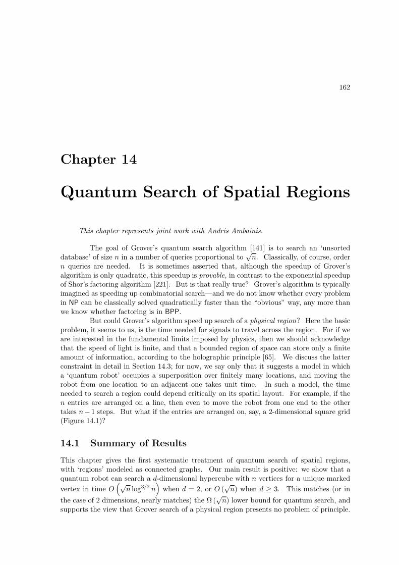
162

Chapter 14

Quantum Search of Spatial Regions

This chapter represents joint work with Andris Ambainis.

The goal of Grover’s quantum search algorithm [141] is to search an ‘unsorteddatabase’ of size n in a number of queries proportional to

√n. Classically, of course, order

n queries are needed. It is sometimes asserted that, although the speedup of Grover’salgorithm is only quadratic, this speedup is provable, in contrast to the exponential speedupof Shor’s factoring algorithm [221]. But is that really true? Grover’s algorithm is typicallyimagined as speeding up combinatorial search—and we do not know whether every problemin NP can be classically solved quadratically faster than the “obvious” way, any more thanwe know whether factoring is in BPP.

But could Grover’s algorithm speed up search of a physical region? Here the basicproblem, it seems to us, is the time needed for signals to travel across the region. For if weare interested in the fundamental limits imposed by physics, then we should acknowledgethat the speed of light is finite, and that a bounded region of space can store only a finiteamount of information, according to the holographic principle [65]. We discuss the latterconstraint in detail in Section 14.3; for now, we say only that it suggests a model in whicha ‘quantum robot’ occupies a superposition over finitely many locations, and moving therobot from one location to an adjacent one takes unit time. In such a model, the timeneeded to search a region could depend critically on its spatial layout. For example, if then entries are arranged on a line, then even to move the robot from one end to the othertakes n− 1 steps. But what if the entries are arranged on, say, a 2-dimensional square grid(Figure 14.1)?

14.1 Summary of Results

This chapter gives the first systematic treatment of quantum search of spatial regions,with ‘regions’ modeled as connected graphs. Our main result is positive: we show that aquantum robot can search a d-dimensional hypercube with n vertices for a unique marked

vertex in time O(√

n log3/2 n)

when d = 2, or O (√n) when d ≥ 3. This matches (or in

the case of 2 dimensions, nearly matches) the Ω (√n) lower bound for quantum search, and

supports the view that Grover search of a physical region presents no problem of principle.

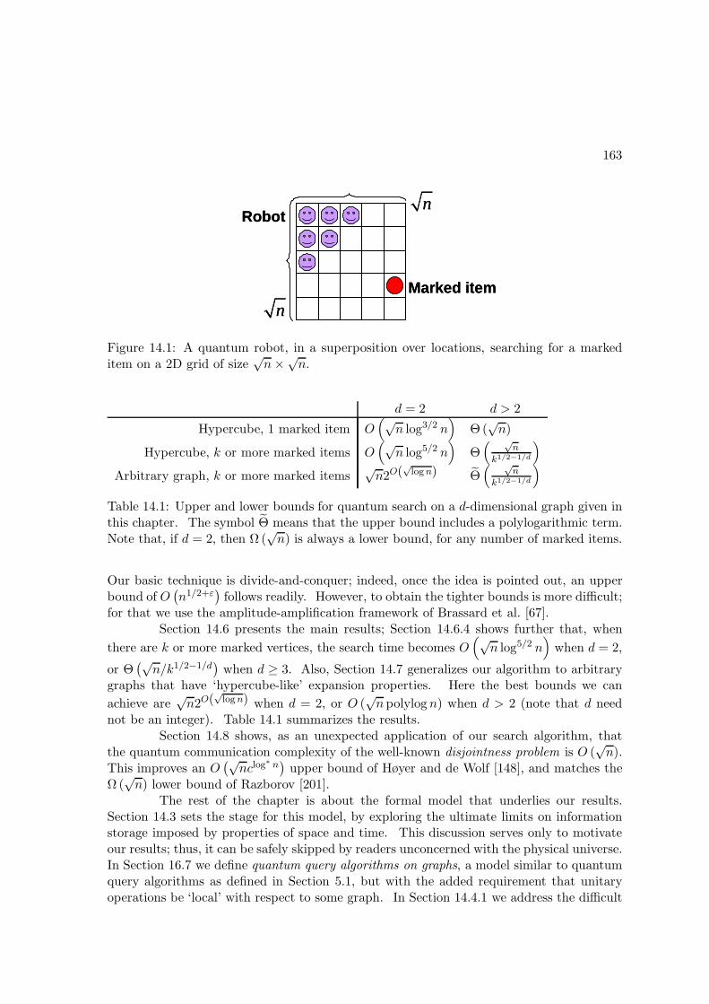
163

Marked item

Robot

n

n

Marked item

Robot

n

n

Figure 14.1: A quantum robot, in a superposition over locations, searching for a markeditem on a 2D grid of size

√n×√

n.

d = 2 d > 2

Hypercube, 1 marked item O(√

n log3/2 n)

Θ (√n)

Hypercube, k or more marked items O(√

n log5/2 n)

Θ( √

n

k1/2−1/d

)

Arbitrary graph, k or more marked items√n2O(

√logn) Θ

( √n

k1/2−1/d

)

Table 14.1: Upper and lower bounds for quantum search on a d-dimensional graph given inthis chapter. The symbol Θ means that the upper bound includes a polylogarithmic term.Note that, if d = 2, then Ω (

√n) is always a lower bound, for any number of marked items.

Our basic technique is divide-and-conquer; indeed, once the idea is pointed out, an upperbound of O

(n1/2+ε

)follows readily. However, to obtain the tighter bounds is more difficult;

for that we use the amplitude-amplification framework of Brassard et al. [67].Section 14.6 presents the main results; Section 14.6.4 shows further that, when

there are k or more marked vertices, the search time becomes O(√

n log5/2 n)

when d = 2,

or Θ(√n/k1/2−1/d

)when d ≥ 3. Also, Section 14.7 generalizes our algorithm to arbitrary

graphs that have ‘hypercube-like’ expansion properties. Here the best bounds we can

achieve are√n2O(

√logn) when d = 2, or O (

√n polylog n) when d > 2 (note that d need

not be an integer). Table 14.1 summarizes the results.Section 14.8 shows, as an unexpected application of our search algorithm, that

the quantum communication complexity of the well-known disjointness problem is O (√n).

This improves an O(√nclog

∗ n)

upper bound of Høyer and de Wolf [148], and matches theΩ (

√n) lower bound of Razborov [201].

The rest of the chapter is about the formal model that underlies our results.Section 14.3 sets the stage for this model, by exploring the ultimate limits on informationstorage imposed by properties of space and time. This discussion serves only to motivateour results; thus, it can be safely skipped by readers unconcerned with the physical universe.In Section 16.7 we define quantum query algorithms on graphs, a model similar to quantumquery algorithms as defined in Section 5.1, but with the added requirement that unitaryoperations be ‘local’ with respect to some graph. In Section 14.4.1 we address the difficult

164

question, which also arises in work on quantum random walks [19] and quantum cellularautomata [238], of what ‘local’ means. Section 14.5 proves general facts about our model,

including an upper bound ofO(√

nδ)

for the time needed to search any graph with diameter

δ, and a proof (using the hybrid argument of Bennett et al. [51]) that this upper bound istight for certain graphs. We conclude in Section 14.9 with some open problems.

14.2 Related Work

In a paper on ‘Space searches with a quantum robot,’ Benioff [50] asked whether Grover’salgorithm can speed up search of a physical region, as opposed to a combinatorial searchspace. His answer was discouraging: for a 2-D grid of size

√n × √

n, Grover’s algorithmis no faster than classical search. The reason is that, during each of the Θ (

√n) Grover

iterations, the algorithm must use order√n steps just to travel across the grid and return

to its starting point for the diffusion step. On the other hand, Benioff noted, Grover’salgorithm does yield some speedup for grids of dimension 3 or higher, since those grids havediameter less than

√n.

Our results show that Benioff’s claim is mistaken: by using Grover’s algorithm

more carefully, one can search a 2-D grid for a single marked vertex in O(√

n log3/2 n)

time. To us this illustrates why one should not assume an algorithm is optimal on heuristicgrounds. Painful experience—for example, the “obviously optimal” O

(n3)

matrix multi-plication algorithm [228]—is what taught computer scientists to see the proving of lowerbounds as more than a formality.

Our setting is related to that of quantum random walks on graphs [19, 83, 84, 218].In an earlier version of this chapter, we asked whether quantum walks might yield analternative spatial search algorithm, possibly even one that outperforms our divide-and-conquer algorithm. Motivated by this question, Childs and Goldstone [86] managed to showthat in the continuous-time setting, a quantum walk can search a d-dimensional hypercubefor a single marked vertex in time O (

√n log n) when d = 4, or O (

√n) when d ≥ 5. Our

algorithm was still faster in 3 or fewer dimensions (see Table 14.2). Subsequently, however,Ambainis, Kempe, and Rivosh [31] gave an algorithm based on a discrete-time quantumwalk, which was as fast as ours in 3 or more dimensions, and faster in 2 dimensions. Inparticular, when d = 2 their algorithm used only O (

√n log n) time to find a unique marked

vertex. Childs and Goldstone [85] then gave a continuous-time quantum walk algorithmwith the same performance, and related this algorithm to properties of the Dirac equation.It is still open whether O (

√n) time is achievable in 2 dimensions.

Currently, the main drawback of the quantum walk approach is that all analyseshave relied heavily on symmetries in the underlying graph. If even minor ‘defects’ areintroduced, it is no longer known how to upper-bound the running time. By contrast,the analysis of our divide-and-conquer algorithm is elementary, and does not depend oneigenvalue bounds. We can therefore show that the algorithm works for any graphs withsufficiently good expansion properties.

Childs and Goldstone [86] argued that the quantum walk approach has the advan-tage of requiring fewer auxiliary qubits than the divide-and-conquer approach. However,

165

d = 2 d = 3 d = 4 d ≥ 5

This chapter O(√

n log3/2 n)

O (√n) O (

√n) O (

√n)

[86] O (n) O(n5/6

)O (

√n log n) O (

√n)

[31, 85] O (√n log n) O (

√n) O (

√n) O (

√n)

Table 14.2: Time needed to find a unique marked item in a d-dimensional hypercube, usingthe divide-and-conquer algorithms of this chapter, the original quantum walk algorithm ofChilds and Goldstone [86], and the improved walk algorithms of Ambainis, Kempe, andRivosh [31] and Childs and Goldstone [85].

the need for many qubits was an artifact of how we implemented the algorithm in a previousversion of the chapter. The current version uses only one qubit.

14.3 The Physics of Databases

Theoretical computer science generally deals with the limit as some resource (such as time ormemory) increases to infinity. What is not always appreciated is that, as the resource boundincreases, physical constraints may come into play that were negligible at ‘sub-asymptotic’scales. We believe theoretical computer scientists ought to know something about suchconstraints, and to account for them when possible. For if the constraints are ignored onthe ground that they “never matter in practice,” then the obvious question arises: why useasymptotic analysis in the first place, rather than restricting attention to those instancesizes that occur in practice?

A constraint of particular interest for us is the holographic principle [65], whicharose from black-hole thermodynamics. The principle states that the information contentof any spatial region is upper-bounded by its surface area (not volume), at a rate of onebit per Planck area, or about 1.4 × 1069 bits per square meter. Intuitively, if one tried tobuild a spherical hard disk with mass density υ, one could not keep expanding it forever.For as soon as the radius reached the Schwarzschild bound of r =

√3/ (8πυ) (in Planck

units, c = G = ~ = k = 1), the hard disk would collapse to form a black hole, and thus itscontents would be irretrievable.

Actually the situation is worse than that: even a planar hard disk of constantmass density would collapse to form a black hole once its radius became sufficiently large,r = Θ (1/υ). (We assume here that the hard disk is disc-shaped. A linear or 1-D harddisk could expand indefinitely without collapse.) It is possible, though, that a hard disk’sinformation content could asymptotically exceed its mass. For example, a black hole’smass is proportional to the radius of its event horizon, but the entropy is proportional tothe square of the radius (that is, to the surface area). Admittedly, inherent difficulties withstorage and retrieval make a black hole horizon less than ideal as a hard disk. However,even a weakly-gravitating system could store information at a rate asymptotically exceedingits mass-energy. For instance, Bousso [65] shows that an enclosed ball of radiation withradius r can store n = Θ

(r3/2

)bits, even though its energy grows only as r. Our results in

Section 14.7.1 will imply that a quantum robot could (in principle!) search such a ‘radiation

166

disk’ for a marked item in time O(r5/4

)= O

(n5/6

). This is some improvement over the

trivial O (n) upper bound for a 1-D hard disk, though it falls short of the desired O (√n).

In general, if n = rc bits are scattered throughout a 3-D ball of radius r (wherec ≤ 3 and the bits’ locations are known), we will show in Theorem 130 that the timeneeded to search for a ‘1’ bit grows as n1/c+1/6 = r1+c/6 (omitting logarithmic factors). Inparticular, if n = Θ

(r2)

(saturating the holographic bound), then the time grows as n2/3 or

r4/3. To achieve a search time of O (√n polylog n), the bits would need to be concentrated

on a 2-D surface.Because of the holographic principle, we see that it is not only quantum mechanics

that yields a Ω (√n) lower bound on the number of steps needed for unordered search. If

the items to be searched are laid out spatially, then general relativity in 3 + 1 dimensionsindependently yields the same bound, Ω (

√n), up to a constant factor.1 Interestingly, in

d+1 dimensions the relativity bound would be Ω(n1/(d−1)

), which for d > 3 is weaker than

the quantum mechanics bound. Given that our two fundamental theories yield the samelower bound, it is natural to ask whether that bound is tight. The answer seems to be thatit is not tight, since (i) the entropy on a black hole horizon is not efficiently accessible2, and(ii) weakly-gravitating systems are subject to the Bekenstein bound [48], an even strongerentropy constraint than the holographic bound.

Yet it is still of basic interest to know whether n bits in a radius-r ball can besearched in time o (min n, r√n)—that is, whether it is possible to do anything betterthan either brute-force quantum search (with the drawback pointed out by Benioff [50]), orclassical search. Our results show that it is possible.

From a physical point of view, several questions naturally arise: (1) whether ourcomplexity measure is realistic; (2) how to account for time dilation; and (3) whether giventhe number of bits we are imagining, cosmological bounds are also relevant. Let us addressthese questions in turn.

(1) One could argue that to maintain a ‘quantum database’ of size n requires ncomputing elements ([251], though see also [208]). So why not just exploit those elementsto search the database in parallel? Then it becomes trivial to show that the search time islimited only by the radius of the database, so the algorithms of this chapter are unnecessary.Our response is that, while there might be n ‘passive’ computing elements (capable of storingdata), there might be many fewer ‘active’ elements, which we consequently wish to place ina superposition over locations. This assumption seems physically unobjectionable. For aparticle (and indeed any object) really does have an indeterminate location, not merely anindeterminate internal state (such as spin) at some location. We leave as an open problem,however, whether our assumption is valid for specific quantum computer architectures suchas ion traps.

(2) So long as we invoke general relativity, should we not also consider the effectsof time dilation? Those effects are indeed pronounced near a black hole horizon. Again,though, for our upper bounds we will have in mind systems far from the Schwarzschild

1Admittedly, the holographic principle is part of quantum gravity and not general relativity per se.All that matters for us, though, is that the principle seems logically independent of quantum-mechanicallinearity, which is what produces the “other” Ω (

√n) bound.

2In the case of a black hole horizon, waiting for the bits to be emitted as Hawking radiation—as recentevidence suggests that they are [211]—takes time proportional to r3, which is much too long.

167

limit, for which any time dilation is by at most a constant factor independent of n.(3) How do cosmological considerations affect our analysis? Bousso [64] argues

that, in a spacetime with positive cosmological constant Λ > 0, the total number of bitsaccessible to any one experiment is at most 3π/ (Λ ln 2), or roughly 10122 given currentexperimental bounds [210] on Λ.3 Intuitively, even if the universe is spatially infinite, mostof it recedes too quickly from any one observer to be harnessed as computer memory.

One response to this result is to assume an idealization in which Λ vanishes,although Planck’s constant ~ does not vanish. As justification, one could argue that withoutthe idealization Λ = 0, all asymptotic bounds in computer science are basically fictions.But perhaps a better response is to accept the 3π/ (Λ ln 2) bound, and then ask how closeone can come to saturating it in different scenarios. Classically, the maximum numberof bits that can be searched is, in a crude model4, actually proportional to 1/

√Λ ≈ 1061

rather than 1/Λ. The reason is that if a region had much more than 1/√

Λ bits, thenafter 1/

√Λ Planck times—that is, about 1010 years, or roughly the current age of the

universe—most of the region would have receded beyond one’s cosmological horizon. Whatour results suggest is that, using a quantum robot, one could come closer to saturating thecosmological bound—since, for example, a 2-D region of size 1/Λ can be searched in time

O(

1√Λ

polylog 1√Λ

). How anyone could prepare (say) a database of size much greater than

1/√

Λ remains unclear, but if such a database existed, it could be searched!

14.4 The Model

As discussed in Part I, much of what is known about the power of quantum computingcomes from the black-box or query model—in which one counts only the number of queriesto an oracle, not the number of computational steps. We will take this model as thestarting point for a formal definition of quantum robots. Doing so will focus attentionon our main concern: how much harder is it to evaluate a function when its inputs arespatially separated? As it turns out, all of our algorithms will be efficient as measured bythe number of gates and auxiliary qubits needed to implement them.

For simplicity, we assume that a robot’s goal is to evaluate a Boolean functionf : 0, 1n → 0, 1, which could be partial or total. A ‘region of space’ is a connectedundirected graph G = (V,E) with vertices V = v1, . . . , vn. Let X = x1 . . . xn ∈ 0, 1nbe an input to f ; then each bit xi is available only at vertex vi. We assume the robotknows G and the vertex labels in advance, and so is ignorant only of the xi bits. We thussidestep a major difficulty for quantum walks [19], which is how to ensure that a processon an unknown graph is unitary.

3Also, Lloyd [172] argues that the total number of bits accessible up till now is at most the square of the

number of Planck times elapsed so far, or about(1061

)2= 10122. Lloyd’s bound, unlike Bousso’s, does not

depend on Λ being positive. The numerical coincidence between the two bounds reflects the experimentalfinding [210, 209] that we live in a transitional era, when both Λ and “dust” contribute significantly to theuniverse’s net energy balance (ΩΛ ≈ 0.7, Ωdust ≈ 0.3). In earlier times dust (and before that radiation)dominated, and Lloyd’s bound was tighter. In later times Λ will dominate, and Bousso’s bound will betighter. Why we should live in such a transitional era is unknown.

4Specifically, neglecting gravity and other forces that could counteract the effect of Λ.

168

At any time, the robot’s state has the form

∑αi,z |vi, z〉 .

Here vi ∈ V is a vertex, representing the robot’s location; and z is a bit string (which canbe arbitrarily long), representing the robot’s internal configuration. The state evolves viaan alternating sequence of T algorithm steps and T oracle steps:

U (1) → O(1) → U (1) → · · · → U (T ) → O(T ).

An oracle step O(t) maps each basis state |vi, z〉 to |vi, z ⊕ xi〉, where xi is exclusive-OR’edinto the first bit of z. An algorithm step U (t) can be any unitary matrix that (1) does notdepend on X, and (2) acts ‘locally’ on G. How to make the second condition precise is thesubject of Section 14.4.1.

The initial state of the algorithm is |v1, 0〉. Let α(t)i,z (X) be the amplitude of |vi, z〉

immediately after the tth oracle step; then the algorithm succeeds with probability 1 − ε if

∑

|vi,z〉 : zOUT =f(X)

∣∣∣α(T )i,z (X)

∣∣∣2≥ 1 − ε

for all inputs X, where zOUT is a bit of z representing the output.

14.4.1 Locality Criteria

Classically, it is easy to decide whether a stochastic matrix acts locally with respect to agraph G: it does if it moves probability only along the edges of G. In the quantum case,however, interference makes the question much more subtle. In this section we proposethree criteria for whether a unitary matrix U is local. Our algorithms can be implementedusing the most restrictive of these criteria, whereas our lower bounds apply to all three ofthem.

The first criterion we call Z-locality (for zero): U is Z-local if, given any pair ofnon-neighboring vertices v1, v2 in G, U “sends no amplitude” from v1 to v2; that is, thecorresponding entries in U are all 0. The second criterion, C-locality (for composability),says that this is not enough: not only must U send amplitude only between neighboringvertices, but it must be composed of a product of commuting unitaries, each of which actson a single edge. The third criterion is perhaps the most natural one to a physicist: Uis H-local (for Hamiltonian) if it can be obtained by applying a locally-acting, low-energyHamiltonian for some fixed amount of time. More formally, let Ui,z→i∗,z∗ be the entry inthe |vi, z〉 column and |vi∗ , z∗〉 row of U .

Definition 101 U is Z-local if Ui,z→i∗,z∗ = 0 whenever i 6= i∗ and (vi, vi∗) is not an edgeof G.

Definition 102 U is C-local if the basis states can be partitioned into subsets P1, . . . , Pqsuch that

(i) Ui,z→i∗,z∗ = 0 whenever |vi, z〉 and |vi∗ , z∗〉 belong to distinct Pj ’s, and

169

(ii) for each j, all basis states in Pj are either from the same vertex or from two adjacentvertices.

Definition 103 U is H-local if U = eiH for some Hermitian H with eigenvalues of absolutevalue at most π, such that Hi,z→i∗,z∗ = 0 whenever i 6= i∗ and (vi, vi∗) is not an edge in E.

If a unitary matrix is C-local, then it is also Z-local and H-local. For the latterimplication, note that any unitary U can be written as eiH for some H with eigenvalues ofabsolute value at most π. So we can write the unitary Uj acting on each Pj as eiHj ; thensince the Uj ’s commute, ∏

Uj = ei∑Hj .

Beyond that, though, how are the locality criteria related? Are they approximately equiva-lent? If not, then does a problem’s complexity in our model ever depend on which criterionis chosen? Let us emphasize that these questions are not answered by, for example, theSolovay-Kitaev theorem (see [184]), that an n×n unitary matrix can be approximated usinga number of gates polynomial in n. For recall that the definition of C-locality requires theedgewise operations to commute—indeed, without that requirement, one could produce anyunitary matrix at all. So the relevant question, which we leave open, is whether any Z-localor H-local unitary can be approximated by a product of, say, O (log n) C-local unitaries.(A product of O (n) such unitaries trivially suffices, but that is far too many.) Again, thealgorithms in this chapter will use C-local unitaries, whereas the lower bounds will applyeven to Z-local and H-local unitaries.

14.5 General Bounds

Given a Boolean function f : 0, 1n → 0, 1, the quantum query complexity Q (f) isthe minimum T for which there exists a T -query quantum algorithm that evaluates fwith probability at least 2/3 on all inputs. (We will always be interested in the two-sided,bounded-error complexity, denoted Q2 (f) elsewhere in this thesis.) Similarly, given a graphG with n vertices labeled 1, . . . , n, we let Q (f,G) be the minimum T for which there existsa T -query quantum robot on G that evaluates f with probability 2/3. Here the algorithmsteps must be C-local; we use QZ (f,G) and QH (f,G) to denote the corresponding measurewith Z-local and H-local steps respectively. Clearly Q (f,G) ≥ QZ (f,G) and Q (f,G) ≥QH (f,G); we do not know whether all three measures are asymptotically equivalent.

Let δG be the diameter of G, and call f nondegenerate if it depends on all n inputbits.

Proposition 104 For all f,G,

(i) Q (f,G) ≤ 2n − 3.

(ii) Q (f,G) ≤ (2δG + 1)Q (f).

(iii) Q (f,G) ≥ Q (f).

(iv) Q (f,G) ≥ δG/2 if f is nondegenerate.

170

Proof.

(i) Starting from the root, a spanning tree for G can be traversed in 2 (n− 1) − 1 steps(there is no need to return to the root).

(ii) We can simulate a query in 2δG steps, by fanning out from the start vertex v1 andthen returning. Applying a unitary at v1 takes 1 step.

(iii) Obvious.

(iv) There exists a vertex vi whose distance to v1 is at least δG/2, and f could depend onxi.

We now show that the model is robust.

Proposition 105 For nondegenerate f , the following change Q (f,G) by at most a constantfactor.

(i) Replacing the initial state |v1, 0〉 by an arbitrary (known) |ψ〉.

(ii) Requiring the final state to be localized at some vertex vi with probability at least 1−ε,for a constant ε > 0.

(iii) Allowing multiple algorithm steps between each oracle step (and measuring the com-plexity by the number of algorithm steps).

Proof.

(i) We can transform |v1, 0〉 to |ψ〉 (and hence |ψ〉 to |v1, 0〉) in δG = O (Q (f,G)) steps,by fanning out from v1 along the edges of a minimum-height spanning tree.

(ii) Assume without loss of generality that zOUT is accessed only once, to write the output.Then after zOUT is accessed, uncompute (that is, run the algorithm backwards) tolocalize the final state at v1. The state can then be localized at any vi in δG =O (Q (f,G)) steps. We can succeed with any constant probability by repeating thisprocedure a constant number of times.

(iii) The oracle step O is its own inverse, so we can implement a sequence U1, U2, . . . ofalgorithm steps as follows (where I is the identity):

U1 → O → I → O → U2 → · · ·

A function of particular interest is f = OR(x1, . . . , xn), which outputs 1 if andonly if xi = 1 for some i. We first give a general upper bound on Q (OR, G) in terms ofthe diameter of G. (Throughout the chapter, we sometimes omit floor and ceiling signs ifthey clearly have no effect on the asymptotics.)

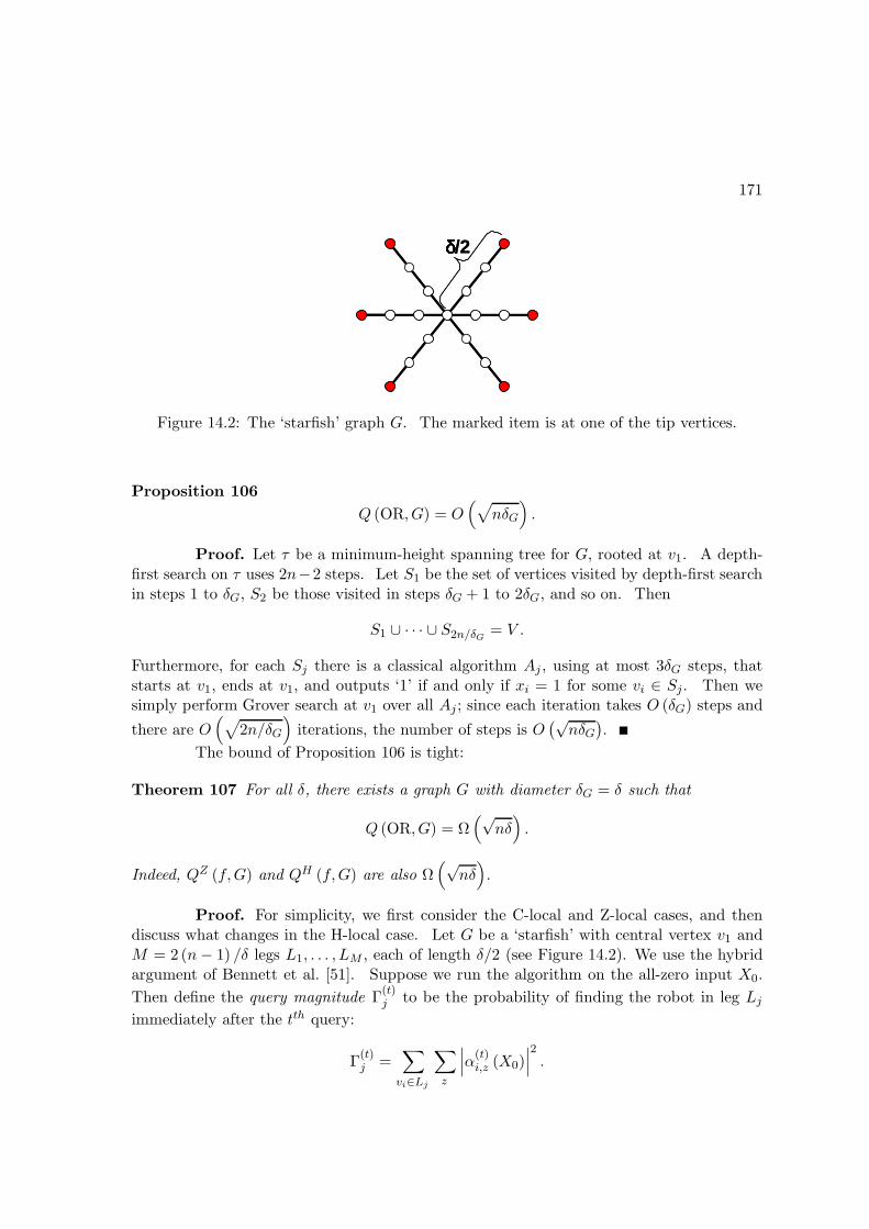
171

δδδδ/2δδδδ/2

Figure 14.2: The ‘starfish’ graph G. The marked item is at one of the tip vertices.

Proposition 106

Q (OR, G) = O(√

nδG

).

Proof. Let τ be a minimum-height spanning tree for G, rooted at v1. A depth-first search on τ uses 2n−2 steps. Let S1 be the set of vertices visited by depth-first searchin steps 1 to δG, S2 be those visited in steps δG + 1 to 2δG, and so on. Then

S1 ∪ · · · ∪ S2n/δG = V .

Furthermore, for each Sj there is a classical algorithm Aj , using at most 3δG steps, thatstarts at v1, ends at v1, and outputs ‘1’ if and only if xi = 1 for some vi ∈ Sj. Then wesimply perform Grover search at v1 over all Aj ; since each iteration takes O (δG) steps and

there are O(√

2n/δG

)iterations, the number of steps is O

(√nδG

).

The bound of Proposition 106 is tight:

Theorem 107 For all δ, there exists a graph G with diameter δG = δ such that

Q (OR, G) = Ω(√

nδ).

Indeed, QZ (f,G) and QH (f,G) are also Ω(√

nδ).

Proof. For simplicity, we first consider the C-local and Z-local cases, and thendiscuss what changes in the H-local case. Let G be a ‘starfish’ with central vertex v1 andM = 2 (n− 1) /δ legs L1, . . . , LM , each of length δ/2 (see Figure 14.2). We use the hybridargument of Bennett et al. [51]. Suppose we run the algorithm on the all-zero input X0.

Then define the query magnitude Γ(t)j to be the probability of finding the robot in leg Lj

immediately after the tth query:

Γ(t)j =

∑

vi∈Lj

∑

z

∣∣∣α(t)i,z (X0)

∣∣∣2.

172

Let T be the total number of queries, and let w = T/ (cδ) for some constant 0 < c < 1/2.Clearly

w−1∑

q=0

M∑

j=1

Γ(T−qcδ)j ≤

w−1∑

q=0

1 = w.

Hence there must exist a leg Lj∗ such that

w−1∑

q=0

Γ(T−qcδ)j∗ ≤ w

M=

wδ

2 (n− 1).

Let vi∗ be the tip vertex of Lj∗, and let Y be the input which is 1 at vi∗ and 0 elsewhere.Then let Xq be a hybrid input, which is X0 during queries 1 to T − qcδ, but Y duringqueries T − qcδ + 1 to T . Also, let

∣∣∣ψ(t) (Xq)⟩

=∑

i,z

α(t)i,z (Xq) |vi, z〉

be the algorithm’s state after t queries when run on Xq, and let

D (q, r) =∥∥∥∣∣∣ψ(T ) (Xq)

⟩−∣∣∣ψ(T ) (Xr)

⟩∥∥∥2

2

=∑

vi∈G

∑

z

∣∣∣α(T )i,z (Xq) − α

(T )i,z (Xr)

∣∣∣2.

Then for all q ≥ 1, we claim that D (q − 1, q) ≤ 4Γ(T−qcδ)j∗ . For by unitarity, the Euclidean

distance between∣∣ψ(t) (Xq−1)

⟩and

∣∣ψ(t) (Xq)⟩

can only increase as a result of queries T −qcδ + 1 through T − (q − 1) cδ. But no amplitude from outside Lj∗ can reach vi∗ duringthat interval, since the distance is δ/2 and there are only cδ < δ/2 time steps. Therefore,switching from Xq−1 to Xq can only affect amplitude that is in Lj∗ immediately after queryT − qcδ:

D (q − 1, q) ≤∑

vi∈Lj∗

∑

z

∣∣∣α(T−qcδ)i,z (Xq) −

(−α(T−qcδ)

i,z (Xq))∣∣∣

2

= 4∑

vi∈Lj∗

∑

z

∣∣∣α(T−qcδ)i,z (X0)

∣∣∣2

= 4Γ(T−qcδ)j∗ .

It follows that

√D (0, w) ≤

w∑

q=1

√D (q − 1, q) ≤ 2

w∑

q=1

√Γ

(T−qcδ)j∗ ≤ 2w

√δ

2 (n− 1)=T

c

√2

δ (n− 1).

Here the first inequality uses the triangle inequality, and the third uses the Cauchy-Schwarzinequality. Now assuming the algorithm is correct we need D (0, w) = Ω (1), which implies

that T = Ω(√

nδ).

173

In the H-local case, it is no longer true that no amplitude from outside Lj∗ canreach vi∗ in cδ time steps. But if c is a small enough constant, then the amount ofamplitude that can reach vi∗ decreases exponentially in δ. To see this, assume withoutloss of generality that all amplitude not in Lj∗ starts in the state |v0, ψ〉, where |ψ〉 is somesuperposition over auxiliary qubits. Let H be the local Hamiltonian that acts between thetth and (t+ 1)st queries, all of whose eigenvalues have absolute value at most π. Since His Hermitian, we can decompose it as V ΛV −1 where V is unitary and Λ is diagonal. So byTaylor series expansion,

eiH =∑

j≥0

ij

j!V ΛjV −1.

Now let S be the set of basis states |vb, zb〉 such that the distance from v0 to vb is `, forsome ` > 4π. Notice that for all j < ` and |vb, zb〉 ∈ S, we have

〈vb, zb|Hj |v0, ψ〉 = 〈vb, zb|V ΛjV −1 |v0, ψ〉 = 0

by the locality of H. Therefore

∑

|vb,zb〉∈S

∣∣〈vb, zb| eiH |v0, ψ〉∣∣2 =

∑

|vb,zb〉∈S

∣∣∣∣∣∣

∑

j≥`

ij

j!〈vb, zb|V ΛjV −1 |v0, ψ〉

∣∣∣∣∣∣

2

≤

∑

j≥`

√√√√∑

|vb,zb〉∈S

∣∣∣∣ij

j!〈vb, zb|V ΛjV −1 |v0, ψ〉

∣∣∣∣2

2

≤

∑

j≥`

√πj

j!

2

≤ 4π`

`!.

Here the second line uses the triangle inequality, the third line uses the fact that V ΛjV −1 hasmaximum eigenvalue at most πj (and therefore

(ij/j!

)V ΛjV −1 has maximum eigenvalue at

most πj/j!), and the fourth line uses the fact that ` > 4π. Intuitively, the probability thatH sends the robot a distance ` from v0 is at most 4π`/`!, which decreases exponentially in`. One can now use a Chernoff-Hoeffding bound to upper-bound the probability that cδlocal Hamiltonians, applied in succession, ever move the robot a distance δ/2 from v0. Itis clear that the resulting upper bound is 2−Ω(δ) for small enough c. Therefore

D (q − 1, q) ≤ 4Γ(T−qcδ)j∗ + 2−Ω(δ)

and the remainder of the proof goes through as before.

14.6 Search on Grids

Let Ld (n) be a d-dimensional grid graph of size n1/d × · · · × n1/d. That is, each vertexis specified by d coordinates i1, . . . , id ∈

1, . . . , n1/d

, and is connected to the at most 2d

174

vertices obtainable by adding or subtracting 1 from a single coordinate (boundary verticeshave fewer than 2d neighbors). We write simply Ld when n is clear from context. Inthis section we present our main positive results: that Q (OR,Ld) = Θ (

√n) for d ≥ 3, and

Q (OR,L2) = O (√n polylog n) for d = 2.

Before proving these claims, let us develop some intuition by showing weakerbounds, taking the case d = 2 for illustration. Clearly Q (OR,L2) = O

(n3/4

): we simply

partition L2 (n) into√n subsquares, each a copy of L2 (

√n). In 5

√n steps, the robot can

travel from the start vertex to any subsquare C, search C classically for a marked vertex,and then return to the start vertex. Thus, by searching all

√n of the C’s in superposition

and applying Grover’s algorithm, the robot can search the grid in time O(n1/4

)× 5

√n =

O(n3/4

).

Once we know that, we might as well partition L2 (n) into n1/3 subsquares, each acopy of L2

(n2/3

). Searching any one of these subsquares by the previous algorithm takes

time O((n2/3

)3/4)= O (

√n), an amount of time that also suffices to travel to the subsquare

and back from the start vertex. So using Grover’s algorithm, the robot can search L2 (n) in

time O(√

n1/3 · √n)

= O(n2/3

). We can continue recursively in this manner to make the

running time approach O (√n). The trouble is that, with each additional layer of recursion,

the robot needs to repeat the search more often to upper-bound the error probability. Usingthis approach, the best bounds we could obtain are roughly O (

√npolylog n) for d ≥ 3, or√

n2O(√

logn) for d = 2. In what follows, we use the amplitude amplification approachof Brassard et al. [67] to improve these bounds, in the case of a single marked vertex, to

O (√n) for d ≥ 3 (Section 14.6.2) and O

(√n log3/2 n

)for d = 2 (Section 14.6.3). Section

14.6.4 generalizes these results to the case of multiple marked vertices.Intuitively, the reason the case d = 2 is special is that there, the diameter of the

grid is Θ (√n), which matches exactly the time needed for Grover search. For d ≥ 3, by

contrast, the robot can travel across the grid in much less time than is needed to search it.

14.6.1 Amplitude Amplification

We start by describing amplitude amplification [67], a generalization of Grover search. LetA be a quantum algorithm that, with probability ε, outputs a correct answer together witha witness that proves the answer correct. (For example, in the case of search, the algorithmoutputs a vertex label i such that xi = 1.) Amplification generates a new algorithm thatcalls A order 1/

√ε times, and that produces both a correct answer and a witness with

probability Ω (1). In particular, assume A starts in basis state |s〉, and let m be a positiveinteger. Then the amplification procedure works as follows:

(1) Set |ψ0〉 = A |s〉.

(2) For i = 1 to m set |ψi+1〉 = ASA−1W |ψi〉, where

• W flips the phase of basis state |y〉 if and only if |y〉 contains a description of acorrect witness, and

• S flips the phase of basis state |y〉 if and only if |y〉 = |s〉.

175

We can decompose |ψ0〉 as sinα |Ψsucc〉 + cosα |Ψfail〉, where |Ψsucc〉 is a superpo-sition over basis states containing a correct witness and |Ψfail〉 is a superposition over allother basis states. Brassard et al. [67] showed the following:

Lemma 108 ([67]) |ψi〉 = sin [(2i+ 1)α] |Ψsucc〉 + cos [(2i+ 1)α] |Ψfail〉.

If measuring |ψ0〉 gives a correct witness with probability ε, then |sinα|2 = ε and|α| ≥ 1/

√ε. So taking m = O(1/

√ε) yields sin [(2m+ 1)α] ≈ 1. For our algorithms,

though, the multiplicative constant under the big-O also matters. To upper-bound thisconstant, we prove the following lemma.

Lemma 109 Suppose a quantum algorithm A outputs a correct answer and witness withprobability exactly ε. Then by using 2m+ 1 calls to A or A−1, where

m ≤ π

4 arcsin√ε− 1

2,

we can output a correct answer and witness with probability at least

(1 − (2m+ 1)2

3ε

)(2m+ 1)2 ε.

Proof. We perform m steps of amplitude amplification, which requires 2m + 1calls A or A−1. By Lemma 108, this yields the final state

sin [(2m+ 1)α] |Ψsucc〉 + cos [(2m+ 1)α] |Ψfail〉 .

where α = arcsin√ε. Therefore the success probability is

sin2[(2m+ 1) arcsin

√ε]≥ sin2

[(2m+ 1)

√ε]

≥(

(2m+ 1)√ε− (2m+ 1)3

6ε3/2

)2

≥ (2m+ 1)2 ε− (2m+ 1)4

3ε2.

Here the first line uses the monotonicity of sin2 x in the interval [0, π/2], and the secondline uses the fact that sinx ≥ x− x3/6 for all x ≥ 0 by Taylor series expansion.

Note that there is no need to uncompute any garbage left by A, beyond theuncomputation that happens “automatically” within the amplification procedure.

14.6.2 Dimension At Least 3

Our goal is the following:

Theorem 110 If d ≥ 3, then Q (OR,Ld) = Θ (√n).

176

In this section, we prove Theorem 110 for the special case of a unique markedvertex; then, in Sections 14.6.4 and 14.6.5, we will generalize to multiple marked vertices.Let OR(k) be the problem of deciding whether there are no marked vertices or exactly k ofthem, given that one of these is true. Then:

Theorem 111 If d ≥ 3, then Q(OR(1),Ld

)= Θ (

√n).

Choose constants β ∈ (2/3, 1) and µ ∈ (1/3, 1/2) such that βµ > 1/3 (for example,β = 4/5 and µ = 5/11 will work). Let `0 be a large positive integer; then for all positive

integers R, let `R = `R−1

⌈`1/β−1R−1

⌉. Also let nR = `dR. Assume for simplicity that n = nR

for some R; in other words, that the hypercube Ld (nR) to be searched has sides of length`R. Later we will remove this assumption.

Consider the following recursive algorithm A. If n = n0, then search Ld (n0)classically, returning 1 if a marked vertex is found and 0 otherwise. Otherwise partitionLd (nR) into nR/nR−1 subcubes, each one a copy of Ld (nR−1). Take the algorithm thatconsists of picking a subcube C uniformly at random, and then running A recursively onC. Amplify this algorithm (nR/nR−1)

µ times.

The intuition behind the exponents is that nR−1 ≈ nβR, so searching Ld (nR−1)

should take about nβ/2R steps, which dominates the n

1/dR steps needed to travel across the

hypercube when d ≥ 3. Also, at level R we want to amplify a number of times thatis less than (nR/nR−1)

1/2 by some polynomial amount, since full amplification would beinefficient. The reason for the constraint βµ > 1/3 will appear in the analysis.

We now provide a more explicit description of A, which shows that A can beimplemented using C-local unitaries and only a single bit of workspace. At any time, thequantum robot’s state will have the form

∑i,z αi,z |vi, z〉, where vi is a vertex of Ld (nR)

and z is a single bit that records whether or not a marked vertex has been found. Given asubcube C, let v (C) be the “corner” vertex of C; that is, the vertex that is minimal in all dcoordinates. Then the initial state when searching C will be |v (C) , 0〉. Beware, however,that “initial state” in this context just means the state |s〉 from Section 14.6.1. Becauseof the way amplitude amplification works, A will often be invoked on C with other initialstates, and even run in reverse.

Below we give pseudocode for A. Our procedure calls the three unitaries A, W ,and S from Section 14.6.1 as subroutines. For convenience, we write AR, AR,WR, SR todenote the level of recursion that is currently active.

Algorithm 112 (AR) Searches a subcube C of size nR for the marked vertex, and amplifiesthe result to have larger probability. Default initial state: |v (C) , 0〉.

If R = 0 then:

(1) Use classical C-local operations to visit all n0 vertices of C in any order. At eachvi ∈ C, use a query transformation to map the state |vi, z〉 to |vi, z ⊕ xi〉.

(2) Return to v (C).

If R ≥ 1 then:

177

(1) Let mR be the smallest integer such that 2mR + 1 ≥ (nR/nR−1)µ.

(2) Call AR.

(3) For i = 1 to mR, call WR, then A−1R , then SR, then AR.

Suppose AR is run on the initial state |v (C) , 0〉, and let C1, . . . , CnR/n0be the

minimal subcubes in C—meaning those of size n0. Then the final state after AR terminatesshould be

1√nR/n0

nR/n0∑

i=1

|v (Ci) , 0〉

if C does not contain the marked vertex. Otherwise the final state should have non-negligible overlap with |v (Ci∗) , 1〉, where Ci∗ is the minimal subcube in C that containsthe marked vertex. In particular, if R = 0, then the final state should be |v (C) , 1〉 if Ccontains the marked vertex, and |v (C) , 0〉 otherwise.

The two phase-flip subroutines, WR and SR, are both trivial to implement. Toapply WR, map each basis state |vi, z〉 to (−1)z |vi, z〉. To apply SR, map each basis state|vi, z〉 to − |vi, z〉 if vi = v (C) for some subcube C of size nR, and to |vi, z〉 otherwise.Below we give pseudocode for AR.

Algorithm 113 (AR) Searches a subcube C of size nR for the marked vertex. Defaultinitial state: |v (C) , 0〉.(1) Partition C into nR/nR−1 smaller subcubes C1, . . . , CnR/nR−1

, each of size nR−1.

(2) For all j ∈ 1, . . . , d, let Vj be the set of corner vertices v (Ci) that differ from v (C)

only in the first j coordinates. Thus V0 = v (C), and in general |Vj | = `jR. Forj = 1 to d, let |Vj〉 be the state

|Vj〉 =1

`j/2R

∑

v(Ci)∈Vj

|v (Ci) , 0〉

Apply a sequence of transformations U1, U2, . . ., Ud where Uj is a unitary that maps|Vj−1〉 to |Vj〉 by applying C-local unitaries that move amplitude only along the jth

coordinate.

(3) Call AR−1 recursively, to search C1, . . . , CnR/nR−1in superposition and amplify the

results.

If AR is run on the initial state |v (C) , 0〉, then the final state should be

1√nR/nR−1

nR/n0∑

i=1

|φi〉 ,

where |φi〉 is the correct final state when AR−1 is run on subcube Ci with initial state|v (Ci) , 0〉. A key point is that there is no need for AR to call AR−1 twice, once to computeand once to uncompute—for the uncomputation is already built in to A. This is what willenable us to prove an upper bound of O (

√n) instead of O

(√n2R

)= O (

√n polylog n).

We now analyze the running time of A.

178

Lemma 114 AR uses O(nµR)

steps.

Proof. Let TA (R) and TA (R) be the total numbers of steps used by AR and ARrespectively in searching Ld (nR). Then we have TA (0) = O (1), and

TA (R) ≤ (2mR + 1)TA (R) + 2mR,

TA (R) ≤ dn1/dR + TA (R− 1)

for all R ≥ 1. For WR and SR can both be implemented in a single step, while AR uses

d`R = dn1/dR steps to move the robot across the hypercube. Combining,

TA (R) ≤ (2mR + 1)(dn

1/dR + TA (R− 1)

)+ 2mR

≤ ((nR/nR−1)µ + 2)

(dn

1/dR + TA (R− 1)

)+ (nR/nR−1)

µ + 1

= O((nR/nR−1)

µ n1/dR

)+ ((nR/nR−1)

µ + 2)TA (R− 1)

= O((nR/nR−1)

µ n1/dR

)+ (nR/nR−1)

µ TA (R− 1)

= O((nR/nR−1)

µ n1/dR + (nR/nR−2)

µ n1/dR−1 + · · · + (nR/n0)

µ n1/d1

)

= nµR ·O(n

1/dR

nµR−1

+n

1/dR−1

nµR−2

+ · · · + n1/d1

nµ0

)

= nµR ·O(n

1/d−βµR + · · · + n

1/d−βµ2 + n

1/d−βµ1

)

= nµR ·O(n

1/d−βµR +

(n

1/d−βµR

)1/β+ · · · +

(n

1/d−βµR

)1/βR−1)

= O(nµR).

Here the second line follows because 2mR + 1 ≤ (nR/nR−1)µ + 2, the fourth because the

(nR/nR−1)µ terms increase doubly exponentially, so adding 2 to each will not affect the

asymptotics; the seventh because nµi = Ω((nµi+1

)β), the eighth because nR−1 ≤ nβR; and

the last because βµ > 1/3 ≥ 1/d, hence n1/d−βµ1 < 1.

Next we need to lower-bound the success probability. Say that A or A “succeeds”if a measurement in the standard basis yields the result |v (Ci∗) , 1〉, where Ci∗ is the minimalsubcube that contains the marked vertex. Of course, the marked vertex itself can then befound in n0 = O (1) steps.

Lemma 115 Assuming there is a unique marked vertex, AR succeeds with probability Ω(1/n1−2µ

R

).

Proof. Let PA (R) and PA (R) be the success probabilities of AR and AR respec-tively when searching Ld (nR). Then clearly PA (0) = 1, and PA (R) = (nR−1/nR)PA (R− 1)

179

for all R ≥ 1. So by Lemma 109,

PA (R) ≥(

1 − 1

3(2mR + 1)2 PA (R)

)(2mR + 1)2 PA (R)

=

(1 − 1

3(2mR + 1)2

nR−1

nRPA (R− 1)

)(2mR + 1)2

nR−1

nRPA (R− 1)

≥(

1 − 1

3(nR/nR−1)

2µ nR−1

nRPA (R− 1)

)(nR/nR−1)

2µ nR−1

nRPA (R− 1)

≥(

1 − 1

3(nR−1/nR)1−2µ

)(nR−1/nR)1−2µ PA (R− 1)

≥ (n0/nR)1−2µR∏

r=1

(1 − 1

3(nR−1/nR)1−2µ

)

≥ (n0/nR)1−2µR∏

r=1

(1 − 1

3n(1−β)(1−2µ)R

)

≥ (n0/nR)1−2µ

(1 −

R∑

r=1

1

3N(1−β)(1−2µ)R

)

= Ω(1/n1−2µ

R

).

Here the third line follows because 2mR + 1 ≥ nR−1/nR and the function x − 13x

2 isnondecreasing in the interval [0, 1]; the fourth because PA (R− 1) ≤ 1; the sixth because

nR−1 ≤ nβR; and the last because β < 1 and µ < 1/2, the nR’s increase doubly exponentially,and n0 is sufficiently large.

Finally, take AR itself and amplify it to success probability Ω (1) by running it

O(n1/2−µR ) times. This yields an algorithm for searching Ld (nR) with overall running time

O(n

1/2R

), which implies that Q

(OR(1),Ld (nR)

)= O

(n

1/2R

).

All that remains is to handle values of n that do not equal nR for any R. The so-

lution is simple: first find the largest R such that nR < n. Then set n′ = nR⌈n1/d/`R

⌉d, and

embed Ld (n) into the larger hypercubeLd (n′). ClearlyQ(OR(1),Ld (n)

)≤ Q

(OR(1),Ld (n′)

).

Also notice that n′ = O (n) and that n′ = O(n

1/βR

)= O

(n

3/2R

). Next partition Ld (n′)

into n′/nR subcubes, each a copy of Ld (nR). The algorithm will now have one additionallevel of recursion, which chooses a subcube of Ld (n′) uniformly at random, runs AR on

that subcube, and then amplifies the resulting procedure Θ(√

n′/nR)

times. The total

time is now

O

(√n′

nR

((n′)1/d

+ n1/2R

))= O

(√n′

nRn

1/2R

)= O

(√n),

while the success probability is Ω (1). This completes Theorem 111.

180

14.6.3 Dimension 2

In the d = 2 case, the best we can achieve is the following:

Theorem 116 Q (OR,L2) = O(√

n log5/2 n).

Again, we start with the single marked vertex case and postpone the general caseto Sections 14.6.4 and 14.6.5.

Theorem 117 Q(OR(1),L2

)= O

(√n log3/2 n

).

For d ≥ 3, we performed amplification on large (greater than O(1/n1−2µ

)) proba-

bilities only once, at the end. For d = 2, on the other hand, any algorithm that we constructwith any nonzero success probability will have running time Ω (

√n), simply because that

is the diameter of the grid. If we want to keep the running time O (√n), then we can

only perform O (1) amplification steps at the end. Therefore we need to keep the successprobability relatively high throughout the recursion, meaning that we suffer an increase inthe running time, since amplification to high probabilities is less efficient.

The procedures AR, AR, WR, and SR are identical to those in Section 14.6.2; allthat changes are the parameter settings. For all integers R ≥ 0, we now let nR = `2R0 , forsome odd integer `0 ≥ 3 to be set later. Thus, AR and AR search the square grid L2 (nR) ofsize `R0 × `R0 . Also, let m = (`0 − 1) /2; then AR applies m steps of amplitude amplificationto AR.

We now prove the counterparts of Lemmas 114 and 115 for the two-dimensionalcase.

Lemma 118 AR uses O(R`R+1

0

)steps.

Proof. Let TA (R) and TA (R) be the time used by AR and AR respectively insearching L2 (nR). Then TA (0) = 1, and for all R ≥ 1,

TA (R) ≤ (2m+ 1)TA (R) + 2m,

TA (R) ≤ 2n1/2R + TA (R− 1) .

Combining,

TA (R) ≤ (2m+ 1)(2n

1/2R + TA (R− 1)

)+ 2m

= `0(2`R0 + TA (R− 1)

)+ `0 − 1

= O(`R+10 + `0TA (R− 1)

)

= O(R`R+1

0

).

Lemma 119 AR succeeds with probability Ω (1/R).

181

Proof. Let PA (R) and PA (R) be the success probabilities of AR and AR respec-tively when searching L2 (nR). Then PA (R) = PA (R− 1) /`20 for all R ≥ 1. So by Lemma109, and using the fact that 2m+ 1 = `0,

PA (R) ≥(

1 − (2m+ 1)2

3PA (R)

)(2m+ 1)2 PA (R)

=

(1 − `20

3

PA (R− 1)

`20

)`20PA (R− 1)

`20

= PA (R− 1) − 1

3P 2A (R− 1)

= Ω (1/R) .

This is because Ω (R) iterations of the map xR := xR−1 − 13x

2R−1 are needed to drop from

(say) 2/R to 1/R, and x0 = PA (0) = 1 is greater than 2/R.

We can amplify AR to success probability Ω (1) by repeating it O(√

R)

times.

This yields an algorithm for searching L2 (nR) that uses O(R3/2`R+1

0

)= O

(√nRR

3/2`0)

steps in total. We can minimize this expression subject to `2R0 = nR by taking `0 to be

constant and R to be Θ (log nR), which yields Q(OR(1),L2 (nR)

)= O

(√nR log n

3/2R

). If

n is not of the form `2R0 , then we simply find the smallest integer R such that n < `2R0 , andembed L2 (n) in the larger grid L2

(`2R0). Since `0 is a constant, this increases the running

time by at most a constant factor. We have now proved Theorem 117.

14.6.4 Multiple Marked Items

What about the case in which there are multiple i’s with xi = 1? If there are k markeditems (where k need not be known in advance), then Grover’s algorithm can find a marked

item with high probability in O(√

n/k)

queries, as shown by Boyer et al. [66]. In our

setting, however, this is too much to hope for—since even if there are many marked vertices,they might all be in a faraway part of the hypercube. Then Ω

(n1/d

)steps are needed,

even if√n/k < n1/d. Indeed, we can show a stronger lower bound. Recall that OR(k) is

the problem of deciding whether there are no marked vertices or exactly k of them.

Theorem 120 For all constants d ≥ 2,

Q(OR(k),Ld

)= Ω

( √n

k1/2−1/d

).

Proof. For simplicity, we assume that both k1/d and(n/3dk

)1/dare integers. (In

the general case, we can just replace k by⌈k1/d

⌉dand n by the largest number of the form

(3m⌈k1/d

⌉)dwhich is less than n. This only changes the lower bound by a lower order

term.)We use a hybrid argument almost identical to that of Theorem 107. Divide Ld

into n/k subcubes, each having k vertices and side length k1/d. Let S be a regularly-spaced

182

set of M = n/(3dk)

of these subcubes, so that any two subcubes in S have distance at least

2k1/d from one another. Then choose a subcube Cj ∈ S uniformly at random and markall k vertices in Cj. This enables us to consider each Cj ∈ S itself as a single vertex (outof M in total), having distance at least 2k1/d to every other vertex.

More formally, given a subcube Cj ∈ S, let Cj be the set of vertices consisting of

Cj and the 3d − 1 subcubes surrounding it. (Thus, Cj is a subcube of side length 3k1/d.)

Then the query magnitude of Cj after the tth query is

Γ(t)j =

∑

vi∈Cj

∑

z

∣∣∣α(t)i,z (X0)

∣∣∣2,

where X0 is the all-zero input. Let T be the number of queries, and let w = T/(ck1/d

)for

some constant c > 0. Then as in Theorem 107, there must exist a subcube Cj∗ such that

w−1∑

q=0

Γ(T−qck1/d)j∗ ≤ w

M=

3dkw

n.

Let Y be the input which is 1 in Cj∗ and 0 elsewhere; then let Xq be a hybrid input whichis X0 during queries 1 to T − qck1/d, but Y during queries T − qck1/d + 1 to T . Next let

D (q, r) =∑

vi∈G

∑

z

∣∣∣α(T )i,z (Xq) − α

(T )i,z (Xr)

∣∣∣2.

Then as in Theorem 107, for all c < 1 we have D (q − 1, q) ≤ 4Γ(T−qck1/d)j∗ . For in the ck1/d

queries from T − qck1/d+ 1 through T − (q − 1) ck1/d, no amplitude originating outside Cj∗

can travel a distance k1/d and thereby reach Cj∗ . Therefore switching from Xq−1 to Xq

can only affect amplitude that is in Cj∗ immediately after query T − qck1/d. It follows that

√D (0, w) ≤

w∑

q=1

√D (q − 1, q) ≤ 2

w∑

q=1

√Γ(T−qck1/d)j∗ ≤ 2w

√3dk

n=

2√

3dk1/2−1/dT

c√n

.

Hence T = Ω(√n/k1/2−1/d

)for constant d, since assuming the algorithm is correct we need

D (0, w) = Ω (1).Notice that if k ≈ n, then the bound of Theorem 120 becomes Ω

(n1/d

)which is

just the diameter of Ld. Also, if d = 2, then 1/2−1/d = 0 and the bound is simply Ω (√n)

independent of k. The bound of Theorem 120 can be achieved (up to a constant factor thatdepends on d) for d ≥ 3, and nearly achieved for d = 2. We first construct an algorithmfor the case when k is known.

Theorem 121

(i) For d ≥ 3,

Q(OR(k),Ld

)= O

( √n

k1/2−1/d

).

183

(ii) For d = 2,

Q(OR(k),L2

)= O

(√n log3/2 n

).

To prove Theorem 121, we first divide Ld (n) into n/γ subcubes, each of sizeγ1/d× · · · × γ1/d (where γ will be fixed later). Then in each subcube, we choose one vertexuniformly at random.

Lemma 122 If γ ≥ k, then the probability that exactly one marked vertex is chosen is atleast k/γ − (k/γ)2.

Proof. Let x be a marked vertex. The probability that x is chosen is 1/γ. Giventhat x is chosen, the probability that one of the other marked vertices, y, is chosen is 0 if xand y belong to the same subcube, or 1/γ if they belong to different subcubes. Therefore,the probability that x alone is chosen is at least

1

γ

(1 − k − 1

γ

)≥ 1

γ

(1 − k

γ

).

Since the events “x alone is chosen” are mutually disjoint, we conclude that the probabilitythat exactly one marked vertex is chosen is at least k/γ − (k/γ)2.

In particular, fix γ so that γ/3 < k < 2γ/3; then Lemma 122 implies that theprobability of choosing exactly one marked vertex is at least 2/9. The algorithm is now asfollows. As in the lemma, subdivide Ld (n) into n/γ subcubes and choose one location atrandom from each. Then run the algorithm for the unique-solution case (Theorem 111 or117) on the chosen locations only, as if they were vertices of Ld (n/γ).

The running time in the unique case was O(√

n/γ)

for d ≥ 3 or

O

(√n

γlog3/2 (n/γ)

)= O

(√n

γlog3/2 n

)

for d = 2. However, each local unitary in the original algorithm now becomes a unitaryaffecting two vertices v and w in neighboring subcubes Cv and Cw. When placed side byside, Cv and Cw form a rectangular box of size 2γ1/d × γ1/d × · · · × γ1/d. Therefore thedistance between v and w is at most (d+ 1) γ1/d. It follows that each local unitary in theoriginal algorithm takes O

(dγ1/d

)time in the new algorithm. For d ≥ 3, this results in an

overall running time of

O

(√n

γdγ1/d

)= O

(d

√n

γ1/2−1/d

)= O

( √n

k1/2−1/d

).

For d = 2 we obtain

O

(√n

γγ1/2 log3/2 n

)= O

(√n log3/2 n

).

184

14.6.5 Unknown Number of Marked Items

We now show how to deal with an unknown k. Let OR(≥k) be the problem of decidingwhether there are no marked vertices or at least k of them, given that one of these is true.

Theorem 123

(i) For d ≥ 3,

Q(OR(≥k),Ld

)= O

( √n

k1/2−1/d

).

(ii) For d = 2,

Q(OR(≥k),L2

)= O

(√n log5/2 n

).

Proof. We use the straightforward ‘doubling’ approach of Boyer et al. [66]:

(1) For j = 0 to log2 (n/k)

• Run the algorithm of Theorem 121 with subcubes of size γj = 2jk.

• If a marked vertex is found, then output 1 and halt.

(2) Query a random vertex v, and output 1 if v is a marked vertex and 0 otherwise.

Let k∗ ≥ k be the number of marked vertices. If k∗ ≤ n/3, then there exists aj ≤ log2 (n/k) such that γj/3 ≤ k∗ ≤ 2γj/3. So Lemma 122 implies that the jth iterationof step (1) finds a marked vertex with probability at least 2/9. On the other hand, ifk∗ ≥ n/3, then step (2) finds a marked vertex with probability at least 1/3. For d ≥ 3, thetime used in step (1) is at most

log2(n/k)∑

j=0

√n

γ1/2−1/dj

=

√n

k1/2−1/d

log2(n/k)∑

j=0

1

2j(1/2−1/d)

= O

( √n

k1/2−1/d

),

the sum in brackets being a decreasing geometric series. For d = 2, the time isO(√

n log5/2 n),

since each iteration takes O(√

n log3/2 n)

time and there are at most log n iterations. In

neither case does step (2) affect the bound, since k ≤ n implies that n1/d ≤ √n/k1/2−1/d.

Taking k = 1 gives algorithms for unconstrained OR with running times O(√n)

for d ≥ 3 and O(√n log5/2 n) for d = 2, thereby establishing Theorems 110 and 116.

185

14.7 Search on Irregular Graphs

In Section 14.2, we claimed that our divide-and-conquer approach has the advantage ofbeing robust : it works not only for highly symmetric graphs such as hypercubes, but forany graphs having comparable expansion properties. Let us now substantiate this claim.

Say a family of connected graphs Gn = (Vn, En) is d-dimensional if there existsa κ > 0 such that for all n, ` and v ∈ Vn,

|B (v, `)| ≥ min(κ`d, n

),

where B (v, `) is the set of vertices having distance at most ` from v in Gn. Intuitively,Gn is d-dimensional (for d ≥ 2 an integer) if its expansion properties are at least as goodas those of the hypercube Ld (n).5 It is immediate that the diameter of Gn is at most

(n/κ)1/d. Note, though, that Gn might not be an expander graph in the usual sense, sincewe have not required that every sufficiently small set of vertices has many neighbors.

Our goal is to show the following.

Theorem 124 If G is d-dimensional, then

(i) For a constant d > 2,Q (OR, G) = O

(√npolylog n

).

(ii) For d = 2,

Q (OR, G) =√n2O(

√logn).

In proving part (i), the intuition is simple: we want to decompose G recursivelyinto subgraphs (called clusters), which will serve the same role as subcubes did in thehypercube case. The procedure is as follows. For some constant n1 > 1, first choosedn/n1e vertices uniformly at random to be designated as 1-pegs. Then form 1-clusters byassigning each vertex in G to its closest 1-peg, as in a Voronoi diagram. (Ties are brokenrandomly.) Let v (C) be the peg of cluster C. Next, split up any 1-cluster C with morethan n1 vertices into d|C| /n1e arbitrarily-chosen 1-clusters, each with size at most n1 andwith v (C) as its 1-peg. Observe that

dn/n1e∑

i=1

⌈ |Ci|n1

⌉≤ 2

⌈n

n1

⌉,

where n = |C1| + · · · +∣∣Cdn/n1e

∣∣. Therefore, the splitting-up step can at most double thenumber of clusters.

In the next iteration, set n2 = n1/β1 , for some constant β ∈ (2/d, 1). Choose

2 dn/n2e vertices uniformly at random as 2-pegs. Then form 2-clusters by assigning each1-cluster C to the 2-peg that is closest to the 1-peg v (C). Given a 2-cluster C ′, let |C ′|be the number of 1-clusters in C ′. Then as before, split up any C ′ with |C ′| > n2/n1

into d|C ′| / (n2/n1)e arbitrarily-chosen 2-clusters, each with size at most n2/n1 and with

5In general, it makes sense to consider non-integer d as well.

186

v (C ′) as its 2-peg. Continue recursively in this manner, setting nR = n1/βR−1 and choosing

2R−1 dn/nRe vertices as R-pegs for each R. Stop at the maximum R such that nR ≤ n.For technical convenience, set n0 = 1, and consider each vertex v to be the 0-peg of the0-cluster v.

At the end we have a tree of clusters, which can be searched recursively just asin the hypercube case. In more detail, basis states now have the form |v, z, C〉, where v isa vertex, z is an answer bit, and C is the (label of the) cluster currently being searched.(Unfortunately, because multiple R-clusters can have the same peg, a single auxiliary qubitno longer suffices.) Also, let K ′ (C) be the number of (R− 1)-clusters in R-cluster C; thenK ′ (C) ≤ K (R) whereK (R) = 2 dnR/nR−1e. IfK ′ (C) < K (R), then placeK (R)−K ′ (C)“dummy” (R− 1)-clusters in C, each of which has (R− 1)-peg v (C).

The algorithm AR from Section 14.6.2 now does the following, when invoked onthe initial state |v (C) , 0, C〉, where C is an R-cluster. If R = 0, then AR uses a query trans-formation to prepare the state |v (C) , 1, C〉 if v (C) is the marked vertex and |v (C) , 0, C〉otherwise. If R ≥ 1 and C is not a dummy cluster, then AR performsmR steps of amplitudeamplification on AR, where mR is the largest integer such that 2mR + 1 ≤

√nR/nR−1.

6 IfC is a dummy cluster, then AR does nothing for an appropriate number of steps, and thenreturns that no marked item was found.

We now describe the subroutine AR, for R ≥ 1. When invoked with |v (C) , 0, C〉as its initial state, AR first prepares a uniform superposition

1√K (R)

K(R)∑

i=1

|v (Ci) , 0, Ci〉 .

It then calls AR−1 recursively, to search C1, . . . , CK(R) in superposition and amplify theresults.

For R ≥ 1, define the radius of an R-cluster C to be the maximum, over all(R− 1)-clusters C ′ in C, of the distance from v (C) to v (C ′). Also, call an R-cluster good

if it has radius at most `R, where `R =(

2κnR lnn

)1/d.

Lemma 125 With probability 1 − o (1) over the choice of clusters, all clusters are good.

Proof. Let v be the (R− 1)-peg of an (R− 1)-cluster. Then |B (v, `)| ≥ κ`d,where B (v, `) is the ball of radius ` about v. So the probability that v has distance greaterthan `R to the nearest R-peg is at most

(1 − κ`dR

n

)dn/nRe≤(

1 − 2 ln n

n/nR

)n/nR

<1

n2.

Furthermore, the total number of pegs is easily seen to be O (n). It follows by the unionbound that every (R− 1)-peg for every R has distance at most `R to the nearest R-peg,with probability 1 −O (1/n) = 1 − o (1) over the choice of clusters.

We now analyze the running time and success probability of AR.

6In the hypercube case, we performed fewer amplifications in order to lower the running time from√npolylog n to

√n. Here, though, the splitting-up step produces a polylog n factor anyway.

187

Lemma 126 AR uses O(√

nR log1/d n)

steps, assuming that all clusters are good.

Proof. Let TA (R) and TA (R) be the time used by AR and AR respectively insearching an R-cluster. Then we have

TA (R) ≤√nR/nR−1TA (R) ,

TA (R) ≤ `R + TA (R− 1)

with the base case TA (0) = 1. Combining,

TA (R) ≤√nR/nR−1 (`R + TA (R− 1))

≤√nR/nR−1`R +

√nR/nR−2`R−1 + · · · +

√nR/n0`1

=√nR ·O

((nR lnn)1/d√

nR−1+ · · · + (n1 lnn)1/d√

n0

)

=√nR

(ln1/d n

)·O(n

1/d−β/2R + · · · + n

1/d−β/21

)

=√nR

(ln1/d n

)·O(n

1/d−β/21 +

(n

1/d−β/21

)1/β+ · · · +

(n

1/d−β/21

)(1/β)R−1)

= O(√

nR log1/d n),

where the last line holds because β > 2/d and therefore n1/d−β/21 < 1.

Lemma 127 AR succeeds with probability Ω (1/polylog nR) in searching a graph of sizen = nR, assuming there is a unique marked vertex.

Proof. For all R ≥ 0, let CR be the R-cluster that contains the marked vertex,and let PA (R) and PA (R) be the success probabilities of AR and AR respectively whensearching CR. Then for all R ≥ 1, we have PA (R) = PA (R− 1) / (2K (R)), and therefore

PA (R) ≥(

1 − (2mR + 1)2

3PA (R)

)(2mR + 1)2 PA (R)

=

(1 − (2mR + 1)2

3· PA (R− 1)

2K (R)

)(2mR + 1)2

PA (R− 1)

2K (R)

= Ω (PA (R− 1))

= Ω (1/polylog nR) .

Here the third line holds because (2mR + 1)2 ≈ nR/nR−1 ≈ K (R) /2, and the last linebecause R = Θ (log log nR).

Finally, we repeat AR itself O(polylog nR) times, to achieve success probabilityΩ (1) using O

(√nR polylog nR

)steps in total. Again, if n is not equal to nR for any

R, then we simply find the largest R such that nR < n, and then add one more level of

recursion that searches a random R-cluster and amplifies the result Θ(√

n/nR

)times. The

188

resulting algorithm uses O (√npolylog n) steps, thereby establishing part (i) of Theorem

124 for the case of a unique marked vertex. The generalization to multiple marked verticesis straightforward.

Corollary 128 If G is d-dimensional for a constant d > 2, then

Q(OR(≥k), G

)= O

(√n polylog n

k

k1/2−1/d

).

Proof. Assume without loss of generality that k = o (n), since otherwise a markeditem is trivially found in O

(n1/d

)steps. As in Theorem 123, we give an algorithm B con-

sisting of log2 (n/k) + 1 iterations. In iteration j = 0, choose dn/ke vertices w1, . . . , wdn/keuniformly at random. Then run the algorithm for the unique marked vertex case, butinstead of taking all vertices in G as 0-pegs, take only w1, . . . , wdn/ke. On the other hand,still choose the 1-pegs, 2-pegs, and so on uniformly at random from among all vertices inG. For all R, the number of R-pegs should be d(n/k) /nRe. In general, in iteration jof B, choose

⌈n/(2jk)⌉

vertices w1, . . . , wdn/(2jk)e uniformly at random, and then run thealgorithm for a unique marked vertex as if w1, . . . , wdn/(2jk)e were the only vertices in thegraph.

It is easy to see that, assuming there are k or more marked vertices, with proba-bility Ω (1) there exists an iteration j such that exactly one of w1, . . . , wdn/(2jk)e is marked.Hence B succeeds with probability Ω (1). It remains only to upper-bound B’s running time.

In iteration j, notice that Lemma 125 goes through if we use `(j)R :=

(2κ2jknR ln n

k

)1/dinstead of `R. That is, with probability 1−O (k/n) = 1− o (1) over the choice of clusters,

every R-cluster has radius at most `(j)R . So letting TA (R) be the running time of AR on

an R-cluster, the recurrence in Lemma 126 becomes

TA (R) ≤√nR/nR−1

(`(j)R + TA (R− 1)

)= O

(√nR(2jk log (n/k)

)1/d),

which is

O

(√n log1/d n

k

(2jk)1/2−1/d

)

if nR = Θ(n/(2jk))

. As usual, the case where there is no R such that nR = Θ(n/(2jk))

istrivially handled by adding one more level of recursion. If we factor in the O (1/polylog nR)repetitions of AR needed to boost the success probability to Ω (1), then the total runningtime of iteration j is

O

(√n polylog n

k

(2jk)1/2−1/d

).

Therefore B’s running time is

O

log2(n/k)∑

j=0

√n polylog n

(2jk)1/2−1/d

= O

(√n polylog n

k1/2−1/d

).

189

For the d = 2 case, the best upper bound we can show is√n2O(

√logn). This

is obtained by simply modifying AR to have a deeper recursion tree. Instead of taking

nR = n1/µR−1 for some µ, we take nR = 2

√lognnR−1 = 2R

√logn, so that the total number of

levels is⌈√

log n⌉. Lemma 125 goes through without modification, while the recurrence for

the running time becomes

TA (R) ≤√nR/nR−1 (`R + TA (R− 1))

≤√nR/nR−1`R +

√nR/nR−2`R−1 + · · · +

√nR/n0`1

= O(2√

logn(R/2)√

lnn+ · · · + 2√

logn(R/2)√

lnn)

=√n2O(

√logn).

Also, since the success probability decreases by at most a constant factor at each level, we

have that PA (R) = 2−O(√

logn), and hence 2O(√

logn) amplification steps suffice to boostthe success probability to Ω (1). Handling multiple marked items adds an additional factor

of log n, which is absorbed into 2O(√

logn). This completes Theorem 124.

14.7.1 Bits Scattered on a Graph

In Section 14.3, we discussed several ways to pack a given amount of entropy into a spatialregion of given dimensions. However, we said nothing about how the entropy is distributedwithin the region. It might be uniform, or concentrated on the boundary, or distributed insome other way. So we need to answer the following: suppose that in some graph, h outof the n vertices might be marked, and we know which h those are. Then how much timeis needed to determine whether any of the h is marked? If the graph is the hypercube Ldfor d ≥ 2 or is d-dimensional for d > 2, then the results of the previous sections imply thatO (

√n polylog n) steps suffice. However, we wish to use fewer steps, taking advantage of

the fact that h might be much smaller than n. Formally, suppose we are given a graphG with n vertices, of which h are potentially marked. Let OR(h,≥k) be the problem ofdeciding whether G has no marked vertices or at least k of them, given that one of these isthe case.

Proposition 129 For all integer constants d ≥ 2, there exists a d-dimensional graph Gsuch that

Q(OR(h,≥k), G

)= Ω

(n1/d

(h

k

)1/2−1/d).

Proof. Let G be the d-dimensional hypercube Ld (n). Create h/k subcubesof potentially marked vertices, each having k vertices and side length k1/d. Space these

subcubes out in Ld (n) so that the distance between any pair of them is Ω((nk/h)1/d

).

Then choose a subcube C uniformly at random and mark all k vertices in C. This enables

us to consider each subcube as a single vertex, having distance Ω((nk/h)1/d

)to every other

vertex. The lower bound now follows by a hybrid argument essentially identical to that ofTheorem 120.

190

In particular, if d = 2 then Ω (√n) time is always needed, since the potentially

marked vertices might all be far from the start vertex. The lower bound of Proposition129 can be achieved up to a polylogarithmic factor.

Proposition 130 If G is d-dimensional for a constant d > 2, then

Q(OR(h,≥k), G

)= O

(n1/d

(h

k

)1/2−1/d

polylogh

k

).

Proof. Assume without loss of generality that k = o (h), since otherwise a markeditem is trivially found. Use algorithm B from Corollary 128, with the following simplechange. In iteration j, choose

⌈h/(2jk)⌉

potentially marked vertices w1, . . . , wdh/(2jk)e uni-formly at random, and then run the algorithm for a unique marked vertex as if w1, . . . , wdh/(2jk)ewere the only vertices in the graph. That is, take w1, . . . , wdh/(2jk)e as 0-pegs; then for all

R ≥ 1, choose⌈h/(2jknR

)⌉vertices of G uniformly at random as R-pegs. Lemma 125

goes through if we use (j)R :=(

2κnh2jknR ln h

k

)1/dinstead of `R. So following Corollary 128,

the running time of iteration j is now

O

(√nR

(nh

2jk)1/d

polylogh

k

)= O

(n1/d

(h

2jk

)1/2−1/d

polylogh

k

)

if nR = Θ(h/(2jk))

. Therefore the total running time is

O

log2(h/k)∑

j=0

n1/d

(h

2jk

)1/2−1/d

polylogh

k

= O

(n1/d

(h

k

)1/2−1/d

polylogh

k

).

Intuitively, Proposition 130 says that the worst case for search occurs when the hpotential marked vertices are scattered evenly throughout the graph.

14.8 Application to Disjointness

In this section we show how our results can be used to strengthen a seemingly unrelatedresult in quantum computing. Suppose Alice has a string X = x1 . . . xn ∈ 0, 1n, andBob has a string Y = y1 . . . yn ∈ 0, 1n. In the disjointness problem, Alice and Bobmust decide with high probability whether there exists an i such that xi = yi = 1, usingas few bits of communication as possible. Buhrman, Cleve, and Wigderson [76] observedthat in the quantum setting, Alice and Bob can solve this problem using only O (

√n log n)

qubits of communication. This was subsequently improved by Høyer and de Wolf [148] toO(√nclog

∗ n), where c is a constant and log∗ n is the iterated logarithm function. Using

the search algorithm of Theorem 110, we can improve this to O (√n), which matches the

celebrated Ω (√n) lower bound of Razborov [201].

Theorem 131 The bounded-error quantum communication complexity of the disjointnessproblem is O (

√n).

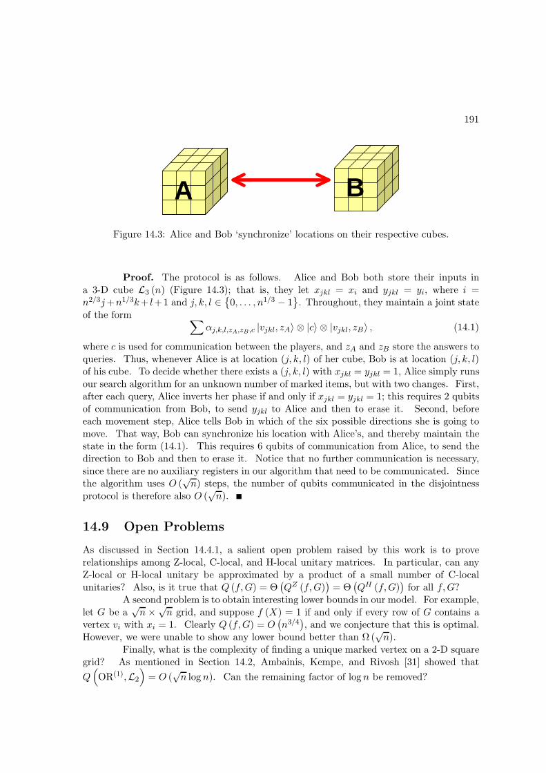
191

A BA B

Figure 14.3: Alice and Bob ‘synchronize’ locations on their respective cubes.

Proof. The protocol is as follows. Alice and Bob both store their inputs ina 3-D cube L3 (n) (Figure 14.3); that is, they let xjkl = xi and yjkl = yi, where i =n2/3j+n1/3k+ l+1 and j, k, l ∈

0, . . . , n1/3 − 1

. Throughout, they maintain a joint state

of the form ∑αj,k,l,zA,zB,c |vjkl, zA〉 ⊗ |c〉 ⊗ |vjkl, zB〉 , (14.1)

where c is used for communication between the players, and zA and zB store the answers toqueries. Thus, whenever Alice is at location (j, k, l) of her cube, Bob is at location (j, k, l)of his cube. To decide whether there exists a (j, k, l) with xjkl = yjkl = 1, Alice simply runsour search algorithm for an unknown number of marked items, but with two changes. First,after each query, Alice inverts her phase if and only if xjkl = yjkl = 1; this requires 2 qubitsof communication from Bob, to send yjkl to Alice and then to erase it. Second, beforeeach movement step, Alice tells Bob in which of the six possible directions she is going tomove. That way, Bob can synchronize his location with Alice’s, and thereby maintain thestate in the form (14.1). This requires 6 qubits of communication from Alice, to send thedirection to Bob and then to erase it. Notice that no further communication is necessary,since there are no auxiliary registers in our algorithm that need to be communicated. Sincethe algorithm uses O (

√n) steps, the number of qubits communicated in the disjointness

protocol is therefore also O (√n).

14.9 Open Problems

As discussed in Section 14.4.1, a salient open problem raised by this work is to proverelationships among Z-local, C-local, and H-local unitary matrices. In particular, can anyZ-local or H-local unitary be approximated by a product of a small number of C-localunitaries? Also, is it true that Q (f,G) = Θ

(QZ (f,G)

)= Θ

(QH (f,G)

)for all f,G?

A second problem is to obtain interesting lower bounds in our model. For example,let G be a

√n × √

n grid, and suppose f (X) = 1 if and only if every row of G contains avertex vi with xi = 1. Clearly Q (f,G) = O

(n3/4

), and we conjecture that this is optimal.

However, we were unable to show any lower bound better than Ω (√n).

Finally, what is the complexity of finding a unique marked vertex on a 2-D squaregrid? As mentioned in Section 14.2, Ambainis, Kempe, and Rivosh [31] showed that

Q(OR(1),L2

)= O (

√n log n). Can the remaining factor of log n be removed?

192

Chapter 15

Quantum Computing andPostselection

“Gill, in his seminal paper on probabilistic complexity classes, defined the classPP and asked whether the class was closed under intersection. In 1990, Fennerand Kurtz and later myself, decided to try a new approach to the question:Consider a class defined like PP but with additional restrictions, show that thisclass is closed under intersection and then show the class was really the same asPP.”

—Lance Fortnow, My Computational Complexity Web Log [115]

(the approach didn’t succeed, though as this chapter will show, all it was missingwas quantum mechanics)

Postselection is the power of discarding all runs of a computation in which a givenevent does not occur. Clearly, such an ability would let us solve NP-complete problems inpolynomial time, since we could guess a random solution, and then postselect on its beingcorrect. But would postselection let us do more than NP? Using a classical computer, theclass of problems we could efficiently solve coincides with a class called BPPpath, which wasdefined by Han, Hemaspaandra, and Thierauf [144] and which sits somewhere between MA

and PP.This chapter studies the power of postselection when combined with quantum

computing. In Section 15.1, I define a new complexity class called PostBQP, which issimilar to BQP except that we can measure a qubit that has some nonzero probability ofbeing |1〉, and assume the outcome will be |1〉. The main result is that PostBQP equalsthe classical complexity class PP.

My original motivation, which I explain in Section 15.2, was to analyze the com-putational power of “fantasy” versions of quantum mechanics, and thereby gain insight intowhy quantum mechanics is the way it is. For example, I show in Section 15.2 that if wechanged the measurement probability rule from |ψ|2 to |ψ|p for some p 6= 2, or allowed linearbut nonunitary gates, then we could simulate postselection, and hence solve PP-completeproblems in polynomial time. I was also motivated by a concept that I call anthropic com-puting : arranging things so that you’re more likely to exist if a computer produces a desired

193

output than if it doesn’t. As a simple example, under the many-worlds interpretation ofquantum mechanics, you might kill yourself in all universes where a computer’s output isincorrect. My result implies that, using this “technique,” the class of problems that youcould efficiently solve is exactly PP.

However, it recently dawned on me that the PostBQP = PP result is also in-teresting for purely classical reasons. In particular, it yields an almost-trivial, quantumcomputing based proof that PP is closed under intersection. This proof does not use ra-tional approximations, threshold polynomials, or any of the other techniques pioneered byBeigel, Reingold, and Spielman [47] in their justly-celebrated original proof. Another im-mediate corollary of my new characterization of PP is a result originally due to Fortnow andReingold [117]: that PP is closed under polynomial-time truth-table reductions. Indeed, Ican show that PP is closed under BQP truth-table reductions, which is a new result as faras I know. I conclude in Section 15.3 with some open problems.

15.1 The Class PostBQP

I hereby define a complexity class:

Definition 132 PostBQP (Postselected Bounded-Error Quantum Polynomial-Time) is theclass of languages L for which there exists a uniform family of polynomial-size quantumcircuits such that for all inputs x,

(i) At the end of the computation, the first qubit has a nonzero probability of being mea-sured to be |1〉.

(ii) If x ∈ L, then conditioned on the first qubit being |1〉, the second qubit is |1〉 withprobability at least 2/3.

(iii) If x /∈ L, then conditioned on the first qubit being |1〉, the second qubit is |1〉 withprobability at most 1/3.

We can think of PostBQP as the “nondeterministic” version of BQP. Admittedly,there are already three other contenders for that title: QMA, defined by Watrous [239];QCMA, defined by Aharonov and Naveh [21]; and NQP, defined by Adleman, DeMarrais,and Huang [16] (which turns out to equal coC=P [109]). As we will see, PostBQP containsall of these as subclasses.

It is immediate that NP ⊆ PostBQP ⊆ PP. For the latter inclusion, we can usethe same techniques used by Adleman, DeMarrais, and Huang [16] to show that BQP ⊆ PP,but sum only over paths where the first qubit is |1〉 at the end. This is made explicit inTheorem 57 of Chapter 10.

How robust is PostBQP? Just as Bernstein and Vazirani [55] showed that in-termediate measurements don’t increase the power of ordinary quantum computers, so it’seasy to show that intermediate postselection steps don’t increase the power of PostBQP.Whenever we want to postselect on a qubit being |1〉, we simply CNOT that qubit into afresh ancilla qubit that is initialized to |0〉 and that will never be written to again. Then,at the end, we compute the AND of all the ancilla qubits, and swap the result into the

194

first qubit. It follows that we can repeat a PostBQP computation a polynomial number oftimes, and thereby amplify the probability gap from (1/3, 2/3) to

(2−p(n), 1 − 2−p(n)

)for

any polynomial p.A corollary of the above observations is that PostBQP has strong closure properties.

Proposition 133 PostBQP is closed under union, intersection, and complement. Indeed,it is closed under BQP truth table reductions, meaning that PostBQP = BQPPostBQP

‖, classical, where

BQPPostBQP‖, classical is the class of problems solvable by a BQP machine that can make a polynomial

number of nonadaptive classical queries to a PostBQP oracle.

Proof. Clearly PostBQP is closed under complement. To show closure underintersection, let L1, L2 ∈ PostBQP. Then to decide whether x ∈ L1 ∩ L2, run amplifiedcomputations (with error probability at most 1/6) to decide if x ∈ L1 and if x ∈ L2,postselect on both computations succeeding, and accept if and only if both accept. Itfollows that PostBQP is closed under union as well.

In general, suppose a BQPPostBQP‖, classical machine M submits queries q1, . . . , qp(n) to the

PostBQP oracle. Then run amplified computations (with error probability at most, say,1

10p(n)) to decide the answers to these queries, and postselect on all p (n) of them succeeding.By the union bound, if M had error probability ε with a perfect PostBQP oracle, then itsnew error probability is at most ε+1/10, which can easily be reduced through amplification.

One might wonder why Proposition 133 doesn’t go through with adaptive queries.The reason is subtle: suppose we have two PostBQP computations, the second of which relieson the output of the first. Then even if the first computation is amplified a polynomialnumber of times, it still has an exponentially small probability of error. But since thesecond computation uses postselection, any nonzero error probability could be magnifiedarbitrarily, and is therefore too large.

I now prove the main result.

Theorem 134 PostBQP = PP.

Proof. We have already observed that PostBQP ⊆ PP. For the other di-rection, let f : 0, 1n → 0, 1 be an efficiently computable Boolean function and lets = |x : f (x) = 1|. Then we need to decide in PostBQP whether s < 2n−1 or s ≥ 2n−1.(As a technicality, we can guarantee using padding that s > 0.)

The algorithm is as follows: first prepare the state 2−n/2∑

x∈0,1n |x〉 |f (x)〉.Then following Abrams and Lloyd [15], apply Hadamard gates to all n qubits in the firstregister and postselect1 on that register being |0〉⊗n, to obtain |0〉⊗n |ψ〉 where

|ψ〉 =(2n − s) |0〉 + s |1〉√

(2n − s)2 + s2.

1Postselection is actually overkill here, since the first register has at least 1/4 probability of being |0〉⊗n.

195

+1

0

Figure 15.1: If s and 2n − 2s are both positive, then as we vary the ratio of β to α, weeventually get close to |+〉 = (|0〉 + |1〉) /

√2 (dashed lines). On the other hand, if 2n − 2s

is not positive (dotted line), then we never even get into the first quadrant.

Next, for some positive real numbers α, β to be specified later, prepare α |0〉 |ψ〉+β |1〉H |ψ〉where

H |ψ〉 =

√1/2 (2n) |0〉 +

√1/2 (2n − 2s) |1〉√

(2n − s)2 + s2

is the result of applying a Hadamard gate to |ψ〉. Then postselect on the second qubitbeing |1〉. This yields the reduced state

∣∣ϕβ/α⟩

=αs |0〉 + β

√1/2 (2n − 2s) |1〉√

α2s2 + (β2/2) (2n − 2s)2

in the first qubit.Suppose s < 2n−1, so that s and

√1/2 (2n − 2s) are both at least 1. Then we

claim there exists an integer i ∈ [−n, n] such that, if we set β/α = 2i, then |ϕ2i〉 is close tothe state |+〉 = (|0〉 + |1〉) /

√2:

|〈+|ϕ2i〉| ≥ 1 +√

2√6

> 0.985.

For since√

1/2 (2n − 2s) /s lies between 2−n and 2n, there must be an integer i ∈ [−n, n− 1]such that |ϕ2i〉 and |ϕ2i+1〉 fall on opposite sides of |+〉 in the first quadrant (see Figure15.1). So the worst case is that 〈+|ϕ2i〉 = 〈+|ϕ2i+1〉, which occurs when |ϕ2i〉 =

√2/3 |0〉+√

1/3 |0〉 and |ϕ2i+1〉 =√

1/3 |0〉+√

2/3 |0〉. On the other hand, suppose s ≥ 2n−1, so that√1/2 (2n − 2s) ≤ 0. Then |ϕ2i〉 never lies in the first or third quadrants, and therefore

|〈+|ϕ2i〉| ≤ 1/√

2 < 0.985.

196

It follows that, by repeating the whole algorithm n (2n + 1) times (as in Proposi-tion 133), with n invocations for each integer i ∈ [−n, n], we can learn whether s < 2n−1 ors ≥ 2n−1 with exponentially small probability of error.

Combining Proposition 133 with Theorem 134 immediately yields that PP is closedunder intersection, as well as under BQP truth-table reductions.

15.2 Fantasy Quantum Mechanics

“It is striking that it has so far not been possible to find a logically consis-tent theory that is close to quantum mechanics, other than quantum mechanicsitself.”

—Steven Weinberg, Dreams of a Final Theory [241]

Is quantum mechanics an island in theoryspace? By “theoryspace,” I mean thespace of logically conceivable physical theories, with two theories close to each other if theydiffer in few respects. An “island” in theoryspace is then a natural and interesting theory,whose neighbors are all somehow perverse or degenerate. The Standard Model is not anisland, because we do not know of any compelling (non-anthropic) reason why the massesand coupling constants should have the values they do. Likewise, general relativity isprobably not an island, because of alternatives such as the Brans-Dicke theory.

To many physicists, however, quantum mechanics does seem like an island: changeany one aspect, and the whole theory becomes inconsistent or nonsensical. There are manymathematical results supporting this opinion: for example, Gleason’s Theorem [129] andother “derivations” of the |ψ|2 probability rule [95, 252]; arguments for why amplitudes haveto be complex numbers, rather than real numbers or quaternions [81, 145]; and “absurd”consequences of allowing nonlinear transformations between states [15, 128, 193]. Thepoint of these results is to provide some sort of explanation for why quantum mechanicshas the properties it does.

In 1998, Abrams and Lloyd [15] suggested that computational complexity couldalso be pressed into such an explanatory role. In particular, they showed that underalmost any nonlinear variant of quantum mechanics, one could build a “nonlinear quantumcomputer” able to solve NP-complete and even #P-complete problems in polynomial time.2

One interpretation of their result is that we should look very hard for nonlinearities inexperiments! But a different interpretation, the one I prefer, is that their result providesindependent evidence that quantum mechanics is linear.3

2A caveat is that it remains an open problem whether this can be done fault-tolerantly. The answermight depend on the allowed types of nonlinear gate. On the other hand, if arbitrary 1-qubit nonlineargates can be implemented without error, then even PSPACE-complete problems can be solved in polynomialtime. This is tight, since nonlinear quantum computers can also be simulated in PSPACE. I will give moredetails in a forthcoming survey paper [12].

3Note that I would not advocate this interpretation if it was merely (say) graph isomorphism thatwas efficiently solvable in nonlinear quantum mechanics, just as I do not take Shor’s factoring algorithm asevidence for the falsehood of ordinary quantum mechanics. I will explain in [12] why I think this distinction,between NP-complete problems and specific NP-intermediate problems, is a justified one.

197

In this section I build on Theorem 134 to offer similar “evidence” that quantummechanics is unitary, and that the measurement rule is |ψ|2.

Let BQPnu be the class of problems solvable by a uniform family of polynomial-size,bounded-error quantum circuits, where the circuits can consist of arbitrary 1- and 2-qubitinvertible linear transformations, rather than just unitary transformations. Immediately

before a measurement, the amplitude αx of each basis state |x〉 is divided by√∑

y |αy|2 to

normalize it.

Proposition 135 BQPnu

= PP.

Proof. The inclusion BQPnu ⊆ PP follows easily from Adleman, DeMarrais, andHuang’s proof that BQP ⊆ PP [16], which does not depend on unitarity. For the otherdirection, by Theorem 134 it suffices to show that PostBQP ⊆ BQPnu. To postselect on aqubit being |1〉, we simply apply the 1-qubit nonunitary operation

(2−q(n) 0

0 1

)

for some sufficiently large polynomial q.Next, for any nonnegative real number p, define BQPp similarly to BQP, except

that when we measure, the probability of obtaining a basis state |x〉 equals |αx|p /∑

y |αy|prather than |αx|2. Thus BQP2 = BQP. Assume that all gates are unitary and that thereare no intermediate measurements, just a single standard-basis measurement at the end.

Theorem 136 PP ⊆ BQPp ⊆ PSPACE for all constants p 6= 2, with BQPp = PP whenp ∈ 4, 6, 8, . . ..

Proof. To simulate PP in BQPp, run the algorithm of Theorem 134, having

initialized O(

1|p−2| poly (n)

)ancilla qubits to |0〉. Suppose the algorithm’s state at some

point is∑

x αx |x〉, and we want to postselect on the event |x〉 ∈ S, where S is a subset ofbasis states. Here is how: if p < 2, then for some sufficiently large polynomial q, applyHadamard gates to c = 2q (n) / (2 − p) fresh ancilla qubits conditioned on |x〉 ∈ S. Theresult is to increase the “probability mass” of each |x〉 ∈ S from |αx|p to

2c ·∣∣∣2−c/2αx

∣∣∣p

= 2(2−p)c/2 |αx|p = 2q(n) |αx|p ,

while the probability mass of each |x〉 /∈ S remains unchanged. Similarly, if p > 2, thenapply Hadamard gates to c = 2q (n) / (p− 2) fresh ancilla qubits conditioned on |x〉 /∈S. This decreases the probability mass of each |x〉 /∈ S from |αx|p to 2c ·

∣∣2−c/2αx∣∣p =

2−q(n) |αx|p, while the probability mass of each |x〉 ∈ S remains unchanged. The finalobservation is that Theorem 134 still goes through if p 6= 2. For it suffices to distinguishthe case |〈+|ϕ2i〉| > 0.985 from |〈+|ϕ2i〉| ≤ 1/

√2 with exponentially small probability of

error, using polynomially many copies of the state |ϕ2i〉. But we can do this for any p,since all |ψ|p rules behave well under tensor products (in the sense that |αβ|p = |α|p |β|p).

198

The inclusion BQPp ⊆ PSPACE follows easily from the techniques used by Bern-stein and Vazirani [55] to show BQP ⊆ PSPACE. Let S be the set of accepting states; thensimply compute

∑x∈S |αx|p and

∑x/∈S |αx|p and see which is greater.

To simulate BQPp in PP when p ∈ 4, 6, 8, . . ., we generalize the technique ofAdleman, DeMarrais, and Huang [16], which handled the case p = 2. As in Theorem 57 inChapter 10, assume that all gates are Hadamard or Toffoli gates; then we can write eachamplitude αx as a sum of exponentially many contributions, ax,1 + · · · + ax,N , where eachax,i is a rational real number computable in classical polynomial time. Then letting S bethe set of accepting states, it suffices to test whether

∑

x∈S|αx|p =

∑

x∈Sαpx

=∑

x∈S

∑

i∈1,...,Nax,i

p

=∑

x∈S

∑

B⊆1,...,N,|B|=p

∏

i∈Bax,i

is greater than∑

x/∈S |αx|p, which we can do in PP.

15.3 Open Problems

The new proof that PP is closed under intersection came as a total surprise to me. But onreflection, it goes a long way toward convincing me of a thesis expressed in Chapter 1: thatquantum computing offers a new perspective from which to revisit the central questions ofclassical complexity theory. What other classical complexity classes can we characterize inquantum terms, and what other questions can we answer by that means?

A first step might be to prove even stronger closure properties for PP. Recallfrom Proposition 133 that PostBQP is closed under polynomial-time truth-table reductions.Presumably this can’t be generalized to closure under Turing reductions, since if it couldthen we would have PP = PPP, which is considered unlikely.4 But can we show closureunder nonadaptive quantum reductions? More formally, let BQPPostBQP

‖ be the class ofproblems solvable by a BQP machine that can make a single quantum query, which consistsof a list of polynomially many questions for a PostBQP oracle. Then does BQPPostBQP

‖equal PostBQP? The difficulty in showing this seems to be uncomputing garbage after thePostBQP oracle is simulated.

As for fantasy quantum mechanics, an interesting open question is whether BQPp =PP for all nonnegative real numbers p 6= 2. An obvious idea for simulating BQPp in PP

would be to use a Taylor series expansion for the probability masses |αx|p. Unfortunately,I have no idea how to get fast enough convergence.

4Indeed, Beigel [46] gave an oracle relative to which PNP 6⊂ PP.

199

Chapter 16

The Power of History

Quantum mechanics lets us calculate the probability that (say) an electron willbe found in an excited state if measured at a particular time. But it is silent aboutmultiple-time or transition probabilities: that is, what is the probability that the electronwill be in an excited state at time t1, given that it was in its ground state at an earliertime t0? The usual response is that this question is meaningless, unless of course theelectron was measured (or otherwise known with probability 1) to be in its ground stateat t0. A different response—pursued by Schrodinger [215], Bohm [59], Bell [49], Nelson[183], Dieks [99], and others—treats the question as provisionally meaningful, and theninvestigates how one might answer it mathematically. Specific attempts at answers arecalled “hidden-variable theories.”

The appeal of hidden-variable theories is that they provide one possible solution tothe measurement problem. For they allow us to apply unitary quantum mechanics to theentire universe (including ourselves), yet still discuss the probability of a future observationconditioned on our current observations. Furthermore, they let us do so without makingany assumptions about decoherence or the nature of observers. For example, even if anobserver were placed in coherent superposition, that observer would still have a sequenceof definite experiences, and the probability of any such sequence could be calculated.

This chapter initiates the study of hidden variables from a quantum computingperspective. I restrict attention to the simplest possible setting: that of discrete time,a finite-dimensional Hilbert space, and a fixed orthogonal basis. Within this setting, Ireformulate known hidden-variable theories due to Dieks [99] and Schrodinger [215], and alsointroduce a new theory based on network flows. However, a more important contributionis the axiomatic approach that I use. I propose five axioms for hidden-variable theories,and then compare theories against each other based on which of the axioms they satisfy. Acentral question in this approach is which subsets of axioms can be satisfied simultaneously.

In a second part of the chapter, I make the connection to quantum computingexplicit, by studying the computational complexity of simulating hidden-variable theories.Below I describe the computational results.

200

16.1 The Complexity of Sampling Histories

It is often stressed that hidden-variable theories yield exactly the same predictions as ordi-nary quantum mechanics. On the other hand, these theories describe a different picture ofphysical reality, with an additional layer of dynamics beyond that of a state vector evolvingunitarily. I address a question that, to my knowledge, had never been raised before: whatis the computational complexity of simulating that additional dynamics? In other words,if we could examine a hidden variable’s entire history, then could we solve problems inpolynomial time that are intractable even for quantum computers?

I present strong evidence that the answer is yes. The Graph Isomorphism problemasks whether two graphs G and H are isomorphic; while given a basis for a lattice L ∈ Rn,the Approximate Shortest Vector problem asks for a nonzero vector in L within a

√n

factor of the shortest one. I show that both problems are efficiently solvable by sampling ahidden variable’s history, provided the hidden-variable theory satisfies a reasonable axiom.By contrast, despite a decade of effort, neither problem is known to lie in BQP. Thus,if we let DQP (Dynamical Quantum Polynomial-Time) be the class of problems solvablein the new model, then this already provides circumstantial evidence that BQP is strictlycontained in DQP.

However, the evidence is stronger than this. For I actually show that DQP containsthe entire class Statistical Zero Knowledge, or SZK. Furthermore, Chapter 6 showed thatrelative to an oracle, SZK is not contained in BQP. Combining the result that SZK ⊆ DQP

with the oracle separation of Chapter 6, one obtains that BQP 6= DQP relative to an oracleas well.

Besides solving SZK problems, I also show that by sampling histories, one couldsearch an unordered database of N items for a single “marked item” using only O

(N1/3

)

database queries. By comparison, Grover’s quantum search algorithm [141] requires Θ(N1/2

)

queries, while classical algorithms require Θ (N) queries. On the other hand, I also showthat the N1/3 upper bound is the best possible—so even in the histories model, one cannotsearch an N -item database in (logN)c steps for some fixed power c. This implies thatNP 6⊂ DQP relative to an oracle, which in turn suggests that DQP is still not powerfulenough to solve NP-complete problems in polynomial time.

At this point I should address a concern that many readers will have. Once weextend quantum mechanics by positing the “unphysical” ability to sample histories, isn’t itcompletely unsurprising if we can then solve problems that were previously intractable? Ibelieve the answer is no, for three reasons.

First, almost every change that makes the quantum computing model more pow-erful, seems to make it so much more powerful that NP-complete and even harder problemsbecome solvable efficiently. To give some examples, NP-complete problems can be solvedin polynomial time using a nonlinear Schrodinger equation, as shown by Abrams and Lloyd[15]; using closed timelike curves, as shown by Brun [72] and Bacon [40] (and conjecturedby Deutsch [93]); or using a measurement rule of the form |ψ|p for any p 6= 2, as shown inChapter 15. It is also easy to see that we could solve NP-complete problems if, given aquantum state |ψ〉, we could request a classical description of |ψ〉, such as a list of ampli-

201

tudes or a preparation procedure.1 By contrast, the DQP model is the first independentlymotivated model I know of that seems more powerful than quantum computing, but onlyslightly so.2 Moreover, the striking fact that unordered search takes about N1/3 steps inthe DQP model, as compared to N steps classically and N1/2 quantum-mechanically, sug-gests that DQP somehow “continues a sequence” that begins with P and BQP. It wouldbe interesting to find a model in which search takes N1/4 or N1/5 steps.

The second reason the results are surprising is that, given a hidden variable, thedistribution over its possible values at any single time is governed by standard quantummechanics, and is therefore efficiently samplable on a quantum computer. So if examiningthe variable’s history confers any extra computational power, then it can only be becauseof correlations between the variable’s values at different times.

The third reason is the criterion for success. I am not saying merely that onecan solve Graph Isomorphism under some hidden-variable theory; or even that, under anytheory satisfying the indifference axiom, there exists an algorithm to solve it; but rather thatthere exists a single algorithm that solves Graph Isomorphism under any theory satisfyingindifference. Thus, we must consider even theories that are specifically designed to thwartsuch an algorithm.

But what is the motivation for these results? The first motivation is that, withinthe community of physicists who study hidden-variable theories such as Bohmian mechan-ics, there is great interest in actually calculating the hidden-variable trajectories for specificphysical systems [192, 142]. My results show that, when many interacting particles areinvolved, this task might be fundamentally intractable, even if a quantum computer wereavailable. The second motivation is that, in classical computer science, studying “unreal-istic” models of computation has often led to new insights into realistic ones; and likewise Iexpect that the DQP model could lead to new results about standard quantum computation.Indeed, in a sense this has already happened—for the collision lower bound of Chapter 6grew out of work on the BQP versus DQP question.

16.2 Outline of Chapter

Sections 16.3 through 16.6 develop the axiomatic approach to hidden variables; then Sec-tions 16.7 through 16.10 study the computational complexity of sampling hidden-variablehistories.

Section 16.3 formally defines hidden-variable theories in my sense; then Section16.3.1 contrasts these theories with related ideas such as Bohmian mechanics and modalinterpretations. Section 16.3.2 addresses the most common objections to my approach: forexample, that the implicit dependence on a fixed basis is unacceptable.

In Section 16.4, I introduce five possible axioms for hidden-variable theories. Theseare indifference to the identity operation; robustness to small perturbations; commutativity

1For as Abrams and Lloyd [15] observed, we can so arrange things that |ψ〉 = |0〉 if an NP-completeinstance of interest to us has no solution, but |ψ〉 =

√1 − ε |0〉 +

√ε |1〉 for some tiny ε if it has a solution.

2One can define other, less motivated, models with the same property by allowing “non-collapsing mea-surements” of quantum states, but these models are very closely related to DQP. Indeed, a key ingredientin the results of this chapter will be to show that certain kinds of non-collapsing measurements can besimulated using histories.

202

with respect to spacelike-separated unitaries; commutativity for the special case of productstates; and invariance under decomposition of mixed states into pure states. Ideally, atheory would satisfy all of these axioms. However, I show in Section 16.5 that no theorysatisfies both indifference and commutativity; no theory satisfies both indifference and astronger version of robustness; no theory satisfies indifference, robustness, and decomposi-tion invariance; and no theory satisfies a stronger version of decomposition invariance.

In Section 16.6 I shift from negative to positive results. Section 16.6.1 presents ahidden-variable theory called the flow theory or FT , which is based on the Max-Flow-Min-Cut theorem from combinatorial optimization. The idea is to define a network of “pipes”from basis states at an initial time to basis states at a final time, and then route as muchprobability mass as possible through these pipes. The capacity of each pipe depends onthe corresponding entry of the unitary acting from the initial to final time. To find theprobability of transitioning from basis state |i〉 to basis state |j〉, we then determine howmuch of the flow originating at |i〉 is routed along the pipe to |j〉. The main results arethat FT is well-defined and that it is robust to small perturbations. Since FT triviallysatisfies the indifference axiom, this implies that the indifference and robustness axioms canbe satisfied simultaneously, which was not at all obvious a priori.

Section 16.6.2 presents a second theory that I call the Schrodinger theory or ST ,since it is based on a pair of integral equations introduced in a 1931 paper of Schrodinger[215]. Schrodinger conjectured, but was unable to prove, the existence and uniqueness of asolution to these equations; the problem was not settled until the work of Nagasawa [181]in the 1980’s. In the discrete setting the problem is simpler, and I give a self-containedproof of existence using a matrix scaling technique due to Sinkhorn [223]. The idea is asfollows: we want to convert a unitary matrix that maps one quantum state to another, intoa nonnegative matrix whose ith column sums to the initial probability of basis state |i〉, andwhose jth row sums to the final probability of basis state |j〉. To do so, we first replace eachentry of the unitary matrix by its absolute value, then normalize each column to sum to thedesired initial probability, then normalize each row to sum to the desired final probability.But then the columns are no longer normalized correctly, so we normalize them again, thennormalize the rows again, and so on. I show that this iterative process converges, fromwhich it follows that ST is well-defined. I also observe that ST satisfies the indifferenceand product commutativity axioms, and violates the decomposition invariance axiom. Iconjecture that ST satisfies the robustness axiom; proving that conjecture is one of themain open problems of the chapter.

In Section 16.7 I shift attention to the complexity of sampling histories. I formallydefine DQP as the class of problems solvable by a classical polynomial-time algorithm withaccess to a “history oracle.” Given a sequence of quantum circuits as input, this oraclereturns a sample from a corresponding distribution over histories of a hidden variable,according to some hidden-variable theory T . The oracle can choose T “adversarially,”subject to the constraint that T satisfies the indifference and robustness axioms. Thus,a key result from Section 16.7 that I rely on is that there exists a hidden-variable theorysatisfying indifference and robustness.

Section 16.7.1 establishes the most basic facts about DQP: for example, thatBQP ⊆ DQP, and that DQP is independent of the choice of gate set. Then Section 16.8

203

presents the “juggle subroutine,” a crucial ingredient in both of the main hidden-variablealgorithms. Given a state of the form (|a〉 + |b〉) /

√2 or (|a〉 − |b〉) /

√2, the goal of this

subroutine is to “juggle” a hidden variable between |a〉 and |b〉, so that when we inspect thehidden variable’s history, both |a〉 and |b〉 are observed with high probability. The difficultyis that this needs to work under any indifferent hidden-variable theory.

Next, Section 16.9 combines the juggle subroutine with a technique of Valiant andVazirani [233] to prove that SZK ⊆ DQP, from which it follows in particular that GraphIsomorphism and Approximate Shortest Vector are in DQP. Then Section 16.10 appliesthe juggle subroutine to search an N -item database in O

(N1/3

)queries, and also proves

that this N1/3 bound is optimal.I conclude in Section 16.11 with some directions for further research.

16.3 Hidden-Variable Theories

Suppose we have an N ×N unitary matrix U , acting on a state

|ψ〉 = α1 |1〉 + · · · + αN |N〉 ,

where |1〉 , . . . , |N〉 is a standard orthogonal basis. Let

U |ψ〉 = β1 |1〉 + · · · + βN |N〉 .

Then can we construct a stochastic matrix S, which maps the vector of probabilities

−→p =

|α1|2...

|αN |2

induced by measuring |ψ〉, to the vector

−→q =

|β1|2...

|βN |2

induced by measuring U |ψ〉? Trivially yes. The following matrix maps any vector ofprobabilities to −→q , ignoring the input vector −→p entirely:

SPT =

|β1|2 · · · |β1|2...

...

|βN |2 · · · |βN |2

.

Here PT stands for product theory. The product theory corresponds to a strange pictureof physical reality, in which memories and records are completely unreliable, there being nocausal connection between states of affairs at earlier and later times.

So we would like S to depend on U itself somehow, not just on |ψ〉 and U |ψ〉.Indeed, ideally S would be a function only of U , and not of |ψ〉. But this is impossible, as

204

the following example shows. Let U be a π/4 rotation, and let |+〉 = (|0〉 + |1〉) /√

2 and|−〉 = (|0〉 − |1〉) /

√2. Then U |+〉 = |1〉 implies that

S (|+〉 , U) =

[0 01 1

],

whereas U |−〉 = |0〉 implies that

S (|−〉 , U) =

[1 10 0

].

On the other hand, it is easy to see that, if S can depend on |ψ〉 as well as U ,then there are infinitely many choices for the function S (|ψ〉 , U). Every choice reproducesthe predictions of quantum mechanics perfectly when restricted to single-time probabilities.So how can we possibly choose among them? My approach in Sections 16.4 and 16.6 willbe to write down axioms that we would like S to satisfy, and then investigate which of theaxioms can be satisfied simultaneously.

Formally, a hidden-variable theory is a family of functions SNN≥1, where eachSN maps an N -dimensional mixed state ρ and an N ×N unitary matrix U onto a singlystochastic matrix SN (ρ, U). I will often suppress the dependence on N , ρ, and U , andoccasionally use subscripts such as PT or FT to indicate the theory in question. Also, ifρ = |ψ〉〈ψ| is a pure state I may write S (|ψ〉 , U) instead of S (|ψ〉〈ψ| , U).

Let (M)ij denote the entry in the ith column and jth row of matrix M . Then (S)ijis the probability that the hidden variable takes value |j〉 after U is applied, conditionedon it taking value |i〉 before U is applied. At a minimum, any theory must satisfy thefollowing marginalization axiom: for all j ∈ 1, . . . , N,

∑

i

(S)ij (ρ)ii =(UρU−1

)jj

.

This says that after U is applied, the hidden variable takes value |j〉 with probability(UρU−1

)jj

, which is the usual Born probability.

Often it will be convenient to refer, not to S itself, but to the matrix P (ρ, U) ofjoint probabilities whose (i, j) entry is (P )ij = (S)ij (ρ)ii. The ith column of P must sum

to (ρ)ii, and the jth row must sum to(UρU−1

)jj

. Indeed, I will define the theories FT and

ST by first specifying the matrix P , and then setting (S)ij := (P )ij / (ρ)ii. This approach

has the drawback that if (ρ)ii = 0, then the ith column of S is undefined. To get aroundthis, I adopt the convention that

S (ρ, U) := limε→0+

S (ρε, U)

where ρε = (1 − ε) ρ + εI and I is the N × N maximally mixed state. Technically, thelimits

limε→0+

(P (ρε, U))ij(ρε)ii

might not exist, but in the cases of interest it will be obvious that they do.

205

16.3.1 Comparison with Previous Work

Before going further, I should contrast my approach with previous approaches to hiddenvariables, the most famous of which is Bohmian mechanics [59]. My main difficulty withBohmian mechanics is that it commits itself to a Hilbert space of particle positions andmomenta. Furthermore, it is crucial that the positions and momenta be continuous, inorder for particles to evolve deterministically. To see this, let |L〉 and |R〉 be discretepositions, and suppose a particle is in state |L〉 at time t0, and state (|L〉 + |R〉) /

√2 at

a later time t1. Then a hidden variable representing the position would have entropy 0at t1, since it is always |L〉 then; but entropy 1 at t1, since it is |L〉 or |R〉 both with1/2 probability. Therefore the earlier value cannot determine the later one.3 It followsthat Bohmian mechanics is incompatible with the belief that all physical observables arediscrete. But in my view, there are strong reasons to hold that belief, which include blackhole entropy bounds; the existence of a natural minimum length scale (10−33 cm); resultson area quantization in quantum gravity [207]; the fact that many physical quantities oncethought to be continuous have turned out to be discrete; the infinities of quantum fieldtheory; the implausibility of analog “hypercomputers”; and conceptual problems raised bythe independence of the continuum hypothesis.

Of course there exist stochastic analogues of Bohmian mechanics, among themNelsonian mechanics [183] and Bohm and Hiley’s “stochastic interpretation” [60]. But it isnot obvious why we should prefer these to other stochastic hidden-variable theories. Froma quantum-information perspective, it is much more natural to take an abstract approach—one that allows arbitrary finite-dimensional Hilbert spaces, and that does not rule out anytransition rule a priori.

Stochastic hidden variables have also been considered in the context of modalinterpretations; see Dickson [98], Bacciagaluppi and Dickson [39], and Dieks [99] for example.However, the central assumptions in that work are extremely different from mine. Inmodal interpretations, a pure state evolving unitarily poses no problems at all: one simplyrotates the hidden-variable basis along with the state, so that the state always representsa “possessed property” of the system in the current basis. Difficulties arise only for mixedstates; and there, the goal is to track a whole set of possessed properties. By contrast, myapproach is to fix an orthogonal basis, then track a single hidden variable that is an elementof that basis. The issues raised by pure states and mixed states are essentially the same.

Finally I should mention the consistent-histories interpretation of Griffiths [139]and Gell-Mann and Hartle [124]. This interpretation assigns probabilities to various his-tories through a quantum system, so long as the “interference” between those histories isnegligible. Loosely speaking, then, the situations where consistent histories make sense areprecisely the ones where the question of transition probabilities can be avoided.

3Put differently, Bohm’s conservation of probability result breaks down because the “wavefunctions” att0 and t1 are degenerate, with all amplitude concentrated on finitely many points. But in a discrete Hilbertspace, every wavefunction is degenerate in this sense!

206

16.3.2 Objections

Hidden-variable theories, as I define them, are open to several technical objections. Forexample, I required transition probabilities for only one orthogonal observable. Whatabout other observables? The problem is that, according to the Kochen-Specker theorem,we cannot assign consistent values to all observables at any single time, let alone givetransition probabilities for those values. This is an issue in any setting, not just mine. Thesolution I prefer is to postulate a fixed orthogonal basis of “distinguishable experiences,”and to interpret a measurement in any other basis as a unitary followed by a measurementin the fixed basis. As mentioned in Section 16.3.1, modal interpretations opt for a differentsolution, which involves sets of bases that change over time with the state itself.

Another objection is that the probability of transitioning from basis state |i〉 attime t1 to basis state |j〉 at time t2 might depend on how finely we divide the time intervalbetween t1 and t2. In other words, for some state |ψ〉 and unitaries V,W , we might have

S (|ψ〉 ,WV ) 6= S (V |ψ〉 ,W )S (|ψ〉 , V )

(a similar point was made by Gillespie [127]). Indeed, this is true for any hidden-variabletheory other than the product theory PT . To see this, observe that for all unitaries U andstates |ψ〉, there exist unitaries V,W such that U = WV and V |ψ〉 = |1〉. Then applyingV destroys all information in the hidden variable (that is, decreases its entropy to 0); soif we then apply W , then the variable’s final value must be uncorrelated with the initialvalue. In other words, S (V |ψ〉 ,W )S (|ψ〉 , V ) must equal SPT (|ψ〉 , U). It follows that toany hidden-variable theory we must associate a time scale, or some other rule for decidingwhen the transitions take place.

In response, it should be noted that exactly the same problem arises in continuous-time stochastic hidden-variable theories. For if a state |ψ〉 is governed by the Schrodingerequation d |ψ〉 /dt = iHt |ψ〉, and a hidden variable’s probability distribution −→p is governedby the stochastic equation d−→p /dτ = Aτ

−→p , then there is still an arbitrary parameter dτ/dton which the dynamics depend.

Finally, it will be objected that I have ignored special relativity. In Section 16.4I will define a commutativity axiom, which informally requires that the stochastic matrixS not depend on the temporal order of spacelike separated events. Unfortunately, we willsee that when entangled states are involved, commutativity is irreconcilable with anotheraxiom that seems even more basic. The resulting nonlocality has the same character as thenonlocality of Bohmian mechanics—that is, one cannot use it to send superluminal signalsin the usual sense, but it is unsettling nonetheless.

16.4 Axioms for Hidden-Variable Theories

I now state five axioms that we might like hidden-variable theories to satisfy.Indifference. The indifference axiom says that if U is block-diagonal, then S

should also be block-diagonal with the same block structure or some refinement thereof.Formally, let a block be a subset B ⊆ 1, . . . , N such that (U)ij = 0 for all i ∈ B, j /∈ Band i /∈ B, j ∈ B. Then for all blocks B, we should have (S)ij = 0 for all i ∈ B, j /∈ B and

207

i /∈ B, j ∈ B. In particular, indifference implies that given any state ρ in a tensor productspace HA⊗HB , and any unitary U that acts only on HA (that is, never maps a basis state|iA〉⊗ |iB〉 to |jA〉⊗ |jB〉 where iB 6= jB), the stochastic matrix S (ρ, U) acts only on HA aswell.

Robustness. A theory is robust if it is insensitive to small errors in a state orunitary (which, in particular, implies continuity). Suppose we obtain ρ and U by perturbingρ and U respectively. Then for all polynomials p, there should exist a polynomial q suchthat for all N , ∥∥∥P

(ρ, U

)− P (ρ, U)

∥∥∥∞

≤ 1

p (N)

where ‖M‖∞ = maxij

∣∣∣(M)ij

∣∣∣, whenever ‖ρ− ρ‖∞ ≤ 1/q (N) and∥∥∥U − U

∥∥∥∞

≤ 1/q (N).

Robustness has an important advantage for quantum computing: if a hidden-variable theoryis robust then the set of gates used to define the unitaries U1, . . . , UT is irrelevant, since bythe Solovay-Kitaev Theorem (see [155, 184]), any universal quantum gate set can simulateany other to a precision ε with O (logc 1/ε) overhead.

Commutativity. Let ρAB be a bipartite state, and let UA and UB act only onsubsystems A and B respectively. Then commutativity means that the order in which UAand UB are applied is irrelevant:

S(UAρABU

−1A , UB

)S (ρAB , UA) = S

(UBρABU

−1B , UA

)S (ρAB, UB) .

Product Commutativity. A theory is product commutative if it satisfies com-mutativity for all separable pure states |ψ〉 = |ψA〉 ⊗ |ψB〉.

Decomposition Invariance. A theory is decomposition invariant if

S (ρ, U) =

N∑

i=1

piS (|ψi〉〈ψi| , U)

for every decomposition

ρ =N∑

i=1

pi |ψi〉〈ψi|

of ρ into pure states. Theorem 138, part (ii) will show that the analogous axiom for P (ρ, U)is unsatisfiable.

16.4.1 Comparing Theories

To fix ideas, let us compare some hidden-variable theories with respect to the above axioms.We have already seen the product theory PT in Section 16.3. It is easy to show that PTsatisfies robustness, commutativity, and decomposition invariance. However, I considerPT unsatisfactory because it violates indifference: even if a unitary U acts only on the firstof two qubits, SPT (ρ, U) will readily produce transitions involving the second qubit.

Recognizing this problem, Dieks [99] proposed an alternative theory that amountsto the following.4 First partition the set of basis states into minimal blocks B1, . . . , Bm

4Dieks (personal communication) says he would no longer defend this theory.

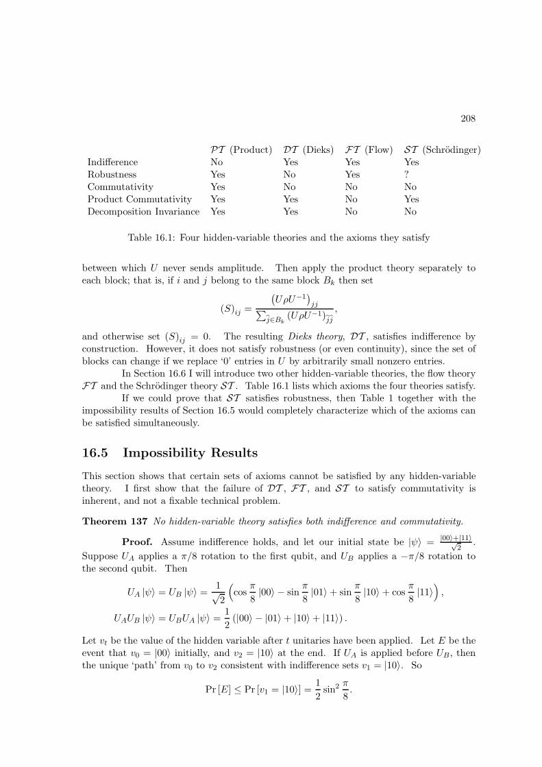
208

PT (Product) DT (Dieks) FT (Flow) ST (Schrodinger)Indifference No Yes Yes YesRobustness Yes No Yes ?Commutativity Yes No No NoProduct Commutativity Yes Yes No YesDecomposition Invariance Yes Yes No No

Table 16.1: Four hidden-variable theories and the axioms they satisfy

between which U never sends amplitude. Then apply the product theory separately toeach block; that is, if i and j belong to the same block Bk then set

(S)ij =

(UρU−1

)jj∑

j∈Bk(UρU−1)jj

,

and otherwise set (S)ij = 0. The resulting Dieks theory, DT , satisfies indifference byconstruction. However, it does not satisfy robustness (or even continuity), since the set ofblocks can change if we replace ‘0’ entries in U by arbitrarily small nonzero entries.

In Section 16.6 I will introduce two other hidden-variable theories, the flow theoryFT and the Schrodinger theory ST . Table 16.1 lists which axioms the four theories satisfy.

If we could prove that ST satisfies robustness, then Table 1 together with theimpossibility results of Section 16.5 would completely characterize which of the axioms canbe satisfied simultaneously.

16.5 Impossibility Results

This section shows that certain sets of axioms cannot be satisfied by any hidden-variabletheory. I first show that the failure of DT , FT , and ST to satisfy commutativity isinherent, and not a fixable technical problem.

Theorem 137 No hidden-variable theory satisfies both indifference and commutativity.

Proof. Assume indifference holds, and let our initial state be |ψ〉 = |00〉+|11〉√2

.

Suppose UA applies a π/8 rotation to the first qubit, and UB applies a −π/8 rotation tothe second qubit. Then

UA |ψ〉 = UB |ψ〉 =1√2

(cos

π

8|00〉 − sin

π

8|01〉 + sin

π

8|10〉 + cos

π

8|11〉

),

UAUB |ψ〉 = UBUA |ψ〉 =1

2(|00〉 − |01〉 + |10〉 + |11〉) .

Let vt be the value of the hidden variable after t unitaries have been applied. Let E be theevent that v0 = |00〉 initially, and v2 = |10〉 at the end. If UA is applied before UB , thenthe unique ‘path’ from v0 to v2 consistent with indifference sets v1 = |10〉. So

Pr [E] ≤ Pr [v1 = |10〉] =1

2sin2 π

8.

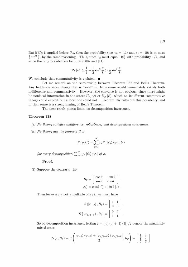
209

But if UB is applied before UA, then the probability that v0 = |11〉 and v2 = |10〉 is at most12 sin2 π

8 , by the same reasoning. Thus, since v2 must equal |10〉 with probability 1/4, andsince the only possibilities for v0 are |00〉 and |11〉,

Pr [E] ≥ 1

4− 1

2sin2 π

8>

1

2sin2 π

8.

We conclude that commutativity is violated.Let me remark on the relationship between Theorem 137 and Bell’s Theorem.

Any hidden-variable theory that is “local” in Bell’s sense would immediately satisfy bothindifference and commutativity. However, the converse is not obvious, since there mightbe nonlocal information in the states UA |ψ〉 or UB |ψ〉, which an indifferent commutativetheory could exploit but a local one could not. Theorem 137 rules out this possibility, andin that sense is a strengthening of Bell’s Theorem.

The next result places limits on decomposition invariance.

Theorem 138

(i) No theory satisfies indifference, robustness, and decomposition invariance.

(ii) No theory has the property that

P (ρ, U) =N∑

i=1

piP (|ψi〉〈ψi| , U)

for every decomposition∑N

i=1 pi |ψi〉〈ψi| of ρ.

Proof.

(i) Suppose the contrary. Let

Rθ =

[cos θ − sin θsin θ cos θ

],

|ϕθ〉 = cos θ |0〉 + sin θ |1〉 .

Then for every θ not a multiple of π/2, we must have

S (|ϕ−θ〉 , Rθ) =

[1 10 0

],

S(∣∣ϕπ/2−θ

⟩, Rθ

)=

[0 01 1

].

So by decomposition invariance, letting I = (|0〉〈0| + |1〉〈1|) /2 denote the maximallymixed state,

S (I,Rθ) = S

(|ϕ−θ〉〈ϕ−θ| +

∣∣ϕπ/2−θ⟩ ⟨ϕπ/2−θ

∣∣2

, Rθ

)=

[12

12

12

12

]

210

and therefore

P (I,Rθ) =

[(ρ)00

2(ρ)11

2(ρ)00

2(ρ)11

2

]=

[14

14

14

14

].

By robustness, this holds for θ = 0 as well. But this is a contradiction, since byindifference P (I,R0) must be half the identity.

(ii) Suppose the contrary; then

P(I,Rπ/8

)=P(|0〉 , Rπ/8

)+ P

(|1〉 , Rπ/8

)

2.

So considering transitions from |0〉 to |1〉,

(P(I,Rπ/8

))01

=

(P(|0〉 , Rπ/8

))11

+ 0

2=

1

2sin2 π

8.

But

P(I,Rπ/8

)=P(∣∣ϕπ/8

⟩, Rπ/8

)+ P

(∣∣ϕ5π/8

⟩, Rπ/8

)

2

also. Since Rπ/8∣∣ϕπ/8

⟩=∣∣ϕπ/4

⟩, we have

(P(I,Rπ/8

))01

≥ 1

2

(P(∣∣ϕπ/8

⟩, Rπ/8

))01

≥ 1

2

(1

2−(P(∣∣ϕπ/8

⟩, Rπ/8

))11

)

≥ 1

2

(1

2− sin2 π

8

)

>1

2sin2 π

8

which is a contradiction.

Notice that all three conditions in Theorem 138, part (i) were essential—for PTsatisfies robustness and decomposition invariance, DT satisfies indifference and decomposi-tion invariance, and FT satisfies indifference and robustness.

The last impossibility result says that no hidden-variable theory satisfies bothindifference and “strong continuity,” in the sense that for all ε > 0 there exists δ > 0 suchthat ‖ρ− ρ‖ ≤ δ implies ‖S (ρ, U) − S (ρ, U)‖ ≤ ε. To see this, let

U =

1 0 00 1√

2− 1√

2

0 1√2

1√2

,

ρ =√

1 − 2δ2 |0〉 + δ |1〉 + δ |2〉 ,ρ =

√1 − 2δ2 |0〉 + δ |1〉 − δ |2〉 .

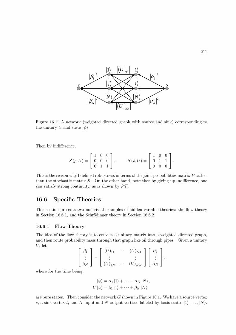
211

2

1α

2

Nα2

Nβ

2

1β

st

1

N

ij

1

N

( )11U

( )NNU

Figure 16.1: A network (weighted directed graph with source and sink) corresponding tothe unitary U and state |ψ〉

Then by indifference,

S (ρ, U) =

1 0 00 0 00 1 1

, S (ρ, U) =

1 0 00 1 10 0 0

.

This is the reason why I defined robustness in terms of the joint probabilities matrix P ratherthan the stochastic matrix S. On the other hand, note that by giving up indifference, onecan satisfy strong continuity, as is shown by PT .

16.6 Specific Theories

This section presents two nontrivial examples of hidden-variable theories: the flow theoryin Section 16.6.1, and the Schrodinger theory in Section 16.6.2.

16.6.1 Flow Theory

The idea of the flow theory is to convert a unitary matrix into a weighted directed graph,and then route probability mass through that graph like oil through pipes. Given a unitaryU , let

β1...βN

=

(U)11 · · · (U)N1...

...(U)1N · · · (U)NN

α1...αN

,

where for the time being

|ψ〉 = α1 |1〉 + · · · + αN |N〉 ,U |ψ〉 = β1 |1〉 + · · · + βN |N〉

are pure states. Then consider the network G shown in Figure 16.1. We have a source vertexs, a sink vertex t, and N input and N output vertices labeled by basis states |1〉 , . . . , |N〉.

212

Each edge of the form (s, |i〉) has capacity |αi|2, each edge (|i〉 , |j〉) has capacity∣∣∣(U)ij

∣∣∣,and each edge (|j〉 , t) has capacity |βj |2. A natural question is how much probability masscan flow from s to t without violating the capacity constraints. Rather surprisingly, I willshow that one unit of mass (that is, all of it) can. Interestingly, this result would be false

if edge (|i〉 , |j〉) had capacity∣∣∣(U)ij

∣∣∣2

(or even∣∣∣(U)ij

∣∣∣1+ε

) instead of∣∣∣(U)ij

∣∣∣. I will also

show that there exists a mapping from networks to maximal flows in those networks, thatis robust in the sense that a small change in edge capacities produces only a small changein the amount of flow through any edge.

The proofs of these theorems use classical results from the theory of network flows(see [88] for an introduction). In particular, let a cut be a set of edges that separates s fromt; the value of a cut is the sum of the capacities of its edges. Then a fundamental resultcalled the Max-Flow-Min-Cut Theorem [113] says that the maximum possible amount offlow from s to t equals the minimum value of any cut. Using that result I can show thefollowing.

Theorem 139 One unit of flow can be routed from s to t in G.

Proof. By the above, it suffices to show that any cut C in G has value at least 1.Let A be the set of i ∈ 1, . . . , N such that (s, |i〉) /∈ C, and let B be the set of j such that(|j〉 , t) /∈ C. Then C must contain every edge (|i〉 , |j〉) such that i ∈ A and j ∈ B, and wecan assume without loss of generality that C contains no other edges. So the value of C is

∑

i/∈A|αi|2 +

∑

j /∈B|βj |2 +

∑

i∈A, j∈B

∣∣∣(U)ij

∣∣∣ .

Therefore we need to prove the matrix inequality

(1 −

∑

i∈A|αi|2

)+

1 −

∑

j∈B|βj |2

+

∑

i∈A, j∈B

∣∣∣(U)ij

∣∣∣ ≥ 1,

or1 +

∑

i∈A, j∈B

∣∣∣(U)ij

∣∣∣ ≥∑

i∈A|αi|2 +

∑

j∈B|βj |2 . (16.1)

Let U be fixed, and consider the maximum of the right-hand side of equation (16.1) overall |ψ〉. Since

βj =∑

i

(U)ij αi,

this maximum is equal to the largest eigenvalue λ of the positive semidefinite matrix

∑

i∈A|i〉〈i| +

∑

j∈B|uj〉〈uj|

where for each j,|uj〉 = (U)1j |1〉 + · · · + (U)Nj |N〉 .

213

Let HA be the subspace of states spanned by |i〉 : i ∈ A, and let HB be the subspacespanned by |uj〉 : j ∈ B. Also, let LA (|ψ〉) be the length of the projection of |ψ〉 ontoHA, and let LB (|ψ〉) be the length of the projection of |ψ〉 onto HB . Then since the |i〉’sand |uj〉’s form orthogonal bases for HA and HB respectively, we have

λ = max|ψ〉

∑

i∈A|〈i|ψ〉|2 +

∑

j∈B|〈uj|ψ〉|2

= max|ψ〉

(LA (|ψ〉)2 + LB (|ψ〉)2

).

So letting θ be the angle between HA and HB,

λ = 2cos2 θ

2= 1 + cos θ

≤ 1 + max|a〉∈HA, |b〉∈HB

|〈a|b〉|

= 1 + max|γ1|2+···+|γN |2=1

|δ1|2+···+|δN |2=1

∣∣∣∣∣∣

(∑

i∈Aγi 〈i|

)∑

j∈Bδj |uj〉

∣∣∣∣∣∣

≤ 1 +∑

i∈A, j∈B

∣∣∣(U)ij

∣∣∣

which completes the theorem.Observe that Theorem 139 still holds if U acts on a mixed state ρ, since we

can write ρ as a convex combination of pure states |ψ〉〈ψ|, construct a flow for each |ψ〉separately, and then take a convex combination of the flows.

Using Theorem 139, I now define the flow theory FT . Let F (ρ, U) be the setof maximal flows for ρ, U—representable by N × N arrays of real numbers fij such that

0 ≤ fij ≤∣∣∣(U)ij

∣∣∣ for all i, j, and also

∑

j

fij = (ρ)ii ,∑

i

fij =(UρU−1

)jj.

Clearly F (ρ, U) is a convex polytope, which Theorem 139 asserts is nonempty. Form amaximal flow f∗ (ρ, U) ∈ F (ρ, U) as follows: first let f∗11 be the maximum of f11 overall f ∈ F (ρ, U). Then let f∗12 be the maximum of f12 over all f ∈ F (ρ, U) such thatf11 = f∗11. Continue to loop through all i, j pairs in lexicographic order, setting each f∗ij toits maximum possible value consistent with the (i− 1)N + j − 1 previous values. Finally,let (P )ij = f∗ij for all i, j. As discussed in Section 16.3, given P we can easily obtain the

stochastic matrix S by dividing the ith column by (ρ)ii, or taking a limit in case (ρ)ii = 0.It is easy to check that FT so defined satisfies the indifference axiom. Showing

that FT satisfies robustness is harder. Our proof is based on the Ford-Fulkerson algorithm[113], a classic algorithm for computing maximal flows that works by finding a sequence of“augmenting paths,” each of which increases the flow from s to t by some positive amount.

214

Theorem 140 FT satisfies robustness.

Proof. Let G be an arbitrary flow network with source s, sink t, and directededges e1, . . . , em, where each ei has capacity ci and leads from vi to wi. It will be convenientto introduce a fictitious edge e0 from t to s with unlimited capacity; then maximizing theflow through G is equivalent to maximizing the flow through e0. Suppose we produce anew network G by increasing a single capacity ci∗ by some ε > 0. Let f∗ be the optimalflow for G, obtained by first maximizing the flow f0 through e0, then maximizing the flowf1 through e1 holding f0 fixed, and so on up to fm. Let f∗ be the maximal flow for Gproduced in the same way. We claim that for all i ∈ 0, . . . ,m,

∣∣∣f∗i − f∗i∣∣∣ ≤ ε.

To see that the theorem follows from this claim: first, if f∗ is robust under adding ε toci∗ , then it must also be robust under subtracting ε from ci∗ . Second, if we change ρ, U

to ρ, U such that ‖ρ− ρ‖∞ ≤ 1/q (N) and∥∥∥U − U

∥∥∥∞

≤ 1/q (N), then we can imagine the

N2 + 2N edge capacities are changed one by one, so that

∥∥∥f∗(ρ, U

)− f∗ (ρ, U)

∥∥∥∞

≤∑

ij

∣∣∣∣∣∣∣∣(U)ij

∣∣∣∣−∣∣∣(U)ij

∣∣∣∣∣∣∣+∑

i

|(ρ)ii − (ρ)ii|

+∑

j

∣∣∣∣(U ρU−1

)jj−(UρU−1

)jj

∣∣∣∣

≤ 4N2

q (N).

(Here we have made no attempt to optimize the bound.)We now prove the claim. To do so we describe an iterative algorithm for computing

f∗. First maximize the flow f0 through e0, by using the Ford-Fulkerson algorithm to finda maximal flow from s to t. Let f (0) be the resulting flow, and let G(1) be the residualnetwork that corresponds to f (0). For each i, that is, G(1) has an edge ei = (vi, wi) of

capacity c(1)i = ci − f

(0)i , and an edge ei = (wi, vi) of capacity c

(1)i = f

(0)i . Next maximize

f1 subject to f0 by using the Ford-Fulkerson algorithm to find “augmenting cycles” fromw1 to v1 and back to w1 in G(1) \e0, e0. Continue in this manner until each of f1, . . . , fmhas been maximized subject to the previous fi’s. Finally set f∗ = f (m).

Now, one way to compute f∗ is to start with f∗, then repeatedly “correct” itby applying the same iterative algorithm to maximize f0, then f1, and so on. Let εi =∣∣∣f∗i − f∗i

∣∣∣; then we need to show that εi ≤ ε for all i ∈ 0, . . . ,m. The proof is by induction

on i. Clearly ε0 ≤ ε, since increasing ci∗ by ε can increase the value of the minimum cutfrom s to t by at most ε. Likewise, after we maximize f0, the value of the minimum cutfrom w1 to v1 can increase by at most ε−ε0 +ε0 = ε. For of the at most ε new units of flowfrom w1 to v1 that increasing ci∗ made available, ε0 of them were “taken up” in maximizingf0, but the process of maximizing f0 could have again increased the minimum cut from w1

to v1 by up to ε0. Continuing in this way,

ε2 ≤ ε− ε0 + ε0 − ε1 + ε1 = ε,

215

and so on up to εm. This completes the proof.That FT violates decomposition invariance now follows from Theorem 138, part

(i). One can also show that FT violates product commutativity, by considering the fol-lowing example: let |ψ〉 =

∣∣ϕπ/4⟩⊗∣∣ϕ−π/8

⟩be a 2-qubit initial state, and let RAπ/4 and RBπ/4

be π/4 rotations applied to the first and second qubits respectively. Then

S(RAπ/4 |ψ〉 , RBπ/4

)S(|ψ〉 , RAπ/4

)6= S

(RBπ/4 |ψ〉 , RAπ/4

)S(|ψ〉 , RBπ/4

).

We omit a proof for brevity.

16.6.2 Schrodinger Theory

The final hidden-variable theory, which I call the Schrodinger theory or ST , is the mostinteresting one mathematically. The idea—to make a matrix into a stochastic matrix viarow and column rescaling—is natural enough that we came upon it independently, only laterlearning that it originated in a 1931 paper of Schrodinger [215]. The idea was subsequentlydeveloped by Fortet [114], Beurling [58], Nagasawa [181], and others. My goal is to givewhat (to my knowledge) is the first self-contained, reasonably accessible presentation of themain result in this area; and to interpret that result in what I think is the correct way: asproviding one example of a hidden-variable theory, whose strengths and weaknesses shouldbe directly compared to those of other theories.

Most of the technical difficulties in [58, 114, 181, 215] arise because the stochasticprocess being constructed involves continuous time and particle positions. Here I eliminatethose difficulties by restricting attention to discrete time and finite-dimensional Hilbertspaces. I thereby obtain a generalized version5 of a problem that computer scientists knowas (r, c)-scaling of matrices [223, 120, 169].

As in the case of the flow theory, given a unitary U acting on a state ρ, the firststep is to replace each entry of U by its absolute value, obtaining a nonnegative matrix

U (0) defined by(U (0)

)ij

:=∣∣∣(U)ij

∣∣∣. We then wish to find nonnegative column multipliers

α1, . . . , αN and row multipliers β1, . . . , βN such that for all i, j,

αiβ1

(U (0)

)i1

+ · · · + αiβN

(U (0)

)iN

= (ρ)ii , (16.2)

α1βj

(U (0)

)1j

+ · · · + αNβj

(U (0)

)Nj

=(UρU−1

)jj. (16.3)

If we like, we can interpret the αi’s and βj ’s as dynamical variables that reach equilibriumprecisely when equations (16.2) and (16.3) are satisfied. Admittedly, it might be thoughtphysically implausible that such a complicated dynamical process should take place at everyinstant of time. On the other hand, it is hard to imagine a more “benign” way to convertU (0) into a joint probabilities matrix, than by simply rescaling its rows and columns.

I will show that multipliers satisfying (16.2) and (16.3) always exist. The intuitionof a dynamical process reaching equilibrium turns out to be key to the proof. For all t ≥ 0,

5In (r, c)-scaling, we are given an invertible real matrix, and the goal is to rescale all rows and columnsto sum to 1. The generalized version is to rescale the rows and columns to given values (not necessarily 1).

216

let

(U (2t+1)

)ij

=(ρ)ii∑

k

(U (2t)

)ik

(U (2t)

)ij,

(U (2t+2)

)ij

=

(UρU−1

)jj∑

k

(U (2t+1)

)kj

(U (2t+1)

)ij.

In words, we obtain U (2t+1) by normalizing each column i of U (2t) to sum to (ρ)ii; likewisewe obtain U (2t+2) by normalizing each row j of U (2t+1) to sum to

(UρU−1

)jj

. The crucial

fact is that the above process always converges to some P (ρ, U) = limt→∞ U (t). We cantherefore take

αi =

∞∏

t=0

(ρ)ii∑k

(U (2t)

)ik

,

βj =

∞∏

t=0

(UρU−1

)jj∑

k

(U (2t+1)

)kj

for all i, j. Although I will not prove it here, it turns out that this yields the unique solutionto equations (16.2) and (16.3), up to a global rescaling of the form αi → αic for all i andβj → βj/c for all j [181].

The convergence proof will reuse a result about network flows from Section 16.6.1,in order to define a nondecreasing “progress measure” based on Kullback-Leibler distance.

Theorem 141 The limit P (ρ, U) = limt→∞ U (t) exists.

Proof. A consequence of Theorem 139 is that for every ρ, U , there exists an N×Narray of nonnegative real numbers fij such that

(1) fij = 0 whenever∣∣∣(U)ij

∣∣∣ = 0,

(2) fi1 + · · · + fiN = (ρ)ii for all i, and

(3) f1j + · · · + fNj =(UρU−1

)jj

for all j.

Given any such array, define a progress measure

Z(t) =∏

ij

(U (t)

)fij

ij,

where we adopt the convention 00 = 1. We claim that Z(t+1) ≥ Z(t) for all t ≥ 1. Tosee this, assume without loss of generality that we are on an odd step 2t + 1, and let

217

C(2t)i =

∑j

(U (2t)

)ij

be the ith column sum before we normalize it. Then

Z(2t+1) =∏

ij

(U (2t+1)

)fij

ij

=∏

ij

((ρ)ii

C(2t)i

(U (2t)

)ij

)fij

=

∏

ij

(U (2t)

)fij

ij

∏

i

((ρ)ii

C(2t)i

)fi1+···+fiN

= Z(2t) ·∏

i

((ρ)ii

C(2t)i

)(ρ)ii

.

As a result of the 2tth normalization step, we had∑

iC(2t)i = 1. Subject to that constraint,

the maximum of ∏

i

(C

(2t)i

)(ρ)ii

over the C(2t)i ’s occurs when C

(2t)i = (ρ)ii for all i—a simple calculus fact that follows

from the nonnegativity of Kullback-Leibler distance. This implies that Z(2t+1) ≥ Z(2t).Similarly, normalizing rows leads to Z(2t+2) ≥ Z(2t+1).

It follows that the limit P (ρ, U) = limt→∞ U (t) exists. For suppose not; then some

C(t)i is bounded away from (ρ)ii, so there exists an ε > 0 such that Z(t+1) ≥ (1 + ε)Z(t) for

all even t. But this is a contradiction, since Z(0) > 0 and Z(t) ≤ 1 for all t.Besides showing that P (ρ, U) is well-defined, Theorem 141 also yields a procedure

to calculate P (ρ, U) (as well as the αi’s and βj ’s). It can be shown that this procedureconverges to within entrywise error ε after a number steps polynomial in N and 1/ε. Also,once we have P (ρ, U), the stochastic matrix S (ρ, U) is readily obtained by normalizingeach column of P (ρ, U) to sum to 1. This completes the definition of the Schrodingertheory ST .

It is immediate that ST satisfies indifference. Also:

Proposition 142 ST satisfies product commutativity.

Proof. Given a state |ψ〉 = |ψA〉⊗|ψB〉, let UA⊗I act only on |ψA〉 and let I⊗UBact only on |ψB〉. Then we claim that

S (|ψ〉 , UA ⊗ I) = S (|ψA〉 , UA) ⊗ I.

The reason is simply that multiplying all amplitudes in |ψA〉 and UA |ψA〉 by a constantfactor αx, as we do for each basis state |x〉 of |ψB〉, has no effect on the scaling procedurethat produces S (|ψA〉 , UA). Similarly

S (|ψ〉 , I ⊗ UB) = I ⊗ S (|ψB〉 , UB) .

218

It follows that

S (|ψA〉 , UA) ⊗ S (|ψB〉 , UB) = S (UA |ψA〉 ⊗ |ψB〉 , I ⊗ UB)S (|ψ〉 , UA ⊗ I)

= S (|ψA〉 ⊗ UB |ψB〉 , UA ⊗ I)S (|ψ〉 , I ⊗ UB) .

On the other hand, numerical simulations readily show that ST violates decom-position invariance, even when N = 2 (I omit a concrete example for brevity).

16.7 The Computational Model

I now explain the histories model of computation, building up to the complexity class DQP.From now on, the states ρ that we consider will always be pure states of ` = log2N qubits.That is, ρ = |ψ〉〈ψ| where

|ψ〉 =∑

x∈0,1`

αx |x〉 .

The algorithms of this chapter will work under any hidden-variable theory thatsatisfies the indifference axiom. On the other hand, if we take into account that even intheory (let alone in practice), a generic unitary cannot be represented exactly with a finiteuniversal gate set, only approximated arbitrarily well, then we also need the robustnessaxiom. Thus, it is reassuring that there exists a hidden-variable theory (namely FT ) thatsatisfies both indifference and robustness.

Let a quantum computer have the initial state |0〉⊗`, and suppose we apply asequence U = (U1, . . . , UT ) of unitary operations, each of which is implemented by apolynomial-size quantum circuit. Then a history of a hidden variable through the com-putation is a sequence H = (v0, . . . , vT ) of basis states, where vt is the variable’s valueimmediately after Ut is applied (thus v0 = |0〉⊗`). Given any hidden-variable theory T , wecan obtain a probability distribution Ω (U ,T ) over histories by just applying T repeatedly,once for each Ut, to obtain the stochastic matrices

S(|0〉⊗` , U1

), S

(U1 |0〉⊗` , U2

), . . . S

(UT−1 · · ·U1 |0〉⊗` , UT

).

Note that Ω (U ,T ) is a Markov distribution; that is, each vt is independent of the other vi’sconditioned on vt−1 and vt+1. Admittedly, Ω (U ,T ) could depend on the precise way inwhich the combined circuit UT · · ·U1 is “sliced” into component circuits U1, . . . , UT . Butas noted in Section 16.3.2, such dependence on the granularity of unitaries is unavoidablein any hidden-variable theory other than PT .

Given a hidden-variable theory T , let O (T ) be an oracle that takes as input apositive integer `, and a sequence of quantum circuits U = (U1, . . . , UT ) that act on ` qubits.Here each Ut is specified by a sequence

(gt,1, . . . , gt,m(t)

)of gates chosen from some finite

universal gate set G. The oracle O (T ) returns as output a sample (v0, . . . , vT ) from thehistory distribution Ω (U ,T ) defined previously. Now let A be a deterministic classicalTuring machine that is given oracle access to O (T ). The machine A receives an input x,makes a single oracle query to O (T ), then produces an output based on the response. We

219

say a set of strings L is in DQP if there exists an A such that for all sufficiently large n andinputs x ∈ 0, 1n, and all theories T satisfying the indifference and robustness axioms, Acorrectly decides whether x ∈ L with probability at least 2/3, in time polynomial in n.

Let me make some remarks about the above definition. There is no real signifi-cance in the requirement that A be deterministic and classical, and that it be allowed onlyone query to O (T ). I made this choice only because it suffices for the upper bounds; itmight be interesting to consider the effects of other choices. However, other aspects of thedefinition are not arbitrary. The order of quantifiers matters; we want a single A that worksfor any hidden-variable theory satisfying indifference and robustness. Also, we require Ato succeed only for sufficiently large n since by choosing a large enough polynomial q (N)in the statement of the robustness axiom, an adversary might easily make A incorrect on afinite number of instances.

16.7.1 Basic Results

Having defined the complexity class DQP, in this subsection I establish its most basicproperties. First of all, it is immediate that BQP ⊆ DQP; that is, sampling histories is atleast as powerful as standard quantum computation. For v1, the first hidden-variable valuereturned by O (T ), can be seen as simply the result of applying a polynomial-size quantumcircuit U1 to the initial state |0〉⊗` and then measuring in the standard basis. A key furtherobservation is the following.

Theorem 143 Any universal gate set yields the same complexity class DQP. By universal,we mean that any unitary matrix (real or complex) can be approximated, without the needfor ancilla qubits.

Proof. Let G and G′ be universal gate sets. Also, let U = (U1, . . . , UT ) be asequence of `-qubit unitaries, each specified by a polynomial-size quantum circuit over G.We have T, ` = O (poly (n)) where n is the input length. We can also assume without lossof generality that ` ≥ n, since otherwise we simply insert n−` dummy qubits that are neveracted on (by the indifference axiom, this will not affect the results). We want to approximateU by another sequence of `-qubit unitaries, U ′ = (U ′

1, . . . , U′T ), where each U ′

t is specified

by a quantum circuit over G′. In particular, for all t we want ‖U ′t − Ut‖∞ ≤ 2−`

2T . Bythe Solovay-Kitaev Theorem [155, 184], we can achieve this using poly

(n, `2T

)= poly (n)

gates from G′; moreover, the circuit for U ′t can be constructed in polynomial time given the

circuit for Ut.Let |ψt〉 = Ut · · ·U1 |0〉⊗` and |ψ′

t〉 = U ′t · · ·U ′

1 |0〉⊗`. Notice that for all t ∈1, . . . , T,

∥∥∣∣ψ′t

⟩− |ψt〉

∥∥∞ ≤ 2`

(∥∥∣∣ψ′t−1

⟩− |ψt−1〉

∥∥∞ + 2−`

2T)

≤ T2`T(2−`

2T)

= T2−`(`−1)T ,

since ‖|ψ′0〉 − |ψ0〉‖∞ = 0. Here ‖ ‖∞ denotes the maximum entrywise difference between

two vectors in C2`. Also, given a theory T , let Pt and P ′

t be the joint probabilities matrices

220

corresponding to Ut and U ′t respectively. Then by the robustness axiom, there exists

a polynomial q such that if ‖U ′t − Ut‖∞ ≤ 1/q

(2`)

and∥∥∣∣ψ′

t−1

⟩− |ψt−1〉

∥∥∞ ≤ 1/q

(2`),

then ‖Pt − P ′t‖∞ ≤ 2−3`. For all such polynomials q, we have 2−`

2T ≤ 1/q(2`)

and

T2−`(`−1)T ≤ 1/q(2`)

for sufficiently large n ≤ `. Therefore ‖Pt − P ′t‖∞ ≤ 2−3` for all t

and sufficiently large n.Now assume n is sufficiently large, and consider the distributions Ω (U ,T ) and

Ω (U ′,T ) over classical histories H = (v0, . . . , vT ). For all t ∈ 1, . . . , T and x ∈ 0, 1`,we have ∣∣∣∣ Pr

Ω(U ,T )[vt = |x〉] − Pr

Ω(U ′,T )[vt = |x〉]

∣∣∣∣ ≤ 2`(2−3`

)= 2−2`.

It follows by the union bound that the variation distance ‖Ω (U ′,T ) − Ω (U ,T )‖ is at most

T2`(2−2`

)=T

2`≤ T

2n.

In other words, Ω (U ′,T ) can be distinguished from Ω (U ,T ) with bias at most T/2n, whichis exponentially small. So any classical postprocessing algorithm that succeeds with highprobability given H ∈ Ω (U ,T ), also succeeds with high probability given H ∈ Ω (U ′,T ).This completes the theorem.

Unfortunately, the best upper bound on DQP I have been able to show is DQP ⊆EXP; that is, any problem in DQP is solvable in deterministic exponential time. The proofis trivial: let T be the flow theory FT . Then by using the Ford-Fulkerson algorithm, we canclearly construct the requisite maximum flows in time polynomial in 2` (hence exponentialin n), and thereby calculate the probability of each possible history (v1, . . . , vT ) to suitableprecision.

16.8 The Juggle Subroutine

This section presents a crucial subroutine that will be used in both main algorithms: thealgorithm for simulating statistical zero knowledge in Section 16.9, and the algorithm forsearch in N1/3 queries in Section 16.10. Given an `-qubit state (|a〉 + |b〉) /

√2, where |a〉

and |b〉 are unknown basis states, the goal of the juggle subroutine is to learn both a andb. The name arises because the strategy will be to “juggle” a hidden variable, so that ifit starts out at |a〉 then with non-negligible probability it transitions to |b〉, and vice versa.Inspecting the entire history of the hidden variable will then reveal both a and b, as desired.

To produce this behavior, we will exploit a basic feature of quantum mechanics:that observable information in one basis can become unobservable phase information in adifferent basis. We will apply a sequence of unitaries that hide all information about a andb in phases, thereby forcing the hidden variable to “forget” whether it started at |a〉 or |b〉.We will then invert those unitaries to return the state to (|a〉 + |b〉) /

√2, at which point the

hidden variable, having “forgotten” its initial value, must be unequal to that value withprobability 1/2.

I now give the subroutine. Let |ψ〉 = (|a〉 + |b〉) /√

2 be the initial state. Thefirst unitary, U1, consists of Hadamard gates on `− 1 qubits chosen uniformly at random,and the identity operation on the remaining qubit, i. Next U2 consists of a Hadamard gate

221

on qubit i. Finally U3 consists of Hadamard gates on all ` qubits. Let a = a1 . . . a` andb = b1 . . . b`. Then since a 6= b, we have ai 6= bi with probability at least 1/`. Assumingthat occurs, the state

U1 |ψ〉 =1

2`/2

∑

z∈0,1` : zi=ai

(−1)a·z−aizi |z〉 +∑

z∈0,1` : zi=bi

(−1)b·z−bizi |z〉

assigns nonzero amplitude to all 2` basis states. Then U2U1 |ψ〉 assigns nonzero amplitudeto 2`−1 basis states |z〉, namely those for which a·z ≡ b·z (mod 2). Finally U3U2U1 |ψ〉 = |ψ〉.

Let vt be the value of the hidden variable after Ut is applied. Then assumingai 6= bi, I claim that v3 is independent of v0. So in particular, if v0 = |a〉 then v3 = |b〉 with1/2 probability, and if v0 = |b〉 then v3 = |a〉 with 1/2 probability. To see this, observethat when U1 is applied, there is no interference between basis states |z〉 such that zi = ai,and those such that zi = bi. So by the indifference axiom, the probability mass at |a〉 mustspread out evenly among all 2`−1 basis states that agree with a on the ith bit, and similarlyfor the probability mass at |b〉. Then after U2 is applied, v2 can differ from v1 only on the ith

bit, again by the indifference axiom. So each basis state of U2U1 |ψ〉 must receive an equalcontribution from probability mass originating at |a〉, and probability mass originating at|b〉. Therefore v2 is independent of v0, from which it follows that v3 is independent of v0as well.

Unfortunately, the juggle subroutine only works with probability 1/ (2`)—for itrequires that ai 6= bi, and even then, inspecting the history (v0, v1, . . .) only reveals both|a〉 and |b〉 with probability 1/2. Furthermore, the definition of DQP does not allow morethan one call to the history oracle. However, all we need to do is pack multiple subroutinecalls into a single oracle call. That is, choose U4 similarly to U1 (except with a differentvalue of i), and set U5 = U2 and U6 = U3. Do the same with U7, U8, and U9, and soon. Since U3, U6, U9, . . . all return the quantum state to |ψ〉, the effect is that of multipleindependent juggle attempts. With 2`2 attempts, we can make the failure probability at

most (1 − 1/ (2`))2`2

< e−`.As a final remark, it is easy to see that the juggle subroutine works equally well

with states of the form |ψ〉 = (|a〉 − |b〉) /√

2. This will prove useful in Section 16.10.

16.9 Simulating SZK

This section shows that SZK ⊆ DQP. Here SZK, or Statistical Zero Knowledge, wasoriginally defined as the class of problems that possess a certain kind of “zero-knowledgeproof protocol”—that is, a protocol between an omniscient prover and a verifier, by whichthe verifier becomes convinced of the answer to a problem, yet without learning anythingelse about the problem. However, for present purposes this cryptographic definition ofSZK is irrelevant. For Sahai and Vadhan [211] have given an alternate and much simplercharacterization: a problem is in SZK if and only if it can be reduced to a problem calledStatistical Difference, which involves deciding whether two probability distributions areclose or far.

222

More formally, let P0 and P1 be functions that map n-bit strings to q (n)-bit stringsfor some polynomial q, and that are specified by classical polynomial-time algorithms. LetΛ0 and Λ1 be the probability distributions over P0 (x) and P1 (x) respectively, if x ∈ 0, 1nis chosen uniformly at random. Then the problem is to decide whether ‖Λ0 − Λ1‖ is lessthan 1/3 or greater than 2/3, given that one of these is the case. Here

‖Λ0 − Λ1‖ =1

2

∑

y∈0,1q(n)

∣∣∣∣ Prx∈0,1n

[P0 (x) = y] − Prx∈0,1n

[P1 (x) = y]

∣∣∣∣

is the variation distance between Λ0 and Λ1.To illustrate, let us see why Graph Isomorphism is in SZK. Given two graphs

G0 and G1, take Λ0 to be the uniform distribution over all permutations of G0, and Λ1 tobe uniform over all permutations of G1. This way, if G0 and G1 are isomorphic, then Λ0

and Λ1 will be identical, so ‖Λ0 − Λ1‖ = 0. On the other hand, if G0 and G1 are non-isomorphic, then Λ0 and Λ1 will be perfectly distinguishable, so ‖Λ0 − Λ1‖ = 1. Since Λ0

and Λ1 are clearly samplable by polynomial-time algorithms, it follows that any instanceof Graph Isomorphism can be expressed as an instance of Statistical Difference. For aproof that Approximate Shortest Vector is in SZK, the reader is referred to Goldreich andGoldwasser [131] (see also Aharonov and Ta-Shma [23]).

The proof will use the following “amplification lemma” from [211]:6

Lemma 144 (Sahai and Vadhan) Given efficiently-samplable distributions Λ0 and Λ1,we can construct new efficiently-samplable distributions Λ′

0 and Λ′1, such that if ‖Λ0 − Λ1‖ ≤

1/3 then ‖Λ′0 − Λ′

1‖ ≤ 2−n, while if ‖Λ0 − Λ1‖ ≥ 2/3 then ‖Λ′0 − Λ′

1‖ ≥ 1 − 2−n.

In particular, Lemma 144 means we can assume without loss of generality thateither ‖Λ0 − Λ1‖ ≤ 2−n

cor ‖Λ0 − Λ1‖ ≥ 1 − 2−n

cfor some constant c > 0.

Having covered the necessary facts about SZK, we can now proceed to the mainresult.

Theorem 145 SZK ⊆ DQP.

Proof. We show how to solve Statistical Difference by using a history oracle. Forsimplicity, we start with the special case where P0 and P1 are both one-to-one functions.In this case, the circuit sequence U given to the history oracle does the following: it firstprepares the state

1

2(n+1)/2

∑

b∈0,1,x∈0,1n

|b〉 |x〉 |Pb (x)〉 .

It then applies the juggle subroutine to the joint state of the |b〉 and |x〉 registers, taking` = n+ 1. Notice that by the indifference axiom, the hidden variable will never transitionfrom one value of Pb (x) to another—exactly as if we had measured the third register in thestandard basis. All that matters is the reduced state |ψ〉 of the first two registers, which

6Note that in this lemma, the constants 1/3 and 2/3 are not arbitrary; it is important for technicalreasons that (2/3)2 > 1/3.

223

has the form (|0〉 |x0〉 + |1〉 |x1〉) /√

2 for some x0, x1 if ‖Λ0 − Λ1‖ = 0, and |b〉 |x〉 for someb, x if ‖Λ0 − Λ1‖ = 1. We have already seen that the juggle subroutine can distinguishthese two cases: when the hidden-variable history is inspected, it will contain two values ofthe |b〉 register in the former case, and only one value in the latter case. Also, clearly thecase ‖Λ0 − Λ1‖ ≤ 2−n

cis statistically indistinguishable from ‖Λ0 − Λ1‖ = 0 with respect to

the subroutine, and likewise ‖Λ0 − Λ1‖ ≥ 1−2−nc

is indistinguishable from ‖Λ0 − Λ1‖ = 1.We now consider the general case, where P0 and P1 need not be one-to-one. Our

strategy is to reduce to the one-to-one case, by using a well-known hashing technique ofValiant and Vazirani [233]. Let Dn,k be the uniform distribution over all affine functions

mapping 0, 1n to 0, 1k, where we identify those sets with the finite fields Fn2 and Fk2respectively. What Valiant and Vazirani showed is that, for all subsets A ⊆ 0, 1n suchthat 2k−2 ≤ |A| ≤ 2k−1, and all s ∈ 0, 1k,

Prh∈Dn,k

[∣∣A ∩ h−1 (s)∣∣ = 1

]≥ 1

8.

As a corollary, the expectation over h ∈ Dn,k of

∣∣∣s ∈ 0, 1k :

∣∣A ∩ h−1 (s)∣∣ = 1

∣∣∣

is at least 2k/8. It follows that, if x is drawn uniformly at random from A, then

Prh,x

[∣∣A ∩ h−1 (h (x))∣∣ = 1

]≥ 2k/8

|A| ≥ 1

4.

This immediately suggests the following algorithm for the many-to-one case. Draw kuniformly at random from 2, . . . , n+ 1; then draw h0, h1 ∈ Dn,k. Have U prepare thestate

1

2(n+1)/2

∑

b∈0,1,x∈0,1n

|b〉 |x〉 |Pb (x)〉 |hb (x)〉 ,

and then apply the juggle subroutine to the joint state of the |b〉 and |x〉 registers, ignoringthe |Pb (x)〉 and |hb (x)〉 registers as before.

Suppose ‖Λ0 − Λ1‖ = 0. Also, given x ∈ 0, 1n and i ∈ 0, 1, let Ai =P−1i (Pi (x)) and Hi = h−1

i (hi (x)), and suppose 2k−2 ≤ |A0| = |A1| ≤ 2k−1. Then

Prs,h0,h1

[|A0 ∩H0| = 1 ∧ |A1 ∩H1| = 1] ≥(

1

4

)2

,

since the events |A0 ∩H0| = 1 and |A1 ∩H1| = 1 are independent of each other conditionedon x. Assuming both events occur, as before the juggle subroutine will reveal both |0〉 |x0〉and |1〉 |x1〉 with high probability, where x0 and x1 are the unique elements of A0 ∩ H0

and A1 ∩ H1 respectively. By contrast, if ‖Λ0 − Λ1‖ = 1 then only one value of the |b〉register will ever be observed. Again, replacing ‖Λ0 − Λ1‖ = 0 by ‖Λ0 − Λ1‖ ≤ 2−n

c, and

‖Λ0 − Λ1‖ = 1 by ‖Λ0 − Λ1‖ ≥ 1 − 2−nc, can have only a negligible effect on the history

distribution.

224

Of course, the probability that the correct value of k is chosen, and that A0 ∩H0

and A1 ∩H1 both have a unique element, could be as low as 1/ (16n). To deal with this,we simply increase the number of calls to the juggle subroutine by an O (n) factor, drawingnew values of k, h0, h1 for each call. We pack multiple subroutine calls into a single oraclecall as described in Section 16.8, except that now we uncompute the entire state (returningit to |0 · · · 0〉) and then recompute it between subroutine calls. A final remark: since thealgorithm that calls the history oracle is deterministic, we “draw” new values of k, h0, h1 byhaving U prepare a uniform superposition over all possible values. The indifference axiomjustifies this procedure, by guaranteeing that within each call to the juggle subroutine, thehidden-variable values of k, h0, and h1 remain constant.

Recall from Chapter 6 that there exists an oracle A relative to which SZKA 6∈BQPA. By contrast, since Theorem 145 is easily seen to relativize, we have SZKA ∈ DQPA

for all oracles A. It follows that there exists an oracle A relative to which BQPA 6= DQPA.

16.10 Search in N1/3 Queries

Given a Boolean function f : 0, 1n → 0, 1, the database search problem is simply tofind a string x such that f (x) = 1. We can assume without loss of generality that this“marked item” x is unique.7 We want to find it using as few queries to f as possible, wherea query returns f (y) given y.

LetN = 2n. Then classically, of course, Θ (N) queries are necessary and sufficient.By querying f in superposition, Grover’s algorithm [141] finds x using O

(N1/2

)queries,

together with O(N1/2

)auxiliary computation steps (here the O hides a factor of the form

(logN)c). Bennett et al. [51] showed that any quantum algorithm needs Ω(N1/2

)queries.

In this section, I show how to find the marked item by sampling histories, usingonly O

(N1/3

)queries and O

(N1/3

)computation steps. Formally, the model is as follows.

Each of the quantum circuits U1, . . . , UT that algorithm A gives to the history oracle O (T )is now able to query f . Suppose Ut makes qt queries to f ; then the total number of queriesmade by A is defined to be Q = q1 + · · · + qT . The total number of computation steps isat least the number of steps required to write down U1, . . . , UT , but could be greater.

Theorem 146 In the DQP model, we can search a database of N items for a unique markeditem using O

(N1/3

)queries and O

(N1/3

)computation steps.

Proof. Assume without loss of generality that N = 2n with n|3, and that eachdatabase item is labeled by an n-bit string. Let x ∈ 0, 1n be the label of the uniquemarked item. Then the sequence of quantum circuits U does the following: it first runsO(2n/3

)iterations of Grover’s algorithm, in order to produce the n-qubit state α |x〉 +

β∑

y∈0,1n |y〉, where

α =

√1

2n/3 + 2−n/3+1 + 1,

β = 2−n/3α

7For if there are multiple marked items, then we can reduce to the unique marked item case by using theValiant-Vazirani hashing technique described in Theorem 145.

225

(one can check that this state is normalized). Next U applies Hadamard gates to the firstn/3 qubits. This yields the state

2−n/6α∑

y∈0,1n/3

(−1)xA·y |y〉 |xB〉 + 2n/6β∑

z∈0,12n/3

|0〉⊗n/3 |z〉 ,

where xA consists of the first n/3 bits of x, and xB consists of the remaining 2n/3 bits. LetY be the set of 2n/3 basis states of the form |y〉 |xB〉, and Z be the set of 22n/3 basis states

of the form |0〉⊗n/3 |z〉.Notice that 2−n/6α = 2n/6β. So with the sole exception of |0〉⊗n/3 |xB〉 (which

belongs to both Y and Z), the “marked” basis states in Y have the same amplitude as the“unmarked” basis states in Z. This is what we wanted. Notice also that, if we manage tofind any |y〉 |xB〉 ∈ Y , then we can find x itself using 2n/3 further classical queries: simplytest all possible strings that end in xB. Thus, the goal of our algorithm will be to cause thehidden variable to visit an element of Y , so that inspecting the variable’s history revealsthat element.

As in Theorem 145, the tools that we need are the juggle subroutine, and a wayof reducing many basis states to two. Let s be drawn uniformly at random from 0, 1n/3.Then U appends a third register to the state, and sets it equal to |z〉 if the first two registers

have the form |0〉⊗n/3 |z〉, or to |s, y〉 if they have the form |y〉 |xB〉. Disregarding the basis

state |0〉⊗n/3 |xB〉 for convenience, the result is

2−n/6α

∑

y∈0,1n/3

(−1)xA·y |y〉 |xB〉 |s, y〉 +∑

z∈0,12n/3

|0〉⊗n/3 |z〉 |z〉

.

Next U applies the juggle subroutine to the joint state of the first two registers. Supposethe hidden-variable value has the form |0〉⊗n/3 |z〉 |z〉 (that is, lies outside Y ). Then withprobability 2−n/3 over s, the first n/3 bits of z are equal to s. Suppose this event occurs.Then conditioned on the third register being |z〉, the reduced state of the first two registersis

(−1)xA·zB |zB〉 |xB〉 + |0〉⊗n/3 |z〉√2

,

where zB consists of the last n/3 bits of z. So it follows from Section 16.8 that withprobability Ω (1/n), the juggle subroutine will cause the hidden variable to transition from

|0〉⊗n/3 |z〉 to |zB〉 |xB〉, and hence from Z to Y .The algorithm calls the juggle subroutine Θ

(2n/3n

)= Θ

(N1/3 logN

)times, draw-

ing a new value of s and recomputing the third register after each call. Each call movesthe hidden variable from Z to Y with independent probability Ω

(2−n/3/n

); therefore with

high probability some call does so. Note that this juggling phase does not involve anydatabase queries. Also, as in Theorem 145, “drawing” s really means preparing a uniformsuperposition over all possible s. Finally, the probability that the hidden variable ever vis-its the basis state |0〉⊗n/3 |xB〉 is exponentially small (by the union bound), which justifiesour having disregarded it.

226

A curious feature of Theorem 146 is the tradeoff between queries and computationsteps. Suppose we had run Q iterations of Grover’s algorithm, or in other words made Qqueries to f . Then provided Q ≤

√N , the marked state |x〉 would have occurred with

probability Ω(Q2/N

), meaning that O

(N/Q2

)calls to the juggle subroutine would have

been sufficient to find x. Of course, the choice of Q that minimizes maxQ,N/Q2

is

Q = N1/3. On the other hand, had we been willing to spend O (N) computation steps, wecould have found x with only a single query!8 Thus, one might wonder whether some otheralgorithm could push the number of queries below N1/3, without simultaneously increasingthe number of computation steps. The following theorem rules out that possibility.

Theorem 147 In the DQP model, Ω(N1/3

)computation steps are needed to search an N -

item database for a unique marked item. As a consequence, there exists an oracle relativeto which NP 6⊂ DQP; that is, NP-complete problems are not efficiently solvable by samplinghistories.

Proof. Let N = 2n and f : 0, 1n → 0, 1. Given a sequence of quantumcircuits U = (U1, . . . , UT ) that query f , and assuming that x ∈ 0, 1n is the unique stringsuch that f (x) = 1, let |ψt (x)〉 be the quantum state after Ut is applied but before Ut+1

is. Then the “hybrid argument” of Bennett et al. [51] implies that, by simply changing thelocation of the marked item from x to x∗, we can ensure that

‖|ψt (x)〉 − |ψt (x∗)〉‖ = O

(Q2t

N

)

where ‖ ‖ represents trace distance, and Qt is the total number of queries made to f byU1, . . . , Ut. Therefore O

(Q2t /N

)provides an upper bound on the probability of noticing

the x→ x∗ change by monitoring vt, the value of the hidden variable after Ut is applied. Soby the union bound, the probability of noticing the change by monitoring the entire history(v1, . . . , vT ) is at most of order

T∑

t=1

Q2t

N≤ TQ2

T

N.

This cannot be Ω (1) unless T = Ω(N1/3

)or QT = Ω

(N1/3

), either of which implies an

Ω(N1/3

)lower bound on the total number of steps.To obtain an oracle relative to which NP 6⊂ DQP, we can now use a standard and

well-known “diagonalization method” due to Baker, Gill, and Solovay [41] to construct aninfinite sequence of exponentially hard search problems, such that any DQP machine failson at least one of the problems, whereas there exists an NP machine that succeeds on all ofthem. Details are omitted.

16.11 Conclusions and Open Problems

The idea that certain observables in quantum mechanics might have trajectories governedby dynamical laws has reappeared many times: in Schrodinger’s 1931 stochastic approach

8One should not make too much of this fact; one way to interpret it is simply that the “number of queries”should be redefined as Q+ T rather than Q.

227

[215], Bohmian mechanics [59], modal interpretations [39, 98, 99], and elsewhere. Yetbecause all of these proposals yield the same predictions for single-time probabilities, if weare to decide between them it must be on the basis of internal mathematical considerations.One message of this chapter has been that such considerations can actually get us quite far.

To focus attention on the core issues, I restricted attention to the simplest possiblesetting: discrete time, a finite-dimensional Hilbert space, and a single orthogonal basis.Within this setting, I proposed what seem like reasonable axioms that any hidden-variabletheory should satisfy: for example, indifference to the identity operation, robustness tosmall perturbations, and independence of the temporal order of spacelike-separated events.I then showed that not all of these axioms can be satisfied simultaneously. But perhaps moresurprisingly, I also showed that certain subsets of axioms can be satisfied for quite nontrivialreasons. In showing that the indifference and robustness axioms can be simultaneouslysatisfied, Section 16.6 revealed an unexpected connection between unitary matrices and theclassical theory of network flows.

As mentioned previously, an important open problem is to show that the Schrodingertheory satisfies robustness. Currently, I can only show that the matrix PST (ρ, U) is robustto exponentially small perturbations, not polynomially small ones. The problem is that ifany row or column sum in the U (t) matrix is extremely small, then the (r, c)-scaling processwill magnify tiny errors in the entries. Intuitively, though, this effect should be washed outby later scaling steps.

A second open problem is whether there exists a theory that satisfies indifference,as well as commutativity for all separable mixed states (not just separable pure states).A third problem is to investigate other notions of robustness—for example, robustness tosmall multiplicative rather than additive errors.

On the complexity side, perhaps the most interesting problem left open by thischapter is the computational complexity of simulating Bohmian mechanics. I stronglyconjecture that this problem, like the hidden-variable problems we have seen, is strictlyharder than simulating an ordinary quantum computer. The trouble is that Bohmianmechanics does not quite fit in the framework of this chapter: as discussed in Section16.3.2, we cannot have deterministic hidden-variable trajectories for discrete degrees offreedom such as qubits. Even worse, Bohmian mechanics violates the continuous analogueof the indifference axiom. On the other hand, this means that by trying to implement(say) the juggle subroutine with Bohmian trajectories, one might learn not only aboutBohmian mechanics and its relation to quantum computation, but also about how essentialthe indifference axiom really is for our implementation.

Another key open problem is to show better upper bounds on DQP. Recall thatI was only able to show DQP ⊆ EXP, by giving a classical exponential-time algorithm tosimulate the flow theory FT . Can we improve this to (say) DQP ⊆ PSPACE? Clearlyit would suffice to give a PSPACE algorithm that computes the transition probabilities forsome theory T satisfying the indifference and robustness axioms. On the other hand, thismight not be necessary—that is, there might be an indirect simulation method that doesnot work by computing (or even sampling from) the distribution over histories. It wouldalso be nice to pin down the complexities of simulating specific hidden-variable theories,such as FT and ST .

228

Chapter 17

Summary of Part II

Recall our hypothetical visitor from Conway’s Game of Life, on a complexity safariof the physical universe. Based on the results in Part II, the following are some intuitionsabout efficient computation that I would advise our visitor to toss in the garbage.

• We can be fairly confident that the class of functions efficiently computable in thephysical world coincides with P (or BPP, which is presumably equal).

• Although there are models of efficient computation more powerful than P, involvingthe manipulation of arbitrary real or complex numbers, these models will inevitablyblow up small errors in the numbers nonlinearly, and must be therefore be unphysical.

• A robot, moving at unit speed, would need order n steps to search a spatial region ofsize n for a marked item.

• The ability to see one’s entire “history” in a single time step cannot yield any complexity-theoretic advantage, since one could always just record the history as one went along,at the cost of a polynomial increase in memory.

On the other hand, just as in Part I, we have seen that many of the intuitions inour visitor’s suitcase are good to go. For example:

• If the items in a database have distance d from one another, then the time needed tosearch the database is about d times what it would be if the items had unit distancefrom one another.

• It is possible to choose a probability distribution over histories, in such a way that statei is never followed in a history by state j if the corresponding transition probabilityis zero, and such that a small change to the transition matrices produces only a smallchange in the history distribution.

• If, at the moment of your death, your entire life’s history flashed before you in aninstant, then you could probably still not solve NP-complete problems in polynomialtime.

229

Bibliography

[1] S. Aaronson. Book review on A New Kind of Science. Quantum Information andComputation, 2(5):410–423, 2002. quant-ph/0206089.

[2] S. Aaronson. Quantum lower bound for the collision problem. In Proc. ACM STOC,pages 635–642, 2002. quant-ph/0111102.

[3] S. Aaronson. Algorithms for Boolean function query properties. SIAM J. Comput.,32(5):1140–1157, 2003.

[4] S. Aaronson. Quantum certificate complexity. In Proc. IEEE Conference on Compu-tational Complexity, pages 171–178, 2003. ECCC TR03-005, quant-ph/0210020.

[5] S. Aaronson. Quantum lower bound for recursive Fourier sampling. Quantum Infor-mation and Computation, 3(2):165–174, 2003. ECCC TR02-072, quant-ph/0209060.

[6] S. Aaronson. The complexity of agreement. ECCC TR04-061, 2004.

[7] S. Aaronson. Is quantum mechanics an island in theoryspace? In A. Khrennikov,editor, Proceedings of the Vaxjo Conference “Quantum Theory: Reconsideration ofFoundations”, 2004. quant-ph/0401062.

[8] S. Aaronson. Limitations of quantum advice and one-way communication. Theory ofComputing, 2004. To appear. Conference version in Proc. IEEE Complexity 2004, pp.320-332. quant-ph/0402095.

[9] S. Aaronson. Lower bounds for local search by quantum arguments. In Proc. ACMSTOC, pages 465–474, 2004. ECCC TR03-057, quant-ph/0307149.

[10] S. Aaronson. Multilinear formulas and skepticism of quantum computing. In Proc.ACM STOC, pages 118–127, 2004. quant-ph/0311039.

[11] S. Aaronson. Quantum computing and hidden variables. Accepted to Phys. Rev. A.quant-ph/0408035 and quant-ph/0408119, 2004.

[12] S. Aaronson. NP-complete problems and physical reality: a survey. In preparation;invited for SIGACT News, 2005.

[13] S. Aaronson and A. Ambainis. Quantum search of spatial regions. Theory of Com-puting, 2004. To appear. Conference version in Proc. IEEE FOCS 2003, pp. 200-209.quant-ph/0303041.

230

[14] S. Aaronson and D. Gottesman. Improved simulation of stabilizer circuits. Phys. Rev.Lett., 70(052328), 2004. quant-ph/0406196.

[15] D. S. Abrams and S. Lloyd. Nonlinear quantum mechanics implies polynomial-timesolution for NP-complete and #P problems. Phys. Rev. Lett., 81:3992–3995, 1998.quant-ph/9801041.

[16] L. Adleman, J. DeMarrais, and M.-D. Huang. Quantum computability. SIAM J.Comput., 26(5):1524–1540, 1997.

[17] M. Agrawal, N. Kayal, and N. Saxena. PRIMES is in P.www.cse.iitk.ac.in/users/manindra/primality.ps, 2002.

[18] D. Aharonov. Quantum computation - a review. In Dietrich Stauffer, editor, AnnualReview of Computational Physics, volume VI. 1998. quant-ph/9812037.

[19] D. Aharonov, A. Ambainis, J. Kempe, and U. Vazirani. Quantum walks on graphs.In Proc. ACM STOC, pages 50–59, 2001. quant-ph/0012090.

[20] D. Aharonov and M. Ben-Or. Fault-tolerant quantum computation with constanterror. In Proc. ACM STOC, pages 176–188, 1997. quant-ph/9906129.

[21] D. Aharonov and T. Naveh. Quantum NP - a survey. quant-ph/0210077, 2002.

[22] D. Aharonov and O. Regev. Lattice problems in NP intersect coNP. In Proc. IEEEFOCS, pages 362–371, 2004.

[23] D. Aharonov and A. Ta-Shma. Adiabatic quantum state generation and statisticalzero knowledge. In Proc. ACM STOC, pages 20–29, 2003. quant-ph/0301023.

[24] D. Aldous. Minimization algorithms and random walk on the d-cube. Annals ofProbability, 11(2):403–413, 1983.

[25] A. Ambainis. In preparation.

[26] A. Ambainis. A note on quantum black-box complexity of almost all Boolean func-tions. Inform. Proc. Lett., 71:5–7, 1999. quant-ph/9811080.

[27] A. Ambainis. Quantum lower bounds by quantum arguments. J. Comput. Sys. Sci.,64:750–767, 2002. Earlier version in ACM STOC 2000. quant-ph/0002066.

[28] A. Ambainis. Polynomial degree vs. quantum query complexity. In Proc. IEEE FOCS,pages 230–239, 2003. quant-ph/0305028.

[29] A. Ambainis. Quantum lower bounds for collision and element distinctness with smallrange. quant-ph/0305179, 2003.

[30] A. Ambainis. Quantum walk algorithm for element distinctness. In Proc. IEEE FOCS,2004. quant-ph/0311001.

231

[31] A. Ambainis, J. Kempe, and A. Rivosh. Coins make quantum walks faster. InProc. ACM-SIAM Symp. on Discrete Algorithms (SODA), 2005. To appear. quant-ph/0402107.

[32] A. Ambainis, A. Nayak, A. Ta-Shma, and U. V. Vazirani. Quantum dense coding andquantum finite automata. J. ACM, 49:496–511, 2002. Earlier version in ACM STOC1999, pp. 376-383. quant-ph/9804043.

[33] A. Ambainis, L. J. Schulman, A. Ta-Shma, U. V. Vazirani, and A. Wigderson. Thequantum communication complexity of sampling. SIAM J. Comput., 32:1570–1585,2003.

[34] A. Ambainis, L. J. Schulman, and U. V. Vazirani. Computing with highly mixed states(extended abstract). In Proc. ACM STOC, pages 697–704, 2000. quant-ph/0003136.

[35] M. Arndt, O. Nairz, J. Vos-Andreae, C. Keller, G. van der Zouw, and A. Zeilinger.Wave-particle duality of C60 molecules. Nature, 401:680–682, 1999.

[36] S. Arora, R. Impagliazzo, and U. Vazirani. Relativizing versus nonrelativizing tech-niques: the role of local checkability. Manuscript, 1992.

[37] A. Aspect, P. Grangier, and G. Roger. Experimental realization of Einstein-Podolsky-Rosen-Bohm gedankenexperiment: a new violation of Bell’s inequalities. Phys. Rev.Lett., 49:91–94, 1982.

[38] L. Babai. Bounded round interactive proofs in finite groups. SIAM J. Discrete Math,5(1):88–111, 1992.

[39] G. Bacciagaluppi and M. Dickson. Dynamics for modal interpretations of quantumtheory. Found. Phys., 29:1165–1201, 1999. quant-ph/9711048.

[40] D. Bacon. Quantum computational complexity in the presence of closed timelikecurves. quant-ph/0309189, 2003.

[41] T. Baker, J. Gill, and R. Solovay. Relativizations of the P=?NP question. SIAM J.Comput., 4:431–442, 1975.

[42] S. Bakhtiari, R. Safavi-Naini, and J. Pieprzyk. Cryptographic hash functions: asurvey. Technical Report 95-09, Department of Computer Science, University of Wol-longong, July 1995.

[43] Z. Bar-Yossef, T. S. Jayram, and I. Kerenidis. Exponential separation of quantum andclassical one-way communication complexity. In Proc. ACM STOC, pages 128–137,2004. ECCC TR04-036.

[44] H. Barnum, M. Saks, and M. Szegedy. Quantum query complexity and semi-definiteprogramming. In Proc. IEEE Conference on Computational Complexity, pages 179–193, 2003.

232

[45] R. Beals, H. Buhrman, R. Cleve, M. Mosca, and R. de Wolf. Quantum lower boundsby polynomials. J. ACM, 48(4):778–797, 2001. Earlier version in IEEE FOCS 1998,pp. 352-361. quant-ph/9802049.

[46] R. Beigel. Perceptrons, PP, and the polynomial hierarchy. Computational Complexity,4:339–349, 1994.

[47] R. Beigel, N. Reingold, and D. Spielman. PP is closed under intersection. J. Comput.Sys. Sci., 50(2):191–202, 1995.

[48] J. D. Bekenstein. A universal upper bound on the entropy to energy ratio for boundedsystems. Phys. Rev. D, 23(2):287–298, 1981.

[49] J. S. Bell. Speakable and Unspeakable in Quantum Mechanics. Cambridge, 1987.

[50] P. Benioff. Space searches with a quantum robot. In S. J. Lomonaco and H. E. Brandt,editors, Quantum Computation and Information, Contemporary Mathematics Series.AMS, 2002. quant-ph/0003006.

[51] C. Bennett, E. Bernstein, G. Brassard, and U. Vazirani. Strengths and weaknesses ofquantum computing. SIAM J. Comput., 26(5):1510–1523, 1997. quant-ph/9701001.

[52] C. H. Bennett. Logical reversibility of computation. IBM Journal of Research andDevelopment, 17:525–532, 1973.

[53] C. H. Bennett, G. Brassard, C. Crepeau, R. Jozsa, A. Peres, and W. Wootters.Teleporting an unknown quantum state by dual classical and EPR channels. Phys.Rev. Lett., 70:1895–1898, 1993.

[54] C. H. Bennett and J. Gill. Relative to a random oracle A, PA 6= NPA 6= coNPA withprobability 1. SIAM J. Comput., 10(1):96–113, 1981.

[55] E. Bernstein and U. Vazirani. Quantum complexity theory. SIAM J. Comput.,26(5):1411–1473, 1997. First appeared in ACM STOC 1993.

[56] S. N. Bernstein. Sur l’ordre de la meilleure approximation des fonctions continuespar les polynomes de degre donne. Mem. Cl. Sci. Acad. Roy. Belg., 4:1–103, 1912.French.

[57] A. Berthiaume and G. Brassard. Oracle quantum computing. In Proc. Workshop onPhysics of Computation: PhysComp’92, pages 195–199. IEEE, 1992.

[58] A. Beurling. An automorphism of direct product measures. Ann. Math., 72:189–200,1960.

[59] D. Bohm. A suggested interpretation of the quantum theory in terms of “hidden”variables. Phys. Rev., 85:166–193, 1952.

[60] D. Bohm and B. Hiley. The Undivided Universe. Routledge, 1993.

233

[61] D. Boneh and R. Lipton. Algorithms for black box fields and their application tocryptography. In Proceedings of CRYPTO, volume 109, pages 283–297. Lecture Notesin Computer Science, 1996.

[62] M. L. Bonet and S. R. Buss. Size-depth tradeoff for Boolean formulae. Inform. Proc.Lett., 11:151–155, 1994.

[63] R. B. Boppana, J. Hastad, and S. Zachos. Does co-NP have short interactive proofs?Inform. Proc. Lett., 25:127–132, 1987.

[64] R. Bousso. Positive vacuum energy and the N-bound. J. High Energy Phys.,0011(038), 2000. hep-th/0010252.

[65] R. Bousso. The holographic principle. Reviews of Modern Physics, 74(3), 2002. hep-th/0203101.

[66] M. Boyer, G. Brassard, P. Høyer, and A. Tapp. Tight bounds on quantum searching.Fortschritte Der Physik, 46(4-5):493–505, 1998. quant-ph/9605034.

[67] G. Brassard, P. Høyer, M. Mosca, and A. Tapp. Quantum amplitude amplificationand estimation. In S. J. Lomonaco and H. E. Brandt, editors, Quantum Computationand Information, Contemporary Mathematics Series. AMS, 2002. quant-ph/0005055.

[68] G. Brassard, P. Høyer, and A. Tapp. Quantum algorithm for the collision problem.ACM SIGACT News, 28:14–19, 1997. quant-ph/9705002.

[69] S. L. Braunstein, C. M. Caves, N. Linden, S. Popescu, and R. Schack. Separability ofvery noisy mixed states and implications for NMR quantum computing. Phys. Rev.Lett., 83:1054–1057, 1999. quant-ph/9811018.

[70] R. P. Brent. The parallel evaluation of general arithmetic expressions. J. ACM,21:201–206, 1974.

[71] H. J. Briegel and R. Raussendorf. Persistent entanglement in arrays of interactingparticles. Phys. Rev. Lett., 86:910–913, 2001. quant-ph/0004051.

[72] T. Brun. Computers with closed timelike curves can solve hard problems. Foundationsof Physics Letters, 16:245–253, 2003. gr-qc/0209061.

[73] N. H. Bshouty, R. Cleve, and W. Eberly. Size-depth tradeoffs for algebraic formulae.SIAM J. Comput., 24(4):682–705, 1995.

[74] S. Bublitz, U. Schurfeld, B. Voigt, and I. Wegener. Properties of complexity measuresfor PRAMs and WRAMs. Theoretical Comput. Sci., 48:53–73, 1986.

[75] H. Buhrman, R. Cleve, J. Watrous, and R. de Wolf. Quantum fingerprinting. Phys.Rev. Lett., 87(16), 2001. quant-ph/0102001.

[76] H. Buhrman, R. Cleve, and A. Wigderson. Quantum vs. classical communication andcomputation. In Proc. ACM STOC, pages 63–68, 1998. quant-ph/9702040.

234

[77] H. Buhrman, C. Durr, M. Heiligman, P. Høyer, F. Magniez, M. Santha, and R. deWolf. Quantum algorithms for element distinctness. In Proc. IEEE Conference onComputational Complexity, pages 131–137, 2001. quant-ph/0007016.

[78] H. Buhrman and R. de Wolf. Complexity measures and decision tree complexity: asurvey. Theoretical Comput. Sci., 288:21–43, 2002.

[79] P. Burgisser, M. Clausen, and M. A. Shokrollahi. Algebraic Complexity Theory.Springer-Verlag, 1997.

[80] A. R. Calderbank and P. W. Shor. Good quantum error-correcting codes exist. Phys.Rev. A, 54:1098–1105, 1996. quant-ph/9512032.

[81] C. M. Caves, C. A. Fuchs, and R. Schack. Unknown quantum states: the quantumde Finetti representation. J. Math. Phys., 45(9):4537–4559, 2002. quant-ph/0104088.

[82] E. W. Cheney. Introduction to Approximation Theory. McGraw-Hill, 1966.

[83] A. M. Childs, R. Cleve, E. Deotto, E. Farhi, S. Gutmann, and D. A. Spielman.Exponential algorithmic speedup by quantum walk. In Proc. ACM STOC, pages59–68, 2003. quant-ph/0209131.

[84] A. M. Childs, E. Farhi, and S. Gutmann. An example of the difference betweenquantum and classical random walks. Quantum Information and Computation, 1(1-2):35–43, 2002. quant-ph/0103020.

[85] A. M. Childs and J. Goldstone. Spatial search and the Dirac equation. Phys. Rev. A,70(042312), 2004. quant-ph/0405120.

[86] A. M. Childs and J. Goldstone. Spatial search by quantum walk. Phys. Rev. A,70(022314), 2004. quant-ph/0306054.

[87] R. Cleve, A. Ekert, C. Macchiavello, and M. Mosca. Quantum algorithms revisited.Proc. Roy. Soc. London, A454:339–354, 1998. quant-ph/9708016.

[88] T. H. Cormen, C. E. Leiserson, R. L. Rivest, and C. Stein. Introduction to Algorithms(2nd edition). MIT Press, 2001.

[89] J. Cronin. CP symmetry violation - the search for its origin. Nobel Lecture, December8, 1980.

[90] W. van Dam, S. Hallgren, and L. Ip. Algorithms for some hidden shift problems.In Proc. ACM-SIAM Symp. on Discrete Algorithms (SODA), pages 489–498, 2003.quant-ph/0211140.

[91] W. van Dam, M. Mosca, and U. Vazirani. How powerful is adiabatic quantum com-putation? In Proc. IEEE FOCS, pages 279–287, 2001. quant-ph/0206003.

[92] D. Deutsch. Quantum theory, the Church-Turing principle and the universal quantumcomputer. Proc. Roy. Soc. London, A400:97–117, 1985.

235

[93] D. Deutsch. Quantum mechanics near closed timelike lines. Phys. Rev. D, 44:3197–3217, 1991.

[94] D. Deutsch. The Fabric of Reality. Penguin, 1998.

[95] D. Deutsch. Quantum theory of probability and decisions. Proc. Roy. Soc. London,A455:3129–3137, 1999. quant-ph/9906015.

[96] D. Deutsch, A. Barenco, and A. Ekert. Universality in quantum computation. Proc.Roy. Soc. London, A449:669–677, 1995. quant-ph/9505018.

[97] D. Deutsch and R. Jozsa. Rapid solution of problems by quantum computation. Proc.Roy. Soc. London, A439:553–558, 1992.

[98] M. Dickson. Modal interpretations of quantum mechanics. In Stanford Encyclopediaof Philosophy. Stanford University, 2002. At http://plato.stanford.edu/entries/qm-modal/.

[99] D. Dieks. Modal interpretation of quantum mechanics, measurements, and macro-scopic behaviour. Phys. Rev. A, 49:2290–2300, 1994.

[100] R. Diestel. Graph Theory (2nd edition). Springer-Verlag, 2000.

[101] S. Droste, T. Jansen, and I. Wegener. Upper and lower bounds for randomized searchheuristics in black-box optimization. ECCC TR03-048, 2003.

[102] W. Dur and H. J. Briegel. Stability of macroscopic entanglement under decoherence.Phys. Rev. Lett., 92, 2004. quant-ph/0307180.

[103] P. Duris, J. Hromkovic, J. D. P. Rolim, and G. Schnitger. Las Vegas versus de-terminism for one-way communication complexity, finite automata, and polynomial-time computations. In Proc. Intl. Symp. on Theoretical Aspects of Computer Science(STACS), pages 117–128, 1997.

[104] C. Durr and P. Høyer. A quantum algorithm for finding the minimum. quant-ph/9607014, 1996.

[105] G. Egan. Quarantine: A Novel of Quantum Catastrophe. Eos, 1995. First printing1992.

[106] H. Ehlich and K. Zeller. Schwankung von Polynomen zwischen Gitterpunkten. Math-ematische Zeitschrift, 86:41–44, 1964.

[107] M. Ettinger and P. Høyer. On quantum algorithms for noncommutative hidden sub-groups. Advances in Applied Mathematics, 25(3):239–251, 2000. quant-ph/9807029.

[108] E. Farhi, J. Goldstone, S. Gutmann, J. Lapan, A. Lundgren, and D. Preda. A quan-tum adiabatic evolution algorithm applied to random instances of an NP-completeproblem. Science, 292:472–476, 2001. quant-ph/0104129.

236

[109] S. Fenner, F. Green, S. Homer, and R. Pruim. Determining acceptance possibilityfor a quantum computation is hard for the polynomial hierarchy. Proc. Roy. Soc.London, A455:3953–3966, 1999. quant-ph/9812056.

[110] R. P. Feynman. Simulating physics with computers. Int. J. Theoretical Physics,21(6-7):467–488, 1982.

[111] R. P. Feynman. The Character of Physical Law. MIT Press, 1998. Originally published1965.

[112] V. Fitch. The discovery of charge-conjugation parity asymmetry. Nobel Lecture,December 8, 1980.

[113] L. R. Ford and D. R. Fulkerson. Flows in Networks. Princeton, 1962.

[114] R. Fortet. Resolution d’un systeme d’equations de M. Schrodinger. J. Math Pures et.Appl., 9:83–105, 1940.

[115] L. Fortnow. My Computational Complexity Web Log. Wednesday, October 30, 2002entry. fortnow.com/lance/complog.

[116] L. Fortnow. One complexity theorist’s view of quantum computing. TheoreticalComput. Sci., 292(3):597–610, 2003.

[117] L. Fortnow and N. Reingold. PP is closed under truth-table reductions. Informationand Computation, 124(1):1–6, 1996.

[118] L. Fortnow and J. Rogers. Complexity limitations on quantum computation. J.Comput. Sys. Sci., 59(2):240–252, 1999. cs.CC/9811023.

[119] L. Fortnow and M. Sipser. Are there interactive protocols for co-NP languages?Inform. Proc. Lett., 28:249–251, 1988.

[120] J. Franklin and J. Lorenz. On the scaling of multidimensional matrices. Linear AlgebraAppl., 114/115:717–735, 1989.

[121] J. R. Friedman, V. Patel, W. Chen, S. K. Tolpygo, and J. E. Lukens. Quantumsuperposition of distinct macroscopic states. Nature, 406:43–46, 2000.

[122] M. Furst, J. B. Saxe, and M. Sipser. Parity, circuits, and the polynomial time hierar-chy. Math. Systems Theory, 17:13–27, 1984.

[123] S. B. Gashkov. The complexity of the realization of Boolean functions by networksof functional elements and by formulas in bases whose elements realize continuousfunctions. Prob. Kibernetiki, 37:52–118, 1980.

[124] M. Gell-Mann and J. Hartle. Quantum mechanics in the light of quantum cosmol-ogy. In W. H. Zurek, editor, Complexity, Entropy, and the Physics of Information.Addison-Wesley, 1990.

237

[125] G. C. Ghirardi, A. Rimini, and T. Weber. Unified dynamics for microscopic andmacroscopic systems. Phys. Rev. D, 34:470–491, 1986.

[126] S. Ghosh, T. F. Rosenbaum, G. Aeppli, and S. N. Coppersmith. Entangled quantumstate of magnetic dipoles. Nature, 425:48–51, 2003. cond-mat/0402456.

[127] D. T. Gillespie. Why quantum mechanics cannot be formulated as a Markov process.Phys. Rev. A, 49:1607, 1994.

[128] N. Gisin. Weinberg’s non-linear quantum mechanics and superluminal communica-tions. Phys. Lett. A, 143:1–2, 1990.

[129] A. M. Gleason. Measures on the closed subspaces of a Hilbert space. J. Math. Mech.,6:885–893, 1957.

[130] O. Goldreich. On quantum computing. www.wisdom.weizmann.ac.il/˜oded/on-qc.html, 2004.

[131] O. Goldreich and S. Goldwasser. On the limits of non-approximability of latticeproblems. In Proc. ACM STOC, pages 1–9, 1998.

[132] O. Goldreich, S. Micali, and A. Wigderson. Proofs that yield nothing but their validityor all languages in NP have zero-knowledge proof systems. J. ACM, 38(1):691–729,1991.

[133] S. Goldwasser and M. Sipser. Private coins versus public coins in interactive proofsystems. In Randomness and Computation, volume 5 of Advances in ComputingResearch. JAI Press, 1989.

[134] D. Gottesman. Class of quantum error-correcting codes saturating the quantum Ham-ming bound. Phys. Rev. A, 54:1862–1868, 1996. quant-ph/9604038.

[135] D. Gottesman. The Heisenberg representation of quantum computers. Talk at Int.Conf. on Group Theoretic Methods in Physics. quant-ph/9807006, 1998.

[136] F. Green, S. Homer, C. Moore, and C. Pollett. Counting, fanout, and the complexityof quantum ACC. Quantum Information and Computation, 2(1):35–65, 2002. quant-ph/0106017.

[137] F. Green and R. Pruim. Relativized separation of EQP from PNP . Inform. Proc.Lett., 80(5):257–260, 2001.

[138] D. M. Greenberger, M. A. Horne, and A. Zeilinger. Bell’s theorem without inequalities.In A. I. Miller, editor, Sixty-Two Years of Uncertainty: Historical, Philosophical, andPhysical Inquiries into the Foundations of Quantum Mechanics. Plenum, 1990.

[139] R. B. Griffiths. Choice of consistent family, and quantum incompatibility. Phys. Rev.A, 57:1604, 1998. quant-ph/9708028.

238

[140] M. Grigni, L. Schulman, M. Vazirani, and U. Vazirani. Quantum mechanical algo-rithms for the nonabelian hidden subgroup problem. In Proc. ACM STOC, pages68–74, 2001.

[141] L. K. Grover. A fast quantum mechanical algorithm for database search. In Proc.ACM STOC, pages 212–219, 1996. quant-ph/9605043.

[142] E. Guay and L. Marchildon. Two-particle interference in standard and Bohmian quan-tum mechanics. J. Phys. A.: Math. Gen., 36:5617–5624, 2003. quant-ph/0302085.

[143] S. Hallgren. Polynomial-time quantum algorithms for Pell’s equation and the principalideal problem. In Proc. ACM STOC, pages 653–658, 2002.

[144] Y. Han, L. Hemaspaandra, and T. Thierauf. Threshold computation and crypto-graphic security. SIAM J. Comput., 26(1):59–78, 1997.

[145] L. Hardy. Quantum theory from five reasonable axioms. quant-ph/0101012, 2003.

[146] A. J. Hoffman and H. W. Wielandt. The variation of the spectrum of a normal matrix.Duke J. Math, 20:37–39, 1953.

[147] A. S. Holevo. Some estimates of the information transmitted by quantum commu-nication channels. Problems of Information Transmission, 9:177–183, 1973. Englishtranslation.

[148] P. Høyer and R. de Wolf. Improved quantum communication complexity bounds fordisjointness and equality. In Proc. Intl. Symp. on Theoretical Aspects of ComputerScience (STACS), pages 299–310, 2002. quant-ph/0109068.

[149] R. Impagliazzo and A. Wigderson. P=BPP unless E has subexponential circuits:derandomizing the XOR Lemma. In Proc. ACM STOC, pages 220–229, 1997.

[150] D. Janzing, P. Wocjan, and T. Beth. Cooling and low energy state preparation for3-local Hamiltonians are FQMA-complete. quant-ph/0303186, 2003.

[151] D. S. Johnson, C. H. Papadimitriou, and M. Yannakakis. How easy is local search?J. Comput. Sys. Sci., 37:79–100, 1988.

[152] E. Kashefi, A. Kent, V. Vedral, and K. Banaszek. A comparison of quantum oracles.Phys. Rev. A, 65, 2002. quant-ph/0109104.

[153] I. Kerenidis and R. de Wolf. Exponential lower bound for 2-query locally decodablecodes via a quantum argument. In Proc. ACM STOC, pages 106–115, 2003. quant-ph/0208062.

[154] A. Kitaev. Quantum measurements and the abelian stabilizer problem. ECCC TR96-003, quant-ph/9511026, 1996.

[155] A. Kitaev. Quantum computation: algorithms and error correction. Russian Math.Surveys, 52(6):1191–1249, 1997.

239

[156] H. Klauck. Quantum communication complexity. In Proc. Intl. Colloquium onAutomata, Languages, and Programming (ICALP), pages 241–252, 2000. quant-ph/0005032.

[157] H. Klauck. Quantum time-space tradeoffs for sorting. In Proc. ACM STOC, pages69–76, 2003. quant-ph/0211174.

[158] H. Klauck, R. Spalek, and R. de Wolf. Quantum and classical strong direct producttheorems and optimal time-space tradeoffs. In Proc. IEEE FOCS, pages 12–21, 2004.quant-ph/0402123.

[159] A. Klivans and D. van Melkebeek. Graph nonisomorphism has subexponential sizeproofs unless the polynomial-time hierarchy collapses. SIAM J. Comput., 31:1501–1526, 2002. Earlier version in ACM STOC 1999.

[160] E. Knill, R. Laflamme, R. Martinez, and C. Negrevergne. Implementation of thefive qubit error correction benchmark. Phys. Rev. Lett., 86:5811–5814, 2001. quant-ph/0101034.

[161] E. Knill, R. Laflamme, and W. Zurek. Resilient quantum computation. Science,279:342–345, 1998. quant-ph/9702058.

[162] E. Kushilevitz and N. Nisan. Communication Complexity. Cambridge, 1997.

[163] S. Kutin. A quantum lower bound for the collision problem. quant-ph/0304162, 2003.

[164] R. E. Ladner. On the structure of polynomial time reducibility. J. ACM, 22:155–171,1975.

[165] C. Lautemann. BPP and the polynomial hierarchy. Inform. Proc. Lett., 17:215–217,1983.

[166] A. J. Leggett. Testing the limits of quantum mechanics: motivation, state of play,prospects. J. Phys. Condensed Matter, 14:R415–451, 2002.

[167] L. A. Levin. Polynomial time and extravagant models, in The tale of one-way func-tions. Problems of Information Transmission, 39(1):92–103, 2003. cs.CR/0012023.

[168] N. Linial, Y. Mansour, and N. Nisan. Constant depth circuits, Fourier transform, andlearnability. J. ACM, 40(3):607–620, 1993.

[169] N. Linial, A. Samorodnitsky, and A. Wigderson. A deterministic strongly polynomialalgorithm for matrix scaling and approximate permanents. Combinatorica, 20(4):545–568, 2000.

[170] D. C. Llewellyn and C. Tovey. Dividing and conquering the square. Discrete Appl.Math, 43:131–153, 1993.

[171] D. C. Llewellyn, C. Tovey, and M. Trick. Local optimization on graphs. DiscreteAppl. Math, 23:157–178, 1989. Erratum: 46:93–94, 1993.

240

[172] S. Lloyd. Computational capacity of the universe. Phys. Rev. Lett., 88, 2002. quant-ph/0110141.

[173] C. Lund, L. Fortnow, H. Karloff, and N. Nisan. Algebraic methods for interactiveproof systems. J. ACM, 39:859–868, 1992.

[174] A. A. Markov. On a question by D. I. Mendeleev. Zapiski Impera-torskoi Akademii Nauk, SP6(62):1–24, 1890. Russian. English translation atwww.math.technion.ac.il/hat/fpapers/markov4.pdf.

[175] V. A. Markov. Uber Polynome, die in einem gegebenen Intervalle moglichst wenigvon Null abweichen. Math. Ann., 77:213–258, 1916. German. Originally written in1892.

[176] N. Megiddo and C. H. Papadimitriou. On total functions, existence theorems, andcomputational complexity. Theoretical Comput. Sci., 81:317–324, 1991.

[177] N. D. Mermin. From cbits to qbits: teaching computer scientists quantum mechanics.American J. Phys., 71(1):23–30, 2003. quant-ph/0207118.

[178] G. Midrijanis. A polynomial quantum query lower bound for the set equality problem.In Proc. Intl. Colloquium on Automata, Languages, and Programming (ICALP), pages996–1005, 2004. quant-ph/0401073.

[179] G. L. Miller. Riemann’s hypothesis and tests for primality. J. Comput. Sys. Sci.,13:300–317, 1976.

[180] M. Minsky and S. Papert. Perceptrons (2nd edition). MIT Press, 1988. First appearedin 1968.

[181] M. Nagasawa. Transformations of diffusions and Schrodinger processes. Prob. Theoryand Related Fields, 82:109–136, 1989.

[182] A. Nayak. Optimal lower bounds for quantum automata and random access codes.In Proc. IEEE FOCS, pages 369–377, 1999. quant-ph/9904093.

[183] E. Nelson. Quantum Fluctuations. Princeton, 1985.

[184] M. Nielsen and I. Chuang. Quantum Computation and Quantum Information. Cam-bridge University Press, 2000.

[185] N. Nisan. CREW PRAMs and decision trees. SIAM J. Comput., 20(6):999–1007,1991.

[186] N. Nisan and M. Szegedy. On the degree of Boolean functions as real polynomials.Computational Complexity, 4(4):301–313, 1994.

[187] N. Nisan and A. Wigderson. Hardness vs. randomness. J. Comput. Sys. Sci.,49(2):149–167, 1994.

241

[188] H. Nishimura and T. Yamakami. Polynomial time quantum computation with advice.Inform. Proc. Lett., 90:195–204, 2003. ECCC TR03-059, quant-ph/0305100.

[189] C. H. Papadimitriou. Talk at UC Berkeley, February 6, 2003.

[190] C. H. Papadimitriou. Computational Complexity. Addison-Wesley, 1994.

[191] R. Penrose. The Emperor’s New Mind. Oxford, 1989.

[192] C. Philippidis, C. Dewdney, and B. J. Hiley. Quantum interference and the quantumpotential. Nuovo Cimento, 52B:15–28, 1979.

[193] J. Polchinski. Weinberg’s nonlinear quantum mechanics and the Einstein-Podolsky-Rosen paradox. Phys. Rev. Lett., 66:397–400, 1991.

[194] M. Rabin and A. C-C. Yao. Manuscript, cited in [247], 1979.

[195] E. Rains. Talk given at AT&T, Murray Hill, New Jersey, on March 12, 1997.

[196] R. Raussendorf, D. E. Browne, and H. J. Briegel. Measurement-based quantum com-putation on cluster states. Phys. Rev. A, 68, 2003. quant-ph/0301052.

[197] R. Raz. Multi-linear formulas for permanent and determinant are of super-polynomialsize. In Proc. ACM STOC, pages 633–641, 2004. ECCC TR03-067.

[198] R. Raz. Multilinear-NC1 6= Multilinear-NC2. In Proc. IEEE FOCS, pages 344–351,2004. ECCC TR04-042.

[199] R. Raz, G. Tardos, O. Verbitsky, and N. Vereshchagin. Arthur-Merlin games inBoolean decision trees. J. Comput. Sys. Sci., 59(2):346–372, 1999.

[200] A. A. Razborov. Lower bounds for the size of circuits of bounded depth with basis&,⊕. Mathematicheskie Zametki, 41(4):598–607, 1987. English translation in Math.Notes. Acad. Sci. USSR 41(4):333–338, 1987.

[201] A. A. Razborov. Quantum communication complexity of symmetric predicates.Izvestiya Math. (English version), 67(1):145–159, 2003. quant-ph/0204025.

[202] A. A. Razborov and S. Rudich. Natural proofs. J. Comput. Sys. Sci., 55(1):24–35,1997.

[203] I. B. Damgard. Collision free hash functions and public key signature schemes. In Pro-ceedings of Eurocrypt’87, volume 304 of Lecture Notes in Computer Science. Springer-Verlag, 1988.

[204] O. Reingold. Undirected ST-connectivity in log-space. 2004.

[205] T. J. Rivlin. Chebyshev Polynomials: From Approximation Theory to Algebra andNumber Theory. Wiley, 1990.

242

[206] T. J. Rivlin and E. W. Cheney. A comparison of uniform approximations on aninterval and a finite subset thereof. SIAM J. Numerical Analysis, 3(2):311–320, 1966.

[207] C. Rovelli and L. Smolin. Discreteness of area and volume in quantum gravity. NuclearPhysics, B442:593–622, 1995. Erratum in Vol. B456, p. 753. gr-qc/9411005.

[208] T. Rudolph and L. Grover. Quantum searching a classical database (or how we learnedto stop worrying and love the bomb). quant-ph/0206066, 2002.

[209] B. S. Ryden. Introduction to Cosmology. Addison-Wesley, 2002.

[210] S. Perlmutter and 31 others (Supernova Cosmology Project). Measurements of Ω andΛ from 42 high-redshift supernovae. Astrophysical Journal, 517(2):565–586, 1999.astro-ph/9812133.

[211] A. Sahai and S. Vadhan. A complete promise problem for statistical zero-knowledge.J. ACM, 50(2):196–249, 2003. ECCC TR00-084. Earlier version in IEEE FOCS 1997.

[212] M. Santha. On the Monte-Carlo decision tree complexity of read-once formulae.Random Structures and Algorithms, 6(1):75–87, 1995.

[213] M. Santha and M. Szegedy. Quantum and classical query complexities of local searchare polynomially related. In Proc. ACM STOC, pages 494–501, 2004.

[214] N. Sauer. On the density of families of sets. J. Combinatorial Theory Series A,13:145–147, 1972.

[215] E. Schrodinger. Uber die Umkehrung der Naturgesetze. Sitzungsber. Preuss. Akad.Wissen. Phys. Math. Kl., (1):144–153, 1931.

[216] L. J. Schulman and U. V. Vazirani. Molecular scale heat engines and scalable quantumcomputation. In Proc. ACM STOC, pages 322–329, 1999.

[217] A. Shamir. IP=PSPACE. J. ACM, 39(4):869–877, 1992.

[218] N. Shenvi, J. Kempe, and K. B. Whaley. A quantum random walk search algorithm.Phys. Rev. A, 67(5), 2003. quant-ph/0210064.

[219] Y. Shi. Both Toffoli and controlled-NOT need little help to do universal quantumcomputation. Quantum Information and Computation, 3(1):84–92, 2002. quant-ph/0205115.

[220] Y. Shi. Quantum lower bounds for the collision and the element distinctness problems.In Proc. IEEE FOCS, pages 513–519, 2002. quant-ph/0112086.

[221] P. Shor. Polynomial-time algorithms for prime factorization and discrete logarithmson a quantum computer. SIAM J. Comput., 26(5):1484–1509, 1997. Earlier versionin IEEE FOCS 1994. quant-ph/9508027.

[222] D. Simon. On the power of quantum computation. In Proc. IEEE FOCS, pages116–123, 1994.

243

[223] R. Sinkhorn. A relationship between arbitrary positive matrices and doubly stochasticmatrices. Ann. Math. Statist., 35:876–879, 1964.

[224] M. Sipser. A complexity theoretic approach to randomness. In Proc. ACM STOC,pages 330–335, 1983.

[225] R. Smolensky. Algebraic methods in the theory of lower bounds for Boolean circuitcomplexity. In Proc. ACM STOC, pages 77–82, 1987.

[226] J. Hastad. Some optimal inapproximability results. J. ACM, 48:798–859, 2001.

[227] A. Steane. Multiple particle interference and quantum error correction. Proc. Roy.Soc. London, A452:2551–2577, 1996. quant-ph/9601029.

[228] V. Strassen. Gaussian elimination is not optimal. Numerische Mathematik,14(13):354–356, 1969.

[229] G. ’t Hooft. Quantum gravity as a dissipative deterministic system. Classical andQuantum Gravity, 16:3263–3279, 1999. gr-qc/9903084.

[230] S. Toda. PP is as hard as the polynomial-time hierarchy. SIAM J. Comput., 20(5):865–877, 1991.

[231] B. Tsirelson. Quantum information processing lecture notes, 1997.www.math.tau.ac.il/˜tsirel/Courses/QuantInf/lect7.ps.

[232] G. Turan and F. Vatan. On the computation of Boolean functions by analog circuitsof bounded fan-in (extended abstract). In Proc. IEEE FOCS, pages 553–564, 1994.

[233] L. G. Valiant and V. V. Vazirani. NP is as easy as detecting unique solutions. Theo-retical Comput. Sci., 47(3):85–93, 1986.

[234] L. Vandersypen, M. Steffen, G. Breyta, C. S. Yannoni, M. H. Sherwood, and I. L.Chuang. Experimental realization of Shor’s quantum factoring algorithm using nuclearmagnetic resonance. Nature, 414:883–887, 2001. quant-ph/0112176.

[235] U. Vazirani. UC Berkeley Quantum computation course lecture notes, 2004. Atwww.cs.berkeley.edu/˜vazirani/quantum.html.

[236] G. Vidal. Efficient classical simulation of slightly entangled quantum computations.Phys. Rev. Lett., 91, 2003. quant-ph/0301063.

[237] H. E. Warren. Lower bounds for approximation by non-linear manifolds. Trans. Amer.Math. Soc., 133:167–178, 1968.

[238] J. Watrous. On one-dimensional quantum cellular automata. In Proc. IEEE FOCS,pages 528–537, 1995.

[239] J. Watrous. Succinct quantum proofs for properties of finite groups. In Proc. IEEEFOCS, pages 537–546, 2000. cs.CC/0009002.

244

[240] I. Wegener and L. Zadori. A note on the relations between critical and sensitivecomplexity. EIK: Journal of Information Processing and Cybernetics, 25:417–421,1989.

[241] S. Weinberg. Dreams of a Final Theory. Vintage, 1994.

[242] E. Wigner. The unreasonable effectiveness of mathematics in the natural sciences.Communications in Pure and Applied Mathematics, 13(1), 1960.

[243] A. Winter. Quantum and classical message identification via quantum channels.In O. Hirota, editor, Quantum Information, Statistics, Probability (A. S. Holevofestschrift). Rinton, 2004. quant-ph/0401060.

[244] R. de Wolf. Quantum Computing and Communication Complexity. PhD thesis, Uni-versity of Amsterdam, 2001.

[245] R. de Wolf. Characeterization of non-deterministic quantum query and quantumcommunication complexity. SIAM J. Comput., 32(3):681–699, 2003. Earlier versionin Proc. IEEE Complexity 2000. cs.CC/0001014.

[246] S. Wolfram. A New Kind of Science. Wolfram Media, 2002.

[247] A. C-C. Yao. Some complexity questions related to distributive computing. In Proc.ACM STOC, pages 209–213, 1979.

[248] A. C-C. Yao. Quantum circuit complexity. In Proc. IEEE FOCS, pages 352–361,1993.

[249] A. C-C. Yao. Princeton University course assignment, 2001. Atwww.cs.princeton.edu/courses/archive/spr01/cs598a/assignments/hw3.ps.

[250] A. C-C. Yao. On the power of quantum fingerprinting. In Proc. ACM STOC, pages77–81, 2003.

[251] Ch. Zalka. Could Grover’s algorithm help in searching an actual database? quant-ph/9901068, 1999.

[252] W. H. Zurek. Environment-assisted invariance, causality, and probabilities in quantumphysics. Phys. Rev. Lett., 90, 2003. quant-ph/0211037.

limits on eﬃcient computation in the physical world · 1 abstract limits on eﬃcient computation...

Documents