limitations of fringe-parameter estimation at low light levels

Journal of the

O PTICALOf

SOCIETYAMERICA

VOLUME 63, NUMBER 4 APRIL 1973

Limitations of fringe-parameter estimation at low light levels*

J. F. WalkupDepartment of Electrical Engineering, Texas Tech University, Lubbock, Texas 79409

J. W. GoodmanDepartment of Electrical Engineering, Stanford University, Stanford, California 94305

(Received 25 September 1972)

Fundamental limitations of estimating the amplitudes and phases of interference fringes at low light levelsare determined by the finite number of photoevents registered in the measurement. By modeling thereceiver as a spatial array of photon-counting detectors, results are obtained that permit specification of theminimum number of photoevents required for estimation of fringe parameters to a given accuracy. Both adiscrete Fourier-transform estimator and an optimum joint maximum-likelihood estimator are considered.In addition, the Cram6r-Rao statistical error bounds are derived, specifying the limiting performance of allunbiased estimators in terms of the collected light flux. The performance of the spatial sampling receiver iscompared with that of an alternate technique for fringe-parameter estimation that uses a barred grid andtemporal sampling of a moving fringe.

Index Headings: Coherence; Detection; Interferometry.

The ability to measure the amplitude and spatial phaseof an interference fringe is limited at low light levels bystatistical fluctuations of the number of photoeventsregistered during the measurement. In this paper, weinvestigate the statistical errors inherent in measure-ments of fringe amplitude and phase, as arising solelyfrom the finite amount of light flux utilized in the mea-surement. Such complicating factors as atmosphericallyinduced fringe dancing, or fringe movement induced bymechanical instabilities of the apparatus, are neglectedin the analysis. Nonetheless, applications in which sucheffects are negligible can be found. Furthermore, theresults provide a measure of the errors arising solelyfrom low light flux, with which the errors expected fromother sources can be compared.

These studies have been motivated by past interestin methods for electronic fringe detection in stellarinterferometry,1-4 and by recent proposals for synthetic-aperture imaging systems that synthesize images frominterferometric data.5' 6 In the former case, only theclassical visibility of the fringes is of interest, whereasin the latter case both fringe amplitude and spatialphase must be estimated. Finally, there is some general

interest in understanding the low-light-level limitationsencountered in a measurement of the complex coherencefactor of classical coherence theory, 7 a measurementthat again requires estimation of the visibility and phaseof a spatial fringe.

The analysis to follow allows prediction of errors infringe-parameter estimation, derivation of optimum es-timation procedures, and comparison of these optimumtechniques with suboptimal techniques that may bemore practical and economical.

I. MATHEMATICAL MODEL

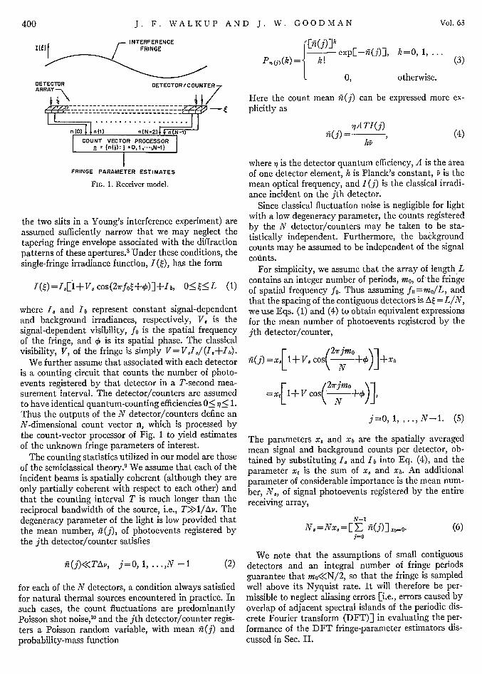
As shown in Fig. 1, the receiver is modeled as a one-dimensional array of N contiguous, identical photo-emissive detectors. (Extension of the major results totwo-dimensional geometries is straightforward, and ismentioned briefly in Sec. VI.) Each detector is assumedto have a transverse dimension that is much smallerthan the fringe period, thus permitting us to neglect thesmoothing effects caused by finite detector size.

We assume two-beam interference with quasimono-chromatic, plane-polarized beams of thermal light. Thetwo apertures from which the light beams arise (e.g.,

399Copyright e 1973 by the Optical Society of America.

J. F. WALKUP AND J. W. GOODMAN

INTERFERENCE

DETECTOR DETECTOR/COUNTERARRAY-

A..... ......n(O) n(1) n(N-2) n N-i

COUNT VECTOR PROCESSORn {n(j):j O,1, ,N-I}

FRINGE PARAMETER ESTIMATES

FIG. 1. Receiver model.

the two slits in a Young's interference experiment) areassumed sufficiently narrow that we may neglect thetapering fringe envelope associated with the diffractionpatterns of these apertures.8 Under these conditions, thesingle-fringe irradiance function, I(Q), has the form

I(Q)=IE1+V, cos(2rfot+0)]+Ib, 0<•<L (1)

where I, and Ib represent constant signal-dependentand background irradiances, respectively, V, is thesignal-dependent visibility, fo is the spatial frequencyof the fringe, and ' is its spatial phase. The classicalvisibility, V, of the fringe is simply V= VsIs/(Is+Ib).

We further assume that associated with each detectoris a counting circuit that counts the number of photo-events registered by that detector in a T-second mea-surement interval. The detector/counters are assumedto have identical quantum-counting efficiencies 0• _< 1.Thus the outputs of the N detector/counters define anN-dimensional count vector n, which is processed bythe count-vector processor of Fig. 1 to yield estimatesof the unknown fringe parameters of interest.

The counting statistics utilized in our model are thoseof the semiclassical theory. 9 We assume that each of theincident beams is spatially coherent (although they areonly partially coherent with respect to each other) andthat the counting interval T is much longer than thereciprocal bandwidth of the source, i.e., T>>1/Av. Thedegeneracy parameter of the light is low provided thatthe mean number, h(j), of photoevents registered bythe jth detector/counter satisfies

i (j)<<TAv, j = 0, 1, .. .,N -1 (2)

for each of the N detectors, a condition always satisfiedfor natural thermal sources encountered in practice. Insuch cases, the count fluctuations are predominantlyPoisson shot noise,"0 and the jth detector/counter regis-ters a Poisson random variable, with mean ii(j) andprobability-mass function

) [ exp[-fi(j)], k=O, 1, ...

L 0, otherwise.

Here the count mean Ti(j) can be expressed more ex-plicitly as

27A TI(j)fl(j) , (4)

where iq is the detector quantum efficiency, A is the areaof one detector element, h is Planck's constant, P is themean optical frequency, and I (j) is the classical irradi-ance incident on the jth detector.

Since classical fluctuation noise is negligible for lightwith a low degeneracy parameter, the counts registeredby the N detector/counters may be taken to be sta-tistically independent. Furthermore, the backgroundcounts may be assumed to be independent of the signalcounts.

For simplicity, we assume that the array of length Lcontains an integer number of periods, mi, of the fringeof spatial frequency fo. Thus assuming fo=mo/L, andthat the spacing of the contiguous detectors is At =L/N,we use Eqs. (1) and (4) to obtain equivalent expressionsfor the mean number of photoevents registered by thejth detector/counter,

*i(j) =xs[1+V. cos( 2 rjmo +0 ]+XbN l

L=x ii Vcos( +0),

j=0, 1, .., N-1. (5)

The parameters x, and Xb are the spatially averagedmean signal and background counts per detector, ob-tained by substituting I, and lb into Eq. (4), and theparameter xt is the sum of xs and Xb. An additionalparameter of considerable importance is the mean num-ber, N,, of signal photoevents registered by the entirereceiving array,

N-1N.=Nx.=[ rn(j)]b=O- (6)

j=0

We note that the assumptions of small contiguousdetectors and an integral number of fringe periodsguarantee that mo<<N/2, so that the fringe is sampledwell above its Nyquist rate. It will therefore be per-missible to neglect aliasing errors [i.e., errors caused byoverlap of adjacent spectral islands of the periodic dis-crete Fourier transform (DFT)] in evaluating the per-formance of the DFT fringe-parameter estimators dis-cussed in Sec. II.

Vol. 63400

FRINGE-PARAMETER ESTIMATION AT LOW LEVELS

II. THE DISCRETE FOURIER TRANSFORM AS AFRINGE-PARAMETER ESTIMATOR

One simple fringe-parameter estimator is the DFT.The amplitude and phase of the DFT at index mo yieldestimates of the peak amplitude and the phase of anincident fringe that contains mo periods across the array.

The N complex DFT components for the sequence(n(j):j=0, 1,. . ., NI-1) are defined by"'

1 N-iX(m) =- n(j) exp[-i22rjm/NJ,

N o

m=0, 1, ... , N-1. (7)

Alternatively, X(m) can be expressed in terms of itsreal and imaginary parts, respectively, defined by

1 N-I 2rjmR(m) =- n(j) cos - , (8)

N j=o N)

1 N-1 2i7rjmIm=--E n(j) sin ( . (9)

N j=o N

In all cases, the parameter m is a frequency index thatruns from 0 to N-1, with the actual spatial frequencycorresponding to the mth component being fm=m/L.The complex DFT component X(m) may also be ex-pressed in polar form in terms of a modulus r(m) and aphase 0(m). Thus,

X(MO) p (MO)

I

I I(M.,)

0 IMI.., ._ - ,.

DR(MJ)

FIG. 2. Phasor diagram for the moth DFT component.

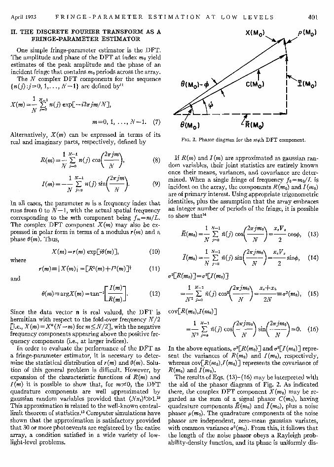
If R (m) and I(m) are approximated as gaussian ran-dom variables, their joint statistics are entirely knownonce their means, variances, and covariance are deter-mined. When a single fringe of frequency fo=mo/L isincident on the array, the components R(mo) and I(mo)are of primary interest. Using appropriate trigonometricidentities, plus the assumption that the array embracesan integer number of periods of the fringe, it is possibleto show that 14

1 N-I /2wrjmo\ XSVsR(mo)=- E fi(j) cos ) =5 cos4,

N j=o N1 2

X(m) =r(m) exp[i0(m)],where

r(m)s | X(m) I = [R2 (m) +I2 (m)]6

F 1(m)a0(m)margX(m) =tanii- R I.

(10)

(11)

(12)

Since the data vector n is real valued, the DFT ishermitian with respect to the fold-over frequency N/2[i.e., X(m) =X*(N-m) for m<N/2], with the negativefrequency components appearing above the positive fre-quency components (i.e., at larger indices).

In order to evaluate the performance of the DFT asa fringe-parameter estimator, it is necessary to deter-mine the statistical distribution of r(m) and 0(m). Solu-tion of this general problem is difficult. However, byexpansion of the characteristic functions of R(m) and1(m) it is possible to show that, for m$d0, the DFTquadrature components are well approximated bygaussian random variables provided that (Nxt)1>>1.'2

This approximation is related to the well-known central-limit theorem of statistics."3 Computer simulations haveshown that the approximation is satisfactory providedthat 30 or more photoevents are registered by the entirearray, a condition satisfied in a wide variety of low-light-level problems.

1 N-1 2irjmo\1(mo) = -EF i( j) sin

N j=0o

472[R(mo) ] =o2[I(mo)]

xs Vs= sino,

2

1 N-1 2 rjmO Xs+Xb

=-- E n(j) Cos2 = a-(mO)N2 j=O N 2N

cov[R(mo),I(mo)]

1 N-1 I2-wJmo\ 27rjmin=- fn(j) cos( sin =0.

N2 j--o \N / N

(13)

(14)

(15)

(16)

In the above equations, a-2[R(mo)] and uE[I(mo)] repre-sent the variances of R(mo) and I(mo), respectively,whereas cov[R(mo),I(mo)] represents the covariance ofR(mo) and I(mo).

The results of Eqs. (13)-(16) may be interpreted withthe aid of the phasor diagram of Fig. 2. As indicatedthere, the complex DFT component X(mo) may be re-garded as the sum of a signal phasor C(mo), havingquadrature components (mo) and 1(mo), plus a noisephasor p(mo). The quadrature components of the noisephasor are independent, zero-mean gaussian variates,with common variance a2 (mo). From this, it follows thatthe length of the noise phasor obeys a Rayleigh prob-ability-density function, and its phase is uniformly dis-

April 1973 401

v


lCI'I-1III

I

(18)

aWa:

at

zW

0a:crwowl

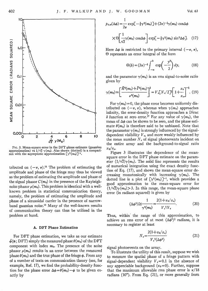
0.01 - For -y(mo) =0, the phase error becomes uniformly dis-tributed on (-7r, 7r), whereas when -y(m0) approachesinfinity, the error-density function approaches a Diraca function at zero error.'7 For any value of y(mo), themean of AO can be shown to be zero, and the phase esti-mate 0(mo) is therefore said to be unbiased. Note that

0.001 , I , I * X the parameter Py (mo) is strongly influenced by the signal-0 2 4 6 8 1 0 dependent visibility V8, and more weakly influenced by

I y(M0 ) the mean number N, of signal photoevents incident on24 the entire array and the background-to-signal ratio

FIG. 3. Mean-square error in the DFT phase estimate (gaussian xb/x,.proximation) vs 1/V7 -y(mno). Also shown (dotted) is a compari- Fann with the asymptotic approximation [y2 (,,mo)]-1. Figure 3 illustrates the dependence of the nean-

square error in the DFT phase estimate on the param-eter (1/<V)-y(mo). The solid line represents the results

ibuted on (-wr, 7r).1" The problem of estimating the of numerical integration using the exact density func-nplitude and phase of the fringe may thus be viewed tion of Eq. (17), and shows the mean-square error de-the problem of estimating the amplitude and phase of creasing monotonically with increasing y (no). The

.e signal phasor C(m) in the presence of the Rayleigh- dotted line is a plot of [,y2(mo)]I-, which provides aie s Ti te . . good approximation to the mean-square error for

oise phasor p (mo). This problem is identical with a well- (1/V)-y (mo) >3. In this range, the mean-square phaseiown problem in statistical communication theory, error (in radians squared) is given by

namely, the problem ot estimating the amplitude andphase of a sinusoidal carrier in the presence of narrow-band gaussian noise.1 6 Many of the well-known resultsof communication theory can thus be utilized in theproblem at hand.

A. DFT Phase Estimation

For DFT phase estimation, we take as our estimate(n; DFT) simply the measured phase 0(mo) of the DFT

component with index mo. The presence of the noisephasor p(mo) results in an error between the measuredphase 0(mo) and the true phase of the fringe p. From anyof a number of texts on communication theory (see, forexample, Ref. 17), we find the probability-density func-tion for the phase error Aq=0(mo)-k to be given ex-actly by

1 2(1+xb/x,)( 2()2) i V =

ly2(MO) Vs2 N.(20)

Thus, within the range of this approximation, toachieve an rms error of at most (AI2)- radians, it isnecessary to register at least

2(1 +Xb/X,)N,, =

V32(AO 2)(21)

signal photoevents on the array.To illustrate the utility of this result, suppose we wish

to measure the spatial phase of a fringe pattern withsignal-dependent visibility V,= 0.1 in the absence ofany appreciable background (Xb=0). Further, supposethat the maximum allowable rms phase error is nr/18radians (10°). From Eq. (21), or more generally from

1p~a(Ak) =-exp[-21y2(m.)]+ (2.)-)y(mo) cosAk

2r

X [- (mO) cosLX4] expE-[ y2(mo) sin2zXp]. (17)

Here AO is restricted to the primary interval (-7r, 7r),e- represents an error integral of the form

1.0

0.1 and the parameter -y (mo) is an rms signal-to-noise ratiogiven by

rR2(jmO)+j2(mo) i Xab -1

'y(m o) )-1L= V.ENV 122]{I+- . (19)-L cr2(mo) IiX

03

zUw

apSO]

trarass

thnc

0(b) = (27)-4f exp(--- ) dy,

402 Vool. 63


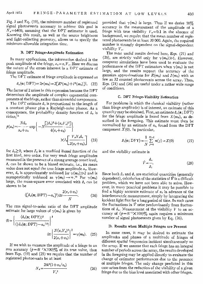
Fig. 3 and Eq. (19), the minimum number of registeredsignal photoevents necessary to achieve this goal isN8 =6400, assuming that the DFT estimator is used.Knowing this result, as well as the source brightnessand light-collecting geometry, allows us to specify theminimum-allowable integration time.

B. DFT Fringe-Amplitude Estimation

In many applications, the information desired is thepeak amplitude of the fringe, a,=x V8 . Here we discussthe nature of the errors inherent in a DFT estimate offringe amplitude.

The DFT estimate of fringe amplitude is expressed as

d,(n; DFT)-2r(mo)=2[R2 (mo)+I2(mo)]1. (22)

The factor of 2 arises in this expression because the DFTdetermines the amplitude of complex exponential com-ponents of the fringe, rather than sinusoidal components.

The DFT estimate d, is proportional to the length ofa constant phasor plus a Rayleigh-noise phasor. As aconsequence, the probability density function of da isrician,'8

Nas(as)=: exp

XS+Xb[(a 2+(x 8 V )2]

4(X8+Xb)

F ViSNad 1XIo

-2(X++Xb)i(23)

for d8 ŽO, where 1o is a modified Bessel function of thefirst kind, zero order. For very weak fringe amplitudesmeasured in the presence of a strong average count level,as can be shown to be a biased estimate, i.e., its meanvalue does not equal the true fringe amplitude a,. How-ever, a, is approximately unbiased for -y(mo)>2 and isasymptotically unbiased as y (mo) -* *'. For -y (mo)large, the mean-square error associated with da can beshown to be

([d8(n; DFT) -aj] 2)- V * (24)N

The rms signal-to-noise ratio of the DFT amplitudeestimate for large values of -y(mo) is given by

(48(n; DFT))2 11

l(1d4(n; DFT) -aas 2)f

N(XsVs)2] i

2(X.,+Xb) =y(mo). (25)

If we wish to measure the amplitude of a fringe to anrms accuracy (p=G1-'X100)% of its true value, thenfrom Eqs. (19) and (25) we require that the number ofregistered photoevents be at least

N8 = 26R2(1+Xb/xS)

V82 (26)

provided that y (mo) is large. Thus if we desire 10%accuracy in the measurement of the amplitude of afringe with true visibility V, = 0.1 in the absence ofbackground, we require that the mean number of regis-tered photoevents be at least 20 000. Again, the requirednumber is strongly dependent on the signal-dependentvisibility Vs.

The most useful results derived here, Eqs. (21) and(26), are strictly valid only for 'y(mo)>l. However,computer simulations have been used to evaluate theperformance of the DFT estimators when -y(mo) is notlarge, and the results support the accuracy of thegaussian approximations for Rn(mo) and I(mo) with asfew as 32 counted photoevents across the array. Thus,Eqs. (21) and (26) are useful under a rather wide rangeof conditions.

C. DFT Fringe-Visibility Estimation

For problems in which the classical visibility (ratherthan fringe amplitude) is of interest, an estimate of thisquantity may be obtained. First, an estimate da (n; DFT)for the fringe amplitude is found from X(mo), as de-scribed in the foregoing. This estimate must then benormalized by an estimate of xt, found from the DFTcomponent X(0). In particular,

1 N-1&t(n;DFT)=- E n(j)==X(0)

N j=o

and the visibility estimate is

a,

(27)

(28)

Since both &t and as are statistical quantities (generallydependent), calculation of the statistics of f2 is a difficultproblem, which we have not been able to solve. How-ever, in many practical problems it may be possible tofind a highly accurate estimate of xt in advance of theinterferometric measurement, simply by integrating theincident light flux for a long period of time. In such casesthe fluctuations in 1T arise predominantly from fluctua-tions of as. Measurement of the visibility V to an ac-curacy of (p=R-'X100)% again requires a minimumnumber of signal photoevents given by Eq. (26).

D. Results when Multiple Fringes are Present

In some cases, it may be desired to estimate theamplitudes and phases of a multitude of fringes ofdifferent spatial frequencies incident simultaneously onthe array. If we assume that each fringe has an integralnumber of periods across the array, the results developedin the foregoing may be applied directly to evaluate thechange of estimator performances due to the presenceof multiple fringes. The only change predicted in thiscase arises from the reduction of the visibility of a givenfringe due to the bias level associated with other fringes.

April 1973 403


In particular, the parameter y is now given by(NtV2/2)1, where Nt is the total number of photoeventsand V is the classical visibility of the fringe in question.

We have throughout assumed that the fringes havean integral number of periods across the array. If this isnot the case, the DFT estimates suffer from a phe-nomenon known as leakage."' 20 The major effects ofleakage are to lower the signal-to-noise ratio y(rno) forthe DIET estimators and to introduce biases into theestimates of visibility and phase.2 ' Various techniquesare available for compensating for the degrading effectsof leakage,20 but this subject will not be treated here.

Ill. JOINT-MAXIMUM-LIKELIHOODESTIMATION

The DFT estimators discussed in Sec. II arose purelyfrom intuitive reasoning, rather than from any par-ticular optimality criterion. Given the observed countvector n of independent Poisson random variables, thejoint-maximum-likelihood (JMIL) estimators operate onthat data vector to solve for the fringe-parameter valuesthat jointly maximize the probability of observing thatparticular data vector.2 2'23

To derive the JML estimators, we let a denote theset of fringe parameters to be estimated, and make useof the conditional independence of the N elements ofthe vector n to write the likelihood function

N-1 N-i EiV{)1niP(n II) II P{Jt a) = H exp[-fij(a). (29)

j=0 Ho e n!

Rather than maximize P(nlIa), we may alternativelymaximize the log likelihood function

A(n I a)-lnP(nI a)

X-I= E:-lnnj!-%fi{(e)+nj lnhy(a)]. (30)

Since the first term of Eq. (30) is independent of theparameter set a, we may alternatively maximize thereduced log likelihood function

N-1Ao(n I a) = Z E [-FIXa)+nj lnii(a)J, (31)

j=O

where, based on Eq. (5)$ we write tij(a) in the form

Fjy(a) =Xf i+Vcost27rmo ,

j=0, 1, ... , N-1 (32)

with Xt=X 3 +Xb, V=x3 V3 /(x 8 +xb), and xtV =x 3 V7=a 8.

To permit comparisons with the DIFT estimators, wechoose to maximize Eq. (31) with respect to the param-eter vector a = (s,xsa2). This maximization requires the

solution of three homogeneous equations24

OAo(n a)=0, i=1, 2, 3, (33)

where ai=4, a 2 =Xj, and aa=aa. For arbitrary visibili-ties, the resulting equations are coupled and closed formsolutions do not appear possible. However, if we imposea low-visibility constraint, 0<V<<1, we may use thesmall-argument logarithmic approximation ln(l+x)Žx-4x 2 to uncouple the simultaneous equations. Theresulting uncoupled equations can then be solvedsequentially, yielding

dn; JML) = tanr-{ -7 sin'ko NT

> :nj cos ),

1 N-I±,(n; JML)=- Z nj,

]Nj 1=0

(34)

(35)

a3 (n; JML)=&x(n; JML)

Nx I 27rmo J

N-1 227rjmoFE, co&CO +t(n; JML)IL

y=_o N I J(36)

The JML estimate of the classical visibility is2B

a3 N-i 1 27rjmol(; JML)= =E nj cos- -4(n; JML)J/

iY-I - 7 fo A N

>E n1 cos'[t+&n; JML)]. (37)

That these solutions actually correspond to maxima ofthe reduced log likelihood function has been verified byshowing that the second partial derivatives of AO withrespect to the individual parameters are negative at theJML estimates, except in degenerate cases.

It is useful to make some comparisons between theJML estimators of Eqs. (34)-(37) and the DFT esti-mators discussed in Sec. II. By comparing Eqs. (12) and(34), we see that the DFT phase estimate is identicalwith the low-visibility JiML phase estimate. In addi-tion, by substituting Eqs. (34) and (35) into (36), andcomparing the result with Eq. (22), we find that

4/tn; DIET)da(n; JML) = [,/(n; JML)]1+[C(n,0)1&,(n; JML)]'

(38)

404 vol. 63


where

1 N-1 47rjmoQn, E nj cos +24(n; JML) .

N j=o N

We can readily show that

(CQn,+)) =0,

Xt

[, C(n,0)]-,2N

(&t) Xt,

a hybrid parameter, and its Cram6r-Rao bound can bedetermined by use of the relationship23

(39)3 a9V OV

E[~)V]2> E _Jjji d-l d9ai (9ai

(43)

Proceeding as indicated above, and using a low-visi-bility constraint 0<V<<1 to simplify the mathematics,we obtain for the CRB's

(40)

N

We can then show that the value of the bracketed termin Eq. (38) will be much less than unity provided thatthe total number, Nxt, of recorded photoevents is muchlarger than unity. Thus, the DFT and JML estimatorsof fringe amplitude are essentially the same, providedthat Nxt>>1. Finally, we note that the JML estimate ofxt is identical with the zero-frequency component ofthe DFT.

To summarize this section, we have shown that a closerelationship exists between the DFT fringe-parameterestimators and the low-visibility JML estimators. Theseresults lend strong support to the use of DFT estimatorsin applications such as interferometric image synthesis,2 6

in which the fringes associated with high spatial fre-quencies will generally have low visibility.

IV. CRAMfR-RAO PERFORMANCE BOUNDS

The application of basic results from estimation the-ory permits us to derive lower bounds on the mean-square errors achievable by any unbiased multiparam-eter estimators of the fringe parameters. Such boundsare known as the Cram6r-Rao performance bounds.22'23

If we assume a k-dimensional parameter vector a, themultiparameter Cramer-Rao bound (CRB) for the ithelement of a may be written

E[ai(n)-ax]2>Jii=CRB(ai), i=1, 2,..., k (41)

where E[ ] indicates an expectation operator. Here jiis the i-ith element of the kXk inverse of Fisher's in-formation matrix (elements Jjj), which is defined by23

Ji= -E a , i, j=1, 2, ... ,k. (42)

The quantity P(n I a) is again given by Eq. (29). Anyestimate that achieves the bound is called an efficientestimate.

Equations (41) and (42) have been used to evaluatethe Cramer-Rao error bounds for the parameter vectora= (,a,,xt). The parameter V=a,/x, can be viewed as

2CRB(O) =X

NXtV2

2xtCRB(a,)-,

* N

XtCRB(xt) =-,

N

2CRB(V) =

Nxt

Y(mO)»> (44)

(45)

(46)

(47)

Some comment is required regarding the bound for 4.The stated bound is valid only when y(mo)>l, becausethe derivation does not take into account the fact thatphase estimates are restricted to the interval (-7r,7r).In practice, the mean-squared error of the phase esti-mate cannot exceed (2 7r)2/12, the variance of a uni-formly distributed phase on (-7r, 7r). However, forlarge -y (no), the differences between modulo-27r andnonmodulo-27r definitions of phase become insignificant,and the error bound Eq. (44) is applicable.

The results represented by Eqs. (44)-(47) are funda-mental bounds on the performances of all unbiased esti-mators. Of particular interest are the relationships be-tween these bounds and the actual performances of theDFT parameter estimators. The zero-frequency com-ponent of the DFT is seen to be an efficient estimatorof xt, since it is unbiased and achieves the CRB. TheDFT estimator of phase is likewise efficient, providedthat ty(mo) is large. The DFT estimator for a, is biasedfor low y(mo); the CRB does not apply under this con-dition. However, for y(mo)>1, the DFT estimator isasymptotically unbiased, and comparison of Eqs. (45)and (24) show that it, too, is efficient. Because we wereunable to evaluate the variance of the DFT estimator ofV, we can make no comparison with the CRB in thiscase. With respect to xt, 0, and a, however, we can con-clude that for y (mo)>1, no unbiased estimator can per-form better than the DFT.

V. SPATIAL vs TEMPORAL SAMPLINGOF THE FRINGE

In this section we apply the basic analytical tech-niques of Sec. II to compare the theoretical performanceof the N-detector spatial-sampling method discussed

April 1973 405


output, the combination of time gating and countingpermits determination of the number of photoeventsregistered during consecutive intervals of At seconds(A~t<l/Av 3 ). We assume that A\t is large compared withthe reciprocal bandwidth of the incident light, and thatthere are N' consecutive counting intervals in the totalmeasurement time T' (i.e., T'=N'At). We further as-sume that the interval T' contains an integral numberino' of periods of the temporal fringe (mo'= T'Av,).

Based on the temporal-fringe-irradiance function andthe assumed low degeneracy of the light, the number ofphotoevents registered in each of the N' counting in-tervals may be modeled as statistically independentPoisson variates. The mean number of counts for thejth detection interval is

ii(j)=xt'l+-cost +o]

j=0, 1, ..., N'-1 (51)where for an effective detector area a,

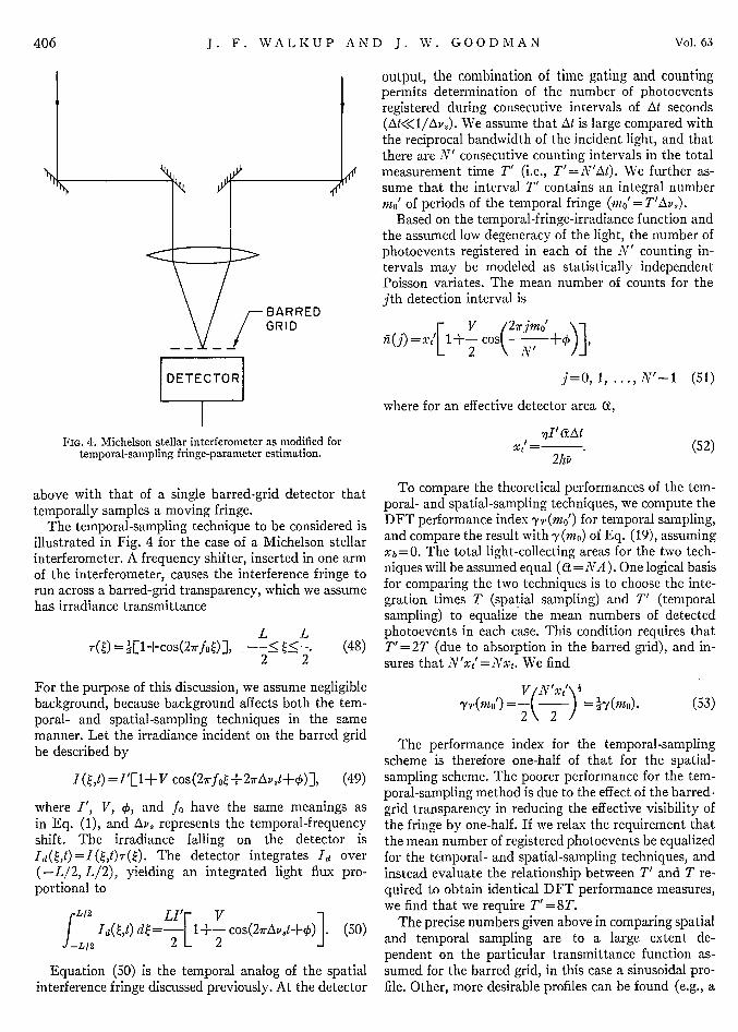
FIG. 4. Michelson stellar interferometer as modified fortemporal-sampling fringe-parameter estimation.

above with that of a single barred-grid detector thattemporally samples a moving fringe.

The temporal-sampling technique to be considered isillustrated in Fig. 4 for the case of a Michelson stellarinterferometer. A frequency shifter, inserted in one armof the interferometer, causes the interference fringe torun across a barred-grid transparency, which we assumehas irradiance transmittance

L LTQ) = l[l+cos(27rfot)], .- - (48)

2 2

For the purpose of this discussion, we assume negligiblebackground, because background affects both the tem-poral- and spatial-sampling techniques in the samemanner. Let the irradiance incident on the barred gridbe described by

I (,t) =1'[l+V cos(2xrfo+27rAzvst+0)], (49)

where I', V, X, and fo have the same meanings asin Eq. (1), and AP,, represents the temporal-frequencyshift. The irradiance falling on the detector isId(0,t)=I(Q,t)r(r). The detector integrates Id over(-L/2, L/2), yielding an integrated light flux pro-portional to

JL/2 LI'[ V|UV~~) d(=-1+- cos(2rAv,,t+0) . (50)

L/2 2 2

Equation (50) is the temporal analou of the spatialinterference fringe discussed previously. At the detector

qI'G La

2hp(52)

To compare the theoretical performances of the tem-poral- and spatial-sampling techniques, we compute theDFT performance index YT(MO') for temporal sampling,and compare the result with -y(mo) of Eq. (19), assumingXb=O. The total light-collecting areas for the two tech-niques will be assumed equal (a =NA). One logical basisfor comparing the two techniques is to choose the inte-gration times T (spatial sampling) and T' (temporalsampling) to equalize the mean numbers of detectedphotoevents in each case. This condition requires thatT'=2T (due to absorption in the barred grid), and in-sures that N'xt'=Nxt. We find

VT N'x) =.= I'YT(,mo') =-{ 2-Y(mo)-

2\ 2/(53)

The performance index for the temporal-samplingscheme is therefore one-half of that for the spatial-sampling scheme. The poorer performance for the tem-poral-sampling method is due to the effect of the barred-grid transparency in reducing the effective visibility ofthe fringe by one-half. If we relax the requirement thatthe mean number of registered photoevents be equalizedfor the temporal- and spatial-sampling techniques, andinstead evaluate the relationship between T' and T re-quired to obtain identical DFT performance measures,we find that we require T'=8T.

The precise numbers given above in comparing spatialand temporal sampling are to a large extent de-pendent on the particular transmittance function as-sumed for the barred grid, in this case a sinusoidal pro-file. Other, more desirable profiles can be found (e.g., a

BARREDGRID

406 Vol. 63


square wave, which reduces the visibility by a factor of2 /7r rather than 2); the use of partially reflecting struc-tures with two detectors can improve performancefurther. However, in all cases, the performance of thespatial-sampling scheme provides an upper bound to theperformance of more economical and practical temporal-sampling schemes, if we assume that equal amounts ofenergy are available for the measurements.

VI. CONCLUDING REMARKS

Use of a spatial-sampling receiver model has enabledus to define the fundamental limitations, at low lightlevels, in estimating the amplitude and phase of aninterference fringe. The range of applicability of theseresults is broad. Though the previous calculations as-sumed a one-dimensional receiver geometry, the resultsare easily extended to the more practical two-dimen-sional format. The no-leakage requirement restricts usto a finite number of possible fringe angles with respectto the perpendicular coordinate axes, but if the numberof detectors is large, the number of allowable angles islarge. Given these minor additional considerations,there are no conceptual difficulties in applying our re-sults to two-dimensional detector arrays.

REFERENCES

*Work sponsored by the Office of Naval Research and by theStanford Joint Services Electronics Program.

'W. I. Beavers, Astron. J. 68, 273 (1963).2J. L. Elliot, M. S. thesis, Department of Physics, Massachusetts

Institute of Technology (1965).

3W. I. Beavers and W. D. Swift, Appl. Opt. 7, 1975 (1968).4 E. S. Kulagin, Opt. Spektrosk. 23, 839 (1967) [Opt. Spectrosc.

23, 459 (1967)].5J. S. Wilczynski, J. Opt. Soc. Am. 57, 579 (1967).6W. T. Rhodes, Ph.D. thesis, Department of Electrical

Engineering, Stanford University (1971) (UniversityMicrofilms, Ann Arbor, Mich., order No. 72-16 780).

7M. Born and E. Wolf, Principles of Optics, 2nd ed. (Pergamon,New York, 1964), p. 501.

8Reference 7, p. 515.9L. Mandel, in Progress in Optics, II, edited by E. Wolf

(North-Holland, Amsterdam, 1963), pp. 181-248.10 L. Mandel, Proc. Phys. Soc. Lond. 74, 233 (1959)."G. D. Bergland, IEEE Spectrum 6 (7), 41 (1969).12J. Walkup, Ph.D. thesis, Department of Electrical

Engineering, Stanford University (1971) (UniversityMicrofilms, Ann Arbor, Mich., order No. 72-11 685).

13P. Beckmann, Probability in Communication Engineering(Harcourt, Brace, and World, New York, 1967), p. 106.

'4 Reference 12, p. 157.15Reference 13, p. 118.16J B. Thomas, Introduction to Statistical Communication

Theory (Wiley, New York, 1969), p. 160.17Reference 16, p. 167.'8Reference 16, p. 161.19Reference 12, p. 39.20 D. C. Rife and G. A. Vincent, Bell Syst. Tech. J. 49, 197

(1970).2 'Reference 12, p. 44.22R. Deutsch, Estimation Theory (Prentice-Hall, Englewood

Cliffs, N. J., 1965).23H. L. Van Trees, Detection, Estimation, and Modulation

Theory, Part I (Wiley, New York, 1968).2 4 Reference 12, p. 49.25

1t is possible to maximize A0 with respect to the expandedparameter set (4<,x,, V,a,). However, of the four equationsgenerated, only three are linearly independent. The estimateV obtained is identical with Eq. (37).26J. W. Goodman, J. Opt. Soc. Am. 60, 506 (1970).

COPYRIGHT AND PERMISSION

This Journal is fully copyrighted, for the protection of the authors andtheir sponsors. Permission is hereby granted to any other authors to quotefrom this journal, provided that they make acknowledgment, includingthe authors' names, the Journal name, volume, page, and year. Reproduc-tion of figures and tables is likewise permitted in other articles and books,provided that the same information is printed with them. The best andmost economical way for the author and his sponsor to obtain copies is toorder the full number of reprints needed, at the time the article is printed,before the type is destroyed. However, the author, his organization, orhis government sponsor are hereby granted permission to reproduce partor all of his material. Other reproduction of this Journal in whole or inpart, or copying in commercially published books, periodicals, or leafletsrequires permission of the editor.

April 1973 407

limitations of fringe-parameter estimation at low light levels

Documents