LIFT, DRAG AND MOMENT OF A NACA 0015 AIRFOIL

by Steven D. Miller

DEPARTMENT OF AEROSPACE ENGINEERINGTHE OHIO STATE UNIVERSITY

i28 MAY 2008

ABSTRACTA NACA 0015 symmetrical airfoil with a 15% thickness to chord ratio was analyzed to determine the lift, drag and moment coefficients. A 2D airfoil was placed in a low speed wind tunnel with pressure taps along its surface and a pitot probe downstream to measure the flow characteristics. The wind tunnel was operated at a nominal 17 m/s during the coefficient measurements, a Reynold's number of about 232,940. The airfoil, with an 8 in chord, was analyzed at 0, 5, 10 and 15 degree angles of attack. The phenomenon known as hysteresis with regards to stall conditions was also observed by varying the angle of attack and wind tunnel velocity.

ii

TABLE OF CONTENTS PageList of Figures ivList of Tables ivNomenclature vChapter I. Introduction 1 II. Apparatus and Instrumentation 2 III.Experimental Procedure 4 IV. Analysis 5 V. Results and Discussion 7 VI. Conclusions 13Appendix 14References 18

iii

LIST OF FIGURES

LIST OF TABLES

iv

Figure Page1 NACA 0015 Airfoil Cross-section with Pressure Taps 22 Pressure Distribution at 0 Deg Angle of Attack 83 Pressure Distribution at 5 Deg Angle of Attack 94 Pressure Distribution at 10 Deg Angle of Attack 95 Pressure Distribution at 15 Deg Angle of Attack 106 Velocity Profile of the Downstream Wake 11

Tables Page1 Lift, Drag and Moment Coefficients 12

NOMENCLATURE

v

c Chordf Functionu VelocityCoefficient of DragCoefficient of FrictionCoefficient of LiftMoment CoefficientCoefficient of PressureD DragI IntegralReynold's Numberu Free Stream VelocityAngle of AttackDensity

CDCfCLCMCp

Re

αρ

INTRODUCTIONThis experiment analyzes the NACA 0015 airfoil in a low speed wind tunnel at varying angles of attack. The NACA 0015 is a symmetrical airfoil with a 15% thickness to chord ratio. Symmetric airfoils are used in many applications including aircraft vertical stabilizers, submarine fins, rotary and some fixed wings. A 2D wing section is analyzed at low speeds for lift, drag and moment characteristics. A second goal of the experiment was to observe the hysteresis effect of the stall speed and angle of attack. This is important to understanding the stall characteristics of this airfoil.

1

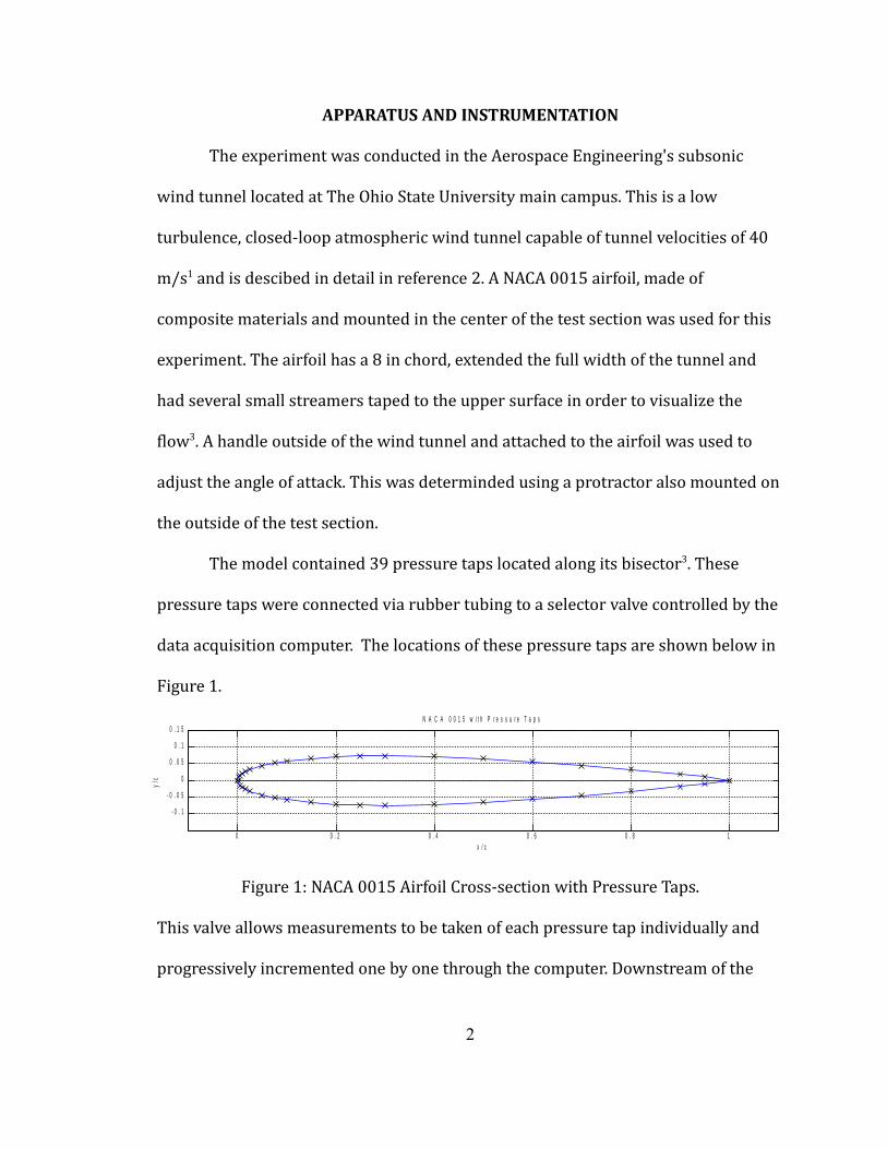
APPARATUS AND INSTRUMENTATIONThe experiment was conducted in the Aerospace Engineering's subsonic wind tunnel located at The Ohio State University main campus. This is a low turbulence, closed-loop atmospheric wind tunnel capable of tunnel velocities of 40 m/s1 and is descibed in detail in reference 2. A NACA 0015 airfoil, made of composite materials and mounted in the center of the test section was used for this experiment. The airfoil has a 8 in chord, extended the full width of the tunnel and had several small streamers taped to the upper surface in order to visualize the flow3. A handle outside of the wind tunnel and attached to the airfoil was used to adjust the angle of attack. This was determinded using a protractor also mounted on the outside of the test section. The model contained 39 pressure taps located along its bisector3. These pressure taps were connected via rubber tubing to a selector valve controlled by the data acquisition computer. The locations of these pressure taps are shown below in Figure 1.

Figure 1: NACA 0015 Airfoil Cross-section with Pressure Taps.This valve allows measurements to be taken of each pressure tap individually and progressively incremented one by one through the computer. Downstream of the 2

0 0 . 2 0 . 4 0 . 6 0 . 8 1

- 0 . 1

- 0 . 0 5

0

0 . 0 5

0 . 1

0 . 1 5N A C A 0 0 1 5 w i t h P r e s s u r e T a p s

x / c

y/c

airfoil, a total pressure pitot probe is mounted on the computer controlled traverse. This is set-up to take pressure measurements in the flow while traversing the wake of the airfoil vertically. In order to measure the dynamic pressure from this, the static pressure is measured from a pitot-static probe located 3 inches from the top and 6 inches downstream from the beginning of the test section.

3

EXPERIMENTAL PROCEDUREThe airfoil was set at a 0 degree angle of attack and the wind tunnel operated at approximately 15 m/s3. The angle of attack was varied while taking note of the behavior of the small streamers on the suction side of the airfoil. The points of separation and reattachment were noted. The angle of attack was then set at approximately 15 degrees and the wind tunnel velocity varied again taking note of the streamers as the flow separates and reattaches at various speeds.The wind tunnel velocity was then set at a nominal 17 m/s for the remainder of the experiment3. The pressure distribution about the aifoil's pressure taps was recorded at set angles of attack of 0, 5, 10 and 15 degrees. The airfoil was again placed at a 0 degree angle of attack and the downstream wake measured using the pitot probe and traverse.

4

ANALYSISThe trapezoidal rule is used several times throughout the analysis in order to numerically carry out required integration of the measured data. The following is the trapezoidal rule (method) also known as the trapezium rule4.I f ≈ [ f a f b ]

2b−a

This is a simple geometric approximation to the area under the curve f by assuming the change between any two points a and b is linear.The following four equations3 were used in order to determine the measured coefficients of lift and drag from the pressure tap data.

All integration required in these equations was accomplished using the trapezoidal rule described above. The moment coefficient was calculated about the quarter chord position taking the counterclockwise direction as positive. This was done with the following equation for the moment coefficient.

5

The NACA 0015 airfoil is relatively thin and symmetric. Because of this, thin airfoil theory was applied in order to determine the theoretical values of the lift, drag and moment coefficients. The following equation relates the coefficient of lift to the angle of attack for thin symmetrical airfoils5.C L=2 By this theory, the coefficient of the moment about the aerodynamic center of a thin symmetrical airfoil is zero and that the aerodynamic center is located at the quarter chord or x/c = 0.25. Therefore, the moment coefficient for any angle of attack at the quarter chord is zero by theory. The theoretical drag of the airfoil can be estimated by making a flat plate assumption and analyzing the laminar and turbulent cases separately5. The following equations apply to laminar and turbulent flow respectively.C f lam=

1.328Re

C f turb=0.074Re1 /5

These frictional coefficients are then added to the measured drag coefficient in order to determine the total drag coefficient.The drag can better be measured by traversing the wake downstream of the airfoil. This is done by analyzing the momentum loss of the fluid due to the viscous forces by applying the momentum theorem to a control volume around the airfoil3.

6

The following drag equation was used and normalized with the dynamic pressure.D= b∫

S 2

u2 U inf −u2 dS

S2 represents the surface area of the downstream face of the control volume where u2 is the velocity through it.

7

RESULTS AND DISCUSSIONWhile holding the tunnel velocity constant and varying the angle of attack characteristics of the flow can be seen in the attached streamers. As angle of attack is increased, the flow will eventually separate from the upper surface of the airfoil resulting in a 'stall'. It was noted that the angle of attack must be decreased below the separation angle of attack in order for the flow to reattach. This phenomenon is known as hysteresis. The same can be seen by setting the angle of attack and decreasing the tunnel velocity until separation occurs. The velocity must be increased again much higher than the velocity at which the flow separated in order to reattach.The following 4 figures are plots of the coefficient of pressure (Cp) versus the normalized x-location of the pressure tap. The upper surface taps are shown as blue +'s whereas the lower surface taps are shown as green *'s. Figure 2 shows the results with the airfoil set at a 0 degree angle of attack.

8

Figure 2: Pressure Distribution at 0 Deg Angle of Attack.For a 0 deg angle of attack the points on the upper and lower surfaces almost match exactly, a result of the symmetric airfoil. The upper pressure distribution of the 5 deg angle of attack plot, Figure 3, shows a slight jump in value at about the 0.35 x/c location.

9

0 0 . 1 0 . 2 0 . 3 0 . 4 0 . 5 0 . 6 0 . 7 0 . 8 0 . 9 1- 1

- 0 . 8

- 0 . 6

- 0 . 4

- 0 . 2

0

0 . 2

0 . 4

0 . 60 0 d e g A n g l e o f A t t a c k

x / c

-Cp

U p p e r S u r f a c e

L o w e r S u r f a c e

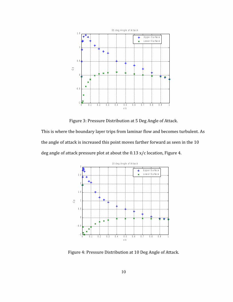
Figure 3: Pressure Distribution at 5 Deg Angle of Attack.This is where the boundary layer trips from laminar flow and becomes turbulent. As the angle of attack is increased this point moves farther forward as seen in the 10 deg angle of attack pressure plot at about the 0.13 x/c location, Figure 4.

Figure 4: Pressure Distribution at 10 Deg Angle of Attack.10

0 0 . 1 0 . 2 0 . 3 0 . 4 0 . 5 0 . 6 0 . 7 0 . 8 0 . 9 1- 1

- 0 . 5

0

0 . 5

1

1 . 50 5 d e g A n g l e o f A t t a c k

x / c

-Cp

U p p e r S u r f a c e

L o w e r S u r f a c e

0 0 . 1 0 . 2 0 . 3 0 . 4 0 . 5 0 . 6 0 . 7 0 . 8 0 . 9 1- 1

- 0 . 5

0

0 . 5

1

1 . 5

2

2 . 5

31 0 d e g A n g l e o f A t t a c k

x / c

-Cp

U p p e r S u r f a c e

L o w e r S u r f a c e

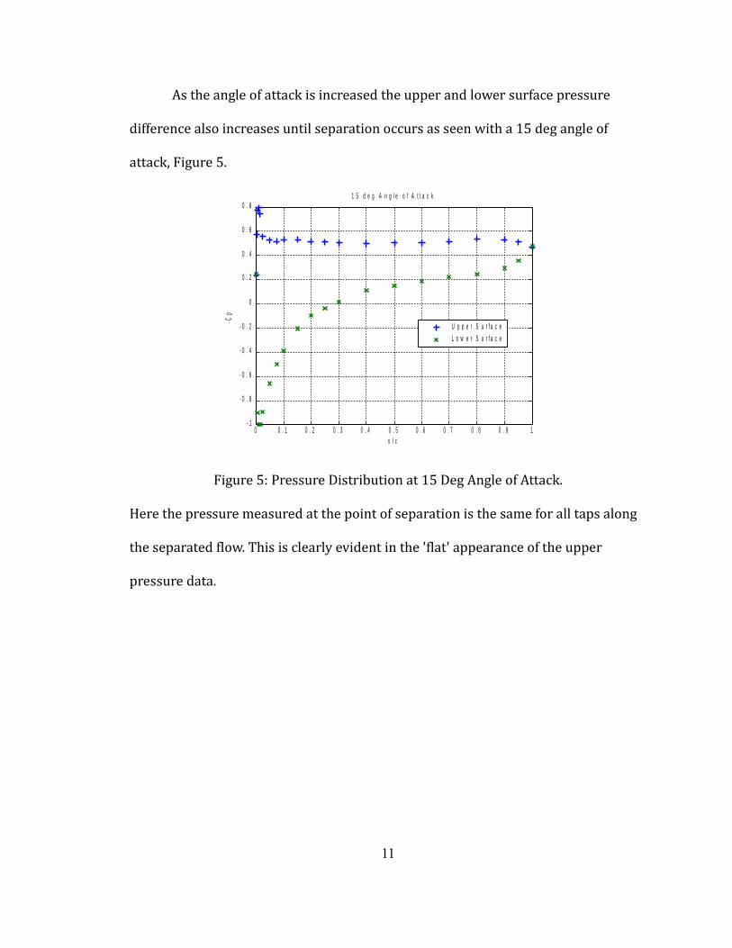
As the angle of attack is increased the upper and lower surface pressure difference also increases until separation occurs as seen with a 15 deg angle of attack, Figure 5.

Figure 5: Pressure Distribution at 15 Deg Angle of Attack.Here the pressure measured at the point of separation is the same for all taps along the separated flow. This is clearly evident in the 'flat' appearance of the upper pressure data.

11

0 0 . 1 0 . 2 0 . 3 0 . 4 0 . 5 0 . 6 0 . 7 0 . 8 0 . 9 1- 1

- 0 . 8

- 0 . 6

- 0 . 4

- 0 . 2

0

0 . 2

0 . 4

0 . 6

0 . 81 5 d e g A n g l e o f A t t a c k

x / c

-Cp

U p p e r S u r f a c e

L o w e r S u r f a c e

Figure 6 shows the plotted results of the wake traverse with the pitot probe.

Figure 6: Velocity Profile of the Downstream Wake.The vertical black line indicates the free stream velocity obtained by averaging the outermost data points that were well outside of the wake. The downstream profile very clearly shows the velocity and therefore momentum deficit in the flow do to the viscous (friction) losses to the airfoil.The following Table 1 contains all of the measured and theoretical values for the desired lift, drag and moment coefficients of the NACA 0015 airfoil.

12

1 4 1 5 1 6 1 7 1 80

1

2

3

4

5

6

7D o w n s t r e a m V e l o c i t y P r o f i l e

V e l o c i t y ( m / s )

Pos

ition

(cm

)

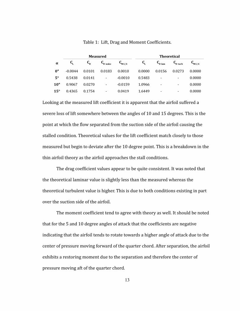
Table 1: Lift, Drag and Moment Coefficients.

Looking at the measured lift coefficient it is apparent that the airfoil suffered a severe loss of lift somewhere between the angles of 10 and 15 degrees. This is the point at which the flow separated from the suction side of the airfoil causing the stalled condition. Theoretical values for the lift coefficient match closely to those measured but begin to deviate after the 10 degree point. This is a breakdown in the thin airfoil theory as the airfoil approaches the stall conditions.The drag coefficient values appear to be quite consistent. It was noted that the theoretical laminar value is slightly less than the measured whereas the theoretical turbulent value is higher. This is due to both conditions existing in part over the suction side of the airfoil.The moment coefficient tend to agree with theory as well. It should be noted that for the 5 and 10 degree angles of attack that the coefficients are negative indicating that the airfoil tends to rotate towards a higher angle of attack due to the center of pressure moving forward of the quarter chord. After separation, the airfoil exhibits a restoring moment due to the separation and therefore the center of pressure moving aft of the quarter chord.13

Measured Theoretical

-0.0044 0.0101 0.0183 0.0010 0.0000 0.0156 0.0273 0.00005° 0.5438 0.0141 - -0.0010 0.5483 - - 0.00000.9067 0.0270 - -0.0159 1.0966 - - 0.0000

15° 0.4365 0.1754 - 0.0419 1.6449 - - 0.0000

α CL CD CD wake CM1/4 CL CD lam CD turb CM1/4

0°

10°

CONCLUSIONSThe NACA 0015 airfoil was analyzed for the lift, drag and moment coefficients as planned. The measured values determined from lab data agree correctly with the theoretical values for the lift, drag and quarter chord moment. A stabilizing or restoring moment was observed after the stall occurred. The coefficient tests were conducted at a nominal Reynolds number of 232,940.The hysteresis effect was clearly observed with respect to the separation conditions of free stream velocity and angle of attack. This was accomplished by visually observing the flow of the suction side of the airfoil with small attached streamers. Reynold's numbers varied between 94,000 and 235,000 for this observation.

14

APPENDIX

clc

clear allclose all% Steven D. Miller% Aerospace Engineering, The Ohio State University% Course: AAE 510.03% 2 May 2008 c=.2032; % chord length in mb=1; % unit spanx0=.25; % moment location % Read airfoil coordinate data from filefilename=('coord015.dat'); fid=fopen(filename,'r','l'); row=fread(fid,[1,1],'double'); col=fread(fid,[1,1],'double'); xc=zeros(row,col); xc=fread(fid,[row,col],'double'); fclose(fid); % Break into upper and lower pressure tapsxcu(1:21,1:2)=xc(21:-1:1,1:2); % upperxcl(1:19,1:2)=xc(21:39,1:2); % lowerxcl(20,1:2)=xcu(21,1:2); % duplicate trailing point %%%%%%%%%%%%%%%%%%%%%%%%%%%%%%%%%%%%%%%%%%%%%%%%%%% Plot pressure coefficients against the airfoil %%%%%%%%%%%%%%%%%%%%%%%%%%%%%%%%%%%%%%%%%%%%%%%%%%% %figure(1)% Analyze all test runsaFileNum=['G300'; 'G205'; 'G310'; 'G215';]; for i=1:length(aFileNum) figure(i) %subplot(2,2,i) % Plot the airfoil %area([xcu(:,1); xcl(:,1)], [xcu(:,2); xcl(:,2)]); %axis([0 1 -1 3]) %hold on % Plot the pressure coefficients name=aFileNum(i,:); pfile=[name '.prs']; len=length(name); alpha=name(len-1:len); a(i,:)=alpha; % Read pressure data files fid=fopen(pfile,'r','l'); dp(1:40,1)=fread(fid,[40,1],'double'); % Break into upper and lower pressure taps dpu(1:21,1)=dp(21:-1:1,1)./dp(40,1); % upper

15

dpl(1:19,1)=dp(21:39,1)./dp(40,1); % lower dpl(20,1)=dpu(21,1); % duplicate trailing point fclose(fid); plot(xcu(:,1), -dpu(:,1), '+', xcl(:,1), -dpl(:,1), 'x', 'LineWidth', 2, 'MarkerSize', 8) box on grid on title([alpha ' deg Angle of Attack']) legend('Upper Surface', 'Lower Surface', 'Location', 'Best') xlabel('x/c') ylabel('-Cp') q=dp(40,1); v=14.9*sqrt(q); %%%%%%%%%%%%%%%%%%%%%%%%%%%%%%%%%%%%%%%%%%% % Determine Coefficients of Lift and Drag % % Find the moment about x0 % %%%%%%%%%%%%%%%%%%%%%%%%%%%%%%%%%%%%%%%%%%% dimXu=xcu(:,1); dimXl=xcl(:,1); dimYu=xcu(:,2); dimYl=xcl(:,2); intUpper=dpu(:); intLower=dpl(:); CFx=trapezium(dimYu,intUpper)-trapezium(dimYl,intLower); CFy=-trapezium(dimXu,intUpper)+trapezium(dimXl,intLower); %%%%%%%%%%%%%%%%%%%%%%%%%%%%%%%%%%%%%%%%%% % Code to implement the trapezoidal rule % %%%%%%%%%%%%%%%%%%%%%%%%%%%%%%%%%%%%%%%%%% %Upper for j=1:length(dimXu)-1 CMau(j)=(dimYu(j+1)-dimYu(j))*(dimYu(j)*intUpper(j)+dimYu(j+1)*intUpper(j+1))/2; CMbu(j)=(dimXu(j+1)-dimXu(j))*((dimXu(j)-x0)*intUpper(j)+(dimXu(j+1)-x0)*intUpper(j+1))/2; end AU=sum(CMau); BU=sum(CMbu); %Lower for j=1:length(dimXl)-1 CMal(j)=(dimYl(j+1)-dimYl(j))*(dimYl(j)*intLower(j)+dimYl(j+1)*intLower(j+1))/2; CMbl(j)=(dimXl(j+1)-dimXl(j))*((dimXl(j)-x0)*intLower(j)+(dimXl(j+1)-x0)*intLower(j+1))/2; end AL=sum(CMal); BL=sum(CMbl); CM=-(AU-AL)-(BU-BL); alpha=str2num(alpha)*pi/180; CL=-CFx.*sin(alpha)+CFy.*cos(alpha); CD=CFx.*cos(alpha)+CFy.*sin(alpha);

16

alphas(i)=alpha; CLs(i)=CL; CDs(i)=CD; CMs(i)=CM; %text(.6,2,['CL = ' num2str(CLs(i))],'fontsize',12) %text(.6,1.7,['CD = ' num2str(CDs(i))],'fontsize',12) %text(.6,1.4,['CM = ' num2str(CMs(i))],'fontsize',12)end output=[alphas.*180/pi; CLs; CDs; CMs;] %%%%%%%%%%%%%%%%%%%%%%%%%%%%%%%%%%%%%%%%%%%%%%%%% Calculate Coefficient of Drag from wake data %%%%%%%%%%%%%%%%%%%%%%%%%%%%%%%%%%%%%%%%%%%%%%%%% wname='G3W'; filename=[wname '.wpf']; fid=fopen(filename,'r','l'); steps=fread(fid,[1,1],'double'); z=zeros(steps,2); z=fread(fid,[steps,2],'double'); fclose(fid); i=i+1;figure(i)plot(z(:,2),z(:,1),'*')title('Downstream Velocity Profile')xlabel('Velocity (m/s)')ylabel('Position (cm)')grid onbox onhold on % Find free stream velocity from average of edge valuesU=mean([z(1:5,2); z(length(z(:,2))-5:length(z(:,2)),2)]);rho=1.205; ULine(1:.01:7)=U;plot(U,1:.01:7,'-'); u=z(:,2);integrand=u.*(U-u);dimension=z(:,1)./100; % y axis in meters %%%%%%%%%%%%%%%%%%%%%%%%%%%%%%%%%%%%%%%%%%% Code to implement the trapezoidal rule %%%%%%%%%%%%%%%%%%%%%%%%%%%%%%%%%%%%%%%%%%%for i=1:length(dimension)-1 D(i)=rho*(dimension(i+1)-dimension(i))*(integrand(i)+integrand(i+1))/2;

17

endwakeCD=sum(D)/(.5*rho*U^2*c) %figure(6)% Plot the airfoil%hold on%plot([xcu(:,1); xcl(:,1)], [xcu(:,2); xcl(:,2)], 'xk', 'MarkerSize', 10);%plot([xcu(:,1); xcl(:,1)], [xcu(:,2); xcl(:,2)])%axis([-.1 1.1 -.15 .15])%title('NACA 0015 with Pressure Taps')%xlabel('x/c')%ylabel('y/c')

function[val]=trapezium(dim,int)% [val]=trapezium(dim,int)% Implement the trapezoidal rule where% dim is the dimension vector along which the integration takes place% int is the integrand evaluated along the dimension for i=1:length(dim)-1 parts(i)=(dim(i+1)-dim(i))*(int(i)+int(i+1))/2;endval=sum(parts);

18

REFERENCES1) Haritonidis, J. H., “Wind Tunnels”. Aerospace Engineering, The Ohio State University, Columbus, 2008.2) Miller, S. D., “Wind Tunnels”. Aerospace Engineering, The Ohio State University, Columbus, 2008.3) Haritonidis, J. H., “Lift, Drag and Moment of a NACA 0015 Airfoil”. Aerospace Engineering, The Ohio State University, Columbus, 2008.4) Gilat, Amos, and Vish Subramaniam. Numerical Methods for Engineers and Scientists: An Introduction with Applications Using MATLAB. Hobeken, NJ: John Wiley & Sons, Inc., 2008. 5) Anderson, John D., Jr. Fundamentals of Aerodynamics. Fourth Edition. Boston: McGraw-Hill, 2007.

19