life cycle costs for asphalt-rubber paving...

Life cycle costs for asphalt-rubber paving materials

R.G. Hicks* and Jon A. Epps** *Department of Civil Engineering Oregon State University Corvallis, OR 97331-2302 [email protected] **Department of Civil Engineering University of Nevada-Reno Reno, NV 89557-0179 [email protected] ABSTRACT: Life cycle cost analysis (LCCA) is recognized by public agencies as an effective tool to assist in the selection of construction, rehabilitation, and maintenance treatments. For mixtures of asphalt rubber binders and aggregates to be more widely accepted, they must be shown to be cost effective (lower LCC than the alternates). This paper presents:

– a brief history of asphalt rubber use and cost information – a description of the life cycle cost process used in this paper – comparative results to evaluate the LCC for pavements containing conventional binders

with similar applications containing asphalt rubber binders. The findings indicate asphalt rubber is cost effective in many of the applications used by the state highway agencies of Arizona, California, and Texas. RÉSUMÉ:

KEY WORDS: Asphalt rubber, pavement performance, cost effectiveness MOTS-CLÉS:

2

1. Introduction 1.1. Background

Crumb rubber modifiers (CRM) have been used in highway applications since the 1960s. Numerous technologies have been evaluated, with varying degrees of success. Asphalt rubber, which has the longest history of use in highway applications, must meet the requirements given in ASTM D-6114 “Standard Specification for Asphalt-Rubber Binder” including the following:

− a blend of asphalt cement, extender oil, and crumb rubber – the crumb rubber (minimum of 15%) is a combination of scrap tire rubber and high

natural rubber (HNR) additive – the binder is reacted at elevated temperatures for a minimum of 45 minutes – the reacted asphalt rubber binder must meet specified physical properties

Asphalt rubber binders are most widely used in the states of Arizona, California, and Texas for preventive maintenance and for structural and non-structural overlays.

Decisions regarding when and where to use asphalt rubber must be based on cost and expected performance. The Federal Highway Administration (FHWA) and several state highway agencies are advocating the use of life cycle cost analysis (LCCA) to aid in determining the most appropriate rehabilitation and maintenance strategies for a given situation. This report presents results of a study sponsored by the Rubber Pavements Association (RPA) to evaluate the cost effectiveness of asphalt rubber for a number of different applications. 1.2. Objectives

The specific objectives of this paper are as follows: – Briefly describe the history of asphalt rubber use – Outline the life cycle cost analysis approach used – Present examples of the LCCA for selected applications – Provide tentative guidelines for cost effective uses of asphalt rubber

It includes an analysis of different maintenance and rehabilitation scenarios used in the states of Arizona, California, and Texas. 2. History of asphalt rubber

Crumb rubber modifier is a general type of asphalt modifier that contains scrap tire rubber. Crumb rubber modified asphalt binder pavement products are produced from crumb rubber modifier by several techniques including a wet process and dry process.

Life cycle costs for AR paving materials 3

These crumb rubber modified asphalt binders may contain additional additives or modifiers (i.e., rubber polymers, diluents, and aromatic oils) besides scrap tire rubber.

The primary use of crumb rubber modified asphalt binders in pavement applications include crack and joint sealants; binders for chip seals, interlayers, and hot-mix asphalt; and membranes. The life cycle cost analyses presented in this paper is limited to wet processed crumb rubber asphalt binder as binders used for chip seals, interlayers, and hot-mix asphalt including dense-, gap-, and open-graded gradations. 2.1. Chip seals

Charles H. McDonald pioneered the United States’ development of the wet process (or reacted) crumb rubber modified asphalt binders in the 1960s [EPP 94]. McDonald first used the asphalt rubber binder for a patching material and identified the operation as a “band-aid” repair technique in Phoenix, Arizona, in 1963. The binder system used for the “band-aid” patch was spray applied and the patch was a “localized chip seal” placed by hand over a limited pavement area. The first “large area” spray application in 1967 produced poor results because of the asphalt rubber’s high viscosity relative to the asphalt distributor’s capability to spray high viscosity materials. By reducing the crumb rubber modifier concentration, using diluents, and altering the asphalt distribution equipment, successful “large area” spray applications were placed in Arizona in the 1970s [EPP 94].

These chip seal coat applications became known as stress-absorbing membranes (SAM). Arizona DOT used CRM asphalt binders or asphalt rubber for chip seals through the 1970s and early 1980s [SCO 89] and continue their use on a limited basis today. Other public agencies, including Caltrans, the Texas DOT, and local governments, continue to use asphalt rubber chip seals. 2.2. Interlayers

Asphalt rubber chip seals overlaid with hot-mix asphalt are known as stress-absorbing membrane interlayers (SAMIs). The Arizona DOT placed its first SAMI in 1972 as part of a project to evaluate techniques to reduce reflection cracking [SCO 89]. Historically, SAMI development followed SAM development. Arizona placed a relatively large number of SAMIs in mid- to late-1980s and a reduced number in the 1990s. Arizona, and other public agencies, continue to use SAMIs today. 2.3. Hot-mix asphalt

Crumb rubber modifiers have been used in asphalt binders for hot-mixes since the 1960s [EPP 94]. They have contained binders prepared from both the wet process

4

(asphalt rubber) and the dry process (rubber modified). Sahuaro, ARCO, Crafco, International Surfacing, and others have supplied asphalt rubber binder for hot-mix applications. The dry process or rubber modified hot-mixes have been supplied by PlusRide or manufactured under the control of public agencies. Dense-, open-, and gap-graded aggregates have been used with crumb rubber modifiers.

Use of CRM in hot-mix asphalt increased substantially in the early 1990s due in large part to the mandate imposed in ISTEA. A survey of state highway administrations conducted by AASHTO in January 1993 indicated that 21 states used CRM in hot-mixes in 1992. However, since the mandate was repealed, the use of asphalt rubber has dropped or ceased in many parts of the United States.

Currently, the majority of crumb-rubber binder used in hot-mix asphalt is placed in the states of Arizona, California, Florida, and Texas. Arizona DOT and local governments in Arizona primarily use asphalt rubber binder in open-graded and gap-graded hot-mixes. The use of asphalt rubber binder in open-graded friction courses is now the most popular use of this type of binder by the Arizona DOT. Arizona first placed hot-mix asphalt containing asphalt rubber in 1975. California DOT uses asphalt rubber in dense-, gap-, and open-graded hot-mix asphalt. California DOT and local governments in southern California utilize asphalt rubber binders in gap- and open-graded mixtures. Texas DOT uses asphalt rubber primarily in a gap-graded mixture identified as coarse matrix, high binder (CMHB) [HIC 95].

Florida DOT uses a fine ground rubber at typically 6-12% by weight of asphalt binder in dense- and open-graded hot mixtures. These binders are not asphalt rubber as defined by ASTM [HIC 95]. 2.4. Cost and performance information

The National Cooperative Highway Research Program (NCHRP) completed a Synthesis of Practice on recycled rubber tires in highways in 1994 [EPP 94]. The Synthesis is based on a review of nearly 500 references and on information from state highway agencies’ responses to a 1991 survey of practice with updates through 1993. A portion of this Synthesis is devoted to the use of crumb rubber modifier (CRM) in paving applications. Specific sections of this report summarize information on performance and life cycle costs associated with chip seals, interlayers, and hot mix asphalt. However, the cost and performance information included is based on performance of sections constructed in the 1970s and 1980s only, since it was derived using interviews with agencies and the review of literature through 1991. A more thorough development of cost and performance information was accomplished as part of this study.


3. Life cycle cost analysis

This section presents the background on LCCA and describes the process currently being used by the Federal Highway Administration. 3.1. Background

Agencies have historically used some form of life cycle cost analysis (LCCA) to assist in the evaluation of alternative pavement design strategies. For example, in the 1986 AASHTO Guide for the Design of Pavement Structures, the use of LCCA was encouraged and a process laid out to evaluate the cost effectiveness of alternative designs [AAS 86]. However, until the National Highway System (NHS) Designation Act of 1995, which specifically required agencies to conduct LCCA on NHS projects costing $25 million or more, the process was only used routinely by a few agencies [WAL 98]. The implementing guidance did not recommend specific LCCA procedures, but rather specified the use of good practice.

The FHWA position on LCCA is defined in its Final Policy Statement published in the September 18, 1996, Federal Register [WAL 98]. FHWA policy indicates that LCCA is a decision support tool. As a result, FHWA encourages the use of LCCA in analyzing all investment decisions.

Although the Transportation Equity Act for the 21st Century (TEA-21) has removed the requirement for agencies to conduct LCCA on high cost projects, it is still the intent of FHWA to encourage the use of LCCA for NHS projects. As a result, FHWA has developed a training course titled “Life Cycle Cost Analysis in Pavement Design” (Demo Project 115) to train agencies in the importance and use of sound procedures to aid in the selection of alternate designs or rehabilitation strategies [FHW 98]. 3.2. LCCA process

LCCA should be conducted as early in the project development cycle as possible. The level of detail in the analysis should be consistent with the level of investment. Basically, the process involves the following steps:

– Develop rehabilitation and maintenance strategies for the analysis period – Establish the timing (or expected life) of various rehabilitation and maintenance

strategies

– Estimate the agency costs for construction, rehabilitation, and maintenance

– Estimate user and non-user costs

– Develop expenditure streams

– Compute the present value

6

– Analyze the results using either a deterministic or probabilistic approach

– Reevaluate strategies and develop new ones as needed The application of these steps to the present study are described below. 3.2.1. Establish alternative design strategies

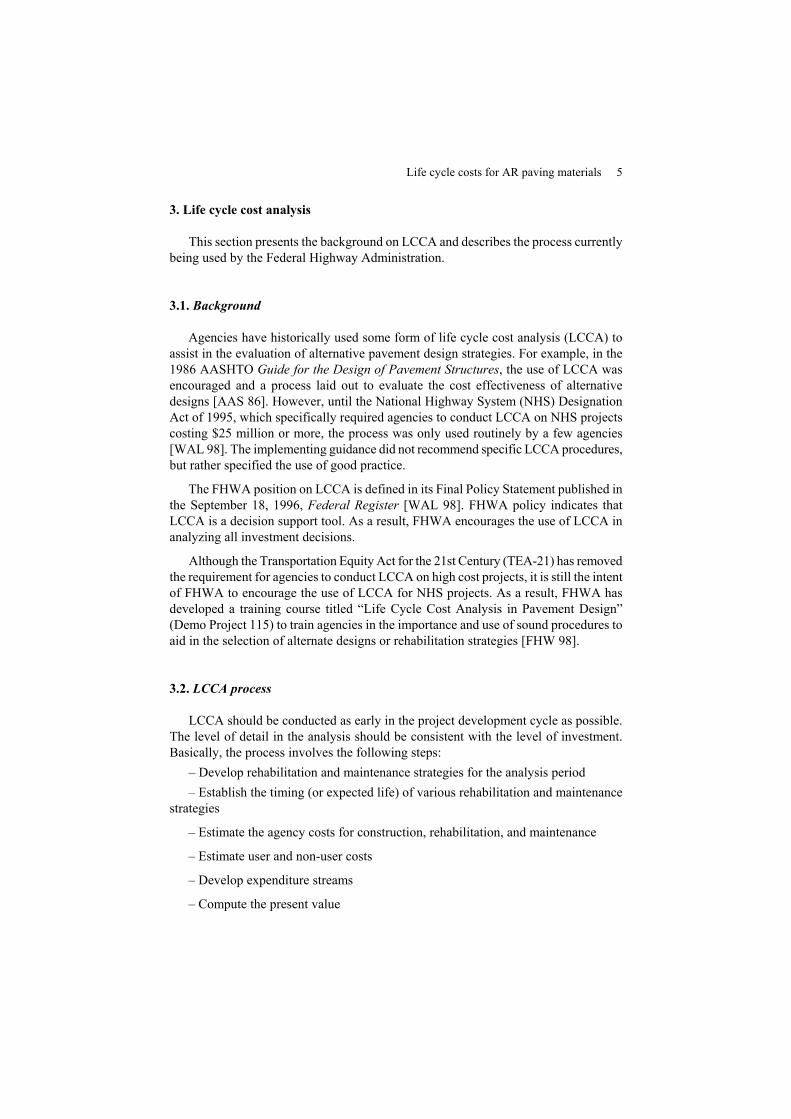
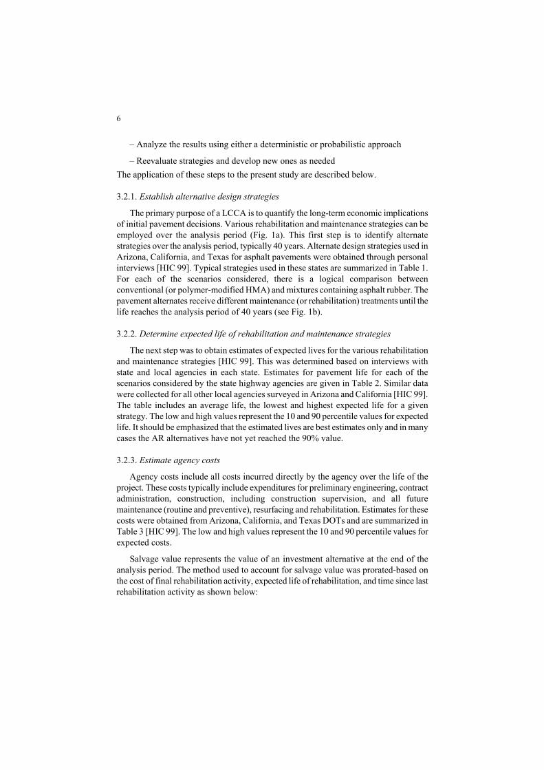
The primary purpose of a LCCA is to quantify the long-term economic implications of initial pavement decisions. Various rehabilitation and maintenance strategies can be employed over the analysis period (Fig. 1a). This first step is to identify alternate strategies over the analysis period, typically 40 years. Alternate design strategies used in Arizona, California, and Texas for asphalt pavements were obtained through personal interviews [HIC 99]. Typical strategies used in these states are summarized in Table 1. For each of the scenarios considered, there is a logical comparison between conventional (or polymer-modified HMA) and mixtures containing asphalt rubber. The pavement alternates receive different maintenance (or rehabilitation) treatments until the life reaches the analysis period of 40 years (see Fig. 1b). 3.2.2. Determine expected life of rehabilitation and maintenance strategies

The next step was to obtain estimates of expected lives for the various rehabilitation and maintenance strategies [HIC 99]. This was determined based on interviews with state and local agencies in each state. Estimates for pavement life for each of the scenarios considered by the state highway agencies are given in Table 2. Similar data were collected for all other local agencies surveyed in Arizona and California [HIC 99]. The table includes an average life, the lowest and highest expected life for a given strategy. The low and high values represent the 10 and 90 percentile values for expected life. It should be emphasized that the estimated lives are best estimates only and in many cases the AR alternatives have not yet reached the 90% value. 3.2.3. Estimate agency costs

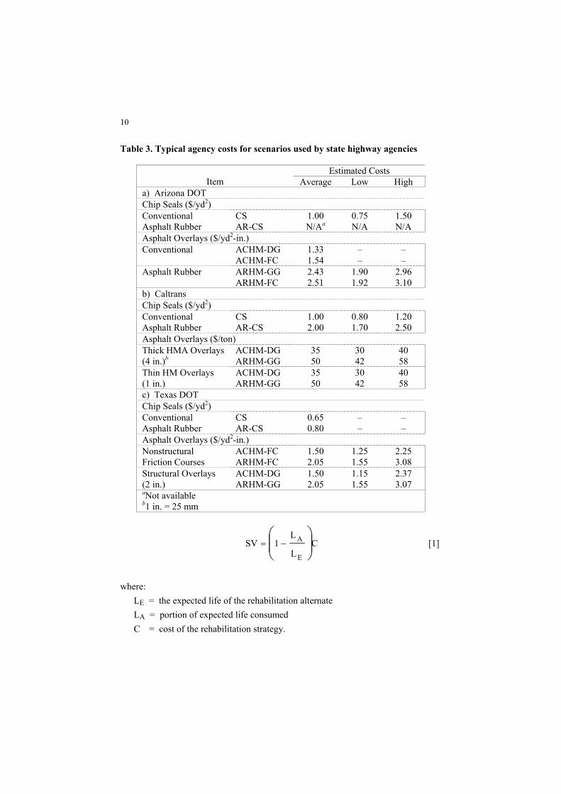
Agency costs include all costs incurred directly by the agency over the life of the project. These costs typically include expenditures for preliminary engineering, contract administration, construction, including construction supervision, and all future maintenance (routine and preventive), resurfacing and rehabilitation. Estimates for these costs were obtained from Arizona, California, and Texas DOTs and are summarized in Table 3 [HIC 99]. The low and high values represent the 10 and 90 percentile values for expected costs.

Salvage value represents the value of an investment alternative at the end of the analysis period. The method used to account for salvage value was prorated-based on the cost of final rehabilitation activity, expected life of rehabilitation, and time since last rehabilitation activity as shown below:


a) Analysis period for a pavement design alternative

b) Performance curves for two rehabilitation or maintenance strategies

Figure 1. Performance curves for two rehabilitation or maintenance strategies

8

Table 1. Typical design strategies used

Traffic Volume

Type of Activity

Existing Pavement Surface Description of Alternativesa

a) Arizona DOT Nonstructural HMA A

B C D

2.5 in. ACHM-DG + 5/8 in. ACHM-FC 2.5 in. ACHM-DG + 5/8 in. ARHM-FC 4.0 in. Mill & Fill ACHM-DG + 5/8 in. ACHM-FC 4.0 in. Mill & Fill ACHM-DG + 5/8 in. ARHM-FC

High

Structural E F

4.0 in. Mill & Fill ACHM-DG + 2.5 in. ACHM-DG + 5/8 in. ACHM-FC 4.0 in. Mill & Fill ACHM-DG + 2.5 in ARHM-GG + 5/8 in. ARHM-FC

Low Nonstructural HMA G H I

5/8 in. ACHM-FC 5/8 in. ARHM-FC 2.25 in. ACHM-DG

Nonstructural PCC J K

1 in. ARHM-FC No acceptable alternate except reconstruct

High

Structural PCC L M

Crack & Seat + 3 in. ACHM-DG + 2 in. ARHM-GG + 5/8 in. ARHM-FC Crack & Seat + 8 in. ACHM-DG

b) Caltrans Headquarters High Structural

Overlay HM A

B 4 in. ACHM-DG 2 in. ARHM-GG

Moderate Preservation Thin HMA

HMA C D

1 in. ACHM-OG 1 in. ARHM-OG

Low Chip Seal HMA E F

CS + Mill & Fill AR-CS + Mill & Fill

District 2 High Structural

Overlay G

H 4 in. ACHM-DG 2 in. ARHM-GG

High Structural Overlay

I J

4 in. ACHM-DG 2 in. ARHM-GG

Low Preservation K L

2.5 in. ACHM-DG 1.5 in. ARHM-GG

aACHM-DG = conventional hot mix – dense-graded ACHM-FC = conventional hot mix – friction course ARHM-GG = asphalt rubber hot mix – gap-graded PM-CS = polymer modified chip seal AR-CS = asphalt rubber chip seal ARHM-OG = asphalt rubber hot mix – open-graded ARHM-FC = asphalt rubber hot mix – friction course CS = chip seal b1 inch = 25 mm


Table 1. Typical design strategies used (continued)

Traffic Volume

Type of Activity

Existing Pavement Surface Description of Alternativesa

c) Texas DOT Structural HMA A

B C D

2.0 in ACHM-DG 2.0 in ACHM-GG 2.0 in. PMHM-GG 2.0 in ARHM-GG

High

Nonstructural HMA E F G

0.75 in. ACHM-FC 0.75 in. PMHM-FC 0.75 in. ARHM-FC

Nonstructural HMA H I J

AC-CS PM-CS AR-CS

Moderate

Structural HMA K L

1.5 in. ACHM-DG 1.5 in. ARHM-GG

Table 2. Typical lives for various maintenance and rehabilitation strategies, state highway agencies only

Expected Life, Years

Strategy Average

X̄ Low

L High

H a) Arizona DOT Structural Overlay Conventional

Asphalt Rubber 16 18

10 10

21 23

Thin Overlay ACHM-FC ARHM-FC

9 14

4.5 8

12 20

b) California DOT Chip Seals Conventional

Asphalt Rubber 5 7

3 3

7 12

Structural Overlay 100 mm ACHM-DG 50 mm ARHM-GG

10 10

3 4

12 12

Thin Overlay ACHM-OG ARHM-OG

10 10

5 5

12 15

c) Texas DOT Chip Seals Conventional

Asphalt Rubber 7

10 3 1

10 15

Structural Overlay 50 mm ACHM-DG 50 mm ARHM-GG

7.5 12

5 5

12 15

Thin Overlay 14 mm ACHM-FC 14 mm ARHM-FC

6.5 12

4 10

8.5 15

10

Table 3. Typical agency costs for scenarios used by state highway agencies

Estimated Costs Item Average Low High

a) Arizona DOT Chip Seals ($/yd2) Conventional Asphalt Rubber

CS AR-CS

1.00 N/Aa

0.75 N/A

1.50 N/A

Asphalt Overlays ($/yd2-in.) Conventional ACHM-DG

ACHM-FC 1.33 1.54

– –

– –

Asphalt Rubber ARHM-GG ARHM-FC

2.43 2.51

1.90 1.92

2.96 3.10

b) Caltrans Chip Seals ($/yd2) Conventional Asphalt Rubber

CS AR-CS

1.00 2.00

0.80 1.70

1.20 2.50

Asphalt Overlays ($/ton) Thick HMA Overlays (4 in.)b

ACHM-DG ARHM-GG

35 50

30 42

40 58

Thin HM Overlays (1 in.)

ACHM-DG ARHM-GG

35 50

30 42

40 58

c) Texas DOT Chip Seals ($/yd2) Conventional Asphalt Rubber

CS AR-CS

0.65 0.80

– –

– –

Asphalt Overlays ($/yd2-in.) Nonstructural Friction Courses

ACHM-FC ARHM-FC

1.50 2.05

1.25 1.55

2.25 3.08

Structural Overlays (2 in.)

ACHM-DG ARHM-GG

1.50 2.05

1.15 1.55

2.37 3.07

aNot available b1 in. = 25 mm

CL

L1SV

E

A

−= [1]

where:

LE = the expected life of the rehabilitation alternate LA = portion of expected life consumed C = cost of the rehabilitation strategy.


3.2.4. Estimate user and non-user costs

In simple terms, user costs are those incurred by the highway user over the life of the project. They include vehicle operating costs (VOC), user delay costs, and accident costs. For most pavements on the National Highway System (NHS), the VOC are considered to be similar for the different alternatives. However, slight differences in VOC rates caused by differences in roughness could result in huge differences in VOC over the life of the pavement. For purposes of this paper, VOC rates are assumed to be equal.

Delay cost rates have been derived for both passenger cars and trucks. These can range from $10-13/veh-hr for passengers cars and $17-24/veh-hr for trucks [WAL 98]. Because these costs require project specific information for inclusion in LCCA and the value of delay costs is often questioned, the authors opted to use a simpler approach using lane rental fees. Typical values for lane rental feels might vary with traffic volume as follows [HIC 99]:

Type of Facility $/Lane-Mile/Day Low volume 1,000 Moderate volume 5,000 High volume 10,000

These values are estimates only, but allow the effect of delays to be accounted for indirectly.

Accident and non-user costs may also vary with type of rehabilitation and maintenance strategy. For purposes of this paper, the effect of pavement strategy on these costs were ignored. 3.2.5. Develop expenditure streams

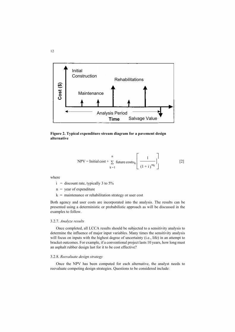
Expenditure streams are graphical or tabular representations of expenditures over time. They are generally developed for each pavement design strategy to visualize the extent and timing of expenditures. Figure 2 is an example of an expenditure stream. Normally, costs are depicted as upward arrows and benefits are reported as negative cost (or downward arrows). The only benefits, or negative cost, included herein are the costs associated with the salvage value. 3.2.6. Compute net present value (NPV)

LCCA is a form of economic analysis used to evaluate the cost efficiency of various investment options. Once all costs and their timing have been established, the future costs must be discounted to the base year and added to the initial cost to determine net present value (NPV). NPV is calculated as follows:

12

Maintenance

Rehabilitations

InitialConstruction

Cos

t ($)

TimeAnalysis Period

Salvage Value

Figure 2. Typical expenditure stream diagram for a pavement design alternative

∑

)i+(1

1 costs future +cost Initial = NPV

nkk

n

1=k

[2]

where

i = discount rate, typically 3 to 5% n = year of expenditure k = maintenance or rehabilitation strategy or user cost

Both agency and user costs are incorporated into the analysis. The results can be presented using a deterministic or probabilistic approach as will be discussed in the examples to follow. 3.2.7. Analyze results

Once completed, all LCCA results should be subjected to a sensitivity analysis to determine the influence of major input variables. Many times the sensitivity analysis will focus on inputs with the highest degree of uncertainty (i.e., life) in an attempt to bracket outcomes. For example, if a conventional project lasts 10 years, how long must an asphalt rubber design last for it to be cost effective? 3.2.8. Reevaluate design strategy

Once the NPV has been computed for each alternative, the analyst needs to reevaluate competing design strategies. Questions to be considered include:


– Are the design lives and maintenance and rehabilitation costs appropriate? – Have all costs been considered (e.g., shoulder and guard rail)? – Has uncertainty been adequately treated? – Are there other alternates which should be considered?

Many assumptions, estimates, and projections feed the LCCA process. The variability associated with these inputs can have a major influence on the results. 4. LCCA examples

The life cycle cost analysis calculations presented herein were completed using a combination of two widely available software programs, MicroSoft Excel (deterministic) and Palisades’ @Risk (probabilistic) as suggested by the Federal Highway Administration [WAL 98]. This combination allows both the deterministic and probabilistic approaches to be analyzed. Before describing the scenarios investigated, an overview of the general features of each is described along with the assumptions. 4.1. Scenario overview

Several features were common to each analysis. These are described below: – A 40-year analysis period was selected based on FHWA recommendations (5). – Each major rehabilitation activity triggered a lane rental cost calculated as a

function of the production rate assumed for that traffic level/facility type. – Routine maintenance may be applied between major rehabilitation activities

depending on the agency. – Salvage values were calculated as a prorated percentage of the expected life of the

rehabilitation. – All costs were converted to present worth terms to compare asphalt rubber and

non-asphalt rubber alternatives. In addition, several assumptions and simplifications were necessary. These are listed below:

– Maintenance was applied as indicated by the agency. Once triggered, maintenance costs occur until the next major rehabilitation activity.

– User delay costs were approximated using the lane rental costs. The authors recognize that more accurate costs could be determined if actual average daily traffic (ADT) were known (or assumed) and delays were computed; however, this was beyond the scope of this project. Several input were consistent among all different scenarios are shown in Table 4.

14

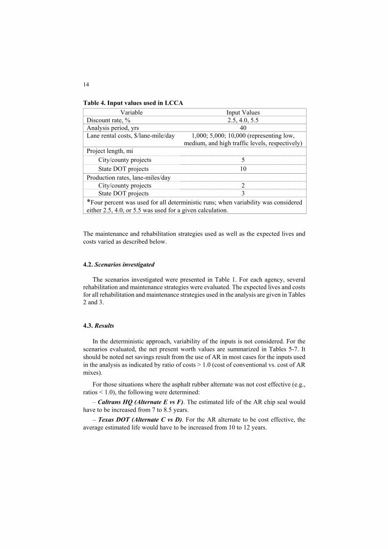
Table 4. Input values used in LCCA Variable Input Values

Discount rate, % 2.5, 4.0, 5.5 Analysis period, yrs 40 Lane rental costs, $/lane-mile/day 1,000; 5,000; 10,000 (representing low,

medium, and high traffic levels, respectively) Project length, mi

City/county projects 5 State DOT projects 10

Production rates, lane-miles/day City/county projects 2 State DOT projects 3

*Four percent was used for all deterministic runs; when variability was considered either 2.5, 4.0, or 5.5 was used for a given calculation.

The maintenance and rehabilitation strategies used as well as the expected lives and costs varied as described below. 4.2. Scenarios investigated

The scenarios investigated were presented in Table 1. For each agency, several rehabilitation and maintenance strategies were evaluated. The expected lives and costs for all rehabilitation and maintenance strategies used in the analysis are given in Tables 2 and 3. 4.3. Results

In the deterministic approach, variability of the inputs is not considered. For the scenarios evaluated, the net present worth values are summarized in Tables 5-7. It should be noted net savings result from the use of AR in most cases for the inputs used in the analysis as indicated by ratio of costs > 1.0 (cost of conventional vs. cost of AR mixes).

For those situations where the asphalt rubber alternate was not cost effective (e.g., ratios < 1.0), the following were determined:

– Caltrans HQ (Alternate E vs F). The estimated life of the AR chip seal would have to be increased from 7 to 8.5 years.

– Texas DOT (Alternate C vs D). For the AR alternate to be cost effective, the average estimated life would have to be increased from 10 to 12 years.

18

– Texas DOT (Alternate I vs J). For the AR alternate to be cost effective, the average estimated life would have to be increased from 9 to 12 years.

– Texas DOT (Alternate H vs J). For the AR alternate to be cost effective, the average expected life would have to be increased from 9 to 16 years. It should be emphasized that all of the estimates lives are best estimates provided by the agencies. Any change in estimated life can have a significant effect on the LCCA.

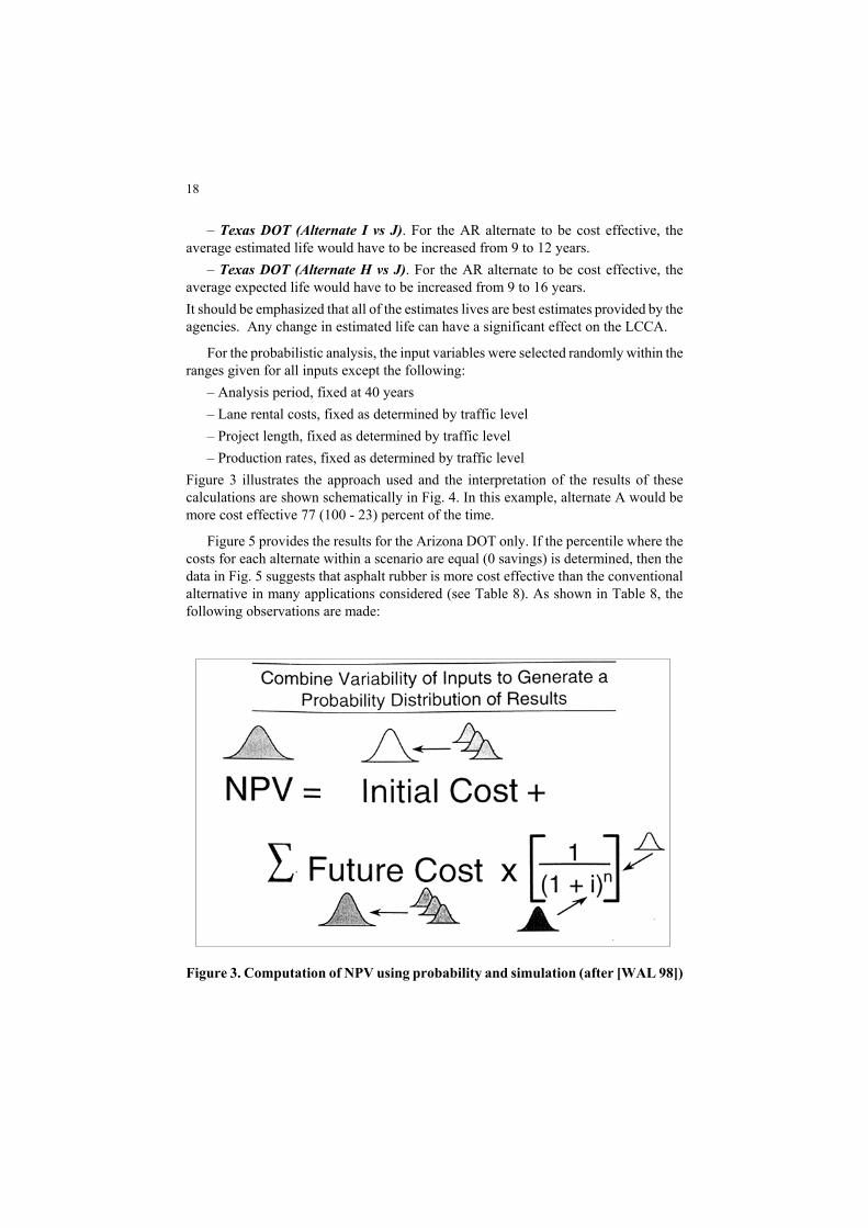
For the probabilistic analysis, the input variables were selected randomly within the ranges given for all inputs except the following:

– Analysis period, fixed at 40 years – Lane rental costs, fixed as determined by traffic level – Project length, fixed as determined by traffic level – Production rates, fixed as determined by traffic level

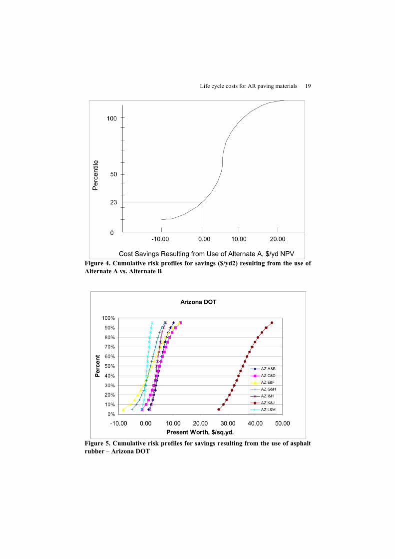
Figure 3 illustrates the approach used and the interpretation of the results of these calculations are shown schematically in Fig. 4. In this example, alternate A would be more cost effective 77 (100 - 23) percent of the time.

Figure 5 provides the results for the Arizona DOT only. If the percentile where the costs for each alternate within a scenario are equal (0 savings) is determined, then the data in Fig. 5 suggests that asphalt rubber is more cost effective than the conventional alternative in many applications considered (see Table 8). As shown in Table 8, the following observations are made:

Figure 3. Computation of NPV using probability and simulation (after [WAL 98])

Life cycle costs for AR paving materials 19 Pe

rcen

tile

Cost Savings Resulting from Use of Alternate A, $/yd NPV

0

23

50

100

-10.00 0.00 10.00 20.00

Figure 4. Cumulative risk profiles for savings ($/yd2) resulting from the use of Alternate A vs. Alternate B

Arizona DOT

0%

10%

20%

30%

40%

50%

60%

70%

80%

90%

100%

-10.00 0.00 10.00 20.00 30.00 40.00 50.00Present Worth, $/sq.yd.

Perc

ent

AZ A&B

AZ C&D

AZ E&F

AZ G&H

AZ I&H

AZ K&J

AZ L&M

Figure 5. Cumulative risk profiles for savings resulting from the use of asphalt rubber – Arizona DOT

20

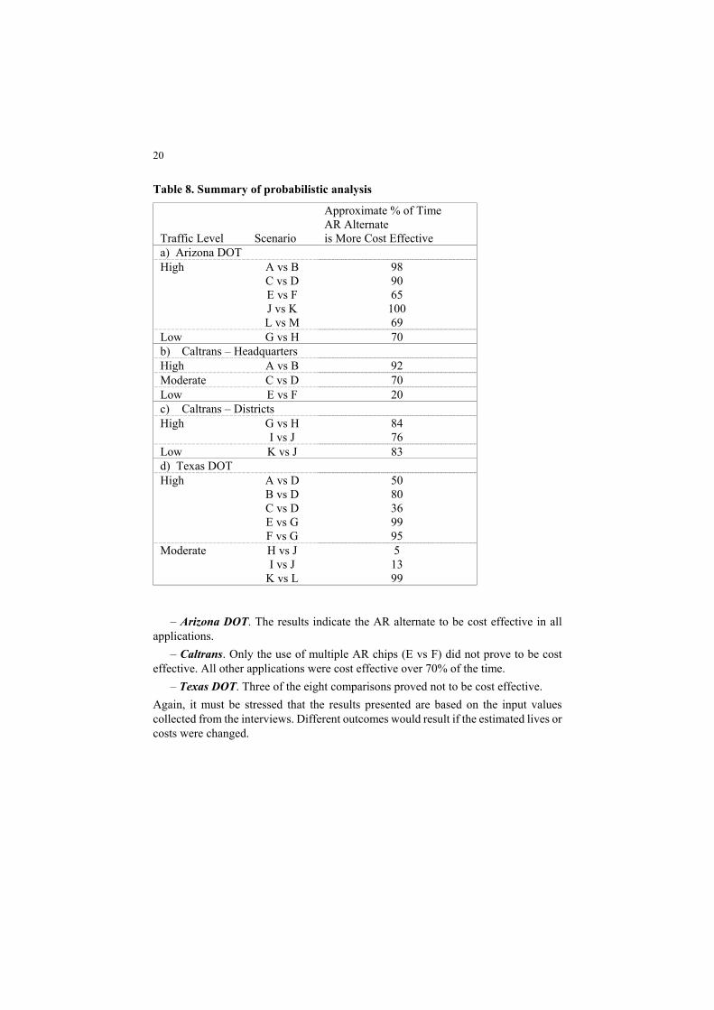
Table 8. Summary of probabilistic analysis

Traffic Level Scenario

Approximate % of Time AR Alternate is More Cost Effective

a) Arizona DOT High A vs B

C vs D E vs F J vs K L vs M

98 90 65

100 69

Low G vs H 70 b) Caltrans – Headquarters High A vs B 92 Moderate C vs D 70 Low E vs F 20 c) Caltrans – Districts High G vs H

I vs J 84 76

Low K vs J 83 d) Texas DOT High A vs D

B vs D C vs D E vs G F vs G

50 80 36 99 95

Moderate H vs J I vs J

K vs L

5 13 99

– Arizona DOT. The results indicate the AR alternate to be cost effective in all applications.

– Caltrans. Only the use of multiple AR chips (E vs F) did not prove to be cost effective. All other applications were cost effective over 70% of the time.

– Texas DOT. Three of the eight comparisons proved not to be cost effective. Again, it must be stressed that the results presented are based on the input values collected from the interviews. Different outcomes would result if the estimated lives or costs were changed.


4.4. Guidelines for use Asphalt rubber is cost effective for most of the scenarios presented in this report. LCCA should be used to evaluate alternate maintenance and rehabilitation strategies to answer the following questions:

– Where to use asphalt rubber? Can asphalt rubber be used on the existing pavement types (HMA, PCC) and in the environmental conditions present at the site? Based on the results of this study, the use of asphalt rubber products is a cost effective solution in most of the scenarios evaluated.

– What asphalt rubber products to use? Both AR hot-mix and/or chip seals proved to be cost effective for the intended applications. Allowing a thickness reduction increases the cost effectiveness of asphalt-rubber hot-mix applications.

– When to use asphalt rubber? Historically, AR was often used on only the poorest pavements. The results of this study suggest they can be used for all pavement conditions but are most cost effective when reflection cracking is expected [WAY 98].

– What is the user cost impact? Is it significantly different between the scenarios investigated? The differences in user costs between the conventional and AR alternates was not great. This is likely due to the fact that the user costs employed were related to low to medium volume traffic conditions. For high volume urban facilities, the differences in user costs would likely be greater. It should be emphasized that asphalt rubber binders will not be cost effective unless the thickness of the layer is reduced or extended life is achieved. 5. Conclusions and recommendations 5.1. Conclusions

Based on the information provided by the agencies and the results of the analyses, the following conclusions are warranted:

– For the scenarios evaluated, asphalt rubber is a cost effective alternate for many highway pavement applications.

– When variability is considered in the inputs (cost, expected life, etc.), the asphalt rubber alternates would be the best choice in most of the applications considered.

– Asphalt rubber was not cost effective in all applications. LCCA allows one to determine when and where AR will be cost effective. The results of LCCA are highly dependent on the input variables. Many times these inputs are only best estimates. Every effort is needed to obtain accurate estimates of the average value and expected variability for each input variable. Further, the cost effectiveness of AR is dependent in many of the cases on the ability to reduce thickness when using AR. Without a reduction in thickness, or longer lives for equal thicknesses, the AR alternates would not be cost effective.

22

5.2. Recommendations

Agencies which intend to use asphalt rubber need to consider performing a life cycle cost analysis to determine whether a proposed application is cost effective. As demonstrated in this report, asphalt rubber may not be cost effective for all operations.

A limitation of this study is the lack of good long-term performance data for comparative sections of conventional, polymer modified, and asphalt rubber mixtures. The FHWA pooled fund study, designed to provide this sort of data, was stopped in 1997. This information is still needed if LCCA comparisons between alternates are to be made.

6. References [AAS 86] AASHTO, Guide for design of pavement structures, American Association of State

Highway and Transportation Officials, 1986.

[EPP 94] EPPS J.A., “Uses of recycled rubber tires in highways,” NCHRP synthesis 198, TRB, National Research Council, Washington, DC, 1994, 162 p.

[FHW 98] FHWA, Life cycle cost analysis in pavement design demonstration Project 115 – participant notebook, FHWA-SA-98-400, FHWA, August 1998.

[HIC 95] HICKS R.G., LUNDY J.R., LEAHY R.B., HANSON D., EPPS J.A., Crumb rubber modifiers (CRM) in asphalt pavements: summary of practices in Arizona, California and Florida, Report FHWA-SA-95-056, FHWA, September 1995.

[HIC 99] HICKS R.G., LUNDY J.R., EPPS J.A. Life cycle costs for asphalt-rubber paving materials, Final Report to Rubber Pavements Association, vols. I/II, June 1999.

[SCO 89] SCOFIELD L.A., The history, development and performance of asphalt rubber at ADOT, Report AZ-SP-8902, Arizona Transportation Research Center, Arizona Department of Transportation, December 1989.

[WAL 98] WALLS J., SMITH M.R., Life cycle cost analysis in pavement design, Report FHWA-SA-98-079, FHWA, September 1998.

[WAY 98] WAY G.B., “OGFC meetings CRM – where the rubber meets the rubber,” presented at the Asphalt Conference, Atlanta, GA, March 1998.

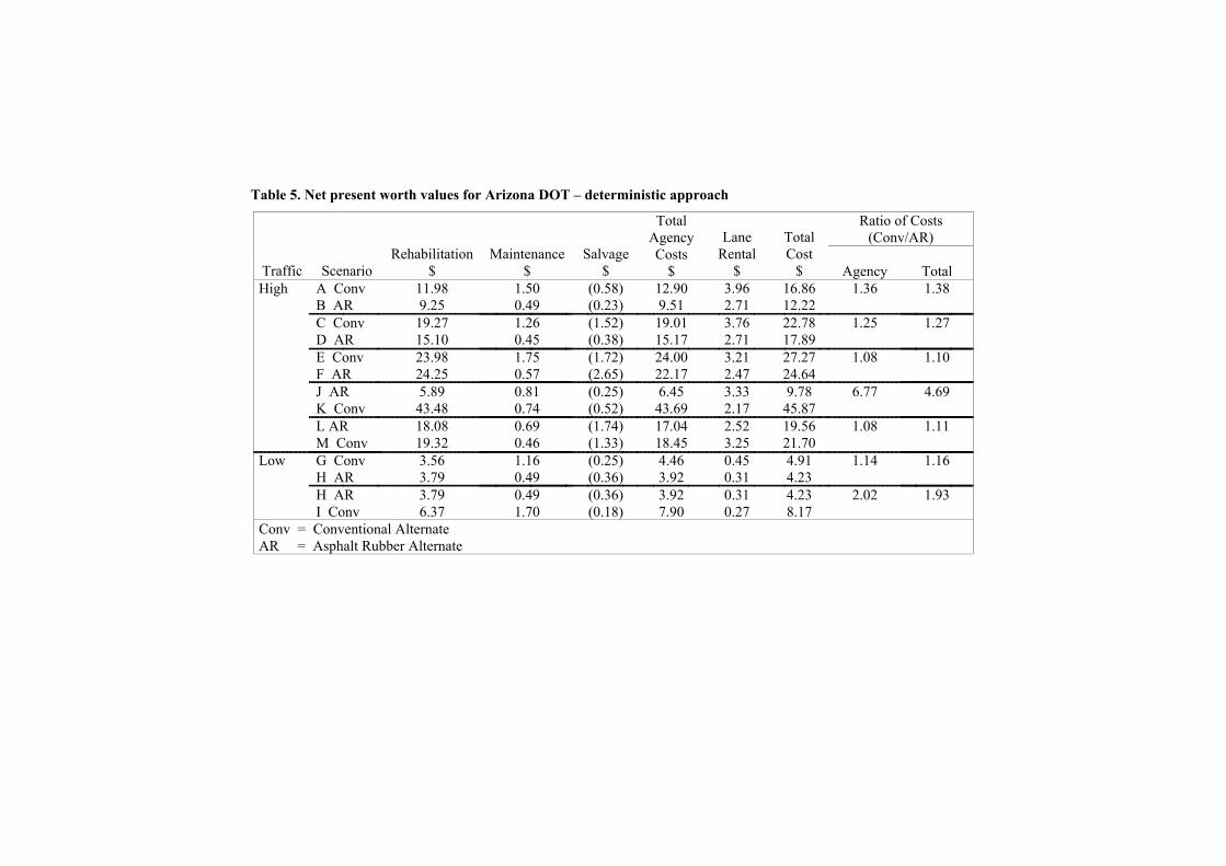
Table 5. Net present worth values for Arizona DOT – deterministic approach

Ratio of Costs (Conv/AR)

Traffic ScenarioRehabilitation

$ Maintenance

$ Salvage

$

Total Agency Costs

$

Lane Rental

$

Total Cost

$ Agency TotalA Conv B AR

11.98 9.25

1.50 0.49

(0.58) (0.23)

12.90 9.51

3.96 2.71

16.86 12.22

1.36 1.38

C Conv D AR

19.27 15.10

1.26 0.45

(1.52) (0.38)

19.01 15.17

3.76 2.71

22.78 17.89

1.25 1.27

E Conv F AR

23.98 24.25

1.75 0.57

(1.72) (2.65)

24.00 22.17

3.21 2.47

27.27 24.64

1.08 1.10

J AR K Conv

5.89 43.48

0.81 0.74

(0.25) (0.52)

6.45 43.69

3.33 2.17

9.78 45.87

6.77 4.69

High

L AR M Conv

18.08 19.32

0.69 0.46

(1.74) (1.33)

17.04 18.45

2.52 3.25

19.56 21.70

1.08 1.11

G Conv H AR

3.56 3.79

1.16 0.49

(0.25) (0.36)

4.46 3.92

0.45 0.31

4.91 4.23

1.14 1.16Low

H AR I Conv

3.79 6.37

0.49 1.70

(0.36) (0.18)

3.92 7.90

0.31 0.27

4.23 8.17

2.02 1.93

Conv = Conventional Alternate AR = Asphalt Rubber Alternate

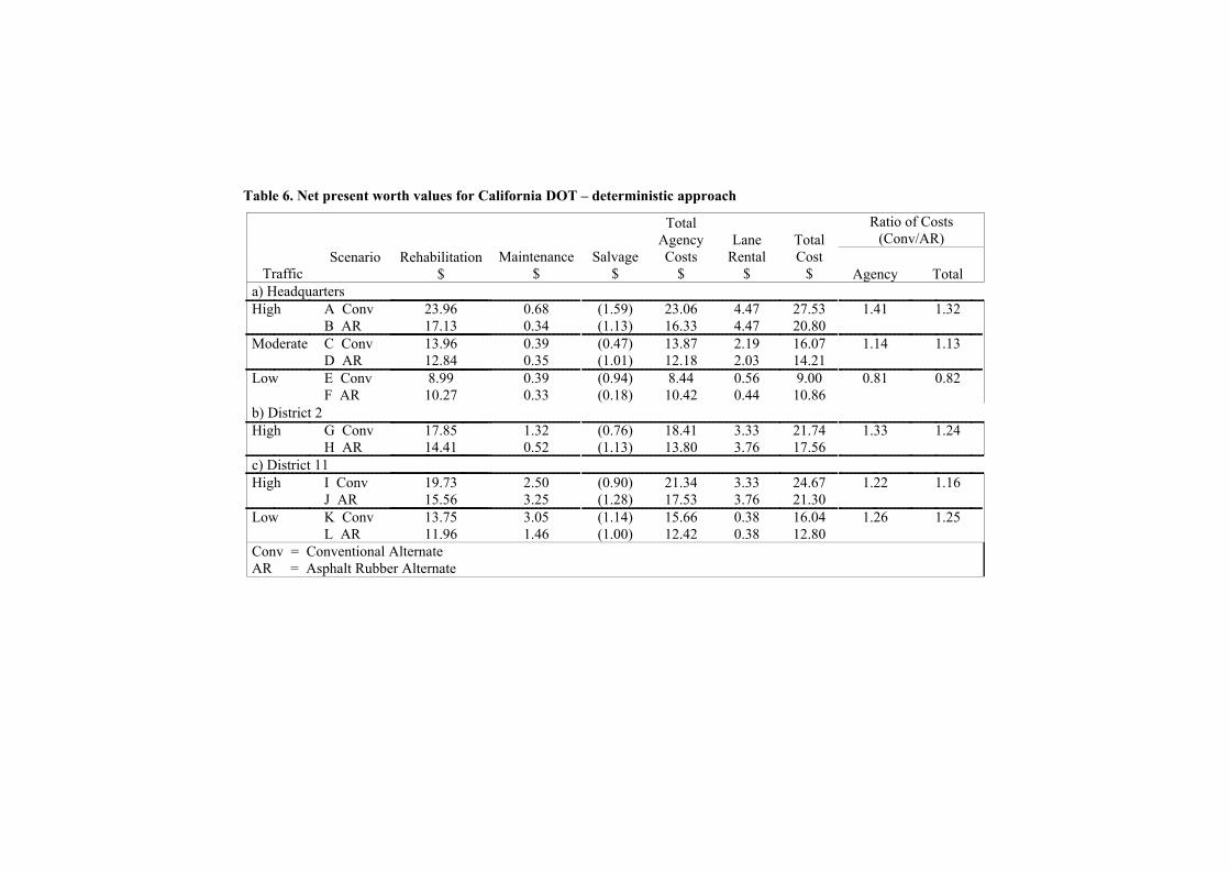
Table 6. Net present worth values for California DOT – deterministic approach

Ratio of Costs

(Conv/AR)

Traffic Scenario

Rehabilitation

$ Maintenance

$ Salvage

$

Total Agency Costs

$

Lane Rental

$

Total Cost

$ Agency Totala) Headquarters High A Conv

B AR 23.96 17.13

0.68 0.34

(1.59) (1.13)

23.06 16.33

4.47 4.47

27.53 20.80

1.41 1.32

Moderate C Conv D AR

13.96 12.84

0.39 0.35

(0.47) (1.01)

13.87 12.18

2.19 2.03

16.07 14.21

1.14 1.13

Low E Conv F AR

8.99 10.27

0.39 0.33

(0.94) (0.18)

8.44 10.42

0.56 0.44

9.00 10.86

0.81 0.82

b) District 2 High G Conv

H AR 17.85 14.41

1.32 0.52

(0.76) (1.13)

18.41 13.80

3.33 3.76

21.74 17.56

1.33 1.24

c) District 11 High I Conv

J AR 19.73 15.56

2.50 3.25

(0.90) (1.28)

21.34 17.53

3.33 3.76

24.67 21.30

1.22 1.16

Low K Conv L AR

13.75 11.96

3.05 1.46

(1.14) (1.00)

15.66 12.42

0.38 0.38

16.04 12.80

1.26 1.25


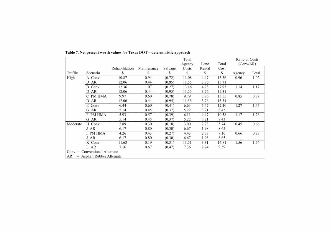
Table 7. Net present worth values for Texas DOT – deterministic approach Ratio of Costs

(Conv/AR)

Traffic ScenarioRehabilitation

$ Maintenance

$ Salvage

$

Total Agency Costs

$

Lane Rental

$

Total Cost

$ Agency TotalA Conv D AR

10.87 12.06

0.94 0.44

(0.72) (0.95)

11.08 11.55

4.47 3.76

15.56 15.31

0.96 1.02

B Conv D AR

12.36 12.06

1.07 0.44

(0.27) (0.95)

13.16 11.55

4.78 3.76

17.93 15.31

1.14 1.17

C PM HMA D AR

9.97 12.06

0.60 0.44

(0.78) (0.95)

9.79 11.55

3.76 3.76

13.55 15.31

0.85 0.89

E Conv G AR

6.44 5.14

0.60 0.45

(0.41) (0.37)

6.63 5.22

5.47 3.21

12.10 8.43

1.27 1.43

High

F PM HMA G AR

5.93 5.14

0.57 0.45

(0.39) (0.37)

6.11 5.22

4.47 3.21

10.58 8.43

1.17 1.26

H Conv J AR

2.89 6.17

0.30 0.80

(0.18) (0.30)

3.00 6.67

2.73 1.98

5.74 8.65

0.45 0.66

I PM HMA J AR

4.26 6.17

0.43 0.80

(0.27) (0.30)

4.43 6.67

2.73 1.98

7.16 8.65

0.66 0.83

Moderate

K Conv L AR

11.63 7.16

0.19 0.67

(0.31) (0.47)

11.51 7.36

3.31 2.24

14.81 9.59

1.56 1.54


life cycle costs for asphalt-rubber paving...

Documents