lie groups in physics1 institute for theoretical physics ...hooft101/lectures/lieg07.pdf · lie...
TRANSCRIPT
LIE GROUPS IN PHYSICS1
version 25/06/07
Institute for Theoretical Physics
Utrecht University
Beta Faculty
2007
English version by G. ’t Hooft
Original text by M.J.G. Veltman
B.Q.P.J. de Wit
and G. ’t Hooft
Contents
1 Introduction 1
2 Quantum mechanics and rotation invariance 7
3 The group of rotations in three dimensions 14
4 More about representations 22
5 Ladder operators 26
6 The group SU (2) 31
7 Spin and angular distributions 39
8 Isospin 45
9 The Hydrogen Atom 48
10 The group SU(3) 55
11 Representations of SU(N); Young tableaus 60
12 Beyond these notes 61
Appendix A. Summary of the properties of matrices 62
Appendix B. Differentiation of matrices 64
Appendix C. Functins of matrices 65
Appendix D. The Campbell-Baker-Hausdorff formula 66
Appendix E. Complex inner product, unitary and hermitian matrices 70
1. Introduction
Many systems studied in physics show some form of symmetry. In physics, this meansthe following: we can consider some transformation rule, like a rotation, a displacement,or the reflection by a mirror, and we compare the original system with the transformedsystem. If they show some resemblance, we have a symmetry. A snow flake looks likeitself when we rotate it by 60 or when we perform a mirror reflection. We say thatthe snow flake has a symmetry. If we replace a proton by a neutron, and vice versa, thereplaced particles behave very much like the originals; this is also a symmetry. Many lawsof Nature have symmetries in this sense. Sometimes the symmetry is perfect, but oftenit is not exact; the transformed system is then slightly different from the original; thesymmetry is broken.
If system A resembles system B , and system B resembles C , then A resemblesC . Therefore, the product of two symmetry transformations is again a symmetry trans-formation. Thus, the set of all symmetry transformations that characterize the symmetryof a system, are elements of a group. For example, the reflections with respect to a planeform a group that contains just two elements: the reflection operation and the identity— the identity being the one operation that leaves everything the same. The rotations inthree-dimensional space, the set of all Lorentz transformations, and the set of all paralleldisplacements also form groups, which have an unlimited number of elements. For obvi-ous reasons, groups with a finite (or denumerable) number of elements are called discretegroups; groups of transformations that continuously depend on a number of parameters,such as the rotations, which can be defined in terms of a few angular parameters, arecalled continuous groups.
The symmetry of a system implies certain relations among observable quantities, whichmay be obeyed with great precision, independently of the nature of the forces acting in thesystem. In the hydrogen atom, for example, one finds that the energies of different statesof the atom, are exactly equal, as a consequence of the rotational invariance of the system.However, one also often finds that the symmetry of a physical system is only approximatelyrealized. An infinite crystal, for example, is invariant under those translations for whichthe displacement is an integral multiple of the distance between two adjacent atoms. Inreality, however, the crystal has a definite size, and its surface perturbs the translationalsymmetry. Nevertheless, if the crystal contains a sufficiently large number of atoms, thedisturbance due to the surface has little effects on the properties at the interior.
An other example of a symmetry that is only approximately realized, is encounteredin elementary particle physics. The so-called ∆+ particle, which is one of the excitedstates of the nucleons, decays into a nucleon and an other particle, the π -meson, alsocalled pion. There exist two kinds of nucleons, neutrons and protons, and there are threetypes of pions, the electrically charged pions π+ and π− , and the neutral one, π0 . Sincethe total electric charge of the ∆+ must be preserved during its decay, one distinguishes
1This lecture course was originally set up by M. Veltman, and subsequently modified and extendedby B. de Wit and G. ’t Hooft.
1
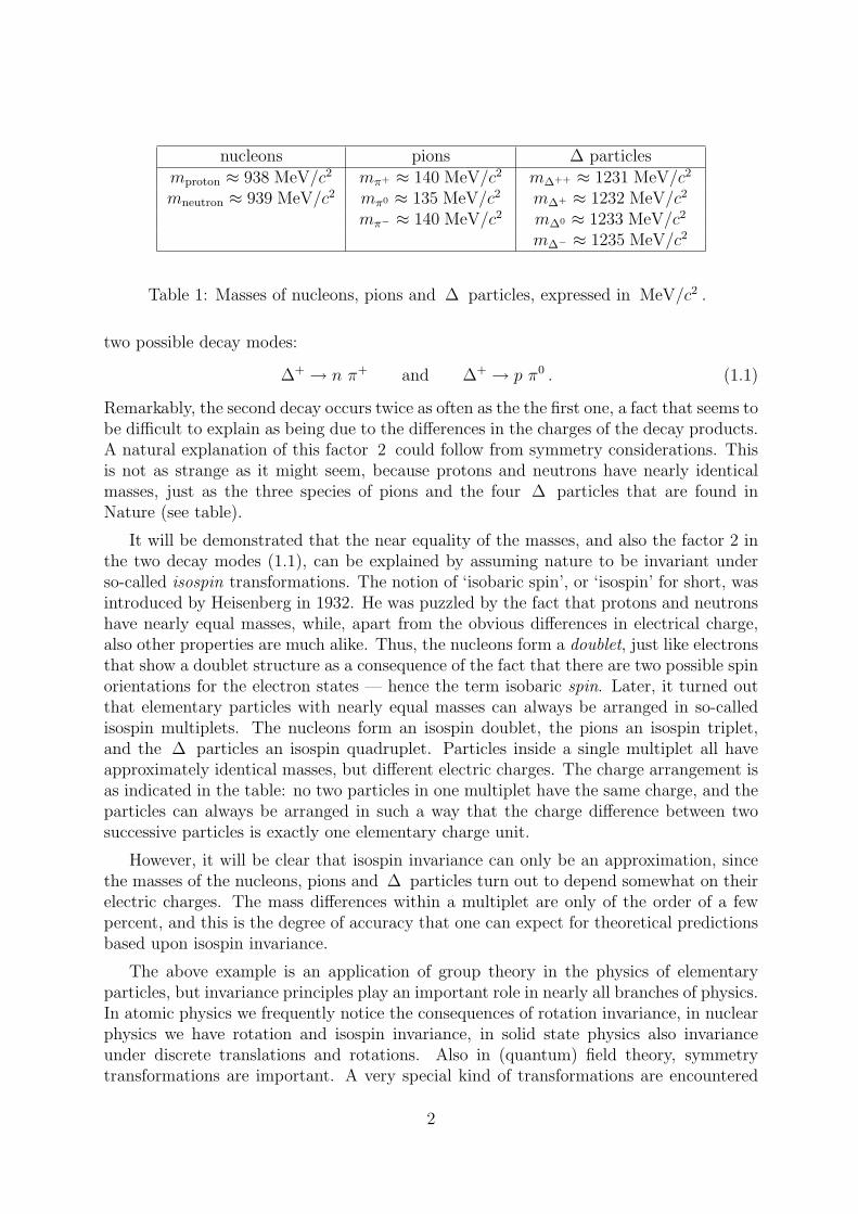
nucleons pions ∆ particlesmproton ≈ 938 MeV/c2 mπ+ ≈ 140 MeV/c2 m∆++ ≈ 1231 MeV/c2
mneutron ≈ 939 MeV/c2 mπ0 ≈ 135 MeV/c2 m∆+ ≈ 1232 MeV/c2
mπ− ≈ 140 MeV/c2 m∆0 ≈ 1233 MeV/c2
m∆− ≈ 1235 MeV/c2
Table 1: Masses of nucleons, pions and ∆ particles, expressed in MeV/c2 .
two possible decay modes:
∆+ → n π+ and ∆+ → p π0 . (1.1)
Remarkably, the second decay occurs twice as often as the the first one, a fact that seems tobe difficult to explain as being due to the differences in the charges of the decay products.A natural explanation of this factor 2 could follow from symmetry considerations. Thisis not as strange as it might seem, because protons and neutrons have nearly identicalmasses, just as the three species of pions and the four ∆ particles that are found inNature (see table).
It will be demonstrated that the near equality of the masses, and also the factor 2 inthe two decay modes (1.1), can be explained by assuming nature to be invariant underso-called isospin transformations. The notion of ‘isobaric spin’, or ‘isospin’ for short, wasintroduced by Heisenberg in 1932. He was puzzled by the fact that protons and neutronshave nearly equal masses, while, apart from the obvious differences in electrical charge,also other properties are much alike. Thus, the nucleons form a doublet, just like electronsthat show a doublet structure as a consequence of the fact that there are two possible spinorientations for the electron states — hence the term isobaric spin. Later, it turned outthat elementary particles with nearly equal masses can always be arranged in so-calledisospin multiplets. The nucleons form an isospin doublet, the pions an isospin triplet,and the ∆ particles an isospin quadruplet. Particles inside a single multiplet all haveapproximately identical masses, but different electric charges. The charge arrangement isas indicated in the table: no two particles in one multiplet have the same charge, and theparticles can always be arranged in such a way that the charge difference between twosuccessive particles is exactly one elementary charge unit.
However, it will be clear that isospin invariance can only be an approximation, sincethe masses of the nucleons, pions and ∆ particles turn out to depend somewhat on theirelectric charges. The mass differences within a multiplet are only of the order of a fewpercent, and this is the degree of accuracy that one can expect for theoretical predictionsbased upon isospin invariance.
The above example is an application of group theory in the physics of elementaryparticles, but invariance principles play an important role in nearly all branches of physics.In atomic physics we frequently notice the consequences of rotation invariance, in nuclearphysics we have rotation and isospin invariance, in solid state physics also invarianceunder discrete translations and rotations. Also in (quantum) field theory, symmetrytransformations are important. A very special kind of transformations are encountered
2
for example in electrodynamics. Here, electric and magnetic fields can be expressed interms of the so-called vector potential Aµ(x) , for which we use a relativistic four-vectornotation ( µ = 0, 1, 2, 3 ):
Aµ(x) = (− c−1 φ(x), A(x)) , xµ = (ct, x) , (1.2)
where φ denotes the potential, and A the three-dimensional vector potential field; c isthe velocity of light. The electric and magnetic fields are defined by
E = −∇φ− c−1 ∂A
∂t, (1.3)
B = ∇×A . (1.4)
An electrically charged particle is described by a complex wave function ψ(~x, t) . TheSchrodinger equation obeyed by this wave function remains valid when one performs arotation in the complex plane:
ψ(~x, t) → eiΛ ψ(~x, t) . (1.5)
Is the phase factor Λ allowed to vary in space and time?
The answer to this is yes, however only if the Schrodinger equation depends on thevector potential in a very special way. Wherever a derivative ∂µ occurs, it must be inthe combination
Dµ = ∂µ − ieAµ , (1.6)
where e is the electric charge of the particle in question. If Λ(~x, t) depends on ~x andt , then (1.5) must be associated with the following transformation rules for the potentialfields:
A(x) → A(x) + e−1∇Λ(x) , (1.7)
φ(x) → φ(x)− (c e)−1 ∂
∂tΛ(x) , (1.8)
or, in four-vector notation,
Aµ(x) → Aµ(x) + e−1∂µΛ(x) . (1.9)
It can now easily be established that E en B will not be affected by this so-calledgauge transformation. Furthermore, we derive:
Dµψ(x) → eiΛ(x)Dµψ(x) . (1.10)
Notice that the substitution (1.6) in the Schrodinger equation is all that is needed toinclude the interaction of a charged particle with the fields E en B .
These phase factors define a group, called the group of 1× 1 unitary matrices, U(1) .In this case, the group is quite a simple one, but it so happens that similar theories exist
3
that are based on other (continuous) groups that are quite a bit more complicated such asthe group SU(2) that will be considered in these lectures. Theories of this type are knownas gauge theories, or Yang-Mills theories, and the field Aµ is called a gauge field. Thefact that E en B are invariant under gauge transformations implies that electromagneticphenomena are gauge-invariant. For more general groups it turns out that several of thesegauge fields are needed: they form multiplets.
Surprisingly, the theory of gravitation, Einstein’s general relativity theory, turns outto be a gauge theory as well, be it of a somewhat different type. This theory can beconsidered to be the gauge theory of the general coordinate transformations, the mostgeneral reparametrizations of points in space and time,
xµ → xµ + ξµ(x) . (1.11)
The gauge field here is the gravitational field, taking the form of a metric, which is to beused in the definitions of distances and angles in four-dimensional space and time. All ofthis is the subject of an entire lecture course, Introduction to General Relativity.
The fact that gauge transformations are associated to an abstract group, and candepend on space and time as well, can give rise to interesting phenomena of a topologicalnature. Examples of this are flux quantization in super conductors, the Aharonov-Bohmeffect in quantum mechanics, and magnetic monopoles. To illustrate the relevance oftopology, we consider again the group of the U(1) gauge transformations, but now intwo-dimensional space (or equivalently, in a situation where the fields only depend ontwo of the three space coordinates). Let ψ(x, y) be a complex function, such as a wavefunction in quantum mechanics, transforming under these gauge transformations, i.e.
ψ(x, y) → eiΛ(x,y)ψ(x, y) . (1.12)
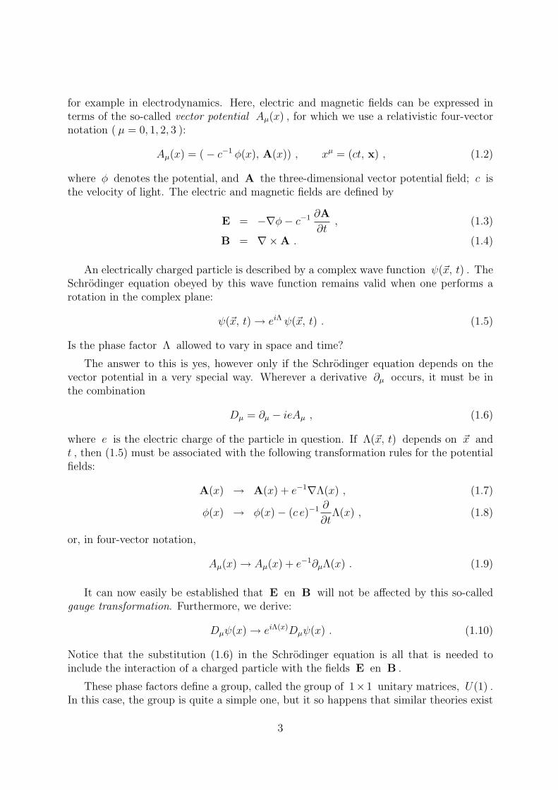
From the fact that the phase of ψ can be modified everywhere by applying differentgauge transformations, one might conclude that the phase of ψ is actually irrelevant forthe description of the system. This however is not quite the case. Consider for instancea function that vanishes at the origin. Now take a closed curve in the x - y plane, andcheck how the phase of ψ(x, y) changes along the curve. After a complete run along thecurve the phase might not necessarily take the same value as at the beginning, but if weassume that ψ(x, y) is single-valued on the plane, then the phase difference will be equalto 2πn , where n is an arbitrary integral number. This number is called the windingnumber. An example of a situation with winding number n = 1 is pictured in Fig. 1; thephase angle makes a full turn over 2π when we follow the function ψ(x, y) along a curvewinding once around the origin. One can easily imagine situations with other windingnumbers. The case n = 0 for instance occurs when the phase of ψ(x, y) is constant.
If we change the function ψ(x, y) continuously, the winding number will not change.This is why the winding number is called a topological invariant. This also implies that thewinding number will not change under the gauge transformations (1.12), provided thatwe limit ourselves to gauge transformations that are well-defined in the entire plane. Notealso that the winding number does not depend on the choice of the closed curve aroundthe origin, as long as it is not pulled across the origin or any other zero of the function
4
Figure 1: De phase angle of ψ(x, y) indicated by an arrow (whose length is immaterial,but could be given for instance by |ψ(x, y)| ) at various spots in the x - y plane. Thisfunction has a zero at the origin.
ψ(x, y) . All this implies that although locally, that is, at one point and its immediateneighborhood, the phase of ψ can be made to vanish, this can be realized globally, thatis, on the entire plane, only if the winding number for any closed curve equals zero.
A similar situation can be imagined for the vector potential. Once more considerthe two-dimensional plane, and assume that we are dealing with a magnetic field that iseverywhere equal to zero, except for a small region surrounding the origin. In this region,A cannot be equal to zero, because of the relation (1.4). However, in the surroundingregion, where B vanishes, there may seem to be no reason why not also A should vanish.Indeed, one can show that, at every given point and its neighborhood, a suitably chosengauge transformation can ensure A(x) to vanish there. This result, however, can onlyhold locally, as we can verify by considering the following loop integral:
Φ[C] =
∮
C
Ai dxi, (1.13)
where C is a given closed curve. It is easy to check that Φ[C] does not change undera gauge transformation (1.5). Indeed, we know from the theory of magnetism that Φ[C]must be proportional to the total magnetic flux through the surface enclosed by the curveC .
Applying this to the given situation, we take the curve C to surround the origin andthe region where B 6= 0 , so that the B field vanishes on the curve itself. The quantityΦ[C] equals the total flux through C , which may well be different from zero. If thisis the case, we cannot transform A away in the entire outside region, even if it canbe transformed away locally2. Note that the magnetic flux here plays the same role asthe winding number of the previous example. Indeed, in superconducting material, thegauge phases can be chosen such that A vanishes, and consequently, magnetic flux goingthrough a superconducting coil is limited to integral values: the flux is quantized.
2This causes an interesting quantum mechanical effect in electrons outside a magnetic field, to wit,the Aharonov-Bohm effect.
5
Under some circumstances, magnetic field lines can penetrate superconducting mate-rials in the form of vortices. These vortices again are quantized. In the case of more com-plicated groups, such as SU(2) , other situations of a similar nature can occur: magneticmonopoles are topologically stable objects in three dimensions; even in four dimensionsone can have such phenomena, referred to as “instantons”.
Clearly, group theory plays an essential role in physics. In these lectures we willprimarily limit ourselves to the group of three-dimensional rotations, mostly in the contextof quantum mechanics. Many of the essentials can be clarified this way, and the treatmentcan be made reasonably transparent, physically and mathematically. The course does notintend to give a complete mathematical analysis; rather, we wish to illustrate as clearly aspossible the relevance of group theory for physics. Therefore, some physical applicationswill be displayed extensively. The rotation group is an example of a so-called compact Liegroup. In most applications, we consider the representations of this group. Representationtheory for such groups is completely known in mathematics. Some advance knowledgeof linear algebra (matrices, inner products, traces, functions and derivatives of matrices,etc.) will be necessary. For completeness, some of the most important properties ofmatrices are summarized in a couple of appendices.
6
2. Quantum mechanics and rotation invariance
Quantum mechanics tells us that any physical system can be described by a (usuallycomplex) wave function. This wave function is a solution of a differential equation (forinstance the Schrodinger equation, if a non-relativistic limit is applicable) with boundaryconditions determined by the physical situation. We will not indulge in the problems ofdetermining this wave function in all sorts of cases, but we are interested in the propertiesof wave functions that follow from the fact that Nature shows certain symmetries. Bymaking use of these symmetries we can save ourselves a lot of hard work doing calculations.
One of the most obvious symmetries that we observe in nature around us, is invarianceof the laws of nature under rotations in three-dimensional space. An observer expects thatthe results of measurements should be independent of the orientation of his or her appara-tus in space, assuming that the experimental setup is not interacting with its environment,or with the Earth’s gravitational field. For instance, one does not expect that the timeshown by a watch will depend on its orientation in space, or that the way a calculatorworks changes if we rotate it. Rotational symmetry can be found in many fundamentalequations of physics: Newton’s laws, Maxwell’s laws, and Schrodinger’s equation for ex-ample do not depend on orientation in space. To state things more precisely: Nature’slaws are invariant under rotations in three-dimensional space.
We now intend to find out what the consequences are of this invariance under rotationfor wave functions. From classical mechanics it is known that rotational invariance ofa system with no interaction with its environment, gives rise to conservation of angularmomentum: in such a system, the total angular momentum is a constant of the motion.This conservation law turns out to be independent of the details of the dynamical laws; itsimply follows from more general considerations. It can be deduced in quantum mechanicsas well. There turns out to be a connection between the behavior of a wave function underrotations and the conservation of angular momentum.
The equations may be hard to solve explicitly. But consider a wave function ψ de-pending on all sorts of variables, being the solution of some linear differential equation:
Dψ = 0 . (2.1)
The essential thing is that the exact form of D does not matter; the only thing thatmatters is that D be invariant under rotations. An example is Schrodinger’s equationfor a particle moving in a spherically symmetric potential V (r) ,
[~2
2m
(∂2
∂x21
+∂2
∂x22
+∂2
∂x23
)− V (r) + i~
∂
∂t
]ψ(~x, t) = 0 , r
def=√
~x 2 . (2.2)
Consider now the behavior of this differential equation under rotations. When werotate, the position vector ~x turns into an other vector with coordinates x′i :
x′i =∑
j
Rij xj . (2.3)
7
Here, we should characterize the rotation using a 3 × 3 matrix R , that is orthogonaland has determinant equal to 1 (orthogonal matrices with determinant −1 correspondto mirror reflections). The orthogonality condition for R implies that
R R = R R = 1 , or∑
i
Rij Rik = δjk ;∑
j
Rij Rkj = δik , (2.4)
where R is the transpose of R (defined by Rij = Rji ).
It is not difficult now to check that equation (2.2) is rotationally invariant. To see
this, consider3 the function ψ′(~x, t)def= ψ(~x ′, t) ,
∂
∂xi
ψ′(~x, t) =∂
∂xi
ψ(~x ′, t) =∑
j
∂x′j∂xi
∂
∂x′jψ(~x ′, t) =
∑j
Rji∂
∂x′jψ(~x ′, t) , (2.5)
where use was made of Eq. (2.3). Subsequently, we observe that
∑i
∂
∂xi
∂
∂xi
ψ(~x ′, t) =∑
i,j,k
Rji Rki∂
∂x′j
∂
∂x′kψ(~x ′, t)
=∑
i
∂
∂x′i
∂
∂x′iψ(~x ′, t) , (2.6)
where we made use of Eq. (2.4). Since ~x ′ 2 = ~x 2 , the potential V (r) also remains thesame after a rotation. From the above, it follows that Equation (2.2) is invariant underrotations: if ψ(~x, t) is a solution of Eq. (2.2), then also ψ ′(~x, t) must be a solution ofthe same equation.
In the above, use was made of the fact that rotations can be represented by real 3× 3matrices R . Their determinant must be +1 , and they must obey the orthogonalitycondition R R = 1 . Every rotation in 3 dimensions can be represented by three angles(this will be made more precise in Chapter 3) Let R1 and R2 both be matrices belongingto some rotations; then their product R3 = R1R2 will also be a rotation. This statementis proven as follows: assume that R1 and R2 are orthogonal matrices with determinant1 . From the fact that
R1 = R−11 , R2 = R−1
2 , (2.7)
it follows that also R3 = R1R2 is orthogonal:
R3 = R1R2 = R2R1 = R−12 R−1
1 = (R1R2)−1 = R−1
3 . (2.8)
Furthermore, we derive that
det R3 = det(R1R2) = det R1 det R2 = 1 , (2.9)
3By rotating ~x first, and taking the old function at the new point ~x ′ afterwards, we actually rotatethe wave function into the opposite direction. This is a question of notation that, rather from beingobjectionable, avoids unnecessary complications in the calculations.
8
so that R3 is a rotation as well. Note that also the product R4 = R2R1 is a rotation, butthat R3 en R4 need not be the same. In other words, rotations are not commutative;when applied in a different order, the result will be different, in general.
We observe that the rotations form what is known as a group. A set of elements (here
the set of real 3×3 matrices R with determinant 1 and RR = 1 ) is called a group if anoperation exists that we call ‘multiplication’ (here the ordinary matrix multiplication), insuch a way that the following demands are obeyed:
1. If R1 en R2 are elements of the group, then also the product R1R2 is an elementof the group.
2. The multiplication is associative: R1(R2R3) = (R1R2)R3 . So, one may either firstmultiply R2 with R3 , and then multiply the result with R1 , or perform these twooperations in the opposite order. Note that the order in which the matrices appearin this expression does have to stay the same.
3. There exists a unity element 1 , such that 1R = R for all elements R of the group.This unity element is also an element of the group.
4. For all elements R of the group, there exists in the group an inverse element R−1
such that R−1R = 1 .
The set of rotation matrices possesses all these properties. This set forms a group withinfinitely many elements.
Every group is fully characterized by its multiplication structure, i.e. the relationbetween the elements via the multiplication rules. Later, we will attempt to define thisnotion of “structure” more precisely in terms of formulae. Note that a group does notpossess notions such as “add” or “subtract”, only “multiply”. There is no “zero-element”in a group.
Much use is made of the fact that the set of all transformations that leave a systeminvariant, together form a group. If we have two invariance transformations, we canimmediately find a third, by subjecting the quantities in terms of which the theory isdefined, to the two transformations in succession. Obviously, the resulting transformationmust leave the system invariant as well, and so this “product transformation” belongs toour set. Thus, the first condition defining a group is fulfilled; the others usually are quiteobvious as well.
For what follows, the time dependence of the wave function is immaterial, and thereforewe henceforth write a rotation R of a wave function as:
ψ′(~x) = ψ(~x ′) = ψ(R~x) . (2.10)
Applying a second rotation S , gives us
ψ′′ = ψ′(S~x) = ψ(RS~x) . (2.11)
9
In what follows now, we will make use of the fact that the equation Dψ = 0 is a linearequation. This is in contrast to the invariance transformation R , which may or may notbe linear: the sum of two matrices R and S usually is not a legitimate rotation. It istrue that if we have two solutions ψ1 and ψ2 of the equation (2.1), then every linearcombination of these is a solution as well:
D (λψ1 + µψ2) = λDψ1 + µDψ2 = 0 . (2.12)
In general: if ψ1, . . . , ψn are solutions of the equation in (2.1) then also every linearcombination
λ1 ψ1 + λ2 ψ2 + · · ·+ λn ψn (2.13)
is a solution of (2.1).
Regarding the behavior under rotations, we now distinguish two possible situations.Either the wave function ψ is rotationally invariant, that is, upon a rotation, ψ turnsinto itself,
ψ′(~x) = ψ(~x) ⇐⇒ ψ(~x ′) = ψ(~x) , (2.14)
or we have sets of linearly independent solutions ψ1, . . . , ψn , that, upon a rotation, eachtransform into some linear combination of the others. To illustrate the second possibility,we can take for example the set of solutions of particles moving in all possible directions.In this case, the set ψ1, . . . , ψn contains an infinite number of solutions. In order to avoidcomplications due to the infinite number of elements in this set, we can limit ourselveseither to particles at rest, or omit the momentum dependence of the wave functions. Upona rotation, a particle at rest turns into itself, but the internal structure might change. Inthis case, the set of wave functions that rotate into one another usually only contains afinite number of linearly independent solutions. If the particle is in its ground state, theassociated wave function is often rotationally invariant; in that case, the set only containsone wave function. If the particle is in an excited state, different excited states can emergeafter a rotation.
Now let there be given such a set Ψ = (ψ1, . . . , ψn) of wave functions transforminginto one another upon a rotation. This means that after a rotation, ψ1 turns into somelinear combination of ψ1, . . . , ψn ,
ψ′1(~x) ≡ ψ1(R~x) = d11 ψ1(~x) + d12 ψ2(~x) + · · ·+ d1n ψn(~x) , (2.15)
and a similar expression holds for ψ2, . . . ψn . In general, we can write
ψ′A =∑B
dAB ψB. (A,B = 1, . . . , n) . (2.16)
The coefficients dAB depend on R and form a matrix D(R) , such that
Ψ′(~x) = Ψ(R~x) = D(R) Ψ(~x) , (2.17)
where we indicated the wave functions ψ1, . . . , ψn as a column vector Ψ . In the casesto be discussed next, there is only a limited number of linearly independent solutions of
10
the equation Dψ = 0 , and therefore the space of all solutions (2.15) that we obtain byrotating one of them, must be finite-dimensional.
The matrices D(R) in (2.15)-(2.16) are related to the rotation matrices R in thesense that for every rotation R in 3-dimensional space a matrix D(R) exists that turnsthe solutions ψA into linear combinations of the same solutions. One can, however, saymore. A given rotation can either be applied at once, or be the result of several rotationsperformed in succession. Whatever is the case, the final result should be the same. Thisimplies that the matrices D(R) must possess certain multiplication properties. To derivethese, consider two successive rotations, R and S (see Eq. (2.11)). Let R be associatedwith a matrix D(R) , and S with a matrix D(S) . In formulae:
Ψ(R~x) = D(R) Ψ(~x) ,
Ψ(S ~x) = D(S) Ψ(~x) . (2.18)
Obviously, the combined rotation R S must be associated with a matrix D(R S) , so thatwe have
Ψ(R S ~x) = D(R S) Ψ(~x) . (2.19)
But we can also determine Ψ(R S) using Eq. (2.18),
Ψ(R S ~x) = D(R) Ψ(S ~x) = D(R) D(S) Ψ(~x) . (2.20)
therefore, one must have4
D(R) D(S) = D(R S) . (2.21)
Thus, the matrices D(R) must have the same multiplication rules, the same multipli-cation structure, as the matrices R . A mapping of the group elements R on matricesD(R) with this property is said to be a ‘representation’ of the group. We shall studyvarious kinds of representations of the group of rotations in three dimensions.
Summarizing: a set of matrices forms a representation of a group, if one has
1. Every element a of the group is mapped onto a matrix A ,
2. The product of two elements is mapped onto the product of the correspondingmatrices, i.e. if a , b and c are associated to the matrices A , B , and C , andc = a b , then one must have C = AB .
We found the following result: Upon rotations in three-dimensional space, the wave func-tions of a physical system must transform as linear mappings that form a representationof the group of rotations in three dimensions.
4In this derivation, note the order of R en S . The correct mathematical notation is: D(R)Ψ = Ψ·R ,so D(R) · (D(S) ·Ψ) = D(R) ·Ψ · S = (Ψ ·R) · S = D(RS) ·Ψ . It is not correct to say that this should
equal D(R) · (Ψ · S) ?= (Ψ · S) · R because the definitions (2.18) only hold for the given wave functionΨ , not for Ψ · S .
11
As a simple example take the three functions
ψ1(~x) = x1 f(r) , ψ2(~x) = x2 f(r) , ψ3(~x) = x3 f(r) , (2.22)
where f(r) only depends on the radius r =√
~x 2 , which is rotationally invariant. Thesemay be, for instance, three different solutions of the Schrodinger equation (2.2). Upon arotation, these three functions transform with a matrix D(R) that happens to coincidewith R itself. The condition (2.21) is trivially obeyed.
However, the above conclusion may not always hold. According to quantum mechan-ics, two wave functions that only differ by a factor with absolute value equal to 1, mustdescribe the same physical situation. The wave functions ψ and eiαψ describe the samephysical situation, assuming α to be real. This leaves us the possibility of a certain mul-tivaluedness in the definition of the matrices D(R) . In principle, therefore, the condition(2.21) can be replaced by a weaker condition
D(R1) D(R2) = exp [iα(R1, R2)] D (R1 R2) , (2.23)
where α is a real phase angle depending on R1 and R2 . Matrices D(R) obeying (2.23)with a non-trivial phase factor form what we call a projective representation. Projectiverepresentations indeed occur in physics. We shall discover circumstances where everymatrix R of the rotation group is associated to two matrices D(R) en D′(R) , differingfrom one another by a phase factor, to wit, a factor −1 . One has D′(R) = −D(R) .This is admitted because the wave functions ψ and −ψ describe the same physicalsituation. This multivaluedness implies that the relation (2.21) is obeyed only up to asign, so that the phase angle α in (2.23) can be equal to 0 or π . Particles described bywave functions transforming according to a projective representation, have no analoguein classical mechanics. Examples of such particles are the electron, the proton and theneutron. Their wave functions will transform in a more complicated way than what isdescribed in Eq. (2.10). We shall return to this topic (Chapter 6).
The physical interpretation of the quantum wave function has another implication, inthe form of an important constraint that the matrices D(R) must obey. A significantrole is attributed to the inner product, a mapping that associates a complex number to apair of wave functions, ψ1 and ψ2 , to be written as 〈ψ1 | ψ2〉 , and obeying the followingrelations (see Appendix E):
〈ψ | ψ〉 ≥ 0 ,
〈ψ | ψ〉 = 0 , then and only then if | ψ〉 = 0 , (2.24)
〈ψ1 | λψ2 + µψ3〉 = λ 〈ψ1 | ψ2〉+ µ 〈ψ1 | ψ3〉 , (2.25)
for every pair of complex numbers λ and µ ,
〈ψ1 | ψ2〉∗ = 〈ψ2 | ψ1〉 . (2.26)
For wave functions depending on just one coordinate, such an inner product is definedby
〈ψ1 | ψ2〉 =
∫ ∞
−∞dx ψ∗1(x) ψ2(x) , (2.27)
12
but for our purposes the exact definition of the inner product is immaterial.
According to quantum mechanics, the absolute value of the inner product is to beinterpreted as a probability. More explicitly, consider the state described by | ψ〉 . Theprobability that a measurement will establish the system to be in the state | ϕ〉 is givenby |〈ϕ | ψ〉|2 . Now subject the system, including the measurement device, to a rotation.According to (2.17), the states will change into
| ψ〉 → D | ψ〉 , | ϕ〉 → D | ϕ〉 . (2.28)
The corresponding change of the inner product is then
〈ϕ | ψ〉 −→ 〈ϕ | D†D | ψ〉 . (2.29)
However, if nature is invariant under rotations, the probability described by the innerproduct, should not change under rotations. The two inner products in (2.29) must beequal. Since this equality must hold for all possible pairs of states | ψ〉 and | ϕ〉 , we canconclude that the matrices themselves must obey the following condition:
D†D = 1 , (2.30)
in other words, D must be a unitary matrix.5 Since this has to hold for every matrixD(R) associated to a rotation, this demand should hold for the entire representation.Thus, in this context, we shall be exclusively interested in unitary representations.
5The condition is that the absolute value of the inner product should not change, so one might suspectthat it suffices to constrain D†D to be equal to unity apart from a phase factor. However, D†D is ahermitian, positive definite matrix, so we must conclude that this phase factor can only be equal to 1.
13
3. The group of rotations in three dimensions
A rotation in three-dimensional space can be represented by a 3 × 3 matrix of realnumbers. Since upon a rotation of a set of vectors, the angles between them remain thesame, the matrix in question will be orthogonal. These orthogonal matrices form a group,called O(3) . From the demand R R = 1 , one derives that det (R) = ±1 . If we restrictourselves to the orthogonal matrices with det (R) = +1 , then we call the group SO(3) ,the special orthogonal group in 3 dimensions.
A rotation in three-dimensional space is completely determined by the rotation axisand the angle over which we rotate. The rotation axis can for instance be specified bya three-dimensional vector ~α ; the length of this vector can then be chosen to be equalto the angle over which we rotate (in radians). Since rotations over angles that differ bya multiple of 2π , are identical, we can limit ourselves to rotation axis vectors ~α inside(or on the surface of) a three-dimensional sphere with radius π . This gives us a naturalparametrization for all rotations. Every point in this sphere of parameters correspondsto a possible rotation: the rotation axis is given by the line through this point and thecenter of the sphere, and the angle over which we rotate (according to a left-handed screwfor instance) varies from 0 to π (rotations over angles between −π and 0 are thenassociated with the vector in the opposite direction). Two opposite points on the surfaceof the sphere, that is, ~α and −~α with |~α| = π , describe the same rotation, one over anangle π and one over an angle −π , around the same axis of rotation. However, apartfrom this identification of diametrically opposed points on the surface of the sphere, twodifferent points inside this parameter sphere always describe two different rotations.
From the above, it is clear that rotations can be parameterized in terms of threeindependent parameters, being the three components of the vectors ~α , and furthermorethat the rotations depend on these parameters in a continuous fashion. To study thisdependence further, consider infinitesimal rotations, or, rotations corresponding to vectors|~α| ≈ 0 . First, let us limit ourselves to rotations around the z axis, so that ~α = (0, 0, α) .The associated rotation follows from
x → cos α x + sin α y ,
y → cos α y − sin α x , (3.1)
z → z .
This leads to a matrix R(α) , equal to
R(α) =
cos α sin α 0− sin α cos α 0
0 0 1
. (3.2)
The rotation by an angle α can also be regarded as being the result of n successiverotations over an angle α/n . For very large values of n , the rotation by a small angleα/n will differ from the identity only infinitesimally; ignoring terms of order (α/n)2 , we
14
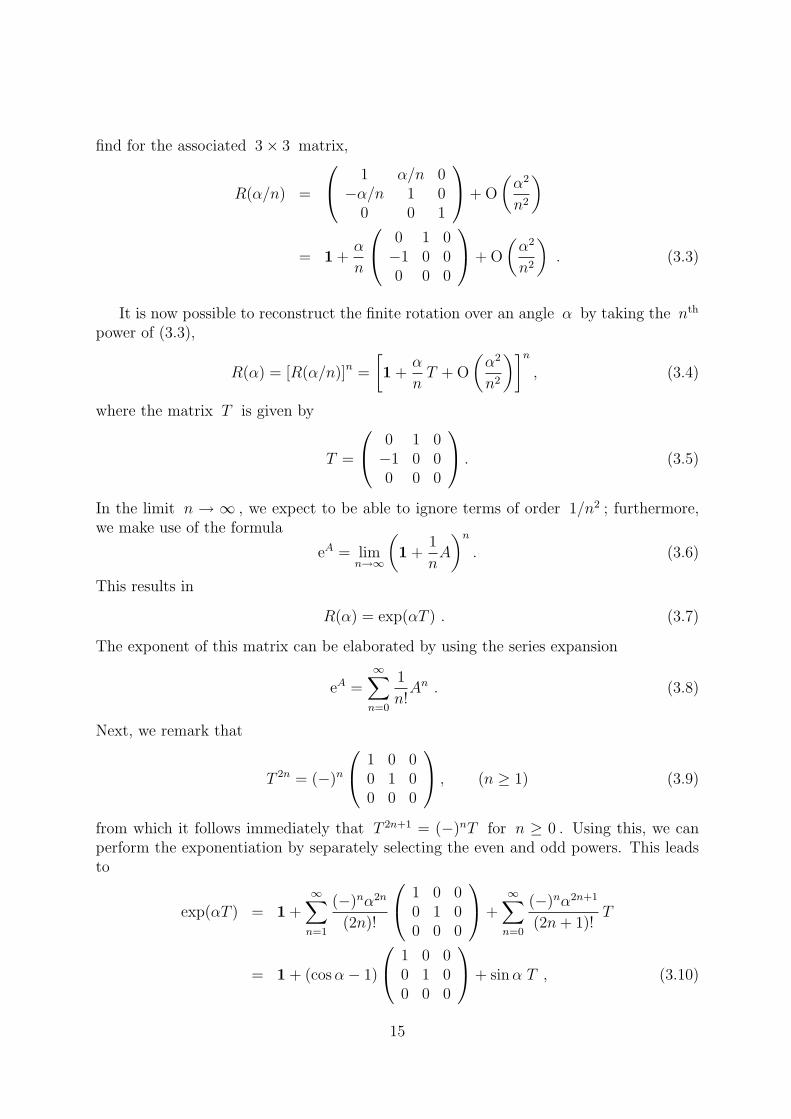
find for the associated 3× 3 matrix,
R(α/n) =
1 α/n 0−α/n 1 0
0 0 1
+ O
(α2
n2
)
= 1 +α
n
0 1 0−1 0 00 0 0
+ O
(α2
n2
). (3.3)
It is now possible to reconstruct the finite rotation over an angle α by taking the nth
power of (3.3),
R(α) = [R(α/n)]n =
[1 +
α
nT + O
(α2
n2
)]n
, (3.4)
where the matrix T is given by
T =
0 1 0−1 0 00 0 0
. (3.5)
In the limit n → ∞ , we expect to be able to ignore terms of order 1/n2 ; furthermore,we make use of the formula
eA = limn→∞
(1 +
1
nA
)n
. (3.6)
This results in
R(α) = exp(αT ) . (3.7)
The exponent of this matrix can be elaborated by using the series expansion
eA =∞∑
n=0
1
n!An . (3.8)
Next, we remark that
T 2n = (−)n
1 0 00 1 00 0 0
, (n ≥ 1) (3.9)
from which it follows immediately that T 2n+1 = (−)nT for n ≥ 0 . Using this, we canperform the exponentiation by separately selecting the even and odd powers. This leadsto
exp(αT ) = 1 +∞∑
n=1
(−)nα2n
(2n)!
1 0 00 1 00 0 0
+
∞∑n=0
(−)nα2n+1
(2n + 1)!T
= 1 + (cos α− 1)
1 0 00 1 00 0 0
+ sin α T , (3.10)
15
α
α
rr + r × α
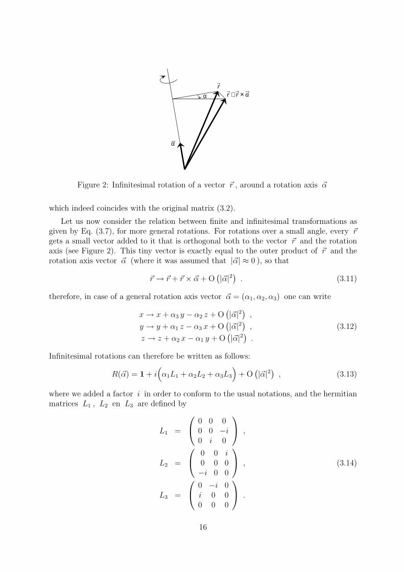
Figure 2: Infinitesimal rotation of a vector ~r , around a rotation axis ~α
which indeed coincides with the original matrix (3.2).
Let us now consider the relation between finite and infinitesimal transformations asgiven by Eq. (3.7), for more general rotations. For rotations over a small angle, every ~rgets a small vector added to it that is orthogonal both to the vector ~r and the rotationaxis (see Figure 2). This tiny vector is exactly equal to the outer product of ~r and therotation axis vector ~α (where it was assumed that |~α| ≈ 0 ), so that
~r → ~r + ~r × ~α + O(|~α|2) . (3.11)
therefore, in case of a general rotation axis vector ~α = (α1, α2, α3) one can write
x → x + α3 y − α2 z + O(|~α|2) ,
y → y + α1 z − α3 x + O(|~α|2) , (3.12)
z → z + α2 x− α1 y + O(|~α|2) .
Infinitesimal rotations can therefore be written as follows:
R(~α) = 1 + i(α1L1 + α2L2 + α3L3
)+ O
(|~α|2) , (3.13)
where we added a factor i in order to conform to the usual notations, and the hermitianmatrices L1 , L2 en L3 are defined by
L1 =
0 0 00 0 −i0 i 0
,
L2 =
0 0 i0 0 0−i 0 0
, (3.14)
L3 =
0 −i 0i 0 00 0 0
.
16
Above result can be compressed in one expression by using the completely skew-symmetricepsilon tensor,
(Li)jk = −iεijk . (3.15)
Indeed, we can easily check that
(L1)23 = − (L1)32 = −iε123 = −i ,
(L2)31 = − (L2)13 = −iε231 = −i , (3.16)
(L3)12 = − (L3)21 = −iε312 = −i .
Again, we can consider R(~α) as being formed out of n successive rotations withrotation axis ~α/n ,
R(~α) = [R(~α/n)]n
=
[1 +
1
n
(iα1L1 + iα2L2 + iα3L3
)+ O
( |~α|2n2
)]n
. (3.17)
Employing (3.4), we find then the following expression in the limit n →∞ ,
R(~α) = exp
(i∑
k
αkLk
). (3.18)
The correctness of Eq. (3.18) can be checked in a different way. First, we note thatthe following multiplication rule holds for rotations around one common axis of rotation,but with different rotation angles:
R(s~α) R(t~α) = R((s + t)~α) , (3.19)
where s and t are real numbers. The rotations R(s~α) with one common axis of rotationdefine a commuting subgroup of the complete rotation group. This is not difficult to see:The matrices R(s~α) (with a fixed vector ~α and a variable s ) define a group, where theresult of a multiplication does not depend on the order in the product,
R(s~α) R(t~α) = R(t~α) R(s~α) . (3.20)
This subgroup is the group SO(2) , the group of the two-dimensional rotations (the axisof rotation stays the same under these rotations, only the components of a vector that areorthogonal to the axis of rotation are rotated). Using Eq. (3.19), we can simply deducethe following differential equation for R(s~α) ,
d
dsR(s~α) = lim
∆→0
R((s + ∆)~α)−R(s~α)
∆
= lim∆→0
R(∆~α)− 1
∆R(s~α)
=
(i∑
k
αkLk
)R(s~α) , (3.21)
17
where first Eq. (3.19) was used, and subsequently (3.13). Now it is easy to verify that thesolution of this differential equation is exactly given by Eq. (3.18).
Yet an other way to ascertain that the matrices (3.18) represent rotations, is to provethat these matrices are orthogonal and have determinant equal to 1, which means thatthe following relations are fulfilled
R(~α) = [R(~α)]−1 = R(−~α) , det R(~α) = 1 , (3.22)
The proof follows from the following properties for a general matrix A (see also AppendixC),
(eA) = eeA , det
(eA
)= eTr A . (3.23)
From this, it follows that the matrices (3.18) obey Eqs. (3.22) provided that the matrixi∑
k αkLk be real and skew-symmetric. This indeed turns out to be the case; from thedefinitions (3.15) it follows that i
∑k αkLk in fact represents the most general real, and
skew-symmetric 3× 3 matrix.
The above question may actually be turned around: can all rotations be written in theform of Eq. (3.18)? The answer to this question is not quite so easy to give. In principle,the exponentiation in (3.18) can be performed explicitly via the power series expansion(3.8), and the result can be compared with the most general rotation matrix. It willturn out that the answer is affirmative: all rotations can indeed be written in the formof Eq. (3.18). This, however, is not the case for all groups. The so-called non-compactgroups contain elements that cannot be written as a product of a finite number of suchexponentials. These groups are called non-compact, because the volume of parameterspace is non-compact. The rotation group, where all possible group elements are definedin terms of the parameters αk that are restricted to the insides of a sphere with radiusπ , is a compact group. Within the frame of these lectures, non-compact groups willplay no role, but such groups are not unimportant in physics. The Lorentz group, forexample, which is the group consisting of all lorentz transformations, is an example of anon-compact group.
From the preceding discussion it will be clear that the matrices Lk , associated withthe infinitesimal transformations, will be important, and at least for the compact groups,they will completely determine the group elements, by means of the exponentiation (3.18).This is why these matrices are called the generators of the group. Although our discussionwas confined to the rotation group, the above can be applied to all Lie groups6: a groupwhose elements depend analytically on a finite number of parameters, in our case α1 , α2 ,and α3 . In the case that the group elements take the form of matrices, this means thatthe matrix elements must be differentiable functions of the parameters.7 The number oflinearly independent parameters defines the dimension of the Lie group, not to be confused
6Named after the Norwegian mathematician Sophus Lie, 1842-18997This is clearly the case for the rotation group. In the general case, the above requirement can
be somewhat weakened; for a general Lie group it suffices to require the elements as functions of theparameters to be twice differentiable.
18
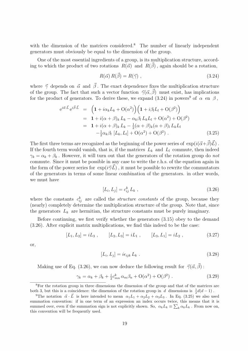
with the dimension of the matrices considered.8 The number of linearly independentgenerators must obviously be equal to the dimension of the group.
One of the most essential ingredients of a group, is its multiplication structure, accord-ing to which the product of two rotations R(~α) and R(~β) , again should be a rotation,
R(~α) R(~β) = R(~γ) , (3.24)
where ~γ depends on ~α and ~β . The exact dependence fixes the multiplication structureof the group. The fact that such a vector function ~γ(~α, ~β) must exist, has implicationsfor the product of generators. To derive these, we expand (3.24) in powers9 of α en β ,
ei~α·~L ei~β·~L =(1 + iαkLk + O(α2)
)(1 + iβlLl + O(β2)
)
= 1 + i(α + β)k Lk − αkβl LkLl + O(α2) + O(β2)
= 1 + i(α + β)k Lk − 12(α + β)k(α + β)l LkLl
−12αkβl [Lk, Ll] + O(α2) + O(β2) . (3.25)
The first three terms are recognized as the beginning of the power series of exp(i(~α+~β)·~L) .If the fourth term would vanish, that is, if the matrices Lk and Ll commute, then indeedγk = αk + βk . However, it will turn out that the generators of the rotation group do notcommute. Since it must be possible in any case to write the r.h.s. of the equation again inthe form of the power series for exp(i~γ·~L) , it must be possible to rewrite the commutatorsof the generators in terms of some linear combination of the generators. in other words,we must have
[Li, Lj] = ckij Lk , (3.26)
where the constants ckij are called the structure constants of the group, because they
(nearly) completely determine the multiplication structure of the group. Note that, sincethe generators Lk are hermitian, the structure constants must be purely imaginary.
Before continuing, we first verify whether the generators (3.15) obey to the demand(3.26). After explicit matrix multiplications, we find this indeed to be the case:
[L1, L2] = iL3 , [L2, L3] = iL1 , [L3, L1] = iL2 , (3.27)
or,
[Li, Lj] = iεijk Lk . (3.28)
Making use of Eq. (3.26), we can now deduce the following result for ~γ(~α, ~β) :
γk = αk + βk + i2ckmn αmβn + O(α2) + O(β2) . (3.29)
8For the rotation group in three dimensions the dimension of the group and that of the matrices areboth 3, but this is a coincidence: the dimension of the rotation group in d dimensions is 1
2d(d− 1) .9The notation ~α · ~L is here intended to mean α1L1 + α2L2 + α3L3 . In Eq. (3.25) we also used
summation convention: if in one term of an expression an index occurs twice, this means that it issummed over, even if the summation sign is not explicitly shown. So, αkLk ≡
∑k αkLk . From now on,
this convention will be frequently used.
19
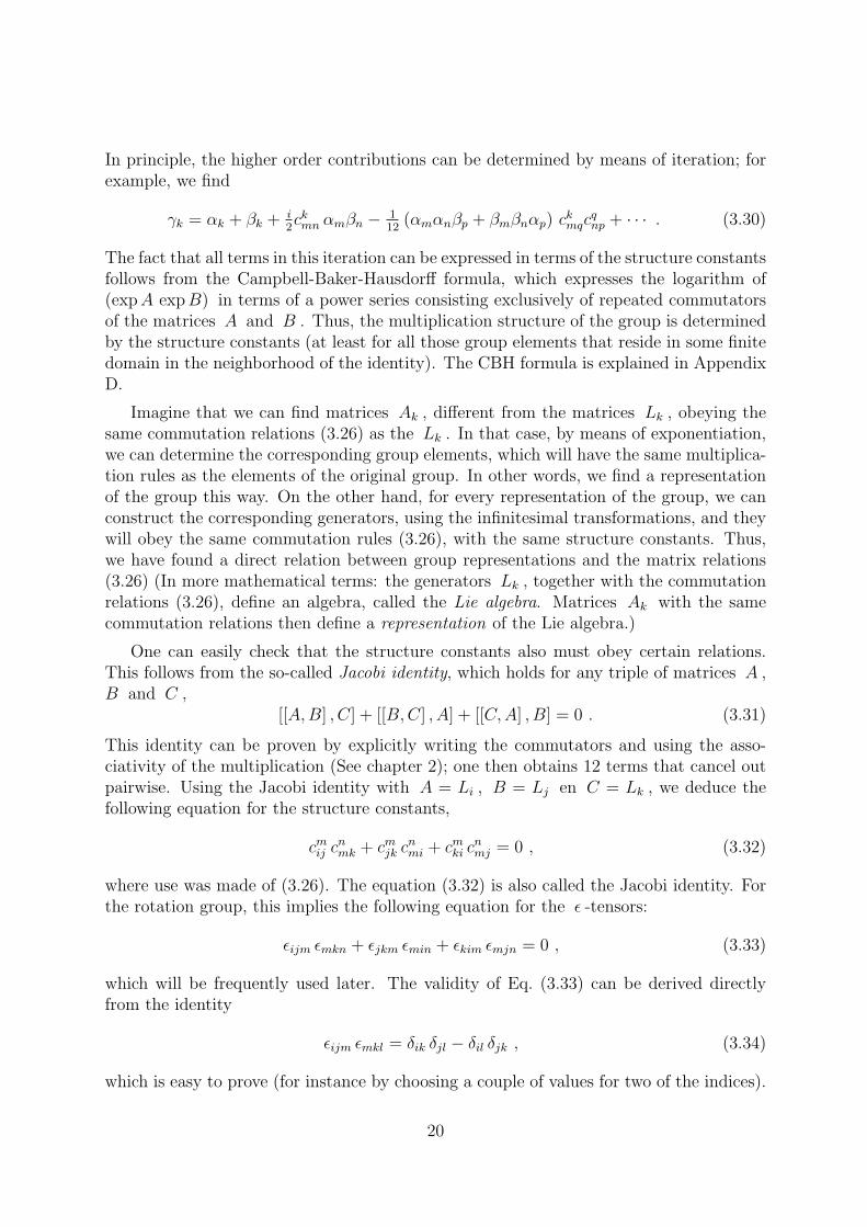
In principle, the higher order contributions can be determined by means of iteration; forexample, we find
γk = αk + βk + i2ckmn αmβn − 1
12(αmαnβp + βmβnαp) ck
mqcqnp + · · · . (3.30)
The fact that all terms in this iteration can be expressed in terms of the structure constantsfollows from the Campbell-Baker-Hausdorff formula, which expresses the logarithm of(exp A exp B) in terms of a power series consisting exclusively of repeated commutatorsof the matrices A and B . Thus, the multiplication structure of the group is determinedby the structure constants (at least for all those group elements that reside in some finitedomain in the neighborhood of the identity). The CBH formula is explained in AppendixD.
Imagine that we can find matrices Ak , different from the matrices Lk , obeying thesame commutation relations (3.26) as the Lk . In that case, by means of exponentiation,we can determine the corresponding group elements, which will have the same multiplica-tion rules as the elements of the original group. In other words, we find a representationof the group this way. On the other hand, for every representation of the group, we canconstruct the corresponding generators, using the infinitesimal transformations, and theywill obey the same commutation rules (3.26), with the same structure constants. Thus,we have found a direct relation between group representations and the matrix relations(3.26) (In more mathematical terms: the generators Lk , together with the commutationrelations (3.26), define an algebra, called the Lie algebra. Matrices Ak with the samecommutation relations then define a representation of the Lie algebra.)
One can easily check that the structure constants also must obey certain relations.This follows from the so-called Jacobi identity, which holds for any triple of matrices A ,B and C ,
[[A,B] , C] + [[B, C] , A] + [[C, A] , B] = 0 . (3.31)
This identity can be proven by explicitly writing the commutators and using the asso-ciativity of the multiplication (See chapter 2); one then obtains 12 terms that cancel outpairwise. Using the Jacobi identity with A = Li , B = Lj en C = Lk , we deduce thefollowing equation for the structure constants,
cmij cn
mk + cmjk cn
mi + cmki c
nmj = 0 , (3.32)
where use was made of (3.26). The equation (3.32) is also called the Jacobi identity. Forthe rotation group, this implies the following equation for the ε -tensors:
εijm εmkn + εjkm εmin + εkim εmjn = 0 , (3.33)
which will be frequently used later. The validity of Eq. (3.33) can be derived directlyfrom the identity
εijm εmkl = δik δjl − δil δjk , (3.34)
which is easy to prove (for instance by choosing a couple of values for two of the indices).
20
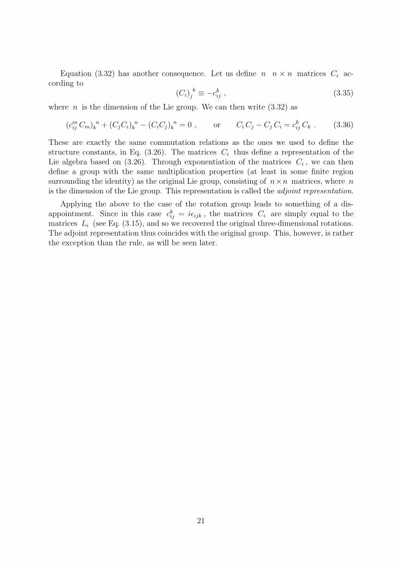
Equation (3.32) has another consequence. Let us define n n × n matrices Ci ac-cording to
(Ci)k
j ≡ −ckij , (3.35)
where n is the dimension of the Lie group. We can then write (3.32) as
(cmij Cm) n
k + (CjCi)n
k − (CiCj)n
k = 0 , or Ci Cj − Cj Ci = ckij Ck . (3.36)
These are exactly the same commutation relations as the ones we used to define thestructure constants, in Eq. (3.26). The matrices Ci thus define a representation of theLie algebra based on (3.26). Through exponentiation of the matrices Ci , we can thendefine a group with the same multiplication properties (at least in some finite regionsurrounding the identity) as the original Lie group, consisting of n×n matrices, where nis the dimension of the Lie group. This representation is called the adjoint representation.
Applying the above to the case of the rotation group leads to something of a dis-appointment. Since in this case ck
ij = iεijk , the matrices Ci are simply equal to thematrices Li (see Eq. (3.15), and so we recovered the original three-dimensional rotations.The adjoint representation thus coincides with the original group. This, however, is ratherthe exception than the rule, as will be seen later.
21
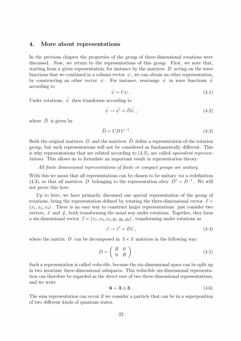
4. More about representations
In the previous chapter the properties of the group of three-dimensional rotations werediscussed. Now, we return to the representations of this group. First, we note that,starting from a given representation, for instance by the matrices D acting on the wavefunctions that we combined in a column vector ψ , we can obtain an other representation,by constructing an other vector ψ . For instance, rearrange ψ in wave functions ψaccording to
ψ = Uψ . (4.1)
Under rotations, ψ then transforms according to
ψ → ψ′ = Dψ , (4.2)
where D is given by
D = UD U−1 . (4.3)
Both the original matrices D and the matrices D define a representation of the rotationgroup, but such representations will not be considered as fundamentally different. Thisis why representations that are related according to (4.3), are called equivalent represen-tations. This allows us to formulate an important result in representation theory:
All finite dimensional representations of finite or compact groups are unitary.
With this we mean that all representations can be chosen to be unitary via a redefinition(4.3), so that all matrices D belonging to the representation obey D† = D−1 . We willnot prove this here.
Up to here, we have primarily discussed one special representation of the group ofrotations, being the representation defined by rotating the three-dimensional vector ~x =(x1, x2, x3) . There is an easy way to construct larger representations: just consider twovectors, ~x and ~y , both transforming the usual way under rotations. Together, they forma six-dimensional vector ~z = (x1, x2, x3, y1, y2, y3) , transforming under rotations as
~z → ~z ′ = D~z , (4.4)
where the matrix D can be decomposed in 3× 3 matrices in the following way:
D =
(R 00 R
). (4.5)
Such a representation is called reducible, because the six-dimensional space can be split upin two invariant three-dimensional subspaces. This reducible six-dimensional representa-tion can therefore be regarded as the direct sum of two three-dimensional representations,and we write
6 = 3⊕ 3 . (4.6)
The sum representation can occur if we consider a particle that can be in a superpositionof two different kinds of quantum states.
22
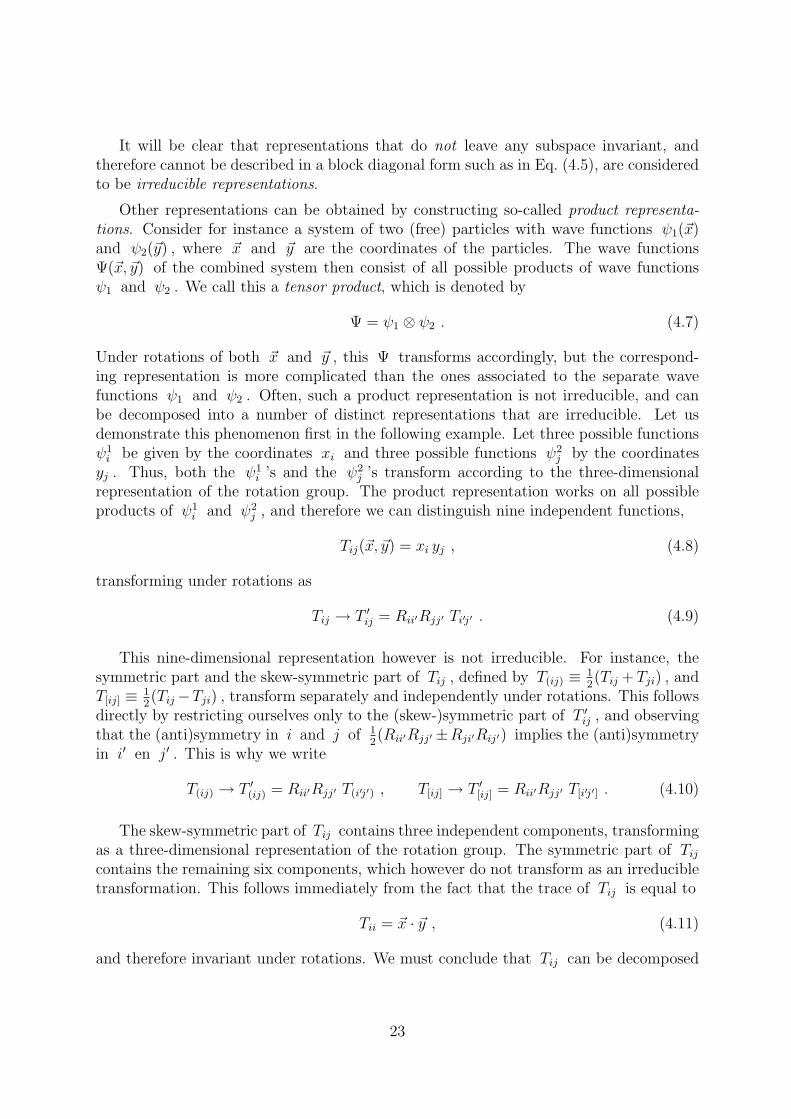
It will be clear that representations that do not leave any subspace invariant, andtherefore cannot be described in a block diagonal form such as in Eq. (4.5), are consideredto be irreducible representations.
Other representations can be obtained by constructing so-called product representa-tions. Consider for instance a system of two (free) particles with wave functions ψ1(~x)and ψ2(~y) , where ~x and ~y are the coordinates of the particles. The wave functionsΨ(~x, ~y) of the combined system then consist of all possible products of wave functionsψ1 and ψ2 . We call this a tensor product, which is denoted by
Ψ = ψ1 ⊗ ψ2 . (4.7)
Under rotations of both ~x and ~y , this Ψ transforms accordingly, but the correspond-ing representation is more complicated than the ones associated to the separate wavefunctions ψ1 and ψ2 . Often, such a product representation is not irreducible, and canbe decomposed into a number of distinct representations that are irreducible. Let usdemonstrate this phenomenon first in the following example. Let three possible functionsψ1
i be given by the coordinates xi and three possible functions ψ2j by the coordinates
yj . Thus, both the ψ1i ’s and the ψ2
j ’s transform according to the three-dimensionalrepresentation of the rotation group. The product representation works on all possibleproducts of ψ1
i and ψ2j , and therefore we can distinguish nine independent functions,
Tij(~x, ~y) = xi yj , (4.8)
transforming under rotations as
Tij → T ′ij = Rii′Rjj′ Ti′j′ . (4.9)
This nine-dimensional representation however is not irreducible. For instance, thesymmetric part and the skew-symmetric part of Tij , defined by T(ij) ≡ 1
2(Tij + Tji) , and
T[ij] ≡ 12(Tij−Tji) , transform separately and independently under rotations. This follows
directly by restricting ourselves only to the (skew-)symmetric part of T ′ij , and observing
that the (anti)symmetry in i and j of 12(Rii′Rjj′±Rji′Rij′) implies the (anti)symmetry
in i′ en j′ . This is why we write
T(ij) → T ′(ij) = Rii′Rjj′ T(i′j′) , T[ij] → T ′
[ij] = Rii′Rjj′ T[i′j′] . (4.10)
The skew-symmetric part of Tij contains three independent components, transformingas a three-dimensional representation of the rotation group. The symmetric part of Tij
contains the remaining six components, which however do not transform as an irreducibletransformation. This follows immediately from the fact that the trace of Tij is equal to
Tii = ~x · ~y , (4.11)
and therefore invariant under rotations. We must conclude that Tij can be decomposed
23
in three independent tensors10,
Tij →
T = ~x · ~yTi = εijkxjyk
Sij = xiyj + xjyi − 23δij(~x · ~y)
. (4.12)
Note that we used the epsilon symbol to describe the skew-symmetric part of Tij again as
a three-dimensional vector ~T (it is nothing but the outer product ~x× ~y ). Furthermore,we made the symmetric part Sij traceless by adding an extra term proportional to δij .The consequence of this is that Sij consists of only five independent components. Underrotations, the terms listed above transform into expressions of the same type; the fiveindependent components of Sij transform into one another.11 In short, the product oftwo three-dimensional representations can be written as
3⊗ 3 = 1⊕ 3⊕ 5 , (4.13)
where the representations are characterized by their dimensions (temporarily ignoringthe fact that inequivalent irreducible representations might exist with equal numbers ofdimensions; they don’t here, as we will see later).
The procedure followed in this example, rests on two features; first, we use that thesymmetry properties of tensors do not change under the transformations, and secondlywe make use of the existence of two invariant tensors, to wit:
Tij = δij , Tijk = εijk . (4.14)
An invariant tensor is a tensor that does not change at all under the group transformations,as they act according to the index structure of the tensor, so that
Tijk··· → T ′ijk··· = Rii′Rjj′Rkk′ · · · Ti′j′k′··· = Tijk··· . (4.15)
Indeed, both tensors δij and εijk obey (4.15), since the equation
Rii′Rjj′ δi′j′ = δij (4.16)
is fulfilled because the Rij are orthogonal matrices, and
Rii′Rjj′Rkk′ εi′j′k′ = det R εijk = εijk (4.17)
10In the second equation, again summation convention is used, see an earlier footnote.11For each of these representations, we can indicate the matrices D(R) that are defined in chapter 2.
For the first representation, we have that D(R) = 1 . In the second representation, we have 3 × 3matrices D(R) equal to the matrix R . For the third representation, we have 5 × 5 matrices D(R) .The indices of this correspond to the symmetric, traceless index pairs ij . The matrices D(R) can bewritten as
D(R)(ij) (kl) =12
(Rik Rjl + Ril Rjk)− 13δij δkl .
24
holds because the rotation matrices Rij have det R = 1 . For every given tensor Tijk··· wecan contract the indices using invariant tensors. It is then evident that tensors contractedthat way span invariant subspaces, in other words, under rotations they will transform intotensors that are formed the same way. For example, let Tijk··· be a tensor transforminglike
Tijk··· → T ′ijk··· = Rii′Rjj′Rkk′ · · · Ti′j′k′··· . (4.18)
Now, form the tensorTklm··· ≡ δij Tijklm··· (4.19)
which has two indices less. By using Eq, (4.16), it is now easy to check that T transformsas
Tklm··· → T ′klm··· = Rkk′Rll′Rmm′ · · · Tk′l′m′··· , (4.20)
and, in a similar way, we can verify that contractions with one or more δ and ε tensors,produce tensors that span invariant subspaces. Using the example discussed earlier, wecan write the expansion as
Tij =1
2εijk (εklm Tlm) +
1
2
(Tij + Tji − 2
3δijTkk
)+
1
3δij Tkk , (4.21)
where the first term can also be written as 12(Tij − Tji) , by using the identity (3.34),
εijk εklm = δilδjm − δimδjl , (4.22)
and the second term in (4.21) is constructed in such a way that it is traceless:
δij
(Tij + Tji − 2
3δijTkk
)= 0 . (4.23)
25
5. Ladder operators
Let us consider a representation of the rotation group, generated by hermitian matricesI1 , I2 and I3 , which obey the same commutation rules as L1 , L2 and L3 , given inEq. (3.15),
[I1, I2] = iI3 , [I2, I3] = iI1 , [I3, I1] = iI2 , (5.1)
or in shorthand:
[Ii, Ij] = iεijk Ik . (5.2)
We demand the matrices exp(iαkIk) to be unitary; therefore, the Ii are hermitian:I†i = Ii . Starting from this information, we now wish to determine all sets of irreduciblematrices Ii with these properties. This is the way to determine all (finite-dimensional,unitary) representations of the group of rotations in three dimensions.
To this end, first define the linear combinations
I± = I1 ± iI2 , (5.3)
so that (I±)† = I∓ , and
[I3, I±] = [I3, I1]± i[I3, I2] = iI2 ± I1 = ±I± . (5.4)
So we have for any state | ψ〉 ,
I3
(I+ | ψ〉
)= I+(I3 + 1) | ψ〉 . (5.5)
A Casimir operator is a combination of operators for a representation constructed in sucha way that it commutes with all generators. Schur’s lemma states the following: if andonly if the representation is irreducible, every Casimir operator will be a multiple of theunit matrix.
In the case of the three-dimensional rotations, we have such a Casimir operator:
~I 2 ≡ I21 + I2
2 + I23 . (5.6)
We derive from Eq. (5.1):
[~I 2, I1] = [~I 2, I2] = [~I 2, I3] = 0 . (5.7)
Since ~I 2 en I3 are two commuting matrices, we can find a basis of states such that ~I 2
and I3 both at the same time take a diagonal form, with real eigenvalues. Furthermore,the eigenvalues of ~I 2 must be positive (or zero), because we have
〈ψ | ~I 2 | ψ〉 =∣∣∣I1 | ψ〉
∣∣∣2
+∣∣∣I2 | ψ〉
∣∣∣2
+∣∣∣I3 | ψ〉
∣∣∣2
≥ 0 . (5.8)
26
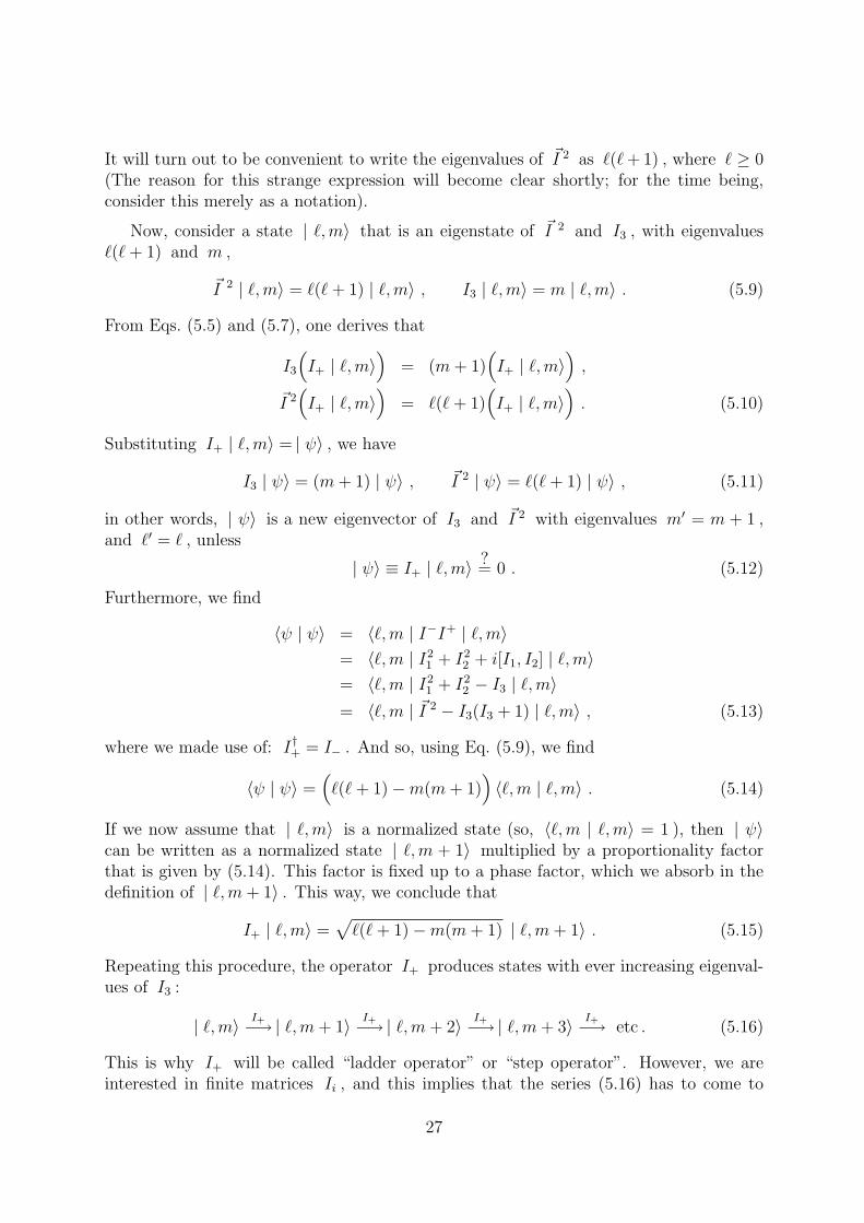
It will turn out to be convenient to write the eigenvalues of ~I 2 as `(` + 1) , where ` ≥ 0(The reason for this strange expression will become clear shortly; for the time being,consider this merely as a notation).
Now, consider a state | `, m〉 that is an eigenstate of ~I 2 and I3 , with eigenvalues`(` + 1) and m ,
~I 2 | `,m〉 = `(` + 1) | `,m〉 , I3 | `,m〉 = m | `,m〉 . (5.9)
From Eqs. (5.5) and (5.7), one derives that
I3
(I+ | `,m〉
)= (m + 1)
(I+ | `,m〉
),
~I 2(I+ | `,m〉
)= `(` + 1)
(I+ | `,m〉
). (5.10)
Substituting I+ | `, m〉 = | ψ〉 , we have
I3 | ψ〉 = (m + 1) | ψ〉 , ~I 2 | ψ〉 = `(` + 1) | ψ〉 , (5.11)
in other words, | ψ〉 is a new eigenvector of I3 and ~I 2 with eigenvalues m′ = m + 1 ,and `′ = ` , unless
| ψ〉 ≡ I+ | `,m〉 ?= 0 . (5.12)
Furthermore, we find
〈ψ | ψ〉 = 〈`,m | I−I+ | `,m〉= 〈`,m | I2
1 + I22 + i[I1, I2] | `,m〉
= 〈`,m | I21 + I2
2 − I3 | `, m〉= 〈`,m | ~I 2 − I3(I3 + 1) | `,m〉 , (5.13)
where we made use of: I†+ = I− . And so, using Eq. (5.9), we find
〈ψ | ψ〉 =(`(` + 1)−m(m + 1)
)〈`,m | `,m〉 . (5.14)
If we now assume that | `,m〉 is a normalized state (so, 〈`,m | `,m〉 = 1 ), then | ψ〉can be written as a normalized state | `, m + 1〉 multiplied by a proportionality factorthat is given by (5.14). This factor is fixed up to a phase factor, which we absorb in thedefinition of | `,m + 1〉 . This way, we conclude that
I+ | `,m〉 =√
`(` + 1)−m(m + 1) | `,m + 1〉 . (5.15)
Repeating this procedure, the operator I+ produces states with ever increasing eigenval-ues of I3 :
| `,m〉 I+−→| `,m + 1〉 I+−→| `,m + 2〉 I+−→| `,m + 3〉 I+−→ etc . (5.16)
This is why I+ will be called “ladder operator” or “step operator”. However, we areinterested in finite matrices Ii , and this implies that the series (5.16) has to come to
27
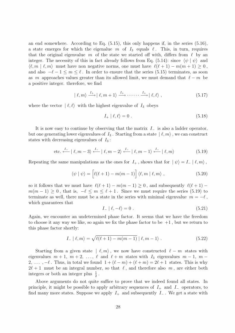
an end somewhere. According to Eq. (5.15), this only happens if, in the series (5.16),a state emerges for which the eigenalue m of I3 equals ` . This, in turn, requiresthat the original eigenvalue m of the state we started off with, differs from ` by aninteger. The necessity of this in fact already follows from Eq. (5.14): since 〈ψ | ψ〉 and〈`,m | `, m〉 must have non negative norms, one must have `(` + 1) − m(m + 1) ≥ 0 ,and also −` − 1 ≤ m ≤ ` . In order to ensure that the series (5.15) terminates, as soonas m approaches values greater than its allowed limit, we must demand that `−m bea positive integer. therefore, we find
| `,m〉 I+−→| `,m + 1〉 I+−→ · · · · · · I+−→| `, `〉 , (5.17)
where the vector | `, `〉 with the highest eigenvalue of I3 obeys
I+ | `, `〉 = 0 . (5.18)
It is now easy to continue by observing that the matrix I− is also a ladder operator,but one generating lower eigenvalues of I3 . Starting from a state | `,m〉 , we can constructstates with decreasing eigenvalues of I3 :
etc.I−←−| `,m− 3〉 I−←−| `,m− 2〉 I−←−| `,m− 1〉 I−←−| `,m〉 (5.19)
Repeating the same manipulations as the ones for I+ , shows that for | ψ〉 = I− | `,m〉 ,
〈ψ | ψ〉 =[`(` + 1)−m(m− 1)
]〈`,m | `,m〉 , (5.20)
so it follows that we must have `(` + 1) −m(m − 1) ≥ 0 , and subsequently `(` + 1) −m(m − 1) ≥ 0 , that is, −` ≤ m ≤ ` + 1 . Since we must require the series (5.19) toterminate as well, there must be a state in the series with minimal eigenvalue m = −` ,which guarantees that
I− | `,−`〉 = 0 . (5.21)
Again, we encounter an undetermined phase factor. It seems that we have the freedomto choose it any way we like, so again we fix the phase factor to be +1 , but we return tothis phase factor shortly:
I− | `,m〉 =√
`(` + 1)−m(m− 1) | `,m− 1〉 . (5.22)
Starting from a given state | `,m〉 , we now have constructed ` − m states witheigenvalues m + 1, m + 2, . . . , ` and ` + m states with I3 eigenvalues m − 1, m −2, . . . ,−` . Thus, in total we found 1 + (`−m) + (` + m) = 2` + 1 states. This is why2` + 1 must be an integral number, so that ` , and therefore also m , are either bothintegers or both an integer plus 1
2.
Above arguments do not quite suffice to prove that we indeed found all states. Inprinciple, it might be possible to apply arbitrary sequences of I+ and I− operators, tofind many more states. Suppose we apply I+ and subsequently I− . We get a state with
28

the same values of both ` and m as before. But is this the same state? Indeed, theanswer is yes — and also the phase is +1 ! Note that
I− I+ = I21 + I2
2 + i(I1 I2 − I2 I1) = (~I)2 − I23 − I3 =
(`(` + 1)−m(m + 1)
)1 . (5.23)
This ensures that, if we apply (5.15) and (5.22) in succession, we get back exactly thesame state as the one we started off with (correctly normalized, and with a phase factor+1 ).
By way of exercise, we verify that the operators I+, I− and I3 exclusively act on thissingle series of states | `,m〉 as prescribed by Eqs. (5.9), (5.15), and (5.22). Checking thecommutation rules,
[I3, I±, ] = ±I± , [I+, I−] = 2I3 , (5.24)
we indeed find
(I3I± − I±I3) | `,m〉 = (m± 1)√
`(` + 1)−m(m± 1) | `,m± 1〉−m
√`(` + 1)−m(m± 1) | `,m± 1〉
= ±√
`(` + 1)−m(m± 1) | `,m± 1〉= ±I± | `,m〉 , (5.25)
(I+I− − I−I+) | `,m〉 =√
`(` + 1)− (m− 1)m√
`(` + 1)− (m− 1)m | `,m〉−
√`(` + 1)− (m + 1)m
√`(` + 1)− (m + 1)m | `, m〉
= 2m | `,m〉= 2I3 | `,m〉 . (5.26)
Summarizing, we found that an irreducible representation of I1 , I2 , I3 can be char-acterized by a number ` , and it acts on a space spanned by 2` + 1 states | `,m〉 forwhich
~I 2 | `,m〉 = `(` + 1) | `,m〉 ,
I3 | `,m〉 = m | `,m〉 ,
I± | `,m〉 =√
`(` + 1)−m(m± 1) | `,m± 1〉 , (5.27)
with m = −`, −` + 1, ,−` + 2, · · · , `− 2, `− 1, ` . Either both ` and m are integers,or they are both integers plus 1
2. Of course, we always have I1 = 1
2(I+ + I−) and
I2 = 12i
(I+ − I−) .
We now provide some examples, being the representations for ` = 0, 12, 1 , and 3
2:
• For ` = 0 , we find the trivial representation. There is only one state, |0, 0〉 , andIi|0, 0〉 = 0 for i = 1, 2, 3.
29
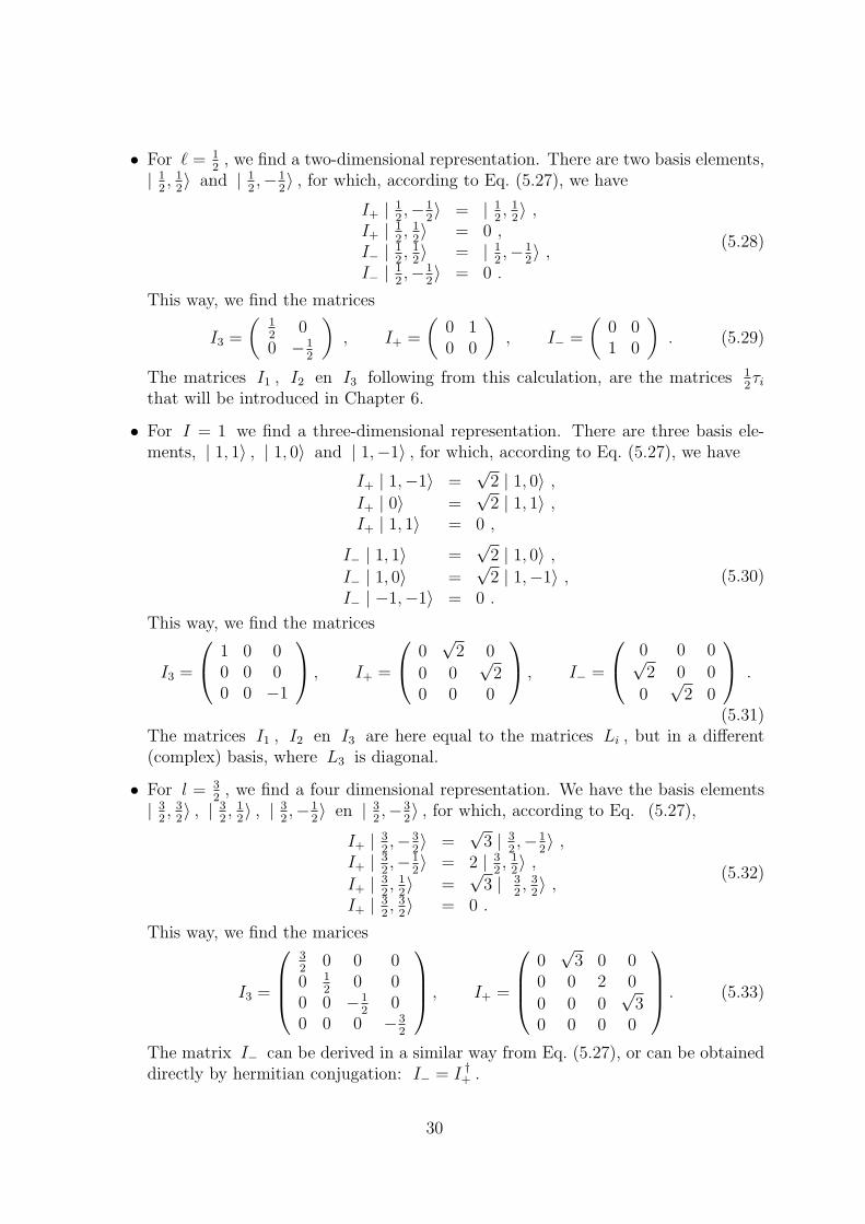
• For ` = 12
, we find a two-dimensional representation. There are two basis elements,| 1
2, 1
2〉 and | 1
2,−1
2〉 , for which, according to Eq. (5.27), we have
I+ | 12,−1
2〉 = | 1
2, 1
2〉 ,
I+ | 12, 1
2〉 = 0 ,
I− | 12, 1
2〉 = | 1
2,−1
2〉 ,
I− | 12,−1
2〉 = 0 .
(5.28)
This way, we find the matrices
I3 =
(12
00 −1
2
), I+ =
(0 10 0
), I− =
(0 01 0
). (5.29)
The matrices I1 , I2 en I3 following from this calculation, are the matrices 12τi
that will be introduced in Chapter 6.
• For I = 1 we find a three-dimensional representation. There are three basis ele-ments, | 1, 1〉 , | 1, 0〉 and | 1,−1〉 , for which, according to Eq. (5.27), we have
I+ | 1,−1〉 =√
2 | 1, 0〉 ,
I+ | 0〉 =√
2 | 1, 1〉 ,I+ | 1, 1〉 = 0 ,
I− | 1, 1〉 =√
2 | 1, 0〉 ,
I− | 1, 0〉 =√
2 | 1,−1〉 ,I− | −1,−1〉 = 0 .
(5.30)
This way, we find the matrices
I3 =
1 0 00 0 00 0 −1
, I+ =
0√
2 0
0 0√
20 0 0
, I− =
0 0 0√2 0 0
0√
2 0
.
(5.31)The matrices I1 , I2 en I3 are here equal to the matrices Li , but in a different(complex) basis, where L3 is diagonal.
• For l = 32
, we find a four dimensional representation. We have the basis elements| 3
2, 3
2〉 , | 3
2, 1
2〉 , | 3
2,−1
2〉 en | 3
2,−3
2〉 , for which, according to Eq. (5.27),
I+ | 32,−3
2〉 =
√3 | 3
2,−1
2〉 ,
I+ | 32,−1
2〉 = 2 | 3
2, 1
2〉 ,
I+ | 32, 1
2〉 =
√3 | 3
2, 3
2〉 ,
I+ | 32, 3
2〉 = 0 .
(5.32)
This way, we find the marices
I3 =
32
0 0 00 1
20 0
0 0 −12
00 0 0 −3
2
, I+ =
0√
3 0 00 0 2 0
0 0 0√
30 0 0 0
. (5.33)
The matrix I− can be derived in a similar way from Eq. (5.27), or can be obtaineddirectly by hermitian conjugation: I− = I †+ .
30
6. The group SU (2)
In Chapter 4, we only saw irreducible representations of the three-dimensional rotationgroup that were all odd dimensional. Chapter 5, however, showed the complete set ofall irreducible representations of this group, and as many of them are even as there areodd ones. More understanding of the even-dimensional representations is needed. Tothis end, we subject the simplest example of these, the one with ` = 1
2, to a closer
inspection. Clearly, we have vectors forming a two-dimensional space, which will becalled spinors. Every rotation in a three-dimensional space must be associated to aunitary transformation in this spinor space. If R = exp(i
∑k αkLk) , then the associated
transformation X is written as X = exp(i∑
k αkIk) , where the generators Ik followfrom Eq. (5.29):
I1 =I+ + I−
2= 1
2τ1 , I2 =
I+ − I−2i
= 12τ2 , I3 = 1
2τ3 . (6.1)
Here, we have introduced the following three fundamental 2× 2 matrices: 12
τ1 =
(0 11 0
), τ2 =
(0 −ii 0
), τ3 =
(1 00 −1
). (6.2)
These τ -matrices obey the following product rules:
τi τj = δij1 + iεijk τk , (6.3)
as can easily be established. Since [τi, τj] = τi τj − τj τi , we find that the generators Ik
indeed obey the correct commutation rules:[τi
2,τj
2
]= iεijk
τk
2. (6.4)
The three τ matrices are hermitian and traceless :
τi = τ †i ; Tr (τi) = 0 . (6.5)
For rotations over tiny angles, |~α| ¿ 1 , the associated matrix X(~α) takes the fol-lowing form:
X(~α) = 1 + iB + O(B2) ; B = αiτi
2. (6.6)
One readily verifies that X(~α) is unitary and that its determinant equals 1:
(1 + iB + O(B2)
)†=
(1 + iB + O(B2)
)−1= 1− iB + O(B2) ;
det(1 + iB + O(B2)
)= 1 + i Tr B + O(B2) = 1 , (6.7)
sinceB† = B , Tr B = 0 . (6.8)
12Also called Pauli matrices, and often indicated as σi .
31
The finite transformation X(~α) is found by exponentiation of (6.6), exactly in accor-dance with the limiting procedure displayed in Chapter 3:
X(~α) = limn→∞
1 + i
αi
n
τi
2
n
= exp(iαi
τi
2
). (6.9)
The matrices 12τi are therefore the generators of the rotations for the ` = 1
2representa-
tion. They do require the coefficients 12
in order to obey exactly the same commutationrules as the generators Li of the rotation group in three dimensions, see Eq. (6.4).
By making use of the product property of the τ -matrices, we can calculate the expo-nential expression for X(~α) . This is done as follows:
X(~α) = eiαiτi/2
=∞∑
n=0
1
n!
(iαjτj
2
)n
=∞∑
n=0
1
(2n)!
(iαjτj
2
)2n
+∞∑
n=0
1
(2n + 1)!
(iαjτj
2
)2n+1
, (6.10)
where, in the last line, we do the summation over the even and the odd powers of (iαjτj)separately. Now we note that
(iαjτj)2 = −αjαk τj τk = −α2 1, (6.11)
where use was made of Eq. (6.3), and α is defined as
α =√
α 21 + α 2
2 + α 23 . (6.12)
From Eq. (6.11) it immediately follows that
(iαjτj)2n = (−)n α2n 1, (iαjτj)
2n+1 = (−)n α2n (iαjτj) , (6.13)
so that we can write Eq. (6.10) as
X(~α) =
∞∑n=0
(−)n
(2n)!
(α
2
)2n
1 +
∞∑n=0
(−)n
(2n + 1)!
(α
2
)2n+1 (
iαjτj
α
)
= cosα
21 + i sin
α
2
αjτj
α. (6.14)
It so happens that every 2× 2 matrix can be decomposed in the unit matrix 1 andτi :
X = c0 1 + ici τi. (6.15)
If we furthermore use the product rule (6.3) and Eq. (6.5), and also
Tr (1) = 2 , (6.16)
32
the coefficients c0 and ci can be determined for every 2× 2 matrix X :
c0 = 12Tr (X) ; ci = 1
2Tr (X τi) . (6.17)
In our case, we read off the coefficients c0 and ci directly from Eq. (6.14):
c0 = cosα
2, ci =
αi
αsin
α
2. (6.18)
It is clear that all these coefficients are real. Furthermore, we simply establish:
c20 + c2
i = 1. (6.19)
The expression (6.15) for X(~α) can now also be written in terms of two complexparameters a en b ,
X =
(a b−b∗ a∗
), (6.20)
with |a|2 + |b|2 = 1 . Matrices of the form (6.20) with generic a and b obeying|a|2 + |b|2 = 1 form the elements of the group SU(2) , the group of unitary 2 × 2matrices with determinant 1, because 13 they obey:
X† = X−1, det X = 1 . (6.21)
It should be clear that these matrices form a group: if X1 en X2 both obey (6.21)and (6.20), then also X3 = X1X2 and so this matrix also is an element of the group.Furthermore, the unit matrix and the inverse matrix obey (6.20) en (6.21), so they alsoare in the group, while associativity for the multiplication is evident as well.
In chapter 3 we established that the rotations can be parameterized by vectors ~α thatlie in a sphere with radius α = π . The direction of ~α coincides with the axis of rotation,and its length α equals the angle of rotation. Since rotations over +π and −π radiansare equal, we established that
R(~α) = R(−~α) , if α = π . (6.22)
As we see in Eq. (6.14), the elements of SU(2) can be parameterized by the same vectors~α . However, to parameterize all elements X(~α) , the radius of the sphere must be taken tobe twice as large, that is, equal to 2π . Again consider two vectors in opposite directions,~α and ~α ′ , in this sphere, such that the lengths α+α ′ = 2π , so that they yield the samerotation,
R(~α ′) = R(~α) , (6.23)
just because they rotate over the same axis with a difference of 2π in the angles. Thetwo associated SU(2) elements, X(~α ′) and X(~α) , however, are opposite to each other:
X(~α ′) = −X(~α) . (6.24)
13Similarly, the complex numbers with norm 1 form the group U(1) , which simply consists of all phasefactors exp iα .
33
This follows from Eqs. (6.14), (6.18) and the fact that cos α′2
= − cos α2
en sin α′2
= sin α2
.
The above implies that, strictly speaking, the elements of SU(2) are not a represen-tation of the three-dimensional rotation group, but a projective representation. After all,in the product of the rotations
R(~α) R(~β) = R(~γ), (6.25)
with α , β , we would also have γ ≤ π , but the product of the associated SU(2) matrices,
X(~α) X(~β) = ±X(~γ) , (6.26)
the value of γ depends on α and β but its length can be either larger or smaller than π ,so we may or may not have to include a minus sign in the equation14 if we wish to restrictourselves to vectors shorter than π . The group SU(2) does have the same structureconstants, and thus the same group product structure, as the rotation group, but thelatter only holds true in a small domain surrounding the unit element, and not exactlyfor the entire group.
A spinor ϕα transforms as follows:
ϕα → ϕα′ = Xαβ ϕβ . (6.27)
The complex conjugated vectors then transform as
ϕ∗α → ϕ∗′α = (Xαβ)∗ ϕ∗β = (X†)β
α ϕ∗β . (6.28)
Here, we introduced an important new notation: the indices are sometimes in a raisedposition (superscripts), and sometimes lowered (subscripts). This is done to indicate thatspinors with superscripts, such as in (6.27), transform differently under a rotation thanspinors with subscripts, such as (6.28). Upon complex conjugation, a superscript indexbecomes a subscript, and vice versa. Subsequently, we limit our summation convention tobe applied only in those cases where one superscript index is identified with one subscriptindex:
φαψα ≡2∑
α=1
φαψα . (6.29)
In contrast to the case of the rotation group, one cannot apply group-invariant sum-mations with two superscript or two subscript indices, since
Xαα′ X
ββ′ δ
α′β′ =∑
γ
Xαγ Xβ
γ 6= δαβ , (6.30)
because X in general is not orthogonal, but unitary. The only allowed Kronecker deltafunction is one with one superscript and one subscript index: δα
β . A summation such asin Eq.(6.29) is covariant:
2∑α=1
φ′αψ′α = (Xαβ)∗Xα
γφβψγ = (X† X)βγφβψγ = δβ
γ φβψγ =2∑
β=1
φβψβ , (6.31)
14On the other hand, we may state that the three-dimensional rotations are a representation of thegroup SU(2) .
34
where unitarity, according to the first of Eqs. (6.21), is used.
We do have two other invariant tensors however, to wit: εαβ and εαβ , which, asusual, are defined by
εαβ = eαβ = −εβα , ε12 = ε12 = 1 . (6.32)
By observing that
Xαα′ X
ββ′ ε
α′β′ = det X εαβ = εαβ , (6.33)
where the second of Eqs. (6.21) was used, we note that εαβ and εαβ after the transfor-mation take the same form as before.
From this, one derives that the representation generated by the matrices X∗ is equiv-alent to the original representation. With every co-spinor ϕα we have a contra-spinor,
ψαdef= εαβϕβ , (6.34)
transforming as in Eq. (6.28).
The fact that X and X∗ are equivalent can also be demonstrated by writing εαβ asa matrix:
εXε−1 =
(0 1−1 0
)(a b−b∗ a∗
)(0 −11 0
)
=
(a∗ b∗
−b a
)
= X∗ , (6.35)
since ε 2 = −1 . From this, it follows that the two representations given by (6.27) and(6.28) are equivalent according to the definition given in Eq. (4.3).
Now, let us attempt to find all representations of the group SU(2) , rather thanSO(3) . To this end, we let the SU(2) matrices act in an abstract vector space withcomplex coordinates 15 ϕα , where α = 1 , 2 . We consider all analytic functions f ofthese two coordinates. Perform the Taylor series expansion of such a function at the origin.At the N th order, the Taylor expansion terms form homogeneous, symmetric polynomialsin ϕα of degree N . Obviously, N is a non negative integer. Since f is analytic, thecomplex conjugated spinors, ϕ∗α are not allowed to enter in these polynomials. Write
Y α1α2···αN = ϕα1 ϕα2 · · ·ϕαN . (6.36)
Under SU(2) , these polynomials transform as follows:
Y α1α2···αN → Y α1α2···αN ′ = Xα1
α′1Xα2
α′2· · ·XαN
α′NY α′1α′2···α′N . (6.37)
In view of the above, we expect that the tensors Y α1α2···αN (which, because of thesymmetry under interchange of the indices, do not depend on the way these indices are
15The coordinates ϕα are therefore slightly more difficult to interpret.
35
ordered), should transform as representations of SU(2) . Indeed, they are irreducblerepresentations. The independent coefficients of these polynomials are completely charac-terized by specifying the number p1 of indices that are equal to 1 (the remaining indices,their number being p2 = N − p1 , must be equal to 2 ), and so we find the number ofindependent coefficients in a polynomial of degree N to be
N∑p1=0
= N + 1 . (6.38)
Thus, here we have representations of dimension N +1 , for any non negative integer N .
Subsequently, we can write the SU(2) generators, acting on functions of the coordi-nates ϕ , as differential operators. This leads to
LSU(2)i = −1
2(τi)
αβ ϕβ ∂
∂ϕα, (6.39)
so that infinitesimal SU(2) transformations on functions f(ϕ) can be written as
f(ϕ) → f ′(ϕ) =(1− i~α · ~LSU(2) + O(α2)
)f(ϕ)
= f(ϕ) +i
2αj (τj)
αβ ϕβ ∂f(ϕ)
∂ϕα+ O(α2) . (6.40)
Note in passing that the index α in ∂∂φα is treated as a subscript index.
Making use of Eq. (6.39), we can now derive the Casimir operator (~LSU(2))2 as adifferential operator,
(LSU(2)i )2 =
1
4
∑i
(ταi β ϕβ ∂
∂ϕα
) (τ γi δ ϕδ ∂
∂ϕγ
)
=1
4(− δα
β δγδ + 2 δα
δ δγβ) ϕβ ∂
∂ϕαϕδ ∂
∂ϕγ
= −1
4ϕα ∂
∂ϕαϕγ ∂
∂ϕγ+
1
2ϕβ ∂
∂ϕαϕα ∂
∂ϕβ
=1
4
(ϕα ∂
∂ϕα
)2
+1
2
(ϕα ∂
∂ϕα
). (6.41)
It is easy to see that the last two lines of Eq. (6.41) are equal by writing all derivatives tothe right of the coordinates. The transition from the first to the second line is less trivial.There, use was made of the identity
∑i
(τi)αβ (τi)
γδ = −δα
β δγδ + 2 δα
δ δγβ . (6.42)
A convenient way to derive this equation is by first multiplying it with an arbitrary matrixXγ
δ , after which one uses the decomposition rule (6.15) and Eq. (6.17) for this X . If now
36
the derivative of this equation is taken with respect to Xγδ , we directly end up with the
identity (6.42). Evidently, the validity of (6.42) can also be verified by choosing specificvalues for the indices α , β , γ and δ .
Now, let the operator (6.41) act on the polynomials Y α1α2···α2s . Using the fact that(
ϕα ∂
∂ϕα
)Y α1α2···αN = N Y α1α2···α2s , (6.43)
we find directly the result:
(LSU(2)i )2 Y α1α2···αN = 1
2N(1
2N + 1) Y α1α2···αN . (6.44)
Thus, we recognize the representations ` of chapter 5, if we write ` = s, s = 12N .
We succeeded to (re)construct (2s + 1) dimensional representations of SU(2) , where sis an integer or an integer plus 1
2. In these representations, the eigenvalue of the Casimir
operator, according to Eq. (6.44), equals s(s + 1) . In Chapter 5, it was shown that thiscompletes the set of all irreducible representations of SU(2) .
We expect that, for integral values of s , the representations coincide with the repre-sentation of the rotation group found in chapter 4. This indeed turns out to be the case.To see this, consider the tensors Y with an even number of indices. Then, arrange thefactors ϕα in pairs, and use in each pair the ε tensor to lower one of the superscriptindices to obtain a subscript index:
Y αβ = ϕα ϕβ ; Y αβ = εβγY
αγ = εβγϕαϕγ . (6.45)
We read off easily that Sp(Y ) = 0 , so that, according to the decomposition (6.15), Ycan be written as
Y = 12
∑i
xi τi ; xi = Y αβ (τi)
βα . (6.46)
Under SU(2) , the quantities xi transform as
xi → x′i = Xαα′ (X
−1)β′β Y α′
β′ (τi)βα , (6.47)
where use was made of the transformation rules for superscript and subscript indices.And now we prove that
X−1(~α) τi X(~α) = R(~α)ij τj , (6.48)
so that the tensors xi actually transform exactly like the coordinates xi in chapter 4.We verify the validity of the transformation rule (6.48) for infinitesimal transformations.One then has
X−1(~α) τi X(~α) ≈(1− i
2αj τj + O(α2)
)τi
(1 +
i
2αk τk + O(α2)
)
=
(τi +
i
2αj [τi, τj] + O(α2)
)
= τi + εijk τj αk + O(α2) , (6.49)
37
which indeed takes the same form as infinitesimal rotations of the coordinates xi .
The rotation operator (6.39) is an exact analogue of the generator of rotations in xspace:
Li = −iεijkxj∂
∂xk
, (6.50)
which we obtain if we apply an infinitesimal rotation (3.11) to a function ψ(~r) :
ψ(~r) → ψ(~r + ~r × ~α) = (1 + iαkLk)ψ(~r) . (6.51)
38
7. Spin and angular distributions
In the preceding chapters we saw how wave functions of some rotationally invariant systemcan be classified according to representations of the rotation group. These representationscan be decomposed into irreducible ones, which in turn are characterized by an integer orhalf-odd integer ` or s . We also know that this is a feature of the hydrogen atom, wherethe wave functions depend on an integer ` , defining the orbital angular momentum ofthe electron. The generators, Lk , as defined in the preceding chapters (in particular in(3.13) and (6.50)), actually correspond to the angular momentum operators. This followsfrom the fact that the quantum mechanical operator associated with momentum, actingon wave functions ψ(~r) has the form
~p =~i
∂
∂~r. (7.1)
The operator for angular momentum ~L ≡ ~r × ~p , takes the same form as the generators(6.50),apart from a factor ~ . According to Eq. (5.9) it therefore follows that the totalangular momentum of the states is given by the eigenvalue equation
~L2 | ψ〉 = `(` + 1) ~2 | ψ〉 . (7.2)
However, in addition to orbital angular momentum, particles can have intrinsic an-gular momentum, a contribution to the angular momentum from the particle’s internalstructure besides the motion of its center of gravity. In principle, this can be understoodby assuming that the particle has finite dimensions, so that its rotation about its centerof gravity could be responsible for this extra contribution to the angular momentum, alsocalled spin. This feature is known from classical mechanics (an example is a rotatingtop). This way of looking at intrinsic angular momentum is not free from troubles, butthis does not concern us for the moment. Our starting point is that intrinsic angularmomentum fits naturally within the formalism introduced in the previous chapters. Weleave it to experiments to decide whether and to what extent Nature made use of thispossibility. For particles with spin, it is no longer obvious that only representations occurwith integral values of ` . Indeed, it turns out that particles with half-odd integer spinoccur in Nature, such as the electron, the proton, and the neutron.
From representation theory, it follows that a particle with spin s can be in 2s +1 mutually independent states.16 This is why the wave function has 2s + 1 differentcomponents. Upon a rotation, these different states are transformed into one another, asdictated by the associated representation of the rotation group. The fact that particlesoccur in different spin states, of course has implications for experiment. Many of theexperiments that demonstrate the existence of spin, and the related properties, make useof the magnetic moment induced by spin. The well-known Stern-Gerlach experiments canserve as an example. An other measurement from which the existence of different spin
16An exception must be made for massless particles, such as the photon, which always move with thevelocity of light. For massless particles, at most two different states are possible; spin is defined differentlyin that case.
39
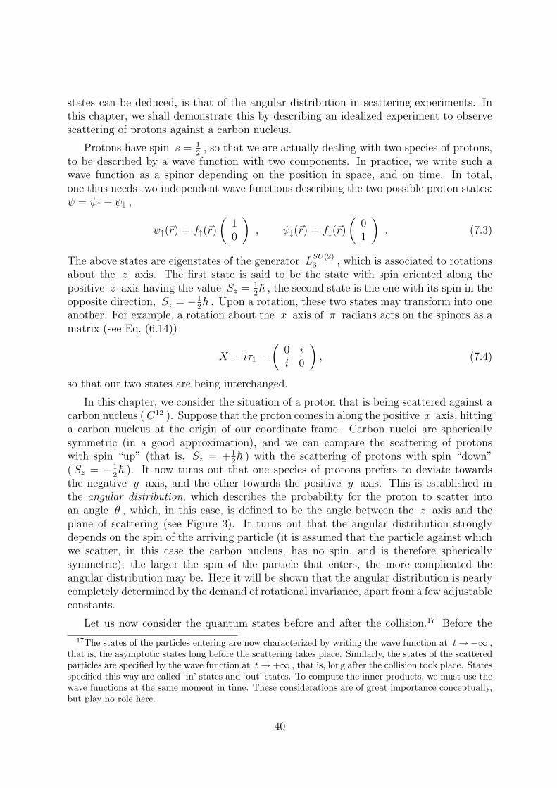
states can be deduced, is that of the angular distribution in scattering experiments. Inthis chapter, we shall demonstrate this by describing an idealized experiment to observescattering of protons against a carbon nucleus.
Protons have spin s = 12
, so that we are actually dealing with two species of protons,to be described by a wave function with two components. In practice, we write such awave function as a spinor depending on the position in space, and on time. In total,one thus needs two independent wave functions describing the two possible proton states:ψ = ψ↑ + ψ↓ ,
ψ↑(~r) = f↑(~r)(
10
), ψ↓(~r) = f↓(~r)
(01
). (7.3)
The above states are eigenstates of the generator LSU(2)3 , which is associated to rotations
about the z axis. The first state is said to be the state with spin oriented along thepositive z axis having the value Sz = 1
2~ , the second state is the one with its spin in the
opposite direction, Sz = −12~ . Upon a rotation, these two states may transform into one
another. For example, a rotation about the x axis of π radians acts on the spinors as amatrix (see Eq. (6.14))
X = iτ1 =
(0 ii 0
), (7.4)
so that our two states are being interchanged.
In this chapter, we consider the situation of a proton that is being scattered against acarbon nucleus ( C12 ). Suppose that the proton comes in along the positive x axis, hittinga carbon nucleus at the origin of our coordinate frame. Carbon nuclei are sphericallysymmetric (in a good approximation), and we can compare the scattering of protonswith spin “up” (that is, Sz = +1
2~ ) with the scattering of protons with spin “down”
( Sz = −12~ ). It now turns out that one species of protons prefers to deviate towards
the negative y axis, and the other towards the positive y axis. This is established inthe angular distribution, which describes the probability for the proton to scatter intoan angle θ , which, in this case, is defined to be the angle between the z axis and theplane of scattering (see Figure 3). It turns out that the angular distribution stronglydepends on the spin of the arriving particle (it is assumed that the particle against whichwe scatter, in this case the carbon nucleus, has no spin, and is therefore sphericallysymmetric); the larger the spin of the particle that enters, the more complicated theangular distribution may be. Here it will be shown that the angular distribution is nearlycompletely determined by the demand of rotational invariance, apart from a few adjustableconstants.
Let us now consider the quantum states before and after the collision.17 Before the
17The states of the particles entering are now characterized by writing the wave function at t → −∞ ,that is, the asymptotic states long before the scattering takes place. Similarly, the states of the scatteredparticles are specified by the wave function at t → +∞ , that is, long after the collision took place. Statesspecified this way are called ‘in’ states and ‘out’ states. To compute the inner products, we must use thewave functions at the same moment in time. These considerations are of great importance conceptually,but play no role here.
40
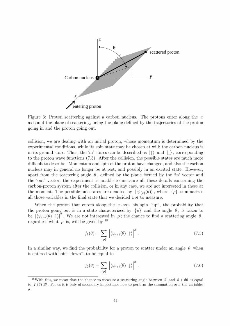
scattered proton
Carbon nucleus
entering proton
z
y
x
θ
Figure 3: Proton scattering against a carbon nucleus. The protons enter along the xaxis and the plane of scattering, being the plane defined by the trajectories of the protongoing in and the proton going out.
collision, we are dealing with an initial proton, whose momentum is determined by theexperimental conditions, while its spin state may be chosen at will; the carbon nucleus isin its ground state. Thus, the ‘in’ states can be described as |↑〉 and |↓〉 , correspondingto the proton wave functions (7.3). After the collision, the possible states are much moredifficult to describe. Momentum and spin of the proton have changed, and also the carbonnucleus may in general no longer be at rest, and possibly in an excited state. However,apart from the scattering angle θ , defined by the plane formed by the ‘in’ vector andthe ‘out’ vector, the experiment is unable to measure all these details concerning thecarbon-proton system after the collision, or in any case, we are not interested in these atthe moment. The possible out-states are denoted by | ψρ(θ)〉 , where ρ summarizesall those variables in the final state that we decided not to measure.
When the proton that enters along the x -axis his spin “up”, the probability thatthe proton going out is in a state characterized by ρ and the angle θ , is taken tobe |〈ψρ(θ) |↑〉|2 . We are not interested in ρ ; the chance to find a scattering angle θ ,regardless what ρ is, will be given by 18
f1(θ) =∑
ρ
∣∣∣〈ψρ(θ) |↑〉∣∣∣2
. (7.5)
In a similar way, we find the probability for a proton to scatter under an angle θ whenit entered with spin “down”, to be equal to
f2(θ) =∑
ρ
∣∣∣〈ψρ(θ) |↓〉∣∣∣2
. (7.6)
18With this, we mean that the chance to measure a scattering angle between θ and θ + dθ is equalto f1(θ) dθ . For us it is only of secondary importance how to perform the summation over the variablesρ .
41
Upon a rotation over π radians about the x -axis, the angle θ turns into θ+π , whilethe two spin states (7.3) of the initial proton are interchanged. This is why invarianceunder rotations implies that one must have
f1(θ) = f2(θ + π). (7.7)
We can say more, however. Consider an initial proton with spin characterized by
| ψ(a)〉 = a1 |↑〉+ a2 |↓〉. (7.8)
A procedure similar to Eqs. (7.5) and (7.6) allows us to derive that the distribution overthe angles θ is given by
f(θ) =∑
ρ
∣∣∣〈ψρ(θ) | ψ(a)〉∣∣∣2
=∑
ρ
∣∣∣a1〈ψρ(θ) |↑〉+ a2〈ψρ(θ) |↓〉∣∣∣2
= f1(θ) |a1|2 + f2(θ) |a2|2 + f12(θ) a1a∗2 + f ∗12(θ) a∗1a2 , (7.9)
where f1 en f2 are defined in (7.5) and (7.6), while the mixing term f12 is given by
f12(θ) =∑
ρ〈ψρ(θ) |↑〉 〈ψρ(θ) |↓〉∗ . (7.10)
Eq. (7.9) can also be written in matrix notation,
f(θ) =∑
α,β=1,2
F (θ)αβ a∗β aα, (7.11)
where the 2× 2 matrix F (θ) , defined by
F (θ) =
f1(θ) f ∗12(θ)
f12(θ) f2(θ)
, (7.12)
is hermitian and positive definite.
Now consider a rotation over an angle φ around the x -axis. To get the signs correct19,remember the definition (2.17) of a representation. Comparing Eq. (3.12), we see thatR(φ, 0, 0) is the rotation matrix
R(φ) = eiφL1 =
1 0 0
0 cos φ sin φ
0 − sin φ cos φ
, (7.13)
19Versions of these notes prior to 25/06/07 were not very precise at this point; we modified the notationhere.
42
which rotates the coordinates in the positive θ direction in Fig. 3. Having ψi(Rx) =Xij(φ)ψj(x) , where ψ(x) stands for 〈ψρ(θ)|ψ〉 , we find
〈ψρ(θ + φ)|ψi〉 = ψi(Rx) = Xijψj(x) = Xij〈ψρ(θ)|ψj〉 , (7.14)
and Xij is the matrix that transforms the states |↑〉 and |↓〉 :
X(φ) = eiφτ1/2 =
cos φ2
i sin φ2
i sin φ2
cos φ2
. (7.15)
Writing Eq. (7.8) as |ψ〉 = ai|ψi〉 , we find that Eq. (7.14) can be written as
〈ψρ(θ + φ)|ψ〉 = aiXij〈ψρ(θ)|ψj〉 . (7.16)
Consequently, with our definitions (7.10)—(7.12) for the matrix F (θ) , we have
F (θ + φ) = X†(φ) F (θ) X(φ) . (7.17)
This equation determines the θ dependence of the distribution. Just take θ = 0 in(7.17), so that this equation can be written as (we use X(φ)† = X(φ)−1 )
F (φ) = X(φ)−1 F (0) X(φ) . (7.18)
Elaborating this matrix equation for the individual components yields (we replace φ nowback to θ )
f1(θ) = f1 cos2 θ2
+ f2 sin2 θ2
+ i(f12 − f ∗12) cos θ2sin θ
2, (7.19)
f2(θ) = f2 cos2 θ2
+ f1 sin2 θ2− i(f12 − f ∗12) cos θ
2sin θ
2, (7.20)
f12(θ) = f12 cos2 θ2
+ f ∗12 sin2 θ2
+ i(f1 − f2) cos θ2sin θ
2, (7.21)
The θ dependence of the angular distributions thus follows completely from rotationinvariance. The functions f1(θ) en f2(θ) have exactly one maximum and one minimumin the interval −π ≤ θ ≤ π , and thus they yield exactly one preferred direction forscattering, in agreement with what was described earlier.
The angular distributions can be predicted even more precisely by making use ofyet an other symmetry. To a very good precision, Nature is also invariant under mirrorreflections in space. Under a reflection P with respect to the origin, all space coordinatesare given an extra minus sign,
~rP−→ −~r . (7.22)
Two reflections in succession yield the identity, so that what we have here is a finite groupconsisting of two elements, the space reflection P and the identity I . By adding thereflection to the rotation group SO(3) , the latter is expanded to O(3) , see the beginningof Chapter 3.
43
The generators of the rotation group do not change upon a reflection. This directlyfollows from the fact that a reflection with respect to the origin commutes with rotations,as can easily be checked. From this it follows that such a reflection acting on irreduciblerepresentations of the rotation group, must be proportional to the identity. This is whythe spin of a state does not change under reflections, and the state itself can at mostreceive a minus sign.
Consider once more the scattering of protons against carbon nuclei, and the effect ofthe O(3) matrix
Pz =
1 0 0
0 1 0
0 0 −1
. (7.23)
After this matrix, which is also a reflection since its determinant is −1 , we encounter thesame experimental situation, because the momentum of the initial proton did not change.Only the angle θ is now replaced by π−θ . Since, upon this substitution, f1(θ) en f2(θ)may not change, one must have
f1(θ) = f1(π − θ), f2(θ) = f2(π − θ) . (7.24)
This implies that f1 = f2 .
Observe that Pz can be written as the product of the reflection P = −1 and arotation over π radians about the z -axis. The reflection P does not affect the spinstates, but the rotation corresponds to
e12iπτ3 =
(i 0
0 −i
)= iτ3 . (7.25)
Consequently, we have (analogously to Eq. (7.17)) that τ3 F (π − θ) τ3 = F (θ) , whichnow also implies that f ∗12 = −f12 .
44
8. Isospin
As explained in Chapter 1, elementary particles with the same spin and similar massvalues, can be grouped in so-called multiplets. For example,
nucleon-doublet : (p, n),
pion-triplet : (π+, π0, π−) , (8.1)
Delta-quadruplet : (∆++, ∆+, ∆0, ∆−) ,
etc.
This structure can be explained by assuming that Nature is approximately invariant un-der what will be referred to as isospin rotations. Isospin rotations form a group, whoseelements can be regarded as rotations in some “internal” three-dimensional space. Thestates that correspond to the isospin multiplets transform according to (irreducible) rep-resentations of this group. Thus, the notion of isospin is analogous to the usual notion ofspin, which is connected to rotations in ordinary 3-space.
The force that binds the nucleons in an atomic nucleus, the so-called strong force, isinvariant under isospin rotations. However, the electro magnetic forces are not. This iswhy that electric charges within one multiplet are not all the same. Conservation of elec-tric charge is exact. This is associated with conservation of isospin-“angular momentum”in the 3 direction, since electric charge is described by the Gell-Mann-Nishijima relation
Q = I3 + 12Y , (8.2)
where Y is the “hyper charge”, which has the same value for all states within onemultiplet. We readily determine that Y = 1 for the nucleon and ∆ multiplets, and 0for the pion multiplet.
Now let us consider the decay of a ∆++ ,
∆++ −→ p π+ . (8.3)
For the particles involved in this decay, we have
I3 | ∆++〉 = 32| ∆++〉, I3 | p〉 = 1
2| p〉, I3 | π+〉 =| π+〉 , (8.4)
so that
I3
(| p〉 | π+〉
)=
(I3 | p〉
)| π+〉+ | p〉
(I3 | π+〉
)= 3
2| p〉 | π+〉 . (8.5)
The above equation follows from the fact that the generators Ii for a representationconsisting of the products of states, is given by the sum of the generators acting on theseparate states. Similar equations therefore hold for I+ and I− as well.
∆ particles predominantly decay into one nucleon and one pion. Because of chargeconservation, ∆++ can only decay as in Eq. (8.3). As for the other ∆ particles, the
45
situation is not so simple. Let us begin by enumerating the six different nucleon-pionstates, all being eigenstates of the I3 -operator,
I3
(| p〉 | π+〉
)= 3
2| p〉 | π+〉 ,
I3
(| p〉 | π0〉
)= 1
2| p〉 | π0〉 ,
I3
(| p〉 | π−〉
)= −1
2| p〉 | π−〉 ,
I3
(| n〉 | π+〉
)= 1
2| n〉 | π+〉 ,
I3
(| n〉 | π0〉
)= −1
2| n〉 | π0〉 ,
I3
(| n〉 | π−〉
)= −3
2| n〉 | π−〉 .
(8.6)
The fact that ∆ particles can only decay into special linear combinations of these statescan be explained by the fact that the product states (8.6) split up into two different irre-ducible representations of the isospin group. This follows immediately from an inspectionof the eigenvalues of I3 : the eigenvalues ±3
2occur only once each, while the eigenvalues
±12
occur twice each. The corresponding states must therefore form one irreducible rep-resentation with “total isospin” 3
2, and one with “total isospin” 1
2. Thus, we can write
the following decomposition of the product representation (analogously to Eq. (4.13)),
2⊗ 3 = 2⊕ 4 (8.7)
where 2 , 3 , and 4 indicate the 2-, 3- and 4-dimensional representations, associated toisospin 1
2, 1, and 3
2, respectively.
If indeed these decay processes are invariant under isospin rotations, then the decaysof the other ∆ particles can be predicted from what is known about the ∆++ decay.The operator I− turns the ∆++ state into
I− | ∆++〉 = I− | 32, 3
2〉 =
√3 | 3
2, 1
2〉 =
√3 | ∆+〉 , (8.8)
Where we used Eq. (5.22). For the nucleon pion final state, into which ∆++ decays, wefind that it transforms as
I−(| p 〉 | π+〉
)=
(I− | p 〉
)| π+〉+ | p 〉
(I− | π+〉
)
= | n〉 | π+〉+√
2 | p 〉 | π0〉 . (8.9)
Isospin invariance should now imply that | ∆+〉 , which is obtained from an isospinrotation acting on | ∆++〉 , should decay into the state obtained by applying the samerotation to the state | p 〉 | π+〉 ; this leads to the state that was obtained in Eq. (8.9),after normalization:
| ψ〉 =1√3
(| n〉 | π+〉+
√2 | p 〉 | π0〉
). (8.10)
Thus, isospin invariance implies that ∆+ must decay in the state (8.10), and we find thatthe decay probabilities for the two possible decay modes of ∆+ obey
Γ(∆+ → nπ+) : Γ(∆+ → p π0) = 1 : 2 , (8.11)
46
as is observed in the experiments.
To study the decay modes of ∆0 , we apply I− once more,
I− | ∆+〉 = 2 | ∆0〉 ,
I−(| n〉 | π+〉
)=
√2 | n〉 | π0〉 ,
I−(| p〉 | π0〉
)= | n〉 | π0〉+
√2 | p〉 | π−〉 , (8.12)
so that
I−
(| n〉 | π+〉+
√2 | p〉 | π0〉√
3
)= 2
(√2 | n〉 | π0〉+ | p〉 | π−〉√
3
). (8.13)
One concludes that the decay probabilities for the two possible decay modes of ∆0 arerelated according to
Γ(∆0 → nπ0) : Γ(∆0 → p π−) = 2 : 1 . (8.14)
Thus, we see in this example how the ratio 2 : 1 of decay rates of elementary particlescan be a consequence of invariance under the transformations forming a Lie group.
47
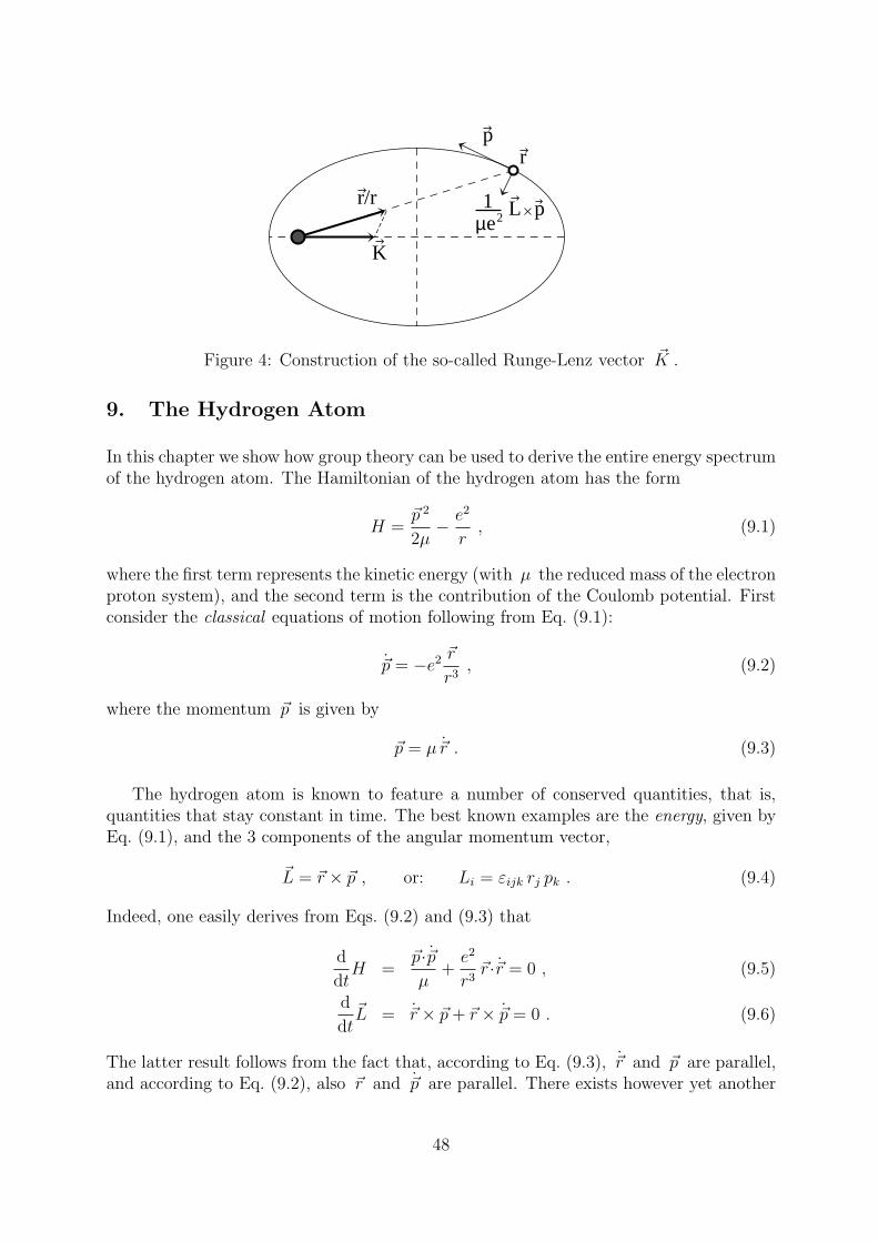
K
1
pr
r/rµe2 L p
Figure 4: Construction of the so-called Runge-Lenz vector ~K .
9. The Hydrogen Atom
In this chapter we show how group theory can be used to derive the entire energy spectrumof the hydrogen atom. The Hamiltonian of the hydrogen atom has the form
H =~p 2
2µ− e2
r, (9.1)
where the first term represents the kinetic energy (with µ the reduced mass of the electronproton system), and the second term is the contribution of the Coulomb potential. Firstconsider the classical equations of motion following from Eq. (9.1):
~p = −e2 ~r
r3, (9.2)
where the momentum ~p is given by
~p = µ ~r . (9.3)
The hydrogen atom is known to feature a number of conserved quantities, that is,quantities that stay constant in time. The best known examples are the energy, given byEq. (9.1), and the 3 components of the angular momentum vector,
~L = ~r × ~p , or: Li = εijk rj pk . (9.4)
Indeed, one easily derives from Eqs. (9.2) and (9.3) that
d
dtH =
~p·~pµ
+e2
r3~r·~r = 0 , (9.5)
d
dt~L = ~r × ~p + ~r × ~p = 0 . (9.6)
The latter result follows from the fact that, according to Eq. (9.3), ~r and ~p are parallel,and according to Eq. (9.2), also ~r and ~p are parallel. There exists however yet another
48

vector that stays constant. This is the so-called Runge-Lenz vector, defined by
~K =1
µe2~L× ~p +
~r
r. (9.7)
The fact that ~K is conserved follows from Eqs. (9.2) en (9.3), but the proof is a littlemore involved. First, we show that
d
dt~K =
1
µe2~L× ~p +
~r
r− (~r · ~r) ~r
r3
= − 1
µ
~L× ~r
r3+
r2 ~p− (~p · ~r)~rµ r3
, (9.8)
where in the first line Eq. (9.6) was used, and in the second line Eqs.(9.2) and (9.3). Next,we show that Eq. (9.8) is equal to zero by substituting Eq. (9.4), so that
d
dt~K =
1
µ r3
−(~r × ~p)× ~r + r2 ~p− (~r · ~p)~r
. (9.9)
Using the relation
(~a×~b)× ~c = (~c · ~a)~b− (~c ·~b)~a , (9.10)
we subsequently show that Eq. (9.9) is equal to zero, so that ~K is indeed a constantvector.
The Runge-Lenz vector enjoys a number of other interesting properties. Using thedefinitions and the elementary relations from vector analysis, we find
~K ·~L = 0 , (9.11a)
~K2 =
(1
µe2
)2
(~L× ~p )2 +2
µ e2 r(~L× ~p)·~r + 1
=
(1
µe2
)2
~L2 ~p 2 − 2
µ e2 r~L 2 + 1
=2H
µe4~L2 + 1 . (9.11b)
For the elliptical orbit of a classical particle, the Runge-Lenz vector ~K in fact pointsinto the direction of the semi major axis of the ellipse, see the illustration in Figure 4.The length of ~K is the excentricity ε of the ellipse.
In quantum mechanics, the vectors ~r en ~p are operators, obeying Heisenberg’s com-mutation relations,
[pi, rj] = −i~ δij ,
[ri, rj] = [pi, pj] = 0 . (9.12)
49
In the coordinate representation, we describe states in terms of wave functions of the coor-dinates ri . The coordinate operator then acts trivially on the wave function, multiplyingit by the value of the coordinate, whereas the momentum operators are given by
~p =~i
∂
∂~r. (9.13)
Naturally, also H , ~L and ~K are operators now, but the definition of ~K presents uswith a new problem, since ~p and ~L do not commute,
[Li, pj] = i~ εijk pk ,
[Li, rj] = i~ εijk rk . (9.14)
which follows directly from Eqs. (9.4) and (9.12) using the commutation relation
[A,BC] = [A,B] C + B [A,C] . (9.15)
In view of Eq. (9.14), it is not obvious in which order the operators ~L en ~p have to be
placed in the definition of Eq. (9.7) for ~K .20 We now propose the following choice for
the quantum mechanical definition of ~K :
~K =1
2µe2
(~L× ~p− ~p× ~L
)+
~r
r. (9.16)
It is clear that this definition would boil down to Eq. (9.7) if ~L and ~p would commute.
With this particular choice, the operator ~K is hermitian.
In quantum mechanics, conserved quantities commute with the Hamiltonian. Letus first check this for the operators ~L . Using the commutation relations (9.14), andEq. (9.15), we readily derive that
[Li, H] = 0 , (9.17)
[Li, Lj] = i~ εijk Lk . (9.18)
Eq. (9.17) indicates that Li is conserved. Eq. (9.18) shows that angular momentumoperators obey the same commutation relations as the operators in Eq. (3.28) for thethree-dimensional rotation group21.
By way of illustration, we give the explicit derivation of Eq. (9.18):
[Li, Lj] = εjkl [Li, rk pl]
= εjkl ([Li, rk] pl + rk [Li, pl])
= i~ εjkl (εikm rm pl + εilm rk pm)
= i~ (εjlk εimk + εjmk εikl) rm pl
= i~ εijk εkml rm pl , (9.19)
20The reader may wish to check that this problem does not arise in the definitions (9.1) and (9.4) ofH and ~L .
21Apart from the factors ~ ; the operators Li in this chapter include the constant ~ as commonlyused in quantum mechanics.
50
Where successively Eqs. (9.4), (9.15) and (9.14) were used; furthermore, indices wererenamed, and Eq. (3.33) for ε tensors was employed.
In a similar fashion we can determine commutators containing the operators ~K . First,by using Eq. (9.13), we verify that
[~p,
1
r
]=~i
(∂
∂~r
1
r− 1
r
∂
∂~r
)= i~
~r
r3. (9.20)
Subsequently, we derive that
[Li, Kj] = i~ εijk Kk (9.21)
(a property that also follows from the fact that the Ki form a vector),
[Ki, pj] =i~µe2
(pipj − p2 δij) +i~r3
(r2δij − rirj) , (9.22)
[Ki,
1
r
]=
i~2µe2
εijkLjrk + rkLj
r3. (9.23)
Using eqs. (9.22) and (9.23), it is now not difficult to prove that ~K commutes with theHamiltonian,
[ ~K, H] = 0 . (9.24)
Finally, we can conclude from the Jacobi identity,
[[A,B], C] + [[B, C], A] + [[C,A], B] = 0 , (9.25)
that also [Ki, Kj] must commute with the Hamiltonian, and is therefore conserved. Acomputation shows that this commutator does not give us a new conserved quantity, butit is a product of two conserved quantities that we already had,22
[Ki, Kj] = i~ εijk Lk
(−2H
µe4
). (9.26)
Since Lk and H commute, the order of these operators is immaterial.
Herewith, all relevant commutators have been determined. Next, we must establishwhether the classical relations (9.11) remain valid for the case that ~K and ~L are oper-ators. For the first equation, we find
~K · ~L = ~L · ~K =1
2µe2
~L · (~L× ~p)− ~L · (p× ~L)
+
~L · ~rr
. (9.27)
22On general grounds one can prove that the hydrogen atom cannot have more than 5 independentconserved quantities. For instance, one can choose the components of the angular momentum and thetwo coordinates of the Runge-Lenz vector that are orthogonal to ~L .
51
Since ~L · ~r = 0 (this continues to hold true in quantum mechanics as one easily checks),only the first two terms contribute, proportional to
εijk Li (Ljpk − pjLk) = εijk (2 Li Lj pk − i~εjkl Li pl) , (9.28)
where use was made of Eq. (9.14) to write pi at the right of the operators Li . Using
Eq. (9.18) we write the first term proportional to εijk εijl Ll pk ∝ ~L · ~p = 0 ; the secondterm vanishes for the same reason, so that we find the same result as before,
~K · ~L = 0 . (9.29)
Eq. (9.11b) no longer holds in the quantum mechanical case, and the exchange of twooperators leads to extra terms. The correct result, which requires some more calculations,takes the following form,
~K2 =2H
µe4(~L 2 + ~2) + 1 . (9.30)
In the limit ~→ 0 this result agrees with (9.11b).
The above results now enable us to determine the energy spectrum of the hydrogenatom. Consider the eigenstates of H , obeying
H | ψ〉 = E | ψ〉 , (9.31)
where the energy E will be assumed to be negative, E < 0 , so that we are dealing withbound states. Since the operators Li en Ki commute with the Hamiltonian, all statesLi | ψ〉 and Ki | ψ〉 also solve the Schrodinger equation (9.31). Within the set (9.31),the operators Li and Ki may be seen to act as the generators of a Lie group, becausetheir commutators are linear combinations of the Li and Ki themselves. Indeed, theygenerate the Lie group of all transformations that leave the energy E invariant. TheHamiltonian is a Casimir operator.
In order to analyze the mathematical structure of this Lie group, define the followingtwo linear combinations of the operators ~L and ~K ,23
~L± =1
2
(~L±
õ e4
−2E~K
). (9.32)
These operators commute with the Hamiltonian,
[L±i , H] = 0 . (9.33)
23The fact that E is negative, ensures that the argument of the square root in these definitions ispositive.Note that ~L+ and ~L− each are vectors, out of which the ladder operators L+
± and L−± of Chapter 5can be constructed.
52
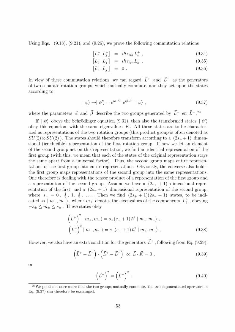
Using Eqs. (9.18), (9.21), and (9.26), we prove the following commutation relations
[L+
i , L+j
]= i~ εijk L+
k , (9.34)[L−i , L−j
]= i~ εijk L−k , (9.35)[
L+i , L−j
]= 0 . (9.36)
In view of these commutation relations, we can regard ~L+ and ~L− as the generatorsof two separate rotation groups, which mutually commute, and they act upon the statesaccording to
| ψ〉 →| ψ′〉 = ei~α·~L+
ei~β·~L− | ψ〉 , (9.37)
where the parameters ~α and ~β describe the two groups generated by ~L+ en ~L− .24
If | ψ〉 obeys the Schrodinger equation (9.31), then also the transformed states | ψ′〉obey this equation, with the same eigenvalues E . All these states are to be character-ized as representations of the two rotation groups (this product group is often denoted asSU(2)⊗SU(2) ). The states should therefore transform according to a (2s+ +1) dimen-sional (irreducible) representation of the first rotation group. If now we let an elementof the second group act on this representation, we find an identical representation of thefirst group (with this, we mean that each of the states of the original representation staysthe same apart from a universal factor). Thus, the second group maps entire represen-tations of the first group into entire representations. Obviously, the converse also holds:the first group maps representations of the second group into the same representations.One therefore is dealing with the tensor product of a representation of the first group anda representation of the second group. Assume we have a (2s+ + 1) dimensional repre-sentation of the first, and a (2s− + 1) dimensional representation of the second group,where s± = 0 , 1
2, 1, 3
2, . . . . Then we find (2s+ + 1)(2s− + 1) states, to be indi-
cated as | m+, m−〉 , where m± denotes the eigenvalues of the components L±3 , obeying−s± ≤ m± ≤ s± . These states obey
(~L+
)2
| m+,m−〉 = s+(s+ + 1) ~2 | m+,m−〉 ,(~L−
)2
| m+,m−〉 = s−(s− + 1) ~2 | m+,m−〉 , (9.38)
However, we also have an extra condition for the generators ~L± , following from Eq. (9.29):
(~L+ + ~L−
)·(~L+ − ~L−
)∝ ~L · ~K = 0 , (9.39)
or
(~L+
)2
=(~L−
)2
. (9.40)
24We point out once more that the two groups mutually commute. the two exponentiated operators inEq. (9.37) can therefore be exchanged.
53
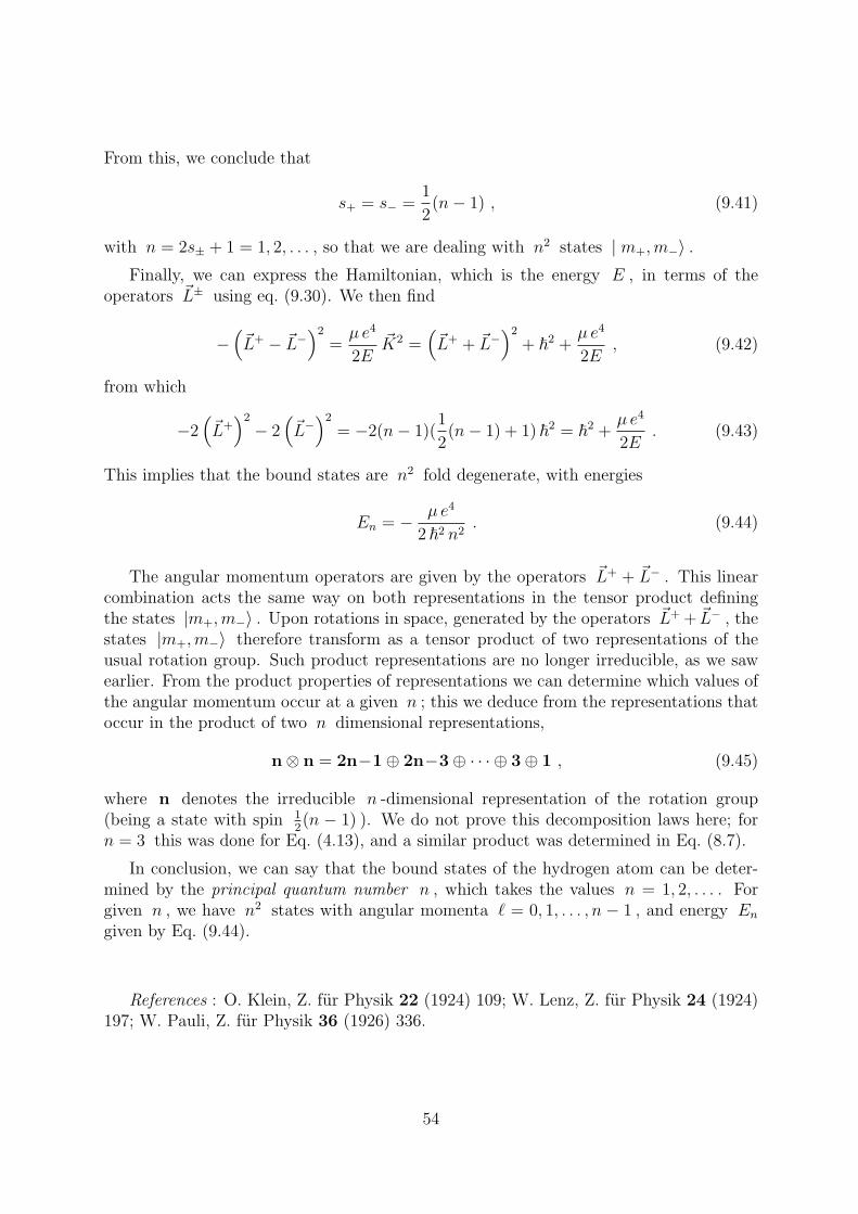
From this, we conclude that
s+ = s− =1
2(n− 1) , (9.41)
with n = 2s± + 1 = 1, 2, . . . , so that we are dealing with n2 states | m+,m−〉 .
Finally, we can express the Hamiltonian, which is the energy E , in terms of theoperators ~L± using eq. (9.30). We then find
−(~L+ − ~L−
)2
=µ e4
2E~K2 =
(~L+ + ~L−
)2
+ ~2 +µ e4
2E, (9.42)
from which
−2(~L+
)2
− 2(~L−
)2
= −2(n− 1)(1
2(n− 1) + 1) ~2 = ~2 +
µ e4
2E. (9.43)
This implies that the bound states are n2 fold degenerate, with energies
En = − µ e4
2 ~2 n2. (9.44)
The angular momentum operators are given by the operators ~L+ + ~L− . This linearcombination acts the same way on both representations in the tensor product definingthe states |m+,m−〉 . Upon rotations in space, generated by the operators ~L+ + ~L− , thestates |m+,m−〉 therefore transform as a tensor product of two representations of theusual rotation group. Such product representations are no longer irreducible, as we sawearlier. From the product properties of representations we can determine which values ofthe angular momentum occur at a given n ; this we deduce from the representations thatoccur in the product of two n dimensional representations,
n⊗ n = 2n−1⊕ 2n−3⊕ · · · ⊕ 3⊕ 1 , (9.45)
where n denotes the irreducible n -dimensional representation of the rotation group(being a state with spin 1
2(n − 1) ). We do not prove this decomposition laws here; for
n = 3 this was done for Eq. (4.13), and a similar product was determined in Eq. (8.7).
In conclusion, we can say that the bound states of the hydrogen atom can be deter-mined by the principal quantum number n , which takes the values n = 1, 2, . . . . Forgiven n , we have n2 states with angular momenta ` = 0, 1, . . . , n − 1 , and energy En
given by Eq. (9.44).
References : O. Klein, Z. fur Physik 22 (1924) 109; W. Lenz, Z. fur Physik 24 (1924)197; W. Pauli, Z. fur Physik 36 (1926) 336.
54
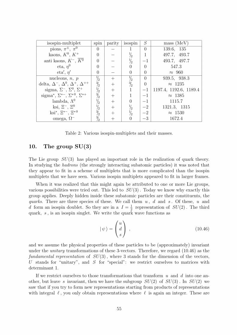
isospin-multiplet spin parity isospin S mass (MeV)pions, π±, π0 0 − 1 0 139.6, 135kaons, K0, K+ 0 − 1/2 1 497.7, 493.7
anti kaons, K−, K0 0 − 1/2 −1 493.7, 497.7eta, η0 0 − 0 0 547.3eta′, η′ 0 − 0 0 ≈ 960
nucleons, n, p 1/2 + 1/2 0 939.5, 938.3delta, ∆−, ∆0, ∆+, ∆++ 3/2 + 3/2 0 ≈ 1235
sigma, Σ−, Σ0, Σ+ 1/2 + 1 −1 1197.4, 1192.6, 1189.4sigma∗, Σ∗−, Σ∗ 0, Σ∗+ 3/2 + 1 −1 ≈ 1385
lambda, Λ0 1/2 + 0 −1 1115.7ksi, Ξ−, Ξ0 1/2 + 1/2 −2 1321.3, 1315
ksi∗, Ξ∗−, Ξ∗ 0 3/2 + 1/2 −2 ≈ 1530omega, Ω− 3/2 + 0 −3 1672.4
Table 2: Various isospin-multiplets and their masses.
10. The group SU(3)
The Lie group SU(3) has played an important role in the realization of quark theory.In studying the hadrons (the strongly interacting subatomic particles) it was noted thatthey appear to fit in a scheme of multiplets that is more complicated than the isospinmultiplets that we have seen. Various isospin multiplets appeared to fit in larger frames.
When it was realized that this might again be attributed to one or more Lie groups,various possibilities were tried out. This led to SU(3) . Today we know why exactly thisgroup applies. Deeply hidden inside these subatomic particles are their constituents, thequarks. There are three species of these. We call them u , d and s . Of these, u andd form an isospin doublet. So they are in a I = 1
2representation of SU(2) . The third
quark, s , is an isospin singlet. We write the quark wave functions as
|ψ 〉 =
uds
, (10.46)
and we assume the physical properties of these particles to be (approximately) invariantunder the unitary transformations of these 3-vectors. Therefore, we regard (10.46) as thefundamental representation of SU(3) , where 3 stands for the dimension of the vectors,U stands for “unitary”, and S for “special”: we restrict ourselves to matrices withdeterminant 1.
If we restrict ourselves to those transformations that transform u and d into one an-other, but leave s invariant, then we have the subgroup SU(2) of SU(3) . In SU(2) wesaw that if you try to form new representations starting from products of representationswith integral ` , you only obtain representations where ` is again an integer. These are
55
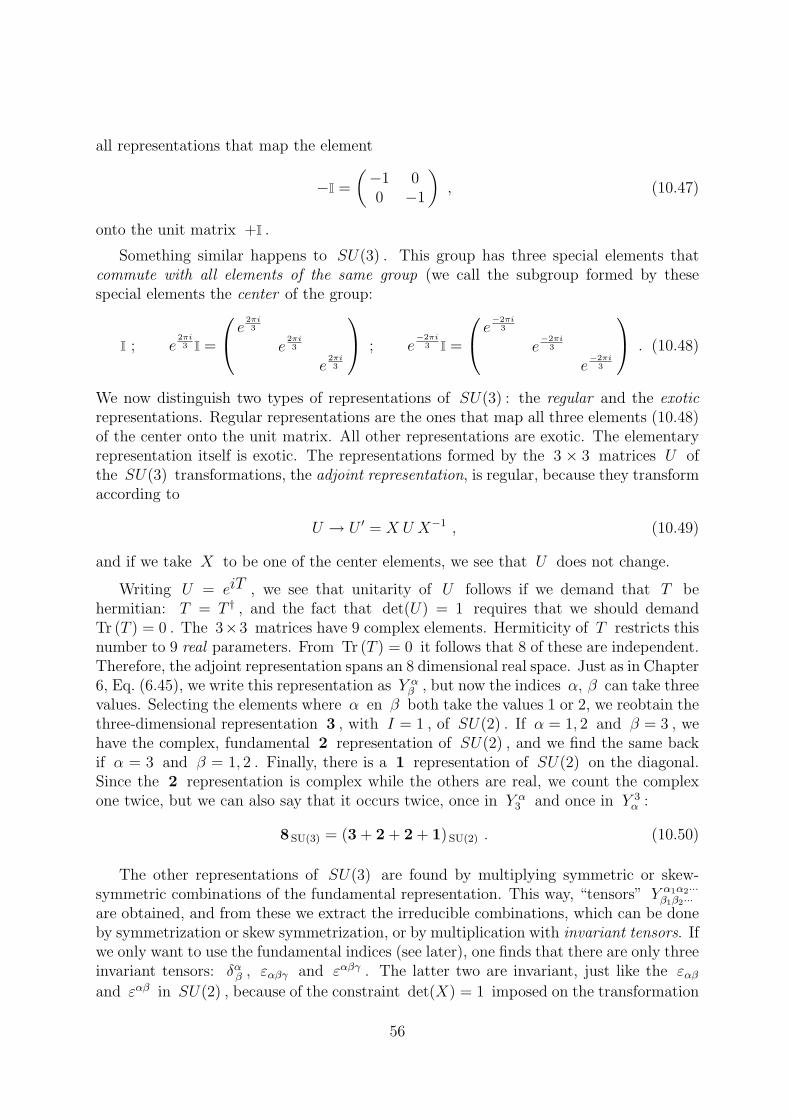
all representations that map the element
−I =
(−1 00 −1
), (10.47)
onto the unit matrix +I .
Something similar happens to SU(3) . This group has three special elements thatcommute with all elements of the same group (we call the subgroup formed by thesespecial elements the center of the group:
I ; e2πi3 I =
e2πi3
e2πi3
e2πi3
; e
−2πi3 I =
e−2πi
3
e−2πi
3
e−2πi
3
. (10.48)
We now distinguish two types of representations of SU(3) : the regular and the exoticrepresentations. Regular representations are the ones that map all three elements (10.48)of the center onto the unit matrix. All other representations are exotic. The elementaryrepresentation itself is exotic. The representations formed by the 3 × 3 matrices U ofthe SU(3) transformations, the adjoint representation, is regular, because they transformaccording to
U → U ′ = X U X−1 , (10.49)
and if we take X to be one of the center elements, we see that U does not change.
Writing U = eiT , we see that unitarity of U follows if we demand that T behermitian: T = T † , and the fact that det(U) = 1 requires that we should demandTr (T ) = 0 . The 3×3 matrices have 9 complex elements. Hermiticity of T restricts thisnumber to 9 real parameters. From Tr (T ) = 0 it follows that 8 of these are independent.Therefore, the adjoint representation spans an 8 dimensional real space. Just as in Chapter6, Eq. (6.45), we write this representation as Y α
β , but now the indices α, β can take threevalues. Selecting the elements where α en β both take the values 1 or 2, we reobtain thethree-dimensional representation 3 , with I = 1 , of SU(2) . If α = 1, 2 and β = 3 , wehave the complex, fundamental 2 representation of SU(2) , and we find the same backif α = 3 and β = 1, 2 . Finally, there is a 1 representation of SU(2) on the diagonal.Since the 2 representation is complex while the others are real, we count the complexone twice, but we can also say that it occurs twice, once in Y α
3 and once in Y 3α :
8SU(3) = (3 + 2 + 2 + 1)SU(2) . (10.50)
The other representations of SU(3) are found by multiplying symmetric or skew-symmetric combinations of the fundamental representation. This way, “tensors” Y α1α2···
β1β2···are obtained, and from these we extract the irreducible combinations, which can be doneby symmetrization or skew symmetrization, or by multiplication with invariant tensors. Ifwe only want to use the fundamental indices (see later), one finds that there are only threeinvariant tensors: δα
β , εαβγ and εαβγ . The latter two are invariant, just like the εαβ
and εαβ in SU(2) , because of the constraint det(X) = 1 imposed on the transformation
56
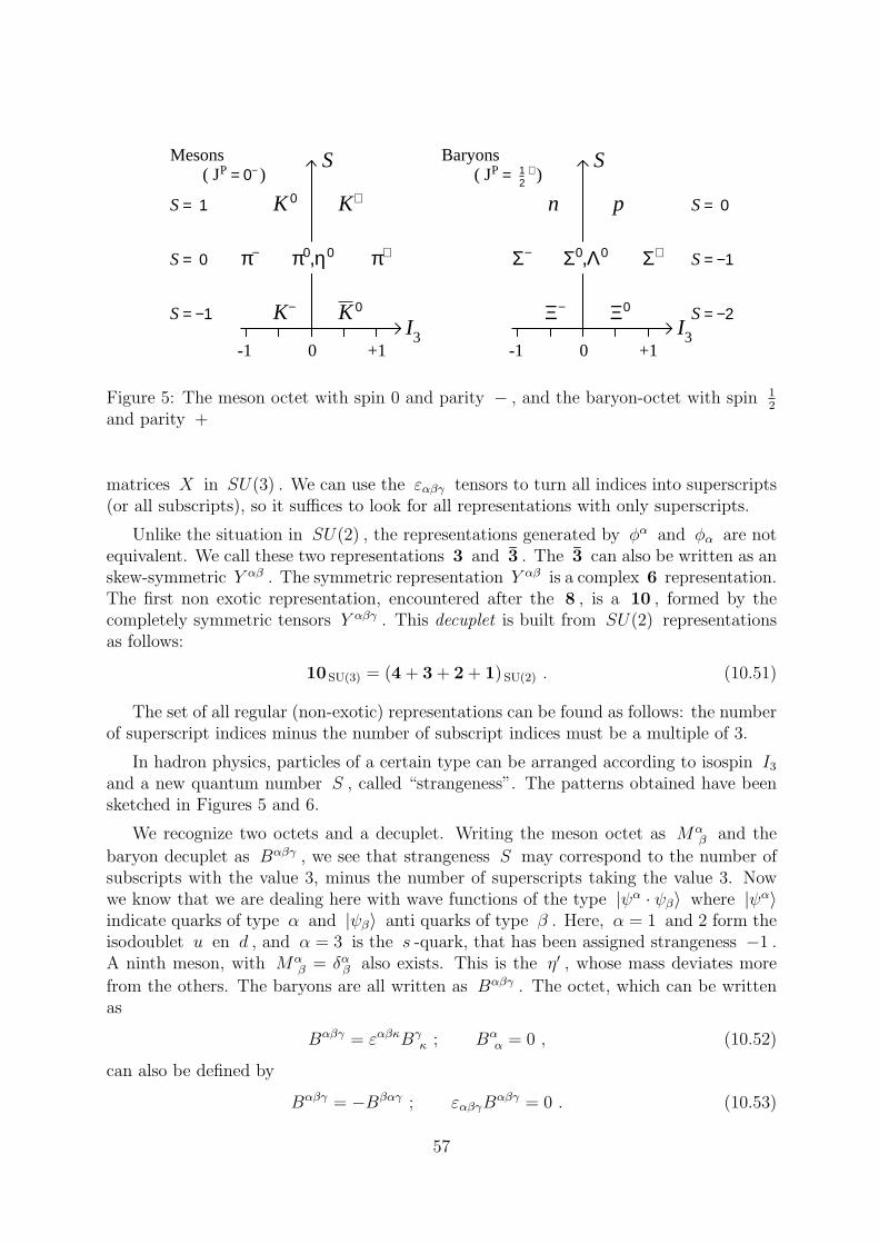
S
S = 1
S = 0
S = −1
K 0 K+
π− π0,η0 π+
K− K 0
I3+10-1
Mesons( JP = 0− )
S
S = 0
S = −1
S = −2
pn
Σ− Σ0,Λ0 Σ+
Ξ− Ξ0
I3+10-1
Baryons( JP = 12
+ )
Figure 5: The meson octet with spin 0 and parity − , and the baryon-octet with spin 12
and parity +
matrices X in SU(3) . We can use the εαβγ tensors to turn all indices into superscripts(or all subscripts), so it suffices to look for all representations with only superscripts.
Unlike the situation in SU(2) , the representations generated by φα and φα are notequivalent. We call these two representations 3 and 3 . The 3 can also be written as anskew-symmetric Y αβ . The symmetric representation Y αβ is a complex 6 representation.The first non exotic representation, encountered after the 8 , is a 10 , formed by thecompletely symmetric tensors Y αβγ . This decuplet is built from SU(2) representationsas follows:
10 SU(3) = (4 + 3 + 2 + 1)SU(2) . (10.51)
The set of all regular (non-exotic) representations can be found as follows: the numberof superscript indices minus the number of subscript indices must be a multiple of 3.
In hadron physics, particles of a certain type can be arranged according to isospin I3
and a new quantum number S , called “strangeness”. The patterns obtained have beensketched in Figures 5 and 6.
We recognize two octets and a decuplet. Writing the meson octet as Mαβ and the
baryon decuplet as Bαβγ , we see that strangeness S may correspond to the number ofsubscripts with the value 3, minus the number of superscripts taking the value 3. Nowwe know that we are dealing here with wave functions of the type |ψα · ψβ〉 where |ψα〉indicate quarks of type α and |ψβ〉 anti quarks of type β . Here, α = 1 and 2 form theisodoublet u en d , and α = 3 is the s -quark, that has been assigned strangeness −1 .A ninth meson, with Mα
β = δαβ also exists. This is the η′ , whose mass deviates more
from the others. The baryons are all written as Bαβγ . The octet, which can be writtenas
Bαβγ = εαβκBγκ ; Bα
α = 0 , (10.52)
can also be defined by
Bαβγ = −Bβαγ ; εαβγBαβγ = 0 . (10.53)
57
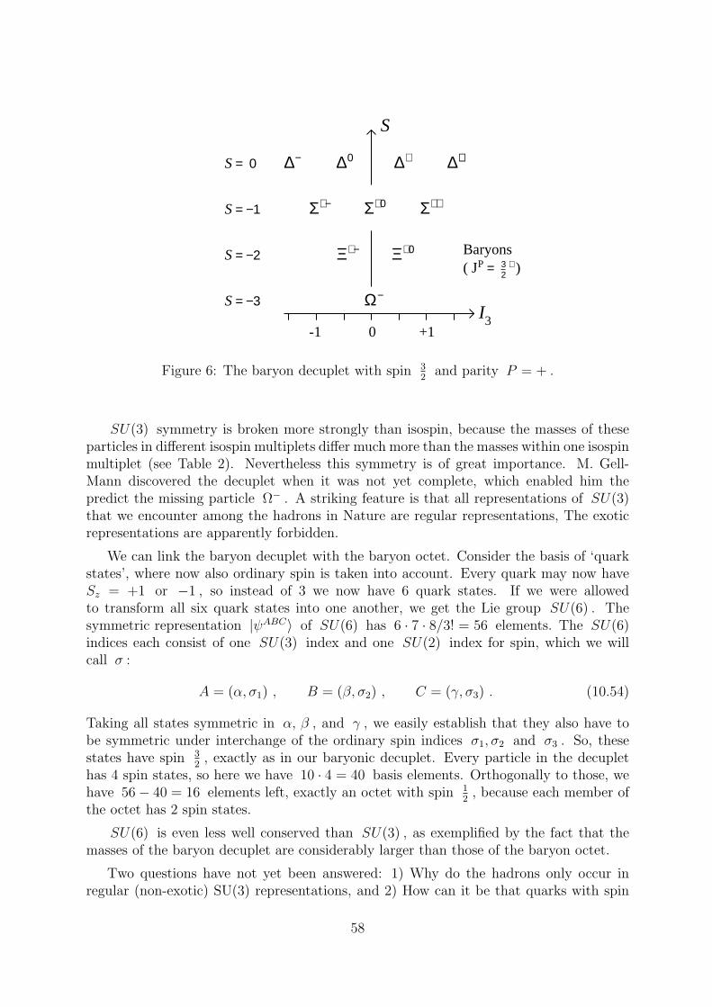
S
S = 0
S = −1
S = −2
S = −3
∆− ∆0 ∆+ ∆++
Σ∗− Σ∗0 Σ∗+
Ξ∗− Ξ∗0
Ω−
I3+10-1
Baryons( JP = 32
+ )
Figure 6: The baryon decuplet with spin 32
and parity P = + .
SU(3) symmetry is broken more strongly than isospin, because the masses of theseparticles in different isospin multiplets differ much more than the masses within one isospinmultiplet (see Table 2). Nevertheless this symmetry is of great importance. M. Gell-Mann discovered the decuplet when it was not yet complete, which enabled him thepredict the missing particle Ω− . A striking feature is that all representations of SU(3)that we encounter among the hadrons in Nature are regular representations, The exoticrepresentations are apparently forbidden.
We can link the baryon decuplet with the baryon octet. Consider the basis of ‘quarkstates’, where now also ordinary spin is taken into account. Every quark may now haveSz = +1 or −1 , so instead of 3 we now have 6 quark states. If we were allowedto transform all six quark states into one another, we get the Lie group SU(6) . Thesymmetric representation |ψABC〉 of SU(6) has 6 · 7 · 8/3! = 56 elements. The SU(6)indices each consist of one SU(3) index and one SU(2) index for spin, which we willcall σ :
A = (α, σ1) , B = (β, σ2) , C = (γ, σ3) . (10.54)
Taking all states symmetric in α, β , and γ , we easily establish that they also have tobe symmetric under interchange of the ordinary spin indices σ1, σ2 and σ3 . So, thesestates have spin 3
2, exactly as in our baryonic decuplet. Every particle in the decuplet
has 4 spin states, so here we have 10 · 4 = 40 basis elements. Orthogonally to those, wehave 56− 40 = 16 elements left, exactly an octet with spin 1
2, because each member of
the octet has 2 spin states.
SU(6) is even less well conserved than SU(3) , as exemplified by the fact that themasses of the baryon decuplet are considerably larger than those of the baryon octet.
Two questions have not yet been answered: 1) Why do the hadrons only occur inregular (non-exotic) SU(3) representations, and 2) How can it be that quarks with spin
58

12
are in a symmetric wave function; having spin 12
one would have expected that quarksare fermions, which should occur only in completely skew-symmetric wave functions, inview of Pauli’s exclusion principle. The answer to both questions is that quarks carry yetanother, ‘internal’ quantum number, called color, which again can take three values. Thecolor theory can explain the nature of the forces between the quarks. Attractive forcesbetween quarks with different values for the color index are so great that these colorsmust neutralize each other completely. This theory will not be further explained here,but it is known to imply that all hadrons must form a color singlet representation. Thewave function must therefore be completely skew-symmetric under exchanges of the colorindices. In agreement with Pauli’s principle, the entire wave functions of the hadronsare completely skew-symmetric under the interchange of two quarks. This leaves us withcompletely symmetric wave functions when only two SU(6) indices are interchanged.
To describe the generators of an SU(3) transformation, we use the hermitian matricesλ a, α = 1, · · · , 8 :
X = exp(12iθ aλ a) . (10.55)
λ a , called the Gell-Mann matrices, are a generalization of the SU(2) matrices τi :
λ 1 =
0 1 ·1 0 ·· · ·
λ 2 =
0 −i ·i 0 ·· · ·
λ 3 =
1 0 ·0 −1 ·· · ·
λ 4 =
0 · 1· · ·1 · 0
λ 5 =
0 · −i· · ·i · 0
λ 6 =
· · ·· 0 1· 1 0
λ 7 =
· · ·· 0 −i· i 0
λ 8 =
1√3
1 0 00 1 00 0 −2
(10.56)
The λ a are normalized according to
Tr (λ a λ b) = 2δab , (10.57)
and they obey the commutation relations
[12λ a,
12λ b] = ifabc(
12λ c) . (10.58)
The list of the structure constants fabc is
f123 = 1
f147 = f246 = f257 = f345 = f516 = f637 = 12
f458 = f678 = 12
√3 ; (10.59)
the remaining ones follow from the complete antisymmetry of these coefficients:
fabc = fbca = −fbac , etc. (10.60)
59
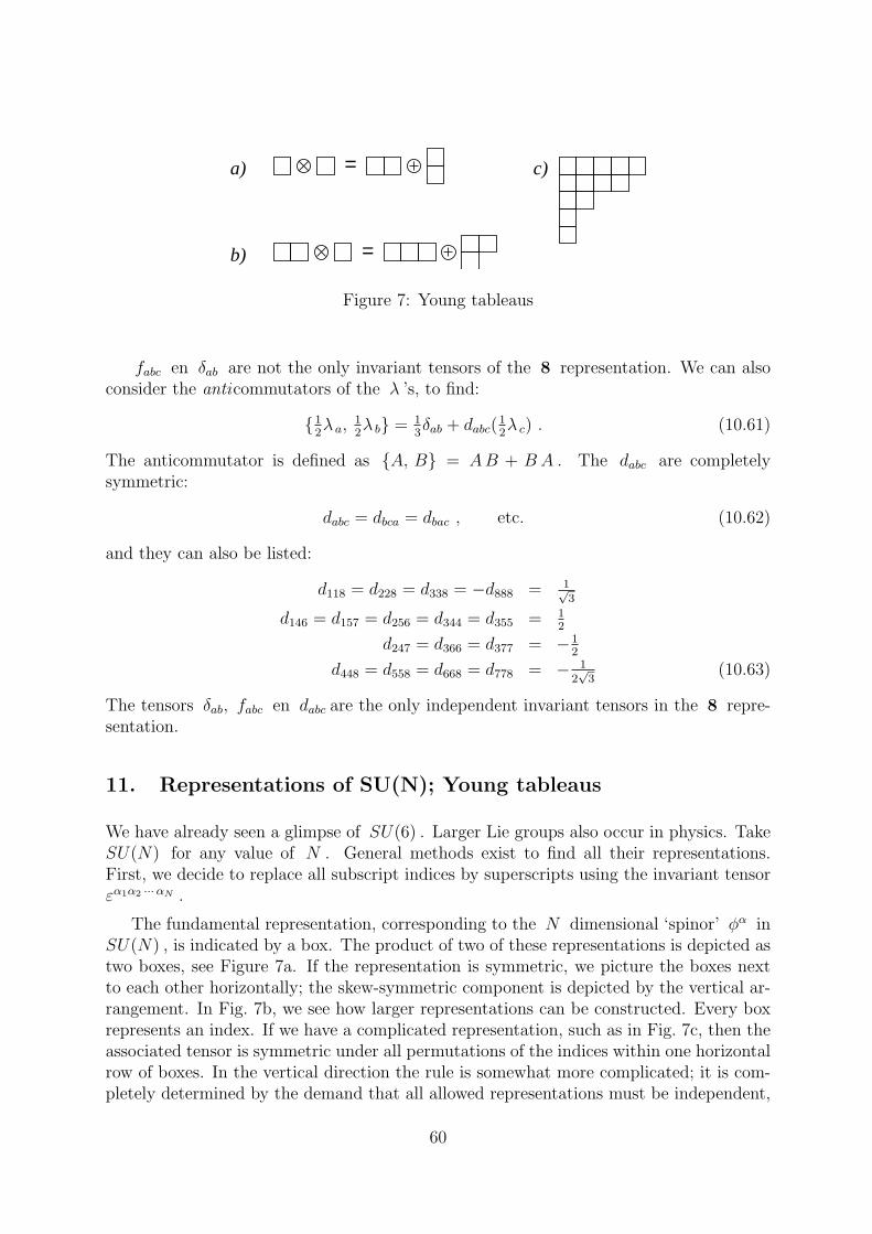
= c)
b)
a)
=
Figure 7: Young tableaus
fabc en δab are not the only invariant tensors of the 8 representation. We can alsoconsider the anticommutators of the λ ’s, to find:
12λ a,
12λ b = 1
3δab + dabc(
12λ c) . (10.61)
The anticommutator is defined as A, B = AB + B A . The dabc are completelysymmetric:
dabc = dbca = dbac , etc. (10.62)
and they can also be listed:
d118 = d228 = d338 = −d888 = 1√3
d146 = d157 = d256 = d344 = d355 = 12
d247 = d366 = d377 = −12
d448 = d558 = d668 = d778 = − 12√
3(10.63)
The tensors δab, fabc en dabc are the only independent invariant tensors in the 8 repre-sentation.
11. Representations of SU(N); Young tableaus
We have already seen a glimpse of SU(6) . Larger Lie groups also occur in physics. TakeSU(N) for any value of N . General methods exist to find all their representations.First, we decide to replace all subscript indices by superscripts using the invariant tensorεα1α2 ···αN .
The fundamental representation, corresponding to the N dimensional ‘spinor’ φα inSU(N) , is indicated by a box. The product of two of these representations is depicted astwo boxes, see Figure 7a. If the representation is symmetric, we picture the boxes nextto each other horizontally; the skew-symmetric component is depicted by the vertical ar-rangement. In Fig. 7b, we see how larger representations can be constructed. Every boxrepresents an index. If we have a complicated representation, such as in Fig. 7c, then theassociated tensor is symmetric under all permutations of the indices within one horizontalrow of boxes. In the vertical direction the rule is somewhat more complicated; it is com-pletely determined by the demand that all allowed representations must be independent,
60
so that two tensors that are described by different Young tableaus are always orthogonalto one another. It then turns out that we arrive at the following rule:
i All independent, irreducible representations of SU(N) can be distinguished by thefact that they have different Young tableaus, and every Young tableau representsone irreducible representation, provided that:
ii Every horizontal row in a Young tableau may not have more boxes than the rowabove it, and every column may not have more boxes than the column left of it.
iii There cannot be more than N − 1 rows, so the columns may not have more thanN − 1 boxes.
A typical example is the Young tableau of Fig. 7c.
12. Beyond these notes
There is a large amount of literature on Lie groups. The problem of classifying all in-equivalent Lie groups has been solved (W. Killing and E. Cartan). One first defines thesimple Lie groups, which are the Lie groups that cannot be written as the product of twonon-trivial mutually commuting Lie groups. Then it was found that there are four infiniteseries of these:
The groups An = SU(n + 1) ; n ≥ 1 ,
The groups Bn = SO(2n + 1) ; n ≥ 2 ,
The groups Cn = Sp(2n) , n ≥ 3 ,
The groups Dn = SO(2n) , n ≥ 4 ;
n may take values smaller than the limits indicated, but these groups are not independentof the others given, for instance: the algebra of SO(3) coincides with that of SU(2) , aswas described in these notes. We write SO(3) ∼= SU(2) . Similarly, one has SO(4) ∼=SO(3)⊗ SO(3) and SO(6) ∼= SU(4) .
The groups Sp(2n) are the so-called symplectic groups.
Besides these regular series, there are five more simple Lie groups that are not in oneof these series, called the exceptional groups, E6, E7, E8, F4 , and G2 . The E8 algebrais the largest and most complicated of these exceptional cases. This group is so large thatit could easily encompass all known particles and fields, and since it also plays a role insuper string theories, it receives a lot of interest from physicists.
The Lie algebra can also be extended to algebras where, at various places, the com-mutators are replaced by anticommutators. One then gets the graded Lie groups. Theseplay a role in supersymmetric particle theories.
61

Appendix A
Summary of the properties of matrices
A square matrix of dimension n is a table of n× n elements aij :
A =
a11 a12 · · · a1n
a21 a22 · · · a2n...
......
an1 an2 · · · ann
.
The matrix elements aij are (possibly complex) numbers. Suppose we have an othern× n matrix B with elements bij .
Definition: The sum of two matrices A and B is a matrix C with matrix elementsgiven by
cij = aij + bij . (A.1)
Their difference C ′ is given by the matrix elements c′ij = aij − bij . We write:
C = A + B, or C ′ = A−B .
From Eq. (A.1) it follows that the summation is commutative: A + B = B + A .
Definition: The product of the matrices A and B is a matrix C with matrix elementscij given by
cij =n∑
k=1
aikbkj. (A.2)
We write:C = AB . (A.3)
Explanation: Eq. (A.2) defines the matrix elements cij if aij and bij are given. Sinceaij and bij are ordinary numbers, it does not matter in which order they are written.This does not hold, however, for products of matrices, where in general C = A B 6= B A .Note that C ′ = BA is a matrix whose elements are given by
c′ij =∑
k
bikakj , (A.4)
which differs from Eq. (A.2). We say that matrix multiplication is non commutative. Itis associative: A(BC) = (AB)C .
Definition: The commutator of two matrices A and B is given by
[A,B] ≡ AB −BA . (A.5)
62
We say that A and B commute if the commutator is equal to zero.
Definition: The product of a (possibly complex) number x with a matrix A is amatrix B with elements:
bij = x aij . (A.6)
Notation:
B = xA . (A.7)
From Eq. (A.6), it follows thatB2 = x2A2 ,
since ∑
k
bikbkj = x2∑
k
aikakj .
Definition: The unit matrix 1 is defined as
1 =
1 0 · · · 00 1 · · · 0...
.... . .
...0 0 · · · 1
,
and gives 1A = A1 = A for every matrix A .For every n×n matrix we can define its determinant, being a (possibly complex) number.It is defined recursively by taking out one of its rows, say the ith row:
Det(A) =n∑
k=1
aik(−1)k+iDet(A(i, k)) , (A.8)
where the (n− 1)× (n− 1) matrix A(i, k) is obtained from A by removing the ith rowand the kth column. The determinant of a 0× 0 matrix is 1.
Many properties of determinants are easy to derive: if C = AB then
Det(C) = Det(AB) = Det(A) Det(B) . (A.9)
If C = xA with x a number and A an n× n matrix,
Det(C) = Det(xA) = xnDet(A) . (A.10)
Furthermore: the inverse of a matrix A is a matrix B such that BA = AB = 1 .Notation: B = A−1 . The matrix elements of B are (note: A(j, i) , not A(i, j) ):
bij =(−1)i+jDet(A(j, i))
Det(A). (A.11)
63
from this, it follows that a matrix A has an inverse if Det(A) 6= 0 . An other definitionof the determinant makes use of the ε symbols, defined by
εi1···in = 0 if in i1 . . . in two or more of the indices are equal,εi1···in = ±1 if in i1 . . . in no two indices are equal, in which case we haveεi1···in = 1 if i1 . . . in are an even permutation of 123 . . . n ,εi1···in = −1 if i1 . . . in are an odd permutation of 123 . . . n . In particular,ε123···n = +1.
The determinant of a matrix A is then given by
Ai1j1Ai2j2 · · ·Ainjn εj1···jn = Det(A) εi1···in .
Finally, for a given matrix A , the transpose A of a matrix A is defined by the matrixelements
aij = aji ,
and if A−1 is the inverse of a matrix A , one has
AB = B A , (AB)−1 = B−1A−1 . (A.12)
The first equation follows from the definition (A.2) of the matrix product, and the secondformula follows from 1 = (AB) (AB)−1 = AB B−1A−1 = 1 .
Appendix B
Differentiation of matrices
Matrix elements can be functions of one or more variables. These functions may bedifferentiable. In this case, one can define the derivative of a matrix.
Definition: The derivative of a matrix A is a matrix whose elements are the derivativesof the matrix elements of A .Thus, the matrix A′ with
A′(x) =dA(x)
dx, (B.1)
has the matrix elements
a′ij(x) =daij(x)
dx. (B.2)
In general, the derivative of a matrix will not commute with the matrix itself. Apart fromthis fact, one may use all formulae that are familiar from differentiation theory, and theyfollow from the definition (B.1). For example,
d(A + B)
dx=
dA
dx+
dB
dx, (B.3)
64
andd(AB)
dx=
dA
dxB + A
dB
dx. (B.4)
The latter result follows from the chain rule
d
dx
∑
k
aikbkj =∑
k
a′ikbkj +∑
k
aikb′kj . (B.5)
Similarly,dAn
dx= An−1A′ + An−2A′A + · · ·+ A′An−1 . (B.6)
Note that this is not always equal to nAn−1 A′ , because A and A′ do not necessarilycommute.
The derivative of the inverse of a matrix A can be found the following way. SinceA−1A = 1 , we have
0 =d
dx(A−1A) =
dA−1
dxA + A−1 dA
dx,
and consequently,dA−1
dx= −A−1 dA
dxA−1 . (B.7)
Appendix C
Functions of matrices
Functions based on additions and multiplications can readily be defined for matrices. Butmany more functions are used. In particular, the function ex is of importance. Thereare two possible definitions.
Let a matrix A be given. The matrix eA is then defined by
eA =∞∑
k=0
1
k!Ak , (C.1)
where A0 = 1 . A second definition is
eA = limm→∞
(1 +
1
mA
)m
. (C.2)
The proof that the two definitions (C.1) and (C.2) coincide is just like it goes for ordinaryexponentials, by applying the binomial expansion of Eq. (C.2).
Eq. (C.2) allows us to derive an important relation:
Det(eA) = Limm→∞
Det(1 +
1
mA)
m
. (C.3)
65
We compute the determinant between brackets by ignoring contributions of order 1/m2
or smaller. For instance, first consider a 2× 2 matrix. There:
1 +1
mA =
(1 +
a11
m
a12
ma21
m1 +
a22
m
).
If, in the calculation of the determinant, we ignore the contributions of order 1/m2
and higher, the off-diagonal elements can be ignored (in a determinant, there are noterms containing only one off-diagonal element as a factor). In this approximation, thedeterminant is simply the product of the diagonal elements:
Det(1 + 1
mA
) ≈ (1 +
a11
m
) (1 +
a22
m
)≈ 1 + 1
m
(a11 + a22
)+ O
(1
m2
).
In general, one finds:
Det
(1 +
1
mA
)= 1 +
1
mTr (A) + O
(1
m2
),
where Tr (A) is the trace of the matrix A , that is, the sum of its diagonal elements:
Tr (A) =∑
k
akk .
Substituting this in Eq. (C.3), gives
Det(eA) = limm→∞
1 +
1
mTr (A) + O
(1
m2
)m
= eTr(A) ,
and thus we arrive at:
Det(eA) = eTr(A) . (C.4)
Appendix D
The Campbell-Baker-Hausdorff formula
Let there be given two matrices A and B . The CBH formula tells us that there existsa matrix C such that
eAeB = eC , (D.1)
where C = A + B + 12[A,B] + repeated commutators of A en B .
Repeated commutators are expressions of the following type:
[[A,B], B] = [A,B]B −B[A,B]
= ABB −BAB −BAB + BBA ,
66
[[A, [A,B]], B] , [[[A,B], B], B] , etc.
The numeric factors that come with the coefficients of these repeated commutators arenot so easy to find. For our purposes, it suffices to establish that C indeed is of the form(D.1). We shall prove this and also derive the coefficients of the next order, containingeither commutators with two B ’s and one A , or two A ’s and one B .
To begin with, we introduce a variable x , and consider
exAexB = eC(x) . (D.2)
So, the x dependence at the l.h.s. of (D.2) is simple and explicit. However, C(x) willbe a complicated function of x . In fact, the series expansion of C(x) with respect to xwill at the same time be the expansion of C in powers of A and B . Therefore, it will beuseful to try to identify the function C(x) . This we do by differentiating Eq. (D.2) leftand right with respect to x . This gives us an equation from which C(x) can be solved,yielding a power series. First, we need to prove some more identities.
Consider
H(y) = e−yF GeyF , (D.3)
where y is a variable and F and G are matrices not depending on y . H can bewritten in the form of a power expansion:
H = H0 + yH1 +y2
2!H2 +
y3
3!H3 + · · · . (D.4)
Here, the factors 2! , 3! , . . . have been included for later convenience. we shall computethe matrices Hn . Differentiation of Eq. (D.3) to y yields:
dH(y)
dy=
(de−yF
dy
)G eyF + e−yF G
deyF
dy. (D.5)
Usingd
dyeyF = F eyF = eyF F , (D.6)
we find
dH(y)
dy= −Fe−yF GeyF + e−yF GeyF F = [H,F ] , (D.7)
and substituting this in the power series (D.4),
H1 + y H2 +y2
2!H3 + · · · = [H0, F ] + y[H1, F ] +
y2
2![H2, F ] + · · · . (D.8)
Since H0 = G , identifying the coefficients for equal powers of y gives us:
Hn = [Hn−1, F ] = [[[· · · [G,F ], F ], F ] · · ·F ] . (D.9)
67
Substituting this in Eq. (D.4) gives for y = 1 :
e−F GeF = G+ [G,F ] + 12![[G,F ], F ] + 1
3![[[G,F ], F ], F ] + · · · . (D.10)
Let us introduce a shorthand notation:
Hn = G,F n , (D.11)
and, even shorter, we rewrite Eq. (D.10) as
e−F GeF = G, eF , (D.12)
with which we mean that eF must first be replaced by its power series expansion. Letnow F be some function of a variable x . Consider
e−yF (x) d
dxeyF (x) . (D.13)
In a way similar to the above, one derives
e−F (x) d
dxeF (x) = F ′ +
1
2![F ′, F ] +
1
3![[F ′, F ], F ] + · · ·
= F ′,eF − 1
F . (D.14)
In fact, Eq. (D.14) is what one gets if in Eq. (D.10), G is replaced by ddx
, because inthat case,
[G,F ] =d
dxF − F
d
dx(D.15)
Here, it was assumed that d/dx acts to the right on whatever else one has to the rightof the commutator [G,F ] .According to the chain rule,
d
dxF =
dF
dx+ F
d
dx= F ′ + F
d
dx, (D.16)
so that[G,F ] = F ′ . (D.17)
From Eq. (D.14), it follows that
d
dxeF (x) = eF (x) F ′,
eF − 1
F . (D.18)
We now return to Eq. (D.2). Differentiation with respect to x gives, in view ofEq. (D.18):
exA AexB + exA BexB = eC(x) C ′,eC − 1
C , (D.19)
or
exA exB(e−xBAexB + e−xBBexB
)= eC(x) C ′,
eC − 1
C . (D.20)
68
The factors outside the brackets are the same left and right, in view of Eq. (D.2). BecauseBexB = exBB , the second term within the brackets is nothing but B . To the first term,we can apply Eq. (D.12). Thus, we obtain:
C ′,eC − 1
C = A, exB+ B . (D.21)
From this equation, C can be solved as a power expansion. The strength of ourabstract notation shows if we temporarily call the r.h.s. of this equation H :
C ′ = H,C
eC − 1 = H, 1− C
2+
C2
12+ · · ·
= H − 1
2[H, C] +
1
12[[H, C], C] + · · · , (D.22)
where we used the power expansion of CeC−1
= 1
1+12
C+16
C2+···= 1− 1
2C + 1
12C2 · · · .
Let us write
C = C0 + xC1 +x2
2!C2 +
x3
3!C3 + · · · ,
C ′ = C1 + xC2 +x2
2!C3 + · · · ,
H = H0 + xH1 +x2
2!H2 = A + B + x[A,B] +
x2
2![[A,B], B] + · · · . (D.23)
We can then compare equal powers of x in Eqs. (D.22) and (D.23). First of all:
C0 = C(0) = 0 . (D.24)
The terms independent of x give
C1 = H0 = A + B , (D.25)
and the terms linear in x :
C2 = H1 − 1
2[H0, C1] = [A,B] . (D.26)
Continuing this way, all other coefficients Cn can be found:
1
2C3 =
1
2H2 − 1
4[H0, C2]− 1
2[H1, C1] ,
C3 = [[A, B], B]− 1
2[A + B, [A,B]]− [[A,B], A + B]
=1
2[A[A,B]] +
1
2[[A,B], B] , (D.27)
(since [B, [A,B]] = −[[A,B], B] ).
69

All further coefficients Ci obtained this way, can always be written in terms of multiplecommutators containing preceding Cj, j < i . Since these Cj only consist of multiplecommutators, so do Ci , by induction.
Substituting Eqs. (D.24), (D.25), (D.26), and (D.27) in the series expansion (D.23),yields, for x = 1 :
eAeB = eC (D.28)
C = A + B +1
2[A,B] + 1
12[A, [A,B]] + 1
12[[A,B], B] + · · · . (D.29)
It is a nice challenge to further streamline the method described here for deriving theseries of commutators for C .
Appendix E
Complex inner product, unitary and hermitian matrices
Let an n -dimensional linear space be given with a basis e1, · · · , en , which is orthogonalwhen regarding some well defined inner product. Every vector in this space can bewritten as a linear combination of the e1, · · · , en . In general, the coefficients are complexnumbers.
Consider now two vectors α and β ,
α = α1e1 + α2e2 + · · ·+ αnen ,
β = β1e1 + β2e2 + · · ·+ βnen .
The coefficients αi and βi are just numbers. The inner product (α, β) is a complexnumber given by
(α, β) = α∗1β1 + α∗2β2 + · · ·+ α∗nβn . (E.1)
Notice that we have(β, α) = (α, β)∗ . (E.2)
One has the following axioms for the inner product:
(α, α) ≥ 0 , the equal sign only if α = 0 , (E.3)
(α, β + γ) = (α, β) + (α, γ) , (E.4)
(α, xβ) = x(α, β) , x = number , (E.5)
(xα, β) = x∗(α, β) . (E.6)
Here, β + γ is a vector with components βi + γi , and xβ is a vector with componentsxβi .
70
One can turn this argument around: if the above properties hold, then Eq. (E.1) impliesthe orthogonality of the basis vectors:
(ei, ej) = 1 if i = j
0 if i 6= j. (E.7)
Let now be given a matrix A . this matrix defines a mapping of the space into itself:
α′ = Aα , (E.8)
which is symbolic for
α′i =∑
k
aikαk . (E.9)
So, for every vector α , the matrix A defines an image α′ . Which are the conditions to beimposed on A such that the inner product is invariant, in the sense that (α, β) = (α′, β′)for any pair α, β ?By expansion in components, one easily derives:
(α′, β′) =∑
k
α′∗k β′k =∑
klm
(aklαl)∗akmβm
=∑
k,l,m
α∗l a∗klakmβm .
If now A is the transpose of A then
(a)lk = akl (E.10)
and if A† is the conjugate transpose of A :
(a†)lk = a∗kl and if B = A†A , (E.11)
then evidently
blm =∑
k
a†lkakm
=∑
k
a∗klakm
So:
(α′, β′) =∑
`,m
α∗l blmβm (E.12)
with β = A†A . Let now β′′ be the vector obtained from β by applying B to it:
β′′ = Bβ (E.13)
71
that is, according to Eq. (E.9)
β′′l =∑m
blmβm (E.14)
and Eq. (E.12) is simply the inner product (α, β′′) , so (α′, β′) = (α, β′′) . This must beequal to (α, β) for all choices of α and β . This can only be the case if β′′ = β for allβ , and therefore, B must be the unit matrix.we conclude that the inner product is invariant under the mapping with a matrix Aprovided one has
A†A = 1 . (E.15)
or equivalently, A† = A−1 . A matrix obeying this condition is called unitary. In realspaces, one has A† = A , and so A−1 = A . Such a matrix is orthogonal.
A brief symbolic display of the above derivation reads
(α′, β′) = (Aα, Aβ) = (α, A†Aβ) . (E.16)
Note that for inner products, we have
(Aα, β) = (α, A†β) , (E.17)
which holds for any matrix A .
An eigenvector of a matrix A is a vector with the property
Aα = λα , (E.18)
where λ is a real or complex number; i.e.
∑aikαk = λαi . (E.19)
λ is the eigenvalue of A associated to the eigenvector α . Which are the conditions onA that guarantee all λ to be real?Consider the inner product (α, Aα) = λ(α, α) . Now, (α, α) is real and larger than zeroif α is not zero. Real λ apparently implies that (α, Aα) is real. That means
(α, Aα) = (α,Aα)∗ = (Aα, α) = (α,A†α) . (E.20)
This clearly holds if A† = A . A matrix obeying A† = A is called hermitian. Therefore:
A = hermitian, i.e., A† = A −→ only real eigenvalues. (E.21)
The converse is not necessarily true: there are many non-hermitian matrices with onlyreal eigenvalues.
72