In: J. Math. Phys., 34 (8) August 1993 pp. 3642–3669.

Lie groups as spin groups

C. DoranDepartment of Applied Mathematics and Theoretical Physics, Silver Street, Cam-bridge CB3 9EW, United Kingdom

D. HestenesDepartment of Physics and Astronomy, Arizona State University, Tempe, Arizona85287

F. Sommena) and N. Van AckerDepartment of Mathematical Analysis, University of Gent, Galgaan 2, 9000 Gent,Belgium

Abstract. It is shown that every Lie algebra can be represented as a bivector alge-bra; hence every Lie group can be represented as a spin group. Thus, the computa-tional power of geometric algebra is available to simplify the analysis and applicationsof Lie groups and Lie algebras. The spin version of the general linear group is thor-oughly analyzed, and an invariant method for constructing real spin representationsof other classical groups is developed. Moreover, it is demonstrated that every lineartransformation can be represented as a monomial of vectors in geometric algebra.

1. INTRODUCTION

The fermion algebra (generated by fermion creation and annihilation operators) has beenwidely applied to group theory1 and many other mathematical problems with no essentialrelation to fermions. Yet few physicists and mathematicians realize that this mathematicalsystem can be regarded as a universal geometric algebra applicable to every mathematicaldomain with geometric structure. As part of a broad program to make this claim to univer-sality an accomplished fact,2–5 we show here that this geometric algebra is a viable, if notsuperior, alternative to matrix algebra for characterizing Lie groups and Lie algebras. Asa by-product with even wider ramifications, we show that it is a powerful means for char-acterizing and manipulating linear transformations in general. We see it as consolidatingvarious insights of many scientists into a coherent mathematical system.

One of the barriers to establishing a universal geometric algebra2 has been a lack ofgeneral agreement among mathematicians on the relative status of Grassmann algebra(GA) and Clifford algebra (CA). The disputants can be divided into two camps: callthem the “Grassmannians” and the “Cliffordians.” Grassmannian argue that GA is morefundamental than CA, because it makes no assumptions about a metric on the vector spacethat generates it. On the contrary, Cliffordians argue that CA is more fundamental thanGA, because it contains GA as a subalgebra.6

a) Senior reserch asociate, N.F.W.O., Belgium.

1

As is usual in scientific disputes, both sides have a valid point to make, but are reluctant(if not unable) to appreciate the viewpoint of the opposition. The issue here is not “Whichside is right?” but rather “How should mathematical knowledge be organized?” It is aproblem of mathematical design:2,3 How to design a geometric algebra of maximal scope,coherence, flexibility, and simplicity! We think the solution has been around for a longtime, but it has not been widely accepted primarily because the problem it solves has notbeen recognized.

Our objective in this article is to formulate the universal geometric algebra in a flexibleway which satisfies the demands of individuals in both the Grassmanian and Cliffordiancamps. In the interest of mathematical harmony let us call this construct the motheralgebra. The mother algebra embraces an enormous range of mathematical structures inboth physics and pure mathematics. Here we review the essential formalism and rationalefor adopting the mother algebra as a universal foundation for linear algebra as well as forthe theory of Lie groups and Lie algebras. This is an elaboration of the approach originallydeveloped in Ref. 4, so for the most part we adopt the same notation, and we refer therefor many details.

11. RECONCILING GRASSMANN AND CLIFFORD

There is evidence that Grassmann himself became Cliffordian in his last years. In oneof his last publications,7 ironically dismissed as inconsequential by historians, he took themomentous step of adding, for vectors a and b, his inner product a · b to his outer producta∧b to define a new kind of product ab which he called the central product. Thus, he wrote

ab = a · b + a ∧ b , (2.1)

though he employed different notations for the inner and outer products. From the estab-lished properties of Grassmann’s inner and outer products it can be shown that his centralproduct has all the properties of multiplication in Clifford algebra.5 In a certain sense,therefore, Clifford algebra is inherent in Grassmann’s algebra. Moreover, Grassmann pub-lished this a year before Clifford.8 To be sure, Grassmann’s intent7 was only to show thatHamilton’s quaternions (a particular Clifford algebra) were inherent in his algebra, but heundoubtedly recognized more general possibilities. Though the addition in Eq. (2.1) is anontrivial extension of Grassmann’s original system, Grassmann plays it down and avoidsgiving Hamilton credit for inspiring him to do it, perhaps because he was bitter about thelack of recognition for his own work. In Grassmann’s defense it can be said that the gener-alization is straightforward. Clifford was led to the same algebraic structure by asking thesame question: How can one combine quaternions and Grassmann’s algebra into a singlemathematical system? Grassmann expressed his view in these words:7 “Since extensiontheory makes only one arbitrary assumption, that is that there exist magnitudes that canbe numerically derived from more than one unit, and proceeds from this in a completelyobjective way, all expressions that are numerically derivable from a number of independentunits, and in particular the Hamiltonian quaternions, have their definition in extensiontheory and only find their scientific foundation in it. This was previously not recognized,”(translation by L. Kannenberg). No doubt Grassmann would use the same argument to saythat Clifford algebra as we know it today is embraced by his extension theory. And Clifford

2

would probably agree, as he referred to his own work8 as an “application” of Grassmann’salgebra. The point of all this is that Grassmann, Hamilton, and Clifford, as well as Lifs-chitz and many others since have contributed to the development of a single mathematicalsystem which cannot be justifiably associated with the name of a single individual. Today,it is more evident than ever that Clifford’s original term geometric algebra is the mostappropriate name for that system, though the term “Clifford algebra” is more common inthe literature.

To reconcile the contemporary views of Grassmann and Clifford algebras, we begin with astandard definition of the Grassmann algebra Λn = Λ(Vn) of an n-dimensional real vectorspace Vn. This associative algebra is generated from Vn by Grassmann’s outer productunder the assumption that the product of several vectors vanishes if and only if the vectorsare linearly dependent. With the notation in Eq. (2.1) for the outer product, the outerproduct

v1 ∧ v2 ∧ . . . ∧ vk (2.2)

of k linearly independent vectors is called a k-blade, and a linear combination of k-bladesis called a k-vector. The set of all k-vectors is a linear space

Λkn = Λk(Vn) , (2.3)

with dimension given by the binomial coefficient(nk

). With the notations Λ1

n = Vn andΛ0

n = � for the real scalars, the entire Grassmann algebra can be expressed as a 2n-dimensional linear space

Λn =n∑

k=0

Λkn . (2.4)

This completes our description of Grassmann’s “exterior algebra,” but ore mathematicalstructure is needed for applications. Standard practice is to introduce this structure bydefining the space of linear forms on Λn. However, we think there is a better procedurewhich is closer to Grassmann’s original approach.

We introduce an n-dimensional vector space Vn∗ dual to Vn with “duality” defined bythe following condition: If {wi} is a basis for Vn, then there is a basis {w∗

i } for Vn∗ definingunique scalar-valued mappings denoted by

Vni∗ · Vn

j = 12δi,j , for i, j = 1, 2, . . . , n . (2.5)

The dual space generates its own Grassmann algebra

Λ∗(Vn) = Λ∗n =

n∑k=0

Λkn

∗, (2.6)

The inner product (2.5) can be extended to a product between k-vectors, so that each k-vector in Vn∗ determines a unique k-form on Vn, that is, a linear mapping of Λk

n into thescalars. In other words, Λk

n∗ can be regarded as the linear space of all k-forms.

This much is equivalent to the standard theory of linear forms, though Eq. (2.5) is not astandard notation defining one-forms. The notation has been adopted here so Eq. (2.5) canbe interpreted as Grassmann’s inner product, and Λn and Λ∗

n can be imbedded in a single

3

geometric algebra with a single central product defined by Eq. (2.1). One way to do thatis by identifying Λn with Λ∗

n but then Eq. (2.5) defines a nondegenerate metric on Vn, andGrassmannians claim that that is a loss in generality. Cliffordians counter that the loss isillusory, for the interpretation of Eq. (2.5) as a metric tensor is not necessary if it is notwanted; with one variable held fixed, it can equally well be interpreted as a “contraction”defining a linear form. Be that as it may, there really is an advantage to keeping Λn andΛ∗

n distinct, in fact maximally distinct, as we see next. We turn Λn and Λ∗n into geometric

algebras by defining the inner products

wi · wj = 0 and w∗i · w∗

j = 0 , (2.7a)

so Eq. (2.1) gives

wi ∧ wj = wiwj = −wjwi and w∗i ∧ w∗

j = w∗i w∗

j = −w∗j w∗

i . (2.7b)

Also we assume that the wi and the w∗i are linearly independent vectors spanning a 2n-

dimensional vector spaceRn,n = Vn ⊗ Vn∗ , (2.8)

with an inner product defined by Eqs. (2.5) and (2.7a). This generates a 22n-dimensionalgeometric algebra which we denote by

Rn,n = G(Rn,n) =n∑

k=0

Rkn,n , (2.9)

with k-vector subspaces Rkn,n = Gk(Rn,n) = Gk(Rn,n). Anticipating the conclusion that

it will prove to be an ideal tool for characterizing linear and multilinear functions on ann-dimensional vector space, let us refer to Rn,n as the mother algebra.

III. STRUCTURE OF THE MOTHER ALGEBRA

Before continuing our study of the mother algebra, we review some definitions and resultsfrom Ref. 4 which enable algebraic manipulations in any geometric algebra without referringto a basis.

A generic element M of the algebra is called a multivector, and it can be decomposedinto a sum of its k-vector parts, that is, parts 〈M 〉k of grade k, thus,

M = 〈M 〉0 + 〈M 〉1 + 〈M 〉2 + · · · . (3.1)

The geometric product is denoted by MN and the “main antiautomorphism” (or reversion)is defined and denoted by

(MN)† = N†M† , (3.2a)

〈M 〉†1 = 〈M 〉1 . (3.2b)

The geometric product AB of an r-vector A = 〈A 〉r with an s-vector B = 〈B 〉s has thedecomposition

AB = 〈AB 〉r+s + 〈AB 〉r+s−2 + · · · + 〈AB 〉| r−s | . (3.3)

4

Grassmann’s inner product A · B and outer product A ∧ B can be defined in terms of thegeometric product by

A · B = 〈AB 〉| r−s | , (3.4)

A ∧ B = 〈AB 〉r+s , (3.5)

For vectors a = 〈 a 〉1 and b = 〈 b 〉1, Eq. (3.3) reduces to

ab = a · b + a ∧ b , (3.6)

witha · b = 1

2 (ab + ba) = b · a (3.7)

a ∧ b = 12 (ab − ba) = −b ∧ a . (3.8)

As Eq. (3.6) is identical with Eq. (2.1), we can identify the geometric product with Grass-mann’s central product. However, the logic is reversed here, and the inner and outerproducts are derived from the central product, as in Eqs. (3.7) and (3.8) or, more generally,in Eqs. (3.4) and (3.5).

The defintions of inner and outer products greatly facilitate manipulations without spec-ifying a basis in the algebra, and for this purpose, a system of identities interrelating innerand outer products has been developed in Chap. 1 of Ref. 4. As shown, these indentitiessufice for the developing of the entire theory of determinants. To counter the mistakenimpression that use of the inner product limits the theory to metric spaces, we point outthat it embraces the standard theory of determinants on the Grassmann algebra Λn simplyby imbedding Λn in the mother algebra Rn,n. Thus, every determinant of rank r can berepresented by

A · B∗ = 〈AB∗ 〉0 , (3.9)

where A = 〈A 〉r is in Λrn and B∗ = 〈B∗ 〉s is in Λs

n∗. The Laplace expansion and many

other classical theorems of determinant theory are derived in Ref. 4, Chap. 1. For a = 〈 a 〉1and B = 〈B 〉s, Eq. (3.3) generalizes Eq. (3.6) to

aB = a · B + a ∧ B . (3.10)

For a bivector (or two-vector) A = 〈A 〉2, Eq. (3.3) yields

AB = A · B + A × B + A ∧ B . (3.11)

where A × B is the commutator product, defined by

A × B = 12 (AB − BA) . (3.12)

This product is a “derivation” on the algebra, as expressed by

A × (BC) = (A × B)C + B(A × C) . (3.13)

This implies the Jacobi identity

A × (B × C) = (A × B) × C + B × (A × C) . (3.14)

5

For a bivector A = 〈A 〉2, the commutator product is also “grade-preserving,” that is, forany multivector M

A × 〈M 〉r = 〈A × M 〉r . (3.15)

It follows that the space of bivectors is closed under the commutator product, so it formsa Lie Algebra (called a bivector algebra). It was conjectured in Chap. 8 of Ref. 4 that everyLie algebra is isomorphic to a bivector algebra. We shall see how to prove that in Sec. IV.

Returning to the study Rn,n, we first examine the properties of alternative bases for thegenerating vector space Rn,n, According to Eq. (2.5), the basis {wi, w

∗i } consists entirely

of null uectors. Nevertheless, we can construct from these an orthonormal basis {ei, ei}defined by

ei = wi + w∗i , (3.16a)

ei = wi − w∗i . (3.16b)

From Eqs. (2.5) and (2.7) it follows that

ei · ej = δij , ei · ej = 0, ei · ej = −δij . (3.17)

The basis {ei} spans a real Euclidean vector space Rn while {ei} spans an anti-Euclideanspace Rn, Therefore, as an alternative to Eq. (2.8), Rn,n admits the decomposition where

Rn,n = Rn ⊗Rn . (3.18)

From the basis {ei, ei} we can construct (p + q)-blades

Ep,q = EpE†q = Ep ∧ E†

q , (3.19a)

whereEp = e1e2 . . . ep = Ep,0 , (3.19b)

Eq = e1e2 . . . ep = E0,p . (3.19c)

Each blade determines a projection Ep,q of Rn,n into a (p + q)-dimensional subspace Rp,q

defined byEp,q(a) = (a · Ep,q)E−1

p,q = 12

[a − (−1)p+qEp,qaE−1

p,q

]. (3.20)

The vector a resides in Rp,q if and only if

a ∧ Ep,q = 0 = aEp,q + (−1)p+qEp,qa . (3.21)

Incidentally, we use an underbar to distinguish linear operators from elements of the algebra.This notation has the advantage of allowing us to designate the operator by a multivectorwhich determines it, as in Eq. (3.20), where the operator Ep,q is determined by the bladeEp,q. Reference 4 develops many properties and applications of projection operators like Eq.(3.20). For p + q = n, the blade Ep,q determines a split of Rn,n into orthogonal subspaceswith complementary signature, as expressed by

Rn,n = Rp,q ⊗Rp,q . (3.22)

6

This generalizes Eq. (3.18), and Eq. (3.20) shows how a similar split is determined by everyinvertible n-blade in Rn

n,n without referring to any basis vectors. For the case q = 0, Eq.(3.20) can be written

En(a) = 12 (a + a∗) , (3.23)

where a∗ is defined bya∗ = (−1)n+1EnaE−1

n . (3.24)

It follows immediately that e∗i = ei and (ei)∗ = −ei. Comparison with Eqs. (3.16a) and(3.16b) shows that w∗

i can indeed be obtained from wi by applying Eq. (3.24), so thenotations are consistent.

The split (2.8) of Rn,n into subspaces of null vectors cannot be obtained in the same wayas the split (3.22), because the Grassmann algebra Λn does not contain any invertible nvectors. To describe such a split in an invariant way we need a new concept.

Let K be any bivector in R2n,n which can be expressed as a sum of n distinct commuting

blades Ki with unit square, thus

K =n∑

i=0

Ki , (3.25)

whereKi × Kj = 0 and K2

i = 1 . (3.26)

For given k and n ≥ 2 the decomposition of K into blades is unique if and only if distinctblades have different magnitudes, as shown in Secs. III or IV of Ref. 4. The bivector Kdetermines an automorphism of Rn,n

K : a → a = Ka = a × K = a · K . (3.27)

This maps each vector a into a vector a which we call the complement of a (with respectto K).

It is readily verified that Ka = K2a = a, or, as an operator equation,

K2 = 1 . (3.28)

Thus, K is an involution. Furthermore,

a · a = 0 , (3.29)

and the vectorsa± = a ± a = a ± a · K (3.30)

are null vectors. In fact, the sets {a+} and {a−} of all such vectors are dual n-dimensionalvector spaces, so K determines the desired null space decomposition of the form (2.8)without referring to a vector basis.

From the basis {ei, ei} a suitable K can be constructed by taking

Ki = eiei = ei ∧ ei . (3.31)

Then, indeed,Kei = ei × K = ei · K = ei , (3.32a)

7

and, in accordance with Eq. (3.28),Kei = ei . (3.32b)

Therefore, ei and ei are complementary pairs, as the overbar notation was chosen to indi-cate. Now it is evident that K determines a unique correspondence between the comple-mentary spaces Rp,q and Rp,q.

From Eqs. (3.16) or (3.30) it is easily seen that the null basis {wi, w∗i } consists of K

eigenvectors withKwi = wi × K = wi , (3.33a)

Kw∗i = w∗

i × K = −w∗i . (3.33b)

The basis {wi, w∗i } is called a Witt basis in the theory of quadratic forms. The conventional

approach to quadratic forms, as elegantly expounded in Ref. 9, for example, laboriouslyestablishes many theorems before arriving after a long detour at the concept of Cliffordalgebra as the algebra of a quadratic form. Even then the significance of the mother algebraas a covering algebra for quadratic forms of every possible signature and degeneracy is notrecognized. We submit that the theory can be greatly simplified and unified by introducingthe mother algebra and establishing its properties at the outset. The standard theoremsabout bilinear and quadratic forms can then be established more simply and directly fromthese properties. Moreover, form theory is thereby automatically related to the vast rangeof other applications of the mother algebra and its subalgebras. This will be evident in ourtreatment of group theory in subsequent sections.

The mother algebra Rn,n is, of course, a subalgebra of the infinite dimensional algebraR∞,∞, which might be called the grandmother algebra or “Eve”. Reference 4 contendsthat “Eve” should be regarded as the universal geometric algebra and adopted as the arenafor developing a coordinate-free formulation of manifold theory. Eve has already beenemployed in physics as the ∞-dimensional algebra of fermion creation and annihilationoperators. Indeed, using Eq. (3.7) to rewrite Eq. (2.5), we obtain

wiw∗j + wjw

∗i = δij . (3.34)

This will be recognized as the fundamental equation for fermion operators (See Ref. 10, forexample). However, in this general mathematical context the anticommutivity of “fermionoperators” expressed by Eq. (2.7b) is not an expression of the Pauli principle as it is inquantum field theory; it is merely an expression of linear independence.

IV. THE GENERAL LINEAR GROUP AS A SPIN GROUP

There are many kinds of linear functions, but those mapping vectors to vectors are espe-cially significant, so we reserve the term linear transformation to refer to them. Moreover,adopting the perspective of geometric algebra, we associate with every vector space a ge-ometric algebra generated by the geometric product. In other words, along with scalarmultiplication and vector addition, we regard the geometric product as a defining propertyof the vector concept. One advantage of this perspective is that geometric algebra containsall the apparatus needed to characterize and analyze linear transformations. In fact, weshall prove that all linear transformations can be represented as geometric products. Let f

8

be a linear transformation defined on a given vector space. The characterization of f is fa-cilitated by its outermorphism,3,4 a grade-preserving extension of f to the entire geometricalgebra, which is defined, for vectors a, b, . . . , by

f(a ∧ b ∧ · · ·) = (fa) ∧ (fa) ∧ · · · . (4.1)

The outermorphism derives its name from the fact that it preserves the outer product. Itdescribes the essential mathematical structure underlying the concept of determinant. Infact, if P is a pseudoscalar for the vector space on which f is defined, the determinant off is defined by the “eigenblade equation”

f(P ) = (det f)P . (4.2)

We are concerned here with linear transformations on Rn,n and its subspaces, especiallyorthogonal transformations. An orthogonal transformation R is defined by the conditionthat it leaves the inner product invariant, that is,

(Ra) · (Rb) = a · b . (4.3)

It s called a rotation if detR = 1, that is, if

R(En,n) = En,n , (4.4)

where, as defined by Eq. (3.19a), En,n = EnE†n is the unit pseudoscalar for Rn,n. The

rotations form a group called the special orthogonal group SO(n, n).Geometrc algebra makes it possible to express every rotation in the canonical form

Ra = RaR† , (4.5)

where R is an even multivector (called a rotor) satisfying

RR† = 1 . (4.6)

The rotors form a multiplicative group called the spin group or spin representation ofSO(n, n), and it is denoted by Spin(n, n). Spin(n, n) is said to be a double covering ofSO(n, n), since Eq. (4.5) shows that both ±R correspond to the same R.

It follows from Eq. (4.6) that the inverse R−1 = R† of the rotation (4.5) is given by

R†a = R†aR . (4.7)

This implies thata · (Rb) = 〈 aRbR† 〉0 = 〈 bR†aR 〉0 = b · (R†a) , (4.8)

where the fact that 〈ABC 〉0 = 〈BCA 〉0 has been used. In other words, the adjoint ofa rotation is equal to its inverse. It is worth remarking that sometimes the spin group isdefined by writing R−1 instead of R† in Eq. (4.5). Then it contains additional elements[the Ki in Eq. (3.31)] which are not continuously connected to the identity. We exclude

9

those elements from the group, though it will be seen that they belong to the Lie algebraof the group.

It can be shown that every rotor can be expressed in the exponential form

R = ±e12 B , with R† = ±e−

12 B , (4.9)

where B is a bivector called the generator of R or R, and the minus sign can usually beeliminated by a change in the definition of B. Thus, every bivector determines a uniquerotation. The bivector generators of a spin or rotation group form a Lie algebra underthe commutator product. This reduces the description of Lie groups to Lie algebras. TheLie algebra of SO(n, n) and Spin(n, n) is designated by the lower case notation so(n, n). Itconsists of the entire bivector space R2

n,n. Remarkably, every Lie algebra is a subalgebraof so(n, n). Our task will be to prove that and develop a systematic way to find them.

Lie groups are classified according to their invariants. For the classical groups11 theinvariants are nondegenerate bilinear or quadratic forms. Geometric algebra supplies uswith a simpler alternative system of invariants, namely, the multivectors which determinethe bilinear forms. As emphasized in Ref. 4, every bilinear form can be written as a · (Qb),where Q is a linear operator, and the form is nondegenerate if Q is nonsingular (i.e.,det Q = 0). Invariance under a rotation R is expressed by

(Ra) · (QRb) = a · (Qb) . (4.10)

Using Eq. (4.8) this can be reformulated as

a · (R†QRb) = a · (Qb) . (4.11)

Expressed as an operator equation this condition becomes

R†QR = Q = RQR† , (4.12)

or equivalently,QR = RQ . (4.13)

Thus, the invariance group of the quadratic form consists of those rotations which commutewith Q.

As a simple example, consider the bilinear form a · b∗ determined by the involution (3.24)which distinguishes the subspaces Rn and Rn. From Eqs. (3.24) and (4.7), the condition(4.12) in this case reduces to an equivalent multivector equation

REn = REnR† = En . (4.14)

Thus, invariance of the bilinear form a · b∗ is equivalent to invariance of the n-blade En.Using this fact, we can immediately construct a basis for the Lie algebra from the vectorbasis {ei, ei} of the * operator. Thus, we obtain the generator basis

eij = eiej , for i < j = 1, 2, . . . , n,

ekl = ekel, for k < l = 1, 2, . . . , n.(4.15)

10

Any generator B in the algebra can be written in the form

B = α :e + β :e , (4.16)

whereα :e =

∑i<j

αijeij (4.17)

denotes a linear combination with scalar coefficients αij . The corresponding group rotor is

R = e12 (α:e+β:e) = e

12 α:e + e

12 β:e . (4.18)

This, of course, is the spin representation for the product group SO(n) ⊗ SO(n). Since itis determined by the invariance of En in Eq. (4.10), it is said to be the stability group ofEn. No direct reference to a quadratic form is needed to characterize it.

To facilitate the systematic analysis of less obvious cases, we need some general theorems.As proved in Ref. 4, every skew-symmetric bilinear form can be written in the form

a · (Qb) = a · (b · Q) = (a ∧ b) · Q , (4.19)

where Q is a bivector, and, of course, Q is the corresponding linear transformation. We saythat the bivector Q is involutory if Q is nonsingular and

Q2 = ±1 . (4.20)

At this point a warning is in order. The operator equation (4.20) applies only to the actionof Q on vectors and not to the outermorphism acting on multivectors of higher grade, aswill be demonstrated below.

By virtue of the fact that (Ra ∧ Rb) · Q = (a ∧ b) · R†Q, invariance of Eq. (4.19) isequivalent to the stability condition

R†Q = R†QR = Q . (4.21)

In other words, the invariance group of any skew-symmetric bilinear form is the stabilitygroup of a bivector.

From Eq. (4.21) it follows that generators of the stability group G(Q) for Q must commutewith Q. To ascertain the consequences of this requirement, we study the commutator of Qwith an arbitrary two-blade a ∧ b. Since a ∧ b = a × b, the Jacobi identity (3.14) implies

(a ∧ b) × Q = (a × Q) ∧ b + a ∧ (b × Q) = (Qa) ∧ b + a ∧ (Qb) , (4.22)

and then

[(a ∧ b) × Q] × Q = [(Qa) ∧ b + a ∧ (Qb)] × Q

= (Q2a) ∧ b + 2Q(a ∧ b) + a ∧ (Q2b) . (4.23)

Applying the condition (4.20) and extending (4.23) by linearity, we arrive at the theorem

(B × Q) × Q = 2(QB ± B) (4.24)

11

for any bivector B. Thus if B commutes with Q, then

QB = ∓B , (4.25)

where the signs are opposite to those in Eq. (4.20). In other words, the generators of G(Q)are eigenbivectors of Q with eigenvalues ∓1.

Now, by employing Eq. (4.22) we verify that for any vectors a and b the condition (4.25)can only be satisfied by the bivectors

E(a, b) = a ∧ b ∓ (Qa) ∧ (Qb) . (4.26a)

andF (a, b) = a ∧ (Qb) − (Qa) ∧ b . (4.26b)

This is to say thatE(a, b) × Q = 0 = F (a, b) × Q . (4.27)

Thus E(a, b) and F (a, b) are the desired generators of the stability group for Q. A basisfor the Lie algebra is obtained by inserting basis vectors for a and b. The commutationrelations for the generators E(a, b) and F (c, d) can be found from Eqs. (4.26a) and (4.26b)by applying the following identity from Ref. 4, which is just a two-fold application of theJacobi identity:

(a ∧ b) × (c ∧ d) = (b · c)a ∧ d − (b · d)a ∧ c + (a · d)b ∧ c − (a · c)b ∧ d . (4.28)

This is, in fact, the so-called structural equation for the Lie algebra of the orthogonal group.The “structure” is all contained in the inner and outer products; no special Lie structurecoefficients need be mentioned. Equations (4.26a) and (4.26b) show how the structureis changed by Q to get the subalgebra for the stability group of Q. Evaluation of thecommutation relations is simplified by using the eigenvectors of Q for a basis, so it is bestto defer that task until Q is completely specified.

Now as an example application of these results, we identify Q with the complementa-tion bivector K in Eq. (3.25), and we note from Eq. (3.28) that K2 = 1. We choose anorthonormal basis which factors the component blades Ki into orthogonal factors as in Eq.(3.31). Then, using Eqs. (3.32a) and (3.32b) we obtain immediately a generator basis forthe stability group of K, namely,

Eij = E(ei, ej) = eiej − eiej (i < j) , (4.29a)

Fij = F (ei, ej) = eiej − eiej (i < j) , (4.29b)

Ki = 12Fii = eiei , (4.29c)

for i, j = 1, 2, . . . , n.The stability group of K can now be identified as the general linear group GL(n,R). To

establish that, we first prove that it leaves the null vector spaces Vn and Vn∗ invariant.These spaces have pseudoscalars

Wn = w1w2 · · ·wn (4.30a)

12

andW ∗

n = w∗1w∗

2 · · ·w∗n . (4.30b)

From the eigenvalue equations (3.33a) and (3.33b) we find immediately that

K(Wn) = Wn (4.31a)

andK(W ∗

n) = (−1)nW ∗n , (4.31b)

which proves that Vn and Vn∗ are invariant. These relations will be preserved only byrotations which commute with K. It follows that Wn must be an eigenblade for everymember of the stability group. More about that below.

Since each group element R leaves Vn invariant, we can write

Rwj =n∑

k=1

wkρkj . (4.32)

Then using Eq. (2.4) we can solve for the matrix elements

ρij = 2w∗i · (Rwj) = 2〈w∗

i RwjR† 〉0 . (4.33)

This shows us how to compute the matrix elements from the spin representation R of thegroup. The number of independent elements is n2, which is precisely the number of linearlyindependent generators in Eqs. (4.29a)–(4.29c). This completes our proof.

The identification of the bivectors (4.29a)–(4.29c) with the Lie algebra gl(n,R) has im-portant consequences. First, it proves the conjecture in Ref. 4 that every Lie algebra isisomorphic to some bivector algebra, for it is well-known that every Lie group is isomorphicto a subgroup of the general linear group. Indeed, all Lie algebras have a real matrix rep-resentation via the “adjoint representation,” and we have shown how that can be realizedin a bivector algebra in general. However, this is not usually a helpful way of construct-ing the algebras. Explicit construction of bivector versions of the classical Lie algebras isundertaken in Sec. VI.

Another consequence of Eqs. (4.29a)–(4.29c) is that every positive, nonsingular lineartransformation can be represented by a spinor of the form

R = e12 (α:E+β:F+µ:K). (4.34)

The composition of linear transformations is then described as the product of such spinors.It is well established that the computation of composite rotations with such “spin repre-sentations” is decidedly more efficient than standard matrix methods. So we may expectthe same for general linear transformations. Therefore Eq. (4.34) deserves intensive study,and from our knowledge of matrix theory, we can expect a rich body of results to follow.

Some comments on the interpretation of Eq. (4.34) and alternative forms for a spinor arein order. It is known already in the case of rotations that the exponential form for spinorsis not optimal for most computational purposes, but it is, of course, appropriate for a Liealgebra analysis. Comparing the Eij in Eq. (4.29a) with Eqs. (4.15) through (4.18), we see

13

that they generate rotations of Rn and Rn in tandem, and, by virtue of Eq. (3.30), thiscan be interpreted as the orthogonal group SO(n) on Vn.

The rotations can be described on Vn without reference to Rn. For any member R ofGL(n,R), the outermorphism of Wn satisfies

RWn = Wndet 0R , (4.35)

where the subscript on det 0 is to distinguish it from the determinant on the whole of Rn,n.From Eqs. (4.30a), (4.30b), and (2.5) it is easily ascertained that

W ∗n · W †

n = 2−n. (4.36)

Therefore,det 0R

−1 = 2nW ∗n · (RW †

n) . (4.37)

Similarly, since R−1 = R†

det 0R−1 = 2nW ∗

n · (R†W †n) =n W †

n · (RW ∗n) , (4.38)

soRW ∗

n = W ∗n det 0R

−1 . (4.39)

Since every R is a rotation on the whole of Rn,n, we have

R(Wn ∧ W ∗n) = (RWn) ∧ (RW ∗

n) = Wn ∧ W ∗n , (4.40)

whence we obtain the “classical result”

(det 0R)(det 0R−1) = 1 . (4.41)

Next consider the spinor

D = e(1/2)µ:K = e(1/2)µ1K1e(1/2)µ2K2 · · · e(1/2)µnKn . (4.42)

According to Eq. (3.33a) the wi are eigenvectors of K, whence

Dwi = DwiD† = λiwi , (4.43)

with eigenvaluesλi = eµi . (4.44)

Therefore, D is a symmetric linear transformation which is “diagonalized” by the eigen-vectors wi. According to the “diagonalization theorem,” therefore, any positive definitesymmetric linear transformation S can be represented as a spinor S of the form

S = R1DR†1 , (4.45)

whereR1 = e(1/2)α1:E (4.46)

14

represents the rotation which diagonalizes S. The polar decomposition theorem assertsthat Eq. (4.34) is equivalent to

R = R2S , (4.47)

where R2 “is” another rotation. Since R3 = R2R1 “is” also a rotation, we have the result

R = R3DR1 = e(1/2)α3:Ee(1/2)µ:Ke(1/2)α1:E . (4.48)

As a check, note that this also has n2 parameters.Inserting Eq. (4.47) into Eq. (4.37), we easily obtain the classical result

det 0R = det 0S = det 0D = λ1λ2 · · ·λn . (4.49)

Though we have interpreted the above spinors as representing linear transformations onthe invariant space Vn, they can also be interpreted as linear transformations on Rn byemploying the projection operator En = En,0 defined by Eq. (3.20) to write

RE = EnR (4.50)

for the corresponding operator on Rn. Of course, the projection operator introduces com-plications which are avoided by working on Vn.

The above remarks serve to illustrate the powerful potential of the spinor version of linearalgebra. Its generalization to include arbitrary linear transformations will be obtained inthe next section.

Returning to group theory, we note that K commutes with all other elements of the Liealgebra gl(n,R), so it generates a one-dimensional invariant subgroup of GL(n,R). We canremove it from the group by replacing the Ki in Eq. (4.29c) by

Hi = Ki − Ki+1 (j = 1, 2, . . . . , n − 1) . (4.51)

Along with Eij and Fij in Eq. (4.29a)–(4.29c), these bivectors generate the special lineargroup SL(n,R), the subgroup of GL(n,R) for which the determinant (4.49) is unity.

Finally, we compose the complementation operator K with the *-operator (3.24) toproduce an operator K∗ defined by

K∗a = Ka∗ = (a∗) · K . (4.52)

It follows thatK∗ej = ej , K∗ej = −ej , . (4.53)

HenceK2

∗ = −1 . (4.54)

Also, in analogy to Eq. (4.25), K∗ defines a new Lie algebra with generators defined by theoutermorphism condition

K∗(B) = −B . (4.55)

From this we construct a generator basis for the invariance group of K∗

Eij = eiej − eiej , (4.56)

15

Fij = eiej + eiej , (4.57)

(i, j = 1, 2, . . . . , n, i < j). These are generators of the complex orthogonal group SO(n, C).The complex structure is defined on Rn,n by the operator K∗, which plays the role of

√−1.For odd n, K is the only kind of involutory bivector. However, there are others when n

is even, and their invariants determine other groups which are discussed in Sec. VI.The general linear group GL(p, q) can be obtained and analyzed in essentially the same

way as the Euclidean case, with En replaced by E(p, q), and the corresponding null spacepseudoscalar Wn replaced by Wp,q = w1 · · ·wpw

∗p+1 · · ·w∗

n.

V. ENDOMORPHISMS OF Rn

Now we develop an alternative argument leading to the conclusion that the motheralgebra Rn,n is the appropriate arena for the theory of linear transformations and Liegroups. We show how it arises naturally as the endomorphism algebra End(Rn), the algebraof linear maps of the Euclidean geometric algebra Rn onto itself. This algebra is, of course,isomorphic to the algebra of real 2n × 2n matrices, that is,

End(Rn) � �(2n) . (5.1)

For an arbitrary multivector A in Rn, left and right multiplication by basis vectors ei

determine endomorphisms of Rn defined by

e i : A → e i(A) = e iA , (5.2a)

ei : A → ei(A) = Aei , (5.2b)

where, for the moment, the overbar indicates the main involution of Rn defined by

(AB) = AB and ei = −ei . (5.3)

We shall see below that this is consistent with our overbar notation in Rn,n. The operatorse i are clearly linearly independent, and they satisfy the operator relations

e i ej + ej e i = 2δij , (5.4a)

eiej + ejei = −2δij , (5.4b)

e iej + ej e i = 0 . (5.4c)

By virtue of Eq. (3.7), these relations are isomorphic to the defining relations (3.17) for thevector basis {ei, ei} in Rn,n. This establishes the algebra isomorphism

Rn,n � End(Rn) . (5.5)

The above defining equations for this isomorphism were first formulated in Ref. 12. Therole of the main involution in determining the negative signature in Eq. (5.4b) is especiallynoteworthy. Its significance can be explained as follows.

16

The composite operators

e iei : A → e iei(A) = eiAei (5.6)

generate Aut(Rn), a subgroup of End(Rn) which preserves the geometric product. It isalso a subgroup of the group of nonsingular outermorphism on Rn which are generated bythe general linear group on Rn, In fact, it is the outermorphism of the orthogonal group,because it preserves the inner product. Thus, action of the operator (5.6) on vectors definesthe fundamental linear transformation

fi : a → fia = −eiaei . (5.7)

As is well-known, this transformation is a reflection in a hyperplane with normal ei, and theentire orthogonal group O(n) is generated by products of such reflections with ei rangingover all unit vectors in Rn. The bivector outermorphism of Eq. (5.7) is

fi(a ∧ b) = ei(a ∧ b)ei . (5.8)

Note that the sign difference between (5.7) and (5.8) is just what is required by the invo-lution in Eq. (5.6). Thus, the involution is essential to generating Aut(Rn).

As observed in Chap. 3 of Ref. 4, all symmetric transformations are generated by linearcombinations of the operators in Eqs. (5.7), while orthogonal transformations are generatedby their products. A big advantage of representing these linear transformations in Rn,n isthat both symmetric and orthogonal transformations are generated by products, as we sawin the previous section.

Our next task is to prove that the mother algebra contains a 2n-dimensional subspace Sn

on which all the endomorphisms Rn are faithfully represented by left multiplication withelements of Rn,n. The space Sn is called a spinor space and its elements are called spinors.It is a minimal left ideal of Rn,n, and its construction is easily described after establishingthe relevant algebraic relations. The same construction is employed in Ref. 13, and it isimplicit in many other works on physics and mathematics.

From the null vectors

wi = 12 (ei + ei), w∗

i = 12 (ei − ei) , (5.9)

we construct a family of commuting idempotents Ii, which can be expressed in the severaldifferent ways

Ii = w∗i wi = 1

2 (1 + eiei) = 12 (1 + Ki) = eiwi = w∗

i ei = w∗i ei = −eiwi , (5.10)

for i = 1, 2, . . . , n. The idempotence and commutative properties are expressed by

I2i = Ii, Ii × Ij = 0 . (5.11)

The relations (5.10) will be more useful as expressions for the effect of left and right mul-tiplication on Ii

eiIi = eiIi = wiIi = wi = wiw∗i wi , (5.12)

17

Iiei = −Iiei = Iiw∗i = w∗

i = w∗i wiw

∗i . (5.13)

From the Ii we construct the “mother idempotent”

I = I1I2 · · · In = W ∗nW †

n = W ∗†n Wn , (5.14)

where it will be recalled from Eq. (4.30a) that Wn is the pseudoscalar for the null spaceVn. The impotence property

I2 = I (5.15)

follows from Eq. (5.10).From Eq. (5.12) it follows that

eiI = eiI = wiI , (5.16)

and further thatEnI = EnI = WnI = Wn . (5.17)

This establishes an equivalency of the vector spaces Rn, Rn, and Vn. Indeed, I completelycharacterizes the relations among them. Thus, it specifies the involutory bivector

K = 2n〈 I 〉2 = K1 + K2 + · · · + Kn (5.18)

as well as its relation to the pseudoscalar

En,n = 2n〈 I 〉2n = K1K2 · · ·Kn = E†nEn = W ∗

n ∧ W †n . (5.19)

Comparison with Eq. (5.17) yieldsEn,nI = I . (5.20)

The spinor space Sn is generated by left multiplication of I by the entire mother algebra,as expressed by

Sn = Rn,nI . (5.21)

The multiplicative equivalence of ei and ei implies that Sn has the dimension of Rn

namely, 2n, though the operators on it have the dimension of the algebra Rn,n, namely2n × 2n. With the above preparation, it is easy to establish the interpretation of operatorson Sn as endomorphisms of Rn.

First, using Eqs. (5.20) and (5.16), we see that

En,neiI = −eiI = En,neiI = −eiI . (5.22)

Therefore, multiplication of Sn by En,n corresponds to the main involution in Rn, asexpressed by

En,nSn ⇐⇒ Rn . (5.23)

In view of the operaor relations (5.4a)–(5.4c) the definitions (5.2a) and (5.2b) give thecorrespondences

eiSn ⇐⇒ eiRn , (5.24)

eiSn ⇐⇒ Rnei , (5.25)

18

and the latter combines with Eq. (5.23) to give

eiEn,nSn ⇐⇒ Rnei . (5.26)

Lastly, it is easily established that reversion in Rn,n corresponds to reversion in Rn. The in-terpretation of spinor space operators as Rn endomorphisms is now completely established.The rest is calculation.

Of special interest is the endomorphism correspondence for GL(n,R). We consider theorthogonal group first. For any unit vectors u, v, . . . . , in Rn, Eqs. (5.24) and (5.25) givethe correspondences

uuSn ⇐⇒ uRnu , (5.27)

vvuuSn ⇐⇒ vuRnuv . (5.28)

As noted earlier, the first of these is (the outermorphism of) a reflection in Rn, while thesecond, a double reflection, is a rotation in the u∧v plane. The generalization is immediate.For k-vectors u1, u2, . . . ., in Rn let us write

U(k) = ukuk−1 · · ·u2u1 and U(k) = ukuk−1 · · ·u2u1 , (5.29)

whence

U(k)U(k) = uk · · ·u1uk · · ·u1 = (−1)k−1uk · · ·u2uk · · ·u2u1u1 · · ·= εkukukuk−1uk−1 · · ·u2u2u1u1 , (5.30)

where εk = (−1)12 k(k−1). For odd k, therefore,

εkU(k)U(k)Sn ⇐⇒ U(k)RnU†(k) , (5.31)

and for even k,εkU(k)U(k)Sn ⇐⇒ U(k)RnU†

(k) , (5.32)

Equations (5.31) and (5.32) describe the complete orthogonal group O(n) as an automor-phism group of Rn. The multiplicative group of unit vectors in Rn, exemplified by U(k)

in Eq. (5.29), is called the Pin group Rn and denoted by Pin(n). Clearly Pin(n) is a dou-ble covering of O(n). The subgroup for even n is Spin(n), the double covering of SO(n).Adopting the notation of Eq. (4.19), it can be shown that, for even I, the U(k) in Eq. (5.29)which are continuously connected with the identity can be written in the exponential form

U(k) = e(1/2)α:e . (5.33)

ThereforeεkU(k)U(k) = e(1/2)α:ee−(1/2)α:e = e(1/2)α:(e−e) . (5.34)

With E = e − e, we see that this is exactly the rotor representation for elements of O(n)given by Eq. (4.56). Moreover, it is absolutely clear that the two-bladed structure of thebivector generators Eij = eiej − eiej represents concurrent left and right multiplications ofRn as in Eq. (5.32).

19

Next we determine the “correspondence rule” for the diagonal operators

Di = e(1/2)µiKi = e(1/2)µieiei . (5.35)

It will be convenient to drop the subscripts and write

D = e(1/2)µee = α + βee = uv . (5.36)

This is the well-known “spin representation” for a Lorentz transformation or boost in thehyperbolic plane of the bivector ee = e∧ e. It has been thoroughly studied in Ref. 3, whereit is used to represent dilatations in the conformal group, and the decomposition into aproduct of unit vectors u and v on the right side of Eq. (5.36) is explained. The parametersα and β are related by

DD† = u2v2 = α2 − β2 = 1 . (5.37)

For comparison, we consider first the action of D on the null vector w = 12 (e + e). From

Eqs. (5.9) and/or (5.10) we note

eew = −w = −wee or w × (ee) = w , (5.38)

whence,Dw = DwD† = D2w = (α − β)2w . (5.39)

The projection of this into Rn defined by Eq. (4.50) gives

DE(e) = EnD(w) = (α − β)2e , (5.40a)

and for any vector e⊥ orthogonal to e,

DE(e⊥) = e⊥ , (5.40b)

thus DE describes a stretch along e by the positive factor (α − β)2.In contrast, from Eq. (5.36) we get the endomorphism correspondence

DSn = uvSn ⇐⇒ DRn = αRn + βeRne . (5.41)

For a vector a in Rn, by virtue of Eq. (5.38) and the identity ae = −ea + 2a · e, Eq. (5.41)gives

Da = (α + β)a − 2βa · ee . (5.42)

This is the composite of a dilatation of Rn by (α + β) with a stretch along e by the factor(α − β)(α + β)−1 = (α − β)2, in agreement with Eq. (5.40a).

These results generalize trivially to give the correspondence theorem for an arbitrary“diagonal” transformation represented by Eq. (4.42). The correspondence for any othersymmetric transformation follows from Eq. (4.45) by composition with a rotation. Thissuffices to establish the correspondences for GL(n,R), though much more can, and nodoubt will, be said about the subject. Incidentally, it should be evident from the foregoingthat to each symmetric linear transformation S on Rn there corresponds a decompositionof the involutory bivector K into commuting blades which represent the eigenvectors of S .

20

There is one more basic type of transformation to consider. Combining Eqs. (5.24) and(5.25), we obtain

wiSn = 12 (ei + ei)Sn ⇐⇒ 1

2 (eiRn + Rnei) = ei ∧Rn , (5.43)

w∗i Sn = 1

2 (ei − ei)Sn ⇐⇒ 12 (eiRn −Rnei) = ei ·Rn . (5.44)

Thus, the “fermion creation operator” wi can be represented in the real Euclidean Rn byan outer product which raises the grade of every multivector by one unit. Similarly, the“annihilation operator” w∗

i can be represented in Rn by the grade lowering inner prod-uct. This correspondence has been exploited in Ref. 14 to reformulate Grassmann/Berezincalculus in Rn, leading to simplifications in the theory of pseudoclassical mechanics.

Composing Eqs. (5.43) and (5.44), we obtain the grade-preserving outermorphisms

IiSn = wiw∗i Sn ⇐⇒ P⊥

i Rn = 12 (Rn + eiRnei) = ei · (ei ∧Rn) , (5.45a)

I†i Sn = w∗i wiSn ⇐⇒ P iRn = 1

2 (Rn − eiRnei) = ei ∧ (ei ·Rn) , (5.45b)

Operating on vectors in Rn, they become

P⊥i (a) = 1

2 (a + eiaei) = (a ∧ ei) · ei , (5.46a)

P i(a) = 12 (a − eiaei) = (a · ei)ei . (5.46b)

The first of these is the projection onto the orthogonal complement of ei, called a rejectionin Ref. 4. Thus, Ii represents a projection operator which annihilates the ei direction inRn. Similarly, Eq. (5.46b) is a projection onto the ei subspace in Rn, which is representedby I†i in Rn,n.

Having shown how projections as well as orthogonal and symmetric transformations onRn can be represented in Rn,n as even monomials (that is, products of an even numberof vectors), we can draw a major conclusion: Every linear transformation in Rn can berepresented in Rn,n as an even multivector which commutes with the complementationbivector K. This reduces the composition of linear transformations to geometric productsamong idempotents and rotors in Spin(n, n). The commutativity with K simplifies manymanipulations, as is implicit in the reordering of vectors in Eq. (5.30).

Vl. CLASSIFICATION OF THE CLASSICAL GROUPS

The classical groups are traditionally distinguished by the various quadratic or bilinearforms they leave invariant.15 In Sec. IV we saw that the quadratic form which distinguishesGL(n,R) is determined by an involutory bivector K and this provides an alternative spec-ification of GL(n,R) as the stability group of K. Here we show that many classical groupscan be similarly classified as stability groups of various involutory bivectors. This approachappears to be simpler and more systematic than the traditional approach, because it fullyexploits the power of geometric algebra. However, for reference purposes we show how thetwo approaches are related.

21

Our approach is to systematically search for involutory bivectors and invariant relationsamong them. As all the groups are subgroups of an orthogonal group O(p, q), the innerproduct a · b is always available as an invariant form, and the pseudoscalar Ep,q is necessarilyinvariant. Taking this for granted, we search for involutory bivectors in Rp,q. As definedin Sec. IV, each involutory bivector Q determines a skew-symmetric linear transformationQ satisfying one of the two conditions Q2 = ±1, and it can exist only for vector spaces ofeven dimension. For odd n the only possibilities in Rn,n is the complementation bivectorK, but for even n = 2m new possibilities arise which we now explore.

A. Subgroups of 0(2m)

In the geometric algebra R2m = G(R2m), from an orthonormal basis {ei, ei} on R2m, weconstruct the involutory bivector

J =m∑

i=1

eiei . (6.1)

This determines the skew-symmetric transformation

Ja = a · J = a , (6.2)

with the involutory propertyJ2 = (a) = −a . (6.3)

Thus, J induces a complex structure on R2m. From our theorem (4.25 ) about Q, it followsthat the stability group of J is the invariance group of this complex structure. This is theunitary group U(m). It has the same dimension as GL(m,R), and its structure differs onlyin replacing K2 = 1 by J2 = 1.

Like gl(m,R), a generator basis for the Lie algebra u(m) can be written down at oncefrom Eq. (4.26a) and (4.26b), namely,

Eij = eiej + eiej (i < j) (6.4a)

Fij = eiej − eiej (i < j) (6.4b)

Ji = eiei , (6.4c)

for i, j = 1, 2, . . . , m.In analogy with the restriction of gl(m,R) to sl(m,R), u(m) contains J , which commutes

with all other elements and so generates an invariant U(1) subgroup. We can remove Jfrom the u(m) to produce generators for the special unitary group SU(m) by replacing theJi in Eq. (6.4c) by

Hi = Ji − Ji+1 (i = 1, 2, . . . , n − 1) . (6.5)

In passing we note the interesting relation

e(π/2)J = J1J2 · · ·Jm = E2m . (6.6)

From the invariant bilinear forms a · b and a · Jb we can construct a Hermitian symmetricbilinear form by introducing a “unit imaginary” i (which could be a bivector) and writing

ε(a, b) = a · b + i(a · Jb) . (6.7)

22

With the definition i† = −i, this has the symmetry property

ε(a, b) = ε†(b, a) = b · a − i(b · Ja) . (6.8)

This introduction of i is clearly an artifice for expressing the fact that U(n) leaves twodistinct bilinear forms invariant, one of which is skew-symmetric. The properties assignedto i have no essential relation to the underlying group structure, though standard choicei2 = −1 reflects the involutory relation (6.3). Moreover, the use of Hermitian forms hidesthe essential role of J and so makes it difficult to relate to other groups. In particular, thestability group of J is the symplectic group Sp(m,R). Since U(m) leaves a · b invariant aswell as J , we have the group relation

U(m) = O(2m) ∩ SP(m,R) . (6.9)

We have introduced J as a splitting operator which splits R2m into equivalent orthogonalsubspaces Rm and Rm with bases {ei} and {ei}. Alternatively, it is often convenient toregard J as a doubling operator which generates R2m = Rm ⊕Rm from Rm.

B. Subgroups of 0(2m,2m)

To import the complex structure in R2m into the general linear group, we simply doublethe dimension to R2m,2m using a complementing bivector K which commutes with J . Thiscan be done by introducing a basis {ei, ei, fi, f i} satisfying

ei · ej = ei · ej = δij = −fi · fj = −f i · f j (6.10)

for i, j = 1, 2, . . . , m. Then

J =m∑

i=1

(eiei + fif i) , (6.11)

K =m∑

i=1

(eifi − eif i) . (6.12)

We verify that

J × K = 〈 JK 〉2 =m∑

i=1

(fiei + eif i − fiei + eif i) = 0 . (6.13)

The invariance group of both J and K is the complex general linear group GL(m, C) . Itis the subgroup of GL(2m,R) which leaves J invariant or, equivalently, the subgroup ofU(2m) which leaves K invariant. In other words

GL(m, C) = U(2m) ∩ GL(2m,R) . (6.14)

23

We can derive a basis for gl(m, C) by applying Eq. (4.26a) and (4.26b) with K2 = 1 todouble the basis for u(m) in Eqs. (6.4a)–(6.4c). Thus, we obtain

Eij = eiej + eiej − fifj + f if j ,

Fij = eiej − eiej + fif j − f ifj ,

Gij = eifj − fiej − eif j + f iej ,

Hij = eif j + fiej + f iej + eifj (i < j = 1, 2, . . . , m) ,

Ji = eiei + fif i ,

Ki = eifi − eif i (i = 1, 2, . . . , m) ,

(6.15)

for a total of 4 × 12m(m − 1) + 2m = 2m2 generators. Both J and K can be eliminated as

before by replacing Ji, Ki by

Hi = Ji − Ji+1, Gi = Ki − Ki+1 (i = 1, 2, . . . , n − 1) . (6.16)

The result is the Lie algebra for SL(m, C). This completes our discussion of GL(m, C).We can describe the extension from R2m to R2m,2m in a different way. If we replace K

in Eq. (6.12) by

K1 =m∑

i=1

(eifi + eif i) , (6.17)

then Eq. (6.13) is replaced byJ × K1 = 2K2 , (6.18)

where

K2 =m∑

i=1

(fiei + eif i) . (6.19)

Thus we have another stability group for J which leaves K1 and hence K2 invariant insteadof K. This is the full symplectic group Sp(m,R). It is a subgroup of GL(m,R), since thelatter is defined by K1 invariance. In contrast to U(m), however, it is not a subgroup ofO(2m); see Eq. (6.9). A basis for sp(m,R) can be written down from the gl(m,R) basis(6.15) simply by noting the effect of switching the sign in replacing K by K1 and replacingKi by

K1i = eifi + eif i and K2i = eif i + fiei . (6.20)

Thus sp(m,R) contains m more generators than gl(m, C).By combining the *-operator (3.24) with K1, as we did in Sec. IV, we define the operators

K1∗a = K1a∗ = a∗ · K1 , (6.21a)

andK2∗a = K2a

∗ = a∗ · K2 . (6.21b)

Then we have an algebra of three operators satisfying

K21∗ = K2

2∗ = J2 = −1 , (6.22a)

24

and[J, K1∗] = −2K2∗ . (6.22b)

As established in Sec. IV, the invariance group of K1∗ is SO(2m). The subgroup which alsoleaves J in variant is denoted by Sk(m,Q) or So∗(2m). The Q refers to the quaternionicstructure specified by the invariant relations (6.22a) and (6.22b). With the artifice ofintroducing quaternionic units i, j, k (which could be bivectors in R3), Sk(m,Q) can beregarded as the invariance group of the quaternion skew-Hermitian form

ε(a, b) = a · Jb + (a · b)i + (a · K1∗b)j + (a · K2∗b)k . (6.23)

This defines a mapping from R2m×R2m to the quaternions. Of course, the four coefficientsare separately group invariants. With quaternion conjugation denoted by a dagger, theskewHermitian property is expressed by

ε(a, b) = −ε†(b, a) . (6.24)

A basis for the Lie algebra of Sk(m,Q) is easily constructed by doubling the u(n) basis(6.4a)–(6.4c) with the symmetry of the so(n, C) basis (4.56) and (4.57).

C. Subgroups of 0(4m)

On doubling R2m to R4m we gain the possibility of two invariant involutory bivectors.Expressing this doubling by writing an orthonormal vector basis in the form {ei, gi, ei, gi},one involutory bivector is defined by

J =m∑

i=1

(eiei + gigi) . (6.25)

Another is defined by

J ′ =m∑

i=1

(eigi + giei) . (6.26)

Their commutator is

J × J ′ = 〈 JJ ′ 〉2 =m∑

i=1

(giei + eigi − eigi − giei) = 0 . (6.27)

Since J and J ′ commute, the group which leaves them both invariant is U(m) ⊗ U(m).Alternatively, if we write J = J1 and replace J ′ by

J2 =m∑

i=1

(eigi − giei) , (6.28)

we get the quaternionic structure

J1 × J2 = 2J3 , (6.29)

25

where

J3 =m∑

i=1

(eigi + giei) . (6.30)

The invariance group of this structure is U(m,Q), [also denoted by HU(m), USp(m), orSp(m) in the literature]. It can be described as the invariance group of the Hermitiansymmetric quaternion-valued bilinear form

ε(a, b) = a · b + i(a ∧ b) · J1 + j(a ∧ b) · J2 + k(a ∧ b) · J3 . (6.31)

The Hermitian symmetry is, of course, expressed by ε(a, b) = ε†(b, a). A basis for the Liealgebra u(m,Q) can be constructed by double application of Eqs. (4.26a) and (4.26b), withthe result

Eij = eiej + eiej + gigj + gigj ,

Fij = eiej − eiej + gigj + gigj ,

Gij = eigj − giej − giej + eigj ,

Hij = eigj − giej − eigj + giej (i < j = 1, 2, . . . , m) ,

Fi = eiei − gigi Gi = eigi − giei Hi = eigi − eigi (i = 1, 2, . . . , m) ,

(6.32)

for a total of 4 × 12m(m − 1) + 3m = 2m2 + m generators.

D. Subgroups of 0(4m,4m)

The doubling of R4m to R4m,4m produces new groups analogous to those in R2m,2m,but, of course, with quaternionic instead of complex structure. The analysis is similar tothe previous case, so our discussion will be limited to describing the group invariants.

The general linear group with quaternionic structure GL(m,Q) is the invariance groupof bivectors K, J1, J2, J3 satisfying

K × Ji = 0, J1 × J2 = 2J3 , (6.33)

andK2 = 1 , J2 = −1 . (6.34)

This bivector algebra has an m-dimensional representation in R24m,4m. The special linear

group SL(m,Q) � Su∗(2m) is obtained by eliminating the Abelian subgroup generated byK from GL(m,Q).

We now turn to the other new group structure obtained from doubling R4m It differsfrom GL(m,Q) in the way that the quaternionic structure on the complementary spacesR4m and R4m are linked by group elements. The complex skew norm in 2m-dimensionalcomplex space is represented in R4m by

ε(a, b) = (a ∧ b) · J1 + i(a ∧ b) · J2 , (6.35)

withJ1 × J2 = 2J3 . (6.36)

26

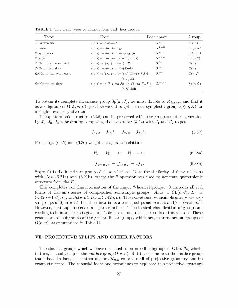
TABLE 1. The eight types of bilinear form and their groups.

Type Form Base space GroupR-symmetric ε(a,b)=ε(b,a)=a·b Rn SO(n)

R-skew ε(a,b)=−ε(b,a)=a·Jb R2n,2n Sp(n,R)

C-symmetric ε(a,b)=−ε(b,a)=a·b+i(a·K∗)b Rn,n SO(n,C)

C-skew ε(a,b)=−ε(b,a)=a·J1b+i(a·J2b) R4n,4n Sp(n,C)

C-Hermitian symmetric ε(a,b)=ε†(b,a)=a·b+i(a·Jb) R2n U(n)

C-Hermitian skew ε(a,b)=−ε(b,a)=a·Jb+i(a·b) R2n U(n)

Q-Hermitian symmetric ε(a,b)=ε†(b,a)=a·b+(a·J1b)i+(a·J2b)j R4n U(n,Q)

+(a·J3b)k

Q-Hermitian skew ε(a,b)=−ε†(b,a)=a·Jb+(a·b)i+(a·K1∗b)j R4n,4n Sk(n,Q)

+(a·K2∗b)k

To obtain its complete invariance group Sp(m, C), we must double to R4m,4m and find itas a subgroup of GL(2m, C), just like we did to get the real symplectic group Sp(m,R) fora single involutory bivector.

The quaternionic structure (6.36) can be preserved while the group structure generatedby J1, J2, J3 is broken by composing the *-operator (3.24) with J1 and J2 to get

J1∗a = J1a∗ , J2∗a = J2a

∗ . (6.37)

From Eqs. (6.35) and (6.36) we get the operator relations

J21∗ = J2

2∗ = 1 , J23 = −1 , (6.38a)

[J1∗, J2∗] = [J1, J2] = 2J3 . (6.38b)

Sp(m, C) is the invariance group of these relations. Note the similarity of these relationswith Eqs. (6.21a) and (6.21b), where the * operator was used to generate quaternionicstructure from the Ki.

This completes our characterization of the major “classical groups.” It includes all realforms of Cartan’s series of complexified semisimple groups: An−1 � SL(n, C), Bn �SO(2n+1, C), Cn � Sp(n, C), Dn � SO(2n, C). The exceptional semisimple groups are alsosubgroups of Spin(n, n), but their invariants are not just pseudoscalars and/or bivectors.16

However, that topic deserves a separate article. The classical classification of groups ac-cording to bilinear forms is given in Table 1 to summarize the results of this section. Thesegroups are all subgroups of the general linear groups, which are, in turn, are subgroups ofO(n, n), as summarized in Table II.

Vll. PROJECTIVE SPLITS AND OTHER FACTORS

The classical groups which we have discussed so far are all subgroups of GL(n,R) which,in turn, is a subgroup of the mother group O(n, n). But there is more to the mother groupthan that. In fact, the mother algebra Rn,n embraces all of projective geometry and itsgroup structure. The essential ideas and techniques to explicate this projective structure

27

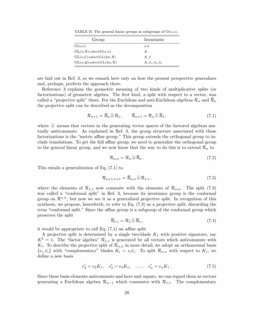
TABLE II. The general linear groups as subgroups of O(n,n).

Group InvariantsO(n,n) a·bGL(n,R)subsetO(n,n) K

GL(n,C)subsetGL(2m,R) K,J

GL(n,Q)subsetGL(4m,R) K,J1,J2,J3

are laid out in Ref. 3, so we remark here only on how the present perspective generalizesand, perhaps, perfects the approach there.

Reference 3 explains the geometric meaning of two kinds of multiplicative splits (orfactorizations) of geometric algebra. The first kind, a split with respect to a vector, wascalled a “projective split” there. For the Euclidean and anti-Euclidean algebras Rn and Rn

the projective split can be described as the decomposition

Rn+1 = Rn⊗R1, Rn+1 = Rn⊗R1 , (7.1)

where ⊗ means that vectors in the generating vector spaces of the factored algebras mu-tually anticommute. As explained in Ref. 3, the group structure associated with thesefactorizations is the “metric affine group.” This group extends the orthogonal group to in-clude translations. To get the full affine group, we need to generalize the orthogonal groupto the general linear group, and we now know that the way to do this is to extend Rn to

Rn,n = Rn⊗Rn . (7.2)

This entails a generalization of Eq. (7.1) to

Rn+1,n+1 = Rn,n⊗R1,1 , (7.3)

where the elements of R1,1 now commute with the elements of Rn,n. The split (7.3)was called a “conformal split” in Ref. 3, because its invariance group is the conformalgroup on Rn,n, but now we see it as a generalized projective split. In recognition of thissynthesis, we propose, henceforth, to refer to Eq. (7.3) as a projective split, discarding theterm “conformal split.” Since the affine group is a subgroup of the conformal group whichpreserves the split

R1,1 = R1⊗R1 , (7.4)

it would be appropriate to call Eq. (7.1) an affine split.A projective split is determined by a single two-blade K1 with positive signature, say

K2 = 1. The “factor algebra” R1,1 is generated by all vectors which anticommute withK1. To describe the projective split of Rn,n in more detail, we adopt an orthonormal basis{ei, ei} with “complementary” blades Ki = eiei. To split Rn,n with respect to K1, wedefine a new basis

e′2 = e2K1, e′3 = e3K1, . . . , e′n = enK1 . (7.5)

Since these basis elements anticommute and have unit square, we can regard them as vectorsgenerating a Euclidean algebra Rn−1 which commutes with R1,1. The complementary

28

vectors e′i = eiKi generate the corresponding anti-Euclidean algebra Rn−1 Thus we obtainan explicit projective split of Rn,n

This process can, of course, be repeated to express Rn,n as an n-fold product of com-muting R1,1 algebras. Also, similar splits can be made with respect to two-blades withnegative signature. We cannot analyze, here, the rich group structure associated with thevarious splits. Our aim is only to call attention to the possibilities.

ACKNOWLEDGMENTS

D. H. and F. S. were partially supported by a NATO Grant. C.D. is supported by aSERC studentship.

1 H. Georgi, Lie Algebras in Particle Physics (Benjamin/Cummings, Reading, 1982).2 D. Hestenes, “A Unified Language for Mathematics and Physics,” in Clifford Algebras

and their Applications in Mathematical Physics, edited by J. S. R. Chisholm and A. K.Common (Reidel, Dordrecht/Boston, 1986), pp. 1–23.

3 D. Hestenes, Acta Appl. Math. 23, 65 (1991).

4 D. Hestenes and G. Sobczyk, Clifford Algebra to Geometric Calculus, A Unified Languagefor Mathematics and Physics (Reidel, Dordrecht/Boston, 1984).

5 D. Hestenes and R. Ziegler, Acta Appl. Math. 23, 25 (1991).

6 D. Hestenes “Mathematical Viruses,” in Proceddings of the Second International Con-ference on Clifford Algebras and their Applications in Mathematical Physics, edited byA. Micali (Kluwer, Dordrecht/Boston, 1991), pp. 3–16.

7 H. Grassmann, Math. Commun. 12, 375 (1877).

8 W. Clifford, Am. J. Math. 1, 350 (1878); Mathematical Papers (1882), pp. 266–276.9 A. Crumeyrolle Orthogonal and Symplectic Clifford Algebras, (Kluwer, Dordrecht/Boston,

1991).

10E. Caianello, Combinatorics and Renormalization in Quantum Field Theory (Benjamin,Reading, MA, 1973).

11H. Weyl, The Classical Groups (Princeton University, Princeton, 1939).

12F. Sommen and N. Van Acker, Found. Phys. (in press, 1993).

13R. Delanghe, F. Sommen, and V. Soucek, Clifford Algebra and Spinor-Valued Functions(Kluwer, Dordrecht/Boston, 1992).

14A. Lasenby, C. Doran, and S. Gull, J. Math. Phys. 34, 3683 (1993).

15R. Gilmore, Lie Groups, Lie Algebras, and Some of Their Applications (Wiley, New York,1974).

16R. Ablamowicz, P. Lounesto, and J. Maks, Found. Phys. 21, 735 (1991).

29

30