LEVEL'/

C

MIL-STD-781C AND CONFIDENCE INTERVALSON MEAN TIME BETWEEN FAILURES

* AES-7905

for puJ ', !<' cl; Ii

IADMINISTRATIVE AND ENGINEERING SYSTEMS MONOGRAPH

MIL-STD-781

AND .....

CONFIDENCE INTERVALS ON MEAN _TIME BETWEEN FAILURES ,

byJ0 f--e chmee

Institute of A min on and ManagementUnion College

i FebvqoW 179 30

Y -e -.

/y

UNION COLLEGE AND UNIVERSITYINSTITUTE OF ADMINISTRATION AND MANAGEMENT

Schenectady, New York 12308

/,.

5,,

ACKNOWLEDGMENT

The author appreciates the substantial criticism and

administrative support of Professor L.A. Aroian, Union College,

and Dr. Gerald J. Hahn, General Electric Corporate Research

and Development.

Accession For

DDC & -I

By__ _-.- I ' A:' '" " :'

Ditft'. all P '/orDJI st specal

MIL-STD-781 and Confidence Intervals

SUMMARY

Various realistic examples illustrate how to obtain

confidence limits on the mean time between failures (MTBF) of

an exponential distribution from data obtained from one of the

fixed-size or sequential test plans of MIL-STD-781C.

For fixed-length tests, the methods developed by B. Epstein

and the modifications of H.L. Harter are briefly discussed. For

the sequential tests simple charts for newly developed methods

of Bryant and Schmee are given.

rI

INTRODUCTION

MIL-STD-781C "covers the requirements for reliability

qualification tests and reliability acceptance tests for

equipment that experiences a distribution of times-to-failure12

that is exponential" 1 A set of standard test plans are

provided. They are either of the fixed length or the sequen-

tial type. The performance requirement is specified in terms

of mean-time-between-failure (MTBF). Sometimes dimensions

other than time are used, e.g. cycles. Then the performance

requirement is mean-cycles-between-failures. MIL-STD-781C is

only applicable when the times to failure follow the exponential

distribution.

One of the major criticisms of a previous version of the

standard (MIL-STD-781B) was that equipment tested and accepted

by the statistical test plans often showed unacceptable time

to failure characteristics in the field. Such discrepancies

between a test method and the field may be due to statistical

and non-statistical reasons.

The test plans in MIL-STD-781B emphasized statistical

hypothesis testing of two distinct values of the MTBF, 0

versus eI . Either 0o 0was accepted and e1 rejected, or vice

versa. The accepted value was assumed to be the MTBF of

the tested equipment. However, acceptance or rejection of a

statistical hypothesis provides only limited insight into

the possible values of the MTBF. On the other hand, a

confidence interval calculated from the test data after

-- 2 -

acceptance or rejection of the equipment, provides a range

of values of statistical hypotheses (or MTBFs) which could

not be rejected on the basis of the test data. Thus a confi-

dence interval is viewed as a collection of acceptable hypo-12

theses. Confidence intervals are new in MIL-STD-781C

As a specific example, in a later section we calculate

a confidence interval on the MTBF of some electronic equipment

from 80 hours to 241 hours. This means that an hypothesis

that the MTBF is between 80 hours and 241 hours would have

been accepted, and not merely the 100 hours as stated in the

accepted hypothesis of that example. Rather than accepting

(or rejecting) a single value for the. MTBF, with a confidence

interval one can give a range of values for which a similar

decision would have been reached. This is useful to know,

because in MIL-STD-781 (and in other real world situations)

the acceptance or rejection of the statistical hypothesis

is frequently accompanied by a contractual acceptance or rejection

of equipment.

This paper presents an overview of classical methods

for confidence intervals on the MTBF of an exponential distri-

bution after completion of a life test of MIL-STD-781C. The

methods themselves are not limited to the standard, butapply

(especially after fixed-length tests) after testing assuming

an exponential distribution. The next section briefly reviews

the test p~ans of MIL-STD-781C. This is followed by sections

on confidence intervals after fixed-length tests and after

the sequential test plans.

3 --

The following are limits to the subject treated in

this paper.

* Only the statistical aspects of the test plans

are considered. Thus the important problem of

lab versus field testing is not considered

(see Yasuda 15).

* Only equipment with failure times that are either

exponential or can be transformed to the exponential

can be considered. Harter and Moore 10 looked at

the robustness of the test plans if the assumption

of exponentiality is not satisfied. In particular,

they look at Weibull failure times.

e Only confidence intervals on the MTBF after a

statistical test are discussed. This excludes the

discussion of prediction intervals or tolerance

intervals. The various types of intervals are discus-

sed in Hahn 6,7

A prediction interval is an interval which contains

a future outcome or outcomes with a specified

probability, for example,

- the time to failure of a single equipment, or

- the average time to failure of the equipment ina lot of size k, or

- all the failure times of the equipment in a lotof size k.

Prediction intervals are generally wider th3n

confidence intervals. Using a confidence inteival

when a prediction interval is required results in

-4-

a wrong, overly optimistic answer. Tolerance

intervals contain thekfailure times of a least

a specified proportion p (of the population) witf.

a stated level of confidence. Tolerance intervals

are generally also wider than confidence intervals.

Many times rather than confidence intervals,

prediction intervals or tolerance intervals are

the answer. New methods have yet to be worked out

for these types of intervals.

5-

STATISTICAL TEST PLANS

The test plans of MIL-STD-781C serve two major purposes.

In (preproduction) qualification tests they are used to ensure

that hardware reliability meets or exceeds the requirements.

Also they are used to conduct (production) acceptance tests

either through lot-by-lot sampling or for all equipment.

This section introduces the standard test plans. First,

notation and definitions are given. Then fixed-length tests

and sequential tests are briefly described and compared.

Notation:

f(t) (1/0) exp {-t/0) , t>O; the density

function of exponential failure times.

O = the true mean time between failures

(MTBF) of the exponential distribution.

Qi = lower test MTBF is an unacceptable value

of the MTBF which the standard test plans

reject with high probability.

o 0 upper test MTBF is an acceptable value of0

MTBF equal to the discrimination ratio

times 01.

d = 0o/01, the discrimination ratio; d identifies

a test plan.

E = producer's risk; the probability of

rejecting equipment(s) with a true MTBF

equal to 0 0

-6

consumer's risk, the probability of

accepting equipment(s) with the true

VMTBF equal to 01.

tAi = standardized acceptance time; equipment

is accepted, if not more then i failures

occur in t Ai01 hours.

tRi = standardized rejection time; equipment

is rejected, if at least i failures

occur at or before tRi01 hours.

= demonstrated MTBF; as defined in the

standard it is the probable range of the

true MTBF stated with a specified degree

of confidence. In this paper 0<046 is the

notation used for confidence intervals.jAA t/r = total test time t/number of failures

r; a point estimate of 0. (Note: This

is the maximum likelihood estimate for

both fixed-length and sequential test plans.)

Standard Test Plans: The standard test plans of MIL-STD-781C

provide for various combinations of producer's risks (a),

consumer's risks (a), and discrimination ratios (d). These

three parameters identify a particular test plan. The plans can

be separated into three groups:

1. Fixed-length test plans, numbered IXC through

XVIIC, and XIXC through XXIC.

2. Probability ratio sequential tests (PRST),

numhered IC through VIIIC.

-7-

3. All equipment reliability test, number XVIITC

(not covered in this paper).

Parameters of the Test Plans: The test plans in the above

first two groups are characterized by the way a test is

eventually terminated (stopping rule, truncation), and, most

important, by the three parameters a, 8, and d. The decision

risks a and 8 of the standard test plans are .1, .2, or .3;

the discrimination ratio is either 1.5, 2.0, or 3.0.

For example, to test the statistical hypotheses

H: 0 = 10 hours versus0 0

HI: 01 = 5 hours

i.e. d = 2.0 with specified risks a= a= .1, one can either

• *select the fixed-length test XIIC or the sequential test IIIC.

Table C-I of MIL-STD-781C (12, p. 64), gives a summary of

the parameters of each test plan.

The same test plan would be chosen for testing

H : 0 = 30 hours versus0 0

HI: 01 = 15 hours,

since the discrimination ratio d = 30/15 = 10/5 = 2 is the

same, assuming the same decision risks. However, the different

hypotheses make a difference, because the times to rejection

and times to acceptance are multiples of 01. Thus for acceptance

in test plan XIIC, the second hypotheses requires three times

the total ;est time of the first hypothesis, viz 15 x 18.8 hours

as opposed to 5 x 18.8 hours. In fixed-length tests the minimum

time to accept is always a multiple ofO 1 . The standard minimum

times to accept are also given in Table C-I of MIL-STD-781C.

-8-

In sequential test plans the standard acceptance times

tAi and the standard rejection times tRi must be multiplied by

01 to arrive at the actual acceptance and rejection times.

For illustration, standard acceptance and rejection times for

test plan IIIC are given in Table 1, for the other sequential

test plans they are in MIL-STD-781C (12, pp. 66-81). For

example, for test plan IIIC tA0 = 4.40, tAl = 5.79 and so on.

Thus, the first (second) hypothesis can be accepted, if

either

- no failure occurs up to tAO01 = 4.40 x 5 hours

(4.40 x 15 hours), or

- one failure occurs before tAO 1, and no failure

occurs between 4.40 x 5 hours (4.40 x 15 hours),

and

t = 5.79 x 5 hours (5.79 x 15 hours), andtAl

so on.

Nominal versus True Decision Risks: The nominal decision

risks are used to identify comparable test plans. Because

failures are measured by whole numbers, it is generally not

possible to construct a test with stated risks. The risks

actually achieved are called true decision risks. They are

very close to the nominal risks.

For example, for test plan XIIC the nominal risks are

= = 0.10, but the true risks are ax 0.096 and4

8 = 0.106. The true decision risks for the other test plans

are given in Tables II-V of MIL-STD-781C (12, pp. 12-3).

-9-

Selection of a Test Plan: One must choose between fixed-length

or sequential tests. The standard explains that a fixed-length

test must be chosen if

- the total test time is fixed in advance, or

- an estimate of the true MTBF demonstrated is

required.

Sequential tests are recommended when only an accept/reject

decision is desired.

These preceding selection criteria seem rather arbitrary

because the maximum total test time (truncation time) of a

sequential test is hardly longer than the fixed-length minimum

acceptance time. For example, the truncation time for test

plan IIIC is 20.6 01 hours, whereas the minimum acceptance

time for the equivalent fixed-length test plan XIIC is 18.8 01

hours, at worst an increase of 1.8 O hours or 8.6 percent.

However, sequential tests offer substantially earlier termina-

tion times. Test plan IIIC terminates on the average after

10.2 01 hours.

Bryant and Schmee 5 and the graphs of this paper provide

equivalent methods to those available for fixed-length tests

for estimation after a sequential test.

Sample Size and Test Length: The standard also specifies

a minimum sample size for production reliability acceptance

of at least three equipments (unless otherwise specified), or

between 10% and 20% of the lot. The sample size for a

reliability qualification test is specified in the contract.

Also, each equipment shall operate at least one-half the

average operating time of all equipment on test.

-10-

ESTIMATION AFTER A FIXED-LENGTH TEST

In estimation from life test data one must distinguish

between time censored data, when the test is terminated after

some predetermined time, and failure censored data, when the

test is terminated at the occurrence of a predetermined number

of failures. Each censoring mode requires different formulae.

In life tests, such as those of MIL-STD-781, either censoring

mode may occur: time censoring occurs, if the test is accepted;

failure censoring, if the test is rejected. However, at the

start of the test one does not know, which of the two censoring

modes will occur, so that a set of formulae or tables fitting

each outcome must be specified.

MIL-STD-781C provides methods for estimation after a

fixed-length test (but not after a sequential test). In this

section two methods for estimation after a fixed-length test are

4presented. The first, due to Epstein , is the one currently

included in MIL-STD-781C. It yields confidence intervals with

higher confidence levels than stated. The second method,

proposed by Harter 9, seems to give narrower intervals at con-

fidence levels closer to the stated ones than Epstein's method.

Because of the form of the exponential distribution both methods

do not require the actual failure times. Only the number of

failures and the total test time are accumulated. The same

holds for the methods after se;uential tests described in the

next section.

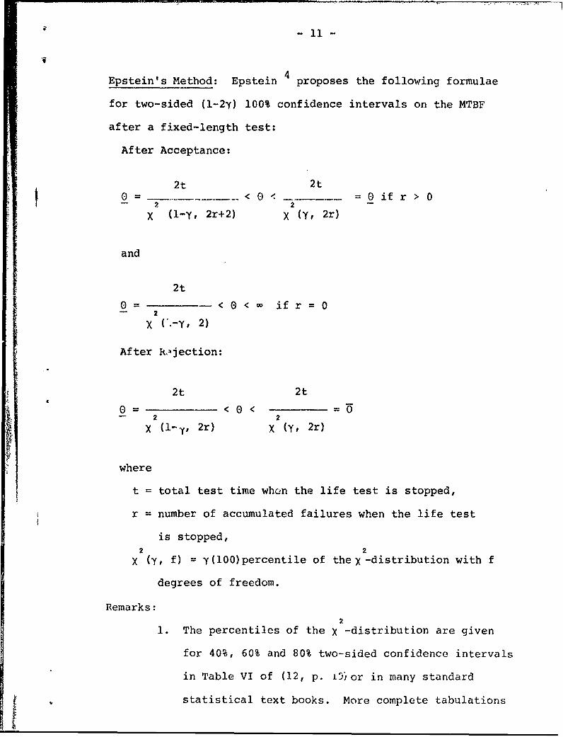
4Epstein's Method: Epstein proposes the following formulae

for two-sided (l-2y) 100% confidence intervals on the MTBF

after a fixed-length test:

After Acceptance:

2t 2t0= < E) 0 ifr > 0-- 2 2 -

X (l-y, 2r+2) X (Y, 2r)

and

2t

E)= -< 0 < if r =0- 2

X (*.-y, 2)

After RNjection:

2t 2t

0= <0< 2 2X (l-y, 2r) X (y, 2r)

where

t = total test time when the life test is stopped,

r = number of accumulated failures when the life test

is stopped,2 2X (y, f) = y(100)percentile of theX -distribution with f

degrees of freedom.

Remarks:2

1. The percentiles of the X -distribution are given

for 40%, 60% and 80% two-sided confidence intervals

in Table VI of (12, p. 5)or in many standard

statistical text books. More complete tabulations

- 12 -

8are girven in Harter

2. For (l-y) 100% one-sided confidence intervals

one uses the same formulae as for (1-2y) 100%

two-sided confidence intervals, For one-sided

lower intervals the left-hand side of the two-sided

formula is used (the upper limit is at infinity),

and for one-sided upper intervals the right-hand

side of the two-sided formula is used (the lower

limit is zero). Also note that there is no

one-sided upper confidence interval with zero

failures (r=0).

!MIL-STD-781C does not even give the formula

for r=0 for two-sided confidence intervals. The

obvious reason for this omission is that this

results in an interval which is unbounded to the

right.

3. The above formulae produce conservative confidence

intervals. This means that the true confidence

level is usually higher than stated (see Epstein

5and Fairbanks )

Example : In a fixed-length life

test of electronic equipment it is desired to accept

the equipment with probability 1-a =.9 when 0=0, = 100

hours, and to reject it with probability 1-0 =.9

when 0=0, = :v hours. Thus the discrimination ratio

d = 2.0. Test Plan XIIC is selected for this test.

-13-

From Table II of MIL-STD-781C (12, p. 12)we

find that this test plan results in acceptance,

if not more than 13 failures occur in 18.80, =

18.8 x 50 = 940 hours, and in a rejection

otherwise.

Acceptance: Suppose that only r = 7 failures

occur in 940 hours. So the test results in

acceptance of the equipment. In this case the

data are time censored. Note that the seventh

failure occurred before 940 hours.

A two-sided 80% confidence interval on the MTBF is

2 x 940 2 x 940E) < 0<

2x (.90, 16) x (.10, 14)

-1880 -79.86 < 0 <180 2.30 - 2318 1880 - 241.35 =-- 2-.5-- 418 9.6 < 7.7895

This means that the true MTBF is, with 80% confi-

dence, longer than 80 hours and shorter than 241

hours. The upper test MTBF 00 = 100 hours is

included in this interval, the lower test MTBF

01 = 50 hours is not.

Rejection: In a life test of another

lot of the above equipment, the 14-th failure

occurs after 850 hours. The test results in

rejection of the equipment and is terminated

-14-

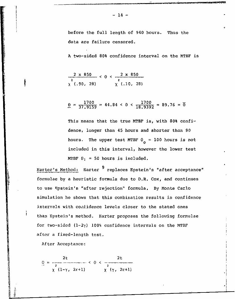
before the full length of 940 hours. Thus the

data are failure censored.

A two-sided 80% confidence interval on the MTBF is

2 x 850 2 x 850_____-<0<

2 2x (.90, 28) X (.20, 28)

_ 1700 - 44.84 < 0 < 1700 89.76-- 37.9159 18.9392

This means that the true MTBF is, with 80% confi-

dence, longer than 45 hours and shorter than 90

hours. The upper test MTBF 0 = 100 hours is noto

included in this interval, however the lower test

MTBF 01 = 50 hours is included.

9Harter's Method: Harter replaces Epstein's "after acceptance"

formulae by a heuristic formula due to D.R. Cox, and continues

to use Epstein's "after rejection" formula, By Monte Carlo

simulation he shows that this combination results in confidence

intervals with confidence levels closer to the stated ones

than Epstein's method. Harter proposes the following formulae

for two-sided (1-2y) 100% confidence intervals on the MTBF

after a fixed-length test.

After Acceptance:

2t 2t0-< 0<- 2 2

X (1-y, 2r+l) X (y, 2r+l)

S- 15 -

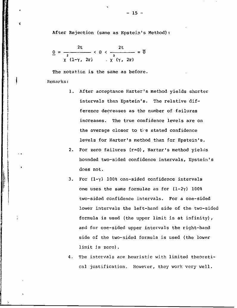
After Rejection (same as Epstein's Method):

2t 2t0=- << =

- 2 2X (l-y, 2r) X (y, 2r)

The notation is the same as before.

IRemarks:1. After acceptance Harter's method yields shorter

intervals than Epstein's. The relative dif-

ference decreases as the number of failures

increases. The true confidence levels are on

the average closer to t'-e stated confidence

levels for Harter's method than for Epstein's.

2. For zero failures (r=0), Harter's method yields

bounded two-sided confidence intervals, Epstein's

does not.

3. For (l-y) 100% one-sided confidence intervals

one uses the same formulae as for (l-2y) 100%

two-sided confidence intervals. For a one-sided

lower intervals the left-hand side of the two-sided

formula is used (the upper limit is at infinity),

and for one-sided upper intervals the right-hand

side of the two-sided formula is used (the lower

limit is zero).

4. The intervals are heuristic with limited theoreti-

cal justification. However, they work very well.

-16-

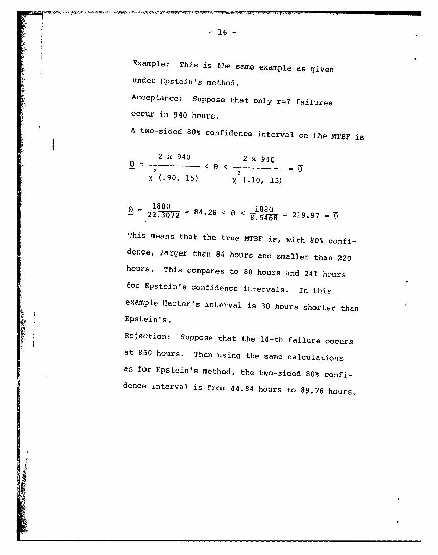
Example: This is the same example as given

under Epstein's method.

Acceptance: Suppose that only r=7 failures

occur in 940 hours.A two-sided 80% confidence interval on the MTBF is

2 x 940 2 x 940o = ------ < 0) < _-- = 'd

X (.90, 15) X (.10, 15)

1880 1880

223072 = 84.28 < 0 < 8.5468 219.97 =

This means that the true MTBF is, with 80% confi-dence, larger than 84 hours and smaller than 220

hours. This compares to 80 hours and 241 hoursfor Epstein's confidence intervals. In this

example Harter's interval is 30 hours shorter than

Epstein's.

Rejection: Suppose that the 14-th failure occursat 850 hours. Then using the same calculations

as for Epstein's method, the two-sided 80% confi-dence interval is from 44.84 hours to 89.76 hours.

-17-

ESTIMATION AFTER A SEQUENTIAL TEST

This section presents charts for obtaining confidence

intervals on the exponential MTBF after a sequential test.3

They are based on the work of Bryant and Schmee .Previously

various attempts at sequential estimation have been made bySumerlin 14 Aroian and Oksoy and Luetjen They are

3briefly discussed in Bryant and Schmee

The use of the charts given here is similar to the

formulae for estimation after a fixed-length test. There are

separate charts for tests resulting in acceptance and those

resulting in rejection. As with Epstein's method the associated

overall confidence level is conservative. This means that the

intervals hold for a confidence level at least as high as stated.

The charts are more convenient to use than the tables

3given in Bryant and Schmee . Particularly when a test ends

in rejection, the tables have to be interpolated but the charts

do not. A disadvantage of the use of the charts is the limited

accuracy with which the multipliers can be read.

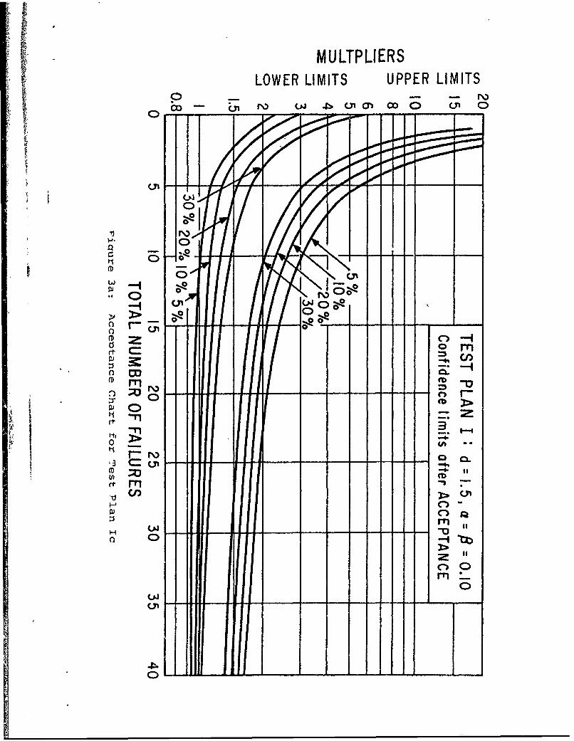
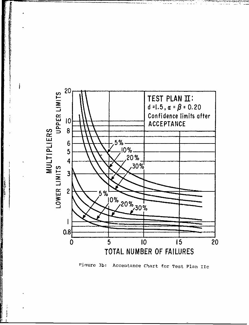
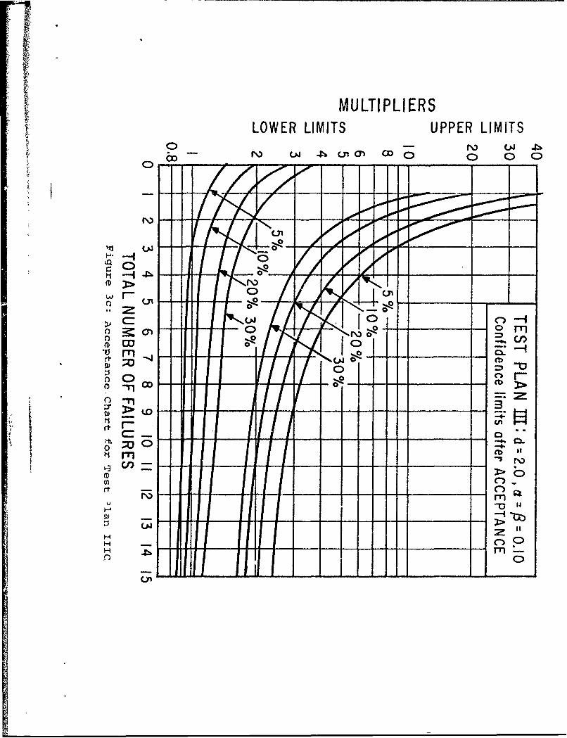
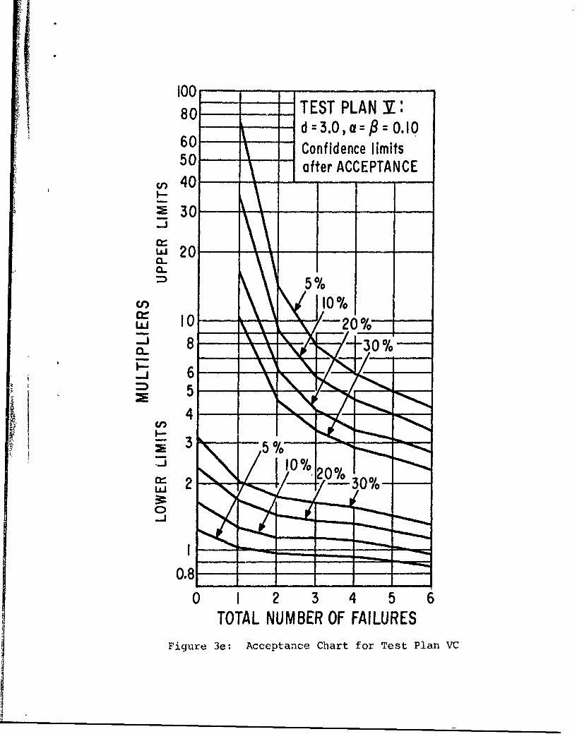
For each test plan there are two charts, one for accept

decisions and one for reject decisions. For test plans VIC and

VIIIC after acceptance numerical values are given instead of the

charts (Table 2 ). There are very few acceptance points and

so charts did not seem advisable.

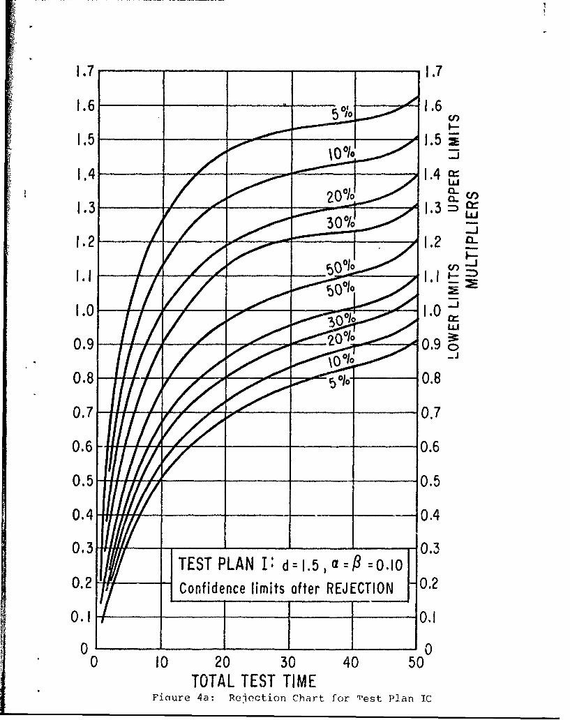
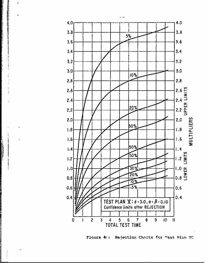
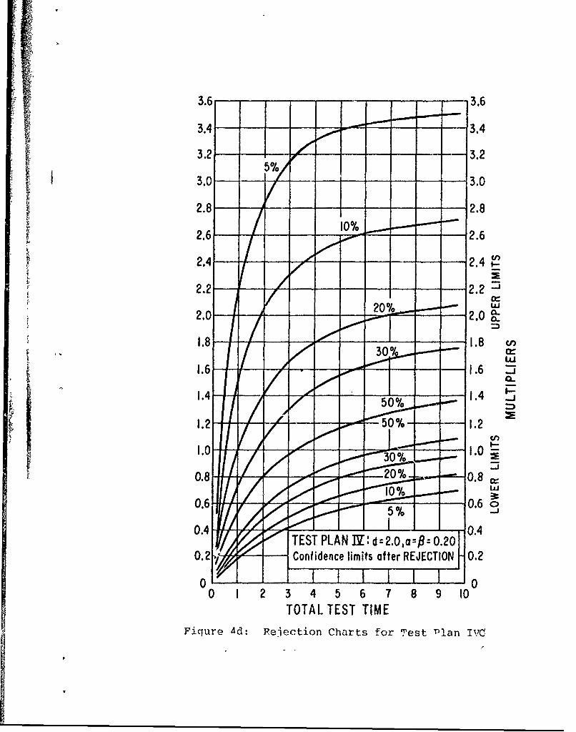
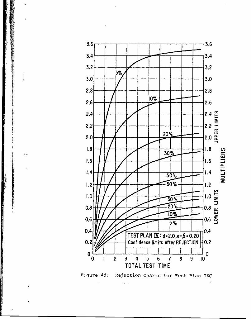
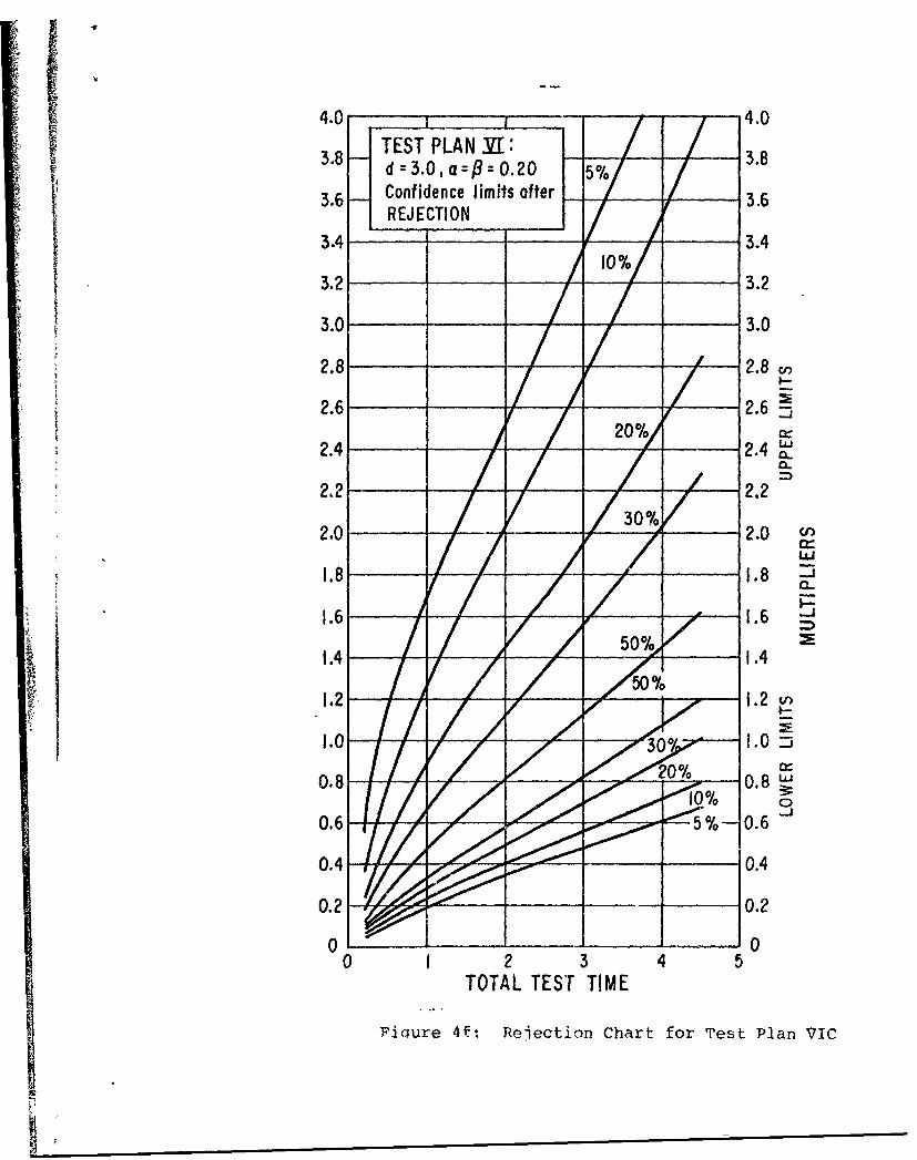
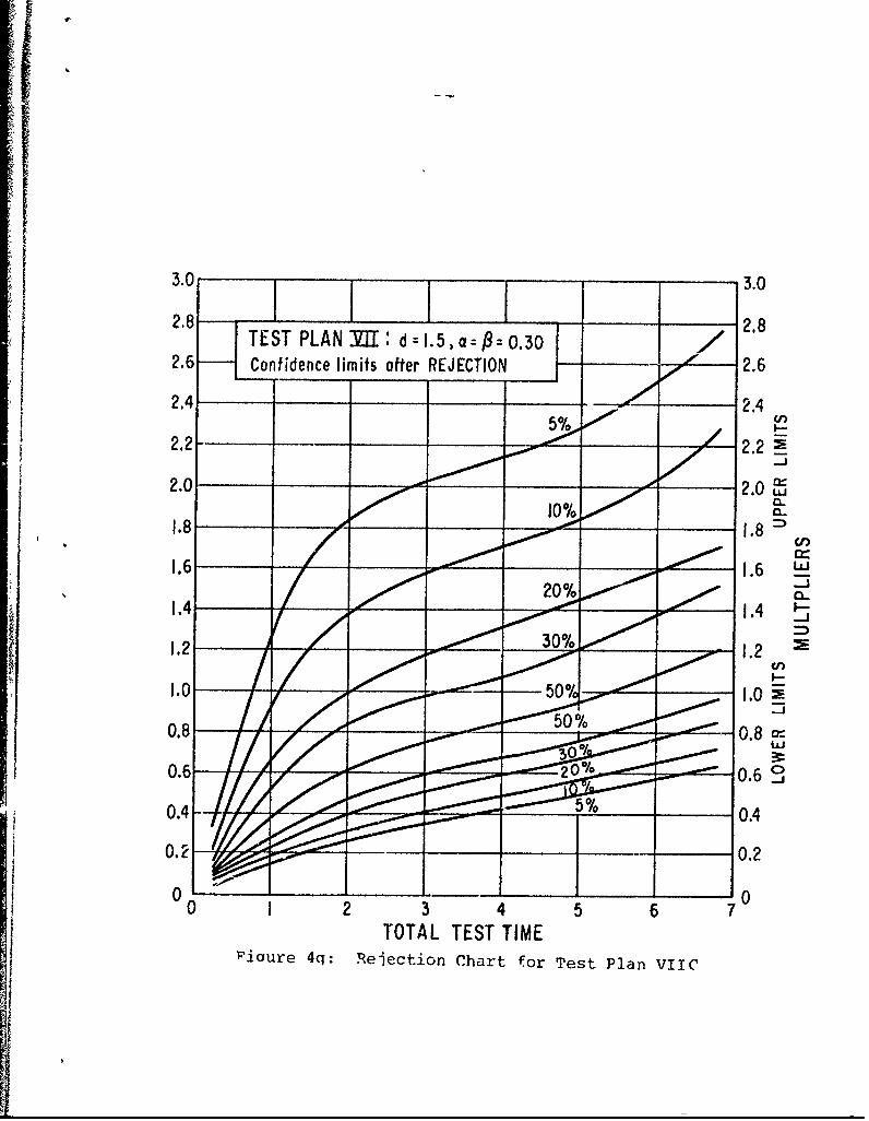
The charts contain lower and upper lines marked 5%, 10%,

20%, 30%. Rejection charts also contain a 50% line. Multipliers

from the 10% lines can be used to find 90% one-sided (upper or

-18-

lower) confidence intervals, or two-sided 80% confidence

intervals. Similarly one uses the 5% (20%)(30%) lower or

upper lines to construct 95% (80%)(70%) one-sided lower or

upper confidence intervals, or 90% (60%)(40%) two-sided confi-

dence intervals on the MTBF.

Examplefor Confidence Intervals after Acceptance:

In this example a sequential test similar to the

fied-length test example of the previous section is described,

E]ectronic equipment is tested with the following specs:

0 = 100 hours, 01= 50 hours, x = = 0.10, and d = 2.0. Test

Plan IIIC is used.

In this test six relevant failures occurred after the

following accumulated total test times: 56.3, 137.9, 201.3,

388.7, 501.4, 510.8 hours. The test results in acceptance after

636 hours, since during that time only six relevant failures

occurred. The test could not have resulted in acceptance with

five failures, since the sixth failure occurred before

tA50 = 11.34 x 50 = 567 hours, nor could it have been accepted

earlier, nor rejected.

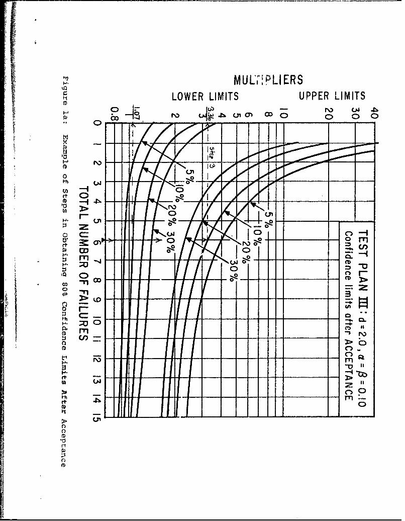
To calculate 80% two-sided confidence limits one proceeds

as follows (see Figure la):

1. Go to the acceptance chart for Test Plan IIIC

and mark the number of failures (six) on the

horizontal axis.

2. Go up the vertical line and mark the points

of intersection with the 10% lower and 10%

upper lines.

-19-

3. Draw horizontal lines through the points of

intersections, and mark the point of inter-

section of the horizontal line with the verti-cal axis.

4. Read off the lower and upper multipliers

from the vertical axis; the lower multiplier

is 1.07, the upper multiplier is 3.36.

5. Multiply the lower (upper) multiplier by

01 = 50 to obtain the lower limit 0 (upper

limit U).

Thus the 80% two-sided confidence interval on 0 is

0 = 1.07 x 50 = 53.50 < 0 < 3.36 x 50 = 168.0 =

This means that with 80% confidence the true MTBF

is longer than 54 hours and shorter than 168 hours.

The lower test MTBF 01 = 50 hours is not included

in this interval, but the upper test MTBF 00 = 100 hours

is included.

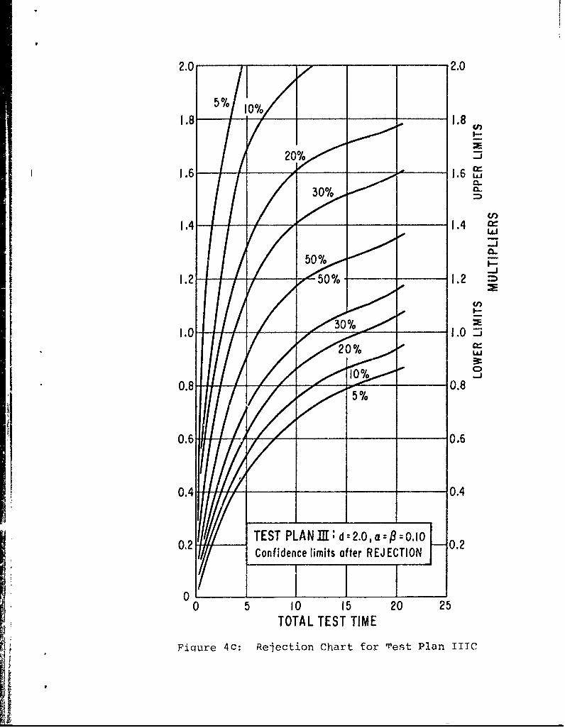
Example for Confidence Intervals after Rejection:

As before we test equipment with Test Plan IIIC, and

assume 0 = 100 hours, 01 = 50 hours, a = 8 = 0.10, and0

d = 2.0.

The actual relevant failure times are now recorded as

10.2, 12.7, 37.7, 108.3, 187.4, 267.2, 302.6 hours. The test

results in a rejection after 302.6 hours, since the seventh

failure occurs before the critical failure time

tR7 x 01 = 6.24 x 50 = 312 hours. The test could not have

been rejected after 267.2 hours with six failures since the

MUW:" PLIERSLOWER LIMITS UPPER LIMITS

0

cj -

rt 0

~Q 00

C=

rn

rt*1

CrCL

rtn

a,0

- 20 -

critical failure time tR6 x 0, = 4.86 x 50 = 243 hours is

smaller than the actual failure time; nor could it have been

rejected at any of the previous failures; nor could it have been

accepted.

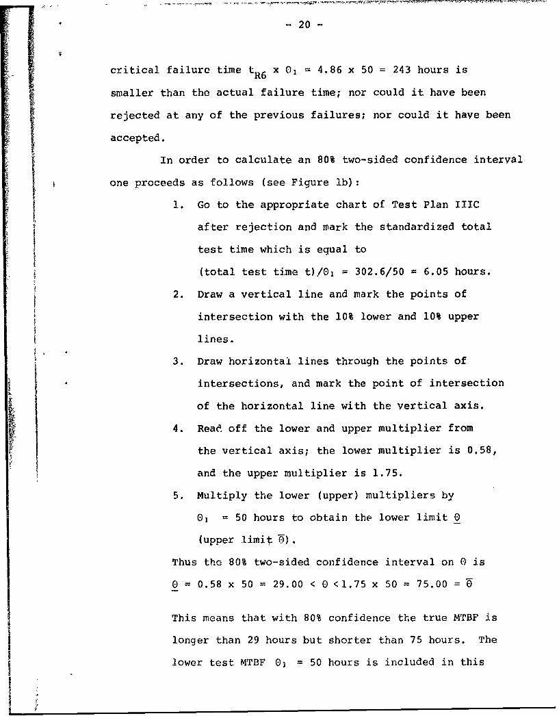
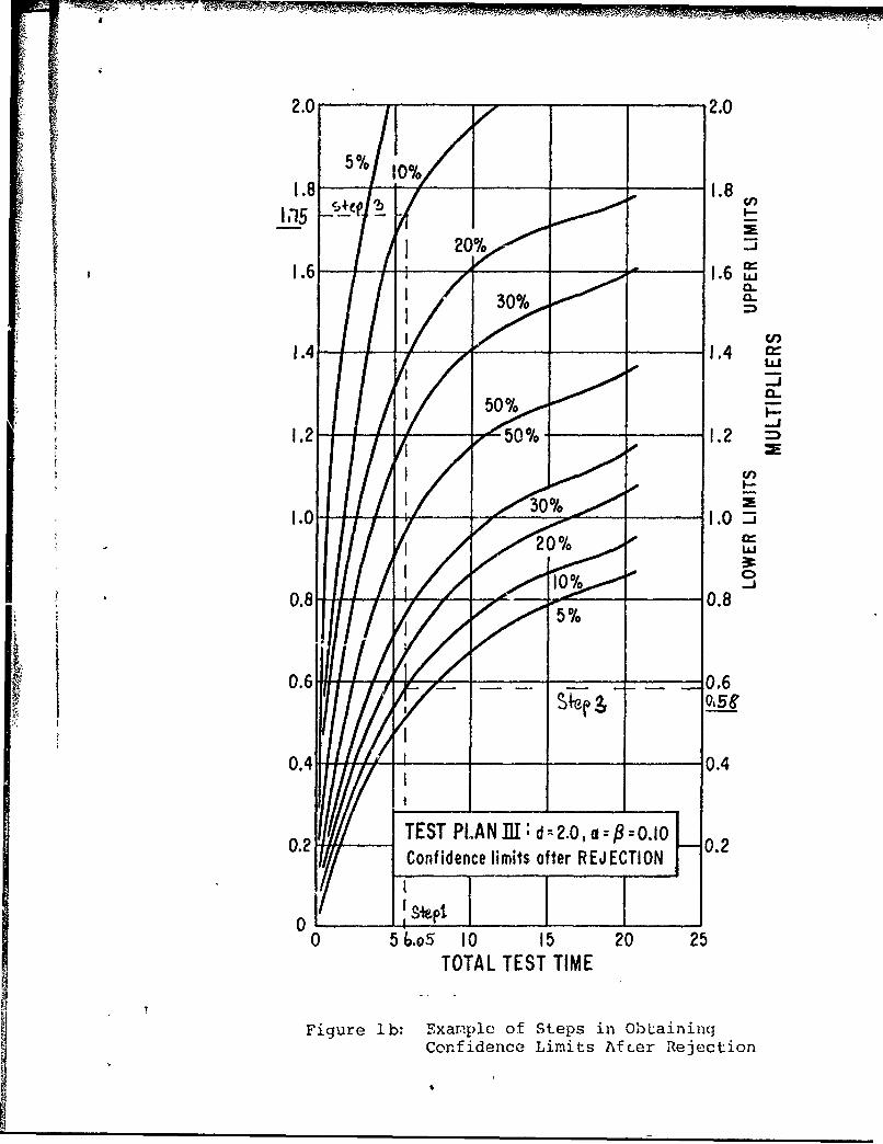
In order to calculate an 80% two-sided confidence interval

one proceeds as follows (see Figure ib):

1. Go to the appropriate chart of Test Plan IIIC

after rejection and mark the standardized total

test time which is equal to

(total test time t)/0 1 = 302.6/50 = 6.05 hours.

2. Draw a vertical line and mark the points of

intersection with the 10% lower and 10% upper

lines.

3. Draw horizontal lines through the points of

intersections, and mark the point of intersection

of the horizontal line with the vertical axis.

4. Read off the lower and upper multiplier from

the vertical axis; the lower multiplier is 0.58,

;and the upper multiplier is 1.75.

5. Multiply the lower (upper) multipliers by

01 = 50 hours to obtain the lower limit 0

(upper limit ).

Thus the 80% two-sided confidence interval on 0 is

0 = 0.58 x 50 = 29.00 < 0 <1.75 x 50 = 75.00 = 0

This means that with 80% confidence the true MTBF is

longer than 29 hours but shorter than 75 hours, The

lower test MTBF 01 = 50 hours is included in this

I

2.0 5/1100/2.0

1.8 -1 .8

1.6 1.6

.430% =

1.4 -11.42 C

1.2 j 01.

1.0 31.01.0 0__0 _

10%

0.80.8 -

0.4 0.4

TEST PLAN]JX d=2.0, a =0.100.2 Confidence limits otter REJECTION

0L... Sp ______I__

0 56-05 10 15 20 25TOTAL TEST TIME

Figure ib: Example of steps in ObLaininqConfidence Limits Aft~er 'Rejection

-21-

interval, but the upper test MTBF 0 100 hours

is not.

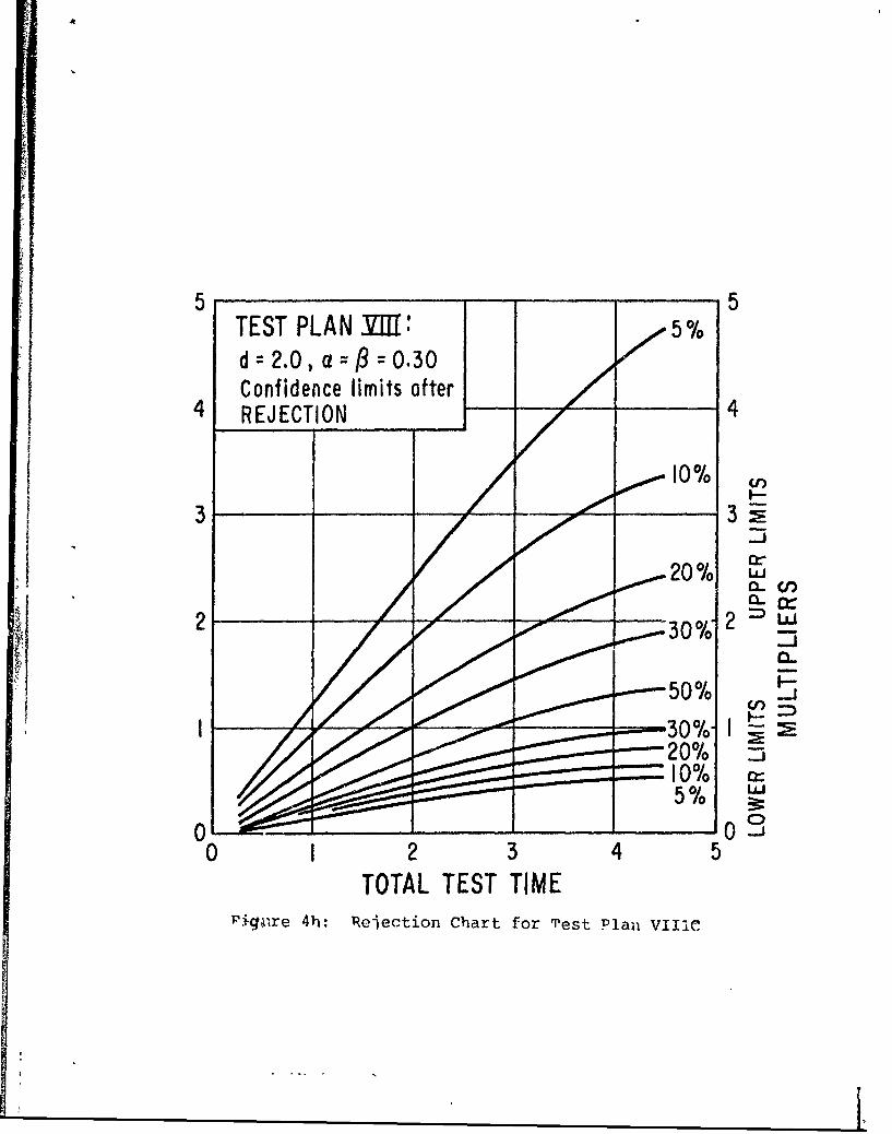
Other Charts and Tables

The charts cover all standard test plans of MIL-STD-781C.The acceptance charts are Figure 3, a-f. The rejection charts areFigure 4, a-h. Acceptance multipliers for Test Plans VIC and

VIIIC are given in Table 2.

In calculating confidence intervals for these charts onefollows the same steps as outlined in the previous example forTest Plan IIIC.

I

22-

CONCLUDING REMARKS

1. Choice of the Confidence Level: Certain confidence levels

seem to be more appropriate than others. The example used

for confidence intervals after acceptance in test plan

IIIC illustrates this. The test was terminated after not

more than six failures occurred in 636 hours. The 80%

two-sided confidence interval was calculated from 54 to

168 hours. Suppose one would have chosen the 90% confidence

level instead. Following the steps as outlined in that

section, the multipliers are 0.94 and 4.0 resulting in a

90% two-sided confidence interval from 47 hours to 200 hours.

This interval includes both the lower test MTBF 01 and the

upper test MTBF 00.0

This example shows that a confidence level above

(l-2a) 100% for two-sided intervals and above (1-a) 100%

for one-sided intervals (assuming c=O ) may result in inter-

vals which include both 0 and 01.0

2. Length of Confidence Intervals: As mentioned before, Harter's

method usually results in shorter confidence intervals after

acceptance than Epstein's.

A similar comparison between intervals after a fixed-length

test and a sequential test is more difficult, because the

stopping rules are different. Equal number of failures in

the same length of time usually do not occur.

d

-23 j

Using an example from before shows this. A fixed-length

test resulted in acceptance with seven failures after 940

hours. The 80% two-sided confidence interval on the MTBF

is from 80 to 241 hours for Epstei.t's method, 84 to 220

hours for Harter's method. A sequential test with seven

failures would have been terminated after only 705 hours

with an 80% two-sided confidence interval from 53 to 152

hours. The interval after 705 hours of total sequential

test time is only 99 hours long as opposed to 161 (or 136)

hours after 940 hours of total fixed-size test time.

However, the lower limit of the sequential interval is

much closer to 01 than the lower fixed-length limit. This

is so, because the sequential test accepts (or rejects) as

soon as possible. In other words, it accepts (or rejects)

as soon as a (1-2a) 100% two-sided confidence interval is

narrow enough not to cover both 0 and 01.0

REFERENCES

1. AROIAN, L.A. Application of the direct method in

sequential analysis. Technometrics, 18, August

1976, pp 301-306.

2. AROIAN, L.A. and OKSOY, D. Estimation, confidence

intervals, and incentive plans for sequential three-way

decision procedures. 1972 NATO Conference Proceedings

on Reliability Testing and Evaluation, VI-D-l to FI-D-13.

3. BRYANT, C. and SCHMEE, J. Confidence Limits on MTBF

for Sequential Test Plans of MIL-STD-781. Technometrics,

21, February 1979, to appear.

4. EPSTEIN, B. Estimation from life test data. Technometrics,

2, November 1960, pp 447-454.

5. FAIRBANKS, V.B. Two Sided Confidence Intervals for an

Exponential Parameter. Technical Report No. 73, Dept.

of Statistics, University of Missouri-Columbia, January

1978.

6. HAHN, G.J. Statistical Intervals for a Normal Population,

Part I. Journal of Quality Technology, 2, July 1970

7. HAHN, G.J. Statistical Intervals for a Normal Population,

Part II. Journal of Quality Technology, 2, October 1970,

pp 195-206.

8. HARTER, H.L. New tables of the incomplete gamma function

ratio and of percentage points of the chi-square ard

beta distribution. U.S. Government Printing Office,

Washington, D.C., 1964.

9. HARTER, H.L. MTBF Confidence Rounds Based on MIL-STD-781C

Fixed-Length Vest Results. Journal of Quality Technology,

10, October 1978, pp 164-169.

I10. HARTER, H.L. and MOORE, A.H. An evaluation of exp~nentiai

and Weibull test plqns. IEEE Transactions on Reliability,

R-25, June 1976, pp 100-104.

11. LUETJEN, P. Tables of parametric confidence limits from

hypothesis test data. NAVSEC Report 6112-75-1, Naval

Ship Engineering Center, Hyattsville, Maryland, 1974.

12. MIL-STD 781C, Militar Standard Reliability Qualification

on Production Acceptance Tests% Exponential Distribution,

Washington, D.C., 1977.

13. NEATHAMMER, R.D, PABST, W.R, and WIGGINTON, C.G.

MIL-STO 781B, reliability tests: exponential distribu-

tion. J. Quality Teohnology, 1, January 1965, pp 58-67.

14. SUMERLIN, W.T. Confidence calculations for MIL-STD 781.

1972 Annual Reliability and MaintainabilityS

IEEE Catalog Number 72CH0577-B, January 1972, pp 205-212.

15. YASUDA, J. Correlation Between Laboratory Test and Field

Part Failure Rates. IEEE Transactions on Reliability,

R-26, June 1977, pp. 82-84.

PP

I

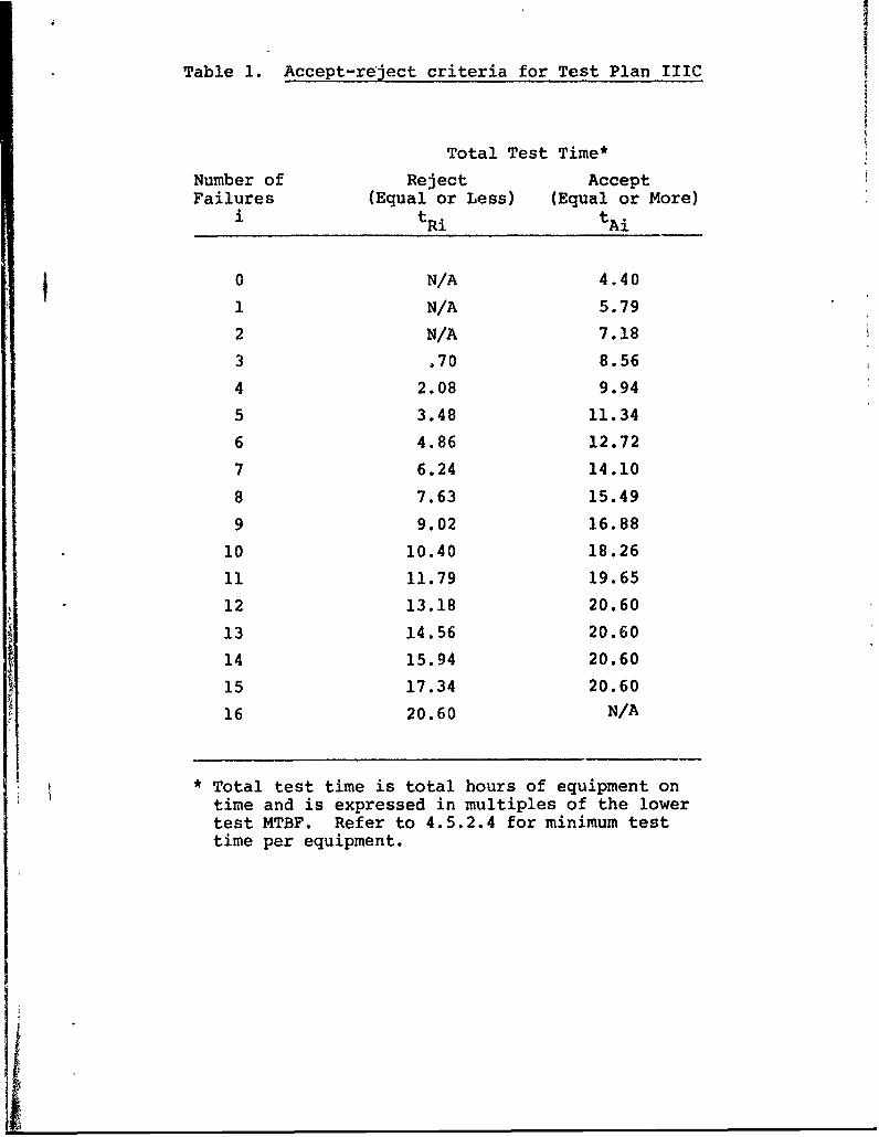
Table 1. Accept-reject criteria for Test Plan IIIC

Total Test Time*

Number of Reject AcceptFailures (Equal or Less) (Equal or More)

i tRi tAi

j 0 N/A 4.40

1 N/A 5.79

2 N/A 7.18

3 .70 8.56

4 2.08 9.94

5 3.48 11.34

6 4.86 12.72

7 6.24 14.10

8 7.63 15.49

9 9.02 16.88

10 10.40 18.26

11 11.79 19.65

12 13.18 20.60

13 14.56 20.60

14 15.94 20.60

15 17.34 20.60

16 20.60 N/A

* Total test time is total hours of equipment on

time and is expressed in multiples of the lowertest MTBF. Refer to 4.5.2.4 for minimum testtime per equipment.

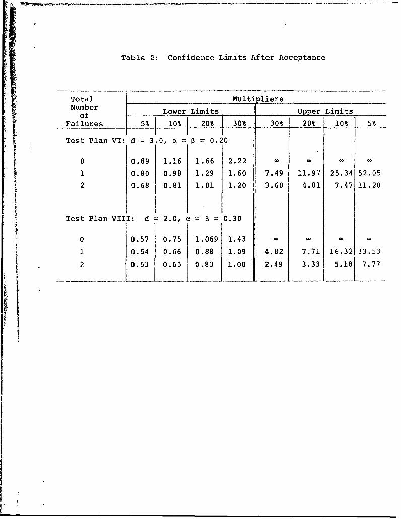
ITable 2: Confidence Limits After Acceptance

Total MultipliersNumber Lower Limits Upper Limitsof

Failures 5% 10% 20% 30% 30% 20% 10% 5%

Test Plan VI: d = 3.0, a = 8 = 0.20

0 0.89 1.16 1.66 2.22 O 0 O

1 0.80 0.98 1.29 1.60 7.49 11.97 25.34 52.05

2 0.68 0.81 1.01 1.20 3.60 4.81 7.47 11.20

Test Plan VIII: d 2.0, a = = 0.30

0 0.57 0.75 1.069 1.43 G O 0

1 0.54 0.66 0.88 1.09 4.82 7.71 16.32 33.53

2 0.53 0.65 0.83 1.00 2.49 3.33 5.18 7.77

MULIPLIERSLOWER LIMITS UPPER LIMITS

000

o00000 00o

o 00

-- 0

0 r- 1--0 0-

00rtiT

Cl))

o rl- -0

0 0~

rI,

00r-o ___

IA

TEST PLAN ]I

d =1.5, a 0:,20____ ____ Confidence limits after

~lO _____ACCE PTACECn 8

L 5%

03

-5%

0 5 10 15 20TOTAL NUMBER OF FAILURES

Picqure 3b: Acceotance Chart for Test Plan Iho

MULTI PLIERSLOWER LIMITS UPPER LIMITS

co o*- 00 C

Fi-. -H of

c C

0l

(DW

Iol-4

r1,4,-C

" mU)-3

Hn

_ _ T I0 0~

60--50-- TEST PLANE:~40 -d=2.0, a=/30.20

Confidence limits30-3- after ACCEPTANCE

~20

0-

0= 100%

8 5%

0~1054

3

w

08

0 1 2 3 4 5 6 7TOTAL NUMBER OF FAILURES

Fiqure 3d: Acceptance Charts for T.P. IVC

100 --

80--- . TEST PLAN V:- -- d=3.0,a= 0.10

60 Confidence limits40- \ after ACCEPTANCE

_ 30-

' w 20 . .

0-

5%cr 1 10%1w 10-0

a- 8 30%

I-"

5

0 1 2 3 4 5 6TOTAL NUMBER OF FAILURES

Figure 3e: Acceptance Chart for Test Plan VC

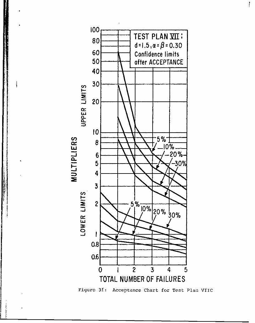
100-TEST PLAN MEE

80d=1.5, a= P=0.3060 Confidence limits50 - after ACCEPTANCE40

n0~

a-

10.-

W 5%-5-10%

4

3

2 -5

0 2 I0%00o/

0 __%

0 1 2 3 4 5TOTAL NUMBER OF FAILURES

Figure 3f: Acceptance Chart for Test Plan~ VIIC

1.7 1.7

1.6 - 1-01.6

1.5 1.5 ':

0/44w

1.3 1.31.00 1.

I L CL

0.7

0.3 - 0.3

00 0 1

30,400500.8- ~ TTA ES TIME w 00 .

0.7 r a:0 Reeto Chr0fr.7tPln

4.0 -- - - - - 4.0

3.4 ----- 34

3.2-------------3.2

2. - - - - - - -- - - - - .0

10%~

Cl)

0.4 0.4 -

0~~2 % 2 w 0ITOTA TEST TIME

Fic00r 4e eetonCet~~t ~ PmV

2. .

2.0 2.0

O%1.8 0 .

1.6 1I.6 'rQ-

1.4 ~1.4 I

-

1.2Vj v1.2

loo

20%

0. 0/ 0.8

0.6 0.6

0.4 0.4

0.2 TEST PLAN Ml1 d 2.0, a /0.10 0.0.2 Confidence limits after REJECTION

0 5 10 15 20 25

TOTAL TEST TIME

Plqure 4c: Rejection Chart for rest Plan IIIC

3.6 - - - - - - 3.6

2.8- - 2.8

2.6 110%- 2.6

2.44

2.2 L2.2 -

2.0 2.0 2L

Z. e1.8l 10

1.61 1.6 :3

1. 01.4

cr)

1.01.0

0.8 et0-1 2!%0.

0.6

0. EST PLAN ]Y: d 2.O~ acz:$ 0.20 0.0.2,Confidence limits otter REJECTION0.

0 00 1 2 3 4 5 6 7 8 9 10

TOTAL TEST TIMEFiqure 4d: Rejection Charts for Test Plan IVC.

3.6 -- 3.6

3.4-- -- 3.4

3.0- 3.0

2.8 2.8

2.610 2.6

2.4 2.4 ~

2.2 L 2.2 -

20%j

2.0- 2.0 cl

1.8 1.8 c

--6 1.6 :3

1.2 00/ - 1.2

1.0c10 1.0

0.80 0

0.6 060

0.4 TEST PLAN ID :d=2.0,a=R:0.2010.2.1Contidence limits after REJECTION 0.2

0 00 1 2 3 4 5 6 7 8 9 10

TOTAL TEST TIME

Fiqure 4d: Rejection Charts for Test Plan IVC

4.0 __ _ _ _ _ _ _ _ _4.0

3.8 TEST PLAN X~Y: 3.8d =3.0, a= fl 0.20 1013.6- Confidence limits otter 3.6

34 REJECTION __3.

3.2 10// - 3.2

3.0 3.0

2.82.

2.62.

2.42.

2.2 .2.2

2.0 2.0

L

1.6 1.6 ~

K1.4 * 1.4

1.2 1.2v

1.0-3103

0.8 1002K0.8 cui

0.6 5

0.4 - .

0.2 - .

0 .00 I2 3 4 5

TOTAL TEST TIME

Piaure 4f: Rejection Chart for Test Plan 'VC

3.0 3.02.82.

TEST PLAN MIi d 1.5,a~3 0.302.6 Confidence limits after REJECTION -2.6

2.4 2.4

2.2 2.2

2.0 2.0 'U'

1'1.8 1.81.61.

20 %1.4 - 1.4

1.2 1.2

1.0__ ___ _ I0.4 0.4

0.2 -.

00 1 2 3 4 5 6 7TOTAL TEST TIME

a ~Viaure 4q: Rejection Chart for Test Plan VIic

5 5TEST PLAN _W: 5 %d =2.0, a = p =O.30

Confidence limits after '04 REJECTION4

10%

3

20% Uj0CI)

50% -

10% M5% u

01 C

0 1 2 3 4 5TOTAL TEST TIME

~igure 4h: Rejection Chart for Test Plan vine.

UnclassifiedSECUIM7Y CLASSIVICATIO4 Or THIS PAGE ,10h flnot& Frreretd)

REPORT DOCUMENTATION PAGE READ INSTRUCTIONSBEFORE COSPIXETING FORM

I. RE'ORT NUMBER 2. GOVT ACCESSION NO, 3. RECIPIENTS CATALOG NUUMBR

i=AES-7905 -

. TITLE(nd S -btitle) S. TYPE OF REPORT &PERIOD COVEREo

MIL-STD-781C and Confidence Intervals Technical Report--on Mean Time Between Failures 6/1/78-3/1/79

6. PERFORMING ORG. REPORT NUMBER

7. ATOR() .. .... CONTRACT OR GRANT NUMBER(u)

Josef Schmee N00014-77-C-0438

3. PERFORMING ORGANIZATION NAME AND ADDRESS 10. PROGRAM ELEMENT. PROJECT. TASKInstitute of Administration and Manage- AREAA ORKUNITNUMUERSment, Union CollegeSchenectady, NY 12308

,,. CONTROLLING OFFICE NAME AND ADORESS 12. REPORT DATEOffice of Naval Research Feb. 28, 1979Department of Navy I. NUMmER Of PAGESArlington, VA 25 + 14 charts & 2 table

I4. MONITORING AGENCY NAME A ADORESS( I dillent tor Controllin Office) IS. SECURITY CLASS. (01 this roPo)

Unclassified

13a. OECL ASSIFICATION/ DOWNGRADINGSCHEDULE

16. DISTRIBUTION STATEMENT (of $hl Report)

Approved for public release; distribution unlimited.

17. DISTRIBUTION STATEMENT ( .' os .bac .ne,..din Black 20. " di.,ei ham R.p.,t)

,|. SUPPLEMENTARY NOTES

I. KEY WORDS (Continue on #*veto* ##de It noceeeq and Identify by block nmmbo,)

Exponential distribution, confidence limits, sequential tests,fixed-length test, MTBF.

'0, ABSTRACT (Continue on #over@* side is ciscey andl. dnity by block bnmb ,Vari ous realisticexamples illustrate how to obtain confidence limits on the meantime between failures (MTBF) of an exponential distribution fromdata obtained from one of the fixed-size or sequential test plansof MIL-STD-871C. For fixed-length tests, the methods developedby B. Epstein and the modifications of H.L. Harter are brieflydiscussed. For the sequential tests simple charts for newlydeveloped methods of Bryant and Schmee are given.

DD Io. 1473 EOrTIOI F I NOV 61 IS OBSOLETE

DD , oN$/N UnclassifiedISCURITY CLASSIFICATION OF TNS PAGE (When Doit Enlered)

Unclassified.Li..SCTY CLASSIFICATION OF THIS PAGE(Who 0 Dat. Ef.d,

UnclassifiedSECURITY CLASSIFICATION OF THIS PAGI(Than Dit& Ent*red)