lectures on k¨ahler manifolds - max planck...
TRANSCRIPT
ESI Lectures in Mathematics and Physics
Werner Ballmann
Lectures on Kahler Manifolds

To my wife Helga
Preface
These are notes of lectures on Kahler manifolds which I taught at the Univer-sity of Bonn and, in reduced form, at the Erwin-Schrodinger Institute in Vi-enna. Besides giving a thorough introduction into Kahler geometry, my mainaims were cohomology of Kahler manifolds, formality of Kahler manifolds af-ter [DGMS], Calabi conjecture and some of its consequences, Gromov’s Kahlerhyperbolicity [Gr], and the Kodaira embedding theorem.
Let M be a complex manifold. A Riemannian metric on M is called Her-mitian if it is compatible with the complex structure J of M ,
〈JX, JY 〉 = 〈X,Y 〉.
Then the associated differential two-form ω defined by
ω(X,Y ) = 〈JX, Y 〉
is called the Kahler form. It turns out that ω is closed if and only if J isparallel. Then M is called a Kahler manifold and the metric on M a Kahlermetric. Kahler manifolds are modelled on complex Euclidean space. Exceptfor the latter, the main example is complex projective space endowed with theFubini–Study metric.
Let N be a complex submanifold of a Kahler manifold M . Since the re-striction of the Riemannian metric of M to N is Hermitian and its Kahlerform is the restriction of the Kahler form of M to N , N together with theinduced Riemannian metric is a Kahler manifold as well. In particular, smoothcomplex projective varieties together with the Riemannian metric induced bythe Fubini–Study metric are Kahlerian. This explains the close connection ofKahler geometry with complex algebraic geometry.
I concentrate on the differential geometric side of Kahler geometry, exceptfor a few remarks I do not say much about complex analysis and complexalgebraic geometry. The contents of the notes is quite clear from the tablebelow. Nevertheless, a few words seem to be in order. These concern mainlythe prerequisites. I assume that the reader is familiar with basic conceptsfrom differential geometry like vector bundles and connections, Riemannianand Hermitian metrics, curvature and holonomy. In analysis I assume thebasic facts from the theory of elliptic partial differential operators, in particularregularity and Hodge theory. Good references for this are for example [LM,Section III.5] and [Wa, Chapter 6]. In Chapter 8, I discuss Gromov’s Kahlerhyperbolic spaces. Following the arguments in [Gr], the proof of the main resultof this chapter is based on a somewhat generalized version of Atiyah’s L2-indextheorem; for the version needed here, the best reference seems to be Chapter13 in [Ro]. In Chapter 7, I discuss the proof of the Calabi conjecture. Withoutfurther reference I use Holder spaces and Sobolev embedding theorems. This isstandard material, and many textbooks on analysis provide these prerequisites.
iv Preface
In addition, I need a result from the regularity theory of non-linear partialdifferential equations. For this, I refer to the lecture notes by Kazdan [Ka2]where the reader finds the necessary statements together with precise referencesfor their proofs. I use some basic sheaf theory in the proof of the Kodairaembedding theorem in Chapter 9. What I need is again standard and can befound, for example, in [Hir, Section 1.2] or [Wa, Chapter 5]. For the convenienceof the reader, I include appendices on characteristic classes, symmetric spaces,and differential operators.
The reader may miss historical comments. Although I spent quite sometime on preparing my lectures and writing these notes, my ideas about thedevelopment of the field are still too vague for an adequate historical discussion.
Acknowledgments. I would like to acknowledge the hospitality of the Max-Planck-Institut fur Mathematik in Bonn, the Erwin-Schrodinger-Institute inVienna, and the Forschungsinstitut fur Mathematik at the ETH in Zurich,who provided me with the opportunity to work undisturbed and undistractedon these lecture notes and other mathematical projects. I am grateful toDmitri Anosov, Marc Burger, Thomas Delzant, Beno Eckmann, Stefan Hilde-brandt, Friedrich Hirzebruch, Ursula Hamenstadt, Daniel Huybrechts, Her-mann Karcher, Jerry Kazdan, Ingo Lieb, Matthias Lesch, Werner Muller,Joachim Schwermer, Gregor Weingart, and two anonymous referees for veryhelpful discussions and remarks about various topics of these notes. I wouldlike to thank Anna Pratoussevitch, Daniel Roggenkamp, and Anna Wienhardfor their careful proofreading of the manuscript. My special thanks go to Hans-Joachim Hein, who read many versions of the manuscript very carefully andsuggested many substantial improvements. Subsections 4.6, 6.3, and 7.4 aretaken from his Diplom thesis [Hei]. Finally I would like to thank Irene Zim-mermann and Manfred Karbe from the EMS Publishing House for their cordialand effective cooperation.
Contents
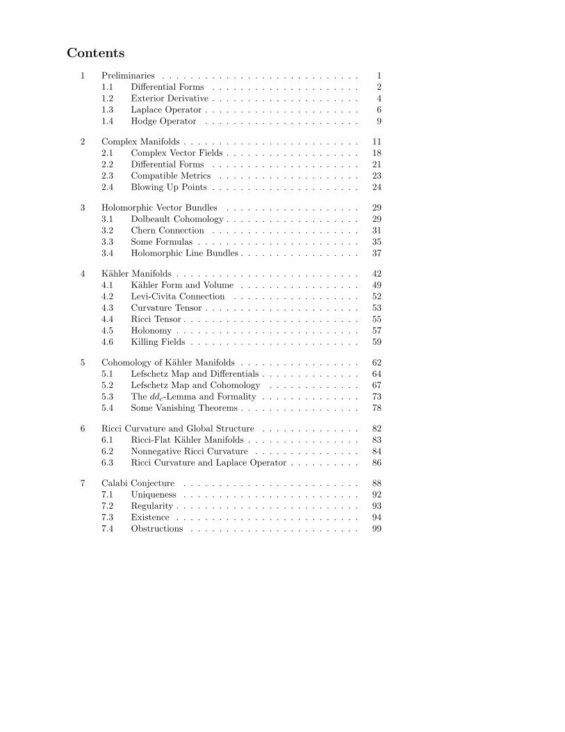
1 Preliminaries . . . . . . . . . . . . . . . . . . . . . . . . . . . . 11.1 Differential Forms . . . . . . . . . . . . . . . . . . . . . 21.2 Exterior Derivative . . . . . . . . . . . . . . . . . . . . . 41.3 Laplace Operator . . . . . . . . . . . . . . . . . . . . . . 61.4 Hodge Operator . . . . . . . . . . . . . . . . . . . . . . 9
2 Complex Manifolds . . . . . . . . . . . . . . . . . . . . . . . . . 112.1 Complex Vector Fields . . . . . . . . . . . . . . . . . . . 182.2 Differential Forms . . . . . . . . . . . . . . . . . . . . . 212.3 Compatible Metrics . . . . . . . . . . . . . . . . . . . . 232.4 Blowing Up Points . . . . . . . . . . . . . . . . . . . . . 24
3 Holomorphic Vector Bundles . . . . . . . . . . . . . . . . . . . 293.1 Dolbeault Cohomology . . . . . . . . . . . . . . . . . . . 293.2 Chern Connection . . . . . . . . . . . . . . . . . . . . . 313.3 Some Formulas . . . . . . . . . . . . . . . . . . . . . . . 353.4 Holomorphic Line Bundles . . . . . . . . . . . . . . . . . 37
4 Kahler Manifolds . . . . . . . . . . . . . . . . . . . . . . . . . . 424.1 Kahler Form and Volume . . . . . . . . . . . . . . . . . 494.2 Levi-Civita Connection . . . . . . . . . . . . . . . . . . 524.3 Curvature Tensor . . . . . . . . . . . . . . . . . . . . . . 534.4 Ricci Tensor . . . . . . . . . . . . . . . . . . . . . . . . . 554.5 Holonomy . . . . . . . . . . . . . . . . . . . . . . . . . . 574.6 Killing Fields . . . . . . . . . . . . . . . . . . . . . . . . 59
5 Cohomology of Kahler Manifolds . . . . . . . . . . . . . . . . . 625.1 Lefschetz Map and Differentials . . . . . . . . . . . . . . 645.2 Lefschetz Map and Cohomology . . . . . . . . . . . . . 675.3 The ddc-Lemma and Formality . . . . . . . . . . . . . . 735.4 Some Vanishing Theorems . . . . . . . . . . . . . . . . . 78
6 Ricci Curvature and Global Structure . . . . . . . . . . . . . . 826.1 Ricci-Flat Kahler Manifolds . . . . . . . . . . . . . . . . 836.2 Nonnegative Ricci Curvature . . . . . . . . . . . . . . . 846.3 Ricci Curvature and Laplace Operator . . . . . . . . . . 86
7 Calabi Conjecture . . . . . . . . . . . . . . . . . . . . . . . . . 887.1 Uniqueness . . . . . . . . . . . . . . . . . . . . . . . . . 927.2 Regularity . . . . . . . . . . . . . . . . . . . . . . . . . . 937.3 Existence . . . . . . . . . . . . . . . . . . . . . . . . . . 947.4 Obstructions . . . . . . . . . . . . . . . . . . . . . . . . 99
vi Contents
8 Kahler Hyperbolic Spaces . . . . . . . . . . . . . . . . . . . . . 1058.1 Kahler Hyperbolicity and Spectrum . . . . . . . . . . . 1088.2 Non-Vanishing of Cohomology . . . . . . . . . . . . . . 112
9 Kodaira Embedding Theorem . . . . . . . . . . . . . . . . . . . 1179.1 Proof of the Embedding Theorem . . . . . . . . . . . . 1199.2 Two Applications . . . . . . . . . . . . . . . . . . . . . . 123
Appendix A Chern–Weil Theory . . . . . . . . . . . . . . . . . . . . 124A.1 Chern Classes and Character . . . . . . . . . . . . . . . 130A.2 Euler Class . . . . . . . . . . . . . . . . . . . . . . . . . 135
Appendix B Symmetric Spaces . . . . . . . . . . . . . . . . . . . . . 137B.1 Symmetric Pairs . . . . . . . . . . . . . . . . . . . . . . 141B.2 Examples . . . . . . . . . . . . . . . . . . . . . . . . . . 148B.3 Hermitian Symmetric Spaces . . . . . . . . . . . . . . . 156
Appendix C Remarks on Differential Operators . . . . . . . . . . . 162C.1 Dirac Operators . . . . . . . . . . . . . . . . . . . . . . 165C.2 L2-de Rham Cohomology . . . . . . . . . . . . . . . . . 167C.3 L2-Dolbeault Cohomology . . . . . . . . . . . . . . . . . 168
Literature . . . . . . . . . . . . . . . . . . . . . . . . . . . . . . . . . 170
Index . . . . . . . . . . . . . . . . . . . . . . . . . . . . . . . . . . . 176
1 Preliminaries
In this chapter, we set notation and conventions and discuss some preliminaries.Let M be a manifold1 of dimension n. A coordinate chart for M is a tuple(x, U), where U ⊂ M is open and x : U → Rn is a diffeomorphism onto itsimage. As a rule, we will not refer to the domain U of x. The coordinate frameof a coordinate chart x consists of the ordered tuple of vector fields
Xj =∂
∂xj, 1 ≤ j ≤ n. (1.1)
We say that a coordinate chart x is centered at a point p ∈M if x(p) = 0.Let E →M be a vector bundle overM . We denote the space of sections of E
by E(E) or E(M,E). More generally, for U ⊂M open, we denote by E(U,E) thespace of sections of E over U . Furthermore, we denote by Ec(U,E) ⊂ E(U,E)the subspace of sections with compact support in U .
As long as there is no need to specify a name for them, Riemannian metricson E are denoted by angle brackets 〈· , ·〉. Similarly, if E is complex, Hermitianmetrics on E are denoted by parentheses ( · , ·). As a rule we assume thatHermitian metrics on a given bundle E are conjugate linear in the first variableand complex linear in the second. The induced Hermitian metric on the dualbundle E∗ will then be complex linear in the first and conjugate linear in thesecond variable. The reason for using different symbols for Riemannian andHermitian metrics is apparent from (1.12) below.
If E is a complex vector bundle over M and ( · , ·) is a Hermitian metric onE, then
(σ, τ)2 =
∫
M
(σ, τ) (1.2)
is a Hermitian product on Ec(M,E). We let L2(E) = L2(M,E) be the comple-tion of Ec(M,E) with respect to the Hermitian norm induced by the Hermitianproduct in (1.2) and identify L2(M,E) with the space of equivalence classes ofsquare-integrable measurable sections of E as usual2.
Let g = 〈 · , ·〉 be a Riemannian metric on M and ∇ be its Levi-Civita con-nection. By setting g(X)(Y ) := g(X,Y ), we may interpret g as an isomorphismTM → T ∗M . We use the standard musical notation for this isomorphism,
v(w) = 〈v, w〉 and 〈ϕ♯, w〉 = ϕ(w), (1.3)
where v, w ∈ TM and ϕ ∈ T ∗M have the same foot points. It is obvious that(v)♯ = v and (ϕ♯) = ϕ.
For a vector field X , the Lie derivative LXg of g measures how much gvaries under the flow of X . It is given by
(LXg)(Y, Z) = 〈∇YX,Z〉+ 〈Y,∇ZX〉. (1.4)
1Unless specified otherwise, manifolds and maps are assumed to be smooth.2We use similar terminology in the case of real vector bundles and Riemannian metrics.
2 Lectures on Kahler Manifolds
In fact, by the product rule for the Lie derivative,
X〈Y, Z〉 = LX(g(Y, Z)) = (LXg)(Y, Z) + g(LXY, Z) + g(Y, LXZ).
We say that X is a Killing field if the flow of X preserves g. By definition, Xis a Killing field iff LXg = 0 or, equivalently, iff ∇X is skew-symmetric.
1.5 Exercises. Let X be a Killing field on M .1) For any geodesic c in M , the composition X c is a Jacobi field along
c. Hint: The flow of X consists of local isometries of M and gives rise to localgeodesic variations of c with variation field X c.
2) For all vector fields Y, Z on M
∇2X(Y, Z) +R(X,Y )Z = 0.
Hint: For Y = Z, this equation reduces to the Jacobi equation.
The divergence divX of a vector field X on M measures the change of thevolume element under the flow of X . It is given by
divX = tr∇X. (1.6)
In terms of a local orthonormal frame (X1, . . . , Xn) of TM , we have
divX =∑〈∇Xj
X,Xj〉. (1.7)
By (1.4), we also havetrLXg = 2 divX. (1.8)
1.9 Divergence Formula. Let G be a compact domain in M with smoothboundary ∂G and exterior normal vector field ν along ∂G. Then
∫
G
divX =
∫
∂G
〈X, ν〉.
1.1 Differential Forms. We let A∗(M,R) := Λ∗(T ∗M) be the bundle of(multilinear) alternating forms on TM (with values in R) and A∗(M,R) :=E(A∗(M,R)) be the space of differential forms on M . We let Ar(M,R) andAr(M,R) be the subbundle of alternating forms of degree r and the subspaceof differential forms on M of degree r, respectively.
The Riemannian metric on M induces a Riemannian metric on A∗(M,R).Similarly, the Levi-Civita connection induces a connection ∇ on A∗(M,R),compare the product rule 1.20 below, and ∇ is metric with respect to theinduced metric on A∗(M,R).
Recall the interior product of a tangent vector v with an alternating formϕ with the same foot point, vxϕ = ϕ(v, . . . ), that is, insert v as first variable.There are the following remarkable relations between ∧ and x,
〈v ∧ ϕ, ψ〉 = 〈ϕ, vxψ〉 (1.10)
1 Preliminaries 3
and the Clifford relation
v ∧ (wxϕ) + wx(v ∧ ϕ) = 〈v, w〉ϕ, (1.11)
where v and w are tangent vectors and ϕ and ψ alternating forms, all with thesame foot point.
We let A∗(M,C) := A∗(M,R)⊗R C be the bundle of R-multilinear alternat-ing forms on TM with values in C and A∗(M,C) := E(A∗(M,C)) be the spaceof complex valued differential forms on M . Such forms decompose, ϕ = ρ+ iτ ,where ρ and τ are differential forms with values in R as above. We call ρ thereal part, ρ = Reϕ, and τ the imaginary part, τ = Imϕ, of ϕ and set ϕ = ρ−iτ .Via complex multilinear extension, we may view elements of A∗(M,C) as C-multilinear alternating forms on TCM = TM ⊗R C, the complexified tangentbundle.
We extend Riemannian metric, wedge product, and interior product com-plex linearly in the involved variables to TCM and A∗(M,C), respectively. Weextend ∇ complex linearly to a connection on A∗(M,C), ∇ϕ := ∇Reϕ +i∇ Imϕ. Equations 1.10 and 1.11 continue to hold, but now with complex tan-gent vectors v, w and C-valued forms ϕ and ψ. There is an induced Hermitianmetric
(ϕ, ψ) := 〈ϕ, ψ〉 (1.12)
on A∗(M,C) and a corresponding L2-Hermitian product on A∗c(M,C) as in
(1.2).Let E → M be a complex vector bundle. A differential form with values
in E is a smooth section of A∗(M,E) := A∗(M,C) ⊗ E, that is, an elementof A∗(M,E) := E(A∗(M,E)). Locally, any such form is a linear combinationof decomposable differential forms ϕ⊗ σ with ϕ ∈ A∗(M,C) and σ ∈ E(M,E).We define the wedge product of ϕ ∈ A∗(M,C) with α ∈ A∗(M,E) by
ϕ ∧ α :=∑
(ϕ ∧ ϕj)⊗ σj , (1.13)
where we decompose α =∑ϕj ⊗ σj . More generally, let E′ and E′′ be further
complex vector bundles over M and µ : E⊗E′ → E′′ be a morphism. We definethe wedge product of differential forms α ∈ A∗(M,E) and α′ ∈ A∗(M,E′) by
α ∧µ α′ :=∑
j,k
(ϕj ∧ ϕ′k)⊗ µ(σj ⊗ σ′
k) ∈ A(M,E′′), (1.14)
where we write α =∑ϕj ⊗ σj and α′ =
∑ϕ′k ⊗ σ′
k. If α and α′ are of degreer and s, respectively, then
(α ∧µ α′)(X1, . . . , Xr+s)
=1
r!s!
∑ε(σ)µα(Xσ(1), . . . , Xσ(r))⊗ α′(Xσ(r+1), . . . , Xσ(r+s)). (1.15)
4 Lectures on Kahler Manifolds
This formula shows that the wedge products in (1.13) and (1.14) do not dependon the way in which we write α and α′ as sums of decomposable differentialforms.
1.16 Exercise. Let E be a complex vector bundle over M and µ and λ becomposition and Lie bracket in the associated vector bundle EndE of endo-morphisms of E. Let α, α′, and α′′ be differential forms with values in EndE.Then
(α ∧µ α′) ∧µ α′′ = α ∧µ (α′ ∧µ α′′)
andα ∧λ α′ = α ∧µ α′ − (−1)rsα′ ∧µ α,
if α and α′ have degree r and s, respectively.
1.2 Exterior Derivative. We refer to the beginning of Appendix C for someof the terminology in this and the next subsection. Let E be a complex vectorbundle over M and D be a connection on E. For a differential form α withvalues in E and of degree r, we define the exterior derivative of α (with respectto D) by
dDα :=∑
(dϕj ⊗ σj + (−1)rϕj ∧Dσj), (1.17)
where we decompose α =∑ϕj ⊗ σj and where d denotes the usual exterior
derivative. That this is independent of the decomposition of α into a sum ofdecomposable differential forms follows from
dDα(X0, . . . , Xr) =∑
j
(−1)jDXj(α(X0, . . . , Xj , . . . , Xr))
(1.18)
+∑
j<k
(−1)j+kα([Xj , Xk], X0, . . . , Xj , . . . , Xk, . . . , Xr).
Since dD(fα)− fdDα = df ∧ α for any function f on M , the principal symbolσ : T ∗M ⊗A∗(M,E)→ A∗(M,E) of dD is given by σ(ξ ⊗ α) = ξ ∧ α.
1.19 Proposition. Let E be a vector bundle over M and D be a connectionon E. Then, for all α ∈ A∗(M,E),
dDdDα = RD ∧ε α,
where we view the curvature tensor RD of D as a two-form with values in thebundle EndE of endomorphisms of E and where the wedge product is takenwith respect to the evaluation map ε : EndE ⊗ E → E.
Via the product rule, A∗(M,E) inherits a connection D from ∇ and D,
DX(ϕ⊗ σ) := (∇Xϕ)⊗ σ + ϕ⊗ (DXσ). (1.20)
1 Preliminaries 5
In terms of D, we have
dDα =∑
X∗j ∧ DXj
α, (1.21)
where (X1, . . . , Xn) is a local frame of TM and (X∗1 , . . . , X
∗n) is the correspond-
ing dual frame. We emphasize that the curvature tensors of ∇ and D act asderivations with respect to wedge and tensor products.
Let E, E′, E′′ and µ : E ⊗ E′ → E′′ be as in (1.14). Let D, D′ and D′′ beconnections on E, E′, and E′′, respectively, such that the product rule
D′′X(µ(σ ⊗ τ)) = µ((D′
Xσ) ⊗ τ) + µ(σ ⊗ (D′′Xτ)) (1.22)
holds for all vector fields X of M . The induced connections on the bundles offorms then also satisfy the corresponding product rule,
D′′X(α ∧µ α′) = (DXα) ∧µ α′ + (α ∧µ (D′
Xα′)). (1.23)
For the exterior differential we get
dD′′
(α ∧µ α′) = (dDα) ∧µ α′ + (−1)rα ∧µ (dD′
α′), (1.24)
where we assume that α is of degree r.Let h = ( · , ·) be a Hermitian metric on E. Then h induces a Hermitian
metric on A∗(M,E), on decomposable forms given by
(ϕ⊗ σ, ψ ⊗ τ) = 〈ϕ, ψ〉(σ, τ), (1.25)
and a corresponding L2-Hermitian product on A∗c(M,E) as in (1.2).
1.26 Exercise. The analogs of (1.10) and (1.11) hold on A∗(M,E),
(v ∧ α, β) = (α, vxβ) and v ∧ (wxα) + wx(v ∧ α) = 〈v, w〉α,where v, w ∈ TM and α, β ∈ A∗(M,E) have the same foot point.
Let D be a Hermitian connection on E. Then the induced connection D onA∗(M,E) as in (1.20) is Hermitian as well.
1.27 Proposition. In terms of a local orthonormal frame (X1, . . . , Xn) of M ,the formal adjoint (dD)∗ of dD is given by
(dD)∗α = −∑
XjxDXjα.
Proof. Let α and β be differential forms of degree r − 1 and r. Let p ∈M andchoose a local orthonormal frame (Xj) around p with ∇Xj(p) = 0. Then, at p,
(dDα, β) =∑
(X∗j ∧ DXj
α, β)
=∑
(DXjα,Xjxβ)
=∑
Xj(α,Xjxβ)−∑
(α,XjxDXjβ).
The first term on the right is equal to the divergence of the complex vectorfield Z defined by (Z,W ) = (α,Wxβ), see (C.3).
6 Lectures on Kahler Manifolds
Since (dD)∗(fα) − f(dD)∗α = − gradfxα for any function f on M , theprincipal symbol σ : T ∗M ⊗A∗(M,E)→ A∗(M,E) of (dD)∗ is given by σ(ξ ⊗α) = −ξ♯xα.
1.3 Laplace Operator. As above, we let E →M be a complex vector bundlewith Hermitian metric h and Hermitian connectionD. We say that a differentialform α with values in E is harmonic if dDα = (dD)∗α = 0 and denote byH∗(M,E) the space of harmonic differential forms with values in E.
The Laplace operator associated to dD is
∆dD = dD(dD)∗ + (dD)∗dD. (1.28)
Since the principal symbol of a composition of differential operators is thecomposition of their principal symbols, the principal symbol σ of ∆dD is givenby
σ(ξ ⊗ α) = −(ξ ∧ (ξ♯xα) + ξ♯x(ξ ∧ α)) = −||ξ||2α, (1.29)
by (1.11). In particular, ∆dD is an elliptic differential operator.
1.30 Exercise. Assume that M is closed. Use the divergence formula (1.9) toshow that
(∆dDα, β)2 = (dDα, dDβ)2 + ((dD)∗α, (dD)∗β)2.
Conclude that ϕ is harmonic iff ∆dDα = 0. Compare also Corollary C.22.
Using the Clifford relation 1.11 and the formulas 1.21 and 1.27 for dD and(dD)∗, a straightforward calculation gives the Weitzenbock formula
∆dDα = −∑
j
D2α(Xj , Xj) +∑
j 6=k
X∗k ∧ (XjxR
D(Xj , Xk)α), (1.31)
where (X1, . . . , Xn) is a local orthonormal frame of TM , (X∗1 , . . . , X
∗n) is the
corresponding dual frame of T ∗M , and RD denotes the curvature tensor of theconnection D on A∗(M,E). Denoting the second term on the right hand sideof (1.31) by Kα and using (C.8), we can rewrite (1.31) in two ways,
∆dDα = − tr D2α+Kα = D∗Dα+Kα. (1.32)
Assume now that D is flat. If (Φj) is a parallel frame of E over an opensubset U of M , then over U , α ∈ A(M,E) can be written as a sum α =∑ϕj ⊗ Φj and
dDα =∑
(dϕj)⊗ Φj and (dD)∗α =∑
(d∗ϕj)⊗ Φj . (1.33)
For that reason, we often use the shorthand dα and d∗α for dDα and (dD)∗α ifD is flat. Then we also have d2 = (d∗)2 = 0, see Proposition 1.19. The latter
1 Preliminaries 7
implies that the images of d and d∗ are L2-perpendicular and that the Laplaceoperator is a square,
∆d = (d+ d∗)2. (1.34)
The fundamental estimates and regularity theory for elliptic differential oper-ators lead to the Hodge decomposition of A∗(M,E), see for example SectionIII.5 in [LM] or Chapter 6 in [Wa]:
1.35 Theorem (Hodge Decomposition). If M is closed and D is flat, then
A∗(M,E) = H∗(M,E) + d(A∗(M,E)) + d∗(A∗(M,E)),
where the sum is orthogonal with respect to the L2-Hermitian product on A∗(M,E).
In particular, if M is closed and D is flat, then the canonical map to coho-mology,
H∗(M,E)→ H∗(M,E), (1.36)
is an isomorphism of vector spaces. In other words, each de Rham cohomologyclass ofM with coefficients in E contains precisely one harmonic representative.In particular, dimH∗(M,E) <∞. The most important case is E = C.
1.37 Remark. It is somewhat tempting to assume that the ring structureof H∗(M,C) is also represented by H∗(M,C). However, this only happens inrare cases. As a rule, the wedge product of harmonic differential forms is nota harmonic differential form anymore. In fact, it is a specific property of theKahler form of a Kahler manifold that its wedge product with a harmonic formgives a harmonic form, see Theorem 5.25. Compare also Remark 1.42 below.
In the above discussion, we only considered complex vector bundles. Thereis a corresponding theory in the real case, which we will use in some instances.
1.38 Exercise. Show that for ϕ ∈ A1(M,C), the curvature term K in theWeitzenbock formula (1.32) is given by Kϕ = (Ricϕ♯), where Ric denotes theRicci tensor of M . In other words, ∆dϕ = ∇∗∇ϕ+ (Ricϕ♯).
The equation in Exercise 1.38 was observed by Bochner (see also [Ya]).In the following theorem we give his ingenious application of it. Bochner’sargument can be used in many other situations and is therefore named afterhim. Let bj(M) be the j-th Betti number of M , bj(M) = dimR H
j(M,R) =dimC H
j(M,C).
1.39 Theorem (Bochner [Boc]). Let M be a closed and connected Riemannianmanifold with non-negative Ricci curvature. Then b1(M) ≤ n with equality ifand onlyif M is a flat torus. If, in addition, the Ricci curvature of M is positivein some point of M , then b1(M) = 0.

8 Lectures on Kahler Manifolds
Proof. Since M is closed, we can represent real cohomology classes of dimensionone uniquely by harmonic one-forms, by the (identical) version of Theorem 1.35for real vector bundles. If ϕ is such a differential form, then
0 =
∫
M
〈∆dϕ,ϕ〉 =
∫
M
||∇ϕ||2 +
∫〈Ricϕ♯, ϕ♯〉,
by Exercise 1.38. By assumption, the integrand in the second integral on theright is non-negative. It follows that ϕ is parallel, therefore also the vector fieldϕ♯, and that Ricϕ♯ = 0. The rest of the argument is left as an exercise.
1.40 Remarks. 1) The earlier theorem of Bonnet–Myers makes the strongerassertion that the fundamental group of a closed, connected Riemannian man-ifold with positive Ricci curvature is finite.
2) LetM be a closed and connected Riemannian manifold with non-negativeRicci curvature. If the Ricci curvature of M is positive in some point of M ,then the Riemannian metric of M can be deformed to a Riemannian metric ofpositive Ricci curvature [Au1] (see also [Eh]).
3) The complete analysis of the fundamental groups of closed and con-nected Riemannian manifolds with non-negative Ricci curvature was achievedby Cheeger and Gromoll [CG1], [CG2]. Compare Subsection 6.1.
1.41 Exercise. Conclude from the argument in the proof of Theorem 1.39 thata closed, connected Riemannian manifold M with non-negative Ricci curvatureis foliated by a parallel family of totally geodesic flat tori of dimension b1(M).Hint: The space p of parallel vector fields on M is an Abelian subalgebra ofthe Lie algebra of Killing fields on M . The corresponding connected subgroupof the isometry group of M is closed and Abelian and its orbits foliate M byparallel flat tori.
1.42 Remark (and Exercise). The curvature operator R is the symmetricendomorphism on Λ2(TM) defined by the equation
〈R(X ∧ Y ), U ∧ V 〉 := 〈R(X,Y )V, U〉. (1.43)
Gallot and Meyer showed that the curvature term in the Weitzenbock formula(1.32) for ∆d on A∗(M,R) is positive or non-negative if R > 0 or R ≥ 0,respectively, see [GM] or (the proof of) Theorem 8.6 in [LM]. In particular,if M is closed with R > 0, then br(M) = 0 for 0 < r < n, by Hodge theoryas in (1.36) and the Bochner argument in Theorem 1.39. If M is closed withR ≥ 0, then real valued harmonic forms onM are parallel, again by the Bochnerargument. Since the wedge product of parallel differential forms is a paralleldifferential form, hence a harmonic form, this is one of the rare instances wherethe wedge product of harmonic forms is harmonic (albeit for a trivial reason),compare Remark 1.37. If M is also connected, then a parallel differential formonM is determined by its value at any given point ofM and hence br(M) ≤
(nr
)
for 0 < r < n. Equality for any such r implies that M is a flat torus.
1 Preliminaries 9
1.4 Hodge Operator. Suppose now that M is oriented, and denote by volthe oriented volume form of M . Then the Hodge operator ∗ is defined3 by thetensorial equation
∗ϕ ∧ ψ = 〈ϕ, ψ〉 vol. (1.44)
By definition, we have
∗ 1 = vol, ∗ vol = 1 and ∗ ∗ =∑
(−1)r(n−r)Pr, (1.45)
where Pr : A∗(M,R)→ Ar(M,R) is the natural projection.Let ϕ and ψ be differential forms with compact support and of degree r and
r − 1, respectively. Since d ∗ ϕ is a differential form of degree n − r + 1 andr − r2 is even, we have
∗ ∗ d ∗ ϕ = (−1)(n−r+1)(r−1)d ∗ ϕ = (−1)nr+n−r+1d ∗ ϕ.
Hence
d(∗ϕ ∧ ψ) = d ∗ ϕ ∧ ψ + (−1)n−r ∗ ϕ ∧ dψ= (−1)nr+n−r+1 ∗ (∗ d ∗ ϕ) ∧ ψ + (−1)n−r ∗ ϕ ∧ dψ= (−1)n−r(−1)nr+1〈∗ d ∗ ϕ, ψ〉+ 〈ϕ, dψ〉 vol.
(1.46)
By Stokes’ theorem, the integral over M of the left hand side vanishes. Weconclude that on differential forms of degree r
d∗ = (−1)nr ∗ d ∗ . (1.47)
It is now easy to check that∗∆d = ∆d ∗ . (1.48)
If M is closed, then ∗ maps harmonic forms to harmonic forms, by Exercise 1.30and Equation 1.48. Hence, for closed M ,
∗ : Hr(M,R)→ Hn−r(M,R) (1.49)
is an isomorphism. This is Poincare duality on the level of harmonic forms.Extend ∗ complex linearly to A∗(M,C). Let E be a vector bundle over M
and E∗ be the dual bundle of E. Assume that E is endowed with a Hermitianmetric. Via h(σ)(τ) = (σ, τ) view the Hermitian metric of E as a conjugatelinear isomorphism h : E → E∗. We obtain a conjugate linear isomorphism
∗ ⊗ h : A∗(M,E)→ A∗(M,E∗), (1.50)
where ∗ϕ := ∗ϕ. We have
((∗ ⊗ h)α) ∧ε β = (α, β) vol, (1.51)
3Note that the definition here differs from the standard one, the definition here gives amore convenient sign in (1.47).

10 Lectures on Kahler Manifolds
where ε : E∗ ⊗ E → C is the evaluation map. Note that ((∗ ⊗ h)α) ∧ε β iscomplex valued.
Let D∗ be the induced connection on E∗. With respect to D and D∗, h isa parallel morphism from E to E∗,
(D∗X(h(σ)))(τ) = X(σ, τ)− (σ,DXτ) = (DXσ, τ) = h(DXσ)(τ).
The induced (conjugate) Hermitian metric h∗ on E∗ is given by
(h(σ), h(τ)) := (σ, τ). (1.52)
Note that h∗ is complex linear in the first and conjugate linear in the secondvariable. The connection D∗ is Hermitian with respect to h∗,
X(h(σ), h(τ)) = X(σ, τ) = (DXσ, τ) + (σ,DXτ)
= (h(DXσ), h(τ)) + (h(σ), h(DXτ))
= (D∗(h(σ)), h(τ)) + (h(σ), D∗X(h(τ)).
Via ξ(h∗(η)) = (ξ, η) we consider h∗ as a conjugate linear isomorphism fromE∗to E. We have
(σ, h∗(h(τ))) = h(σ)(h∗(h(τ))) = (h(σ), h(τ)) = (σ, τ),
and hence h∗h = id. It follows that
(∗ ⊗ h∗)(∗ ⊗ h) = (∗ ⊗ h)(∗ ⊗ h∗) = (−1)r(n−r) (1.53)
on forms of degree r and n − r. Using (1.24) with D′′ the usual derivative offunctions and computing as in (1.46), we get
(dD)∗ = (−1)nr(∗ ⊗ h∗) dD∗
(∗ ⊗ h). (1.54)
This implies that the corresponding Laplacians, for simplicity denoted ∆, sat-isfy
∆ (∗ ⊗ h) = (∗ ⊗ h)∆. (1.55)
If M is closed, then ∗ ⊗ h maps harmonic forms to harmonic forms, by Ex-ercise 1.30 and Equation 1.55. Hence, for closed M , ∗ ⊗ h induces conjugatelinear isomorphisms
Hr(M,E)→ Hn−r(M,E∗). (1.56)
This is Poincare duality for vector bundle valued harmonic forms.
2 Complex Manifolds
Let V be a vector space over R. A complex structure on V is an endomorphismJ : V → V such that J2 = −1. Such a structure turns V into a complex vectorspace by defining multiplication with i by iv := Jv. Vice versa, multiplicationby i in a complex vector space is a complex structure on the underlying realvector space.
2.1 Example. To fix one of our conventions, we discuss the complex vectorspace Cm explicitly. Write a vector in Cm as a tuple
(z1, . . . , zm) = (x1 + iy1, . . . , xm + iym)
and identify it with the vector (x1, y1, . . . , xm, ym) in R2m. The correspondingcomplex structure on R2m is
J(x1, y1, . . . , xm, ym) = (−y1, x1, . . . ,−ym, xm).
We will use this identification of Cm with R2m and complex structure J onR2m without further reference.
Let M be a smooth manifold of real dimension 2m. We say that a smoothatlas A of M is holomorphic if for any two coordinate charts z : U → U ′ ⊂ Cm
and w : V → V ′ ⊂ Cm in A, the coordinate transition map z w−1 is holo-morphic. Any holomorphic atlas uniquely determines a maximal holomorphicatlas, and a maximal holomorphic atlas is called a complex structure. We saythat M is a complex manifold of complex dimension m if M comes equippedwith a holomorphic atlas. Any coordinate chart of the corresponding com-plex structure will be called a holomorphic coordinate chart of M . A Riemannsurface or complex curve is a complex manifold of complex dimension 1.
Let M be a complex manifold. Then the transition maps z w−1 of holo-morphic coordinate charts are biholomorphic. Hence they are diffeomorphismsand the determinants of their derivatives, viewed as R-linear maps, are posi-tive. It follows that a holomorphic structure determines an orientation of M ,where we choose dx1 ∧ dy1 ∧ · · · ∧ dxm ∧ dym as orientation of Cm, compareExample 2.1.
We say that a map f : M → N between complex manifolds is holomorphicif, for all holomorphic coordinate charts z : U → U ′ of M and w : V → V ′ ofN , the map w f z−1 is holomorphic on its domain of definition. We saythat f is biholomorphic if f is bijective and f and f−1 are holomorphic. Anautomorphism of a complex manifold M is a biholomorphic map f : M →M .
To be consistent in what we say next, we remark that open subsets ofcomplex manifolds inherit a complex structure. For an open subset U of acomplex manifold M , we denote by O(U) the set of holomorphic functionsf : U → C, a ring under pointwise addition and multiplication of functions.
12 Lectures on Kahler Manifolds
The inverse mapping and implicit function theorem also hold in the holo-morphic setting. Corresponding to the real case, we have the notions of holo-morphic immersion, holomorphic embedding, and complex submanifold. Thediscussion is completely parallel to the discussion in the real case.
Of course, complex analysis is different from real analysis. To state justone phenomenon where they differ, by the maximum principle a holomorphicfunction on a closed complex manifold is locally constant. In particular, Cm
does not contain closed complex submanifolds (of positive dimension).
2.2 Examples. 1) Let U ⊂ Cm be an open subset. Then M together with theatlas consisting of the one coordinate chart id : U → U is a complex manifold.
2) Riemann sphere. Consider the unit sphere
S2 = (w, h) ∈ C× R | ww + h2 = 1.
Let N = (0, 1) and S = (0,−1) be the north and south pole of S2, respectively.The stereographic projections πN : S2 \ N → C and πS : S2 \ S → C aregiven by πN (w, h) = (1− h)−1w and πS(w, h) = (1 + h)−1w, respectively. Thetransition map πS π−1
N : C \ 0 → C \ 0 is given by (πS π−1N )(z) = 1/z.
It is smooth, and thus πN and πS define a smooth atlas of S2. However, itis not holomorphic. We obtain a holomorphic atlas by replacing πS by itscomplex conjugate, πS . Then the transition map is (πS π−1
N )(z) = 1/z, andhence the atlas of S2 consisting of πN and πS is holomorphic. The Riemannsphere is S2 together with the complex structure determined by this atlas. Itis a consequence of the uniformization theorem that this complex structure onS2 is unique up to diffeomorphism. As we will see, the Riemann sphere isbiholomorphic to the complex line CP 1, described in the next example.
3) Complex projective spaces. As a set, complex projective space CPm is thespace of all complex lines in Cm+1. For a non-zero vector z = (z0, . . . , zm) ∈Cm+1, we denote by [z] the complex line generated by z and call (z0, . . . , zm)the homogeneous coordinates of [z]. For 0 ≤ j ≤ m, we let Uj = [z] ∈ CPm |zj 6= 0. Each [z] in Uj intersects the affine hyperplane zj = 1 in Cm+1 inexactly one point. We use this to obtain a coordinate map
aj : Uj → Cm, aj([z]) =
1
zj(z0, . . . , zj, . . . , zm),
where the hat indicates that zj is to be deleted. By what we said it is clearthat aj is a bijection. For j < k, the transition map aj a−1
k is defined onw ∈ Cm | wj 6= 0 and given by inserting 1 as k-th variable, multiplying theresulting (m+1)-vector by (wj)−1, and deleting the redundant j-th variable 1.Thus the transition maps are holomorphic. It is now an exercise to show thatthere is precisely one topology on CPm such that the maps aj are coordinatecharts and such that CPm together with this topology and the atlas of mapsaj is a complex manifold of complex dimension m. For m = 1, we speak of thecomplex projective line, for m = 2 of the complex projective plane.
2 Complex Manifolds 13
For m ≤ n, the map f : CPm → CPn, [z] 7→ [z, 0], is a holomorphic em-bedding. More generally, if A : Cm+1 → Cn+1 is an injective linear map, thenthe induced map f : CPm → CPn, [z] 7→ [Az], is a holomorphic embedding.Thus we can view CPm in many different ways as a complex submanifold ofCPn. We also conclude that the group PGl(m+ 1,C) = Gl(m+ 1,C)/C∗ actsby biholomorphic transformations on CPm. It is known that PGl(m+ 1,C) isactually equal to the group of biholomorphic transformations of CPm.
For the Riemann sphere S2 as in the previous example, the map f : S2 →CP 1,
f(p) =
[πN (p), 1] if p 6= N,
[1, πS(p)] if p 6= S,
is well defined and biholomorphic and thus identifies the Riemann sphere withthe complex projective line.
4) Complex Grassmannians. This example generalizes the previous one.Let V be a complex vector space of dimension n and GrV be the space ofr-dimensional complex subspaces of V , where 0 < r < n.
Let M∗ be the set of linear maps F : Cr → V of rank r. There is a canonicalprojection
π : M∗ → GrV, π(F ) = [F ] =: imF.
Let B : V → Cn be an isomorphism. Then the map
M∗ → Cn×r, F 7→ Mat(BF ),
where Mat(BF ) denotes the matrix of the linear map BF : Cr → Cn, is abijection onto the open subset of (n × r)-matrices of rank r. This turns M∗
into a complex manifold of dimension nr, and the complex structure on M∗
does not depend on the choice of B. We write
Mat(BF ) =
(F0
F1
), where F0 ∈ C
r×r and F1 ∈ C(n−r)×r,
and let UB be the subset of [F ] in GrV such that F0 has rank r. We leave itas an exercise to the reader to show that
ZB : UB → C(n−r)×r, ZB([F ]) = F1F
−10 ,
is a well defined bijection and that, for any two isomorphisms B,C : V → Cn,the transition map ZBZ−1
C is holomorphic. With the same arguments as in theprevious example we get that GrV has a unique topology such that the mapsZB are coordinate charts turning GrV into a complex manifold of complexdimension r(n − r). Moreover, π : M∗ → GrV is a holomorphic submersionand, for any isomorphism B : V → Cn,
ϕB : UB →M∗, ϕB([F ]) = B−1
(1
F1F−10
),
14 Lectures on Kahler Manifolds
where 1 stands for the r × r unit matrix and where we consider the matrix onthe right as a linear map Cr → Cn, is a holomorphic section of π.
The group Gl(r,C) of invertible matrices in Cr×r is a complex Lie group(for complex Lie groups, see Example 8 below) and, considered as group ofautomorphisms of Cr, acts on M∗ on the right,
M∗ ×Gl(r,C)→M∗, (F,A) 7→ FA.
This action is holomorphic and turns π : M∗ → GrV into a principal bundlewith structure group Gl(r,C). The complex Lie group Gl(V ) of automorphismsof V acts on M∗ and GrV on the left,
Gl(V )×M∗ →M∗, (A,F ) 7→ AF,
respectivelyGl(V )×GrV → GrV, (A, [F ]) 7→ [AF ].
These actions are also holomorphic and π is equivariant with respect to them.5) Tautological or universal bundle. Let 0 < r < n and M = GrV be
the Grassmannian of r-dimensional complex linear subspaces in V as in theprevious example. As a set, the universal bundle over GrV is equal to
UrV = (W,w) |W ∈ GrV,w ∈W.
There is a canonical projection
π : UrV → GrV, (W,w) 7→W.
For each W ∈ GrV , the bijection π−1(W ) ∋ (W,w) 7→ w ∈ W turns the fiberπ−1(W ) into an r-dimensional complex vector space isomorphic to W .
Let B : V → Cn be an isomorphism and UB ⊂ GrV be as in the previousexample. Define a bijection
ΦB : UB × Cr → π−1(UB), ΦB([F ], v) = ([F ], ϕB([F ])v),
where ϕB is as in the previous example. For each [F ] ∈ UB, the map
Cr → π−1([F ]), v 7→ ΦB([F ], v),
is an isomorphism of vector spaces. With arguments similar to the ones in theprevious examples it follows that UrV is a complex manifold in a unique waysuch that π : UrV → GrV is a complex vector bundle over GrV and such thatthe trivializations ΦB as above are holomorphic. In particular, the complexdimension of UrV is r(n − r + 1) and π is holomorphic. Moreover, the leftaction of Gl(V ) on GrV extends canonically to a holomorphic action on UrV ,
Gl(V )× UrV → UrV, (A, (W,w)) 7→ (AW,Aw).
2 Complex Manifolds 15
This action has two orbits: the set of pairs (W,w) with w 6= 0 and of pairs(W, 0).
6) Complex tori. Choose an R-basis B = (b1, . . . , b2m) of Cm. Let Γ ⊂ Cm
be the lattice consisting of all integral linear combinations of B, a discretesubgroup of the additive group Cm. Then Γ acts by translations on Cm,
(k, z) 7→ tk(z) := k + z.
This action is free and properly discontinuous. For each fixed k ∈ Γ, thetranslation tk : Cm → Cm is biholomorphic. Hence the quotient T = Γ\Cminherits the structure of a complex manifold such that the covering map Cm →T is holomorphic. Now T is diffeomorphic to the 2m-fold power of a circle,hence T with the above complex structure is called a complex torus. We alsonote that addition T ×T → T , (z, w) 7→ z+w, is well defined and holomorphicand turns T into a complex Lie group as in Example 8 below.
Let T = Γ\Cm be a complex torus and f : T → T be a biholomorphic map.Then any continuous lift g : Cm → Cm of f is Γ-equivariant and biholomorphic.Continuity implies that there is a constant C such that |g(z)| ≤ C(1+|z|) for allz ∈ Cm. By a standard result from complex analysis, g is affine. Hence f is ofthe form f(z) = Az+b with b ∈ T and A ∈ Gl(m,C) such that A(Γ) = Γ. Viceversa, for any such A ∈ Gl(m,C) and b ∈ T , the map f : T → T , f(z) = Az+b,is well defined and biholomorphic.
A one-dimensional complex torus is called an elliptic curve. It follows fromthe uniformization theorem that any complex curve diffeomorphic to the torusS1 × S1 is an elliptic curve. In particular, the complex structure described inthe next example turns S1 × S1 into an elliptic curve.
7) Hopf manifold (complex structures on S2m−1 × S1). Let m ≥ 1 andz ∈ C be a non-zero complex number of modulus |z| 6= 1. Then Z acts freelyand properly discontinuously on Cm \ 0 by (k, v) 7→ zk · v. The quotientM = (Cm \ 0)/Z is called a Hopf manifold. It is an exercise to show that Mis diffeomorphic to S2m−1 × S1. (Hint: Consider the case z = 2 first.) Sincemultiplication by zk is biholomorphic, M inherits from Cm \ 0 the structureof a complex manifold.
A generalization of this example is due to Calabi and Eckmann, who showedthat the product of odd-dimensional spheres carries a complex structure, see[CE] (Example 2.5 in [KN, Chapter IX]).
8) Complex Lie groups. As an open subset of Cn×n, the general linear groupG = Gl(n,C) is a complex manifold of complex dimension n2, and multipli-cation G × G → G and inversion G → G are holomorphic maps. The speciallinear group Sl(n,C) ⊂ Gl(n,C) is a complex Lie subgroup of complex codimen-sion 1. If V is a complex vector space of dimension n, then any isomorphismB : V → Cn identifies the general linear group Gl(V ) of V with Gl(n,C) andturns Gl(V ) into a complex Lie group, independently of the choice of B, and thespecial linear group Sl(V ) is a complex Lie subgroup of complex codimension1.
16 Lectures on Kahler Manifolds
The unitary group U(n) is not a complex Lie group – recall that its definingequation is not holomorphic. In fact, the Lie algebra g of a complex Lie groupG is a complex vector space and the adjoint representation Ad of G is a holo-morphic map into the complex vector space of complex linear endomorphismsof g. Hence Ad is constant if G is compact. It follows that compact complexLie groups are Abelian, that is, complex tori.
For a Lie groupG, a complexification ofG consists of a complex Lie groupGC
together with an inclusion G → GC such that any smooth morphism G → H ,where H is a complex Lie group, extends uniquely to a holomorphic morphismGC → H . Clearly, if GC exists, then it is unique up to isomorphism. Forexample, Sl(n,C) is the complexification of Sl(n,R). Any connected compactLie group has a complexification [Bu, Section 27]; e.g., the complexifications ofSO(n), SU(n), and U(n) are SO(n,C), Sl(n,C), and Gl(n,C), respectively.
9) Homogeneous spaces. We say that a complex manifold M is homogeneousif the group of automorphisms of M is transitive on M . For example, if Gis a complex Lie group and H is a closed complex Lie subgroup of G, thenthe quotient G/H is in a unique way a homogeneous complex manifold suchthat the natural left action by G on G/H and the projection G → G/H areholomorphic. Flag manifolds, that is, coadjoint orbits of connected compactLie groups, are homogeneous complex manifolds. In fact, if G is a connectedcompact Lie group and Gλ is the stabilizer of some λ ∈ g∗ under the coadjointrepresentation, then the inclusion of G into its complexification GC induces anisomorphism G/Gλ → GC/Pλ, where Pλ is a suitable parabolic subgroup of GC
associated to λ, a closed complex Lie subgroup of GC, see Section 4.12 in [DK].For example, U(n)/T = Gl(n,C)/B, where T is the maximal torus of diagonalmatrices in U(n) and B is the Borel group of all upper triangular matrices inGl(n,C), the stabilizer of the standard flag in Cn. For more on flag manifolds,see Chapter 8 in [Bes].
10) Projective varieties. A closed subset V ⊂ CPn is called a (complex)projective variety if, locally, V is defined by a set of complex polynomial equa-tions. Outside of its singular locus, that is, away from the subset where thedefining equations do not have maximal rank, a projective variety is a complexsubmanifold of CPn. We say that V is smooth if its singular locus is empty.A well known theorem of Chow says that any closed complex submanifold ofCPn is a smooth projective variety, see [GH, page 167].
We say that V is a rational curve if V is smooth and biholomorphic toCP 1. For example, consider the complex curve C = [z] ∈ CP 2 | z2
0 = z1z2in CP 2, which is contained in U1 ∪ U2. On U1 ∩ C we have z2/z1 = (z0/z1)
2,hence we may use u1 = z0/z1 as a holomorphic coordinate for C on U1 ∩ C.Similarly, on U2 ∩ C we have z1/z2 = (z0/z2)
2 and we may use u2 = z0/z2 asa holomorphic coordinate for C on U2 ∩ C. The coordinate transformation onU1 ∩ U2 ∩ C is u2 = 1/u1. Thus C is biholomorphic to CP 1 and hence is arational curve in CP 2. In this example, the defining equation has degree two.
2 Complex Manifolds 17
The map CP 1 ∋ [1, z] 7→ [1, z, z2, . . . , zm] ∈ CPm extends to a holomorphicembedding of CP 1 into CPm, and the maximal degree of the obvious definingequations of the image is m.
LetM be a complex manifold. We say that a complex vector bundle E →Mis holomorphic if E is equipped with a maximal atlas of trivializations whosetransition functions are holomorphic. Such an atlas turns E into a complexmanifold such that the projection E →M is holomorphic.
2.3 Examples. 1) The tangent bundle TM together with its complex structureJ is a complex vector bundle over M . The usual coordinates for the tangentbundle have holomorphic transition maps and thus turn TM into a complexmanifold and holomorphic vector bundle over M .
2) If E → M is holomorphic, then the complex tensor bundles associatedto E are holomorphic. For example, the dual bundle E∗ is holomorphic. Notehowever that TM ⊗R C is not a holomorphic vector bundle over M in anynatural way.
3) Let E → M be a holomorphic vector bundle and f : N → M be aholomorphic map. Then the pull back f∗E → N is holomorphic.
4) The universal bundle UrV → GrV is holomorphic.
Let (z, U) be a holomorphic coordinate chart of M . As usual, we let zj =xj+ iyj and write the corresponding coordinate frame as (X1, Y1, . . . , Xm, Ym).For p ∈ U , we define a complex structure Jp on TpM by
JpXj(p) = Yj(p), JpYj(p) = −Xj(p). (2.4)
Since the transition maps of holomorphic coordinate charts are holomorphic, Jpis independent of the choice of holomorphic coordinates. We obtain a smoothfield J = (Jp) of complex structures on TM .
Vice versa, if M is a smooth manifold of real dimension 2m, then a smoothfield J = (Jp) of complex structures on TM is called an almost complex struc-ture of M . An almost complex structure J = Jp is called a complex structure ifit comes from a complex structure on M as in (2.4) above. Any almost complexstructure on a surface is a complex structure (existence of isothermal coordi-nates). A celebrated theorem of Newlander and Nirenberg [NN] says that analmost complex structure is a complex structure if and only if its Nijenhuistensor or torsion N vanishes, where, for vector fields X and Y on M ,
N(X,Y ) = 2[JX, JY ]− [X,Y ]− J [X, JY ]− J [JX, Y ]. (2.5)
For an instructive discussion of the Newlander–Nirenberg theorem and its proof,see [Ka2, Section 6.3].
2.6 Exercises. 1) N is a tensor. Compare also Exercises 2.15 and 2.32.2) Let ∇ be a torsion free connection and J be an almost complex structure
on M . Show that
1
2N(X,Y ) = ∇J(JX, Y )− J∇J(X,Y )−∇J(JY,X) + J∇J(Y,X)
18 Lectures on Kahler Manifolds
to conclude that J is a complex structure if ∇J = 0.
2.7 Example. In the normed division algebra Ca of Cayley numbers 4, considerthe sphere S6 of purely imaginary Cayley numbers of norm one. For a pointp ∈ S6 and tangent vector v ∈ TpS6, define
Jpv := p · v,
where the dot refers to multiplication in Ca. Since p is purely imaginary oflength one, p · (p · x) = −x for all x ∈ Ca. It follows that Jpv ∈ TpS6 and that
J2pv = p · (p · v) = −v.
Hence J = (Jp) is an almost complex structure on S6. Since |x · y| = |x| · |y|for all x, y ∈ Ca and p ∈ S6 has norm one, J is norm preserving.
By parallel translation along great circle arcs through p, extend v to a vectorfield V in a neighborhood of p in S6. Then V is parallel at p. Along the greatcircle arc cos t ·p+sin t ·u in the direction of a unit vector u in TpS
6, the vectorfield JV is given by (cos t · p+ sin t · u) · V (cos t · p+ sin t · u). Hence
dJV (u) = u · v + p · dV (u) = u · v + p · S(u, v),
where S denotes the second fundamental form of S6. For v, w ∈ TpS6, we get
N(v, w) = 2(p · v) · w − (p · w) · v − p · (v · w) + p · (w · v) = 4[p, v, w],
where [x, y, z] = (x · y) · z − x · (y · z) denotes the associator of x, y, z ∈ Ca. Weconclude that N 6= 0 and hence that J does not come from a complex structureon S6. It is a famous open problem whether S6 carries any complex structure.
2.8 Exercise. View the sphere S2 as the space of purely imaginary quaternionsof norm one and discuss the corresponding almost complex structure on S2.
2.1 Complex Vector Fields. Let V be a real vector space, and let J be acomplex structure on V . We extend J complex linearly to the complexificationVC = V ⊗R C of V ,
J(v ⊗ α) := (Jv)⊗ α. (2.9)
Then we still have J2 = −1, hence VC is the sum
VC = V ′ ⊕ V ′′ (2.10)
of the eigenspaces V ′ and V ′′ for the eigenvalues i and −i, respectively. Themaps
V → V ′, v 7→ v′ :=1
2(v − iJv), V → V ′′, v 7→ v′′ :=
1
2(v + iJv), (2.11)
4Chapter 15 in [Ad] is a good reference to Cayley numbers.
2 Complex Manifolds 19
are complex linear and conjugate linear isomorphisms, respectively, if we con-sider V together with J as a complex vector space.
Let M be a smooth manifold with an almost complex structure J andTCM = TM ⊗R C be the complexified tangent bundle. As in (2.10), we havethe eigenspace decomposition with respect to J ,
TCM = T ′M ⊕ T ′′M. (2.12)
The decomposition in (2.11) shows that T ′M and T ′′M are smooth subbundlesof the complexified tangent bundle TCM . Moreover, by (2.11) the maps
TM → T ′M, v 7→ v′, and TM → T ′′M, v 7→ v′′, (2.13)
are complex linear respectively conjugate linear isomorphisms of complex vectorbundles over M , where multiplication by i on TM is given by J .
A complex vector field of M is a section of TCM . Any such field can bewritten in the form Z = X + iY , where X and Y are vector fields of M , thatis, sections of TM . Complex vector fields act as complex linear derivations onsmooth complex valued functions. We extend the Lie bracket complex linearlyto complex vector fields,
[X + iY, U + iV ] := [X,U ]− [Y, V ] + i([X,V ] + [Y, U ]). (2.14)
2.15 Exercise. The Nijenhuis tensor associated to J vanishes iff T ′M is aninvolutive distribution of TCM , that is, if [Z1, Z2] is a section of T ′M wheneverZ1 and Z2 are. And similarly for T ′′M . More precisely,
N(X,Y )′′ = −8[X ′, Y ′]′′ and N(X,Y )′ = −8[X ′′, Y ′′]′,
where X and Y are vector fields on M .
Suppose from now on that M is a complex manifold. Then TM (with com-plex multiplication defined via J) is a holomorphic vector bundle over M . Theisomorphism TM ∋ v 7→ v′ ∈ T ′M as in (2.13) turns T ′M into a holomorphicvector bundle. The bundle T ′′M is a smooth complex vector bundle over M ,but not a holomorphic vector bundle in a natural way.
Let (z, U) be a holomorphic coordinate chart for M . Write zj = xj + iyj
and set
Zj :=∂
∂zj=
1
2(Xj − iYj), Zj :=
∂
∂zj=
1
2(Xj + iYj), (2.16)
where (X1, Y1, . . . , Xm, Ym) is the coordinate frame associated to the coordi-
nates (x1, y1, . . . , xm, ym). In the notation of (2.13), Zj = X ′j and Zj = X ′′
j .Similarly, any complex vector field Z has components
Z ′ =1
2(Z − iJZ) and Z ′′ =
1
2(Z + iJZ) (2.17)
20 Lectures on Kahler Manifolds
in T ′M and T ′′M , respectively. We note that (X1, . . . , Xm) is a local holomor-phic frame for TM considered as a holomorphic vector bundle over M and that(Z1, . . . , Zm) is the corresponding local holomorphic frame of T ′M .
We say that a real vector field X on M is automorphic if the flow of Xpreserves the complex structure J of M . This holds iff the Lie derivativeLXJ = 0 or, equivalently, iff [X, JY ] = J [X,Y ] for all vector fields Y on M .The space a(M) of automorphic vector fields on M is a Lie algebra with respectto the Lie bracket of vector fields.
2.18 Proposition. A real vector field X on M is automorphic iff it is holomor-phic as a section of the holomorphic vector bundle TM . The complex structureJ turns a(M) into a complex Lie algebra.
Proof. To be automorphic or holomorphic is a local property. Hence we cancheck the equivalence of the two properties in holomorphic coordinates (z, U).Then the vector field is given by a smooth map X : U → Cm and J is given bymultiplication by i.
Let Y : U → Cm be another vector field. Then the Lie bracket of X with Yis given by dX(Y )− dY (X). Hence we get
[X, iY ] = dX(iY )− idY (X)
= ∂X(iY ) + ∂X(iY )− idY (X)
= i∂X(Y )− i∂X(Y )− idY (X)
= i∂X(Y ) + i∂X(Y )− idY (X)− 2i∂X(Y )
= i[X,Y ]− 2i∂X(Y ).
Hence [X, iY ] = i[X,Y ] iff ∂X(Y ) = 0.
2.19 Proposition. If M is a closed complex manifold. then dim a(M) <∞.
Proof. The space of holomorphic sections of a holomorphic vector bundle Eover M is precisely the kernel of the elliptic differential operator ∂ on the spaceof smooth sections of E, compare (3.4).
2.20 Remark. A celebrated theorem of Bochner and Montgomery states that,for a closed complex manifold M , the group Aut(M,J) of automorphismsf : M → M is a complex Lie group with respect to the compact-open topol-ogy5 and that a(M) is the Lie algebra of Aut(M,J), see [BM]. In particular,Aut(M,J) is either trivial, or a complex torus, or is not compact, compareExample 2.2.8.
5This is a subtle point. Without the assertion about the topology, the theorem is a trivialconsequence of Proposition 2.19. There is a corresponding common misunderstanding in thecase of isometry groups of Riemannian manifolds and of other groups of automorphisms.
2 Complex Manifolds 21
2.2 Differential Forms. As above, let V be a real vector space with complexstructure J . The decomposition of VC in (2.10) determines a decomposition ofthe space of complex valued alternating forms on VC,
ΛrV ∗C = Λr(V ′ ⊕ V ′′)∗
= ⊕p+q=r(Λp(V ′)∗ ⊗ Λq(V ′′)∗
)=: ⊕p+q=rΛp,qV ∗
C . (2.21)
Alternating forms on VC correspond to complex multilinear extensions of com-plex valued alternating forms on V . In this interpretation, Λp,qV ∗
Ccorresponds
to complex valued alternating r-forms ϕ on V , r = p+ q, such that, for α ∈ C,
ϕ(αv1, . . . , αvr) = αpαqϕ(v1, . . . , vr), (2.22)
where we view V together with J as a complex vector space as usual. To seethis, write vj = v′j + v′′j as in (2.11). We call elements of Λp,qV ∗
Calternating
forms on V of type (p, q). An alternating r-form ϕ of type (p, q) satisfies
(J∗ϕ)(v1, . . . , vr) := ϕ(Jv1, . . . , Jvr) = ip−qϕ(v1, . . . , vr), (2.23)
but this does not characterize the type. We note however that a non-zeroalternating r-form ϕ satisfies J∗ϕ = ϕ iff r is even and ϕ is of type (r/2, r/2).
Conjugation maps Λp,qV ∗C
to Λq,pV ∗C
, and Λp,pV ∗C
is invariant under conju-gation. The space of complex (p, p)-forms fixed under conjugation is the spaceof real valued forms of type (p, p).
Suppose now that M is a complex manifold with complex structure J .Note that A∗(M,C) = Λ∗T ∗
CM , where T ∗
CM = T ∗M ⊗R C is the complexified
cotangent bundle. As in (2.21), we have the decomposition
Ar(M,C) = ⊕p+q=rAp,q(M,C), (2.24)
where Ap,q(M,C) := Λp,qT ∗CM . The complex line bundle KM := Am,0(M,C)
plays a special role, it is called the canonical bundle. Smooth sections ofAp,q(M,C) are called differential forms of type (p, q), the space of such dif-ferential forms is denoted Ap,q(M,C).
Let z : U → U ′ be a holomorphic coordinate chart forM . Write zj = xj+iyj
and setdzj = dxj + idyj and dzj = dxj − idyj , (2.25)
differential forms of type (1, 0) and (0, 1), respectively. In terms of these, adifferential form ϕ of type (p, q) is given by a linear combination
∑
J,K
aJK dzJ ∧ dzK =
∑
J,K
aJK dzi1 ∧ · · · ∧ dzip ∧ dzj1 ∧ · · · ∧ dzjq , (2.26)
where J and K run over multi-indices j1 < · · · < jp and k1 < · · · < kq. Undera transformation z w−1 of holomorphic coordinates of M , we have
dzj =∑ ∂zj
∂wkdwk and dzj =
∑ ∂zj
∂wkdwk. (2.27)
22 Lectures on Kahler Manifolds
This shows that the natural trivializations by the forms dzI as above turn thebundles Ap,0(M,C) into holomorphic bundles over M . We also see that thecomplex vector bundles Ar(M,C) and Ap,q(M,C) are not holomorphic in anynatural way for 0 < r ≤ 2m and 0 < q ≤ m, respectively.
A quick computation gives
dϕ =∑(
Xj(aJK)dxj + Yj(aJK)dyj)∧ dzJ ∧ dzK
=∑(
Zj(aJK)dzj + Zj(aJK)dzj)∧ dzJ ∧ dzK
=: ∂ϕ+ ∂ϕ.
(2.28)
The type of ∂ϕ is (p + 1, q), the type of ∂ϕ is (p, q + 1), hence they are well
defined, independently of the choice of holomorphic coordinates. Now d = ∂+∂and d2 = 0. Hence by comparing types, we get
∂2 = 0, ∂2 = 0, ∂∂ = −∂∂. (2.29)
In particular, we get differential cochain complexes
· · · ∂−→ Ap,q−1(M,C)∂−→ Ap,q(M,C)
∂−→ Ap,q+1(M,C)∂−→ · · · (2.30)
whose cohomology groups Hp,q(M,C) are called Dolbeault cohomology groupsof M . Their dimensions, hp,q(M,C) = dimC H
p,q(M,C), are called Hodgenumbers of M . They are invariants associated to the complex structure of M .
The kernel Ωp(M) of ∂ on Ap,0(M,C) consists precisely of the holomor-phic sections of the holomorphic vector bundle Ap,0(M,C). These are calledholomorphic forms of degree p. By definition, Ωp(M) ∼= Hp,0(M,C). Thealternating sum
χ(M,O) :=∑
(−1)php,0(M,C) =∑
(−1)p dimC Ωp(M) (2.31)
is called the arithmetic genus of M .
2.32 Exercise. Let M be a smooth manifold with an almost complex structureJ . As in the case of complex manifolds, we have the decomposition
Ar(M,C) = ⊕p+q=rAp,q(M,C)
into types. If ϕ is a smooth complex valued function, that is ϕ ∈ A0(M,C),then we can decompose as in the case of complex manifolds,
dϕ = d1,0ϕ+ d0,1ϕ ∈ A1,0(M,C) +A0,1(M,C),
where d1,0 = ∂ and d0,1 = ∂ if J is a complex structure. However, if ϕ is oftype (1, 0), then a new term may arise,
dϕ = d1,0ϕ+ d0,1ϕ+ d−1,2ϕ ∈ A2,0(M,C) +A1,1(M,C) +A0,2(M,C),
2 Complex Manifolds 23
and similarly for ϕ ∈ A0,1(M,C). Show that d−1,2 is a tensor field and that
ϕ(N(X,Y )) = 8 · d−1,2ϕ(X,Y )
for all ϕ ∈ A1,0(M,C) and vector fields X,Y on M . Any differential form islocally a finite sum of decomposable differential forms. Conclude that
dϕ ∈ Ap+2,q−1(M,C) +Ap+1,q(M,C) +Ap,q+1(M,C) +Ap−1,q+2(M,C)
for any differential form ϕ of type (p, q). Which parts of dϕ are tensorial in ϕ?
2.3 Compatible Metrics. Let M be a complex manifold with correspondingcomplex structure J . We say that a Riemannian metric g = 〈· , ·〉 is compatiblewith J if
〈JX, JY 〉 = 〈X,Y 〉 (2.33)
for all vector fields X,Y on M . A complex manifold together with a compatibleRiemannian metric is called a Hermitian manifold 6 .
Let M be a complex manifold as above. If g is a compatible Riemannianmetric on M , then the complex bilinear extension of g to TCM , also denoted gor 〈· , ·〉, is symmetric and satisfies the following three conditions:
〈Z1, Z2〉 = 〈Z1, Z2〉;〈Z1, Z2〉 = 0 for Z1, Z2 in T ′M ; (2.34)
〈Z,Z〉 > 0 unless Z = 0.
Vice versa, a symmetric complex bilinear form 〈· , ·〉 on TCM satisfying thesethree conditions is the complex bilinear extension of a Riemannian metric sat-isfying (2.33). Then (2.33) also holds for the complex linear extension of J toTCM and complex vector fields X and Y .
2.35 Proposition. Let M be a complex manifold with complex structure J .Then a Riemannian metric g = 〈· , ·〉 is compatible with J iff about each pointp0 ∈M , there are holomorphic coordinates
z = (z1, . . . , zm) = (x1 + iy1, . . . , xm + iym)
such that the associated coordinate frame (X1, Y1, . . . , Xm, Ym) satisfies
〈Xj , Xk〉(p0) = 〈Yj , Yk〉(p0) = δjk and 〈Xj , Yk〉(p0) = 0.
The proof of Proposition 2.35 is straightforward and left as an exercise. Wenote the following immediate consequence.
6The usual arguments give the existence of compatible Riemannian metrics.
24 Lectures on Kahler Manifolds
2.36 Corollary. Let M be a Hermitian manifold. Then the type decomposition
Ar(M,C) = ⊕p+q=rAp,q(M,C)
is orthogonal with respect to the induced Hermitian metric (ϕ, ψ) = 〈ϕ, ψ〉. Inparticular, ∗ϕ has type (m− q,m− p) if ϕ has type (p, q).
Proof. The first assertion is clear from Proposition 2.35. The second assertionfollows from the first since the volume form has type (m,m)7.
2.4 Blowing Up Points. Consider the universal bundle U1Cm over CPm−1.The restriction of the map U1Cm → Cm, (L, z) 7→ z, to the open subset(L, z) ∈ U1Cm | z 6= 0 is biholomorphic onto Cm \ 0. Thus we can thinkof U1C
m as Cm, where the point 0 is replaced by the set (L, 0) ∈ U1Cm.We identify the latter with CPm−1 and thus have blown up the point 0 of Cm
to CPm−1. A similar construction can be carried out for points in complexmanifolds.
2.37 Remark. For any r > 0, we can identify Sr = (L, z) ∈ U1Cm | |z| = rwith the sphere of radius r in Cm. Then the projection π : Sr → CPm−1 turnsinto the Hopf fibration: The fibers of π intersect Sr in Hopf circles, that is,the intersections of complex lines in Cm with the sphere Sr. Renormalizing thegiven Riemannian metric on Sr (of sectional curvature 1/r2) by adding the pullback of any fixed Riemannian metric g on CPm−1, we obtain a Riemannianmetric gr on the sphere S2m−1. We can think of (S2m−1, gr) as a collapsingfamily of Riemannian manifolds with limit (CPm−1, g), as r → 0. The differen-tial geometric significance of this kind of collapse was first recognized by Berger:The sectional curvature of the collapsing spheres stays uniformly bounded asr → 0, see Example 3.35 in [CE], [Kar, page 221], and [CGr].
Let M be a complex manifold and p be a point in M . The blow up of Mat p replaces p by the space of complex lines in TpM . The precise constructiongoes as follows. Let z = (z1, . . . , zm) : U → U ′ be holomorphic coordinatesabout p with z(p) = 0. In U ′ × CPm−1, consider the set
V = (z, [w]) | ziwj = zjwi for all i, j,where points in CPm−1 are given by their homogeneous coordinates, denoted[w]. On the subset wj 6= 0 of CPm−1, V is defined by the m−1 independentequations
zi =wi
wjzj , i 6= j,
the other equations follow. Hence the system of equations defining V hasconstant rank m− 1, and hence V is a complex submanifold of U ′×CPm−1 ofdimension m with
S = V ∩ z = 0 ∼= CPm−1.
7Recall that dz ∧ dz = −2idx ∧ dy.
2 Complex Manifolds 25
On V \ S, [w] is determined by z, hence
V \ S ∼= U \ p.
More precisely, the canonical map
V \ S → U ′ \ 0, (z, [w]) 7→ z,
is biholomorphic. We use it to glue V to M \p and obtain a complex manifoldM , the blow up of M at p, together with a holomorphic map
π : M →M
such that π−1(p) = S and π : M \ S →M \ p is biholomorphic.We consider V as an open subset of M . Choose ε > 0 such that the image
U ′ of the holomorphic coordinates z contains the ball of radius ε > 0 about 0in Cm. Then the map
Vε := (z, [w]) ∈ V | |z| < ε → (L, z) ∈ U1Cm | |z| < ε,
(z, [w]) 7→ ([w], z),
is biholomorphic. Hence a neighborhood of S in M is biholomorphic to aneighborhood of the zero-section of U1Cm such that the map σ : Vε → CPm−1,σ(z, [w]) = [w], corresponds to the projection. For any r ∈ (0, ε), the set
Sr = (z, [w]) ∈ V | |z| = r
corresponds to the sphere of radius r in Cm. The fibers of π intersect Sr in Hopfcircles, that is, the intersections of complex lines in Cm with Sr. Thus we canagain think of π : Sr → CPm−1 as the Hopf fibration and of the convergenceSr → S, as r → 0, as the collapse of S2m−1 to CPm−1 along Hopf circles;compare with Remark 2.37 above.
2.38 Exercises. Let M be the blow up of M at p as above.1) Let z = f(z) be other holomorphic coordinates of M about p with z(p) =
0, and let M be the blow up of M at p with respect to the coordinates z. Writef(z) =
∑fj(z)z
j, where the maps fj are holomorphic with fj(0) = ∂jf(0).Show that
f(z, [w]) =“
f(z),h∑
fj(z)wj
i”
extends the identity on M \p to a biholomorphic map M → M . In this sense,the blow up of M at p does not depend on the choice of centered holomorphiccoordinates.
2) Let f : M → N be a holomorphic map, where N is another complexmanifold. If f is constant on S, then there is a holomorphic map f : M → Nsuch that f = f π.
26 Lectures on Kahler Manifolds
2.39 Remark. By replacing centered holomorphic coordinates about p by atubular neighborhood of the zero section in the normal bundle, there is a ratherimmediate generalization of the blow up of points to a blow up of complexsubmanifolds, see e.g. Section 4.6 in [GH] or Section 2.5 in [Hu].
2.40 Examples. 1) Kummer surface. In this example it will be convenientto enumerate coordinates by subindices. Consider the quotient Q = C2/Z2,where Z2 = 1,−1 acts by scalar multiplication on C2. Let q0 be the imageof 0 under the natural projection C2 → Q. Note that away from 0 and q0,respectively, the projection is a twofold covering with holomorphic coveringtransformations, turning Q \ q0 into a complex manifold. Via
z0 = t1t2, z1 = t21, z2 = t22,
we can identify Q with the algebraic hypersurface
H = (z0, z1, z2) ∈ C3 | z2
0 = z1z2 ⊂ C3,
which has a singularity at the origin 0. We blow up C3 at 0 to get
C3 = (z, [w]) ∈ C
3 × CP 2 | ziwj = zjwi.
We haveπ−1(H \ 0) = (z, [w]) ∈ C
3 | z 6= 0, w20 = w1w2.
In particular, the closure of π−1(H \ 0) in C3 is the regular hypersurface
H = (z, [w]) ∈ C3 | w2
0 = w1w2 ⊂ C3.
Thus by blowing up 0 ∈ C3, we resolved the singularity of H .Recall that C = [w] ∈ CP 2 | w2
0 = w1w2 is an embedded CP 1, com-pare Example 2.2.10. There is a natural projection H → C. We choose(uj , zj) as holomorphic coordinates for H over the preimage of Uj under thisprojection. The coordinate transformation over the preimage of U1 ∩ U2 is(u2, z2) = (u−1
1 , u21z1). The holomorphic cotangent bundle A1,0(C,C) has
duj as a nowhere vanishing section over Uj , and du2 = −u−21 du1 over U1 ∩
U2. We conclude that the identification (u1, z1du1) ↔ (u1, z1) over U1 and(u2,−z2du2) ↔ (u2, z2) over U2 establishes a biholomorphic map between Hand A1,0(C,C) = A1,0(CP 1,C).
Let T 4 = Z4\C2. Scalar multiplication by Z2 on C2 descends to an actionof Z2 on T 4. This action has 16 fixed points, namely the points with integralor half-integral coordinates in T 4. At each fixed point x ∈ T 4, the action islocally of the form ±1 · (x + t) = x ± t as above. Thus we can resolve eachof the quotient singularities on T 4/Z2 by the above construction and obtain acompact complex surface, the Kummer surface. For more information on the
Kummer surface we refer to [Jo, Section 7.3].
2 Complex Manifolds 27
2) Dependence of blow-up on points.8 Let m ≥ 2 and T = Γ\Cm be a com-plex torus. Let (p1, . . . , pk) and (p′1, . . . , p
′l) be two tuples of pairwise different
points in T . Let M and M ′ be the blow ups of T in the points p1, . . . , pk andp′1, . . . , p
′l, respectively, and let π : M → T and π′ : M ′ → T be the projections.
Let Si and S′j be the preimages of pi and p′j under π and π′, respectively.
Let f : M → M ′ be a holomorphic map. Since Si ∼= CPm−1 is simplyconnected, the restriction of π′ f to Si lifts to a holomorphic map Si → Cm.Now Si is a closed complex manifold, hence any such lift is constant. It followsthat π′ f maps Si to a point in T . In particular, there is a holomorphic mapg : T → T such that π′ f = g π.
Suppose now that f is biholomorphic. Then f is not constant on Si (weassume m ≥ 2). By what we said above, it follows that f maps each Sibiholomorphically to an S′
j . Thus k = l and, up to renumeration, f(Si) = S′i
for all i. Moreover, the induced map g : T → T is biholomorphic with g(pi) = p′ifor all i.
Let now k = l = 2, p1 = p′1 = 0, p2 = p, p′2 = p′. In Example 2.2.6 abovewe showed that any biholomorphic map of T is of the form h(z) = Az+ b withb ∈ T and A ∈ Gl(m,C) such that A(Γ) = Γ. Hence the above g is of the formg(z) = Az for some A ∈ Gl(m,C) with A(Γ) = Γ and Ap = p′ (in T ). Onthe other hand, there are pairs of points p, p′ ∈ T \ 0 such that there is noA ∈ Gl(m,C) with A(Γ) = Γ and Ap = p′. Then by what we just said, thecorresponding blow ups M and M ′ of T in 0, p and 0, p′, respectively, are notbiholomorphic.
2.41 Exercise. In terms of oriented smooth manifolds, the blow up M of M atp ∈M corresponds to the connected sum M#CP
m, where CP
mdenotes CPm
with orientation opposite to the standard one: Choose w/w0 as a coordinateabout q = [1, 0, . . . , 0] in U0 = [w0, w] | w0 6= 0 ⊂ CPm. Let ε > 0 andVε ⊂ M be as above. Set
U ′ε = [w0, w] ∈ CP
m | |w0| < ε|w|.
Use coordinates z about p as in the definition of blow ups and w/w0 as aboveto define the connected sum M#CP
m. Then the map f : M#CP
m → M ,
f(p′) =
p′ if p′ ∈M \ p,(w0w/|w|2, [w]) ∈ Vε if p′ = [w0, w] ∈ U ′
ε,
is well defined and an orientation preserving diffeomorphism. In particular, asa smooth manifold, the blow up M does not depend on the choice of p ∈M .
We conclude our discussion of blow ups with a fact on the automorphismgroup of a compact complex surface which we cannot prove in the framework
8I owe this example to Daniel Huybrechts.
28 Lectures on Kahler Manifolds
of these lecture notes, but which will provide us with an important example inSubsection 7.4. For a closed complex manifold M with complex structure J ,denote by Aut(M) = Aut(M,J) the group of biholomorphic transformations ofM , endowed with the compact-open topology, and by Aut0(M) the componentof the identity in Aut(M).
2.42 Proposition. Let M be a compact complex surface and π : Mp → Mbe the blow up of M in p ∈ M . Then automorphisms in Aut0(Mp) leave theexceptional divisor S = π−1(p) invariant and, via restriction to M \ S,
Aut0(Mp) ∼= Φ ∈ Aut0(M) | Φ(p) = p =: Aut0(M,p).
The action of Φ ∈ Aut0(M,p) on S ∼= P (TpM) is induced by dΦp.
The only issue is to show that an automorphism of Mp in Aut0(Mp) leavesS invariant. Given some facts about topological intersection properties of ana-lytic cycles, the proof of this is actually quite simple and geometric, see [GH],Chapter 4.1. A corresponding statement would be wrong for the full automor-phism group, since ifM itself is already a blow up, there may be automorphismspermuting the various exceptional divisors.
2.43 Example. Consider the blow up of CP 2 in one or two points, which wechoose to be [1, 0, 0] and [1, 0, 0], [0, 1, 0], respectively. By Proposition 2.42, therespective automorphism groups are
1 ∗ ∗0 ∗ ∗0 ∗ ∗
∈ Gl(3,C)
and
1 0 ∗0 ∗ ∗0 0 ∗
∈ Gl(3,C)
. (2.44)
For a blow up of CP 2 in three points, the automorphism group, and hencethe complex structure, clearly depends on the choice of points, i.e., on whetherthey are in general position or not.
3 Holomorphic Vector Bundles
Let E → M be a holomorphic vector bundle. For U ⊂ M open, we denote byO(U,E) the space of holomorphic sections of E over U , a module over the ringO(U). If (Φ1, . . . ,Φk) is a holomorphic frame of E over U , then
O(U)k ∋ ϕ 7→ ϕµΦµ ∈ O(U,E) (3.1)
is an isomorphism.
3.1 Dolbeault Cohomology. We now consider differential forms on M withvalues in E. Since M is complex, we can distinguish forms according to theirtype as before,
Ar(M,E) =∑
p+q=r
Ap,q(M,E), (3.2)
where Ap,q(M,E) = Ap,q(M,C)⊗E. With respect to a local holomorphic frameΦ = (Φj) of E, a differential form of type (p, q) with values in E is a linearcombination
α = ϕj ⊗ Φj , (3.3)
where the coefficients ϕj are complex valued differential forms of type (p, q).The space of such differential forms is denoted Ap,q(M,E). We define the
∂-operator on differential forms with values in E by
∂α := (∂ϕj)⊗ Φj . (3.4)
Since the transition maps between holomorphic frames of E are holomorphic,it follows that ∂α is well defined. By definition, ∂α is of type (p, q + 1). We
have ∂∂ = 0 and hence
· · · ∂−→ Ap,q−1(M,E)∂−→ Ap,q(M,E)
∂−→ Ap,q+1(M,E)∂−→ · · · (3.5)
is a cochain complex. The cohomology of this complex is denoted Hp,∗(M,E)and called Dolbeault cohomology of M with coefficients in E. The dimensions
hp,q(M,E) := dimC Hp,q(M,E) (3.6)
are called Hodge numbers of M with respect to E.
3.7 Remark. Let Ωp(E) be the sheaf of germs of holomorphic differentialforms with values in E and of degree p (that is, of type (p, 0)). Let Ap,q(E)be the sheaf of germs of differential forms with values in E and of type (p, q).Then
0→ Ωp(E) → Ap,0(E)∂−→ Ap,1(E)
∂−→ Ap,2(E)∂−→ · · ·
is a fine resolution of Ωp(E). HenceHq(M,Ωp(E)) is isomorphic toHp,q(M,E).
30 Lectures on Kahler Manifolds
We are going to use the notation and results from Chapter 1. We assumethat M is endowed with a compatible metric in the sense of (2.33) and thatE is endowed with a Hermitian metric. Then the splitting of forms into typesas in (3.2) is perpendicular with respect to the induced Hermitian metric onA∗(M,E).
Suppose that α and β are differential forms with values in E and of type(p, q) and (p, q − 1), respectively. By Corollary 2.36, (∗ ⊗ h)α is of type (m −p,m − q). Therefore ((∗ ⊗ h)α) ∧ε β is a complex valued differential form oftype (m,m− 1). It follows that
∂(((∗ ⊗ h)α) ∧ε β
)= d(((∗ ⊗ h)α) ∧ε β
).
Since the real dimension of M is 2m, we have (∗⊗h∗)(∗⊗h) = (−1)r on formsof degree r = p+ q. Computing as in (1.46), we get
d(((∗ ⊗ h)α) ∧ε β
)= ∂
(((∗ ⊗ h)α) ∧ε β
)
= (−1)2m−r−((∗ ⊗ h∗)∂(∗ ⊗ h)α, β) + (α, ∂β) vol.
It follows that∂∗ = (∗ ⊗ h∗)∂(∗ ⊗ h). (3.8)
Here the ∂-operator on the right belongs to the dual bundle E∗ of E. Let
∆∂
= ∂∂∗ + ∂∗∂ (3.9)
be the Laplace operator associated to ∂. We claim that
∆∂
(∗ ⊗ h) = (∗ ⊗ h)∆∂, (3.10)
where the Laplace operator on the left belongs to E∗. In fact,
∆∂
(∗ ⊗ h) = ∂(∗ ⊗ h)∂(∗ ⊗ h∗)(∗ ⊗ h) + (∗ ⊗ h)∂(∗ ⊗ h∗)∂(∗ ⊗ h)= (∗ ⊗ h)∂(∗ ⊗ h∗)∂(∗ ⊗ h) + (∗ ⊗ h)(∗ ⊗ h∗)∂(∗ ⊗ h)∂= (∗ ⊗ h)∆
∂.
We denote by Hp,q(M,E) the space of ∆∂-harmonic forms of type (p, q) with
coefficients in E. By (3.10), ∗ ⊗ h restricts to a conjugate linear isomorphism
Hp,q(M,E)→ Hm−p,m−q(M,E∗). (3.11)
In the rest of this subsection, suppose that M is closed. Then by Hodge theory,the canonical projectionHp,q(M,E)→ Hp,q(M,E) is an isomorphism of vectorspaces. From (3.11) we infer Serre duality, namely that ∗⊗h induces a conjugatelinear isomorphism
Hp,q(M,E)→ Hm−p,m−q(M,E∗). (3.12)
In particular, we have hp,q(M,E) = hm−p,m−q(M,E∗) for all p and q.
3.13 Remark. Equivalently we can say that ∗ ⊗ h induces a conjugate linearisomorphism Hq(M,Ωp(E)) ∼= Hm−q(M,Ωm−p(E∗)), see Remark 3.7.
3 Holomorphic Vector Bundles 31
3.2 Chern Connection. Let D be a connection on E and σ a smooth sectionof E. Then we can split
Dσ = D′σ +D′′σ (3.14)
with D′σ ∈ A1,0(M,E) and D′′σ ∈ A0,1(M,E). Let (Φ1, . . . ,Φk) be a holo-morphic frame of E over an open subset U ⊂M . Then
DΦµ = θνµΦν , (3.15)
where θ = (θνµ) is the connection form and θνµΦν is shorthand for θνµ ⊗ Φν .
3.16 Lemma. D′′σ = 0 for all local holomorphic sections σ of E iff D′′ = ∂.Then the connection form θ ∈ A1,0(U,Ck×k).
Proof. The assertion follows from comparing types in
D′σ +D′′σ = Dσ = dϕµΦµ + ϕµDΦµ = ((∂ + ∂)ϕµ + ϕνθµν )Φµ,
where σ = ϕµΦµ in terms of a local holomorphic frame (Φµ) of E.
3.17 Lemma. Let h = ( · , ·) be a smooth Hermitian metric on E. If D′′ = ∂,then D is Hermitian iff
(σ,D′Xτ) = ∂(σ, τ)(X) or, equivalently, (D′
Xσ, τ) = ∂(σ, τ)(X)
for all vector fields X on M and local holomorphic sections σ, τ of E.
Proof. In the sense of 1-forms we write (σ,D′τ) = ∂(σ, τ) for the equality inthe lemma. If this equality holds, then
d(σ, τ) = ∂(σ, τ) + ∂(σ, τ)
= (D′σ, τ) + (σ,D′τ)
= (Dσ, τ) + (σ,Dτ),
where we use D′′σ = D′′τ = 0. Since E has local holomorphic frames, weconclude that the equality in the lemma implies that D is Hermitian. Theother direction is similar.
3.18 Theorem. Let E →M be a holomorphic vector bundle and h = ( · , ·) bea smooth Hermitian metric on E. Then there is precisely one connection D onE such that 1) D is Hermitian and 2) D′′ = ∂.
Proof. Let (Φ1, . . . ,Φk) be a holomorphic frame of E over an open subset U ⊂M and θ = (θνµ) be the corresponding connection form as in (3.15). Now 2)implies that θ is of type (1, 0). By Property 1),
dhµν = dh(Φµ,Φν) = h(θλµΦλ,Φν) + h(Φµ, θλνΦλ)
= θλµhλν + hµλθλν = hνλθλµ + hµλθ
λν .
32 Lectures on Kahler Manifolds
Now dhµν = ∂hµν + ∂hµν . Since θ is of type (1, 0), we conclude
∂hµν = hµλθλν or θ = h−1∂h, (3.19)
by comparison of types. This shows that Properties 1) and 2) determine Duniquely. Existence follows from the fact that the local connection forms θ =h−1∂h above transform correctly under changes of frames. Another argumentfor the existence is that for local holomorphic sections σ and τ of E, ∂(σ, τ)is conjugate O-linear in σ so that the equation in Lemma 3.17 leads to thedetermination of the yet undetermined D′.
The unique connection D satisfying the properties in Theorem 3.18 will becalled the Chern connection. It depends on the choice of a Hermitian metricon E.
3.20 Exercises. 1) Let E → M be a holomorphic vector bundle and h bea Hermitian metric on E. Let f : N → M be a holomorphic map. Thenthe Chern connection of the pull back Hermitian metric f∗h on the pull backf∗E → N is the pull back of the Chern connection on E with respect to h.
2) Let E →M be a holomorphic vector bundle and E′ →M be a holomor-phic vector subbundle of E. Let h be a Hermitian metric on E and h′ be therestriction of h to E′. For a section σ of E write σ = σ′ + σ′′, where σ′ is asection of E′ and σ′′ is perpendicular to E′. Let D be the Chern connectionon E with respect to h. Then the Chern connection D′ of E′ with respect toh′ is given by D′σ = (Dσ)′.
Recall that this is the standard recipe of getting a Hermitian connection fora subbundle of a Hermitian bundle with a Hermitian connection.
In what follows, we use the wedge product as defined in (1.15) and thediscussion in Example 1.16, applied to the trivial bundle E = M × Ck.
3.21 Proposition. Let E →M be a holomorphic vector bundle with Hermitianmetric h and corresponding Chern connection D. Let (Φ1, . . . ,Φk) be a localholomorphic frame of E and θ and Θ be the corresponding connection andcurvature form. Then:
1) θ = h−1∂h with h = (hµν);
2) D′ = ∂ + θ and D′′ = ∂;
3) θ is of type (1, 0) and ∂θ = −θ ∧µ θ;
4) Θ = ∂θ and Θ is of type (1, 1);
5) ∂Θ = 0 and ∂Θ = Θ ∧λ θ = Θ ∧µ θ − θ ∧µ Θ.
3 Holomorphic Vector Bundles 33
In the case of a holomorphic line bundle E →M , a local nowhere vanishingholomorphic section Φ, and h = (Φ,Φ), Proposition 3.21 gives
θ = ∂ lnh and Θ = ∂∂ lnh. (3.22)
We will use these formulas without further reference.
Proof of Proposition 3.21. The first assertion follows from the proof of Theo-rem 3.18, the second from Lemma 3.16. As for the third assertion, we have
∂θ = ∂(h−1∂h) = −(h−1∂hh−1) ∧µ ∂h= −(h−1∂h) ∧µ (h−1∂h) = −θ ∧µ θ.
In particular,
Θ = ∂θ + ∂θ + θ ∧µ θ = ∂θ.
Hence ∂Θ = 0 and, by the Bianchi identity dΘ = Θ ∧λ θ, we conclude that
Θ ∧λ θ = dΘ = ∂Θ + ∂Θ = ∂Θ.
3.23 Proposition. Let E →M be a holomorphic vector bundle with Hermitianmetric h and Chern connection D. Let p0 ∈ M and z be holomorphic coordi-nates about p0 with z(p0) = 0. Then there is a holomorphic frame (Φ1, . . . ,Φk)of E about p0 such that
1) h(z) = 1 +O(|z|2);
2) Θ(0) = ∂∂h(0).
Proof. Suppose 1) holds. Then
Θ(0) = ∂θ(0) =((∂h−1) ∧µ ∂h+ h−1∂∂h
)(0) = ∂∂h(0),
hence 1) implies 2). To show 1), we choose a holomorphic frame (Φ1, . . . ,Φk)about p0 such that hµν(0) = δµν . We define a new holomorphic frame
Φµ = Φµ + ziaνµiΦν
with aνµi = −(∂hνµ/∂zi)(0). It is easy to check that h = 1 +O(|z|2).
3.24 Example (Tautological bundle). Let M = Gr,n := GrCn and E → M
be the tautological bundle as in Example 2.2.5. The standard Hermitian innerproduct on Cn induces a Hermitian metric on E.
We identify sections of E over an open subset U of M with maps σ : U → Cn
such that σ(p) ∈ p for all p ∈ U . Then a holomorphic frame over an open subset
34 Lectures on Kahler Manifolds
U ⊂ M is given by holomorphic mappings Φµ : U → Cn, 1 ≤ µ ≤ r, such that(Φ1(p), . . . ,Φr(p)) is a basis of p, for all p ∈ U . For such a frame,
hµν = (Φµ,Φν) =∑
λ
ΦλµΦλν = (ΦtΦ)µν with Φ = (Φνµ).
If σ : U → Cm is a section of E and X is a vector field of M over U , thenthe derivative dσ(X) of σ in the direction of X need not be a section of E;that is, dσp(Xp) need not be an element of p anymore. We obtain the Chernconnection D of E by setting
(DXσ)(p) = πp(dσp(Xp)),
where πp : Cn → Cn is the orthogonal projection of Cn onto p, compare Exer-cise 3.20.2 (where the ambient bundle is M × Cn in our case).
Consider the plane p0 spanned by the first r unit vectors, in homogeneouscoordinates in Cn×r written as
p0 =
[10
]∈M,
where 1 = 1r is the r × r unit matrix. Then we get a holomorphic parameteri-zation (the inverse of holomorphic coordinates) of M about p0 by
C(n−r)×r ∋ z 7→
[1z
]∈M.
Moreover, the r columns of the matrix ( 1z ) are a holomorphic frame of E. For
this frame we have
hµν = δµν +∑
λ
zλµzλν = δµν + (ztz)µν .
In particular,
h = 1 +O(|z|2).
In z = 0, that is, in p0, we have
Θ(0) = ∂∂h(0) = ∂zt ∧ ∂z = dzt ∧ dz.
The canonical action of the group U(n) on M is transitive and extends canoni-cally to an action on E which leaves h invariant. Each element from U(n) actsbiholomorphically on M and E. In particular, choosing p0 as above means norestriction of generality.
3 Holomorphic Vector Bundles 35
3.3 Some Formulas. For the following, we refer again to notation and resultsintroduced in Chapter 1. Let E → M be a holomorphic vector bundle overM . Let h be a Hermitian metric on E and D be the corresponding Chernconnection. Then we have the associated exterior differential
dD : Ar(M,E)→ Ar+1(M,E), (3.25)
see (1.18) and (1.21). Let (Φµ) be a local holomorphic frame of E and
α = ϕµΦµ (3.26)
be a differential form with values in E of type (p, q) with p + q = r. By thecharacteristic property of the Chern connection, we have
dDα = dϕµ ⊗ Φµ + (−1)rϕµ ∧DΦµ = ∂Dα+ ∂α, (3.27)
where∂Dα := ∂ϕµ ⊗ Φµ + (−1)rϕµ ∧DΦµ. (3.28)
Note that ∂Dα and ∂α are of type (p+ 1, q) and (p, q + 1), respectively.
3.29 Proposition. Let E be a holomorphic vector bundle over M with Her-mitian metric and associated Chern connection D. Then, for any differentialform α with values in E,
(∂D)2α = (∂)2α = 0 and (∂D∂ + ∂∂D)α = (dD)2α = RD ∧ε α,
where ε : End(E)⊗ E → E is the evaluation map.
Proof. If α is a differential form with values in E of type (p, q), then dDdDα =RD ∧ε α, see Proposition 1.19. By Proposition 3.21, RD is of type (1, 1), hencedDdDα is of type (p+ 1, q + 1). By definition,
dDdDα = ∂D∂Dα+ ∂∂α+ (∂D∂ + ∂∂D)α.
The first two forms on the right hand side vanish since they have type (p+2, q)and (p, q + 2), respectively.
We assume now that, in addition, M is endowed with a compatible Rie-mannian metric as in (2.33). Let (X1, Y1, . . . , Xm, Ym) be a local orthonormalframe of M with JXj = Yj . Set
Zj =1
2(Xj − iYj) and Zj =
1
2(Xj + iYj), (3.30)
and let Z∗1 , . . . , Z
∗n, Z
∗1 , . . . , Z
∗n be the corresponding dual frame of T ∗
CM . With
our conventions, we have
Zj := 〈Zj , · 〉 =1
2Z∗j and Zj := 〈Zj , · 〉 =
1
2Z∗j . (3.31)
36 Lectures on Kahler Manifolds
Since Xj = Zj + Zj and Yj = i(Zj − Zj), we get
X∗j =
1
2(Z∗
j + Z∗j ) and Y ∗
j = − i2(Z∗
j − Z∗j )
for the dual frame (X∗1 , Y
∗1 , . . . , X
∗m, Y
∗m) of (X1, Y1, . . . , Xm, Ym). Therefore,
dD =1
2
∑(Z∗
j + Z∗j ) ∧ DZj+Zj
+ (Z∗j − Z∗
j ) ∧ DZj−Zj
=∑
Z∗j ∧ DZj
+ Z∗j ∧ DZj
= ∂D + ∂,
(3.32)
meaning that the sum of the first terms is equal to ∂D and the sum of the secondto ∂. To compute the adjoint operator (dD)∗ of dD with respect to the inducedHermitian metric as in (1.25), we note first that the relations in Exercise 1.26
also hold for complex tangent vectors. Since Z∗j = 2Zj and Z∗
j = 2Zj , we get
(dD)∗ = −2∑
ZjxDZj+ ZjxDZj
= (∂D)∗ + ∂∗, (3.33)
where we use the first relation from Exercise 1.26 for the first equality andcomparison of types for the second. The Laplace operators associated to ∂ and∂D are defined by
∆∂
= ∂∂∗ + ∂∗∂ and ∆∂D = ∂D(∂D)∗ + (∂D)∗∂D, (3.34)
respectively. Both preserve the type of forms. Using the second relation fromExercise 1.26, a straightforward computation gives the following Weitzenbockformulas,
∆∂α = −2
∑
j
D2α(Zj , Zj) + 2∑
j,k
Z∗j ∧ (Zkx(RD(Zk, Zj)α))
= −2∑
j
D2α(Zj , Zj) + 2∑
j,k
Zjx(Z∗k ∧ (RD(Zk, Zj)α)),
(3.35)
∆∂Dα = −2∑
j
D2α(Zj , Zj) + 2∑
j,k
Zjx(Z∗k ∧ (RD(Zk, Zj)α))
= −2∑
j
D2α(Zj , Zj) + 2∑
j,k
Z∗j ∧ (Zkx(RD(Zk, Zj)α)),
(3.36)
where the frame (Z1, Z1, . . . , Zm, Zm) is as in (3.30) and where RD denotes thecurvature tensor of D on A∗(M,E).
3.37 Exercises. 1) Show that, for a differential form ϕ⊗ σ of degree r,
∂D(ϕ⊗ σ) = ∂ϕ⊗ σ + (−1)rϕ ∧D′σ,
∂(ϕ⊗ σ) = ∂ϕ⊗ σ + (−1)rϕ ∧D′′σ.
3 Holomorphic Vector Bundles 37
2) Prove Formulas 3.35 and 3.36 and show that
4∑
D2α(Zj , Zj) = tr D2α+ i∑
RD(Xj , JXj)α,
4∑
D2α(Zj , Zj) = tr D2α+ i∑
RD(JXj , Xj)α.
3.4 Holomorphic Line Bundles. The results in this subsection will bemainly used in Section 9. We continue to assume that M is a complex manifold.Let E →M be a complex line bundle. Let (Uα) be an open covering of M suchthat, for each α, there is a nowhere vanishing smooth section Φα : Uα → E.If σ is a smooth section of E, then we can write σ = σαΦα over Uα, whereσα : Uα → C is a smooth function, the principal part of σ with respect to Φα.
Over intersections Uα ∩ Uβ , we have Φβ = tαβΦα, where the transitionfunctions tαβ : Uα ∩ Uβ → C∗ = C \ 0 are smooth. For the principal parts ofa section σ as above we get
σα = tαβσβ . (3.38)
The family (tαβ) of transition functions satisfies
tαα = tαβtβα = tαβtβγtγα = 1. (3.39)
We say that with respect to the given covering, (tαβ) is a 1-cocycle of smoothfunctions with values in C∗.
Suppose E′ is another complex line bundle over M , and suppose there is anisomorphism, F : E → E′. After passing to a common refinement if necessary,suppose that we are given, for each α, a nowhere vanishing smooth sectionΦ′α : Uα → E′. As above, we have smooth transition functions (t′αβ) with
Φ′β = t′αβΦ
′α. Over each Uα, we also have F (Φα) = sαΦ′
α, where sα : Uα → C∗
is smooth. Comparing coefficients we get
t′αβ = sαtαβs−1β . (3.40)
By definition, this means that the two cocycles (tαβ) and (t′αβ) are cohomolo-gous.
Vice versa, suppose (Uα) is an open covering of M and (tαβ) a C∗-valued 1-cocycle of smooth functions with respect to (Uα). On the set of triples (α, p, v)with p ∈ Uα and v ∈ C set (α, p, v) ∼ (β, q, w) iff p = q and v = tαβw. By(3.39), ∼ is an equivalence relation. The set E of equivalence classes [α, p, v]admits a natural projection to M , π([α, p, v]) = p. The fibers π−1(p), p ∈ M ,are complex lines. As in the case of the universal bundles over complex Grass-mannians, it follows that there is a unique topology on E such that π : E →Mis a smooth complex line bundle with nowhere vanishing smooth sections
Φα : Uα → E, Φα(p) = [α, p, 1]. (3.41)
38 Lectures on Kahler Manifolds
If another cocycle t′αβ is cohomologous to the given one, t′αβ = sαtαβs−1β for a
family of smooth functions sα : Uα → C∗, then F (Φα) := sαΦ′α gives rise to an
isomorphism F : E → E′.In the language of sheaves, we have established that the space of isomor-
phism classes of smooth complex line bundles over M is naturally isomorphicto H1(M, E∗), where E∗ is the sheaf over M of germs of smooth functions withvalues in C∗.
Replacing the word ‘smooth’ in the above discussion by the word ‘holomor-phic’, we obtain the corresponding results for holomorphic line bundles. Inparticular, the space of isomorphism classes of holomorphic line bundles overM is naturally isomorphic to the Picard group Pic(M) := H1(M,O∗), whereO∗ is the sheaf of germs of holomorphic functions with values in C∗ and wherethe group law in Pic(M) corresponds to the tensor product of line bundles.Note that the tensor product L ⊗ L∗ of a holomorphic line bundle L over Mwith its dual bundle L∗ is holomorphically isomorphic to the trivial bundle sothat the dual bundle corresponds to the inversein Pic(M).
There is an important connection between complex hypersurfaces and holo-morphic line bundles. Suppose H is a complex hypersurface. Let (Uα) be anopen covering of M with defining holomorphic functions fα : Uα → C for H ,
H ∩ Uα = p ∈ Uα | fα(p) = 0, (3.42)
such that dfα(p) 6= 0 for all p ∈ H ∩ Uα. Then we have
fα = tαβfβ (3.43)
over intersections Uα∩Uβ , where the functions tαβ : Uα∩Uβ → C∗ are holomor-phic. The family (tαβ) is a 1-cocycle of holomorphic functions and, therefore,defines a holomorphic line bundle E as above such that the sections Φα from(3.41) are holomorphic and such that the section f of E with f |Uα = fαΦαis well-defined and holomorphic. In this way we associate to H a holomorphicline bundle E together with a holomorphic section f such that H = p ∈ M |f(p) = 0.3.44 Remark. More generally, there are one-to-one correspondences betweenso-called effective divisors and pairs consisting of a line bundle together witha holomorphic section (up to isomorphism) respectively divisors and pairs of aline bundle together with a meromorphic section (up to isomorphism), see forexample Chapitre V in [Wei], Section 1.1 in [GH], or Section 2.3, Proposition4.4.13, and Corollary 5.3.7 in [Hu].
3.45 Examples. We consider some line bundles over CPm. We will use theopen covering of CPm by the sets Ui = [z] ∈ CPm | zi 6= 0, 0 ≤ i ≤ m.
1) The tautological line bundle U = U1,m → CPm, compare also Exam-ples 2.2.5 and 3.24: Over Ui,
Φi =(z0zi, . . . ,
zizi, . . . ,
zmzi
)
3 Holomorphic Vector Bundles 39
is a nowhere vanishing holomorphic section of U over Ui. Over intersectionsUi ∩ Uj, we have ziΦi = zjΦj .
Over Ui, a section σ of U is of the form σ = σiΦi, where σi is a functioncalled the principal part of σ with respect to Φi. Over intersections Ui ∩ Uj,we have
σi =zizjσj .
2) The canonical line bundle K = Am,0(CPm,C) → CPm: Over Ui asabove, let wij = zj/zi and set
ωi = (−1)idwi0 ∧ · · · ∧ dwii ∧ · · · ∧ dwim,
where the hat indicates that the corresponding term is to be deleted. Then ωiis a nowhere vanishing holomorphic section of K over Ui. Over Ui ∩ Uj ,
wik =zkzj· zjzi
=zjzi· wjk and d
zjzi
= −z2j
z2i
dzizj.
Thereforezm+1i ωi = zm+1
j ωj ,
and henceK is isomorphic to Um+1, the (m+1)-fold tensor product U⊗· · ·⊗U .3) A hyperplane in CPm is determined by anm-dimensional vector subspace
V ⊂ Cm+1. We choose the hyperplane H = [z] ∈ CPm | z0 = 0. Over Ui asabove, H is defined by the equation
fi([z]) :=z0zi
= 0.
Over Ui ∩ Uj,fi =
zjzifj.
For the holomorphic line bundle over CPm associated to H , also denoted byH , the functions fi serve as principal parts of a holomorphic section f of Hwhich vanishes along the given hyperplane. It follows that in our case, H isinverse to U , that is, H ⊗ U is the trivial bundle.
4) Let M be a complex manifold of complex dimension m and M be theblow up of M at a point p ∈ M as in Subsection 2.4. We use the notationintroduced there and describe the holomorphic line bundle L→ M determinedby the hypersurface S = π−1(p). To that end, we consider the open coveringof M consisting of the subsets
W0 = M \ S, Wi = (z, [w]) ∈ V | wi 6= 0, 1 ≤ i ≤ m,
of M and corresponding defining holomorphic functions fi : Wi → C of S,
f0 = 1 and fi(z, [w]) = zi, 1 ≤ i ≤ m.
40 Lectures on Kahler Manifolds
These functions transform under the rules
zjf0 = fj and zjfi = zifj.
The functions fi define a global holomorphic section f of L with S as its set ofzeros. We have f = fiΦi, where Φi is a nowhere vanishing holomorphic sectionof L over Wi as in (3.41).
Let M be a complex manifold of complex dimension m and M be the blowup of M at a point p ∈M as in Subsection 2.4. Let L→ M be the holomorphicline bundle as in Example 3.45.4. In the notation of Subsection 2.4, considerthe map σ : V → CPm−1, σ(z, [w]) = [w]. Let H → CPm−1 be the hyperplanebundle, see Example 3.45.3.
3.46 Lemma. Let L∗ be the dual of L. Then
L∗|V ∼= σ∗H.
Proof. Realize H as the line bundle over CPm−1 associated to the hyperplanew1 = 0. Then the defining equations of H over Wi are gi = w1/wi = 0.The functions gi transform according to the rule wigi = wjgj , or, equivalently,zigi = zjgj. Hence σ∗H is inverse to L|V .
3.47 Lemma. The canonical bundles K = Am,0(M,C) of M and K = Am,0(M,C)of M are related by
K ∼= π∗K ⊗ Lm−1.
Proof. For Wi, i ≥ 1, as above, let uj = wj/wi = zj/zi. Then
(u1, . . . , ui−1, zi, ui+1, . . . , um)
are holomorphic coordinates on Wi. Hence
Ψi = du1 ∧ · · · ∧ dui−1 ∧ dzi ∧ dui+1 ∧ · · · ∧ dum
is a nowhere vanishing section of K over Wi. Since dzj = ujdzi + ziduj ,
Ψi = z1−mi dz1 ∧ · · · ∧ dzm.
Hence we havezm−1i Ψi = zm−1
j Ψj
over Wi ∩Wj . Similarly, Ψ0 = dz1 ∧ · · · ∧ dzm vanishes nowhere over W0 ∩Wj
andΨ0 = zm−1
j Ψj.
Over V , we view dz1 ∧ · · · ∧ dzm also as a nowhere vanishing section of π∗K.Now L is trivial over W0 = M \ S with nowhere vanishing section Φ0 as
above. Moreover, the differential of π induces an isomorphism, also denoted π∗,
3 Holomorphic Vector Bundles 41
between K restricted to M \ p and K restricted to W0. Hence over W0, weobtain an isomorphism as desired by sending π∗σ to (σπ)⊗Φm−1
0 . Similarly, weobtain an isomorphism overWi, i ≥ 1, by sending Ψi to (dz1∧· · ·∧dzm)⊗Φm−1
i .By the choice of sections Ψi, these isomorphisms agree on the intersectionsWi ∩Wj , hence define an isomorphism over M .
4 Kahler Manifolds
Let M be a complex manifold with complex structure J and compatible Rie-mannian metric g = 〈· , ·〉 as in (2.33). The alternating 2-form
ω(X,Y ) := g(JX, Y ) (4.1)
is called the associated Kahler form. We can retrieve g from ω,
g(X,Y ) = ω(X, JY ). (4.2)
We say that g is a Kahler metric and that M (together with g) is a Kahlermanifold if ω is closed9.
4.3 Remark. View TM together with J as a complex vector bundle overM , and let h be a Hermitian metric on TM . Then g = Reh is a compatibleRiemannian metric on M and Imh is the associated Kahler form:
g(JX, Y ) = Reh(JX, Y ) = Reh(iX, Y ) = Re(−ih(X,Y )) = Imh(X,Y ).
Vice versa, if g is a compatible Riemannian metric onM and ω is the associatedKahler form, then h = g + iω is a Hermitian metric on TM .
In terms of holomorphic coordinates z on M and the frames introduced in(2.13), we have
gjk = 〈Zj , Zk〉 = 0, gjk
= 〈Zj , Zk〉 = 0 (4.4)
and
gjk
= 〈Zj , Zk〉 = 〈Zk, Zj〉 = gkj. (4.5)
We also have
gjk
= gjk. (4.6)
With
dzj ⊙ dzk := dzj ⊗ dzk + dzk ⊗ dzj (4.7)
we finally get
g = gjkdzj ⊙ dzk, ω = ig
jkdzj ∧ dzk. (4.8)
We call the matrix (gjk
) the fundamental matrix of g (with respect to the given
coordinates).
9Kahler’s original article [Ka1] contains much of what we say in this chapter. Comparealso Bourguignon’s essay in [Ka2] or his review of Kahler’s article in [Bo2].
4 Kahler Manifolds 43
4.9 Remark. In terms of holomorphic coordinates z as above and the usualnotation, we have
gjk
=1
4〈Xj − iYj , Xk + iYk〉
=1
2
〈Xj , Xk〉 − iω(Xj, Xk)
=
1
2hjk,
where the hjk are the coefficients of the fundamental matrix of h with respectto the local complex frame (X1, . . . , Xm) of TM .
4.10 Examples. 1) M = Cm with the Euclidean metric g. Then g is a Kahlermetric with
g =1
2
∑dzj ⊙ dzj , ω =
i
2
∑dzj ∧ dzj. (4.11)
For any lattice Γ ⊂ Cm, the induced metric on the complex torus Γ\Cm is aKahler metric.
2) Products of Kahler manifolds (endowed with the product complex struc-ture and the product metric) are Kahler manifolds.
3) A complex submanifold N of a Kahler manifold M is Kahlerian withrespect to the induced Riemannian metric since the Kahler form on N is therestriction of the Kahler form ofM . More generally, ifN →M is a holomorphicimmersion, thenN is Kahlerian with respect to the induced Riemannian metric.
4) When endowed with the induced complex structure and Riemannianmetric, covering spaces of Kahler manifolds and quotients of Kahler manifoldsby properly discontinuous and free group actions by holomorphic and isometrictransformations are again Kahler manifolds.
5) The following construction yields the Fubini–Study metric in the caseof complex projective spaces. Let Gr,n be the Grassmannian of r-planes inCn, compare Examples 2.2.4, B.42, and B.83.1. Let M∗ ⊂ Cn×r be the opensubset of matrices of rank r and π : M∗ → Gr,n be the canonical projection, aholomorphic principal bundle with structure group Gl(r,C) acting on M∗ onthe right by matrix multiplication. Let Z be a holomorphic section of π overan open subset U ⊂ Gr,n. Define a closed form ω of type (1, 1) on U by
ω = i∂∂ ln det(ZtZ). (4.12)
We show first that ω does not depend on the choice of Z. In fact, any otherchoice is of the form ZF , where F : U → Gl(r,C) is holomorphic, and then
∂∂ ln det(F tZtZF ) = ∂∂ ln det(ZtZ)
since ln detF is holomorphic and ln detF t antiholomorphic. This shows that ωis well defined independently of Z, and hence ω is a smooth form of type (1, 1)on all of Gr,n. The defining formula for ω shows that ω is closed.
44 Lectures on Kahler Manifolds
In the case of complex projective space, that is, in the case r = 1, a straight-forward computation gives an explicit formula for ω (and the Fubini–Studymetric). Let U = [z0, z] ∈ CPn−1 | z0 6= 0. Then w = (1, z/z0) is a sectionof π over U and hence
ω = i∂∂ ln det(1 + |w|2)
=i
(1 + |w|2)2((1 + |w|2)
∑
j
dwj ∧ dwj −∑
j
wjdwj ∧∑
j
wjdwj).
(4.13)
The case n = 2 of complex dimension 1 and the comparison with Formula4.15 are instructive. In the case 1 < r < n − 1, explicit formulas are morecomplicated.
The r-plane spanned by Z ∈ M∗ is denoted [Z], that is, [Z] = π(Z). Werecall the holomorphic action of Gl(n,C) on Gr,n, see Example 2.2.4. For Ain Gl(n,C), we set λA([Z]) = [AZ] and show next that λ∗Aω = ω for any A inU(n). To that end we let Z be a holomorphic section of π over the open subsetU ⊂ Gr,n. Then A−1Z λA is a section of π over λ−1
A (U) and
λ∗Aω = iλ∗A(∂∂ ln det(ZtZ))
= i∂∂(λ∗A(ln det(ZtZ)))
= i∂∂(ln det((ZtA)(A−1Z)) λA) = ω
since λA is holomorphic and A is unitary.We want to show now that g(X,Y ) = ω(X, JY ) is a Kahler metric on Gr,n.
By our discussion above it remains to show that g is positive definite. Sincethe action of U(n) is transitive on Gr,n and g is invariant under this action, itsuffices to show this in the point p0, the plane spanned by the first r unit vectorsin Cn. About p0 we have holomorphic coordinates [ 1
w ] 7→ w ∈ C(n−r)×r, where1 stands for the r × r unit matrix. Hence
ω(0) = i∂∂ ln det(1 + wtw)|w=0
= i∂ tr(((∂wt)w)(1 + wtw)−1)|w=0
= −i tr ∂wt ∧ ∂w= −i tr dwt ∧ dw = i
∑
j,k
dwkj ∧ dwkj .
It follows that
g(0) =∑
j,k
dwkj ⊙ dwkj , (4.14)
and hence g is positive definite. In conclusion, g is a Kahler metric on Gr,nwith Kahler form ω and the natural action of U(n) on Gr,n preserves g and ω.
4 Kahler Manifolds 45
6) This example is related to the previous one, compare again Examples B.42and B.83.1. Let G−
r,n ⊂ Gr,n be the open subset of r-planes on which theHermitian form Qr,n−r as in (B.49) is negative definite. Write Z ∈ Cn×r as
Z =
(Z0
Z1
)with Z0 ∈ C
r×r and Z1 ∈ C(n−r)×r.
The columns of Z span an r-plane, [Z], in G−r,n iff
ZtQr,n−rZ = −Zt0Z0 + Zt1Z1
is negative definite, that is, iff Zt0Z0 > Zt1Z1 in the sense of Hermitian matrices.Then Z0 is invertible. Consider the open subset
M∗ = Z ∈ Cn×r | Zt0Z0 > Zt1Z1 ⊂ C
n×r
and the canonical projection π : M∗ → G−r,n, a holomorphic principal bundle
with structure group Gl(r,C) acting on M∗ on the right by matrix multiplica-tion. Define a closed form ω of type (1, 1) on G−
r,n by
ω = −i∂∂ ln det(Zt0Z0 − Zt1Z1),
where Z is a local holomorphic section of π. As in the previous example we seethat ω is well defined and positive definite.
Let U(r, n − r) be the group of linear transformations of Cn preservingQr,n−r. Then the natural action of U(r, n − r) on Gr,n leaves G−
r,n invariantand is transitive on G−
r,n. The stabilizer of the plane p0 ∈ G−r,n spanned by the
first r unit vectors is U(r)×U(n− r). As in the previous example we see thatω is invariant under the action of U(r, n − r) and that g(X,Y ) = ω(X, JY ) isa Kahler metric on G−
r,n. The case r = 1 gives complex hyperbolic space.The principal bundle π : M∗ → G−
r,n has a global holomorphic section sinceZ0 is invertible for all planes in G−
r,n: If Z is a local holomorphic section, then
W = ZZ−10 does not depend on the choice of Z and W0 = 1, the r × r unit
matrix. The map
G−r,n → C
(n−r)×r, [Z] 7→ w := W1,
is biholomorphic onto the bounded domain D = w ∈ C(n−r)×r | wtw < 1.We leave it as an exercise to compute the induced action of U(r, n− r) on D.
In the case of complex hyperbolic space, that is, if r = 1, D is the unit ballin Cn−1, and the Kahler form ω on D is given by
ω = −i∂∂(1− |w|2)
=i
(1− |w|2)2((1 − |w|2)
∑
j
dwj ∧ dwj +∑
j,k
wjwkdwj ∧ dwk).
(4.15)
46 Lectures on Kahler Manifolds
For n = 2, we get the real hyperbolic plane with curvature −2. As in theprevious example, the case 1 < r < n− 1 is more complicated and the explicitformula for ω in the coordinates w does not seem to be of much use.
7) Bergmann metric. We refer to [Wei, pages 57–65] for details of thefollowing construction. Let M be a complex manifold of dimension m andH(M) be the space of holomorphic differential forms ϕ of type (m, 0) on Msuch that
im2
∫
M
ϕ ∧ ϕ <∞.
In a first step one shows that H(M) together with the Hermitian product
(ϕ, ψ) := im2
∫
M
ϕ ∧ ψ
is a separable complex Hilbert space. For a unitary basis (ϕn) of H(D), set
θ := im2 ∑
ϕn ∧ ϕn.
In a second step one shows that this sum converges uniformly on compactsubsets of M and that θ is a real analytic differential form of type (m,m) onM which does not depend on the choice of unitary basis of H(M).
LetM0 ⊂M be the open subset of points p ∈M such that there are an openneighborhood U of p ∈ M and ϕ0, . . . , ϕm ∈ H(M) such that ϕ0(q) 6= 0 forall q ∈ U and such that the holomorphic map z : U → Cm given by ϕj = zjϕ0
defines a holomorphic coordinate chart of M on U . We may have M0 = ∅.In holomorphic coordinates z on an open subset U of M , write
θ = im2
fdz1 ∧ · · · ∧ dzm ∧ dz1 ∧ · · · ∧ dzm.
Then f is a non-negative real analytic function on U and f > 0 on U ∩M0.The differential form ω := i∂∂ ln f on U ∩M0 does not depend on the choiceof coordinates, hence ω is a real analytic differential form of type (1, 1) onM0. The symmetric bilinear form g(X,Y ) := ω(X, JY ) is a Kahler metric onM0 with associated Kahler form ω. By construction and definition, M0 andθ, hence also ω and g, are invariant under biholomorphic transformations ofM . More generally, any biholomorphic transformation F : M → M ′ inducesa biholomorphic transformation between M0 and M ′
0 such that the pull backF ∗θ′ = θ.
If the group of biholomorphic transformations of M is transitive on M0,then, by invariance, θ = c vol for some constant c, where vol denotes the volumeform of g. In holomorphic coordinates z, this reads
imfdz1 ∧ dz1 ∧ · · · ∧ dzm ∧ dzm = cim detGdz1 ∧ · · · ∧ dzm ∧ dzm,
where we use notation as in (4.20) below. Hence f = c detG. From (4.63) belowwe conclude that g = −Ric, where Ric denotes the Ricci tensor of g. Hence g
4 Kahler Manifolds 47
is an Einstein metric with Einstein constant −1 if the group of biholomorphictransformations of M is transitive on M0.
If D is a bounded domain in Cm, then ϕ0 = dz1 ∧ · · · ∧dzm and ϕj = zjϕ0,1 ≤ j ≤ m, belong to H(D). Hence D0 = D; we obtain a Kahler metric g onD, the Bergmann metric of D.
Let D be as in the previous example. Then up to a scaling factor, theBergmann metric of D coincides with the Kahler metric defined there since theaction of U(r, n − r) is transitive on D and preserves both metrics and sincethe induced action of the stabilizer U(r) × U(n− r) of 0 on the tangent spaceT0D = C(n−r)×r is irreducible. The scaling factor can be determined by theabove observation that the Bergmann metric of D is Einsteinian with Einsteinconstant −1.
4.16 Proposition. Let M be a complex manifold with a compatible Rieman-nian metric g = 〈· , ·〉 as in (2.33) and Levi-Civita connection ∇. Then
dω(X,Y, Z) = 〈(∇XJ)Y, Z〉+ 〈(∇Y J)Z,X〉+ 〈(∇ZJ)X,Y 〉,2〈(∇XJ)Y, Z〉 = dω(X,Y, Z)− dω(X, JY, JZ).
Proof. Since M is a complex manifold, we can assume that the vector fields X ,Y , Z, JY , and JZ commute. Then
dω(X,Y, Z) = Xω(Y, Z) + Y ω(Z,X) + Zω(X,Y ),
and similarly for dω(X, JY, JZ). The first equation is now immediate from thedefinition of ω and the characteristic properties of ∇. As for the second, wehave
〈(∇XJ)Y, Z〉 = 〈∇X(JY ), Z〉 − 〈J(∇XY ), Z〉= 〈∇X(JY ), Z〉+ 〈∇XY, JZ〉.
By the Koszul formula and the definition of ω,
2〈∇X(JY ), Z〉 = X〈JY, Z〉+ JY 〈X,Z〉 − Z〈X, JY 〉= Xω(Y, Z)− JY ω(JZ,X) + Zω(X,Y )
and
2〈∇XY, JZ〉 = X〈Y, JZ〉+ Y 〈X, JZ〉 − JZ〈X,Y 〉= −Xω(JY, JZ) + Y ω(Z,X)− JZω(X, JY ),
where we use that X,Y, Z, JY , and JZ commute.
4.17 Theorem. Let M be a complex manifold with a compatible Riemannianmetric g = 〈· , ·〉 as in (2.33) and Levi-Civita connection ∇. Then the followingassertions are equivalent:
48 Lectures on Kahler Manifolds
1. g is a Kahler metric.
2. dω = 0.
3. ∇J = 0.
4. In terms of holomorphic coordinates z, we have
∂gjk
∂zl=∂g
lk
∂zjor, equivalently,
∂gjk
∂zl=∂g
jl
∂zk.
5. The Chern connection of the Hermitian metric h on TM as in Remark 4.3is equal to the Levi-Civita connection ∇.
6. For each point p0 in M , there is a smooth real function f in a neighbor-hood of p0 such that ω = i∂∂f .
7. For each point p0 in M , there are holomorphic coordinates z centered atp0 such that g(z) = 1 +O(|z|2).
A function f as in (6) will be called a Kahler potential, holomorphic coordi-nates as in (7) will be called normal coordinates at p0. The existence of normalcoordinates shows that a Kahler manifold agrees with the model example Cm
in (4.10) up to terms of order two and higher.
Proof of Theorem 4.17. By definition, (1) and (2) are equivalent. The equiva-lence of (2) and (3) is immediate from Proposition 4.16. The equivalence of thetwo assertions in (4) follows from barring the respective equation. The equiv-
alence of (2) with (4)is immediate from d = ∂ + ∂ and the formulas defining
∂ and ∂. The conclusions (6) ⇒ (2) and (7) ⇒ (3) are easy and left as anexercise.
We show now that (3) is equivalent with (5). Let X be a local holomorphicvector field and Y be another vector field on M . Then
∇JYX = ∇X(JY ) + [JY,X ] = ∇X(JY ) + J [Y,X ],
where we use that X is automorphic, see Proposition 2.18. On the other hand,
J∇YX = J(∇XY + [Y,X ]) = J∇XY + J [X,Y ].
Hence J is parallel iff ∇X is of type (0, 1) for all local holomorphic vector fieldsof M . It is now obvious that (5) ⇒ (3). Vice versa, if J is parallel, then ∇ isHermitian with respect to h, hence (3) ⇒ (5) by what we just said.
We show next that (2) ⇒ (6). Since ω is real and dω = 0, we have ω = dαlocally, where α is a real 1-form. Then α = β + β, where β is a form of type(1,0). Since ω is of type (1,1), we have
∂β = 0, ∂β = 0 and ω = ∂β + ∂β.
4 Kahler Manifolds 49
Hence β = ∂ϕ locally, where ϕ is a smooth complex function. Then β = ∂ϕand hence
ω = ∂∂ϕ+ ∂∂ϕ = ∂∂(ϕ− ϕ) = i∂∂f
with f = i(ϕ− ϕ).
We explain now that (4)⇒ (7). Let z be holomorphic coordinates centeredat p0 such that g(0) = 1. Then g(z) = 1+O(|z|). We solve for new holomorphiccoordinates z such that
zj := zj +1
2Ajkl z
kzl,
where
Ajkl = −∂g
lj
∂zk(0).
Applying (4) we get that g(z) = 1 +O(|z|2).
4.18 Remarks. 1) Let J be an almost complex structure on a manifold Mand g be a compatible Riemannian metric on M . If J is parallel with respectto the Levi-Civita connection of g, then J is a complex structure and henceM is a Kahler manifold, see Exercise 2.6.2. This generalizes Criterion 3 ofTheorem 4.17.
2) It is immediate that ∇J = 0 iff T ′M,T ′′M are parallel subbundles ofthe complexified tangent bundle TCM = TM ⊗C with respect to the canonicalcomplex linear extension of ∇ to TCM , ∇(X + iY ) = ∇X + i∇Y .
4.1 Kahler Form and Volume. One of the most basic features of a Kahlermanifold is the intimate connection between its Kahler form and volume. LetM be a Kahler manifold of complex dimension m with Kahler form ω. Thereare the following expressions for ω,
ω = igjkdzj ∧ dzk =
∑X∗j ∧ Y ∗
j =i
2
∑Z∗j ∧ Z∗
j , (4.19)
where (z1, . . . , zm) are local holomorphic coordinates, (X1, Y1, . . . , Xm, Ym) is a
local orthonormal field with JXj = Yj , and (Zj , Zj) is the associated complexframe as in (3.30). In turn, we get the following equivalent expansions of ωm,
ωm = imm! detGdz1 ∧ dz1 ∧ · · · ∧ dzm ∧ dzm= m!X∗
1 ∧ Y ∗1 ∧ · · · ∧X∗
m ∧ Y ∗m
= im2−mm!Z∗1 ∧ Z∗
1 ∧ · · · ∧ Z∗m ∧ Z∗
m
= m! vol,
(4.20)
where G = (gjk
) and where vol denotes the volume form of M .
50 Lectures on Kahler Manifolds
4.21 Remark. A differential two-form ω on a manifoldM is called a symplecticform if dω = 0 and ω is non-degenerate at each point of M , that is, for eachpoint p ∈M and non-zero vector v ∈ TpM there is a vector w ∈ TpM such thatω(v, w) 6= 0. A manifold together with a symplectic form is called a symplecticmanifold. If ω is a symplectic form on M , then the real dimension of M iseven, dimM = 2m, and ωm is non-zero at each point of M .
The Kahler form of a Kahler manifold is symplectic. Vice versa, the Dar-boux theorem says that a symplectic manifold (M,ω) admits an atlas of smoothcoordinate charts z : U → U ′ ⊂ R2m ∼= Cm such that z∗ωcan = ω, where
ωcan =∑
dxj ∧ dyj =i
2
∑dzj ∧ dzj
is the Kahler form of the Euclidean metric on Cm as in Example 4.10.1. Refer-ences for the basic theory of symplectic forms and manifolds are [Ar, Chapter8] and [Du, Chapter 3]. Compare also our discussion of symplectic Lagrangianspaces in Example B.53.
4.22 Exercise (Compare (5.43)). Show that ∗ expω = expω, i.e., that
∗ 1
j!ωj =
1
(m− j)!ωm−j .
4.23 Theorem. Let M be a Kahler manifold as above.1) If M is closed, then the cohomology class of ωk in H2k(M,R) is non-zero
for 0 ≤ k ≤ m. In particular, H2k(M,R) 6= 0 for such k.2) If N ⊂M is a compact complex submanifold without boundary of complex
dimension k, then the cohomology class of ωk in H2k(M,R) and the homologyclass of N in H2k(M,R) are non-zero.
Proof. Evaluation of ωm on the fundamental cycle of M , that is, integration ofωm over M gives ∫
M
ωm = m! vol(M) 6= 0.
This shows the first assertion. As for the second, we note that N with theinduced metric is a Kahler manifold, and the Kahler form is the restriction ofω to N . Hence integrating ωk over N gives k! times the volume of N .
4.24 Example. For m ≥ 2, the Hopf manifold S2m−1 × S1 has vanishingsecond cohomology, hence does not carry a Kahler metric.
4.25 Remark. Let (M,ω) be a closed symplectic manifold of (real) dimension2m. Since ω is closed and ωm is non-zero at each point of M , the argument inthe proof of Theorem 4.23 applies and shows that H2k(M,R) 6= 0, 0 ≤ k ≤ m.It follows that S2m−1 × S1 does not even carry a symplectic form if m ≥ 2. Itis natural to ask whether there are closed manifolds which carry a symplecticform but not a Kahler metric. The answer is yes, see Example 5.37.2
4 Kahler Manifolds 51
4.26 Wirtinger Inequality. Let W be a Hermitian vector space with innerproduct 〈v, w〉 = Re(v, w) and Kahler form ω(u, v) = Im(u, v). Let V ⊂ W bea real linear subspace of even real dimension 2k and (v1, . . . , v2k) be a basis ofV . Then
|ωk(v1, . . . , v2k)| ≤ k! volV (v1, . . . , v2k)
with equality iff V is a complex linear subspace of W .
Proof. Observe first that both sides of the asserted inequality are multiplied by| detA| if we transform (v1, . . . , v2k) with A ∈ Gl(2k,R) to another basis of V .Hence we are free to choose a convenient basis of V .
Let v, w ∈ W be orthonormal unit vectors with respect to 〈· , ·〉. Thenω(v, w) = 〈Jv, w〉 ∈ [−1, 1] and ω(v, w) = ±1 iff w = ±Jv. This showsthe assertion in the case k = 1. In the general case we observe first that therestriction of ω to V is given by a skew-symmetric endomorphism A of V . Hencethere are an orthonormal basis (v1, . . . , v2k) of V and real numbers a1, . . . , aksuch that
A(v2j−1) = ajv2j and A(v2j) = −ajv2j−1.
By what we said above, |aj | ≤ 1 with equality iff v2j = ±Jv2j−1. Therefore
|ωk(v1, . . . , v2k)| = k!|a1 . . . ak| ≤ k! = k! volV (v1, . . . , v2k)
with equality iff V is a complex linear subspace of W .
4.27 Theorem. Let M be a Kahler manifold as above. Let N ⊂ M be acompact complex submanifold of real dimension 2k with boundary ∂N (possiblyempty). Let P ⊂M be an oriented submanifold of dimension 2k and boundary∂P = ∂N . If N−P is the boundary of a real singular chain, then volN ≤ volPwith equality if P is also a complex submanifold.
Proof. Since N − P is the boundary of a real singular chain and ωk is closed,we have ∫
N
ωk −∫
P
ωk = ωk(N − P ) = 0.
On the other hand, by the Wirtinger inequality 4.26 we have
∫
N
ωk = volN and
∫
P
ωk ≤ volP,
and equality holds iff P is a complex submanifold.
It follows that a complex submanifold N ⊂M is minimal, that is, the traceof the second fundamental form S of N vanishes. In fact, Theorem 4.27 impliesthat N is pluri-minimal in the sense that any complex curve in N is minimal in
52 Lectures on Kahler Manifolds
M . This can also be seen by the following computation: Let X,Y be tangentvector fields along N . Since N is complex, JY is tangent to N as well and
S(X, JY ) = (∇X(JY ))⊥ = (J∇XY )⊥ = J(∇XY )⊥ = JS(X,Y ), (4.28)
where we use that the normal bundle of N is invariant under J . It follows thatS is complex linear in Y , hence, by symmetry, also in X . Therefore
S(X,X) + S(JX, JX) = S(X,X)− S(X,X) = 0,
which is what we wanted to show.
4.2 Levi-Civita Connection. Let M be a Kahler manifold. Recall the com-plex linear extension of ∇ to TCM , ∇(X + iY ) = ∇X + i∇Y . We now extend∇ also complex linearly in the other variable,
∇(U+iV )Z := ∇UZ + i∇V Z. (4.29)
The extended connection is symmetric with respect to the complex bilinearextension of the Lie bracket to complex vector fields,
∇WZ −∇ZW = [W,Z], (4.30)
and metric with respect to the complex bilinear extension of the metric of Mto TCM ,
∇Z〈U, V 〉 = 〈∇ZU, V 〉+ 〈U,∇ZV 〉. (4.31)
We also have∇WZ = ∇WZ. (4.32)
Since T ′M and T ′′M are complex subbundles of TCM , they stay parallel withrespect to the extension. More precisely, since J is parallel,
∇(X+iJX)(Y + iJY ) = (∇XY +∇YX) + iJ(∇XY +∇YX) (4.33)
if [JX, Y ] = 0. Furthermore, if [X,Y ] = [JX, Y ] = 0, then
∇(X+iJX)(Y − iJY ) = ∇(X−iJX)(Y + iJY ) = 0. (4.34)
With respect to local holomorphic coordinates z of M , we let
Zj =∂
∂zj=
1
2
(∂
∂xj− i ∂
∂yj
), Zj =
∂
∂zj=
1
2
(∂
∂xj+ i
∂
∂yj
), (4.35)
where zj = xj + iyj, 1 ≤ j ≤ m. By (4.34), the mixed covariant derivativesvanish,
∇ZjZk = ∇
ZjZk = 0. (4.36)
4 Kahler Manifolds 53
Since T ′M and T ′′M are parallel, we get unmixed Christoffel symbols
∇ZjZk = ΓljkZl and ∇
ZjZk = Γl
jkZl. (4.37)
All Christoffel symbols of mixed type vanish. Furthermore, by Equation 4.32we have
Γljk
= Γljk. (4.38)
By (4.31) and (4.36),
Γµjkgµl = 〈∇ZjZk, Zl〉 =
∂gkl
∂zj
Γµjkgµl = 〈∇
ZjZk, Zl〉 =
∂gkl
∂zj=∂g
kl
∂zj.
Thus the Christoffel symbols are given by
Γljk = Γµjkgµνgνl =
∂gkν∂zj
gνl, (4.39)
where the coefficients gkl denote the entries of the inverse of the fundamentalmatrix.
4.3 Curvature Tensor. The curvature tensor of the complex bilinear exten-sion of ∇ to TCM is the complex trilinear extension of the usual curvaturetensor R of M to TCM . We keep the notation R for the extension. ThenR satisfies the usual symmetries, but now, more generally, for complex vectorfields X , Y , Z, U , V ,
R(X,Y )Z = −R(Y,X)Z,
R(X,Y )Z +R(Y, Z)X +R(Z,X)Y = 0,(4.40)
and
〈R(X,Y )U, V 〉 = −〈R(X,Y )V, U〉,〈R(X,Y )U, V 〉 = 〈R(U, V )X,Y 〉. (4.41)
We also have the reality condition
R(X,Y )Z = R(X,Y )Z. (4.42)
In addition, since J is parallel,
R(X,Y )JZ = JR(X,Y )Z. (4.43)
54 Lectures on Kahler Manifolds
By (2.33), (4.41), and (4.43),
〈R(X,Y )JU, JV 〉 = 〈R(JX, JY )U, V 〉 = 〈R(X,Y )U, V 〉. (4.44)
Since T ′M and T ′′M are parallel, we have
R(U, V )(T ′M) ⊆ T ′M and R(U, V )(T ′′M) ⊆ T ′′M. (4.45)
With respect to local holomorphic coordinates,
R(Zj , Zk) = R(Zj , Zk) = 0. (4.46)
For the mixed terms, we get from (4.45)
R(Zj, Zk)Zl = RµjklZµ, R(Zj , Zk)Zl = Rµ
jklZµ,
R(Zj, Zk)Zl = RµjklZµ, R(Zj , Zk)Zl = Rµ
jklZµ.
(4.47)
Equation 4.42 implies that
Rµjkl
= Rµjkl
and Rµjkl
= Rµjkl. (4.48)
By (4.36), we have
Rµjkl
= −∂Γµjl∂zk
and Rµjkl
=∂Γµkl∂zj
. (4.49)
Recall that the sectional curvature determines the curvature tensor. We definethe holomorphic sectional curvature of M to be the sectional curvature of thecomplex lines in TM . If X is a non-zero tangent vector of M , then the com-plex line spanned by X has (X, JX) as a basis over R and the correspondingholomorphic sectional curvature is
K(X ∧ JX) =〈R(X, JX)JX,X〉
‖X‖4 . (4.50)
4.51 Proposition. The holomorphic sectional curvature determines R.
Proof. We follow the proof of Proposition IX.7.1 in [KN] and consider thequadri-linear map
Q(X,Y, U, V ) = 〈R(X, JY )JU, V 〉+ 〈R(X, JU)JY, V 〉+ 〈R(X, JV )JY, U〉.
It is immediate from the symmetries of R listed above that Q is symmetric.Thus polarization determines Q explicitly from its values
Q(X,X,X,X) = 3K(X ∧ JX) · ‖X‖4 (4.52)
4 Kahler Manifolds 55
along the diagonal. Hence it suffices to show that Q determines R. Now
Q(X,Y,X, Y ) = 2〈R(X, JY )JY,X〉+ 〈R(X, JX)JY, Y 〉.
By the second symmetry in (4.40),
〈R(X, JX)JY, Y 〉 = −〈R(JX, JY )X,Y 〉 − 〈R(JY,X)JX, Y 〉= 〈R(X,Y )Y,X〉+ 〈R(X, JY )JY,X〉.
Therefore
Q(X,Y,X, Y ) = 3〈R(X, JY )JY,X〉+ 〈R(X,Y )Y,X〉,
and hence also
Q(X, JY,X, JY ) = 3〈R(X,Y )Y,X〉+ 〈R(X, JY )JY,X〉.
In conclusion,
3Q(X, JY,X, JY )−Q(X,Y,X, Y ) = 8〈R(X,Y )Y,X〉. (4.53)
Hence Q determines the sectional curvature, hence R.
4.54 Exercise. The bisectional curvature ofX , Y is defined to be 〈R(X, JX)JY, Y 〉.Show that it deserves its name,
〈R(X, JX)JY, Y 〉 = 〈R(X,Y )Y,X〉+ 〈R(X, JY )JY,X〉.
4.4 Ricci Tensor. The Ricci tensor is defined by
Ric(X,Y ) = tr(Z 7→ R(Z,X)Y ), (4.55)
where we can take the trace of the map on the right hand side as an R-linearendomorphism of TM or as a C-linear endomorphism of TCM . The Ricci tensoris symmetric and
Ric(X,Y ) = Ric(X,Y ). (4.56)
The associated symmetric endomorphism field of TM or TCM is also denotedRic, that is, we let 〈RicX,Y 〉 := Ric(X,Y ).
4.57 Proposition. In terms of an orthonormal frame (X1, JX1, . . . , Xm, JXm)of M , the Ricci tensor is given by
RicX =∑
R(Xj , JXj)JX.
In particular, Ric JX = J RicX.
56 Lectures on Kahler Manifolds
Proof. We compute
Ric(X,Y ) =∑〈R(Xj , X)Y,Xj〉+
∑〈R(JXj , X)Y, JXj)
=∑〈R(Xj , X)JY, JXj〉 −
∑〈R(JXj , X)JY,Xj〉
=∑〈R(X,Xj)JXj , JY 〉+
∑〈R(JXj , X)Xj , JY 〉
= −∑〈R(Xj , JXj)X, JY 〉 =
∑〈R(Xj , JXj)JX, Y 〉.
We conclude thatRic(JX, JY ) = Ric(X,Y ). (4.58)
and hence there is an associated real differential form of type (1, 1), the Ricciform
ρ(X,Y ) := Ric(JX, Y ). (4.59)
In terms of local holomorphic coordinates,
Ric(Zj , Zk) = Ric(Zj , Zk) = 0, (4.60)
by (4.47). For the mixed terms, we have
Ric(Zj , Zk) = Rlljk
= −∂Γl
lk
∂zj= Ric
jk= Ric
jk= Ric(Zj , Zk). (4.61)
With G = (gjk
) we get, by (4.39),
∂ ln detG
∂zj= tr
„
∂G
∂zj·G−1
«
= Γkjk. (4.62)
Therefore,
Ricjk
= −∂2 ln detG
∂zj∂zk. (4.63)
For the Ricci form we get
ρ = iRicjkdzj ∧ dzk = −i ∂∂ ln detG. (4.64)
This formula shows that ρ is closed. In fact, by the above computation of theRicci curvature we have
ρ(X,Y ) = −∑〈R(X,Y )Ej , JEj〉 =
∑〈JR(X,Y )Ej , Ej〉
= i∑〈R(X,Y )Ej , Ej〉+ i
∑i〈JR(X,Y )Ej , Ej〉
= i∑
h(R(X,Y )Ej , Ej) = i trR(X,Y ),
(4.65)
where we consider TM with the given complex structure J as a holomorphicvector bundle overM with Hermitian metric h = g+iω. Now ∇ is a connection
4 Kahler Manifolds 57
on TM considered as a complex vector bundle, namely the Chern connectionassociated to h. By (A.33) and (A.35), the first Chern form of TM associatedto ∇ is given by
c1(TM,∇) =i
2πtrR =
1
2πρ. (4.66)
This shows again that ρ is closed. It also shows that [ρ/2π] = c1(TM) inH2(M,R) and hence that [ρ/2π] lies in the image of H2(M,Z)→ H2(M,R).
The induced curvature on the canonical bundle KM = Am,0(M,C) is givenby
R(X,Y )(dz1 ∧ · · · ∧ dzm) = iρ(X,Y ) · dz1 ∧ · · · ∧ dzm. (4.67)
To prove this, we use that the curvature R acts as a derivation on A∗(M,C),
R(X,Y )(dz1 ∧ · · · ∧ dzm) =∑
dz1 ∧ · · · ∧ R(X,Y )dzj ∧ · · · ∧ dzm= − trR(X,Y )(dz1 ∧ · · · ∧ dzm).
Now the claim follows from (4.65). We conclude that the first Chern form
c1(KM , ∇) = − i
2πtrR = − 1
2πρ = −c1(TM,∇). (4.68)
4.5 Holonomy. Kahler manifolds are characterized by the property that theircomplex structure is parallel. This links the Kahler condition to holonomy10.
Suppose that M is a connected Kahler manifold, and let p be a point inM . Then the complex structure Jp turns TpM into a complex vector space.Since J is parallel, the holonomy group HolM = HolpM of M at p preservesJp. Hence up to a unitary isomorphism of (TpM,Jp) with Cm, m = dimC M ,the holonomy group HolMof M is contained in U(m). Vice versa, let M be aconnected Riemannian manifold of dimension n = 2m and p be a point in M .Suppose that after some identification of TpM with R2m and of R2m with Cm,the holonomy group HolpM ⊂ U(m) ⊂ SO(2m). Then the complex structureJp on TpM induced from the complex structure on Cm extends to a parallelcomplex structure J on M , and M together with J is a Kahler manifold. Weformulate the result of our discussion in the following somewhat sloppy way.
4.69 Proposition. A connected Riemannian manifold of real dimension 2mis a Kahler manifold iff its holonomy group is contained in U(m).
If the holonomy along a closed loop c ofM at p is given by A on TpM , viewedas a complex vector space, then the induced holonomy on the fiber Am,0p (M,C)of the canonical bundle is given by the complex determinant detC A. HenceHol(M) ⊂ SU(m) iff Am,0(M,C) has a parallel complex volume form. It alsofollows that the reduced holonomy group Hol0(M) ⊂ SU(m) iff Am,0(M,C) isflat. By (4.67) this holds iff M is Ricci-flat, that is, if Ric = 0.
10Excellent references for holonomy are [Bes, Chapter 10], [Br], and [Jo, Chapter 3].
58 Lectures on Kahler Manifolds
4.70 Proposition. A connected Riemannian manifold of real dimension 2mis a Ricci-flat Kahler manifold iff its reduced holonomy group is contained inSU(m).
4.71 Remark. A connected Riemannian manifold M of real dimension 2mwith holonomy Hol(M) ⊂ SU(m) is called a Calabi–Yau manifold11 . If the realdimension of M is 4k, we may also have Hol(M) ⊂ Sp(k) ⊂ SU(m), then M iscalled a hyper-Kahler manifold. By Proposition 4.70, Calabi–Yau and hyper-Kahler manifolds are Ricci-flat Kahler manifolds. For examples of Calabi–Yauand hyper-Kahler manifolds, see Chapters 6 and 7 in [Jo].
Let M be a simply connected complete Riemannian manifold. Then wehave the de Rham decomposition,
M = M0 ×M1 × · · · ×Mk, (4.72)
where M0 is a Euclidean space and Mi, i ≥ 1, is a simply connected completeRiemannian manifold with irreducible holonomy12. Moreover, this decomposi-tion is unique up to a permutation of the factors Mi, i ≥ 1. Hence we have, ata point p = (p0, p1, . . . , pk) ∈M ,
HolM = HolM1 × · · · ×HolMk. (4.73)
After identifying TpiMi with the corresponding subspace of TpM , we also have
Tp0M0 = Fix HolM, (4.74)
the set of vectors fixed by HolM , and, for each i ≥ 1,
Tp0M0 + TpiMi = Fix
∏
j 6=i
HolMj . (4.75)
Suppose now in addition that M is a Kahler manifold. Then the complexstructure J of M is parallel, and hence JpA = AJp for all A ∈ HolM . By(4.74), we have JpTp0M0 = Tp0M0, hence M0 is a complex Euclidean space.From (4.75) we conclude that JpTpi
Mi = TpiMi for all i ≥ 1. Now the de
Rham decomposition as in (4.72) implies the de Rham decomposition for Kahlermanifolds.
4.76 De Rham Decomposition of Kahler Manifolds. Let M be a simplyconnected complete Kahler manifold. Then
M = M0 ×M1 × · · · ×Mk,
where M0 is a complex Euclidean space and Mi, i ≥ 1, is a simply connectedcomplete Kahler manifold with irreducible holonomy.
11There are variations of this definition in the literature.12It is understood that M0 = 0 and k = 0 are possible.
4 Kahler Manifolds 59
4.6 Killing Fields. We start with a discussion of Killing fields on Riemannianmanifolds.
4.77 Proposition (Yano [Ya], Lichnerowicz [Li1]). Let M be Riemannian andX be a vector field on M . Then
X is a Killing field =⇒ divX = 0 and ∇∗∇X = RicX.
If M is closed, then the converse holds true as well.
Proof. If X is a Killing field, then LXg = 0 and hence divX = trLXg/2 = 0,see (1.8). Furthermore, ∇∗∇X = RicX by Exercise 1.5.2.
Suppose now that M is closed and let ξ = X. The decomposition of thebilinear form ∇ξ into symmetric and skew-symmetric part is given by
∇ξ = (∇ξ)sym + (∇ξ)skew =1
2LXg +
1
2dξ.
Using that ∇∗ = d∗ on alternating two-forms, we obtain
∇∗∇ξ =1
2∇∗(LXg) +
1
2d∗dξ.
The second ingredient is a simple consequence of the Bochner identity 1.38:
∇∗∇X = RicX ⇐⇒ ∇∗∇ξ =1
2∆d(ξ).
Assume now that divX = 0 and ∇∗∇X = RicX . Since divX = −d∗ξ, weobtain
∇∗LXg = dd∗ξ = 0.
It follows that LXg is L2-perpendicular to im ∇. However, adding the termdξ to LXg, which is pointwise and hence L2-perpendicular to LXg, we get2∇ξ ∈ im ∇. We conclude that LXg = 0 and hence that X is a Killing field.
Recall that a vector field X on a complex manifold M is automorphic iff[X, JY ] = J [X,Y ] for all vector fields Y on M . In Proposition 2.18 we showedthat X is automorphic iff X is holomorphic.
Suppose now that M is a Kahler manifold, and let X be a vector fieldon M . Since the Levi-Civita connection is equal to the Chern connection ofthe holomorphic vector bundle TM with the induced Hermitian metric, X isautomorphic iff ∇X is a form of type (1, 0) with values in TM . In fact,
∇JYX = ∇XJY − [X, JY ]
= J∇XY − [X, JY ]
= J∇YX + J [X,Y ]− [X, JY ]
(4.78)
for any vector field Y on M . That is, X is automorphic iff ∇X J = J ∇X .
60 Lectures on Kahler Manifolds
4.79 Proposition (Lichnerowicz [Li2]). Let M be a Kahler manifold and Xbe a vector field on M . Then
X is automorphic =⇒ ∇∗∇X = RicX.
If M is closed, then the converse holds as well.
Proof. We decompose the one-form ∇X into types,
∇X = ∇1,0X +∇0,1X =1
2(∇X − J ∇X J) +
1
2(∇X + J ∇X J).
This decomposition is pointwise and hence L2-perpendicular. From (4.78) wegetthat X is automorphic iff ∇0,1X = 0.
The key observation is the following:
∇∗(J ∇X J) = J ∇∗(∇X J) = −RicX, (4.80)
where the first equality holds since J is parallel and the second follows fromProposition 4.57. We conclude that
2∇∗∇0,1X = ∇∗∇X − RicX.
Hence if X is automorphic, then ∇∗∇X = RicX .We now repeat the linear algebra argument from the end of the proof of
Proposition 4.77: Suppose that M is closed and that ∇∗∇X = RicX . Then∇∗∇0,1X = 0, hence ∇0,1X is L2-perpendicular to im∇. Adding the term∇1,0X , which is L2-perpendicular to ∇0,1X , we get ∇X ∈ im∇. Hence∇0,1X = 0.
Comparing Propositions 4.77 and 4.79 we arrive at the final result in thissubsection.
4.81 Theorem. Let M be a closed Kahler manifold. Then Killing fields onM are automorphic. Vice versa, an automorphic field is a Killing field iff it isvolume preserving.
4.82 Exercise. Find non-automorphic Killing fields on Cm, m ≥ 2.
4.83 Remark. The description of Killing and automorphic vector fields interms of the equation ∇∗∇X = RicX is important for the global geometry ofcompact Kahler manifolds with Ric ≤ 0 or Ric > 0, compare Chapters 6 and7.
That Killing fields on a closed Kahler manifold M are automorphic canalso be seen in a more conceptual way: A Killing field preserves the metric ofM . Hence in order to show that it preserves J as well, it is clearly enough toshow that it preserves ω, that is, that LXω = 0. But ω is parallel and hence aharmonic form.
4 Kahler Manifolds 61
Now every diffeomorphism of M acts on H∗(M,R), but isometries of Mact on H∗(M,R) as well. Clearly, for isometries the two actions are compatiblewith the Hodge isomorphism H∗(M,R) → H∗(M,R). It follows that homo-topic isometries induce the same maps onH∗(M,R), hence connected groups ofisometries act trivially on H∗(M,R). In particular, LXα = 0 for all harmonicforms α and all Killing fields X .
5 Cohomology of Kahler Manifolds
Let M be a Kahler manifold. In our applications to cohomology further onwe will assume that M is closed. But for the moment this assumption is notnecessary since all of our computations are of a local nature.
Let E →M be a holomorphic vector bundle over M . Let h be a Hermitianmetric on E and D be the corresponding Chern connection. In what follows,we use notation and results introduced in Chapter 1.
We consider some endomorphism fields of A∗(M,E) and their relation withexterior differentiation. To that end we recall that each element α of A∗(M,E)can be written uniquely as a sum α =
∑αr, where αr has degree r, or as a sum
α =∑αp,q, where αp,q is of type (p, q). The corresponding maps Pr : α 7→ αr
and Pp,q : α 7→ αp,q define fields of projections of A∗(M,E).The complex structure J of M acts on A∗(M,E) via pull back. The induced
endomorphism field of A∗(M,E) is denoted C. Note that C leaves the type ofa form invariant. In terms of the above projection fields, we have
C =∑
ip−qPp,q. (5.1)
The adjoint operator is
C∗ =∑
iq−pPp,q = C−1. (5.2)
We set W := (∗ ⊗ h∗)(∗ ⊗ h). Again, W leaves the type of forms invariant.Since the real dimension of M is even, we have
W =∑
(−1)rPr. (5.3)
The Lefschetz map is defined by
L(α) := ω ∧ α =∑
X∗j ∧ Y ∗
j ∧ α =i
2
∑Z∗j ∧ Z∗
j ∧ α, (5.4)
where ω is the Kahler form of M and (Xj , Yj) and (Zj , Zj) are frames as in(3.30). The Lefschetz map raises types of forms by (1, 1). To compute theadjoint operator L∗ of L we use the first relation in Exercise 1.26 13. SinceZ∗j = 2Zj ,
L∗α =∑
Yjx(Xjxα) =2
i
∑Zjx(Zjxα). (5.5)
We have vanishing commutators
[L,C] = [L,W ] = [L∗, C] = [L∗,W ] = 0, (5.6)
by (5.1) and (5.3), where we note that C andW leave the type of forms invariantand that L raises and L∗ lowers the type by (1, 1).
13The L2-adjoint of a field of endomorphisms is the field of adjoint endomorphisms so thatthere is no ambiguity here.
5 Cohomology of Kahler Manifolds 63
5.7 Remark. The operators C, W , and L and their adjoints are real, that is,also defined on A∗(M,R) and corresponding bundle valued forms A∗(M,E),where E is a real vector bundle, endowed with a Riemannian metric.
5.8 Proposition. [L∗, L] =∑
(m− r)Pr .
Proof. By (5.4), (5.5), and Exercise 1.26 (applied to complex tangent vectors),
LL∗α =∑
Z∗j ∧ Z∗
j ∧ (Zkx(Zkxα))
= −∑
j 6=k
Z∗j ∧ (Zkx(Z∗
j ∧ (Zkxα))) +∑
j=k
Z∗j ∧ Z∗
j ∧ (Zjx(Zjxα)).
Vice versa,
L∗Lα =∑
Zkx(Zkx(Z∗j ∧ Z∗
j ∧ α))
= −∑
j 6=k
Zkx(Z∗j ∧ (Zkx(Z∗
j ∧ α))) +∑
j=k
Zjx(Zjx(Z∗j ∧ Z∗
j ∧ α)).
The first terms on the right hand sides of the above formulas coincide, hencecancel in the commutator [L∗, L]. Assume now without loss of generality that
α = Z∗I ∧ Z∗
J ⊗ σ, where I and J are multi-indices. Then the second term onthe right hand side in the first formula counts the number of j with j ∈ I andj ∈ J . The second term on the right hand side in the second formula countsthe number of j with j /∈ I and j /∈ J .
We recall now that the standard basis vectors
X =
(0 10 0
), Y =
(0 01 0
), H =
(1 00 −1
)(5.9)
of sl2(C) satisfy
[X,Y ] = H, [H,X ] = 2X, [H,Y ] = −2Y. (5.10)
It follows that
X 7→ L∗, Y 7→ L, H 7→∑
(m− r)Pr (5.11)
extends to a representation of sl2(C) on (the fibers of) A∗(M,E) and onA∗(M,E). Finite dimensional representations of sl2(C) split into the sum ofirreducible ones, where the latter are classified by integers n ≥ 0:
Vn = Cv + CY v + · · ·+ CY nv, (5.12)
where v ∈ Vn, v 6= 0, is primitive, that is,Xv = 0, and whereHY kv = (2k−n)v,see e.g. Lecture 11 in [FH]. We note that Hv = −nv.
64 Lectures on Kahler Manifolds
5.13 Exercise. Show that on Ar(M,E) and for s ≥ 1,
[Ls, L∗] = s(r −m)Ls−1.
The tensor field L∗ is parallel and has constant rank on Ar(M,E). Henceits kernel ArP (M,E) of primitive forms of degree r is a parallel subbundle ofAr(M,E). We denote by ArP (M,E) the space of smooth sections of ArP (M,E).
By Proposition 5.8 and what we said about representations of sl2(C), wehave ArP (M,E) = 0 for r > m. Furthermore, if α ∈ ArP (M,E), α 6= 0, thenLsα 6= 0 for 0 ≤ s ≤ m − r and Lsα = 0 for s > m − r. It follows that theparallel tensor field Ls : Ar(M,E)→ Ar+2s(M,E) is injective for 0 ≤ s ≤ m−rand surjective for s ≥ m − r, and similarly for Ar(M,E). Since any finitedimensional representation of sl2(C) splits into irreducible ones,
Ar(M,E) = ⊕s≥0LsAr−2s
P (M,E), (5.14)
Ar(M,E) = ⊕s≥0LsAr−2s
P (M,E), (5.15)
the Lefschetz decompositions of Ar(M,E) and Ar(M,E).Since
∑(m−r)Pr preserves types of forms and since L raises and L∗ lowers
types by (1, 1), we have refined decompositions,
Ap,q(M,E) = ⊕s≥0LsAp−s,q−sP (M,E), (5.16)
Ap,q(M,E) = ⊕s≥0LsAp−s,q−sP (M,E), (5.17)
the Lefschetz decompositions of Ap,q(M,E) and Ap,q(M,E). It is trivial that
Ap,q(M,E) = Ap,qP (M,E) and Ap,q(M,E) = Ap,qP (M,E) (5.18)
if p = 0 or if q = 0.
5.19 Remark. Since the tensor field L is parallel, the Lefschetz decompositionsofAr(M,E) and Ap,q(M,E) are parallel. It follows from Exercise 5.13 that theyare orthogonal as well.
5.1 Lefschetz Map and Differentials. We now compute commutators withexterior derivatives. It is immediate from (3.32) and (4.19) that
[L, ∂D] = [L, ∂] = [L, dD] = 0. (5.20)
Hence the commutators of the adjoint operators also vanish,
[L∗, (∂D)∗] = [L∗, ∂∗] = [L∗, (dD)∗] = 0. (5.21)
5.22 Proposition. We have
[L, (∂D)∗] = i∂, [L, ∂∗] = −i∂D, [L∗, ∂D] = i∂∗, [L∗, ∂] = −i(∂D)∗.
Proof. By (3.33) and (4.19),
L(∂D)∗α = − i2
∑
j,k
Z∗j ∧ Z∗
j ∧ (2ZkxDZkα) =
5 Cohomology of Kahler Manifolds 65
= −i∑
j 6=k
Zkx(Z∗j ∧ Z∗
j ∧ DZkα) + i
∑
j=k
Z∗j ∧ (Zjx(Z∗
j ∧ DZjα))
and
(∂D)∗Lα = − i2
∑
j,k
2ZkxDZk(Z∗
j ∧ Z∗j ∧ α)
= −i∑
j,k
Zkx(Z∗j ∧ (Z∗
j ∧ DZkα)).
In conclusion,
[L, (∂D)∗]α = i∑
j
Z∗j ∧ (Zjx(Z∗
j ∧ DZjα)) + Zjx(Z∗
j ∧ (Z∗j ∧ DZj
α))
= i∑
j
Z∗j ∧ DZj
α = i∂α.
The proof of the second equation [L, ∂∗] = −i∂D is similar. The remaining twoequations are adjoint to the first two.
We now discuss the three Laplacians ∆d, ∆∂, and ∆∂D and their relation
with the Lefschetz map.
5.23 Proposition. We have
[L,∆∂] = −iRD ∧ε and [L,∆∂D ] = iRD∧ε,
where RD∧ε is the operator sending α to RD ∧ε α.
Proof. From Proposition 3.29 we recall that RD∧ε = ∂D∂+∂∂D. By Equation5.20 and Proposition 5.22, we have
[L,∆∂] = L∂∂∗ + L∂∗∂ − ∂∂∗L− ∂∗∂L= ∂L∂∗ + ∂∗L∂ − i∂D∂ − ∂L∂∗ − i∂∂D − ∂∗L∂= −i(∂D∂ + ∂∂D).
Similarly,
[L,∆∂D ] = L∂D(∂D)∗ + L(∂D)∗∂D − ∂D(∂D)∗L− (∂D)∗∂DL
= ∂DL(∂D)∗ + (∂D)∗L∂D + i∂∂D − ∂DL(∂D)∗ + i∂D∂ − (∂D)∗L∂D
= i(∂D∂ + ∂∂D).
5.24 Lemma. We have
∂D∂∗ + ∂∗∂D = ∂(∂D)∗ + (∂D)∗∂ = 0.
66 Lectures on Kahler Manifolds
Proof. By Proposition 5.22, we have
∂(∂D)∗ + (∂D)∗∂ = i∂L∗∂ − i∂∂L∗ + iL∗∂∂ − i∂L∗∂ = 0
since ∂∂ = 0. Now ∂D∂∗ + ∂∗∂D is the adjoint operator of ∂(∂D)∗ + (∂D)∗∂.The lemma follows.
5.25 Theorem. We have
∆∂
+ ∆∂D = ∆dD and ∆∂−∆∂D = [iRD∧ε, L∗].
In particular, [L,∆dD ] = 0 and ∆dD preserves the type of forms.
Proof. We compute
∆dD = (∂D + ∂)((∂D)∗ + ∂∗) + ((∂D)∗ + ∂∗)(∂D + ∂)
= ∆∂D + ∆∂
+ ∂D∂∗ + ∂(∂D)∗ + (∂D)∗∂ + ∂∗∂D = ∆∂D + ∆∂,
by (5.24). Now the two last claims follow from Proposition 5.23 and since ∆∂D
and ∆∂
preserve the type of forms.To prove the second equality, let α and β be differential forms with values
in E, where β has compact support. Then there is no boundary term whenconsidering integration by parts as in the L2-products below. By Equation 5.20and Proposition 5.22,
(i∂∗α, ∂∗β)2 = (L∗∂Dα, ∂∗β)2 − (∂DL∗α, ∂∗β)2
= (∂L∗∂Dα, β)2 − (∂∂DL∗α, β)2
= (L∗∂∂Dα, β)2 + (i(∂D)∗∂Dα, β)2 − (∂∂DL∗α, β)2.
Similarly,
(i∂α, ∂β)2 = −(∂α, i∂β)2
= −(∂α, L(∂D)∗β)2 + (∂α, (∂D)∗Lβ)2
= −(L∗∂α, (∂D)∗β)2 + (L∗∂D∂α, β)2
= −(∂L∗α, (∂D)∗β)2 + (i(∂D)∗α, (∂D)∗β)2 + (L∗∂D∂α, β)2
= −(∂D∂L∗α, β)2 + (i∂D(∂D)∗α, β)2 + (L∗∂D∂α, β)2.
The sum of the terms on the left hand side is equal to (i∆∂α, β)2, hence the
second equality.
5.26 Corollary. If D is flat, then 2∆∂
= 2∆∂D = ∆d.
5 Cohomology of Kahler Manifolds 67
Since L commutes with ∆dD and ∆dD = (∆dD )∗, L∗ commutes with ∆dD
as well. Hence the representation of sl2(C) on A∗(M,E) as in (5.11) inducesa representation of sl2(C) on the space H∗(M,E) of ∆d-harmonic forms. Saythat a harmonic form α is primitive if L∗α = 0, and denote by HrP (M,E) ⊂Hr(M,E) the space of primitive harmonic forms of degree r. A primitiveharmonic form is primitive at each point of M . This will be important in someapplications further on.
The following results are immediate consequences of the above commu-tation relations and the Lefschetz decompositions of Ar(M,E) in (5.15) andAp,q(M,E) in (5.17).
5.27 Hard Lefschetz Theorem. The map Ls : Hr(M,E)→ Hr+2s(M,E) isinjective for 0 ≤ s ≤ m− r and surjective for s ≥ m− r, s ≥ 0. Furthermore,
Hr(M,E) = ⊕s≥0LsHr−2s
P (M,E),
the Lefschetz decomposition of Hr(M,E).
If E is the trivial line bundle with the standard Hermitian metric, thenRD = 0 and hence [iRD∧ε, L∗] = 0. This is the important special case ofdifferential forms with values in C. More generally, if D is flat, that is, if RD =0, then we also have [iRD∧ε, L∗] = 0 and, in particular, 2∆
∂= 2∆∂D = ∆d.
5.28 Theorem. Assume that D is flat. Then
Hr(M,E) = ⊕p+q=rHp,q(M,E), Hp,q(M,E) = ⊕s≥0LsHp−s,q−sP (M,E),
the Hodge and Lefschetz decompositions of Hr(M,E) and Hp,q(M,E).
5.29 Remark. Note that L, L∗, and∑
(m − r)Pr preserve square integra-bility of differential forms so that Theorems 5.27 and 5.32 also hold for thecorresponding spaces of square integrable harmonic forms. Moreover, the de-compositions are pointwise and hence L2-orthogonal.
Suppose that D is flat and that p + q ≤ m = dimC M . Then, by Theo-rem 5.28,
Hp,q(M,E) = ⊕s≥0LsHp−s,q−sP (M,E)
= Hp,qP (M,E)⊕ LHp−1,q−1(M,E).(5.30)
Furthermore, the Lefschetz map Ls : Hp−s,q−sP (M,C)→ Hp,q(M,C) is injectivefor all s ≥ 0, by Theorem 5.27.
5.2 Lefschetz Map and Cohomology. If D is flat, then dDdD = 0 andwe get the associated cohomology H∗(M,E). If M is closed, then cohomologyclasses in H∗(M,E) are uniquely represented by harmonic forms, by Hodgetheory.
68 Lectures on Kahler Manifolds
5.31 Hard Lefschetz Theorem. Assume that M is closed and D is flat.Then the map Ls : Hr(M,E) → Hr+2s(M,E) is injective for 0 ≤ s ≤ m − rand surjective for s ≥ m−r. Furthermore, we have the Lefschetz decomposition
Hr(M,E) = ⊕s≥0LsHr−2s
P (M,E).
We recall that Poincare duality also shows that Hr(M,C) ∼= H2m−r(M,C).However, the isomorphism in Theorem 5.31 is not obtained using the Hodgeoperator but the (m− r)-fold cup product with a cohomology class, the Kahlerclass. The existence of a cohomology class with this property is a rather specialfeature of closed Kahler manifolds.
5.32 Theorem. Assume that M is closed and D is flat. Then we have Hodgeand Lefschetz decompositions,
Hr(M,E) = ⊕p+q=rHp,q(M,E), Hp,q(M,E) = ⊕s≥0LsHp−s,q−s
P (M,E).
Suppose that M is closed and D is flat. Let
hp,qP (M,E) := dimHp,qP (M,E) = dimHp,qP (M,E). (5.33)
If p+ q ≤ m, then by Theorem 5.32,
hp,q(M,E) =∑
s≥0
hp−s,q−sP (M,E) = hp,qP (M,E) + hp−1,q−1(M,E), (5.34)
see also (5.30) above. Recall that br(M) = dimHr(M,C) and define Bettinumbers br(M,E) := dimHr(M,E).
5.35 Theorem. If M is closed and D is flat, then1) br(M,E) =
∑p+q=r h
p,q(M,E);
2) hp,q(M,E) = hm−p,m−q(M,E∗);3) hq,p(M,C) = hp,q(M,C) = hm−p,m−q(M,C);4) br(M) is even if r is odd, b1(M) = 2h1,0(M,C).
In particular, h1,0(M,C) is a topological invariant of M .
Proof. Assertion 1) is immediate from Theorem 5.32. Assertion 2) follows fromSerre duality 3.12 as does the second equality in Assertion 3) since the dualbundle of the trivial line bundle is the trivial line bundle. Since conjugationcommutes with ∆d (for complex valued differential forms on any Riemannianmanifold), the map
Hp,q(M,C)→ Hq,p(M,C), ϕ 7→ ϕ,
is (well defined and) a conjugate linear isomorphism. This shows the first equa-lity in Assertion 3). The remaining assertions are immediate consequences ofAssertions 1) and 3).
5 Cohomology of Kahler Manifolds 69
5.36 Remarks. 1) The above results motivate a graphic arrangement of theDolbeault cohomology groups in a diamond with vertices H0,0(M,E) andHm,m(M,E) to the south and north and Hm,0(M,E) and H0,m(M,E) to thewest and east, respectively. This diamond is called the Hodge diamond. TheLefschetz isomorphism Lr : Hr(M,E)→ H2m−r(M,E) is compatible with thetype decomposition and corresponds to a reflection about the equator of theHodge diamond. In the case E = C = E∗, Serre duality corresponds to thereflection about the center. Conjugation corresponds to the reflection aboutthe vertical axis between north and south pole.
2) IfM is a closed complex manifold, then Betti numbers and Euler characte-ristic of M satisfy the Frolicher relations
br(M) ≤∑
p+q=r
hp,q(M,C) and χ(M) =∑
p,q
(−1)p+qhp,q(M,C),
see [GH, page 444] and [Hir, Theorem 15.8.1]. In the Kahler case, these areclear from Theorem 5.35.1.
5.37 Examples. 1) We see again that Hopf manifolds M = S2m−1 × S1 donot carry Kahler metrics for m ≥ 2 since their first Betti number is odd,b1(M) = 1. It is easy to see that h1,0(M,C) = 0, see Lemma 9.4 in Borel’sAppendix to [Hir]. In Theorem 9.5 loc. cit. Borel determines the Dolbeaultcohomology of Hopf and Calabi–Eckmann manifolds completely.
2) We come back to the question whether there are closed symplectic mani-folds which do not carry Kahler metrics, compare Remark 4.25. A first exampleof this kind is due to Thurston: Let H(R) be the Heisenberg group, that is, thegroup of (3× 3)-matrices of the form
A(x, y, z) =
1 x z0 1 y0 0 1
, x, y, z ∈ R,
and H(Z) be the closed subgroup of matrices in H(R) with x, y, z ∈ Z. Thenatural projection H(R)→ R2, A(x, y, z)→ (x, y), descends to a projection ofthe quotients
π : N := H(R)/H(Z)→ R2/Z2,
a fiber bundle with fiber a circle R/Z. In particular, N is a closed manifold.Since H(R) is diffeomorphic to R3, H(R) is simply connected. Therefore thefundamental group of N is isomorphic to H(Z). It follows that the first homol-ogy H1(N,Z) = H(Z)/[H(Z), H(Z)] ∼= Z2, and hence b1(N) = 2.
Let M := N × S1, where the parameter of the factor S1 is denoted t. Inthis notation, the differential form ω = dx ∧ dt + dy ∧ dz is well defined andsymplectic on M . However, M does not carry a Kahler metric since the firstBetti number of M is 3, an odd number. For more on this topic see [TO] andthe survey [BT]. Compare also with the Iwasawa manifold in Example 5.58.
70 Lectures on Kahler Manifolds
3) There are closed complex manifolds satisfying hp,q(M,C) 6= hq,p(M,C).For example, the Iwasawa manifold in Example 5.58 satisfies h1,0(M,C) = 3andh0,1(M,C) = 2, see [Zh, Example 8.9]. This is one of the arguments thatshow that this manifold does not carry a Kahler metric.
On a closed oriented manifold M of real dimension 2m, the intersectionform S is a bilinear form on the middle cohomology,
S : Hm(M,Z) ×Hm(M,Z)→ Z, S(x, y) = 〈x ∪ y, [M ]〉, (5.38)
where [M ] denotes the oriented fundamental cycle of M and the angle bracketsdenote evaluation. Poincare duality implies that S is non-degenerate. If mis odd, then S is skew-symmetric. If m is even, then S is symmetric. Thusclosed oriented manifolds with real dimension divisible by four come with aremarkable topological invariant, a non-degenerate integral symmetric bilinearform on their middle cohomology.
We can coarsen this picture and consider the intersection form onHm(M,R).Via representing closed differential forms, it is then given by
S(ϕ, ψ) =
∫
M
ϕ ∧ ψ. (5.39)
The index of S is called the signature of M , denoted σ(M).In the case of a closed Kahler manifold, there is a variation T of S which is
defined on Hr(M,R), 0 ≤ r ≤ m. Via representing closed differential forms,
T (ϕ, ψ) :=
∫
M
ωm−r ∧ ϕ ∧ ψ. (5.40)
We may also view T as a complex bilinear form on Hr(M,C) = Hr(M,R)⊗C.We have
T (ϕ, ψ) = (−1)rT (ψ, ϕ) and T (Cϕ,ψ) = T (ϕ,C∗ψ). (5.41)
For the proof of the second equality, we note that since the volume form hastype (m,m), we have T (ϕ, ψ) = 0 if ϕ is of type (p, q) and ψ is of type (p′, q′)with (p, q) 6= (q′, p′).
In our discussion below, we represent cohomology classes of M by theirharmonic representatives. It is important that the harmonic representative ofa primitive cohomology class is a differential form which is primitive at eachpoint of M .
5.42 Theorem (Hodge–Riemann Bilinear Relations). Let M be a closed Kahlermanifold. Let ϕ, ψ be primitive cohomology classes of type (p, q) and (p′, q′) ands, t ≥ 0 satisfy p+ q + 2s = p′ + q′ + 2t = r ≤ m. Then
T (Lsϕ,Ltψ) = 0 unless s = t, p′ = q, and q′ = p; (1)
iq−p(−1)(p+q)(p+q−1)
2 T (Lsϕ,Lsϕ) > 0 unless ϕ = 0. (2)
5 Cohomology of Kahler Manifolds 71
Proof. If s = t, then (1) is immediate since the volume form has type (m,m).Since ϕ is primitive, Lm−p−q+1ϕ = 0. Now m − r + 2s = m − p− q. Hence ifs < t, then
ωm−r ∧ Lsϕ ∧ Ltψ = Lm−r+s+tϕ ∧ ψ = 0.
The case s > t is similar. This completes the proof of (1).The main and only point in the proof of (2) is a formula for the ∗-operator
on primitive differential forms. If s ≤ m− p− q, then
∗Lsϕ = (−1)(p+q)(p+q−1)
2s!
(m− p− q − s)!Lm−p−q−sCϕ. (5.43)
For a proof see e.g. [Wei], Theoreme 2 on page 23.Since L∗ is a real operator, ϕ is primitive of degree (q, p). Hence, by (5.43),
iq−pT (Lsϕ,Lsϕ) =
∫
M
ωm−p−q ∧ Cϕ ∧ ϕ
= (−1)(p+q)(p+q−1)
2 (m− p− q)!∫
M
∗ϕ ∧ ϕ
= (−1)(p+q)(p+q−1)
2 (m− p− q)!∫
M
|ϕ|2.
We discuss a few applications of the Hodge–Riemann bilinear relations. Letr be even. Then T is symmetric, see (5.41), hence the form TH(ϕ, ψ) = T (ϕ, ψ)is Hermitian on Hr(M,C). By Theorem 5.42, TH is non-degenerate and Hodgeand Lefschetz decomposition are orthogonal with respect to TH .
Let p, q, s ≥ 0 be given with p + q + 2s = r. Since r is even, p + q is evenas well, that is, p and q have the same parity. Hence (p+ q)2 is a multiple of 4and therefore
(−1)(p+q)(p+q−1)
2 iq−p = i(p+q)(p+q−1)+q−p = (−1)p = (−1)q.
From Theorem 5.42.2 we conclude that TH is positive definite on LsHp,qP (M,C)if p and q are even and negative definite if p and q are odd. For example, sincedimH0,0(M,C) = 1, the index of TH on H1,1(M,C) is (1, h1,1(M,C) − 1),compare also the discussion of Kahler surfaces below.
5.44 Hodge Index Theorem. Let M be a closed Kahler manifold with evencomplex dimension m. Then the signature
σ(M) =∑
p+q even
(−1)qhp,q(M,C) =∑
p,q
(−1)qhp,q(M,C).
Proof. By Theorem 5.35,∑
p+q=k(−1)qhp,q(M,C) = 0 if k is odd. Hence weonly need to prove the first equality. To that end, we note that by the abovediscussion
σ(M) =∑
p+q≤mp,q even
hp,qP (M,C)−∑
p+q≤mp,q odd
hp,qP (M,C).
72 Lectures on Kahler Manifolds
On the other hand, since p+ q ≤ m,
hp,qP (M,C) = hp,q(M,C)− hp−1,q−1(M,C),
see (5.34). This gives
σ(M) =∑
p+q≤mp+q even
(−1)q(hp,q(M,C)− hp−1,q−1(M,C))
The terms hp,q(M,C) with p+ q even and < m occur twice and with the samesign. Since hp,q(M,C) = hm−p,m−q(M,C) and p = m − p, q = m − q mod 2,we conclude that
σ(M) =∑
p+q even
(−1)qhp,q(M,C).
5.45 Remarks. Suppose that the complex dimension m of M is even.1) If p + q = m then p = q modulo 2 so that we can substitute (−1)p for
(−1)q in Theorem 5.44.2) For p fixed, χp(M,C) :=
∑q(−1)qhp,q(M,C) is the Euler characteristic
of the cohomology of the Dolbeault chain complex
· · · ∂−→ Ap,q−1(M,C)∂−→ Ap,q(M,C)
∂−→ Ap,q+1(M,C)∂−→ · · ·
For p = 0, we get the arithmetic genus χ0(M,C) of M as in (2.31). TheHirzebruch–Riemann–Roch formula expresses the numbers χp(M,C) in termsof the Chern classes of the tangent bundle TM , viewed as a complex vectorbundle. We get that the sum of these numbers is a topological invariant of M ,∑χp(M,C) = σ(M).
We point out a few other applications of the Hodge–Riemann bilinear re-lations 5.42. Let M be a closed Kahler manifold with Kahler form ω. Thespace H1(M,C) and the dimensions of H1,0(M,C) and H0,1(M,C) are topo-logical invariants of M , but the inclusions of H1,0(M,C) and H0,1(M,C) intoH1,0(M,C) depend on the complex structure of M . By the Hodge–Riemannbilinear relations, the form T is a symplectic form on H1(M,C) and the sub-spaces H1,0(M,C) and H0,1(M,C) are Lagrangian subspaces; for the latter,compare Example B.53. The associated Hermitian form TH(ϕ, ψ) := iT (ϕ, ψ)is negative definite on H1,0(M,C) and positive definite on H0,1(M,C). Thuswe obtain a map, the period map, which associates to a complex structure onM with a Kahler form cohomologous to ω the Lagrangian subspace H1,0(M,C)in the period domain, the Hermitian symmetric space of Lagrangian subspaceson which TH is negative definite, see again Example B.53. In other words, weobtain a tool to study the space of complex structures on M together with aKahler structure with Kahler form cohomologous to ω. For example, let M bea closed surface of genus g. Then H1(M,C) ∼= C2g and T is the intersection
5 Cohomology of Kahler Manifolds 73
form on H1(M,C). By the Torelli theorem, the period map is a holomorphicembedding of Teichmuller space into G−
C(L, g) = Sp(g,R)/U(g). Note that by
definition, the period map is equivariant with respect to the induced actions ofdiffeomorphisms.
Suppose now that M is a closed Kahler surface, that is, dimC M = 2.Then the Hodge numbers h1,0 = h1,0(M,C), h0,1, h2,1, and h1,2 are topologicalinvariants of M . We have
2h2,0 + h1,1 = b2(M) = b2 and h1,1 = h1,1P + h0,0 = h1,1
P + 1.
By the Hodge–Riemann bilinear relations, the Hermitian form TH(ϕ, ψ) =S(ϕ, ψ) onH2(M,C) is negative definite on H1,1
P (M,C) and positive definite onthe remaining summands in the Hodge decomposition of H2(M,C). Hence theintersection form S of M has signature (b2−h1,1+1, h1,1−1) and the signatureof M is b2 − 2h1,1 + 2. We conclude that the remaining Hodge numbers h2,0,h0,2, and h1,1 are invariants of the smooth structure of M . Furthermore, weobtain again a period map, in this case from the space of complex structureson M together with a Kahler structure with Kahler form cohomologous to ω tothe corresponding period domain, the Grassmannian of subspaces of H2(M,C)of dimension h1,1
P on which TH is negative definite; for the latter, compareExamples 4.10.6 and B.42. See [Wel, Section V.6], [Jo, Section 7.3], and [CMP]for more on period maps, period domains, and Torelli theorems.
5.3 The ddc-Lemma and Formality. We assume throughout this subsec-tion that D is flat, that is, that RD = 0. Then the connection form θ of D withrespect to a local holomorphic frame is holomorphic, see Proposition 3.21. Itfollows that E has parallel local holomorphic frames. If (Φ1, . . . ,Φk) is such aframe and σ = ϕµΦµ a local smooth section of E, then dDσ = dϕµ ⊗ Φµ and∂Dσ = ∂ϕµ ⊗ Φµ. Therefore we will omit the superindex D and simply writed and ∂ instead of dD and ∂D. From Theorem 5.25 we conclude that
∆d = 2∆∂
= 2∆∂ .
We introduce the complex differential
dc = i(∂ − ∂) = C∗dC = C−1dC, (5.46)
where C is as in (5.1). The two last expressions show that dc is real, that is,that dc is well defined on the space A∗(M,R) of real valued differential formson M . We have
d∗c = C∗d∗C = C−1d∗C (5.47)
and
ddc = 2i∂∂ = −2i∂∂ = −dcd, (5.48)
74 Lectures on Kahler Manifolds
where we use that D is flat. Let ∆dc= dcd
∗c + d∗cdc be the Laplacian of dc.
Since M is a Kahler manifold, ∆d preserves the type of forms. Therefore
∆d = C−1∆dC = ∆dc. (5.49)
5.50 Lemma (ddc-Lemma). Suppose that M is closed and D is flat. Let α bea differential form with values in E with
α = dβ and dcα = 0 or, respectively, dα = 0 and α = dcβ.
Then there is a differential form γ with values in E such that α = ddcγ.
Proof. In what follows, δ denotes one of the operators d or dc. By (5.49), wehave ∆d = ∆dc
=: ∆. Recall the eigenspace decomposition of the Hilbert spaceof (equivalence classes of) square integrable sections,
L2(A∗(M,E)) = ⊕Vλ,
where Vλ ⊂ A∗(M,E) is the eigenspace of ∆ for the eigenvalue λ. Since δcommutes with ∆ on A∗(M,E), we have δ(Vλ) ⊂ Vλ.
Let G : L2(A∗(M,E))→ L2(A∗(M,E)) be the Green’s operator associatedto ∆. Recall that
G(α) =
0 if α ∈ V0,
λ−1α if α ∈ Vλ with λ > 0.
It follows that G and δ commute on A∗(M,E). Since G is self-adjoint, we con-clude that G and δ∗ commute as well on A∗(M,E). Elliptic regularity impliesthat G(A∗(M,E)) ⊂ A∗(M,E). This is also immediate from the displayedformula.
The Hodge decomposition theorem asserts that we have an L2-orthogonalsum
A∗(M,E) = H∗(M,E)⊕ δ(A∗(M,E))⊕ δ∗(A∗(M,E)),
where H∗(M,E) = V0 = ker∆ is the space of δ-harmonic forms. Any differen-tial form β with values in E satisfies
β = Hβ + ∆Gβ,
where H denotes the L2-orthogonal projection onto H∗(M,E). By assumptionand the Hodge decomposition,
Hα = 0
since α ∈ im δ. The latter also implies δα = 0, hence
α = ∆Gα = (δδ∗ + δ∗δ)Gα = δδ∗Gα,
5 Cohomology of Kahler Manifolds 75
where we use that G and δ commute on A∗(M,E). In the first case we alsoassume that dcα = 0, in the second that dα = 0, hence
α = dcd∗cGα and α = dd∗Gα
in the first and second case, respectively. In both cases we conclude
α = dd∗Gdcd∗cGα = dd∗dcGd
∗cGα = −ddc(d∗Gd∗cGα),
where we note that the commutation relation 5.24 implies that d∗dc = −dcd∗.
5.51 Exercises. 1) Calculate that, for functions ϕ,
〈ddcϕ, ω〉 = 2〈i∂∂ϕ, ω〉 = −2gjk∂2ϕ
∂zj∂zk= ∆ϕ.
This is a truly remarkable formula: It shows that, for Kahler manifolds, theLaplacian of a function does not involve derivatives of the metric. The for-mula implies that, for M closed and connected, the kernel of ddc : A0(M,C)→A2(M,C) consists precisely of the constant functions.
2) If α is a differential form of type (p, q) and α = dβ or α = dcβ, thenα = ddcγ.
3) Formulate and prove a ∂∂-Lemma.
What follows is taken from [DGMS]. Assume throughout that M is closedand D is flat. Since ddc = −dcd, the subcomplex A∗
dc(M,E) of A∗(M,E)
consisting of dc-closed differential forms is closed under the exterior differentiald. Let H∗
dc(M,E) be the cohomology of the complex (A∗
dc(M,E), d).
5.52 Lemma. The inclusion A∗dc
(M,E)→ A∗(M,E) induces an isomorphism
H∗dc
(M,E)∼=−−→ H∗(M,E).
Proof. We show first that the induced map on cohomology is surjective. Let αbe a closed differential form on M . Let β = dcα. Then dβ = −dcdα = 0, henceβ = ddcγ, by Lemma 5.50, and
dc(α+ dγ) = β + dcdγ = β − ddcγ = 0.
Hence the cohomology class of α contains a representative in A∗dc
(M,E).Suppose now that dcα = 0 and α = dβ. Then α = d(dcγ), by Lemma 5.50.
Now dc(dcγ) = 0, hence α is a d-coboundary in A∗dc
(M,E), and hence theinduced map on cohomology is injective.
Set now A∗dc
(M,E) := A∗dc
(M,E)/dcA∗(M,E). Then d induces a differen-
tial d on A∗dc
(M,E) and turns the latter into a chain complex. The cohomology
of the complex (A∗dc
(M,E), d) will be denoted H∗dc
(M,E).
76 Lectures on Kahler Manifolds
5.53 Lemma. The differential d = 0 and the projection A∗dc
(M,E)→ A∗dc
(M,E)induces an isomorphism
H∗dc
(M,E)∼=−−→ H∗
dc(M,E).
Proof. Let α ∈ A∗dc
(M,E) and set β = dα. Then dcβ = −ddcα = 0, and hence
dα = β = dcdγ ∈ im dc, by Lemma 5.50. Hence d = 0.Let α ∈ A∗
dc(M,E). Then dcα = 0 and hence dα = dcdβ for some β. Let
γ = α+ dcβ. Then dcγ = 0, hence γ ∈ A∗dc
(M,E), dγ = 0, hence γ representsan element in H∗
dc(M,E), and finally α = γ modulo dcA∗(M,E).
Let now α ∈ A∗dc
(M,E) with dα = 0 and such that α = dcβ. Then α = ddcγfor some γ, hence α is cohomologous to 0 in A∗
dc(M,E).
For E the trivial line bundle, the chain complex (Adc(M,C), d) is invariant
under the wedge product and the chain complex (A∗(M,C), d) therefore alsoinherits a product, turning them into graded differential algebras over C, com-mutative in the graded sense as in the case of differential forms. We use cgdaas a shorthand for commutative graded differential algebra.
A homomorphism between cgda’s A and B (over a field F ) is called a quasi-isomorphism if it induces an isomorphism of their cohomology rings. Then Aand B are called quasi-isomorphic, in letters A ≈ B. A cgda A is called formalif there is a sequence B0 = A,B1, . . . , Bk of cgda’s over F such that Bi−1 ≈ Bi,1 ≤ i ≤ k, and such that the differential of Bk is trivial. For a closed Kahlermanifold M we have established that
A∗(M,C)← A∗dc
(M,C)→ A∗dc
(M,C)/dcA∗(M,C) (5.54)
are quasi-isomorphisms and that the differential of the latter is trivial.
5.55 Theorem ([DGMS]). If M is a closed Kahler manifold, then M is formalover C, that is, A∗(M,C) is a formal commutative differential graded algebra.
Since dc is a real operator, the proofs also work in the case of real numbersand show that A∗(M,R) is a formal cgda. In other words, M is also formalover R.
5.56 Remark (See Remark 1.42). Let M be a closed Riemannian manifoldwith curvature operator R ≥ 0. Then real valued harmonic forms on M areparallel. Since the wedge product of parallel differential forms is parallel, henceharmonic, we get that H∗(M,R) together with wedge product and trivial dif-ferential is a cgda over R. Moreover, the inclusion
H∗(M,R)→ A∗(M,R)
induces an isomorphism in cohomology, see (1.36). Hence M is formal over R.
5 Cohomology of Kahler Manifolds 77
We refer to [DGMS] for a discussion of the meaning of formality for thetopology of M . In a sense made precise in Theorem 3.3 and Corollary 3.4in [DGMS], the R-homotopy type of a closed and simply connected Kahlermanifold M is a formal consequence of the real cohomology ring of M .
To give at least one application of Theorem 5.55, we explain one of thefeatures which distinguish formal cgda’s from general ones. Let A be a cgdaand a, b, c ∈ H∗(A) be cohomology classes of degree p, q and r, respectively,such that a ∪ b = b ∪ c = 0. Let α, β, γ ∈ A be representatives of a, b, c,respectively. Then α ∧ β = dϕ and β ∧ γ = dψ for ϕ, ψ ∈ A of degree p+ q− 1and q + r − 1, respectively. The Massey triple product
〈a, b, c〉 := [ϕ ∧ γ − (−1)pα ∧ ψ] ∈ Hp+q+r−1(A). (5.57)
We leave it as an exercise to the reader to show that the Massey triple productis well defined up to α∧Hq+r−1(A)+γ∧Hp+q−1(A), that it is preserved underquasi-isomorphisms, and that it vanishes for cgda’s with trivial differential. Weconclude that Massey triple products vanish for formal cgda’s, in particular forthe real cohomology of closed Kahler manifolds.
5.58 Example. Let G = H(C) be the complex Heisenberg group, that is, thecomplex Lie group of matrices A(x, y, z) as in Example 5.37.2, but now withx, y, z in C. Let Γ ⊂ H(C) be the discrete subgroup of A(x, y, z) with x, y, zin R := Z + iZ. Since Γ acts by biholomorphic maps on G, the Iwasawamanifold M = Γ\G, is a complex manifold of complex dimension 3. ThehomomorphismG→ C2, A(x, y, z) 7→ (x, y), induces a holomorphic submersionπ : M → R2\C2 with fibers biholomorphic to R\C. In particular, M is a closedmanifold and, more specifically, a torus bundle over a torus.
The differential (1, 0)-forms dx, dy, and dz − xdy on G are left-invariant,hence they descend to differential (1, 0)-forms a, b, and ϕ on M . We haveda = db = 0 and dϕ = −a∧b. Let α = [a], β = [b] in H1(M,C). Since π inducesan isomorphism from H1(M,Z) = Γ/[Γ,Γ] = R2 to H1(R
2\C2,Z) = R2, weconclude that (α, α, β, β) is a basis of H1(M,C). We have
〈α, β, β〉 = [ϕ ∧ b].
Since dϕ 6= 0, it follows that 〈α, β, β〉 6= 0 modulo α∧H1(M,C)+β∧H1(M,C).It follows that the Iwasawa manifold is not formal over C. Hence M does notcarry a Kahler metric14. Note that the first Betti number of M is 4. It can beshown that b2(M) = 8 and b3(M) = 10, so that the Betti numbers of M alonedo not show that M is not Kahlerian.
A nilmanifold is a quotient Γ\G, where G is a nilpotent Lie group and Γ isa discrete subgroup of G. The Iwasawa manifold M in Example 5.58 is a nil-manifold since H(C) is nilpotent. A theorem of Benson–Gordon and Hasegawa
14For interesting other arguments, see [GH, page 444] and [Zh, Example 8.9]. See also[FG].
78 Lectures on Kahler Manifolds
says that a compact nilmanifold Γ\G does not admit a Kahler structure un-less G is Abelian, see [BeG], [Ha], [TO]. This generalizes our discussion inExample 5.58.
5.4 Some Vanishing Theorems. Let M be a closed complex manifold. Wesay that a differential form ω on M of type (1, 1) is positive and write ω > 0 if
g(X,Y ) := ω(X, JY ) (5.59)
is a Riemannian metric on M . If ω is closed and positive, then g turns Minto a Kahler manifold with Kahler form ω. We say that a cohomology classc ∈ H1,1(M,C) is positive and write c > 0 if c has a positive representative. Wesay that a holomorphic line bundle E → M is positive, denoted E > 0, if itsfirst Chern class c1(E) > 0. Negative differential forms and cohomology classesof type (1, 1) and negative line bundles are defined correspondingly. We haveE > 0 iff the dual bundle E∗ < 0.
Let E → M be a holomorphic line bundle over M . Let h be a Hermitianmetric on E and D be the associated Chern connection. We note that thecurvature form Θ of D acts by scalar multiplication on sections and is indepen-dent of the local trivialization. Thus Θ and RD are complex valued differentialforms on M . In this sense we have Θ = RD.
5.60 Examples. We continue the discussion of Examples 3.45 and considersome line bundles over CPm. As before, we will use the open covering of CPm
by the sets Uj = [z] ∈ CPm | zj 6= 0, 0 ≤ j ≤ m.1) The tautological bundle U → CPm. In the notation of Example 3.45.1,
the canonical Hermitian metric h on U is given by
h(ϕj , ϕj) =1
zjzj
∑zkzk.
In the point z ∈ Uj with coordinates zj = 1 and zk = 0 for k 6= j, the curvatureof the Chern connection D of h is
Θ = ∂∂ lnh(ϕj , ϕj) =∑
k 6=j
∂∂(zkzk) = −∑
k 6=j
dzk ∧ dzk,
as we already checked in Example 3.24 in greater generality. Hence, in theabove point z,
c1(U,D) = − i
2π
∑
k 6=j
dzk ∧ dzk < 0.
Now the homogeneity of U and h under the canonical action of the unitarygroup U(m+ 1) implies that c1(U,D) < 0 everywhere. Hence U is negative.
2) The canonical line bundle K = Am,0(CPm,C) → CPm: We saw inExample 3.45.2 that K is isomorphic to Um+1. For the curvature of the Chern
5 Cohomology of Kahler Manifolds 79
connection of the canonical metric on K we get (m + 1)Θ, where Θ is thecurvature of U with respect to the Chern connection of its canonical Hermitianmetric. By the previous example, we have i(m+ 1)Θ < 0, hence K < 0.
More generally, for a Kahler manifold M with Ricci form ρ, the curvature ofthe canonical bundle KM is given by iρ, see (4.67). Since the canonical metricon CPm has positive Ricci curvature, this confirms i(m+ 1)Θ = −ρ < 0.
3) The hyperplane bundle H → CPm: H is inverse to U , that is, H isisomorphic to the dual line bundle U∗. It follows that H is positive.
5.61 Lemma. Let E →M be a holomorphic line bundle. Then E > 0 iff thereis a Hermitian metric h on E such that the curvature Θ of its Chern connectionsatisfies iΘ > 0, and similarly in the case E < 0.
Proof. Since 2πc1(E) = [iΘ], E is positive if E has a Hermitian metric withiΘ > 0. Suppose now that E > 0. Choose a Kahler metric g on M with Kahlerform ω ∈ 2πc1(E). This is possible since c1(E) > 0. Let h be any Hermitianmetric on E, Θ be the curvature form of its Chern connection, and ϕ be a localand nowhere vanishing holomorphic section of E (a local frame of E). Then
Θ = ∂∂ lnhϕ,
where hϕ = h(ϕ,ϕ). In particular, ∂Θ = ∂Θ = 0. We also have ∂ω = ∂ω = 0.Now [iΘ] = 2πc1(E) = [ω] by the definition of c1(M) and the choice of ω. SinceM is a closed Kahler manifold, the ddc-Lemma 5.50 applies and shows that
ω − iΘ = i∂∂ψ
for some real function ψ. Let h′ = h · eψ. Then the curvature Θ′ of the Chernconnection of h′ satisfies
iΘ′ = i∂∂ lnh′ = iΘ + ω − iΘ = ω > 0.
5.62 Proposition. Let E → M be a holomorphic line bundle and h be aHermitian metric on M such that the curvature Θ of its Chern connection Dsatisfies iλΘ > 0 for some λ ∈ R. Then ω := iλΘ is the Kahler form of aKahler metric on M , and with respect to this Kahler metric
∆∂−∆∂D =
1
λ
∑(r −m)Pr.
Proof. By Theorem 5.25 and Proposition 5.8, we have
∆∂−∆∂D = [iRD∧ε, L∗] =
1
λ[ω∧, L∗] =
1
λ[L,L∗] =
1
λ
∑(r −m)Pr .
5.63 Remark. Proposition 5.62 refines the Nakano inequalities, which usuallygo into the proof of Kodaira’s vanishing theorem 5.64, compare [Wei, Proposi-tion VI.2.5]. We note that these inequalities are special cases of the last two(groups of) equations in the proof of Theorem 5.25. In [Mo], Moroianu provesProposition 5.62 by a direct computation using a Weitzenbock formula.
80 Lectures on Kahler Manifolds
5.64 Kodaira Vanishing Theorem. Let M be a closed complex manifoldand E →M be a holomorphic line bundle.
1. If E > 0, then Hp,q(M,E) = 0 for p+ q > m.
2. If E < 0, then Hp,q(M,E) = 0 for p+ q < m.
Proof. In view of Serre duality 3.12, the two assertions are equivalent sinceE > 0 iff E∗ < 0. We discuss the second assertion (and a similar argumentshows the first). Let h be a Hermitian metric on E such that the curvature Θof its Chern connection satisfies iΘ < 0. Let g be the Kahler metric on M withKahler form ω = −iΘ. Let α be a ∆
∂-harmonic form with values in E and of
type (p, q). Then, by Proposition 5.62,
0 ≤ (m− p− q)||α||22 = −(∆∂Dα, α)2 ≤ 0.
5.65 Corollary. Let M be a closed complex manifold and E → M be a holo-morphic line bundle with K∗ ⊗ E > 0. Then H0,q(M,E) = 0 for q ≥ 1.
This will be important in the proof of the Kodaira embedding theorem 9.6.Another application: If K∗ ⊗ E > 0, then
χ0(M,E) :=∑
(−1)q dimH0,q(M,E) = dimH0,0(M,E),
the dimension of the space of holomorphic sections of E. Hence if K∗⊗E > 0,then the Hirzebruch–Riemann–Roch formula [LM, Theorem III.13.15] com-putes the dimension of H0,0(M,E).
Proof of Corollary 5.65. We note first that a differential form of type (m, q)with values in a holomorphic bundle L is the same as a form of type (0, q) inthe bundle K ⊗ L. Therefore,
H0,q(M,E) = H0,q(M,K ⊗K∗ ⊗ E) = Hm,q(M,K∗ ⊗ E) = 0
by Theorem 5.64 since m+ q > m.
Let M be a Kahler manifold and E →M be a holomorphic line bundle. Leth be a Hermitian metric on E and D be the corresponding Chern connection.Let p ∈M . Then there exist an orthonormal frame (X1, Y1, . . . , Xm, Ym) withYj = JXj in (or about) p and real numbers θ1, . . . , θm such that the curvatureof D at p is given by
RDp =1
2
∑θjZ
∗j ∧ Z∗
j , (5.66)
where the frame (Z1, Z1, . . . , Zm, Zm) is as in (3.30) and (Z∗1 , Z
∗1 , . . . , Z
∗m, Z
∗m)
is the corresponding dual frame. For a local section σ of E about p and a
5 Cohomology of Kahler Manifolds 81
differential form α = Z∗J ∧ ZK ⊗ σ, we have
[Z∗j ∧ Z∗
j∧, L∗]α =∑
k
Z∗j ∧ (Z∗
j ∧ (Zkx(Zkxα)))− Zkx(Zkx(Z∗j ∧ (Z∗
j ∧ α)))
= Z∗j ∧ (Z∗
j ∧ (Zjx(Zjxα)))− Zjx(Zjx(Z∗j ∧ (Z∗
j ∧ α)))
=
α if j ∈ J ∩K;
−α if j /∈ J ∪K;
0 otherwise.
(5.67)
It follows that for α as above
[iRDp ∧ε, L∗]α =1
2
( ∑
j∈J∩K
θj −∑
j /∈J∪K
θj
)α. (5.68)
This refines Proposition 5.8.We interpret (the proof of) Theorem 5.64 as the case of “constant curvature”
RD = ∓iω. Theorem 5.25 gives us some room for extensions to pinchingconditions. We prove a simple model result in this direction.
5.69 Theorem. Let M be a closed Kahler manifold with Kahler form ω. LetE → M be a holomorphic line bundle and h be a Hermitian metric on E withChern connection D. Let κ : M → R and ε > 0 and suppose that
|RD(X,Y ) + iκω(X,Y )| < ε|X | |Y |
for all vector fields X and Y . Then Hp,q(M,E) = 0 for all p, q with
ε · (m− |p− q|) < κ · (p+ q −m).
We note that there are two cases: κ > 0 for p + q > m and κ < 0 forp+ q < m.
Proof of Theorem 5.69. Let p0 ∈ M . The condition on RD implies that thenumbers θj as in (5.66) satisfy |θj − κ(p0)| < ε for all j. Let I, J be multi-indices with |I| = p and |J | = q, and set a = |I ∩ J |. Then
( ∑
j∈J∩K
θj −∑
j /∈J∪K
θj
)≥ a(κ(p0)− ε)− (m− p− q + a)(κ(p0) + ε)
≥ (p+ q −m)κ(p0)− (m− |p− q|)ε > 0.
Hence ([iRD, L∗]α, α)2 > 0 unless α = 0. The rest of the argument is as inTheorem 5.64.
For more on vanishing theorems, see [Ko2] and [ShS].
6 Ricci Curvature and Global Structure
Let M be a closed Riemannian manifold. Recall that the isometry group of Mis a compact Lie group (with respect to the compact-open topology) with Liealgebra isomorphic to the Lie algebra of Killing fields on M (with sign of theLie bracket reversed).
6.1 Theorem (Bochner [Boc]). Let M be a closed Riemannian manifold withRic ≤ 0 and X be a vector field on M . Then X is a Killing field iff X isparallel.
Proof. It is clear that parallel fields are Killing fields. Vice versa, let X be aKilling field on M . By Proposition 4.77, we have ∇∗∇X = RicX . Therefore
0 ≤∫|∇X |2 =
∫〈∇∗∇X,X〉 =
∫〈RicX,X〉 ≤ 0,
and hence X is parallel.
6.2 Corollary. Let M be a closed and connected Riemannian manifold withRic ≤ 0. Then the identity component of the isometry group of M is a torusof dimension k ≤ dimM , and its orbits foliate M into a parallel family of flattori. If M is simply connected or if Ric < 0 at some point of M , then theisometry group of M is finite.
Proof. The first assertion is clear from Theorem 6.1 since the Lie algebra of theisometry group is given by the Lie algebra of Killing fields. As for the secondassertion, it suffices to show that M does not carry a non-trivial Killing field.Let X be such a field. By Theorem 6.1, X is parallel. If M is simply connected,then X points in the direction of a Euclidean factor R of M , by the de Rhamdecomposition theorem. This is in contradiction to the compactness of M . Inany case we note that R( · , X)X = 0 since X is parallel. This implies RicX = 0and is in contradiction to Ric < 0.
What we need in the proof of Theorem 6.1 is the inequality Ric ≤ 0 togetherwith the differential equation ∇∗∇X = RicX . Recall now that automorphicvector fields on closed Kahler manifolds are characterized by the latter equation,see Proposition 4.79. Hence we have the following analogue of Theorem 6.1.
6.3 Theorem. Let M be a closed Kahler manifold with Ric ≤ 0 and X be avector field on M . Then X is automorphic iff X is parallel.
We recall now again that the automorphism group of a closed complexmanifold M is a complex Lie group with respect to the compact-open topologywith Lie algebra isomorphic to the Lie algebra of automorphic vector fields onM (again and for the same reason with sign of the Lie bracket reversed), see[BM].
6 Ricci Curvature and Global Structure 83
6.4 Corollary. Let M be a closed Kahler manifold with Ric ≤ 0. Then theLie algebras of parallel, Killing, and automorphic vector fields coincide. Theidentity components of the automorphism group and of the isometry group ofM coincide and are complex tori of complex dimension ≤ dimC M .
6.5 Remark. By a famous result of Lohkamp [Loh], all smooth manifolds ofdimension ≥ 3 admit complete Riemannian metrics of strictly negative Riccicurvature. Corollary 6.4 shows that, on closed complex manifolds, there areobstructions against Kahler metrics of non-positive Ricci curvature.
6.1 Ricci-Flat Kahler Manifolds. A celebrated theorem of Cheeger andGromoll says that the universal covering space M of a closed and connectedRiemannian manifoldM with Ric ≥ 0 splits isometrically as M = E×N , whereE is a Euclidean space and N is closed and simply connected with Ric ≥ 0, see[CG1]. The following application is given in [Bea].
6.6 Theorem. Let M be a closed and connected Kahler manifold with Ric = 0.Then there is a finite covering M of M which splits isometrically as M = F×N ,where F is a closed flat Kahler manifold and N is a closed and simply connectedKahler manifold with Ric = 0.
6.7 Remark. By the Bieberbach theorem, a closed flat Riemannian manifoldis finitely covered by a flat torus [Wo, Chapter 3].
Proof of Theorem 6.6. According to the de Rham decomposition theorem forKahler manifolds 4.76 and the theorem of Cheeger and Gromoll mentionedabove, the universal covering space M of M decomposes as
M = Ck ×N, k ≥ 0,
where N is a closed and simply connected Kahler manifold with Ric = 0. Hencethe isometry group I(M) of M is the product of the isometry group of Ck andthe isometry group I(N) of N . By Corollary 6.2, I(N) is finite.
The fundamental group Γ of M acts isometrically as a group of coveringtransformations on M , hence is a subgroup of I(M). Consider the projectionof Γ to the factor I(N) of I(M). Since I(N) is finite, the kernel Γ has finiteindex in Γ and gives a finite cover of M as asserted.
6.8 Remark. Let (M,J) be a closed complex manifold with c1(M) = 0. Thenfor each Kahler form ω of M , there is exactly one Ricci-flat Kahler metric g′
on M with Kahler form ω′ cohomologous to ω, by the Calabi conjecture 7.1.Therefore the space of Ricci-flat Kahler metrics on M can be identified withthe cone of Kahler forms in H1,1(M,R) = H1,1(M,C) ∩ H2(M,R), an opensubset of H1,1(M,R), hence of real dimension h1,1(M,C) if non-empty 15. Areference for this are Subsection 4.9.2 and Section 6.8 in [Jo], where Joycediscusses deformations of complex and Calabi–Yau manifolds.
15We do not elaborate on the topology of spaces of metrics.
84 Lectures on Kahler Manifolds
6.2 Nonnegative Ricci Curvature. LetM be a closed Kahler manifold andϕ be a form of type (p, 0). Let (X1, Y1, . . . , Xm, Ym) be a local orthonormal
frame of M such that JXj = Yj , and define Zj and Zj as in (3.30). Using that
ϕ is of type (p, 0) and the formulas (3.32) for ∂ and (3.33) for ∂∗, we get
∆dϕ = 2∆∂ϕ = 2∂∗∂ϕ = −4
∑ZjxZ
∗k ∧ D2ϕ(Zj , Zk).
Now D2ϕ(Zj , Zk) is still of type (p, 0), hence the right hand side is equal to
−4∑
D2ϕ(Zj , Zj) = − tr D2ϕ− i∑
R(Xj , Yj)ϕ,
where we use Exercise 3.37.2 for the latter equality. In conclusion,
∆dϕ = 2∂∗∂ϕ = ∇∗∇ϕ+Kϕ, (6.9)
with curvature term K = −i∑ R(Xj , Yj). Now the curvature acts as a deriva-tion on A∗(M,C). Hence to compute its action on Ap,0(M,C), p > 0, we firstdetermine its action on forms of type (1, 0). For X ∈ T ′′M , the dual vectorX = 〈X, · 〉 is of type (1, 0). For Y ∈ T ′M , we get
〈KX, Y ⟩
= −i∑〈R(Xj , Yj)X
, Y 〉 = −i∑〈R(Xj , Yj)X,Y 〉
= −∑〈R(Xj , Yj)X, JY 〉 = Ric(X,Y ),
where we recall that 〈· , ·〉 denotes the complex bilinear extension of the Rie-mannian metric of M to the complexified tangent bundle TCM . Now at a givenpoint in M , we may choose the above frame (X1, Y1, . . . , Xm, Ym) to consist ofeigenvectors of the Ricci tensor, considered as an endomorphism. For multi-indices J : j1 < · · · < jp and K : k1 < · · · < kp, we then have, at the chosenpoint,
〈K(Z∗j1 ∧· · ·∧Z∗
jp), Z∗k1 ∧· · ·∧Z∗
kp〉 =
4p∑
Ric(Zjµ , Zjµ) if J = K,
0 otherwise,(6.10)
see (3.31). Hence the curvature term K in the above equation is non-negativeif Ric is non-negative and positive if Ric is positive.
6.11 Theorem (Bochner [Boc]). Let M be a closed, connected Kahler manifoldwith Ric ≥ 0. Then holomorphic forms of type (p, 0) are parallel; in particular,
hp,0(M,C) = h0,p(M,C) ≤(m
p
).
If Ric > 0 at some point of M , then M does not have non-trivial holomorphicforms of type (p, 0) for p > 0, and then hp,0(M,C) = h0,p(M,C) = 0 for p > 0.
6 Ricci Curvature and Global Structure 85
Proof. If ϕ is a holomorphic form of type (p, 0), p > 0, then ∆dϕ = 2∂∗∂ϕ = 0.Hence
0 =
∫
M
〈∇∗∇ϕ,ϕ〉+∫
M
〈Kϕ,ϕ〉 =
∫
M
|∇ϕ|2 +
∫
M
〈Kϕ,ϕ〉.
As we just explained, 〈Kϕ,ϕ〉 ≥ 0 if Ric ≥ 0.
The last assertion in Theorem 6.11 also follows from the Kodaira vanishingtheorem. To see this we note that Ric > 0 implies that the anti-canonicalbundle K∗
M →M is positive, see (4.68). On the other hand, if K∗M is positive
and E → M is the trivial complex line bundle or, generalizing Definition 5.59slightly, a non-negative line bundle, then K∗
M ⊗ E is positive, and we mayapply Corollary 5.65 to conclude that h0,q(M,E) = 0 for q ≥ 1. Observe thatBochner’s argument above works in this case as well (Exercise).
6.12 Theorem (Kobayashi [Ko1]). Let M be a closed, connected Kahler mani-fold with Ric > 0. Then M is simply connected and the arithmetic genus
χ(M,O) =∑
(−1)ph0,p(M,C) = 1.
Proof. Consider the universal covering π : M → M . With respect to the in-duced Kahler structure on M , π is a local isometry. Since the Ricci curvature ofM is positive, the fundamental group of M is finite, by the theorem of Bonnet–Myers. Hence M is closed as well. Now the Hirzebruch–Riemann–Roch formulaexpresses the arithmetic genus of a closed Kahler manifold as an integral overa universal polynomial in the curvature tensor. Since π is a local isometry, thisimplies
χ(M,O) = |Γ| · χ(M,O),
where Γ denotes the fundamental group of M . By Theorem 6.11,
χ(M,O) = χ(M,O) = 1,
hence |Γ| = 1, and hence M is simply connected.
In his article [Ko1], Kobayashi observed the application of the Kodaira van-ishing theorem mentioned before Theorem 6.12 and conjectured that closedand connected Kahler manifolds with positive first Chern class are simply con-nected, compare (4.68). Now the Calabi conjecture implies that closed Kahlermanifolds with positive first Chern class carry Kahler metrics with positiveRicci curvature, see Corollary 7.3. Hence they are in fact simply connected, byKobayashi’s original Theorem 6.12.
86 Lectures on Kahler Manifolds
6.3 Ricci Curvature and Laplace Operator. Let M be a closed, con-nected Riemannian manifold of real dimension n. Denote by ∆ the Laplaceoperator on functions on M . If Ric ≥ λ > 0, then the first non-zero eigenvalueλ1 of ∆ satisfies
λ1 ≥n
n− 1λ. (6.13)
Moreover, equality holds iff M is a round sphere of radius√
(n− 1)/λ. Theinequality (6.13) is due to Lichnerowicz [Li3], the equality discussion to Obata[Ob]; see also [BGM, Section III.D]. The next theorem deals with a remarkableimprovement of the above inequality in the Kahler case.
6.14 Theorem (Lichnerowicz). Let M be a closed Kahler manifold with Ric ≥λ > 0. Then the first non-zero eigenvalue λ1 of ∆ satisfies
λ1 ≥ 2λ.
Equality implies that the gradient field X = gradϕ of any eigenfunction ϕ forλ1 is automorphic with RicX = λX.
Proof. Let ϕ ∈ E(M,R) be any non-constant eigenfunction, so that ∆ϕ = µϕfor some µ > 0. Then ξ := dϕ satisfies ∆dξ = µξ. Hence, by the Bochneridentity 1.38, X := ξ♯ = gradϕ 6= 0 fulfills
∇∗∇X = (µ− 2λ)X + (2λX − RicX).
In the notation introduced there, (4.80) implies
∇∗∇0,1X =1
2(µ− 2λ)X + (λX − RicX).
Therefore, by the assumption Ric ≥ λ,
0 ≤ ‖∇0,1X‖22 = 〈∇0,1X,∇X〉2 = 〈∇∗∇0,1X,X〉2 ≤1
2(µ− 2λ)‖X‖22,
where the index 2 indicates L2-inner products and norms. We conclude thatµ ≥ 2λ for all non-trivial eigenvalues µ of ∆. Equality implies that ∇0,1X = 0,that is, X is automorphic, and that RicX = λX .
6.15 Exercise. Discuss Theorem 6.14 in the case of the round S2 (and observethatn/(n− 1) < 2 if n > 2). Compare with Theorem 6.16.
Let M be a closed Kahler manifold. Let a be the complex Lie algebra ofautomorphic vector fields on M and k ⊂ a be the real Lie subalgebra of Killingfields. The next theorem completes the equality discussion in Theorem 6.14 inthe case where M is a Kahler–Einstein manifold.
6 Ricci Curvature and Global Structure 87
6.16 Theorem (Matsushima). Let M be a closed Kahler–Einstein manifoldwith Einstein constant λ > 0. Then we have an isomorphism
grad: ϕ ∈ E(M,R) | ∆ϕ = 2λϕ =: E2λ → Jk, ϕ 7→ gradϕ.
Proof. We note first that grad is injective on the space of smooth functions onM with mean zero.
By the proof of Theorem 7.43 below, Jk consists precisely of automorphicgradient vector fields. Hence by the equality case in Theorem 6.14, grad mapsE2λ to Jk. By the above remark, grad is injective on E2λ.
Vice versa, let X in Jk. Write X = gradϕ, where ϕ is a smooth functionon M with mean zero. Now X is automorphic, hence ∇∗∇X = RicX = λX ,by Proposition 4.79. Hence ∆ϕ = 2λϕ, by Exercise 6.17 and since ϕ and ∆ϕhave mean zero.
6.17 Exercise (Ricci Equation). Let M be a Riemannian manifold and ϕ bea smooth function on M . Show that
grad∆ϕ = (∇∗∇)(gradϕ) + Ric gradϕ.
We recall that, on functions, ∆ = ∇∗∇, where we write ∇ instead of grad.Thus the formula computes the commutator [∇,∇∗∇]. Derive an analogousformula for metric connections on vector bundles.
7 Calabi Conjecture
In this section we discuss the Calabi conjecture and present a major part of itsproof 16. We let M be a closed and connected Kahler manifold with complexstructure J , Riemannian metric g, Kahler form ω, and Ricci form ρ. Recallthat the Ricci form of any Kahler metric on M is contained in 2πc1(M).
7.1 Theorem (Calabi–Yau). Let ρ′ ∈ 2πc1(M) be a closed real (1, 1)-form.Then there is a unique Kahler metric g′ on M with Kahler form ω′ cohomolo-gous to ω and with Ricci form ρ′.
This was conjectured by Calabi, who also proved uniqueness of the solutiong′ [Ca1], [Ca2]. Existence was proved by Yau [Ya2], [Ya3], [Ka1]. One of themost striking immediate applications of Theorem 7.1 concerns the existence ofRicci-flat Kahler metrics:
7.2 Corollary. If c1(M) = 0, then M has a unique Ricci-flat Kahler metricg′ with Kahler form ω′ cohomologous to ω.
As a consequence, M is finitely covered by a product of a simply connectedclosed complex manifold with vanishing first Chern class and a complex torus(where one of the factors might be of dimension 0), see Theorem 6.6.
Recall Definition 5.59 of positive and negative cohomology classes of type(1, 1). Say that a closed complex manifold M is a Fano manifold if c1(M) ispositive or, equivalently, if the anti-canonical bundle K∗
M is ample17. Sincetheir first Chern class is represented by their Ricci form, closed Kahler mani-folds with positive Ricci curvature are Fano manifolds. For example, Hermitiansymmetric spaces of compact type are Fano manifolds. Theorem 7.1 impliesthat Fano manifolds are characterized by positive Ricci curvature:
7.3 Corollary. If M is a Fano manifold, then M carries Kahler metrics withpositive Ricci curvature.
Proof. By assumption, M has a positive closed differential form ω of type (1, 1).Then g(X,Y ) = ω(X, JY ) is a Kahler metric onM with Kahler form ω. Choosea further positive differential form ρ′ ∈ 2πc1(M), for example ρ′ = ω. ByTheorem 7.1, there is a unique Kahler metric g′ with Kahler form cohomologousto ω and Ricci form ρ′. Hence the Ricci curvature of g′ is positive.
The argument for Corollary 7.3 works equally well in the case c1(M) < 0.In this case, however, we have the stronger Theorem 7.14 below.
7.4 Examples. 1) LetM ⊂ CPn be the (regular) set of zeros of a homogeneouspolynomial of degree d. Then c1(M) = (n+ 1 − d)c, where c is the restriction
16My main sources for this are [Au3] and [Jo]. Other good references are [Bo1], [Si1], [Ti3].17For the equivalence, see Exercise 9.5 and the Kodaira Embedding Theorem 9.6.
7 Calabi Conjecture 89
of the first Chern class of the hyperplane bundle H over CPn to M , see [Hir,p.159]. By Example 5.60.3, c > 0. We conclude that c1(M) > 0 if d ≤ n,c1(M) = 0 if d = n+ 1, and c1(M) < 0 if d > n+ 1.
2) Let Mk be the blow up of CP 2 in k ≥ 0 points in (very) general position.Then c1(Mk) > 0 for 0 ≤ k ≤ 8. Moreover, besides CP 1 × CP 1, these are theonly closed complex surfaces with positive first Chern class [Hit], [Ya1]. Therich geometry of these surfaces is discussed in [Va, Lectures 13–15].
From these examples one gets the impression that Fano manifolds might berare and special. In fact, from Corollary 7.3 and Theorems 6.11 and 6.12 weconclude that Fano manifolds are simply-connected and that they do not admitany holomorphic p-forms for p > 0. Moreover, for each m ≥ 1, there are onlyfinitely many diffeomorphism types of Fano manifolds of complex dimension m,for example 104 for m = 3, see [De].
Before we go into the details of the proof of Theorem 7.1, we reformulateit into a more convenient analytic problem and discuss another question, theexistence of Kahler–Einstein metrics.
Recall that ωm = m! volg, where volg denotes the oriented volume form ofg, see (4.20). Hence if ω′ is cohomologous to ω, then g′ and g have the samevolume. For such an ω′ given, there is a smooth function f : M → R with
(ω′)m = efωm. (7.5)
Then the volume constraint turns into∫efd volg = vol(M, g). (7.6)
In other words, ef has mean 1. With (4.64) we get
ρ′ = −i∂∂ ln detG′ = −i∂∂ ln(ef detG) = ρ− i∂∂f. (7.7)
Vice versa, for any closed real (1, 1)-form ρ′ cohomologous to ρ, there is asmooth function f : M → R such that
ρ′ − ρ = −1
2ddcf = −i∂∂f, (7.8)
by the ddc-Lemma 5.50 and Exercise 5.51. Moreover, f is unique up to anadditive constant. Thus in our search for the Kahler form ω′ we have replacedthe Ricci form ρ′, which depends on second derivatives of the metric, by thefunction f , which depends only on ω′ itself.
For any Kahler form ω′ cohomologous to ω, there is a smooth real functionϕ such that
ω′ − ω =1
2ddcϕ = i∂∂ϕ, (7.9)
90 Lectures on Kahler Manifolds
again by the ddc-Lemma 5.50. Vice versa, any such form ω′ is cohomologousto ω. Thus we seek ϕ with
efωm = (ω′)m = (ω + i∂∂ϕ)m (7.10)
andω′ = ω + i∂∂ϕ > 0. (7.11)
By the latter we mean that g′(X,Y ) = ω′(X, JY ) is a Kahler metric on M .In a first step we show that ω′ > 0 if (7.10) holds. Consider the Hermitian
metric on T ′M given by(Z,W ) = 〈Z,W 〉,
where we note that this Hermitian metric is conjugate linear in the secondvariable. With respect to a coordinate frame (Z1, . . . , Zm) of T ′M as in (2.13),its fundamental matrix is (g
jk). We write the Hermitian metric ( · , ·)′ on T ′M
induced by g′ as ( · , ·)′ = (A · , ·), where A is a Hermitian field of endomorphismsof T ′M . Since ef is non-zero everywhere, (7.10) and (4.20) imply that detA =ef 6= 0 at each point of M . We want to show that at each point of M alleigenvalues of A are positive. To that end we note that with respect to localcoordinates
M(ϕ) := ef = detA = det(gjk
)−1 det
gjk
+∂2ϕ
∂zj∂zk
!
. (7.12)
It follows that all eigenvalues of A are positive at a point where ϕ attains aminimum. Such points exist since M is compact. Suppose now that there is apoint p ∈M such that A has a negative eigenvalue at p. Then on a path fromp to a point where ϕ attains a minimum, there is a point where A has 0 asan eigenvalue. In such a point, detA = 0 in contradiction to (7.10). We haveachieved the following reformulation of Theorem 7.1:
Given a smooth function f on M such that ef has mean 1, there is a smoothreal function ϕ on M such that
lnM(ϕ) = f. (7.13)
This is a non-linear partial differential equation of Monge–Ampere type.The solution ϕ of (7.13) is unique up to constant functions, see Proposition 7.25.
Since ω′ = ω + i∂∂ϕ is cohomologous to ω, the assumption on the mean ofef is automatically fulfilled. In other words, we may delete the normalizingassumption on the mean and ask for a solution of (7.13) up to an additiveconstant f + c instead. This point of view will be useful further on.
Before we discuss the proof of Assertion 7.13, we discuss a related problem,namely the question of the existence of Kahler–Einstein metrics.
7 Calabi Conjecture 91
7.14 Theorem (Aubin–Calabi–Yau). Let M be a closed complex manifoldwith negative first Chern class. Then up to a scaling constant, M has a uniqueKahler–Einstein metric (with negative Einstein constant ).
Theorem 7.14 was conjectured by Calabi and proved independently byAubin [Au2] and Yau [Ya2], [Ya3]. The case of positive first Chern class iscomplicated, we discuss it briefly in Subsection 7.4 below. The case of Ricci-flat Kahler metrics is treated in Corollary 7.2.
We now reformulate Theorem 7.14 into an analytic problem similar to (7.13)above. Suppose c1(M) < 0 and choose a constant λ < 0. Let ω be a positive realdifferential form of type (1, 1) with λω ∈ 2πc1(M). Then g(X,Y ) = ω(X, JY )is a Kahler metric on M with Kahler form ω.
Let g′ be a Kahler–Einstein metric on M with Kahler form ω′ and Einsteinconstant λ. Then λω′ = ρ′ ∈ 2πc1(M), hence ω′ is cohomologous to ω, and
therefore ω′ − ω = i∂∂ϕ. Since the Ricci form ρ ∈ 2πc1(M), there is a smoothreal function f on M , unique up to an additive constant, such that ρ − λω =i∂∂f . We want to solve ρ′ = λω′. The latter gives
−i∂∂ lnM(ϕ) = ρ′ − ρ = λ(ω′ − ω)− i∂∂f = λi∂∂ϕ− i∂∂f, (7.15)
and hence, by Exercise 5.51,
lnM(ϕ) = −λϕ+ f + const. (7.16)
Replacing ϕ by const/λ+ϕ, the constant on the right side vanishes. Vice versa,
suppose ϕ solves (7.16). Then the above computation shows that ω′ = ω+i∂∂ϕ
solves ρ′ = λω′. We explain after Equation 7.18 below why ω+i∂∂ϕ is positive.In conclusion, Theorem 7.14 is a consequence of the following assertion:
Given λ < 0 and a smooth function f on M , there is a unique smooth realfunction ϕ on M such that
lnM(ϕ) = −λϕ+ f. (7.17)
Both equations, (7.13) and (7.17), are of the form
lnM(ϕ) = f(p, ϕ), (7.18)
where f = f(p, ϕ) is a smooth real function 18. Since exp(f(p, ϕ)) > 0, thesame argument as further up shows that for any smooth solution ϕ of (7.18),
ω + i∂∂ϕ is a positive (1, 1)-form. With this question out of the way, we cannow concentrate on the solvability of our equations. If not specified otherwise,inner products and ∗-operator are taken with respect to the metric g.
18It is understood that f(p, ϕ) = f(p, ϕ(p)).
92 Lectures on Kahler Manifolds
7.1 Uniqueness. Let p ∈M . Given a second Kahler metric g′ about p, thereexists a centered holomorphic chart z = (z1, . . . , zm) about p with
gp =1
2
∑dzjp ⊙ dzjp, g′p =
1
2
∑aj dz
jp ⊙ dzjp, (7.19)
where a1, . . . , am are positive numbers. Correspondingly,
ωp =i
2
∑dzjp ∧ dzjp, ω′
p =i
2
∑aj dz
jp ∧ dzlp. (7.20)
The volume forms are related by
vol′(p) = (∏aj) · vol(p). (7.21)
We also see that ωm−j−1p ∧ (ω′
p)j is a positive linear combination of the forms
im−1
2m−1dz1p ∧ dz1
p ∧ · · · ∧ dzkp ∧ dzkp ∧ · · · ∧ dzmp ∧ dzmp , (7.22)
where behatted terms are to be deleted.
7.23 Lemma. With respect to the ∗-operator of g, ∗(ωm−j−1 ∧ (ω′)j) is apositive (1, 1)-form.
Proof. Immediate from (7.22).
7.24 Lemma. Let ϕ be a smooth real function on M . If η is a differentialform of degree 2m− 2, then
dϕ ∧ dcϕ ∧ η = ∗η(gradϕ, J gradϕ) vol . (1)
In particular,
dϕ ∧ dcϕ ∧ ωm−1 =1
m| gradϕ|2ωm. (2)
Note that if η is of type (m − 1,m − 1) and ∗η is non-negative (of type(1, 1)), then ∗η(gradϕ, J gradϕ) ≥ 0.
Proof of Lemma 7.24. We have dcϕ = −dϕ J . Hence (dcϕ)♯ = J · gradϕ, andtherefore
dϕ ∧ dcϕ ∧ η = 〈dϕ ∧ dcϕ, ∗η〉 vol
= 〈dcϕ, gradϕx∗η〉 vol
= ∗η(gradϕ, J gradϕ) vol.
This proves the first equation. The second equation follows from the first andEquations 4.20 and 4.22.
7 Calabi Conjecture 93
We now come to the uniqueness of solutions of (7.18). It is related to thedependence of f on the variable ϕ.
7.25 Proposition. Suppose ϕ1 and ϕ2 solve (7.18).1) If f is weakly monotonically increasing in ϕ, then ϕ1 − ϕ2 is constant.2) If f is strictly monotonically increasing in ϕ, then ϕ1 = ϕ2.
In particular, solutions to Equation 7.17 are unique and solutions to Equa-tion 7.13 are unique up to an additive constant.
Proof of Proposition 7.25. Set ω1 = ω + i∂∂ϕ1 and ω2 = ω + i∂∂ϕ2. Then
∫ωm1 =
∫ωm =
∫ωm2 ,
where we integrate over all of M . Hence
0 = 2
∫
M
(ωm1 − ωm2 )
=
∫ddc(ϕ1 − ϕ2) ∧ (ωm−1
1 + ωm−21 ∧ ω2 + · · ·+ ωm−1
2 ).
Applying Stokes’ theorem and Lemmas 7.23 and 7.24 we get
0 =
∫d((ϕ1 − ϕ2)dc(ϕ1 − ϕ2) ∧ (ωm−1
1 + ωm−21 ∧ ω2 + · · ·+ ωm−1
2 ))
=
∫d(ϕ1 − ϕ2) ∧ dc(ϕ1 − ϕ2) ∧ (ωm−1
1 + ωm−21 ∧ ω2 + · · ·+ ωm−1
2 )
+
∫(ϕ1 − ϕ2)(ω
m1 − ωm2 )
≥ 1
m
∫| grad(ϕ1 − ϕ2)|2g1ωm1 +
∫(ϕ1 − ϕ2)(e
f(p,ϕ1) − ef(p,ϕ2))ωm,
where the index g1 means that we take the norm with respect to the metricg1. If f is weakly monotonically increasing in ϕ, then both terms on the righthand side are non-negative.
7.2 Regularity. Let U ⊂ C2(M) be the open subset of functions ϕ such that
ω + i∂∂ϕ is positive. Let F : U → C0(M) be the functional
F(ϕ) = lnM(ϕ)− f(p, ϕ), (7.26)
where f = f(p, ϕ) is a smooth real function. We want to study the solvability ofthe equation F(ϕ) = 0 using the continuity method. To that end, the regularityof solutions will play an essential role in Subsection 7.3 since we will need apriori estimates of their higher order derivatives, compare (7.40) and (7.41).
94 Lectures on Kahler Manifolds
For ϕ ∈ U and ωϕ = ω + i∂∂ϕ, a continuous differential form, we let gϕ bethe associated continuous Riemannian metric as in (4.2). Since ωϕ is of type(1, 1), gϕ is compatible with the complex structure of M . We call
∆ϕ = −2gjkϕ∂2
∂zj∂zk, (7.27)
the Laplacian of gϕ, compare Exercise 5.51.1. Since ϕ ∈ U , ∆ϕ is elliptic.For ϕ ∈ U and ψ ∈ C2(M), the directional derivative of F at ϕ ∈ U in the
direction of ψ is
(F(ϕ+ tψ))′|t=0 = −1
2∆ϕψ − fϕ(p, ϕ) · ψ, (7.28)
where fϕ denotes the partial derivative of f in the direction of the variable ϕ.It follows that F is continuously differentiable with derivative dF(ϕ) · ψ givenby the right hand side of (7.28). The same statements also hold for F whenconsidered as a functional from U ∩ Ck+2+α(M) to Ck+α(M), where k ≥ 0 isan integer and α ∈ (0, 1).
7.29 Proposition. If ϕ ∈ U ∩ C2+α(M) solves F(ϕ) = 0, then ϕ is smooth.
Proof. Since f is smooth and ϕ is C2+α, the function
det(gjk
)−1 det(gjk
+ ϕjk
)− f(p, ϕ)
is C2+α in p ∈ M and the (free) variables ϕjk
. By (7.28), ϕ is an elliptic
solution of the equation F(ϕ) = 0. Hence ϕ is C4+α and, recursively, Ck+α for
any k ≥ 6, by the regularity theory for elliptic solutions of partial differentialequations 19.
7.3 Existence. From now on, we only consider Equations 7.13 and 7.17,
F(ϕ) = lnM(ϕ) + λϕ− f = 0 on U ∩ C2+α(M), (7.30)
where U is as above, α ∈ (0, 1), f is a given smooth function on M , and λ = 0in the case of (7.13) and λ < 0 in the case of (7.17). We also recall that in thecase of λ = 0, we are only interested in f modulo an additive constant.
7.31 Remark. In the case of complex dimension m = 1, Equation 7.30 be-comes
ef−λϕg = g − 1
2∆ϕ.
In this case, the arguments below are much easier. It is a good exercise to followthe argument below in this more elementary case. This is still a non-trivial case,the uniformization of closed Riemann surfaces.
19In [Ka2], Kazdan gives a nice exposition (with references) of this theory.
7 Calabi Conjecture 95
For the proof of the existence of solutions we apply the method of continuity.We let 0 ≤ t ≤ 1 and replace f by tf in (7.30). That is, we consider the equation
Ft(ϕ) = lnM(ϕ) + λϕ− tf = 0 on U ∩ C2+α(M). (7.30.t)
We let Tα be the set of t ∈ [0, 1] for which a C2+α-solution of Equation 7.30.texists (modulo a constant function if λ = 0). The constant function ϕ = 0solves 7.30.0. Hence Tα is not empty. The aim is now to show that Tα is openand closed. We distinguish between the cases λ < 0 and λ = 0.
We start with the openness and let t ∈ Tα and ϕ be a solution of Equation7.30.t. Now
dFt(ϕ) = dF(ϕ) = −1
2∆ϕ + λ (7.32)
defines a self-adjoint operator on L2(M, gϕ). If λ < 0, then the kernel of dFt(ϕ)on L2(M) is trivial and hence dFt(ϕ) is an isomorphism from its domainH2(M)of definition onto L2(M), by the spectral theorem. Therefore, by the regularitytheory for linear partial differential operators, dFt(ϕ) : C2+α(M)→ Cα(M) isan isomorphism as well. Hence by the implicit function theorem, there is aunique solution ϕs of Equation 7.30.s which is close to ϕt in C2+α(M), for alls close enough to t. Hence Tα is open.
In the case λ = 0, we only need to solve modulo constant functions. We letZ ⊂ L2(M) be the space of functions with gϕ-mean zero, a closed complementof the constant functions in L2(M). Since constant functions are smooth, Z ∩H2(M) and Z ∩Ck+α(M) are closed complements of the constant functions inH2(M) andCk+α(M), for all k ≥ 0. By the spectral theorem, dFt(ϕ) = −∆ϕ/2is surjective from H2(M) onto Z. Hence dFt(ϕ) : C2+α(M) → Z ∩ Cα(M) issurjective, by the regularity theory for elliptic differential operators. Henceby the implicit function theorem, there is a family of functions ϕs, for s closeenough to t, such that ϕs solves Equation 7.30.s up to constant functions.Hence Tα is open in this case as well.
We now come to the heart of the matter, the closedness of Tα. We need toderive a priori estimates of solutions ϕ of Equation 7.30.t, or, what will amountto the same, of Equation 7.30.
7.33 Lemma. Let λ < 0 and suppose that lnM(ϕ) = −λϕ+ f . Then
‖ϕ‖∞ ≤1
|λ| ‖f‖∞.
Proof. Let p ∈M be a point where ϕ achieves its maximum. Then M(ϕ)(p) ≤1, by (7.12), and hence λϕ(p) ≥ f(p). Since λ < 0,
ϕ ≤ ϕ(p) ≤ 1
λf(p) ≤ 1
|λ| ‖f‖∞.
96 Lectures on Kahler Manifolds
If ϕ achieves a minimum at p, then M(ϕ)(p) ≥ 1, and hence λϕ(p) ≤ f(p).Therefore
ϕ ≥ ϕ(p) ≥ 1
λf(p) ≥ − 1
|λ| ‖f‖∞.
The case λ = 0 is much harder.
7.34 Lemma. Suppose that ϕ is a smooth function on M with lnM(ϕ) = fand mean 0 with respect to g. Then ‖ϕ‖∞ ≤ C, where C is a constant whichdepends only on M , g, and an upper bound for C(f) := ‖1− exp f‖∞.
It will become clear in the proof that the constant C is explicitly computablein terms of C(f) and dimension, volume, and Sobolev constants of M .
Proof of Lemma 7.34. We let ϕ be a smooth function on M with lnM(ϕ) = f .Recall that the latter holds iff (ω′)m = efωm. We have
(1− ef )ωm = ωm − (ω′)m
= (ω − ω′) ∧ (ωm−1 + ωm−2 ∧ ω′ + · · ·+ (ω′)m−1)
= −1
2ddcϕ ∧ (ωm−1 + ωm−2 ∧ ω′ + · · ·+ (ω′)m−1).
For p ≥ 2, Stokes’ theorem gives∫
M
dϕ|ϕ|p−2dcϕ ∧ (ωm−1 + · · ·+ (ω′)m−1) = 0,
where we note that ϕ|ϕ|p−2 is C1 for p ≥ 2. Now
d(ϕ|ϕ|p−2) = (p− 1)|ϕ|p−2dϕ,
hence
(p− 1)
∫
M
|ϕ|p−2dϕ∧ dcϕ∧ (ωm−1 + · · ·+ (ω′)m−1) = 2
∫
M
(1− ef )ϕ|ϕ|p−2ωm.
By Lemma 7.24, the left hand side is equal to
p− 1
m
∫
M
|ϕ|p−2(| gradϕ|2 + Φ)ωm,
where Φ ≥ 0. From
1
4p2|ϕ|p−2| gradϕ|2 = | grad |ϕ|p/2|2
and ωm = m! volg, we conclude that, for p ≥ 2,
‖ grad |ϕ|p/2‖22 ≤mp2
2(p− 1)C(f)‖ϕ‖p−1
p−1, (7.35)
7 Calabi Conjecture 97
where the index refers to the corresponding integral norm.By the Sobolev embedding theorem, there is a constant C1 with
‖ϕ‖ 2m+2m≤ C1 · (‖ϕ‖2 + ‖ gradϕ‖2). (7.36)
From now on we assume that ϕ has mean 0 with respect to g. Then wehave
‖ϕ‖2 ≤ C2 · ‖ gradϕ‖2, (7.37)
where 1/C22 is the first eigenvalue of the Laplacian of (M, g).
By (7.35), applied in the case p = 2, we have
‖ gradϕ‖22 ≤ 2mC(f)‖ϕ‖1.
Now ‖ϕ‖1 ≤ vol(M)1/2 · ‖ϕ‖2. Hence, by (7.37),
‖ gradϕ‖22 ≤ 2mC(f)C2 vol(M)1/2‖ gradϕ‖2.
With C3 := 2mC2 vol(M)1/2, we get
‖ gradϕ‖2 ≤ C3C(f) and ‖ϕ‖2 ≤ C2C3C(f),
where we apply (7.37) for the second estimate. Hence, by (7.36),
‖ϕ‖ 2m+2m≤ C1(C2 + 1)C3C(f). (7.38)
We now apply an iteration argument to get the desired uniform bound for ϕ.With α = (m+ 1)/m and p ≥ 2α, we have
‖ϕ‖ppα =
(∫
M
|ϕ|pα)1/α
=
(∫
M
|ϕ| p2 2α
) 22α
= ‖|ϕ|p/2‖22α
≤ 2C21 ·(‖ϕ‖pp + ‖ grad |ϕ|p/2‖22
)
≤ 2C21 ·(‖ϕ‖pp +
mp2
2(p− 1)C(f)‖ϕ‖p−1
p−1
)
≤ 2C21 ·(‖ϕ‖pp +
mp2
2(p− 1)C(f)(volM)1/p‖ϕ‖p−1
p
)
≤ C4p ·max1, ‖ϕ‖pp.
By Equation 7.38, there is a constant C ≥ 1 such that
‖ϕ‖2α ≤ C · (C42α)−m+12α .
We choose C such that
C · (C4p)−m+1
p ≥ 1
98 Lectures on Kahler Manifolds
for all p ≥ 2α and assume recursively that
‖ϕ‖p ≤ C · (C4p)−m+1
p
for some p ≥ 2α. Since mα = m+ 1, we then get that
‖ϕ‖pαpα ≤ Cα4 pαCpα(C4p)−(m+1)α = Cpα(C4p)
−m−1
and hence that‖ϕ‖pα ≤ C(C4p)
−m+1pα .
Since ‖ϕ‖p → ‖ϕ‖∞ as p→∞, we conclude that ‖ϕ‖∞ ≤ C.
For λ ≤ 0 fixed, Lemmas 7.33 and 7.34 give an priori estimate on theC0-norm of solutions ϕ of Equation 7.30,
‖ϕ‖∞ ≤ C(‖f‖∞,M, g), (7.39)
where we assume that the mean of ϕ is 0 if λ = 0. This is the main a prioriestimate. There are two further a priori estimates. They are less critical20 andhold, in particular, for positive λ as well. However, their derivation is spaceand time consuming and will therefore not be presented here. At this stage, thereader should be well prepared to turn to the literature to get the remainingdetails.
Let 0 < β < 1. The first of the two remaining a priori estimates concernsthe g-Laplacian of ϕ,
‖∆ϕ‖∞ ≤ C′(‖ϕ‖∞, ‖f‖∞, ‖∆f‖∞, |λ|,M, g), (7.40)
see [Au2], [Ya3] or [Au3, §7.10]. By the definition of the metric gϕ associatedto ϕ, (7.40) gives a uniform upper bound for gϕ against the given metric g.Now the volume elements of gϕ and g only differ by the factor exp f , see (7.5),hence (7.40) gives also a lower bound for gϕ against g. In particular, (7.40)gives estimates between norms associated to g and gϕ.
The second a priori estimate concerns the g-covariant derivative of ddcϕ,
‖∇ddcϕ‖∞ ≤ C′′(‖∆ϕ‖∞, ‖f‖C3(M), |λ|,M, g), (7.41)
[Ca3], [Au2], [Ya3] or [Au3, §7.11]. In the derivation of this latter estimate, oneactually estimates ∇ddcϕ first in the C0-norm associated to gϕ. By what wesaid above, this is equivalent to the estimate in (7.41). The derivation of thisestimate is, among others, a true fight against notation and in our sources, theauthors refer to the original articles cited above.
From (7.41) and Exercise 5.51.1 we conclude that
‖∇∆ϕ‖∞ ≤ C′′(‖∆ϕ‖∞, ‖f‖C3(M), |λ|,M, g). (7.42)
20An examination of the case m = 1 is recommended.
7 Calabi Conjecture 99
Hence ∆ϕ is uniformly bounded in the Cβ-norm associated to the fixed metricg. Using the Schauder estimates, we conclude that ϕ is bounded in the C2+β-norm associated to g, where the bound now also depends on β.
Note that in our application of the continuity method, we consider thefamily of functions tf , 0 ≤ t ≤ 1, in place of the original f , whose norms arebounded by the corresponding norms of f .
We are ready for the final step in the proof of Theorems 7.1 and 7.14. Itremains to show that Tα is closed. Let 0 < α < β < 1. Let tn ∈ Tα and supposetn → t ∈ [0, 1]. Let ϕn be a solution of Equation 7.30.tn. In the case λ = 0, weassume that ϕn has mean 0. Then by the above, there is a uniform bound onthe C2+β -norm of the functions ϕn. Now the inclusion C2+β(M)→ C2+α(M)is compact. Hence by passing to a subsequence if necessary, ϕn converges inC2+α(M). The limit ϕ = limϕn solves 7.30.t. Hence Tα is closed.
7.4 Obstructions. In Corollary 7.2 and Theorem 7.14, we obtained existenceof Kahler–Einstein metrics on closed Kahler manifolds assuming non-positvefirst Chern class. In the case of positive first Chern class, the arguments breakdown to a large extent. When applying the continuity method as explained inthe previous subsection, it is no longer possible to show openness or closednessof Tα along the lines of what is said there.
Concerning the openness of Tα, the operator ∆ϕ−2λmight have a kernel forλ > 0. This problem can be overcome [Au4]: In the notation of Subsection 7.3,we need to solve the Monge–Ampere equation lnM(ϕ)+λϕ−f = 0 with λ > 0and a given smooth real function f . In the λ ≤ 0 case, we replaced f with tf ,so that we obtained a (trivially) solvable equation for t = 0. Here the trickis to keep f , but to replace ϕ with tϕ. Then the equation for t = 0 is highlynon-trivial, but solvable according to our previous results for λ = 0. A simplecalculation shows that if ωt is a solution, then the Ricci form ρt of ωt is givenby
ρt = λtωt + λ(1− t)ω0,
therefore Rict > λtgt for t < 1 and Ric1 = λg1. Hence the linearized operator∆t − 2λt is invertible for all t ∈ [0, 1) for which a solution exists, see Theo-rem 6.14. This is enough for the continuity method to work, provided we canensure that Tα is closed. Observe that if the manifold admits automorphicvector fields, the linearized operator has a kernel for t = 1, see Theorem 6.16.
As for the closedness of Tα, the a priori estimates (7.40) and (7.41) donot depend on the sign of λ and continue to hold. However, the remainingC0-estimate (7.40) is critical and might fail. Indeed, there are closed complexmanifolds with positive first Chern class which do not admit Kahler–Einsteinmetrics at all. As we will see, this can be deduced from special propertiesof their automorphism groups, a kind of guiding theme: Non-discrete groupsof automorphisms yield obstructions to the existence of Kahler–Einstein met-rics. Even though a general criterion for the solvability of the Kahler–Einstein
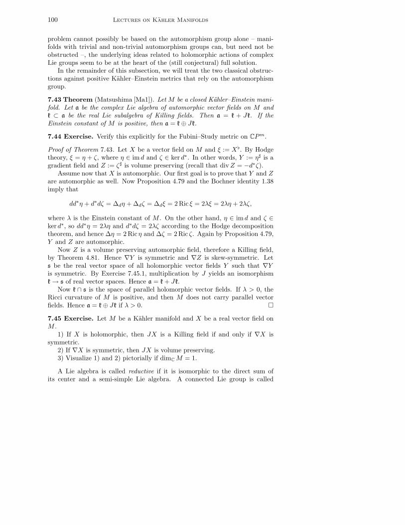
100 Lectures on Kahler Manifolds
problem cannot possibly be based on the automorphism group alone – mani-folds with trivial and non-trivial automorphism groups can, but need not beobstructed –, the underlying ideas related to holomorphic actions of complexLie groups seem to be at the heart of the (still conjectural) full solution.
In the remainder of this subsection, we will treat the two classical obstruc-tions against positive Kahler–Einstein metrics that rely on the automorphismgroup.
7.43 Theorem (Matsushima [Ma1]). Let M be a closed Kahler–Einstein mani-fold. Let a be the complex Lie algebra of automorphic vector fields on M andk ⊂ a be the real Lie subalgebra of Killing fields. Then a = k + Jk. If theEinstein constant of M is positive, then a = k⊕ Jk.
7.44 Exercise. Verify this explicitly for the Fubini–Study metric on CPm.
Proof of Theorem 7.43. Let X be a vector field on M and ξ := X. By Hodgetheory, ξ = η + ζ, where η ∈ im d and ζ ∈ ker d∗. In other words, Y := η♯ is agradient field and Z := ζ♯ is volume preserving (recall that divZ = −d∗ζ).
Assume now that X is automorphic. Our first goal is to prove that Y and Zare automorphic as well. Now Proposition 4.79 and the Bochner identity 1.38imply that
dd∗η + d∗dζ = ∆dη + ∆dζ = ∆dξ = 2 Ric ξ = 2λξ = 2λη + 2λζ,
where λ is the Einstein constant of M . On the other hand, η ∈ im d and ζ ∈ker d∗, so dd∗η = 2λη and d∗dζ = 2λζ according to the Hodge decompositiontheorem, and hence ∆η = 2 Ric η and ∆ζ = 2 Ric ζ. Again by Proposition 4.79,Y and Z are automorphic.
Now Z is a volume preserving automorphic field, therefore a Killing field,by Theorem 4.81. Hence ∇Y is symmetric and ∇Z is skew-symmetric. Lets be the real vector space of all holomorphic vector fields Y such that ∇Yis symmetric. By Exercise 7.45.1, multiplication by J yields an isomorphismk→ s of real vector spaces. Hence a = k + Jk.
Now k ∩ s is the space of parallel holomorphic vector fields. If λ > 0, theRicci curvature of M is positive, and then M does not carry parallel vectorfields. Hence a = k⊕ Jk if λ > 0.
7.45 Exercise. Let M be a Kahler manifold and X be a real vector field onM .
1) If X is holomorphic, then JX is a Killing field if and only if ∇X issymmetric.
2) If ∇X is symmetric, then JX is volume preserving.3) Visualize 1) and 2) pictorially if dimC M = 1.
A Lie algebra is called reductive if it is isomorphic to the direct sum ofits center and a semi-simple Lie algebra. A connected Lie group is called
7 Calabi Conjecture 101
reductive if its Lie algebra is reductive. We note the following consequence ofTheorem 7.43.
7.46 Corollary. If M is a closed Kahler–Einstein manifold, then the compo-nent of the identity of the automorphism group of M is reductive.
Proof. Let a and k be as above. Since k is the Lie algebra of a compact Liegroup, k = z ⊕ [k, k], where z is the center of k. Moreover, the commutatorsubalgebra [k, k] of k is semi-simple. Now k∩Jk consists of parallel vector fields,see Exercise 7.45.1, hence k ∩ Jk ⊂ z. Therefore
a = k + Jk = (z + Jz)⊕ ([k, k] + J [k, k]).
Since a = k+Jk, the center of a is z+Jz, and [k, k]+J [k, k] is semi-simple.
7.47 Example. Let M be the once blown up CP 2 as in Example 2.43. TheLie algebra a of the automorphism group of M consists of the matrices
0 ∗ ∗0 ∗ ∗0 ∗ ∗
∈ C
3×3.
The center of a is trivial. However, a is not semi-simple since the space ofmatrices in a with zero entries in second and third row is an Abelian ideal.Hence a is not reductive, and hence M does not carry Kahler–Einstein metrics.
By an analogous argument, the blow up of CP 2 in two points does not carrya Kahler–Einstein metric either; we leave this as an exercise. The blow up ofCP 2 in one or two points carries Kahler metrics with Ric > 0, see [Hit], [Ya1].Moreover, the blow up of CP 2 in one point carries Riemannian metrics withRic > 0 and sectional curvatures ≥ 0 [Che] and Einstein metrics with Ric > 0which are conformal to Kahler metrics [PP].
7.48 Remark. For closed Kahler manifolds of constant scalar curvature, westill have a = k+Jk, see [Li2]. Hence the argument in the proof of Corollary 7.46applies and shows that the identity components of the automorphism groupsof such manifolds are also reductive. In particular, the once and twice blownup CP 2 do not even admit Kahler metrics of constant scalar curvature.
We now discuss a second obstruction to the existence of positive Kahler–Einstein metrics which is also related to the automorphism group. Let M be aclosed Kahler manifold with Kahler form ω and Ricci form ρ.
7.49 Theorem (Futaki [Fu]). Assume that ω ∈ 2πc1(M) and write ρ − ω =
i∂∂Fω with Fω ∈ E(M,R). Then the map
Fω : a→ R, Fω(X) :=
∫
M
X(Fω)ωm,
does not depend on the choice of the Kahler form ω ∈ 2πc1(M).
102 Lectures on Kahler Manifolds
We remark that the function Fω in the definition of the map Fω exists, andis unique up to a constant, since ρ ∈ 2πc1(M) ∈ H1,1(M,R), see Exercise 5.51.
The map F = Fω, with ω ∈ 2πc1(M) an arbitrary Kahler form, is calledthe Futaki invariant of M . If ω is a Kahler–Einstein metric, ω = ρ, then Fω isconstant and the Futaki invariant Fω vanishes on a. The Futaki invariant ofboth the once and the twice blown up CP 2 is non-zero, see [Ti3, Section 3.2].Hence we conclude again that these two do not admit Kahler–Einstein metrics.
Let H1 → CP 1 and H2 → CP 2 be the hyperplane bundles. Let M be thetotal space M of the projective bundle of the product H1×H2 → CP 1×CP 2, aclosed and complex manifold of complex dimension 4. Futaki [Fu, §3] shows thatM is a Fano manifold with reductive automorphism group but non-zero Futakiinvariant. Hence the Matsushima criterion for the non-existence of Kahler–Einstein metrics does not apply in this case, whereas the Futaki obstructiondoes.
Proof of Theorem 7.49. We let ωt, −ε < t < ε, be a smooth family of Kahlerforms in 2πc1(M). The goal is to show that
∂t(Fωt
(X))
= 0.
By Exercise 5.51, ωt − ω0 = i∂∂Φt and ρt − ωt = i∂∂Ft for families of smoothfunctions Φt and Ft. From the proof of the ddc-Lemma 5.50 we see that thesefamilies of functions can be chosen to be smooth in t. As in (7.15), we compute
−i∂∂ lnM(Φt) = ρt − ρ0 = i∂∂(Ft + Φt − F0),
hence − lnM(Φt) = Ft + Φt − F0 + constant.
From now on, we mostly suppress the parameter t in our notation andindicate differentiation with respect to t by a dot or by ∂t. With ϕ = Φ andf = F we get ω = i∂∂ϕ and ρ− ω = i∂∂f . The displayed equation above gives
∆ϕ = 2f + 2ϕ,
compare Exercise 5.51. By Exercise 7.50, we have
2∂tωmt = 2mω ∧ ωm−1 = 2mi∂∂ϕ ∧ ωm−1 = −∆ϕ · ωm.
Thus
2∂t(Fωt
(X))
= 2
∫
M
(Xf)ωm + (XF )∂tωm
=
∫
M
X(∆ϕ− 2ϕ)− (XF )∆ϕ
ωm.
7 Calabi Conjecture 103
From now on, we suppress the measure of integration since it is always ωm.Because X is holomorphic,
∫
M
X(∆ϕ) =
∫
M
〈X, grad∆ϕ〉
=
∫
M
Ric(X, gradϕ) + 〈X,∇∗∇(gradϕ)〉
=
∫
M
Ric(X, gradϕ) + 〈∇∗∇X, gradϕ〉
= 2
∫
M
Ric(X, gradϕ),
by Exercise 6.17 and Proposition 4.79. It follows that∫
M
X(∆ϕ− 2ϕ) = 2
∫
M
Ric(X, gradϕ)− 〈X, gradϕ〉
= 2
∫
M
ρ(X, J gradϕ)− ω(X, J gradϕ)
= 2
∫
M
(i∂∂F )(X, J gradϕ)
=
∫
M
∇2F (gradϕ,X) +∇2F (J gradϕ, JX),
because of ρ− ω = i∂∂F and Exercise 7.50. Now
div((XF ) gradϕ) = 〈grad(XF ), gradϕ〉 − (XF )∆ϕ,
hence∫
M
(XF )∆ϕ =
∫
M
〈grad(XF ), gradϕ〉
=
∫
M
∇2F (gradϕ,X) + 〈∇gradϕX, gradF 〉
.
Since X is automorphic and J is parallel,
〈∇gradϕX, gradF 〉 = 〈∇J gradϕX, J gradF 〉 = −〈∇J gradϕJX, gradF 〉.
Adding up, we get
2∂t(Fωt
(X))
=
∫
M
∇2F (J gradϕ, JX) + 〈∇J gradϕJX, gradF 〉
=
∫
M
(J gradϕ)(JX(F )) = −∫
M
(JX(F )) div(J gradϕ).
Now div J gradϕ = 0, see Exercise 7.45.2, hence ∂t(Fωt
(X))
= 0.

104 Lectures on Kahler Manifolds
7.50 Exercise. Let M be a Kahler manifold and ϕ be a smooth function onM . Show that
2mi∂∂ϕ ∧ ωm−1 = −∆ϕ · ωm, (1)
2i∂∂ϕ(X, JY ) = ∇2ϕ(X,Y ) +∇2ϕ(JX, JY ). (2)
The complex Hessian of ϕ is defined by Hessc ϕ(X,Y ) = i∂∂ϕ(X, JY ). Writedown Hessϕ = ∇2ϕ and Hessc ϕ in Kahler normal coordinates.
7.51 Remark. Calabi generalized the Futaki invariant to general closed KahlermanifoldsM : Fix a Kahler metric ω onM and write ρω = γω+i∂∂Fω, where γωis the unique ω-harmonic form in 2πc1(M). Then the Calabi–Futaki invariant
CFω : a→ R, CFω(X) :=
∫
M
X(Fω)ωm, (7.52)
does not depend on the choice of ω in its Kahler class. It vanishes if theKahler class of ω contains a Kahler metric with constant scalar curvature. Thepreviously defined Futaki invariant is the special case where ω ∈ 2πc1(M) (if thelatter is positive definite). Our proof of Theorem 7.49 follows Futaki’s originalargument. For a discussion of the more general Calabi–Futaki invariant, seefor example Chapter 2.I in [Bes], Section 3.1 in [Ti3], or Section 1.6 in [Bo3].
It follows from work of Siu, Tian, and Yau that among the Fano surfacesas in Example 7.4.2, only the blow ups of CP 2 in one or two points do notadmit Kahler–Einstein metrics [Si2], [Ti1], [Ti2], [TY]. These are precisely theones whose automorphism group is not reductive and whose Futaki invariantsdo not vanish. In higher dimensions, the situation is much more complicated.There are examples, where the C0-estimates in the continuity method could beverified. For example, the Fermat hypersurfaces
zd0 + · · ·+ zdn = 0
in CPn carry Kahler–Einstein metrics if (n + 1)/2 ≤ d ≤ n, see [Na], [Si2],[Ti1] and compare Example 7.4.1. For surveys on Kahler–Einstein metrics, werefer to [Bo3] and [Ti3]. More recent references are [Bi] and [Th]. All thesereferences contain extensive bibliographies as well.
8 Kahler Hyperbolic Spaces
A question attributed to Chern asks whether the Euler characteristic of a closedRiemannian manifold M of dimension 2m satisfies
(−1)mχ(M) > 0 (8.1)
if the sectional curvature K of M is negative. The answer is yes if m ≤ 2, see[Chr] for the case m = 2. Dodziuk and Singer remarked that Atiyah’s L2-indextheorem implies (8.1) if the space of square integrable harmonic forms on theuniversal covering space of M vanishes in degree 6= m and does not vanish indegree = m. In [Gr], Gromov proves this and more in the case where M isa Kahler manifold; in this section we are concerned with his arguments andresults.
Let M be a complete and connected Riemannian manifold and E be a flatHermitian vector bundle over M . Choose an origin o ∈ M and let r = d(o, · )be the distance to o. Let α be a differential form on M with values in E andµ : R+ → R+ be a non-decreasing function. We say that α is O(µ(r)) if thereis a constant c such that
|α| ≤ cµ(cr + c) + c, (8.2)
where we consider the norm |α| = |α(p)| as a function onM . Following Gromov,we say that α is d(O(µ(r))) if there is a differential form β on M with α = dβand such that β is O(µ(r)). We also write d(bounded) instead of d(O(1)), thatis, in the case where β can be chosen to be uniformly bounded.
8.3 Examples. 1) Let M = Rn with Euclidean metric and origin 0. Let α bethe volume form of M , α = dx1 ∧ · · · ∧ dxn. Let β be an (n − 1)-form withdβ = α. Then on B = B(r, 0),
volnB =
∫
B
α =
∫
∂B
β ≤ max|β(p)| | p ∈ ∂B voln−1 ∂B.
It follows that
max|β(p)| | p ∈ ∂B ≥ volnB
voln−1 ∂B=r
n.
Hence α is not d(bounded). In a similar way one can treat each of the differ-ential forms dxI , where I is a multi-index.
2) Let α be a bounded 1-form on M and f be a smooth function withdf = α. Then
|df | = |α| ≤ ‖α‖∞ := sup|α(p)| | p ∈M.
Hence f is Lipschitz continuous with Lipschitz constant ‖α‖∞ if ‖α‖∞ <∞.
106 Lectures on Kahler Manifolds
8.4 Proposition. Let M be complete and simply connected and α be a differ-ential form on M of degree k with ‖α‖∞ <∞ and dα = 0.
1) If K ≤ 0, then α = d(O(r)).2) If K ≤ −c2 < 0 and k ≥ 2, then α = d(bounded).
Proof. Since M is complete and simply connected with non-positive sectionalcurvature, the theorem of Hadamard–Cartan implies that expo : ToM → M isa diffeomorphism. Hence we may define
τt(p) := expo(t exp−1o (p)),
where 0 ≤ t ≤ 1. Comparison with Euclidean space shows that the differentialof τt satisfies
|τt∗v| ≤ t|v|.The usual proof of the Poincare lemma provides a (k− 1)-form β with dβ = α.In Riemannian normal coordinates, β is given by
β(x) = r
∫ 1
0
tk−1(νxα)(tx) dt = r
∫ 1
0
τ∗t (νxα)(x) dt,
where r = |x| and ν is the radial normal field. By the above estimate
|τ∗t (νxα)| ≤ tk−1|νxα| ≤ tk−1‖α‖∞,
and hence
|β(p)| ≤ r
k‖α‖∞,
where p = exp(x). Note that this estimate is optimal, see Example 8.3.1 above.Suppose now that the sectional curvature of M is negative, K ≤ −c2 < 0.
Comparison with hyperbolic space shows that, for v perpendicular to ν,
|τt∗v| ≤sinh(ctr)
sinh(cr)|v|,
where r is the distance of the foot point of v to o. Hence
|β(p)| ≤ r∫ 1
0
( sinh(ctr)
sinh(cr)
)k−1dt · ‖α‖∞
=
∫ r
0
( sinh(cs)
sinh(cr)
)k−1ds · ‖α‖∞
≤∫ 0
−∞
(e(k−1)cs) ds · ‖α‖∞ =1
(k − 1)c‖α‖∞,
therefore α = d(bounded).
8 Kahler Hyperbolic Spaces 107
8.5 Remark. The estimates in the proof are explicit. Note also that the lift ofa differential form on a compact manifold to any covering manifold is uniformlybounded.
8.6 Proposition. Let (G,K) be a Riemannian symmetric pair such that M =G/K is a symmetric space of non-compact type. If α is a G-invariant differen-tial form on M , then α is parallel and hence closed. If α is of positive degree,then the restriction of α to maximal flats in M vanishes and α = d(bounded).
This result seems to be well known to experts, I learned it from AnnaWienhard. The proof (and even the statement) of Proposition 8.6 requiresmore on symmetric spaces than we develop in Appendix B. Therefore we onlygive a brief sketch of the argument. Good references for symmetric spaces ofnon-compact type are Chapter 2 in [Eb] and Chapter VI in [Hel].
Sketch of proof of Proposition 8.6. We can assume that (G,K) is an effectivepair. By Remark B.36, G contains the connected component of the identity ofthe isometry group of M . By Theorem B.24.3, α is parallel and hence closed.
Let F ⊂ M be a maximal flat and p ∈ F . There is a basis of TpF suchthat the reflections of TpF about the hyperplanes perpendicular to the vectorsof the basis are realized by the differentials of isometries g ∈ G fixing p. Sinceα is invariant under G, it follows easily that α|TpF = 0.
Let c : R → M be a regular unit speed geodesic and b : M → R be theBusemann function centered at c(∞) with b(c(t)) = −t. Let V = − grad b and(ft) be the flow of V . Then, for each p ∈ M , cp(t) = ft(p), t ∈ R, is the unitspeed geodesic through p asymptotic to c. In particular, cp is also regular and,therefore, contained in a unique maximal flat Fp. The flats Fp constitute asmooth foliation F of M by totally geodesic Euclidean spaces.
For any unit tangent vector u of M perpendicular to F , 〈R(u, V )V, u〉 isnegative and, by homogeneity, bounded away from 0 by a negative constantwhich does not depend on u. In particular, the Jacobi fields of geodesic vari-ations by geodesics cp and perpendicular to F decay uniformly exponentially.Since α vanishes along F , it follows easily that
γ = −∫ ∞
0
F ∗t αdt
is a well defined smooth differential form on M such that LV γ = α and dγ = 0.With β = V xγ we get
α = LV γ = d(V xγ) + V xdγ = dβ.
Now γ is uniformly bounded and |V | = 1, hence α = d(bounded).
8.7 Definition (Gromov). Let M be a Kahler manifold with Kahler formω. We say that M is Kahler-hyperbolic if the Kahler form ω of the universalcovering space M of M is d(bounded).
108 Lectures on Kahler Manifolds
Recall that the cohomology class of the Kahler form of a closed Kahler mani-fold M is non-trivial. Hence closed Kahler manifolds with finite fundamentalgroup are not Kahler-hyperbolic. On the other hand, if the sectional curvatureof M is strictly negative, then M is Kahler-hyperbolic, by Proposition 8.4. ByProposition 8.6, Hermitian symmetric spaces of non-compact type are Kahlerhyperbolic as well. These do not have strictly negative curvature if their rank,that is, the dimension of their maximal flats, is larger than 1.
Kahler-hyperbolic Kahler manifolds are the main topic in Gromov’s article[Gr]. Cao and Xavier [CX] and independently Jost and Zuo [JZ] observed thatthe arguments of Gromov concerned with the vanishing of square integrableharmonic forms work also under the weaker assumption that the Kahler formis d(O(µ)), where
∑∞1 1/µ(n) =∞. Note that this assumption is fulfilled if M
is simply connected with non-positive sectional curvature, by Proposition 8.4.1.We include this extension into our discussion, see Theorem 8.9 below.
For the rest of this section we assume that M is a complete and connectedKahler manifold with Kahler form ω and complex dimension m. We let E →Mbe a flat Hermitian vector bundle. Declaring parallel sections as holomorphicturns E into a holomorphic vector bundle such that the Chern connection ofthe given Hermitian metric is the given flat connection.
Without further notice we use notation and results from Appendix C. Wedo not assume throughout that differential forms are smooth and indicate theirregularity when appropriate.
8.1 Kahler Hyperbolicity and Spectrum. One of the remarkable proper-ties of Kahler manifolds is that the Lefschetz map commutes with the Laplacian:If α is a harmonic form with values in E, then ω ∧ α is harmonic as well. Thisis one of the cornerstones in the arguments which follow.
8.8 Lemma. Suppose that ω is d(O(µ(r))), where∑∞
1 1/µ(n) =∞. Let α bea closed and square integrable differential form with values in E. Then
d∗(ω ∧ α) = 0 =⇒ ω ∧ α = 0.
Proof. Choose an origin o ∈M , and let r : M → R be the distance to o. SinceM is complete and connected, the sublevels of r are relatively compact andexhaust M . Choose cut off functions ϕn : M → R, n ≥ 1, with ϕn(p) = 1 ifr(p) ≤ n, ϕn(p) = 0 if r(p) ≥ n+ 1 and |dϕn| ≤ c0.
Let ω = dη with |η| = O(µ(r)). Since dα = 0 = d∗(ω ∧ α) and ϕnη issmooth with compact support,
0 =
∫
M
(d∗(ω ∧ α), ϕnη ∧ α) =
∫
M
(ω ∧ α, d(ϕnη ∧ α))
=
∫
An
(ω ∧ α, dϕn ∧ η ∧ α) +
∫
M
(ω ∧ α, ϕnω ∧ α),
8 Kahler Hyperbolic Spaces 109
where An := p ∈ M | n ≤ r(p) ≤ n + 1 contains the support of dϕn. TheL2-norm of ω∧α is finite since ω is parallel and, therefore, uniformly bounded.Hence the second term on the right tends to the square of the L2-norm of ω∧αas n→∞. Now
∫
An
∣∣(ω ∧ α, dϕn ∧ η ∧ α)∣∣ ≤ (cµ(cn+ c) + c) · ‖ω‖∞
∫
An
|α|2.
Hence the assertion follows if the limes inferior of the sequence on the righthand side is 0. If the latter would not hold, then there would be an ε > 0 suchthat
‖α‖22 =
∫
M
|α|2 =∑
n
∫
An
|α|2 ≥∑ ε
(cµ(cn+ c) + c) · ‖ω‖∞=∞.
This would be in contradiction to the assumption that α is square integrable.
8.9 Vanishing Theorem (Cao–Xavier [CX], Jost–Zuo [JZ]). If ω is d(O(µ)),where
∑∞1 1/µ(n) =∞, then
Hk2(M,E) = 0 for k 6= dimC M.
Proof. For k < m this follows from Theorem C.49 and Lemma 8.8. For k > m,vanishing follows from Poincare duality.
8.10 Main Lemma. Suppose ω = dη with ‖η‖∞ <∞. Let α ∈ L2(Ak(M,E))be in the domain of ∆d,max and suppose that k 6= m or that α ⊥ Hm2 (M,E).Then
(∆d,maxα, α)2 ≥ λ2‖α‖22 with λ2 = c(m)/‖η‖2∞ > 0.
Proof. Assume first that k = m+ s > m. The s-th power of the Lefschetz mapdefines a parallel field of isomorphisms Am−s(M,E) → Am+s(M,E), see thediscussion in Section 5. In particular, there is β ∈ L2(Am−s(M,E)) such thatα = ωs ∧ β.
Since E is flat, ∆d = (d + d∗)2, hence ∆d,max = ∆d,min, by Theorem C.19.Hence we can assume that α and β are smooth with compact support. Let
θ := η ∧ ωs−1 ∧ β.
Thendθ = ωs ∧ β − η ∧ ωs−1 ∧ dβ =: α− α′.
Now |θ| ≤ |η||ωs−1||β|, hence
‖θ‖2 ≤ ‖η‖∞|ωs−1|‖β‖2,
where we note that |ωs−1| is constant. Since L±s is parallel, there is a positiveconstant c0 such that |Lsγ| ≤ c0|γ| for all γ ∈ Am−s(M,E) and |L−sγ| ≤ c0|γ|
110 Lectures on Kahler Manifolds
for all γ ∈ Am+s(M,E). Since Ls commutes with ∆d, we have Ls∆dβ = ∆dα,hence
‖dβ‖22 ≤ (∆dβ, β)2 ≤ ‖∆dβ‖2‖β‖2 ≤ c20‖∆dα‖2‖α‖2.We conclude that
‖α′‖2 ≤ c0‖η‖∞|ωs−1|‖∆dα‖1/22 ‖α‖1/22 .
We also have
(d∗α, θ)2 ≤ ‖d∗α‖2‖θ‖2 ≤ (∆dα, α)1/22 ‖θ‖2
≤ ‖η‖∞|ωs−1|‖∆dα‖1/22 ‖α‖1/22 ‖β‖2
≤ c0‖η‖∞|ωs−1|‖∆dα‖1/22 ‖α‖3/22 .
Therefore
‖α‖22 = (α, dθ + α′)2
= (α, dθ)2 + (α, α′)2
≤ (d∗α, θ)2 + ‖α‖2‖α′‖2≤ 2c0‖η‖∞|ωs−1|‖∆dα‖1/22 ‖α‖
3/22 .
Since ∆d,max is self-adjoint and non-negative, this proves the asserted inequalityin the case k > m. By applying Poincare duality we conclude that it also holdsin the case k < m.
We note that for a differential form α of pure degree, we have
α ∈ dom(d+ d∗)max iff α ∈ dom dmax ∩ dom d∗max.
Since (d+ d∗)max = (d+ d∗)min, the above inequality shows that, for k 6= m,
‖dmaxα‖22 + ‖d∗maxα‖22 ≥ λ2‖α‖22for any differential k-form α ∈ dom(d+ d∗)max. Now im d ⊂ dom dmax, hence
domdmax = dom dmax ∩ (ker d∗max + im d)
= dom dmax ∩ kerd∗max + im d.
Since im d ⊂ ker dmax, it follows that the image of dmax on differential forms ofdegree m− 1 is equal to the image of its restriction to
domdmax ∩ kerd∗max ∩ L2(Am−1(M,E)).
By the above estimate we have
‖dmaxα‖22 ≥ λ2‖α‖22
8 Kahler Hyperbolic Spaces 111
for any α in the latter space. In particular, the image of dmax on differentialforms of degree m− 1 is closed. Therefore it contains im d ∩ L2(Am(M,E)).
There is a similar discussion for d∗max on forms of degree m+ 1. Hence wecan represent any γ ∈ dom∆d,max∩L2(Am(M,E)) perpendicular to Hm2 (M,E)as
γ = dmaxα+ d∗maxβ,
where dmaxα ∈ im d ⊥ im d∗ ∋ d∗maxβ and
d∗maxα = dmaxβ = 0, ‖dmaxα‖2 ≥ λ2‖α‖2, ‖d∗maxβ‖2 ≥ λ2‖β‖2.
We have
γ ∈ dom∆d,max = dom∆d,min ⊂ dom(d+ d∗)min = dom(d+ d∗)max.
Considering degrees, we get
dmaxα ∈ domd∗max, d∗maxβ ∈ domdmax,
and hence α, β ∈ dom∆d,max. In conclusion,
‖γ‖22 = ‖dmaxα‖22 + ‖d∗maxβ‖22= (∆d,maxα, α)2 + (∆d,maxβ, β)2
≤ ‖∆d,maxα‖2‖α‖2 + ‖∆d,maxβ‖2‖β‖2≤ λ−2 · (‖∆d,maxα‖22 + ‖∆d,maxβ‖22)= λ−2 · (‖d∗maxγ‖22 + ‖dmaxγ‖22) = λ−2 · (∆γ, γ)2.
Let E′, E′′ →M be Hermitian vector bundles overM andD be a differentialoperator of first order from E(E′) to E(E′′). Let F →M be a further Hermitianvector bundle with Hermitian connection ∇21. Define
SF : E′ ⊗ T ∗M ⊗ F → E′′ ⊗ F, SF (α⊗ dϕ⊗ σ) = (S(dϕ)α) ⊗ σ, (8.11)
where S is the principal symbol of D, see (C.10). The twist of D by ∇ is thedifferential operator D∇ : E(E′ ⊗ F )→ E(E′′ ⊗ F ) defined by
D∇(α⊗ σ) = (Dα)⊗ σ + SF (α⊗∇σ). (8.12)
8.13 Example. For D = d+ d∗, we have
SF (α ⊗∇σ) :=∑(X
j ∧ α) ⊗∇Xjσ − (Xjxα)⊗∇Xj
σ,
where (Xj) is a local orthonormal frame of TM .
21We are short of symbols since D is in use already.
112 Lectures on Kahler Manifolds
If ∇, ∇0 are Hermitian connections on F and A = ∇−∇0, then
(D∇ −D∇0
)(α⊗ σ) = SF (α⊗Aσ) =: SA(α⊗ σ) (8.14)
is of order 0, a potential perturbing D∇0
. We apply this in the case whereF = M × C is the trivial line bundle over M with the canonical Hermitianmetric and canonical flat and Hermitian connection ∇0. Let ζ be a real valueddifferential one-form on M . Then
∇ = ∇0 +A, (8.15)
whereAσ := iζ ⊗ σ, (8.16)
is a connection form for F . Since iζ is purely imaginary, ∇ is Hermitian. Thecurvature form of ∇ is idζ. Vice versa, if ∇ is a Hermitian connection on aHermitian line bundle F →M and the curvature form of ∇ is exact, say equalto idζ, then ∇0 = ∇− iζ ⊗ id is a flat Hermitian connection (and F is trivialif M is simply connected).
8.17 Lemma. Suppose ω = dη with ‖η‖∞ <∞. Let D = ∂+∂∗ on A∗(M,E)and λ be as in Lemma 8.10. Let F = M × C be the trivial line bundle over Mwith ∇0 and ∇ = ∇0 + iζ ⊗ id as above. Assume that |SAβ| ≤ c · |β| for somepositive constant c < λ/
√2. Then
kerDmax = 0 =⇒ kerD∇max = 0.
Proof. Assume that kerDmax = 0. Since ∇0 is flat, we have
‖D∇0
β‖22 = (∆∂β, β)2 =
1
2(∆dβ, β)2 ≥
λ2
2‖β‖22
for all β ∈ A∗c(M,E ⊗ F ), by Lemma 8.10. Hence, for all such β,
‖D∇β‖2 = ‖D∇0
β + SAβ‖2≥ ‖D∇0
β‖2 − ‖SAβ‖2 ≥ (λ/√
2− c)‖β‖2.
Now D∇min = D∇
max, see Theorem C.19. Hence kerD∇max = 0 as asserted.
8.2 Non-Vanishing of Cohomology. We start with a little detour (and acorresponding change in notation) and discuss Atiyah’s L2-index theorem [At].Let M →M be a normal Riemannian covering, where M and M are connectedand M is closed. Let E → M be the pull back of a Hermitian vector bundleE →M . Then the group Γ of covering transformations of M →M acts on E,hence on sections of E by γ · σ := γ σ γ−1.
8 Kahler Hyperbolic Spaces 113
Let H ⊂ L2(M, E) be a closed subspace and (Φn) be an orthonormal basisof H . Then the function
f : M → [0,∞], f(p) =∑|Φn(p)|2, (8.18)
does not depend on the choice of (Φn). It follows that f is Γ-invariant if H is,and then f is the lift of a function f on M and we set
dimΓH =
∫
M
f, (8.19)
the Γ-dimension of H . It is important that dimΓH 6= 0 iff H 6= 0.Let E± → M be Hermitian vector bundles and D : E(E+) → E(E−) be a
differential operator. Let E± and D be the pull backs of E± and D to M .Then the kernels of D and its formal adjoint D∗ are Γ-invariant. By definition,the Γ-index of D is
indΓ D = dimΓ ker D − dimΓ ker D∗. (8.20)
The Γ-index of D is well-defined if one of the dimensions on the right is finite.
8.21 Theorem (Atiyah [At]). If D is elliptic, then the Γ-dimensions on theright hand side of (8.20) are finite and
indΓ D = indD.
Theorem 8.21 applies in the case of non-positively curved closed Kahlermanifolds and shows that their Euler characteristic has the right sign. Moreprecisely, we have the following result.
8.22 Theorem (Cao–Xavier [CX], Jost–Zuo [JZ]). Let M be a closed Kahlermanifold and M → M be its universal cover. If the Kahler form ω of M isd(O(µ)), where
∑∞1 1/µ(n) =∞, then
(−1)mχ(M,E) ≥ 0.
Proof. By Hodge theory, χ(M,E) = indD, whereD = d+d∗ fromAeven(M,E)to Aodd(M,E). We have D = d+d∗, but now fromAeven(M, E) to Aodd(M, E).By Theorem 8.21, indD = indΓ D, where Γ is the fundamental group of M .By Theorem 8.9, there are no non-trivial square integrable harmonic forms onM of degree different from the middle dimension. Hence
(−1)m indΓ D = dimΓHm(M,E) ≥ 0.
Gromov uses an extended version of (part of) Theorem 8.21. He considersthe twist of the pull back of a specific bundle E with the trivial complex line
114 Lectures on Kahler Manifolds
bundle endowed with a Hermitian connection ∇ which is not invariant underΓ, whereas the curvature of ∇ still is.
For the reader’s convenience, but without proof, we state a more generalversion of Gromov’s extension. Let E → M be a Hermitian vector bundle ofrank r, not necessarily the pull back of a Hermitian vector bundle over M . LetG be an extension of Γ by a compact group K,
1 −→ K −→ Gρ−→ Γ −→ 1. (8.23)
Suppose that G acts by Hermitian isomorphisms on E such that
π g = ρ(g) π for all g ∈ G, (8.24)
where π denotes the projection of E. Then G acts on L2(M, E) by
g · σ := g σ ρ(g)−1. (8.25)
Let H be a G-invariant subspace of L2(M, E). Then the function f as in(8.18) is Γ-invariant, and we define the G-dimension of H by the integral of thecorresponding function f on M as in (8.19).
Let E± be Hermitian vector bundles with Hermitian G-actions satisfying(8.24) (where now π denotes the projections of E±). Suppose that D is adifferential operator from E(E+) to E(E−) commuting with the actions of G,
D(g · σ) = g · (Dσ). (8.26)
Then the kernels of D and D∗ are invariant under G, and we define the G-indexof D as in (8.20). The case considered in Theorem 8.21 corresponds to thetrivial extension G = Γ. The extension we state concerns the case where E =E+ ⊕ E− is a graded Dirac bundle and D+ : E(E+) → E(E−) the associatedDirac operator in the sense of Gromov and Lawson, see Subsection C.24.
8.27 Theorem. Suppose that E is a graded Dirac bundle and that the Hermi-tian action of G on E satisfies (8.24) and leaves invariant connection, Cliffordmultiplication, and splitting E = E+ ⊕ E− of E. Then the associated Dirac
operator D satisfies (8.26), the G-dimensions of ker D+ and ker D− are finite,the canonical index form α of D+ is the pull back of a form α on M , and
indG(D+) =
∫
M
α.
About the proof. It seems that the arguments in Section 13 of [Ro] generalizeto the setting of Theorem 8.27.
8.28 Remark. We will need Theorem 8.27 for the Hirzebruch–Riemann–Rochformula, that is, for the twisted Dolbeault operator ∂ + ∂∗ (times
√2) on the
Dirac bundle
Ap,∗(M, E) = A0,∗(M,C)⊗Ap,0(M,C)⊗ E,
8 Kahler Hyperbolic Spaces 115
with splitting into forms with ∗ even and odd, respectively, see Example C.27.2.In this case, the canonical index form is
Td(M) ∧ ch(Ap,0(M,C)⊗ E) = Td(M) ∧ ch(Ap,0(M,C)) ∧ ch(E),
where Td and ch denote Todd genus and Chern character, see Theorem III.13.15in [LM].
Before returning to the discussion of Kahler manifolds, we discuss a situationwhere a group G as above arises in a natural way. To that end, suppose inaddition that M is simply connected. Let F → M be a Hermitian line bundlewith Hermitian connection∇ such that the curvature form ω of∇ is Γ-invariant.
8.29 Lemma. Let p ∈ M , γ ∈ Γ, and u : Fp → Fγp be a unitary map. Thenthere is a unique lift of γ to an isomorphism g of F over γ with gp = u andsuch that g preserves Hermitian metric and connection of F .
Sketch of proof. Let q ∈ M and y ∈ Fq. Choose a piecewise smooth path cin M from p to q. Let x be the element in Fp which is parallel to y along c.Set g(y) = z, where z is parallel to ux along γ c. The dependence of paralleltranslation on curvature together with the Γ-invariance of ω shows that z onlydepends on the homotopy class of c. Since M is simply connected, g is welldefined. By definition, u preserves parallel translation, hence ∇. Since ∇ isHermitian, g preserves the Hermitian metric of F .
It follows from Lemma 8.29 that there is an extension
1→ U(1)→ G→ Γ→ 1 (8.30)
of Γ by U(1) which lifts the action of Γ on M to an action of G on F as in(8.24). Furthermore, the action of G preserves metric and connection of F .
We now return to the discussion of Kahler-hyperbolic Kahler manifolds. Welet M be a closed and connected Kahler manifold and E →M be a flat vectorbundle. We let M → M be the universal covering of M and E → M be thepull back of E.
8.31 Main Theorem. If ω = dη with ‖η‖∞ <∞, then
Hp,q2 (M, E) 6= 0 if p+ q = m.
Proof. Let F = M × C be the trivial line bundle with canonical Hermitianmetric and flat connection ∇0, and consider the Hermitian connections
∇t = ∇0 + itη.
The curvature form of ∇t is itdη = itω, where ω denotes the Kahler form ofM with respect to the induced Kahler metric. Since ω is Γ-invariant, we get
116 Lectures on Kahler Manifolds
extensions Gt of Γ by U(1) with induced actions on F as in Lemma 8.29 above.
For each fixed t, consider the twist D∇t
of the Dolbeault operator D = ∂ + ∂∗
on Ap,∗(M, E) by F with connection ∇t. With respect to the splitting into
forms with ∗ even and odd, the index form of (D∇t
)+ is
Td(M) ∧ ch(Ap,0(M,C)) ∧ ch(E) ∧ ch(F ),
where chF = exp(−tω/2π), see (A.44) and Remark 8.28 above. Hence theindex form is a power series in t, where the coefficient of tm in degree dimR Mis
rkE
m!(−2π)m
(m
p
)· ωm.
By Theorem 8.27, the index indGt((D∇t
)+) is the integral of the index form
overM . It follows that indGt((D∇t
)+) is a polynomial in t, where the coefficientof tm is non-zero22. Hence the zeros of this polynomial are isolated.
On the other hand, Hp,q2 (M, E) = 0 would imply that indGt(D∇t
) = 0 forall t sufficiently small, by Lemma 8.17.
8.32 Theorem. If ω = dη with ‖η‖∞ <∞, then
(−1)mχ(M) =∑
p+q=m
dimΓHp,q2 (M, E) > 0,
where Γ denotes the fundamental group of M .
Proof. This is immediate from Theorems 8.21, 8.9, and 8.31, compare the proofof Theorem 8.22.
22This is in contrast to the case of compact manifolds, where the index of elliptic differentialoperators is integral and would not depend on t.
9 Kodaira Embedding Theorem
Let M be a closed complex manifold of complex dimension m. Recall that aholomorphic line bundle E → M is positive or negative if its first Chern classc1(E) has a positive or negative representative, respectively, see Definition 5.59.It is immediate that a holomorphic line bundle is positive iff its dual is negative.In Examples 5.60 we showed that the tautological bundle U → CPm is negativeand that the hyperplane bundle H → CPm is positive.
If M admits a positive holomorphic line bundle, then a positive representa-tive of its first Chern class is a Kahler metric on M . In this sense the topic ofthis section belongs to Kahler geometry.
9.1 Remark. We say that a cohomology class in H2(M,C) is integral if it is inthe image of the canonical morphism H2(M,Z)→ H2(M,C). If M is a Kahlermanifold, then a cohomology class in H2(M,C) is the first Chern class of aholomorphic line bundle iff it is of type (1, 1) and integral, see e.g. PropositionIII.4.6 in [Wel]. It follows that a closed complex manifold M admits a positiveholomorphic line bundle iff M has a Kahler metric g with integral Kahler class[ω]. Then M is called a Hodge manifold.
Closed oriented surfaces are Hodge manifolds: Let S be such a surface andg be a Riemannian metric on S. Then the rotation by a positive right angle, inthe tangent spaces of S, is a parallel complex structure on S and turns S intoa Kahler manifold. Since S is of real dimension two, H2(S,R) ∼= R. Now theimage of H2(S,Z) in H2(S,R) is a lattice, hence a proper rescaling of g has anintegral Kahler class. Hence S is a Hodge manifold. By the latter argument wealso get that a closed Kahler manifold M with first Betti number b1(M) = 1 isa Hodge manifold.
The pull back of a positive holomorphic line bundle along a holomorphicimmersion is positive. In particular, if M admits a holomorphic immersion intoCPn for some n ≥ m, then M admits a positive holomorphic line bundle. Viceversa, Hodge conjectured and Kodaira proved that M admits a holomorphicembedding into CPn for some n ≥ m if M has a positive line bundle. Wepresent Kodaira’s proof of his embedding theorem; our source is Section VI.4in [Wel].
Kodaira’s proof uses the following general construction which associates toa holomorphic line bundle E → M a holomorphic map from an open part M ′
of M to a complex projective space: Let O(M,E) be the space of holomorphicsections of E and M ′ be the open set of points p ∈ M such that σ(p) 6= 0for some σ ∈ O(M,E). Since M is compact, O(M,E) is of finite dimension.Consider the evaluation map
ε : E∗ → O(M,E)∗, ε(ϕ)(σ) = ϕ(σ(p)), (9.2)
where p is the foot point of ϕ. Clearly ε is holomorphic. For ϕ ∈ E∗ non-zero,
118 Lectures on Kahler Manifolds
ε(ϕ) 6= 0 precisely for p ∈M ′. Hence we obtain a holomorphic map
k : M ′ → P (O(M,E)∗), k(p) = [ε(ϕ)], (9.3)
where ϕ is any non-zero element of the fiber of E∗ over p.There is a somewhat less abstract way of describing k. Let B = (σ0, . . . , σk)
be a basis of O(M,E) and ϕ be a nowhere vanishing holomorphic section ofE∗ over an open subset U of M . Then the holomorphic map
kB : U → CP k, kB(p) = [ϕ σ0, . . . , ϕ σk], (9.4)
does not depend on the choice of ϕ. Hence kB is well defined on M ′. It is clearthat kB corresponds to k in the coordinates of O(M,E)∗ defined by the basisB.
We say that a holomorphic line bundle E → M is very ample if, in theabove construction, M ′ = M and k (or kB) is an embedding. We say that Eis ample if some positive power of E is very ample.
9.5 Exercise. Show that E∗ is isomorphic to the pull back under k of the tau-tological bundle over P (O(M,E)∗). Conclude that ample bundles are positive.
Kodaira proves the following more precise version of the embedding theo-rem.
9.6 Kodaira Embedding Theorem. Let M be a closed complex manifoldand E →M be a holomorphic line bundle. If E is positive, then E is ample.
Let E be a holomorphic line bundle over M and p be a point in M . Letϕ : U → E∗ be a nowhere vanishing holomorphic section of E∗, where U is anopen subset of M containing p. Then the 1-jet of a smooth section σ of E atp with respect to ϕ is
J1ϕ,p(σ) := ((ϕ σ)(p), (ϕ σ)′(p)) ∈ C⊕ (T ∗
pM ⊗ C), (9.7)
where (ϕσ)′ denotes the derivative of ϕσ. The proof that positive holomor-phic line bundles are ample relies on the following lemma.
9.8 Lemma. Let E be a line bundle over M . Suppose that1) for any two different points p, q ∈M , the map
J0p,q : O(M,E)→ Ep ⊕ Eq, J0
p,q(σ) = (σ(p), σ(q)),
is surjective and that2) for any point p ∈M and section ϕ about p as above, the map
J1ϕ,p : O(M,E)→ C⊕ (T ∗
pM ⊗ C)
is surjective. Then E is very ample.
9 Kodaira Embedding Theorem 119
Proof. We first observe that M ′ = M , by Assumption 1). For a basis B =(σ0, . . . , σk) of O(M,E), we consider kB : M → CP k as above.
Let p, q be different points of M . By Assumption 1), there are global holo-morphic sections σp and σq of E with
σp(p) 6= 0, σp(q) = 0 and σq(q) 6= 0, σq(p) = 0.
Then σp and σq are linearly independent. If we choose B with σ0 = σp andσ1 = σq , then clearly kB(p) 6= kB(q). It follows that kB is injective, for anychoice of basis B.
Let p be a point in M and ϕ be a holomorphic section of E∗ in an openneighborhood U of p as above. By Assumption 2), there are holomorphicsections σ0, . . . , σm in O(M,E) such that J1
ϕ,p(σ0) = (1, 0) and J1ϕ,p(σi) =
(0, βi), where (β1, . . . , βm) is a basis of T ∗pM ⊗ C. Since J1
ϕ,p is a linear map,σ0, . . . , σm are linearly independent in O(M,E). Therefore we can completethem to a basis B of O(M,E). With respect to affine coordinates (z1, . . . , zk)on z0 6= 0 ⊂ CP k, we get
dkB(p) = ((β1, . . . , βm, (ϕ σm+1)′(p), . . . , (ϕ σk)′(p)).
Since (β1, . . . , βm) are linearly independent, dkB(p) has rank m. Hence kB isan immersion. Now M is compact, hence kB is an embedding.
9.1 Proof of the Embedding Theorem. We use notation and results fromSubsection 3.4, in particular Examples 3.45 and Lemmas 3.46 and 3.47. Wedenote the blow up of M in a point p by Mp and use an index p for objectsassociated to Mp. For points p 6= q in M , we let Mpq = (Mp)q and πpq : Mpq →M be the canonical projection. There is a natural identification of Mpq withMqp such that πpq = πqp. We let Lpq be the holomorphic line bundle associatedto the hypersurface π−1
pq (p) ∪ π−1pq (q).
9.9 Lemma. Let E,F be holomorphic line bundles over M and suppose E > 0.Then given k0 ≥ 1 there is n0 ≥ 0 such that
π∗pE
n ⊗ π∗pF ⊗ (L∗
p)k > 0 and π∗
pqEn ⊗ π∗
pqF ⊗ (L∗pq)
k > 0
for all p 6= q ∈M , n ≥ n0, and k ∈ 1, . . . , k0.
Proof. Choose a Hermitian metric on E such that the curvature of its Chernconnection satisfies iΘE > 0, see Lemma 5.61. Fix a Hermitian metric on Fand denote the curvature of its Chern connection by ΘF . The Chern connectionof the tensor product E1 ⊗ E2 of two Hermitian holomorphic vector bundlesE1, E2 →M with induced Hermitian metric
(e1 ⊗ e2, e′1 ⊗ e′2) = (e1, e′1) (e2, e
′2)
120 Lectures on Kahler Manifolds
is given by the usual product rule, hence its curvature is the sum of the cur-vatures of the Chern connections on E1 and E2, Θ = Θ1 + Θ2. Since M iscompact and iΘE > 0, there is an n0 > 0 such that i(n0ΘE + ΘF ) > 0. Inparticular, En ⊗ F > 0 for all n ≥ n0.
Let p ∈M and consider the projection πp : Mp →M . The Chern connectionof the pull back of a Hermitian metric on the pull back of a holomorphic vectorbundle is the pull back of the Chern connection of the original Hermitian metricon the original bundle. Hence the Chern connection of the pull back metricon π∗
pEn ⊗ π∗
pF has curvature Θn equal to the pull back of the curvature onEn⊗F . Therefore iΘn(v, Jv) > 0 for v not in the kernel of πp∗, that is, exceptfor v = 0 or v tangent to Sp.
Positive powers of L∗p will bring positivity everywhere. To get n0 indepen-
dent of the chosen point p ∈ M , we proceed as follows: Choose holomorphiccoordinates z : U → U ′ on M , where U ′ contains the ball of radius 4 about 0in Cm. Set
Ui = p ∈ U | |z(p)| < i.Fix a cut off function χ on M with χ = 1 on U2 and χ = 0 on M \ U3.
For p in the closure U1 of U1, we use z − z(p) as holomorphic coordinatesin the construction of the blow up Mp. Via the canonical projection πp, we
identify Mp \ π−1p (U1) with M \ U1. In this sense, we view L∗
p restricted to
Mp \ π−1p (U1) as a holomorphic line bundle over M \ U1. The holomorphic
section Φ∗0 dual to the holomorphic section Φ0 as in Example 3.45.4 turns it
into a trivial bundle. We define a Hermitian metric h′p on this part of L∗p
by associating length 1 to Φ∗0. Then Φ∗
0 is parallel with respect to the Chernconnection of h′p, and hence the curvature of the latter vanishes identically.
Since the hyperplane bundle H → CPm−1 is positive, there is a Hermitianmetric h on H such that the curvature of its Chern connection satisfies iΘh >0. Over π−1
p (U4), we have L∗p = σ∗
pH , where σp : π−1p (U4) → CPm−1 is the
canonical projection. Therefore we view h′′p = σ∗ph as a Hermitian metric on
that part of L∗p. The curvature Θ′′
p of the Chern connection of h′′p is the pullback of Θh, and hence iΘ′′
p ≥ 0 and iΘ′′p > 0 on the tangent bundle of Sp. We
now lethp = (χ πp)h′′p + (1− χ πp)h′p.
Then the curvature Θp of the Chern connection of hp vanishes on Mp \π−1p (U3)
and Θp = Θ′′p on π−1(U2). Since σp(q) is smooth in p ∈ U1 and q ∈ U3 \ U2,
the family of Hermitian metrics h′′p , p ∈ U1, is uniformly bounded on U3 \ U2,together with derivatives of any order. It follows that Θp is uniformly bounded
on U3 \ U2, independently of p ∈ U1.The curvature of the Chern connection of the induced Hermitian metric on
En ⊗F ⊗ (L∗)k is Θ = Θn + kΘp. Clearly iΘ is positive outside U3 \U2. If weincrease the above n0 if necessary, the positivity of iΘn outweighs the possiblenegativity of kiΘp on U3 \ U2. By the uniform boundedness of Θp, n0 can be
9 Kodaira Embedding Theorem 121
chosen independently of p ∈ U1. Now M is compact, hence can be covered bya finite number of sets U1 as in the argument.
The argument in the case of two points p 6= q in a set U1 as above is similar.We use the same construction, but now with two pull backs of H correspondingto the two points p and q. For p and q uniformly far apart, we can apply theargument for the case of one point twice.
We now come to the final steps of the proof of the embedding theorem. Wewill assume some elementary facts from sheaf theory. For a sheaf F over Mand an open subset U of M , we denote by F(U) the space of sections of F overU . For p ∈M , we denote by Fp the stalk of F at p.
Let O be the structure sheaf of M , that is, the sheaf of rings of germs ofholomorphic functions on M . For p ∈M , let p and 2
p be the subsheaves ofideals in O of germs of holomorphic functions which vanish at p respectivelyvanish at p at least of second order. Then we have a short exact sequence
0→2p → O → O/2
p → 0. (9.10)
For q 6= p, the stalk (O/2p)q = 0. Moreover, the map
J1p : Op → C⊕ (T ∗
pM ⊗ C), J1p (f) = (f(p), f ′(p)), (9.11)
induces an isomorphism
(O/2p)p → C⊕ (T ∗
pM ⊗ C). (9.12)
Let F →M be a holomorphic line bundle. Denote by O(F ) the sheaf of germsof holomorphic sections of F . Since O(F ) is a locally free sheaf of modules overthe structure sheaf O of M , we obtain an induced short exact sequence
0→ O(F ) ⊗2p → O(F )→ O(F )⊗ (O/2
p)→ 0, (9.13)
where the tensor product is taken over O. We may view O(F ) ⊗2p as sheaf
of germs of holomorphic sections of F which vanish at least of second order atthe distinguished point p. The stalks in q 6= p are
(O(F ) ⊗2p)q = O(F )q and (O(F )⊗ (O/2
p))q = 0. (9.14)
To identify the stalk of O(F ) ⊗ (O/2p) at p, we observe that the map J1
ϕ,p
from Lemma 9.8 is also defined on the stalk O(F )p and that it induces anisomorphism
(O(F ) ⊗ (O/2p))p → C⊕ (T ∗
pM ⊗ C). (9.15)
9.16 Lemma. Let E →M be a positive holomorphic line bundle. In Lemma 9.9,let F be the canonical bundle of M , F = K, and k0 = m+1. Then En, n ≥ n0,satisfies the assumptions of Lemma 9.8 and hence E is ample.
122 Lectures on Kahler Manifolds
Proof. The proof of Assumption 1) in Lemma 9.8 is similar to and easier thanthe proof of Assumption 2). Therefore we concentrate on Assumption 2) andleave the proof of Assumption 1) to the reader.
Let p ∈ M . By (9.14), the restriction map induces an isomorphism fromthe space H0(M,O(En)⊗ (O/2
p)) of global holomorphic sections of O(En)⊗(O/2
p) onto the stalk (O(En)⊗ (O/2p))p. Hence it remains to show that
O(M,En) = H0(M,O(En))→ H0(M,O(En)⊗ (O/2p)) (9.17)
is surjective, by (9.15). Since points in M have codimension m and do notcorrespond to line bundles if m > 1, we will need to pass to blow ups of M toshow the surjectivity in (9.17).
Let M = Mp be the blow up of M in p. Let π : M → M be the canonical
projection and E = π∗E. Denote by O the structure sheaf of M and by Sand 2
S the subsheaves of O of germs of holomorphic functions which vanishalong S respectively vanish at least of second order along S. Composition withπ induces injective morphisms π∗ : O → O and π∗
µ : O(En)→ O(En). Now En
is trivial in a neighborhood of p in M , and the pull back of a local trivializationdefines a trivialization of En in a neighborhood of S. From the coordinatedescription of M in Subsection 2.4 it is then clear that a holomorphic section σof En vanishes of at least second order at p iff σ π vanishes of at least secondorder about S. It follows that π induces morphisms
π∗λ : O(En)⊗2
p → O(En)⊗2S
and
π∗ρ : O(En)⊗ (O/2
p)→ O(En)⊗ (O/2S).
Hence we get a commutative diagram
0 −−−−→ O(En)⊗2S −−−−→ O(En) −−−−→ O(En)⊗ O/2
S −−−−→ 0xπ∗
λ
xπ∗
µ
xπ∗
ρ
0 −−−−→ O(En)⊗2p −−−−→ O(En) −−−−→ O(En)⊗O/2
p −−−−→ 0(9.18)
of short exact sequences of sheaves.Clearly π∗
λ and π∗µ are injective. We claim that they are also surjective. This
is clear in the casem = 1 since then blowing up is trivial and π is biholomorphic.For m > 1, a section σ of En over M restricts to a section σp of En over M \S =M\p. By Hartogs’ theorem [GH, page 7], σp extends to a holomorphic sectionσ of En over M . By the continuity of σ and σ, we have π∗
µσ = σ. Moreover, ifσ vanishes of order at least 2 along S, then also σ at p. Hence π∗
λ and π∗µ are
surjective, hence isomorphic. The five lemma implies that π∗ρ is an isomorphism
as well.
9 Kodaira Embedding Theorem 123
A fortiori, the vertical morphisms in (9.18) induce isomorphisms betweenthe corresponding cohomology groups in the long exact sequences associated tothe horizontal short exact sequences. Thus by (9.17), it remains to show that
H0(M,O(En))→ H0(M,O(En)⊗ (O/2S))
is surjective. By the long exact sequence, this follows if H1(M,O(En)⊗2S) =
0.To show this we observe first that S = O(L∗). In the notation of Exam-
ple 3.45.4, this follows in Wi, i ≥ 1, since there f ∈ S can be expressed asf = fizi with fi holomorphic. That is, the functions zi serve as a frame overWi and fizi = f = fjzj over Wi ∩Wj . Now En ⊗ K∗ ⊗ (L∗)2 > 0 by Lemmas3.46 and 3.47, hence
H1(M,O(En ⊗ (L∗)2)) = 0
by the Kodaira vanishing theorem 5.65.
9.2 Two Applications. The Kodaira embedding theorem has many appli-cations. We discuss two immediate ones.
9.19 Corollary. Let M be a closed complex manifold and Mp be the blow upof M in a point p ∈M . If M admits a holomorphic embedding into a complexprojective space, then Mp as well.
Proof. Suppose f : M → CPn is a holomorphic embedding. Then the pull backE → M of the hyperplane bundle H over CPn is positive. By Lemma 9.9,π∗pE ⊗ (L∗)k is positive for k sufficiently large, where πp : Mp → M is the
natural map. Hence Mp admits a holomorphic embedding into some complexprojective space, by Theorem 9.6.
9.20 Corollary. Let M be a closed complex manifold and M →M be a finitecovering of M . If M admits a holomorphic embedding into a complex projectivespace, then M as well.
Proof. Suppose f : M → CPn is a holomorphic embedding. Then the pullback E → M of the hyperplane bundle H over CPn is positive, therefore thepull back E → M of E is positive as well. Hence M admits a holomorphicembedding into some complex projective space, by Theorem 9.6.
9.21 Remark. For a finite covering M → M as above, averaging leads tothe converse assertion: If M admits a holomorphic embedding into a complexprojective space, then also M , see [GH, page 192].
To complete the picture, we quote the theorem of Chow which says thata complex analytic submanifold of a complex projective space is a smoothprojective variety, see for example [GH, page 167].
Appendix A Chern–Weil Theory
In this appendix, no Kahler classes are in the way and, therefore, connectionand curvature forms are denoted by the more standard ω and Ω, respectively.
Let V1, . . . , Vk and V be vector spaces over the field F ∈ R,C and
Φ: V1 × · · · × Vk → V (A.1)
be a k-linear map. Let Λ∗FRn be the algebra of alternating forms on Rn with
values in F. The map
(ϕ1, v1, . . . , ϕk, vk) 7→ (ϕ1 ∧ · · · ∧ ϕk)⊗ Φ(v1, . . . , vk), (A.2)
where ϕi ∈ Λ∗FRn and vi ∈ Vi, is linear in each of its 2k arguments. Therefore
it gives rise to a k-linear map
ΦΛ : (Λ∗FR
n ⊗ V1)× · · · × (Λ∗FR
n ⊗ Vk)→ Λ∗FR
n ⊗ V. (A.3)
We view Λ∗FRn ⊗ Vi and Λ∗
FRn ⊗ V as the space of alternating forms on Rn
with values in Vi and V , respectively. If α1, . . . , αk are alternating forms on Rn
with values in V1, . . . , Vk and degrees d1, . . . , dk, respectively, and if we expressαi =
∑ϕij ⊗ vij with ϕij ∈ Λ∗
FRn and vij ∈ Vi, then
ΦΛ(α1, . . . , αk) =∑
(j1,...,jk)
(ϕ1j1 ∧ · · · ∧ ϕkjk )⊗ Φ(v1j1 , . . . , vkjk ). (A.4)
The degree of ΦΛ(α1, . . . , αk) is d = d1 + · · ·+dk. For x1, . . . , xd ∈ Rn, we have
ΦΛ(α1, . . . , αk)(x1, . . . , xd)(A.5)
=1
d1! . . . dk!
∑
σ
ε(σ)Φ(α1(xσ(1), . . . , xσ(d1)), . . . , αk(xσ(d−dk+1), . . . , xσ(d))).
This is immediate from (A.4) and the definition of the wedge product. It isalso clear from this formula that we are discussing a generalization of the wedgeproduct introduced in (1.15).
Let G be a Lie group, and suppose that G acts linearly on the vectorspaces V1, . . . , Vk, and V (via given representations, which we suppress in thenotation). Then G acts also on Λ∗
FRn ⊗ V ,
g(ϕ⊗ v) := ϕ⊗ (gv), (A.6)
and similarly for Λ∗FRn ⊗ Vi. We say that Φ (from (A.1)) is equivariant (with
respect to these G-actions) if
Φ(gv1, . . . , gvk) = gΦ(v1, . . . , vk) (A.7)
Appendix A Chern–Weil Theory 125
for all g ∈ G and vi ∈ Vi, 1 ≤ i ≤ k. We say that Φ is invariant if it isequivariant with respect to the trivial action on V . That is, if (A.7) holdswithout the factor g on the right hand side. If Φ is equivariant or invariant,then the induced map ΦΛ is equivariant or invariant as well. This is immediatefrom (A.4) and (A.6).
A.8 Examples. 1) Via the adjoint representation, G acts on its Lie algebrag. The Lie bracket [A,B] defines an equivariant bilinear map λ : g× g→ g.
2) The adjoint representation of the general linear group G = Gl(m,F) onits Lie algebra g = gl(m,F) = Fm×m is given by conjugation, Adg A = gAg−1.The product AB of matrices defines an equivariant bilinear map µ : g× g→ g.The trace tr : g → F is an invariant linear map since tr(gAg−1) = trA for allg ∈ G and A ∈ g. Via polarization, the determinant gives rise to an invariantm-linear map g× · · · × g→ F, see below.
Let P →M be a principal bundle with structure group G. Let E = P ×GVand Ei = P ×G Vi be the vector bundles associated to the representations ofG on V and Vi, 1 ≤ i ≤ k. Recall that E consists of equivalence classes oftuples [f, v] with relation [fg, v] = [f, gv] for all f ∈ P , g ∈ G, and v ∈ V ,and similarly for Ei. Suppose that Φ is equivariant. Then Φ induces a field ofmorphisms
E1 × · · · ×Ek → E,
([f, v1], . . . , [f, vk]) 7→ [f,Φ(v1, . . . , vk)].(A.9)
Let αi ∈ A∗(M,Ei) be differential forms on M with values in Ei, 1 ≤ i ≤ k.With respect to a local section τ : U → P of P , we can write (or identify)
αi =∑
ϕij ⊗ [τ, vij ] =∑
[τ, ϕij ⊗ vij ], (A.10)
where the ϕij are differential forms on U with values in F and the vij aresmooth maps from U to Vi. We call (αi)τ =
∑ϕij ⊗ vij the principal part of
αi with respect to τ . If Φ is equivariant, then ΦΛ is equivariant as well, andwe obtain an induced field of morphisms on differential forms,
A∗(M,E1)× · · · × A∗(M,Ek)→ A∗(M,E),
(α1, . . . , αk) 7→ [τ,ΦΛ((α1)τ , . . . , (αk)τ )] (A.11)
=∑
[τ, (ϕ1j1∧ · · · ∧ϕkjk )⊗Φ(v1j1 , . . . , vkjk )],
where the degree is additive in the degrees of the arguments. In the case whereV = F with trivial action of G, we view A∗(M,E) = A∗(M,F), the space ofdifferential forms on M with values in F.
Although some of the following holds in greater generality, we now specializeto the case where V1 = · · · = Vk = g with the adjoint action of G and V = F
with the trivial G-action. That is, we consider an invariant k-linear map
Φ: g× · · · × g→ F. (A.12)
126 Lectures on Kahler Manifolds
Recall that for A,B ∈ g,
λ(A,B) := (Ad(etA)B)′t=0 = [A,B]. (A.13)
The induced map on alternating forms associates to alternating forms α and βwith values in g an alternating form
λΛ(α, β) = α ∧λ β (A.14)
with values in F, where the notation is from (A.3) on the left hand side andfrom (1.15) on the right, compare also Exercise 1.16. On decomposable formsα = ϕ⊗A and β = ψ ⊗B with A,B ∈ g,
α ∧λ β = (ϕ ∧ ψ)⊗ [A,B]. (A.15)
A.16 Lemma. For A,B1, . . . , Bk ∈ g,
∑
i
Φ(B1, . . . , A ∧λ Bi, . . . , Bk) = 0.
Proof. Since Φ is invariant,
Φ(Ad(etA)B1, . . . ,Ad(etA)Bk) = Φ(B1, . . . , Bk).
Differentiation of this equation yields the claim.
A.17 Corollary. Let α, β1, . . . , βk be alternating forms with values in g andof degrees d, d1, . . . , dk, respectively. Then, with s(i) := (d1 + · · ·+ di−1)d,
∑
i
(−1)s(i)ΦΛ(β1, . . . , α ∧λ βi, . . . , βk) = 0.
Proof. By multilinearity, it is sufficient to consider decomposable forms. Forthese, the claim is immediate from (A.4) and Lemma A.16. The sign arisesfrom moving the differential form part of α to the leading position.
We return to the principal bundle P →M with structure group G and let Dbe a connection on P . We interpret the curvature R of D as a differential two-form on M with values in P ×G g. With respect to a local section τ : U → P ,we denote the principal parts of D and R by ω and Ω, differential one- andtwo-forms on U with values in g. By the above, we obtain a differential 2k-formΦ(P,R) on M with values in F by setting
Φ(P,R) := [τ,ΦΛ(Ω, . . . ,Ω)]. (A.18)
A.19 Fundamental Lemma. For the curvature R of a connection D on P ,the differential form Φ(P,R) is closed and its cohomology class in H2k(M,F)does not depend on the choice of D.
Appendix A Chern–Weil Theory 127
Proof. Fix a local section τ of P . In the notation of (A.14) and (1.15), theBianchi identity says dΩ = Ω ∧λ ω, where λ is the Lie bracket of g. By Exer-cise 1.16, Ω ∧λ ω = −ω ∧λ Ω. Hence
d(Φ(P,R)) =∑
[τ,ΦΛ(Ω, . . . , dΩ, . . . ,Ω)]
=∑
[τ,ΦΛ(Ω, . . . ,Ω ∧λ ω, . . . ,Ω)] = 0,
by (A.17). This shows the first assertion.Let D0 and D1 be connections on P . Then Dt = (1 − t)D0 + tD1 is also a
connection on P . The principal part of Dt with respect to τ is
ωt = (1 − t)ω0 + tω1 = ω0 + tβ,
where the difference β = ω1 − ω0 is a one-form with values in g. We recall thestructure equation
Ωt = dωt +1
2ωt ∧λ ωt.
By Exercise 1.16, ω′t ∧λ ωt = ωt ∧λ ω′
t, where the prime indicates differentiationwith respect to t. Hence
Ω′t = dω′
t +1
2ω′t ∧λ ωt +
1
2ωt ∧λ ω′
t
= dω′t + ω′
t ∧λ ωt = dβ + β ∧λ ωt.
With the Bianchi identity and Corollary A.17,
d(∑
i
ΦΛ(Ωt, . . . , β, . . . ,Ωt))
=∑
j<i
ΦΛ(Ωt, . . . , dΩt, . . . , β, . . . ,Ωt) +∑
i
ΦΛ(Ωt, . . . , dβ, . . . ,Ωt)
−∑
j>i
ΦΛ(Ωt, . . . , β, . . . , dΩt, . . . ,Ωt)
=∑
j<i
ΦΛ(Ωt, . . . ,Ωt ∧λ ωt, . . . , β, . . . ,Ωt)
−∑
i
ΦΛ(Ωt, . . . , β ∧λ ωt, . . . ,Ωt)
−∑
j>i
ΦΛ(Ωt, . . . , β, . . . ,Ωt ∧λ ωt, . . . ,Ωt)
+∑
i
ΦΛ(Ωt, . . . ,Ω′t, . . . ,Ωt)
= (ΦΛ(Ωt, . . . ,Ωt))′,
128 Lectures on Kahler Manifolds
the principal part of Φ(P,Rt)′. Hence
Φ(P,R1)− Φ(P,R0) = dT, (A.20)
where T is the transgression form,
T = [τ,∑
i
∫ 1
0
ΦΛ(Ωt, . . . , β, . . . ,Ωt)dt]. (A.21)
Note that β is the principal part of B = D1−D0, a one-form on M with valuesin P ×G g. Hence T is well defined on M .
Since the curvature form of a connection D has degree two, Φ(P,R) = 0 ifthere is a pair i < j such that Φ is alternating in the corresponding variables,
Φ(A1, . . . , Ai, . . . , Aj , . . . , Am) = −Φ(A1, . . . , Aj , . . . , Ai, . . . , Am).
In the applications of Theorem A.19, we are therefore only interested in thecase where Φ is symmetric and invariant.
Let Sk(g) be the space of symmetric k-linear forms on g with values in F.Let F[g] be the algebra of polynomials on g with values in F and Fk[g] be thesubspace of homogeneous polynomials of degree k. The evaluation along thediagonal gives rise to an isomorphism
Sk(g)→ Fk[g], Φ 7→ Φ, where Φ(A) := Φ(A, . . . , A). (A.22)
The inverse of this isomorphism goes under the name polarization. Since theisomorphism is equivariant with respect to the natural G-actions, G-invariantsymmetric multilinear forms correspond exactly to G-invariant polynomials.
In terms of a given basis (B1, . . . , Bm) of g, a homogeneous polynomial Φof degree k on g can be written as
Φ(A) =∑
µ
fµaµ(1) . . . aµ(k), (A.23)
where µ runs over all non-decreasing maps µ : 1, . . . , k → 1, . . . ,m, thecoefficients fµ are in F and the aj are the coordinates of A with respect to thechosen basis, A =
∑ajBj . Then the polarization of Φ is
Φ(A1, . . . , Ak) =1
k!
∑
µ,σ
fµaσ(1)µ(1) . . . aσ(k)µ(k), (A.24)
where now, in addition, σ runs over all permutations of 1, . . . , k and the aijare the coordinates of the vector Ai. By multilinearity and (A.23),
Φ(A, . . . , A) =∑
j1,...,jk
Φ(Bj1 , . . . , Bjk)aj1 . . . ajk =∑
µ
fµaµ(1) . . . aµ(k). (A.25)
Appendix A Chern–Weil Theory 129
We let ΛevenF
Rn := ⊕Λ2iF
Rn and consider
α =∑
ϕj ⊗Bj ∈ ΛevenF R
n ⊗ g. (A.26)
Since ΛevenF
Rn is a commutative algebra, (A.25) implies
ΦΛ(α, . . . , α) =∑
j1,...,jk
Φ(Bj1 , . . . , Bjk)ϕj1 ∧ · · · ∧ ϕjk
=∑
fµϕµ(1) ∧ · · · ∧ ϕµ(k) =: ΦΛ(α) ∈ ΛevenF R
n.
(A.27)
The definition of ΦΛ(α) is very natural, and we could have started with it. Onthe other hand, the detour over polarization shows that we are in the frameworkof what we discussed before.
Equation A.27 implies that for homogeneous polynomials Φ and Ψ,
(Φ ·Ψ)Λ(α) = ΦΛ(α) ∧ΨΛ(α). (A.28)
In particular, linear extension to the algebra F[g] of polynomials gives rise toan algebra morphism
F[g]→ ΛevenF R
n, Φ 7→ ΦΛ(α). (A.29)
If α is a sum of forms of strictly positive (and even) degrees, then the naturalextension of this map from F[g] to the larger algebra F[[g]] of formal powerseries in g over F is well defined. For this we note that ΦΛ(α) has degree kd ifΦ is homogeneous of degree k and α is of pure degree d and that alternatingforms on Rn of degree > n vanish. In both cases, F[g] or F[[g]], if Φ is invariantunder the natural action of G, then also ΦΛ(α).
We return again to the principal bundle P with structure group G. Denoteby F[g]G ⊂ F[g] and F[[g]]G ⊂ F[[g]] the subalgebra of G-invariant polynomialsand G-invariant formal power series, respectively. Let α ∈ Aeven(M,P ×G g).By what we said above, α gives rise to a morphism of commutative algebras,the Weil homomorphism
F[g]G → Aeven(M,F), Φ 7→ Φ(P, α), (A.30)
where Φ(P, α) = [τ,ΦΛ(ατ )] with respect to a local section τ of P , compare(A.11). Moreover, if α is a sum of forms of strictly positive (and even) degrees,then the natural extension to F[[g]]G is well defined.
A.31 Main Theorem. Let P →M be a principal bundle with structure groupG. Let D be a connection on P and R be the curvature of D. Then the Weilhomomorphism
F[[g]]G → Aeven(M,F), Φ 7→ Φ(P,R),
is a morphism of commutative algebras. Moreover,
130 Lectures on Kahler Manifolds
1. Φ(P,R) is closed and its cohomology class in Heven(M,F) does not dependon the choice of D;
2. if P ′ → M ′ is a G-principal bundle with connection D′ and F : P ′ → Pis a morphism over a smooth map f : M ′ → M with D′ = F ∗D, thenΦ(P ′, R′) = f∗Φ(P,R).
Proof. The first part is clear from the discussion leading to (A.30). Assertion(1) follows from Lemma A.19. Assertion (2) is immediate from the definitions.
A.1 Chern Classes and Character. Let G = Gl(r,C) and g = gl(r,C) =Cr×r. We get invariant homogeneous polynomial Φk of degree k on gl(r,C) bysetting
det(tI +A) =
r∑
k=0
tr−kΦk(A). (A.32)
If A is diagonalizable, then Φk(A) is the k-th elementary symmetric functionof the eigenvalues of A. In particular, Φ0 = 1, Φ1 = tr, and Φr = det. We notethat Φk(A) is real if A is real.
Let E → M be a complex vector bundle of rank r and P be the bundle offrames of E. Then the structure group of P is G = Gl(r,C) and P ×G g =EndE. Let D be a connection on E, or, what amounts to the same, on P .Then the k-th Chern form of E with respect to D is defined as
ck(E,D) := Φk
„
P,i
2πR
«
, (A.33)
where R is the curvature of D. The total Chern form of E with respect to D is
c(E,D) = det„
I +i
2πR
«
= 1 + c1(E,D) + · · ·+ cr(E,D), (A.34)
where r is the rank of E. The corresponding cohomology classes
ck(E) = [ck(E,D)] ∈ H2k(M,C) and
c(E) = 1 + c1(E) + · · ·+ cr(E) ∈ H∗(M,C)(A.35)
are called the Chern classes and the total Chern class of E, respectively.By definition, Chern classes of isomorphic bundles are equal. If E is trivial
and D is the trivial connection on E, then ck(E,D) = 0 for k > 0, and hencec(E) = 1. Therefore we view the Chern classes as a measure of the deviationof E from being trivial.
For a complex manifold M with complex structure J , we consider TMtogether with J as a complex vector bundle and use the shorthand ck(M) andc(M) instead of ck(TM) and c(TM), respectively.
Appendix A Chern–Weil Theory 131
A.36 Proposition. If D is compatible with a Hermitian metric on E, thenthe Chern forms ck(E,D) are real. In particular, ck(E) ∈ H2k(M,R) ⊂H2k(M,C).
Proof. With respect to a local orthonormal frame of E, that is, a local sectionof P , the principal part Ω of the curvature of D is skew-Hermitian, Ω = −Ωt.Hence
c(E,D) = detΛ
„
I +i
2πΩ
«
= detΛ
„
I − i
2πΩ
«
= c(E,D),
where we use that transposition does not change the determinant.
A.37 Remark. There is a topological construction of Chern classes inH∗(M,Z),see [MS]. The Chern classes we discuss here are their images under the natu-ral map H∗(M,Z) → H∗(M,R). In particular, the Chern classes here do notcontain as much information as the ones coming from the topological construc-tion. On the other hand, the construction here gives explicit differential formsrepresenting the Chern classes, an advantage in some of the applications indifferential geometry.
A.38 Proposition. The Chern forms satisfy the following properties:
1. (Naturality ) c(f∗E, f∗D) = f∗(c(E,D)).
2. (Additivity ) c(E′ ⊕ E′′, D′ ⊕D′′) = c(E′, D′) ∧ c(E′′, D′′).
3. cj(E∗, D∗) = (−1)jcj(E,D), where E∗ = Hom(E,C) is the dual bundle
with induced connection D∗.
The corresponding properties of Chern classes follow as a corollary.
Proof of Proposition A.38. The first assertion is immediate from f∗ΩD = Ωf∗D.With respect to local frames of E′ and E′′ over an open subset U ⊂ M , theprincipal part of the curvature of D = D′ ⊕D′′ is
Ω =
(Ω′ 00 Ω′′
).
Over U we have
c(E′ ⊕ E′′, D′ ⊕D′′) = detΛ
((I + i
2πΩ′ 00 I + i
2πΩ′′
))
= detΛ
„
I +i
2πΩ′
«
∧ detΛ
„
I +i
2πΩ′′
«
= c(E′, D′) ∧ c(E′′, D′′),
compare (A.27). This proves the second assertion. With respect to a localframe, −Ωt is the principal part of the curvature ofD∗. Hence the last assertion.
132 Lectures on Kahler Manifolds
A.39 Examples. 1) If the bundle E → M is trivial and D is the trivialconnection on E, then c(E,D) = 1. In particular, c(E) = 1. More generally, ifE has a flat connection, then c(E) = 1.
2) If E has rank r and splits as E = E′⊕E′′ with E′′ trivial of rank s, thencj(E) = 0 for j > r − s.
3) Let S be the oriented surface of genus g, endowed with a Riemannianmetric and the corresponding Levi-Civita connection D. The rotation J = Jpby a positive right angle in TpS, p ∈ S, is a parallel field of complex structureswhich turns S into a Kahler manifold of complex dimension 1 and TS into acomplex line bundle over S. Let p ∈ S and (v, w) be an oriented orthonormalbasis of TpS. Then w = Jv and K(p) = −〈R(v, w)v, w〉, and hence
Ωp(v, w) = −iK(p),
where K is the Gauss curvature of S. Therefore
c1(TS,D) =K
2πdA,
where dA denotes the (oriented) area form. The Gauss–Bonnet formula gives
∫
S
c1(TS,D) = χ(S) = Euler number of S.
We make this more explicit in the case of S = CP 1 = S2. On the open subsetU = [z0, z1] ∈ S | z1 6= 0 of S, consider the coordinates x + iy = z := z0/z1.Let X = ∂/∂x and Y = ∂/∂y be the corresponding coordinate vector fields.The complex structure on S turns TS into a complex line bundle. The standardmetric of constant curvature 1 is the real part of the Hermitian metric on TSwhich, over U , is given by
h(X,X) =4
(1 + |z|2)2 . (A.40)
By Proposition 3.21.1, the connection form of the Chern connection D is
ω = h−1∂h = (1 + |z|2)2∂((1 + |z|2)−2
)=−2zdz
1 + |z|2 .
By Proposition 3.21.4, the principal part of the curvature is
Ω = ∂ω =2dz ∧ dz
(1 + |z|2)2 .
Hence the first Chern form
c1(TS,D) =i dz ∧ dz
π(1 + |z|2)2 =2dx ∧ dy
π(1 + |z|2)2 .
Appendix A Chern–Weil Theory 133
It follows that∫
S
c1(TS,D) =
∫
U
c1(TS,D)
=2
π
∫ ∞
0
∫ 2π
0
ρ dρdϕ
(1 + ρ2)2
= 4
∫ ∞
0
ρ dρ
(1 + ρ2)2= 2
∫ ∞
1
du
u2= 2,
where we substitute x + iy = ρ exp(iϕ) and u = 1 + ρ2, respectively. Asexpected, the right hand side is the Euler number of CP 1 = S2.
4) In Example 3.24, we consider the canonical metric of the tautologicalbundle U over the complex Grassmannian Gk,n and compute the principalpart of the curvature of the Chern connection D. In the case U → G1,2 = CP 1
and with respect to the coordinates z as in the previous example, we obtain
Ω(0) = −dz ∧ dz.
It follows that∫
CP 1 c1(U,D) = −1 and that c1(CP1) = −2c1(U).
5) Let π : S2m+1 → CPm be the natural projection, x ∈ S2m+1, and p =π(x). Then the differential of π at x identifies the orthogonal complement p⊥
with the tangent space of CPm at p. However, this isomorphism depends onthe choice of p.The ambiguity is resolved by passing from p⊥ to Hom(p, p⊥). Inother words, TCPm ∼= Hom(U,U⊥), where U⊥ is the orthogonal complement ofthe tautological bundle U → CPm in the trivial bundle Cm+1 ×CPm → CPm
with respect to the standard Hermitian metric.By the naturality of Chern classes, the first Chern class c1(U) has value −1
on the complex line CP 1 ⊂ CPm. Now Hom(U,U) ∼= C×CPm, the trivial linebundle over CPm. Hence
TCPm ⊕ C = Hom(U,U⊥ ⊕ U) = Hom(U,Cm+1) ∼= U∗ ⊕ · · · ⊕ U∗,
where we have m+ 1 summands on the right hand side. Therefore
c(CPm) = c(TCPm ⊕ C) = (1− c1(U))m+1 = (1 + a)m+1,
where a is the generator of H2(CPm,C) which has value 1 on the complex lineCP 1 ⊂ CPm. In particular,
c1(CPm) = (m+ 1)a. (A.41)
It follows that cm(CPm)[CPm] = m+ 1, the Euler number of CPm.
A.42 Remark. If E is a complex vector bundle of rank r over a manifold M ,then cr(E) is the Euler class of E, considered as an oriented real vector bundleof rank 2r, see Proposition A.59 below.
134 Lectures on Kahler Manifolds
On gl(r,C) = Cr×r, consider the invariant formal power series
Φ(A) := tr expA = r + trA+1
2trA2 + · · · . (A.43)
Let E → M be a complex vector bundle of rank r and P be the bundle offrames of E. Let D be a connection on E and R be the curvature of D. Thenthe cocycle
ch(E,D) := Φ„
P,i
2πR
«
∈ Aeven(M,C) (A.44)
is called the Chern character of E with respect to D. Its cohomology classΦ(E) in Heven(M,C) is called the Chern character of E. If A is diagonal,A = D(a1, . . . , ar), then
trA = a1 + · · ·+ ar = σ1(a1, . . . , ar),
trA2 = a21 + · · · a2
r = σ1(a1, . . . , ar)2 − 2σ1(a1, . . . , ar),
where σ1, σ2, . . . denotes the sequence of elementary symmetric functions. Sincediagonal matrices are dense in Cr×r, we conclude that
trA = Φ1(A), and1
2trA2 =
1
2Φ1(A)2 − Φ2(A), (A.45)
where Φ1 and Φ2 are as in (A.32). By the fundamental theorem on sym-metric polynomials, the symmetric function trD(a1, . . . , ar)
k can be expresseduniquely as a polynomial in σ1, . . . , σr. It follows that ch(E,D) can be ex-pressed as a polynomial in the Chern forms ck(E,D). From what we notedabove, we have
ch(E,D) = r + c1(E,D) +„
1
2c1(E,D)2 − c2(E,D)
«
+ · · · . (A.46)
We leave it as an exercise to compute the term of degree 6 in this formula.
A.47 Exercise. Follow the argument in Proposition A.38.2 and show that
ch(E′ ⊕ E′′, D′ ⊕D′′) = ch(E′, D′) + ch(E′′, D′′).
Recall that the derived action of the Lie algebra gl(r,C)× gl(s,C) on Cr ⊗Cs
is given by (A,B)(x, y) = (Ax)⊗ y + x⊗ (By) and show that
ch(E′ ⊗ E′′, D′ ⊗D′′) = ch(E′, D′) ∧ ch(E′′, D′′).
It follows that the Chern character induces a homomorphism from the Grothen-dieck ring K(M) generated by equivalence classes of complex vector bundlesover M to the even cohomology ring Heven(M,C).
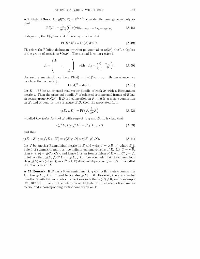
Appendix A Chern–Weil Theory 135
A.2 Euler Class. On gl(2r,R) = R2r×2r, consider the homogeneous polyno-mial
Pf(A) :=1
2rr!
∑
σ
ε(σ)aσ(1)σ(2) . . . aσ(2r−1)σ(2r) (A.48)
of degree r, the Pfaffian of A. It is easy to show that
Pf(BABt) = Pf(A) detB. (A.49)
Therefore the Pfaffian defines an invariant polynomial on so(2r), the Lie algebraof the group of rotations SO(2r). The normal form on so(2r) is
A =
A1
. . .
Ar
with Aj =
(0 −ajaj 0
). (A.50)
For such a matrix A, we have Pf(A) = (−1)ra1 . . . ar. By invariance, weconclude that on so(2r),
Pf(A)2 = detA. (A.51)
Let E → M be an oriented real vector bundle of rank 2r with a Riemannianmetric g. Then the principal bundle P of oriented orthonormal frames of E hasstructure group SO(2r). If D is a connection on P , that is, a metric connectionon E, and R denotes the curvature of D, then the associated form
χ(E, g,D) := Pf„
P,1
2πR
«
(A.52)
is called the Euler form of E with respect to g and D. It is clear that
χ(f∗E, f∗g, f∗D) = f∗χ(E, g,D) (A.53)
and that
χ(E ⊕ E′, g ⊕ g′, D ⊕D′) = χ(E, g,D) ∧ χ(E′, g′, D′). (A.54)
Let g′ be another Riemannian metric on E and write g′ = g(B · , ·) where B isa field of symmetric and positive definite endomorphisms of E. Let C =
√B,
then g′(x, y) = g(Cx,Cy), and hence C is an isomorphism of E with C∗g = g′.It follows that χ(E, g′, C∗D) = χ(E, g,D). We conclude that the cohomologyclass χ(E) of χ(E, g,D) in H2r(M,R) does not depend on g and D. It is calledthe Euler class of E.
A.55 Remark. If E has a Riemannian metric g with a flat metric connectionD, then χ(E, g,D) = 0 and hence also χ(E) = 0. However, there are vectorbundles E with flat non-metric connections such that χ(E) 6= 0, see for example[MS, 312 pp]. In fact, in the definition of the Euler form we need a Riemannianmetric and a corresponding metric connection on E.

136 Lectures on Kahler Manifolds
Our next aim is to compare Euler class and Chern classes. We identify Cr
with R2r via the correspondence
(z1, . . . , zr)←→ (x1, y1, . . . , xr, yr),
where zj = xj + iyj. This induces an inclusion U(r) → SO(2r) of the unitarygroup and a corresponding inclusion u(r) → so(2r), A 7→ AR, of Lie algebras.Under this inclusion, diagonal matrices
A =
ia1
. . .
iar
7→
A1
. . .
Ar
= AR, (A.56)
where Aj is as above. For such a diagonal A, det(iA) = (−1)ra1 . . . ar =Pf(AR). By invariance,
det(iA) = Pf(AR) (A.57)
for all A ∈ u(r).Suppose now that E →M is a complex vector bundle of rank r. Endow E
with a Hermitian metric h and a corresponding Hermitian connection D. If weconsider E as an oriented real vector bundle of rank 2r, the real part g = Rehof the Hermitian metric defines a Riemannian metric on E and D is metricwith respect to g.
Let ω and Ω be the connection and curvature forms of D with respect toa local unitary frame of E. If we consider E as an oriented real vector bundleand choose D as a metric connection for the Riemannian metric g as above,then ωR and ΩR are the connection and curvature forms of D with respect tothe induced oriented and orthonormal frame of E. By (A.33) and (A.57),
cr(E,D) = det„
i
2πΩ
«
= Pf„
1
2πΩR
«
= χ(E, g,D). (A.58)
A.59 Proposition. For a complex vector bundle E →M of rank r, χ(E) =cr(E).
Proposition A.59 and Equations A.53, A.54 imply that the Euler class of(the tangent bundle of) an oriented closed manifold M , applied to the fun-damental class of M , gives the Euler number of M . This is the celebratedChern–Gauß–Bonnet formula.
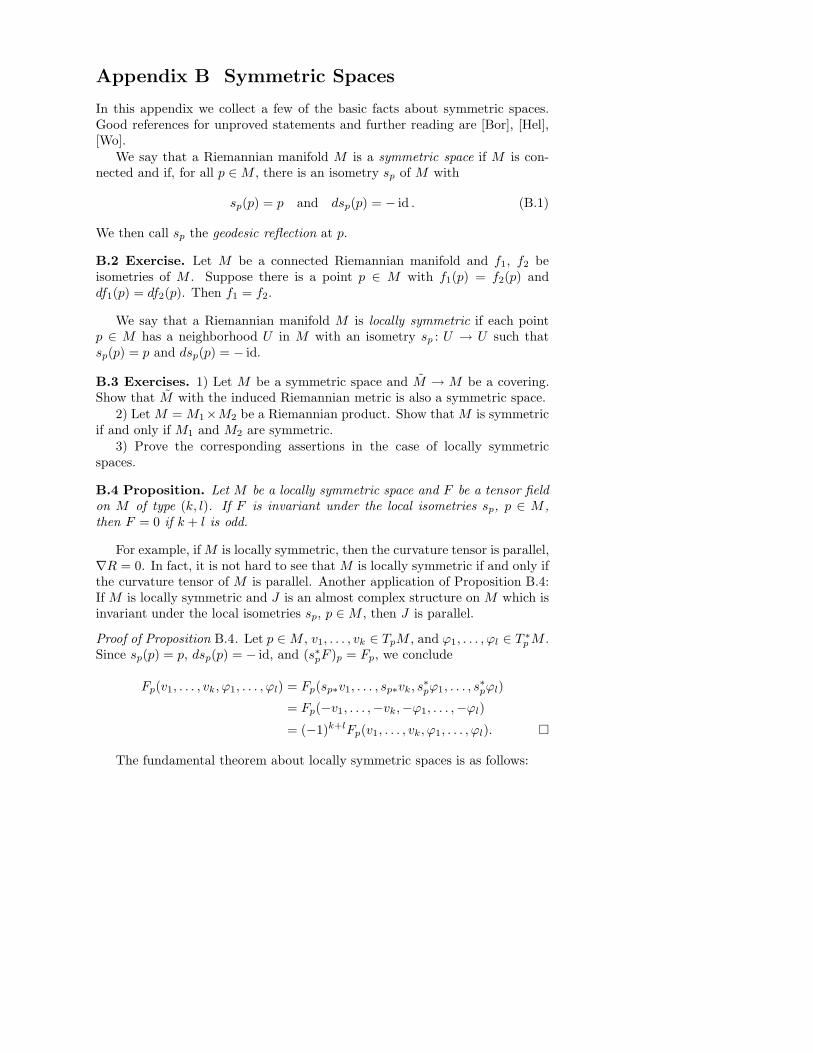
Appendix B Symmetric Spaces
In this appendix we collect a few of the basic facts about symmetric spaces.Good references for unproved statements and further reading are [Bor], [Hel],[Wo].
We say that a Riemannian manifold M is a symmetric space if M is con-nected and if, for all p ∈M , there is an isometry sp of M with
sp(p) = p and dsp(p) = − id . (B.1)
We then call sp the geodesic reflection at p.
B.2 Exercise. Let M be a connected Riemannian manifold and f1, f2 beisometries of M . Suppose there is a point p ∈ M with f1(p) = f2(p) anddf1(p) = df2(p). Then f1 = f2.
We say that a Riemannian manifold M is locally symmetric if each pointp ∈ M has a neighborhood U in M with an isometry sp : U → U such thatsp(p) = p and dsp(p) = − id.
B.3 Exercises. 1) Let M be a symmetric space and M → M be a covering.Show that M with the induced Riemannian metric is also a symmetric space.
2) Let M = M1×M2 be a Riemannian product. Show that M is symmetricif and only if M1 and M2 are symmetric.
3) Prove the corresponding assertions in the case of locally symmetricspaces.
B.4 Proposition. Let M be a locally symmetric space and F be a tensor fieldon M of type (k, l). If F is invariant under the local isometries sp, p ∈ M ,then F = 0 if k + l is odd.
For example, if M is locally symmetric, then the curvature tensor is parallel,∇R = 0. In fact, it is not hard to see that M is locally symmetric if and only ifthe curvature tensor of M is parallel. Another application of Proposition B.4:If M is locally symmetric and J is an almost complex structure on M which isinvariant under the local isometries sp, p ∈M , then J is parallel.
Proof of Proposition B.4. Let p ∈M , v1, . . . , vk ∈ TpM , and ϕ1, . . . , ϕl ∈ T ∗pM .
Since sp(p) = p, dsp(p) = − id, and (s∗pF )p = Fp, we conclude
Fp(v1, . . . , vk, ϕ1, . . . , ϕl) = Fp(sp∗v1, . . . , sp∗vk, s∗pϕ1, . . . , s
∗pϕl)
= Fp(−v1, . . . ,−vk,−ϕ1, . . . ,−ϕl)= (−1)k+lFp(v1, . . . , vk, ϕ1, . . . , ϕl).
The fundamental theorem about locally symmetric spaces is as follows:

138 Lectures on Kahler Manifolds
B.5 Theorem (Cartan). Let M and N be locally symmetric Riemannianspaces, where M is simply connected and N is complete. Let p ∈M and q ∈ N ,and let A : TpM → TqN be a linear isomorphism preserving inner products andcurvature tensors,A∗gNq = gMp and A∗RNq = RMp . Then there is a unique localisometry F : M → N with F (p) = q and F ′(p) = A.
As for a proof, see for example the more general Theorems 1.1.36 in [CEb]or III.5.1 in [Sa]23.
B.6 Corollary. Let M be a complete and simply connected locally symmetricspace. Then M is a symmetric space. More precisely, the differentials of theisometries of M fixing a point p in M are given precisely by the orthogonaltransformations of TpM preserving the curvature tensor RMp .
This is one of the most important immediate applications of Theorem B.5.Another immediate application asserts that a simply connected symmetricspace is determined, up to isometry, by the inner product and the curvaturetensor at a point (using Propositions B.7 and B.8 below). This implies, for ex-ample, the uniqueness of the model Riemannian manifolds of constant sectionalcurvature.
B.7 Proposition. If M is symmetric, then M is homogeneous.
Proof. Let c : [a, b] → M be a geodesic in M , and let m be the midpointof c. Then the geodesic reflection sm of M at m reflects c about m, hencesm(c(a)) = c(b).
Since M is connected, any two points p, q ∈ M can be connected by apiecewise geodesic c. If c : [a, b]→M is such a curve, then there is a subdivisiona = t0 < t1 < · · · < tk = b of [a, b] such that c|[ti−1, ti] is a geodesic, 1 ≤ i ≤ k.By the first part of the proof, there is an isometry fi of M mapping c(ti−1) toc(ti). Hence fk · · · f1 is an isometry of M mapping p = c(a) to q = c(b).
B.8 Proposition. If M is homogeneous, then M is complete.
Proof. Let p ∈ M . Then there is an ε > 0 such that the closed ball B(p, ε) of
radius ε about p is compact. Since M is homogeneous, the closed ball B(q, ε)of radius ε about any point q ∈ M is compact. It follows that M is complete.
Let M be a symmetric space. Let c : [a, b] → M be a piecewise smoothcurve. An isometry f : M → M is called transvection along c if f(c(a)) = c(b)and if df(c(a)) is equal to parallel translation along c from c(a) to c(b).
Let p be a point in M . Let c : R → M be a geodesic through p. Let st bethe geodesic reflection about c(t) and ft = st/2 s0. Then ft is an isometry ofM with ft(c(τ)) = c(τ + t) for all τ ∈ R.
23Both references contain also introductions to symmetric spaces.
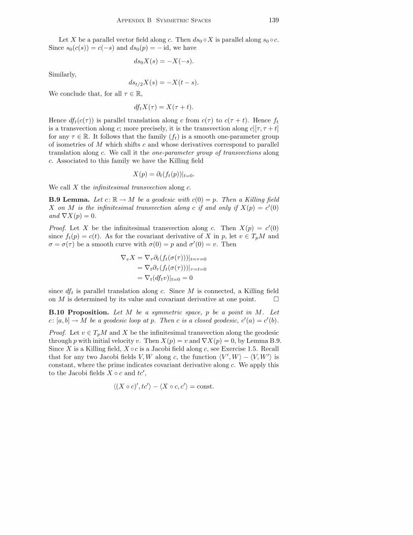
Appendix B Symmetric Spaces 139
Let X be a parallel vector field along c. Then ds0 X is parallel along s0 c.Since s0(c(s)) = c(−s) and ds0(p) = − id, we have
ds0X(s) = −X(−s).
Similarly,dst/2X(s) = −X(t− s).
We conclude that, for all τ ∈ R,
dftX(τ) = X(τ + t).
Hence dft(c(τ)) is parallel translation along c from c(τ) to c(τ + t). Hence ftis a transvection along c; more precisely, it is the transvection along c|[τ, τ + t]for any τ ∈ R. It follows that the family (ft) is a smooth one-parameter groupof isometries of M which shifts c and whose derivatives correspond to paralleltranslation along c. We call it the one-parameter group of transvections alongc. Associated to this family we have the Killing field
X(p) = ∂t(ft(p))|t=0.
We call X the infinitesimal transvection along c.
B.9 Lemma. Let c : R→M be a geodesic with c(0) = p. Then a Killing fieldX on M is the infinitesimal transvection along c if and only if X(p) = c′(0)and ∇X(p) = 0.
Proof. Let X be the infinitesimal transvection along c. Then X(p) = c′(0)since ft(p) = c(t). As for the covariant derivative of X in p, let v ∈ TpM andσ = σ(τ) be a smooth curve with σ(0) = p and σ′(0) = v. Then
∇vX = ∇τ∂t(ft(σ(τ)))|t=τ=0
= ∇t∂τ (ft(σ(τ)))|τ=t=0
= ∇t(dftv)|t=0 = 0
since dft is parallel translation along c. Since M is connected, a Killing fieldon M is determined by its value and covariant derivative at one point.
B.10 Proposition. Let M be a symmetric space, p be a point in M . Letc : [a, b]→M be a geodesic loop at p. Then c is a closed geodesic, c′(a) = c′(b).
Proof. Let v ∈ TpM and X be the infinitesimal transvection along the geodesicthrough p with initial velocity v. ThenX(p) = v and∇X(p) = 0, by Lemma B.9.Since X is a Killing field, X c is a Jacobi field along c, see Exercise 1.5. Recallthat for any two Jacobi fields V,W along c, the function 〈V ′,W 〉 − 〈V,W ′〉 isconstant, where the prime indicates covariant derivative along c. We apply thisto the Jacobi fields X c and tc′,
〈(X c)′, tc′〉 − 〈X c, c′〉 = const.
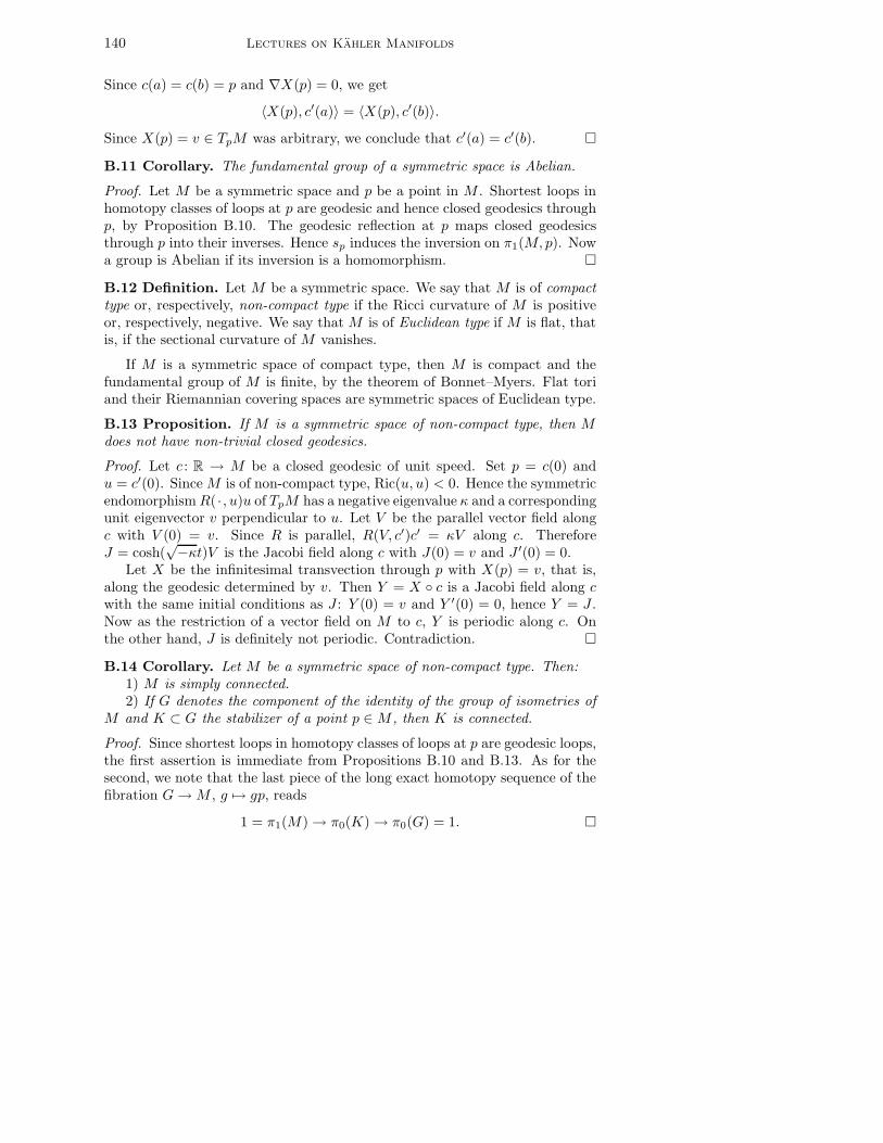
140 Lectures on Kahler Manifolds
Since c(a) = c(b) = p and ∇X(p) = 0, we get
〈X(p), c′(a)〉 = 〈X(p), c′(b)〉.Since X(p) = v ∈ TpM was arbitrary, we conclude that c′(a) = c′(b).
B.11 Corollary. The fundamental group of a symmetric space is Abelian.
Proof. Let M be a symmetric space and p be a point in M . Shortest loops inhomotopy classes of loops at p are geodesic and hence closed geodesics throughp, by Proposition B.10. The geodesic reflection at p maps closed geodesicsthrough p into their inverses. Hence sp induces the inversion on π1(M,p). Nowa group is Abelian if its inversion is a homomorphism.
B.12 Definition. Let M be a symmetric space. We say that M is of compacttype or, respectively, non-compact type if the Ricci curvature of M is positiveor, respectively, negative. We say that M is of Euclidean type if M is flat, thatis, if the sectional curvature of M vanishes.
If M is a symmetric space of compact type, then M is compact and thefundamental group of M is finite, by the theorem of Bonnet–Myers. Flat toriand their Riemannian covering spaces are symmetric spaces of Euclidean type.
B.13 Proposition. If M is a symmetric space of non-compact type, then Mdoes not have non-trivial closed geodesics.
Proof. Let c : R → M be a closed geodesic of unit speed. Set p = c(0) andu = c′(0). Since M is of non-compact type, Ric(u, u) < 0. Hence the symmetricendomorphismR( · , u)u of TpM has a negative eigenvalue κ and a correspondingunit eigenvector v perpendicular to u. Let V be the parallel vector field alongc with V (0) = v. Since R is parallel, R(V, c′)c′ = κV along c. ThereforeJ = cosh(
√−κt)V is the Jacobi field along c with J(0) = v and J ′(0) = 0.Let X be the infinitesimal transvection through p with X(p) = v, that is,
along the geodesic determined by v. Then Y = X c is a Jacobi field along cwith the same initial conditions as J : Y (0) = v and Y ′(0) = 0, hence Y = J .Now as the restriction of a vector field on M to c, Y is periodic along c. Onthe other hand, J is definitely not periodic. Contradiction.
B.14 Corollary. Let M be a symmetric space of non-compact type. Then:1) M is simply connected.2) If G denotes the component of the identity of the group of isometries of
M and K ⊂ G the stabilizer of a point p ∈M , then K is connected.
Proof. Since shortest loops in homotopy classes of loops at p are geodesic loops,the first assertion is immediate from Propositions B.10 and B.13. As for thesecond, we note that the last piece of the long exact homotopy sequence of thefibration G→M , g 7→ gp, reads
1 = π1(M)→ π0(K)→ π0(G) = 1.
Appendix B Symmetric Spaces 141
B.15 Remark. In Remark B.29 we show that a symmetric space has non-negative sectional curvature iff its Ricci curvature is non-negative and, simi-larly, that it has non-positive sectional curvature iff its Ricci curvature is non-positive. In particular, a symmetric space is of Euclidean type if and only ifits Ricci curvature vanishes. Furthermore, if M is a symmetric space of non-compact type, then M is diffeomorphic to Rn, n = dimM , by the theoremof Hadamard–Cartan and Corollary B.14.1. It follows that, for K and G asin Corollary B.14.2, K is a deformation retract of G. This improves Corol-lary B.14.2.
B.1 Symmetric Pairs. Let (G,K) be a pair consisting of a Lie group G anda closed subgroup K. We say that (G,K) is a symmetric pair if M = G/K isconnected and if there is an involutive automorphism σ : G→ G with
F0 ⊂ K ⊂ F, (B.16)
where F = g ∈ G | σ(g) = g and F0 denotes the component of the identity ofF . In what follows, (G,K) is a symmetric pair with involutive automorphismσ.
Let g be the Lie algebra of left-invariant vector fields of G, via evaluationidentified with the tangent space TeG of G at the neutral element e ∈ G.Denote by σ∗ the differential of σ at e, and let
k = X ∈ g | σ∗X = X, p = X ∈ g | σ∗X = −X, (B.17)
the eigenspaces of σ∗ for the eigenvalues 1 and −1, respectively. Since σ∗ isinvolutive,
g = k + p. (B.18)
Since F0 ⊂ K ⊂ F , k is the Lie algebra of K. Since K ⊂ F , σ(kgk−1) =kσ(g)k−1 for all k ∈ K and all g ∈ G, and hence σ∗ commutes with all Adk,k ∈ K. Therefore
Adk(k) ⊂ k and Adk(p) ⊂ p for all k ∈ K. (B.19)
Furthermore,[k, k] ⊂ k, [k, p] ⊂ p, [p, p] ⊂ k. (B.20)
In particular, k is perpendicular to p with respect to the Killing form of g. Asfor the proof of (B.20), the first and second inclusion follow from (B.19) above.For the proof of the third, let X,Y ∈ p. Since σ∗ is an automorphism of g, wehave
σ∗[X,Y ] = [σ∗X,σ∗Y ] = [−X,−Y ] = [X,Y ]
and hence [X,Y ] ∈ k. Note that the first two inclusions also follow by a similarargument.
142 Lectures on Kahler Manifolds
Since we divide by K on the right, G acts from the left on M . We denoteby gp ∈M the image of p ∈M under left multiplication by g ∈ G. Sometimesit will be convenient to distinguish between the element g ∈ G and the diffeo-morphism of M given by left multiplication with g. Then we will use λg todenote the latter, λg(p) := gp.
B.21 Exercise. Let M be a manifold and G be a Lie group which acts on M .For X ∈ g, define a smooth vector field X∗ on M by
X∗(p) = ∂t(etX(p))|t=0.
By definition, exp(tX) is the flow of X∗. Show that [X,Y ]∗ = −[X∗, Y ∗].
We denote by o = [K] the distinguished point of M and by π : G→M thecanonical map, π(g) = [gK] = λg(o). We use π∗ = dπ(e) : p→ ToM to identifyp and ToM . An easy computation shows that for all k ∈ K
π∗ Adk = dλk(o) π∗. (B.22)
Thus with respect to the identification p ∼= ToM via π∗, the isotropy represen-tation of K on ToM corresponds to the restriction of the adjoint representationof K to p.
We say that a symmetric pair is Riemannian if there is an inner product〈·, ·〉 on p which is invariant under AdK , that is, under all Adk, k ∈ K. Notethat such inner products are in one-to-one correspondence with G-invariantRiemannian metrics on M .
B.23 Example. Let M be a symmetric space and o ∈ M be a preferredorigin. Let G be the group Iso(M) of all isometries of M or the componentof the identity in Iso(M). Let K be the stabilizer of o in G. Then (G,K) isa Riemannian symmetric pair with respect to the involution σ of G given byconjugation with the geodesic reflection so of M in o. The pull back of theinner product in ToM to p is invariant under AdK and turns (G,K) into aRiemannian symmetric pair with G/K = M .
B.24 Theorem. Let (G,K) be a Riemannian symmetric pair with correspond-ing involution σ of G and inner product 〈· , ·〉 on p. Let M = G/K and endowM with the G-invariant Riemannian metric corresponding to 〈· , ·〉. Then wehave:
1. M is a symmetric space. The geodesic symmetry s at o is s([gK]) =[σ(g) ·K]. In particular, s λg = λσ(g) s.
2. For X ∈ p, the curve etX(o), t ∈ R, is the geodesic through o with initialvelocity π∗X, and left multiplication by etX , t ∈ R, is the one-parametergroup of transvections along this geodesic.
Appendix B Symmetric Spaces 143
3. With respect to the identification p ∼= ToM , AdK-invariant tensors on p
correspond to G-invariant tensor fields on M and these are parallel.
4. With respect to the identification p ∼= ToM , the curvature tensor R andRicci tensor Ric of M at o are given by
R(X,Y )Z = −[[X,Y ], Z] = −[[X∗, Y ∗], Z∗](p),
Ric(X,Y ) = −1
2B(X,Y ),
where B denotes the Killing form of g and X∗, Y ∗, Z∗ are associated toX,Y, Z as in Exercise B.21.
5. With respect to the identification p ∼= ToM , a subspace q ⊂ p is tangent toa totally geodesic submanifold of M through o if and only if [[q, q], q] ⊂ q.If the latter inclusion holds, then N = exp(q)(o) is such a submanifoldand is a symmetric space in the induced Riemannian metric.
B.25 Remarks. 1) We can rewrite the first formula in B.24.4 as follows:
R(X,Y ) = − ad[X,Y ] or R( · , Y )Z = − adZ adY ,
where X,Y, Z ∈ p and both maps are considered on p.2) The totally geodesic submanifold in B.24.5 need not be closed. A good
example for this is a non-rational line through 0 in a flat torus.
Proof of Theorem B.24. It is easy to see that s([gK]) := [σ(g) ·K] defines aninvolutive smooth map s of M with s λg = λσ(g) s. Since s is involutive, sis a diffeomorphism of M . Moreover s(o) = o and ds(o) = − id.
Let p = g(o) ∈ M and u ∈ TpM . Choose v ∈ ToM with dλg(v) = u. Bythe G-invariance of the metric, we have ‖u‖ = ‖dλg(v)‖ = ‖v‖ and hence
‖ds(u)‖ = ‖ds(dλg(v))‖ = ‖dλσ(g)(ds(v))‖ = ‖ − dλσ(g)(v)‖ = ‖v‖ = ‖u‖.
It follows that s is an isometry. This completes the proof of (1).Let X ∈ p and X∗ be the corresponding Killing field of M as in Exer-
cise B.21. Since X ∈ p, we have
etX(s(p)) = s(e−tX(p))
for all p ∈ M , hence s∗X∗ = −X∗. Let u ∈ ToM . Since s is an isometry, we
get−∇uX∗ = ds(∇uX∗) = ∇ds(u)(s∗X
∗) = ∇uX∗,
and hence ∇X∗(o) = 0. Hence X∗ is the infinitesimal transvection withX∗(o) = π∗X . This proves (2).
It is clear that AdK-invariant tensors on p correspond to G-invariant ten-sor fields on M . Now the one-parameter groups (exp(tX)), X ∈ p, are the
144 Lectures on Kahler Manifolds
transvections along the corresponding geodesics through o. It follows that G-invariant tensor fields are parallel at o and hence parallel everywhere in M .Hence (3).
Let X,Y, Z ∈ p and X∗, Y ∗, Z∗ be the corresponding Killing fields of M asin Exercise B.21. Then X∗ Y ∗, and Z∗ are parallel at o. Let u = Z∗(o) = π∗Zand compute ∇u[X∗, Y ∗] using the differential equation for Killing fields. Thisgives the first equation in (4). In the proof of the second we can assume thatX = Y , by the symmetry of the Ricci tensor. Since X ∈ p, we have adX(k) ⊂ p
and adX(p) ⊂ k. Therefore tr ad2X |k = tr ad2X |p, and the claim about theRicci tensor follows.
It remains to prove (5). Note that for a totally geodesic submanifold Nthrough the origin o, R(u, v)w ∈ ToN for all u, v, w ∈ ToN . Hence the necessityof the condition on q is immediate from the formula for R in (3).
Suppose now that [[q, q], q] ⊂ q. Let l = [q, q]. Then l is a Lie subalgebra of k
and h = l+q is a Lie subalgebra of g. Let H be the corresponding connected Liesubgroup of G. Then the orbit N of o under H , N = H(o), is a submanifold ofM . Now N is totally geodesic at o since N = exp(q)(o) locally about o. SinceH is transitive on N and H acts isometrically on M , N is totally geodesiceverywhere. Since M is a complete Riemannian manifold and N is connectedwe have N = exp(q)(o). In particular, N is complete. Since N is invariantunder s, s|N is the geodesic symmetry of N in o. Since N is homogeneous, Nis symmetric.
B.26 Remark (Coverings). The groups K with F0 ⊂ K ⊂ F correspond toRiemannian coverings
G/F0 → G/K → G/F.
For example, if M = Sn ⊂ Rn+1, the unit sphere of dimension n, then thecomponent G of the identity in Iso(M) is equal to SO(n+1). If we let s be thereflection in a chosen unit vector v ∈ Sn and σ be conjugation with s, then thestabilizer K of v is isomorphic to SO(n) and K = F0 6= F . If we pass to thequotient RPn keeping G, then we have K = F . A similar phenomenon occursfor some of the other symmetric spaces of compact type.
It is remarkable that the fixed point set of an involution of a compactand simply connected Lie group is connected, see [Hel, Theorem VII.7.2].Thus the symmetric space associated to a Riemannian symmetric pair (G,K)with G compact and simply connected is simply connected. For example,the unit sphere Sn is associated to the Riemannian symmetric pair (Spin(n +1), Spin(n)). Real projective space RPn is a homogeneous space of Spin(n+1),but is not associated to a Riemannian symmetric pair (G,K) with G simplyconnected.
B.27 Remark (Effective Pairs). Let (G,K) be a Riemannain symmetric pairand N ⊂ G be the normal subgroup of elements acting trivially on M = G/K,
N = g ∈ G | g acts as identity on M.
Appendix B Symmetric Spaces 145
Then N ⊂ K, hence the involution σ of G factors over G/N . Since M isconnected, an isometry of M = G/K fixing the preferred origin o of M isdetermined by its differential at o, see Exercise B.2. Hence
N = k ∈ K | Adk is the identity on p.
In particular, the adjoint action of K on p factors over K/N . It follows that(G/N,K/N) is a Riemannian symmetric pair with (G/N)/(K/N) = G/K = Mand Lie algebra g/n ∼= k/n + p.
We say that the Riemannian symmetric pair (G,K) is effective or, respec-tively, infinitesimally effective ifN is trivial or, respectively, a discrete subgroupof G. The pair (G,K) is effective iff G is a subgroup of the isometry groupof M . The above pair (G/N,K/N) is the effective pair associated to (G,K).Thus it becomes plausible that, for many purposes, it is sufficient to considereffective or infinitesimally effective pairs.
B.28 Remark (Killing Form). Let (G,K) be an infinitesimally effective Rie-mannian symmetric pair with K/N compact, where N is as in Remark B.27.Let X ∈ k. From (B.20) we know that adX(k) ⊂ k and adX(p) ⊂ p. Hence
B(X,X) = tr(adX |k)2 + tr(adX |p)2 = BK(X,X) + tr(adX |p)2,
where B is the Killing form of G and BK the Killing form of K. Since N ⊂ Kis a discrete subgroup and K/N is compact, BK ≤ 0 and hence B(X,X) ≤tr(adX |p)2. On the other hand, since N is discrete and X ∈ k, adX |p 6= 0 forX 6= 0, compare Exercise B.2. Furthermore, adX is skew-symmetric on p withrespect to the given inner product on p since the adjoint representation of K onp preserves this product. Now the square of a skew-symmetric endomorphismhas negative trace unless the endomorphism vanishes. Therefore B is negativedefinite on k. Hence G is semi-simple if and only if the Ricci curvature ofM = G/K is non-degenerate.
B.29 Remark (Curvature). Let (G,K) be an infinitesimally effective Rieman-nian symmetric pair with K/N compact, where N is as in Remark B.27. Sincethe Ricci tensor of M = G/K is parallel, there are real numbers λi and pairwiseperpendicular parallel distributions Ei on M such that RicX = λiX for all Xtangent to Ei. Identify p = ToM and let X,Y ∈ p be tangent to Ei and Ej ,respectively. Then, by Theorem B.24.4,
B([X,Y ], [X,Y ]) = −B([X, [X,Y ]], Y ) = 2 Ric([X, [X,Y ]], Y )
= 2λj〈[X, [X,Y ]], Y 〉 = −2λj〈R(Y,X)X,Y 〉,
where we use that Y is tangent to Ej . By the same computation,
B([Y,X ], [Y,X ]) = −2λi〈R(X,Y )Y,X〉.
146 Lectures on Kahler Manifolds
Hence B([X,Y ], [X,Y ]) = 0 if λi 6= λj or if λi = 0 or λj = 0. Since B isnegative definite on k, this implies that the curvature tensor R vanishes on thekernel of Ric. For λi 6= 0 and X,Y ∈ p both tangent to Ei, we get
〈R(X,Y )Y,X〉 = − 1
2λiB([X,Y ], [X,Y ]).
In particular, the sectional curvature of a symmetric space is non-negativerespectively non-positive iff its Ricci curvature is non-negative respectively non-positive.
By definition, M is of compact or, respectively, non-compact type iff allλi > 0 or, respectively, all λi < 0. In particular, a symmetric space of non-compact type is a complete and simply connected Riemannian manifold ofnon-positive sectional curvature, compare Corollary B.14 and Remark B.15.
If M is simply connected, the distributions Ei give rise to a splitting of Mas a Riemannian product with factors Mi tangent to Ei. For each i, Mi isa symmetric Einstein space with Einstein constant λi. Applying this to theuniversal covering space of M , we see that we can renormalize the metric of Mwithout destroying the geometry of M so that the constants λi are in ±1, 0.For example, if M is of compact type, we can renormalize the metric so thatM becomes an Einstein space with Einstein constant 1.
B.30 Remark (Curvature Operator). Let (G,K) be a Riemannian symmetricpair. Suppose that the inner product on p is the restriction of an AdG-invariantbilinear form24, also denoted 〈· , ·〉, on g. Then all adX , X ∈ g, are skew-symmetric with respect to 〈· , ·〉, and then, with respect to the identificationp = ToM ,
〈R(X,Y )V, U〉 = −〈[[X,Y ], V ], U〉 = 〈[X,Y ], [U, V ]〉. (B.31)
Recall the definition of the curvature operator R in (1.43) and define a mor-phism
F : Λ2p→ k, F (X ∧ Y ) := [X,Y ]. (B.32)
By (B.31), we have
〈R(X ∧ Y ), U ∧ V 〉 = 〈F (X ∧ Y ), F (U ∧ V )〉. (B.33)
In particular, if 〈· , ·〉 is an inner product on g, then
〈R(X,Y )Y,X〉 = |[X,Y ]|2 and R = F ∗F ≥ 0. (B.34)
Compare Remarks 1.42 and 5.56 for important consequences of R ≥ 0.
24For example, a negative or positive multiple of the Killing form of G if (G, K) is infini-tesimally effective and M = G/K is of compact or non-compact type, respectively.
Appendix B Symmetric Spaces 147
B.35 Remark (De Rham Decomposition). Let M be a simply connected sym-metric space. If N is a factor in the de Rham decomposition of M , then N istangent to one of the distributions Ei as in Remark B.29 (but TN might besmaller than Ei). From Remark B.29 we conclude that N is an Einstein space.Let λ be the Einstein constant of N . We have:
1) If λ < 0, then N is a symmetric space of non-compact type.
2) If λ = 0, then N is a Euclidean space.
3) If λ > 0, then M is of compact type.
In particular, a compact symmetric space is of compact type if and only ifits fundamental group is finite.
B.36 Remark (Holonomy). Let (G,K) be a Riemannian symmetric pair andset M = G/K. Then π : G→M is a principal bundle with structure group K.The tangent bundle TM is (canonically isomorphic to) the bundle G×K p asso-ciated to the adjoint representation of K on p. The left-invariant distributionon G determined by p is a principal connection which induces the Levi-Civitaconnection on M . In particular, the holonomy group Hol(M) of M at o = [K]is contained in the image of K under the adjoint representation on p.
Assume now that (G,K) is infinitesimally effective with K/N compact,where N is as in Remark B.27. Suppose furthermore that the Ricci curvatureof M is non-degenerate. By (B.20), h = [p, p] + p is an ideal in g. By RemarkB.29, B|k is negative definite. By assumption, B|p is non-degenerate. Moreover,k and p are perpendicular with respect to B, by (B.20). In particular, G issemi-simple and B|h is non-degenerate with p ⊂ h. Hence the B-perpendicularcomplement h⊥ of h is contained in k and h ∩ h⊥ = 0. Since h is an ideal in g,h⊥ is an ideal as well. Hence [h, h⊥] = 0. We conclude that for X ∈ h⊥,
etXeY e−tX = eY
for all Y ∈ p and t ∈ R. Since exp(tX) ∈ K, this implies that exp(tX) acts asthe identity on M . Hence X = 0 since (G,K) is infinitesimally effective. Weconclude that g = h, that is k = [p, p].
For X,Y ∈ p, [X,Y ] ∈ k and the curvature tensor is R(X,Y ) = − ad[X,Y ]
on p. Moreover, the endomorphisms R(X,Y ) are in the Lie algebra of theholonomy group Hol(M). Hence, under the above assumptions on (G,K), theadjoint image of the component K0 of the identity of K is equal to the reducedholonomy group of M . In particular, if (G,K) is effective and M is of compactor non-compact type, then K0 is equal to the reduced holonomy group of M .If, moreover, M is simply connected and G is connected, then K is equal tothe holonomy group of M at the preferred origin and hence G is equal to thecomponent of the identity of the isometry group of M . Then parallel tensorson M are also G-invariant, compare Theorem B.24.3 for the converse assertion.
B.37 Exercise (Dual Pairs). Let (G,K) be a Riemannian symmetric pair and
148 Lectures on Kahler Manifolds
g = k+ p be the associated decomposition of the Lie algebra g of G. Show that
[X,Y ]′ :=
[X,Y ] if X ∈ k,
−[X,Y ] if X,Y ∈ p
defines a (new) Lie bracket on g. Note that this change corresponds to passingfrom g to g′ = k+ ip in the complexification gC of g. We say that a Riemanniansymmetric pair (G′,K ′) is dual to (G,K) if the corresponding decompositionof the Lie algebra g′ of G′ is up to isomorphism given by g′ = k + p with Liebracket [ · , · ]′. We also say that the corresponding symmetric spaces are dual.Show:
1) Under duality, the curvature tensor changes sign and compact type cor-responds to non-compact type.
2) For each symmetric space M , there is a simply connected symmetricspace M ′ dual to M and M ′ is unique up to isometry.
3) If M and N are simply connected dual symmetric spaces and K re-spectively L denotes the group of isometries fixing a point p ∈ M respec-tively q ∈ N , then there is an orthogonal transformation A : TpM → TqN withA∗RNq = −RMp and, for any such transformation, L = AKA−1.
B.2 Examples. This subsection is devoted to examples which are relevantin our discussion. To keep the presentation transparent, we divide them intothree classes, Examples B.38, B.42, and B.53.
B.38 Example. Let G = Sl(n,R) with involution σ(A) := (At)−1. The set offixed points of σ is K = SO(n). The map
G/K → Rn2
, AK 7→ AAt,
identifies G/K with the space of positive definite symmetric (n × n)-matriceswith determinant 1. We view these as the space of normalized inner productson Rn, or, more geometrically via their unit balls, as the space of ellipsoids inRn with volume equal to the volume of the Euclidean unit ball. We have
g = sl(n,R) = A ∈ Rn2 | trA = 0,
k = so(n) = U ∈ sl(n,R) | U t = −U,p = X ∈ sl(n,R) | Xt = X.
The symmetric bilinear form
〈A,B〉 = trAB (B.39)
on Rn2
is invariant under the adjoint action of Gl(n,R). Its restriction to p
is positive definite and turns (G,K) into a Riemannian symmetric pair. Since
Appendix B Symmetric Spaces 149
〈· , ·〉 is AdG-invariant, each adA, A ∈ g, is skew-symmetric with respect to〈· , ·〉. Therefore we have, for X,Y, Z ∈ p,
〈R(X,Y )Y,X〉 = 〈[X,Y ], [X,Y ]〉 ≤ 0, (B.40)
where we note that 〈· , ·〉 is negative definite on k.
The complexification is gC = sl(n,C) = A ∈ Cn2 | trA = 0. We see that
k + ip = su(n) = U ∈ sl(n,C) | U t = −U.
Hence (SU(n), SO(n)) is a dual pair to (Sl(n,R), SO(n)), where the involutionon SU(n) is given by the passage to the conjugate matrix. See also Exer-cise B.59.
B.41 Exercises. 1) Discuss (Gl(n,R),O(n)) as a symmetric pair.2) Show that Sl(2,R)/ SO(2) with the above Riemannian metric has con-
stant negative curvature −2 and construct isometries to some (other) modelsof the hyperbolic plane (with curvature −2).
B.42 Example. We show that the Grassmann manifold GF(p, q) of p-planesin Fp+q together with a natural Riemannian metric is a Riemannian symmetricspace, where F = R, C, or H. We also discuss the dual symmetric spaceG−
F(p, q). These symmetric spaces are also discussed in Examples 2.2.4, 4.10.5,
4.10.6, and B.83.1.Let G = O(p+q), U(p+q), and Sp(p+q) for F = R,C, and H, respectively25.
The natural action of G on GF(p, q) is transitive26. The stabilizer of the p-planeFp×0 ⊂ Fp+q isK = O(p)×O(q),U(p)×U(q), and Sp(p)×Sp(q), respectively,hence GF(p, q) = G/K.
Let S be the reflection of Fp+q about Fp × 0. Then conjugation with Sis an involutive automorphism of G with K as its set of fixed points. Hence(G,K) is a symmetric pair.
We write square (p + q)-matrices as blocks of four matrices correspondingto the preferred decomposition Fp+q = Fp × Fq. In this notation
k =
(U 00 V
) ∣∣ U t = −U, V t = −V, (B.43)
p =
(0 −Xt
X 0
) ∣∣ X ∈ Fq×p
∼= F
q×p. (B.44)
We write(A 00 B
)=: D(A,B) and
(0 −Xt
X 0
)=: P (X). (B.45)
25For the definition of Sp(n), see the discussion after (B.69).26We multiply vectors in Hp+q with scalars from the right and with matrices from the left.
150 Lectures on Kahler Manifolds
For D(A,B) ∈ K, D(U, V ) ∈ k, and P (X), P (Y ) ∈ p, we have
AdD(A,B) P (X) = P (BXAt),
[D(U, V ), P (X)] = P (V X −XU),
[P (X), P (Y )] = D(Y tX −XtY, Y Xt −XY t).
There is an AdG-invariant inner product on g,
〈A,B〉 =1
2Re tr(AtB). (B.46)
Its restriction to p turns (G,K) into a Riemannian symmetric pair. Withrespect to the identification P of Fq×p with p above, the curvature tensor ofGF(p, q) is given by
R(X,Y )Z = XY tZ + ZY tX − Y XtZ − ZXtY. (B.47)
By the AdG-invariance of the inner product on g,
〈R(X,Y )Y,X〉 = |[X,Y ]|2 ≥ 0. (B.48)
Hence the sectional curvature of GF(p, q) is non-negative.Inside GF(p, q), we consider the open subset G−
F(p, q) of p-planes on which
the non-degenerate form
Qp,q(x, y) = −∑
j≤p
xjyj +∑
j>p
xjyj (B.49)
on Fp+q is negative definite. Let G− = O(p, q), U(p, q), and Sp(p, q), respec-tively, be the group of linear transformations of Fp+q preserving this form.Then G− is transitive on G−
F(p, q) and G−
F(p, q) = G−/K, where K is as above.
Conjugation with the reflection S of Fp+q about Fp × 0 is an involutiveautomorphism of G− which has K as its set of fixed points. Hence (G−,K) isa symmetric pair as well. Now we have
p =
(0 Xt
X 0
) ∣∣ X ∈ Fq×p
∼= F
q×p, (B.50)
whereas K and k are as above. We write(
0 Xt
X 0
)= P−(X).
Then
[D(U, V ), P−(X)] = P−(V X −XU),
[P−(X), P−(Y )] = D(XtY − Y tX,XY t − Y Xt).
Appendix B Symmetric Spaces 151
We see that with respect to the identifications P and P− of p with Fq×p above,the Lie bracket [k, p] remains the same, but the Lie bracket [p, p] changes sign.That is, GF(p, q) and G−
F(p, q) are dual symmetric spaces in the sense of Ex-
ercise B.37. There is a corresponding change in sign for curvature tensor andsectional curvature.
B.51 Exercise. Show that the Riemannian metrics on GF(p, q) and G−F
(p, q)are Einsteinian with Einstein constant k(p+ q + 2)− 4 and −k(p+ q + 2) + 4,respectively, where k = dimR F.
B.52 Exercises. 1) Find other representations of Grassmannians as homoge-neous spaces, GF(p, q) = G/K, and discuss which of the corresponding pairs(G,K) are Riemannian symmetric pairs.
2) Replacing orthogonal groups by special orthogonal groups, we obtainthe Grassmann manifold Go
R(p, q) of oriented p-planes in Rp+q as homogeneous
space G/K, where G = SO(p+q) andK = SO(p)×SO(q). The same involutionσ as above, namely conjugation with the reflection S, leaves G invariant; withrespect to it k and p remain the same as before. Keeping the formula for theinner product on p, the formula for the curvature tensor remains the same.The natural “forget the orientation” map Go
R(p, q) → GR(p, q) is a twofold
Riemannian covering. If p+ q ≥ 3, then GoR(p, q) is simply connected.
3) A complex subspace of dimension p in Cn is also a real subspace ofR2n = Cn of dimension 2p, and similarly with Hn. Discuss the correspondinginclusions of Grassmann manifolds.
B.53 Example. Let V be a vector space over a field F . A symplectic form onV is an alternating two-form ω on V such that for all non-zero v ∈ V there isa vector w ∈ V with ω(v, w) 6= 0. A symplectic vector space is a vector spacetogether with a symplectic form. The standard example is F 2n with the form
ω((x, y), (u, v)) =∑
(xµvµ − yµuµ).
As in this example, the dimension of a finite-dimensional symplectic vectorspace V is even, dimV = 2n, and V has a basis (e1, . . . , en, f1, . . . , fn) suchthat
ω(eµ, eν) = ω(fµ, fν) = 0 and ω(eµ, fν) = δµν ,
a symplectic basis of V . The choice of a symplectic basis identifies V with thestandard symplectic vector space F 2n.
Let V be a symplectic vector space over a field F with symplectic formω. An endomorphism A : V → V is called symplectic if the pull back A∗ω =ω. Since ω is non-degenerate, symplectic endomorphisms are invertible, henceautomorphisms. Under composition, the set of all symplectic automorphismsof V is a group, denoted Sp(V ) and, respectively, Sp(n, F ) if V = F 2n. Let
J =
(0 1−1 0
)∈ Gl(2n, F ) (B.54)
152 Lectures on Kahler Manifolds
be the fundamental matrix of the standard symplectic form ω in F 2n, wherehere and below scalars represent the corresponding multiple of the unit matrixor block. Then a linear map g ∈ Gl(2n, F ) is in Sp(n, F ) if and only if gtJg = J .Writing g as a matrix of (n× n)-blocks,
g =
(A BC D
), (B.55)
the condition gtJg = J is equivalent to the conditions
AtC = CtA, BtD = DtB, and AtD − CtB = 1. (B.56)
It follows that the group of g ∈ Sp(n, F ) with B = C = 0 is an embeddedgeneral linear group,
Gl(n, F )→ Sp(n, F ), A 7→(A 00 (At)−1
). (B.57)
This induces the diagonal embedding of O(n, F ) into O(2n, F ).A subspace L of V is isotropic if ω(v, w) = 0 for all v, w ∈ L. A subspace
of V is called a Lagrangian subspace if it is a maximal isotropic subspace. Ifthe dimension of V is 2n, then Lagrangian subspaces of V have dimension n. If(e1, . . . , en, f1, . . . , fn) is a symplectic basis of V , then the subspace L0 spannedby e1, . . . , en is Lagrangian. We denote by G(L, V ) and GF (L, n) the space ofLagrangian subspaces of V and F 2n, respectively.
Let F = R and identify R2n = Cn by writing (x, y) = x+ iy = z. We have
〈v, w〉 = Re〈v, w〉 + iω(v, w),
where the left hand side is the standard Hermitian form on Cn and whereRe〈v, w〉 and ω(v, w) are the Euclidean inner product and the standard sym-plectic form on R2n, respectively. The real subspace L0 spanned by the unitvectors e1, . . . , en in Cn is Lagrangian. If L is any other Lagrangian subspaceof V and (b1, . . . , bn) is an orthonormal basis of L, then (b1, . . . , bn) is a unitarybasis of Cn with its standard Hermitian form 〈v, w〉. Therefore the naturalaction of U(n) on Cn induces a transitive action on GR(L, n) with stabilizerO(n) of L0, hence
GR(L, n) = U(n)/O(n). (B.58)
Let S : Cn → Cn be the real automorphism S(z) = z corresponding to the
reflection S(x, y) = (x,−y) of R2n. Then we have σ(A) := SAS−1 = A for anyA ∈ U(n). Hence the involution σ on U(n) has O(n) as its set of fixed points,turning (U(n),O(n)) into a Riemannian symmetric pair. Thus GR(L, n) is asymmetric space of dimension n(n + 1)/2 and a totally geodesic submanifoldof the Grassmannian GR(n, n).
Appendix B Symmetric Spaces 153
B.59 Exercise. We say that a Lagrangian subspace L of V = Cn (as above)is special if the n-form dz1 ∧ · · · ∧ dzn is real valued on L. Show that theabove Lagrangian subspace L0 is special, that the space GR(SL, n) of all spe-cial Lagrangian subspaces of V is given by the submanifold SU(n)/ SO(n) ofGR(L, n) = U(n)/O(n), and that GR(SL, n) is totally geodesic in GR(L, n).
Under the above identification R2n = Cn, A ∈ O(2n) is complex linear iffthe pull back A∗ω = ω. In other words,
U(n) = O(2n) ∩ Sp(n,R). (B.60)
Write g ∈ U(n) as g = A+ iB with real (n× n)-matrices A and B. Then thisidentification reads
U(n) ∋ A+ iB ←→(A −BB A
)∈ O(2n) ∩ Sp(n,R), (B.61)
where AtB = BtA and AtA+BtB = 1. In particular, O(n) = O(n,R) ⊂ U(n)is diagonally embedded in O(2n) ∩ Sp(n,R), compare with (B.57) above.
The symmetric space Gl(n,R)/O(n) is dual to U(n)/O(n) = GR(L, n) inthe sense of Exercise B.37. Motivated by the example of the Grassmannians,we would like to see if we can view Gl(n,R)/O(n) as the open set G−
R(L, n) ⊂
GR(L, n) of Lagrangian subspaces on which the symmetric form Qn,n from(B.49) is negative definite.
To that end, let O(n, n) be the orthogonal group of Qn,n. Clearly g ∈Gl(2n,R) belongs to O(n, n) iff
AtB = CtD, AtA− CtC = 1, and DtD −BtB = 1, (B.62)
where we write g as a matrix of blocks as in (B.55). Let g ∈ O(n, n)∩Sp(n,R).By (B.56) and (B.62),
B = (At)−1CtD = CA−1D. (B.63)
Writing D = AX , we compute
(1 + CtC)X = AtAX = AtD = 1 + CtB = 1 + CtCX. (B.64)
Hence X = 1, and hence D = A and B = C. We conclude that the intersectionO(n, n) ∩ Sp(n,R) consists of the matrices
(A BB A
)(B.65)
with AtB = BtA and AtA − BtB = 1. We also see that the subgroup ofmatrices in O(n, n) ∩ Sp(n,R) with B = 0 is a diagonally embedded O(n).
154 Lectures on Kahler Manifolds
Let L0 ∈ G−R
(L, n) be the Lagrangian subspace spanned by the first n unitvectors. Let L ∈ G−
R(L, n) be another Lagrangian subspace. Let (b1, . . . , bn)
be an orthogonal basis of L, that is, Qn,n(bj , bk) = −δjk. Let A and B bethe (n× n)-matrices with columns the first n and the last n coordinates of thevectors bj , respectively. Since L is Lagrangian and (b1, . . . , bn) is an orthogonalbasis of L, the corresponding matrix g as in (B.65) belongs to O(n, n)∩Sp(n,R).Since g maps L0 to L, we conclude that O(n, n) ∩ Sp(n,R) is transitive onG−
R(L, n). The stabilizer of L0 is the subgroup of matrices in O(n, n)∩Sp(n,R)
with B = 0, hence
G−R
(L, n) = (O(n, n) ∩ Sp(n,R))/O(n). (B.66)
Let
k :=1√2
(1 1−1 1
)∈ O(2n) ∩ Sp(n,R). (B.67)
We have
kGl(n,R)k−1 = O(n, n) ∩ Sp(n,R),
kO(n)k−1 = O(n),(B.68)
where we consider O(n) and Gl(n,R) as embedded subgroups in Sp(n,R) asabove. We conclude that conjugation with k identifies Gl(n,R)/O(n) with
(O(n, n) ∩ Sp(n,R))/O(n) = G−R
(L, n). (B.69)
Let F = C and identify C2n = Hn by writing z ∈ Hn as z = x + jy withx, y ∈ C2n, where we multiply with scalars from the right. We have z = x− jyand jx = xj. For z = x+ jy and w = u+ jv in Hn, we get
〈z, w〉 = 〈x− jy, u+ jv〉= (〈x, u〉+ 〈y, v〉) + j(〈x, v〉 − 〈y, u〉)= ((x, y), (u, v)) + jω((x, y), (u, v)),
where the first term on the right corresponds to the standard Hermitian formand ω to the standard symplectic form on C2n. The group of quaternionic(n×n)-matrices preserving the form 〈z, w〉 on Hn is called the symplectic group,denoted Sp(n). Considered as linear maps on C2n, elements of Sp(n) preservethe Hermitian form and the symplectic form on C2n. For any unit quaterniona,
〈az, aw〉 = 〈za, aw〉 = 〈z, w〉,so that left multiplication by a defines an element of Sp(n).
The complex subspace spanned by the unit vectors e1, . . . , en in Hn ∼= C2n
is Lagrangian. If L ⊂ C2n is any Lagrangian subspace of C2n and (b1, . . . , bn)
Appendix B Symmetric Spaces 155
is a unitary basis of L, then 〈bµ, bν〉 = δµν . Hence mapping the standard basis(e1, . . . , en) of Hn to (b1, . . . , bn) defines an element of Sp(n). It follows that
GC(L, n) = Sp(n)/U(n). (B.70)
The automorphism s(x + jy) = x − jy of H induces a complex automorphismS : Hn → Hn, defined by the analogous formula S(x + jy) = x − jy. Wesee that S corresponds to the reflection S(x, y) = (x,−y) of C2n. Since s isan automorphism of H, we have SAS−1 = σ(A), where σ(A) is the matrixobtained by applying s to the entries of A. Clearly σ is an involution of Sp(n)with U(n) as its set of fixed points, turning (Sp(n),U(n)) into a Riemanniansymmetric pair. Thus GC(L, n) is a symmetric space of dimension n(n + 1)and a totally geodesic submanifold of GC(n, n). Since the center of U(n) is notdiscrete, GC(L, n) is a Hermitian symmetric space, see Proposition B.86.
Under the identification C2n = Hn, A ∈ U(2n) is quaternion linear if andonly if the pull back A∗ω = ω. In other words,
Sp(n) = U(2n) ∩ Sp(n,C). (B.71)
Write g ∈ Sp(n) as g = A+ jB with complex (n×n)-matrices A and B. Thenthis identification reads
Sp(n) ∋ A+ jB ←→(A −BB A
)∈ U(2n) ∩ Sp(n,C), (B.72)
where AtB = BtA and AtA + BtB = 1. In particular, U(n) ⊂ Sp(n) is
diagonally embedded in U(2n) with blocks A and A on the diagonal.Again we want to identify the dual symmetric space Sp(n,R)/U(n) with
the open subset G−C
(L, n) ⊂ GC(L, n) of Lagrangian subspaces on which theHermitian form Qn,n from (B.49) is negative definite, where U(n) = O(2n) ∩Sp(n,R) as in (B.60).
We proceed as in the real case. First of all we note that g ∈ Gl(2n,C)belongs to the unitary group U(n, n) of Qn,n iff
AtB = CtD, AtA− CtC = 1, and DtD −BtB = 1, (B.73)
where we write g as a matrix of blocks as in (B.55). Let g ∈ U(n, n)∩Sp(n,C).By (B.56) and (B.73),
B = (At)−1CtD = CA−1D. (B.74)
Writing D = AX , we compute
(1 + CtC)X = AtAX = AtD = 1 + CtCX, (B.75)
156 Lectures on Kahler Manifolds
hence X = 1, and hence D = A and C = B. We conclude that the intersectionU(n, n) ∩ Sp(n,C) consists of the matrices
(A B
B A
)(B.76)
with AtB = BtA and AtA−BtB = 1. The subgroup of g ∈ U(n, n)∩ Sp(n,C)with B = 0 is a diagonally embedded U(n) as above. As in the real case, weget
G−C
(L, n) = (U(n, n) ∩ Sp(n,C))/U(n). (B.77)
Let
k :=1√2
(1 ii 1
)∈ U(2n) ∩ Sp(n,C). (B.78)
We have k−1 = k and hence
kk−1 = k2 =
(0 ii 0
). (B.79)
Let g ∈ Sp(n,C). Then k−1gk ∈ Sp(n,R) iff k−1gk = k−1gk, that is, iff
kk−1g = gkk−1. The latter holds iff D = A and C = B, that is, iff g ∈U(n, n) ∩ Sp(n,C). We conclude that
k Sp(n,R)k−1 = U(n, n) ∩ Sp(n,C). (B.80)
We also havek(O(2n) ∩ Sp(n,R))k−1 = U(n), (B.81)
where we consider U(n) on the right as an embedded subgroup in Sp(n,C) asabove. We finally conclude that conjugation with k identifies Sp(n,R)/U(n)with
(U(n, n) ∩ Sp(n,C))/U(n) = G−C
(L, n). (B.82)
Since the center of U(n) is not discrete, G−C
(L, n) is a Hermitian symmetricspace, see Remark B.87. Moreover, G−
C(L, n) is biholomorphic to the Siegel
upper half plane. For more on this, see e.g. [Bu, Section 31] or [Hel, ExerciseVIII.B].
B.3 Hermitian Symmetric Spaces. A Hermitian symmetric space is asymmetric space M together with a parallel almost complex structure on Mwhich is compatible with the Riemannian metric on M in the sense of (2.33).Since parallel almost complex structures are complex structures, any such struc-ture turns M into a Kahler manifold.
Symmetric spaces of non-compact type are simply connected (Corollary B.14),but there are symmetric spaces of compact type with non-trivial fundamental
Appendix B Symmetric Spaces 157
group. However, Hermitian symmetric spaces of compact type are Fano mani-folds and therefore simply connected, by Theorem 6.1227.
Let (G,K) be a Riemannian symmetric pair. Then by Theorem B.24.3,compatible parallel complex structures on M = G/K correspond to complexstructures on p which preserve the inner product on p and are invariant underthe adjoint action of K on p.
B.83 Examples. 1) Complex Grassmannians. We follow the notation in Ex-ample B.42 and consider
GC(p, q) = U(p+ q)/U(p)× U(q) = G/K,
the Grassmannian of complex p-planes in Cp+q, endowed with the Riemannianmetric introduced in (B.46). We define a complex structure on p by
JP (X) := P (iX),
where X ∈ Cq×p and P (X) ∈ p is defined as in (B.45). For D(A,B) ∈ K
we have AdD(A,B) P (X) = P (BXAt), hence J commutes with AdK , turningGC(p, q) into a Hermitian symmetric space.
The curvature tensor of GC(p, q) is given in (B.48). For p = 1, that is, inthe case of complex projective space, we get
R(X,Y )Y = 〈Y, Y 〉X − 〈X,Y 〉Y + 3〈X, JY 〉JY.
Thus the holomorphic sectional curvature of complex projective space is con-stant equal to 4 and the range of its sectional curvature is [1, 4]. We recommendKarcher’s article [Kar] for a nice exposition of the elementary geometry of com-plex projective spaces.
To compare the Riemannian metric onGC(p, q) here with the one introducedin Example 4.10, we note that both are invariant under the action of U(p+ q).Thus it suffices to compare them at the plane spanned by the first p unit vectors.For X ∈ p, we have
etX =
(1 −tXt
tX 1
)+ o(t).
Comparing with (4.14), we get that the Riemannian metric there is twice theRiemannian metric discussed here.
The discussion in the case of the dual Grassmannians G−C
(p, q) is similar.The case p = 1 is of particular importance, U(1,m)/U(1) × U(m) =: CHm iscalled complex hyperbolic space. It is dual to complex projective space. Withrespect to the given normalization of the Riemannian metric, the range of itssectional curvature is [−4,−1].
27There are more direct proofs for the latter assertion which do not rely on Kobayashi’stheorem, see e.g. [Hel, Theorem VIII.4.6].

158 Lectures on Kahler Manifolds
2) Complex quadric. Consider the Grassmannian manifold GoR(2, n− 2) of
oriented real 2-planes in Rn as in Exercise B.52.2,
GoR(2, n− 2) = SO(n)/ SO(2)× SO(n− 2).
There is a complex structure J on p which is invariant under the adjoint repre-sentation of SO(2)×SO(n−2): Identify R(n−2)×2 ∼= Cn−2, that is, think of thetwo columns of X ∈ R(n−2)×2 as real and imaginary part of a vector in Cn−2,and multiply this vector by i. Thus Go
R(2, n−2) together with the Riemannian
metric induced by the inner product on p and the parallel complex structureinduced by J is a Kahler manifold.
We can think of GoR(2, n− 2) as the complex quadric
Q = [z] ∈ CPn−1 | z21 + · · ·+ z2
n = 0. (B.84)
To that end, extend the action of SO(n) on Rn complex linearly to Cn torealize SO(n) as a subgroup of U(n). Let p0 = [1, i, 0, . . . , 0] ∈ Q. The orbit ofp0 under the induced action of SO(n) on CPn−1 is equal to Q. The stabilizerof p0 is SO(2)×SO(n−2), thus Q = SO(n)/ SO(2)×SO(n−2) = Go
R(2, n−2).
To compare the metric chosen above with the one on CPn−1, we let
A =
(A2
1n−2
)with A2 =
1√2
(1 ii 1
),
where 1r denotes the unit matrix of size r × r. Since A is unitary, A inducesan isometry of CPn−1. Moreover, A maps p1 = [1, 0, . . . , 0] to p0. For X ∈ p,we get
etXp0 = etXAp1 = A(A−1etXA)p1.
We have
A−1etXA =
(12 −tAt2Xt
tXA2 1n−2
)+ o(t).
Since the speed of the curve etXp0 at t = 0 is equal to the speed of the curve(A−1etXA)p1 at t = 0, we get that the Riemannian metric induced from CPn−1,normalized as in Example 1 above, is equal to the chosen metric on Go
R(2, n−2).
Intersecting two-planes with the unit sphere Sn−1, we identify GoR(2, n− 2)
with the space of oriented great circles on Sn−1. In particular, GoR(2, 1) is a
two-sphere or, what amounts to the same, a complex projective line. Thus thequadric Q ⊂ CP 2 in (B.84) is a complex projective line.
B.85 Remark. Let M be a simply connected Hermitian symmetric space withcomplex structure J , and let p be a point in M . Then Jp is the differential of anisometry jp of M fixing p, by Corollary B.6 and (4.43). By Exercise B.2, jp is inthe center of the group of holomorphic isometries ofM fixing p. Moreover, sinceJp is skew-symmetric and orthogonal, the endomorphisms cosx · id + sinx · Jpof TpM preserve metric and curvature tensor. Hence, by Corollary B.6, jpbelongs to the component of the identity of the stabilizer of p in the group ofholomorphic isometries of M .
Appendix B Symmetric Spaces 159
Recall the definition of infinitesimally effective from Remark B.27.
B.86 Proposition. Let (G,K) be an infinitesimally effective Riemannian sym-metric pair with G and K compact and connected. Assume that G is semi-simple and that the adjoint representation of K on p is irreducible. ThenM = G/K admits a G-invariant complex structure compatible with the Rie-mannian metric on M if and only if the center of K is not discrete, that is, ifand only if K is not semi-simple. If the latter holds, then M is a Hermitiansymmetric space of compact type, hence simply connected. If, moreover, (G,K)is effective, then the center ZK of K is a circle and J is (any) one of the twoelements of order 4 in ZK.
Proof. Since G is compact and semi-simple, M is a symmetric space of compacttype. Furthermore, π1(G) is finite and π2(G) = 0. The final part of the longexact homotopy sequence associated to the fiber bundle G→ G/K = M is
0 = π2(G)→ π2(M)→ π1(K)→ π1(G)→ π1(M)→ 0.
It follows that π1(M) is finite. Furthermore, π2(M) is infinite if and onlyif π1(K) is infinite. Since M is compact with finite fundamental group, theuniversal covering space of M is compact. Hence π2(M) is finitely generated,and hence H2(M,R) 6= 0 if and only if π2(M) is infinite.
If M is a compact Hermitian symmetric space, then M is Kahlerian andhence H2(M,R) 6= 0. By what we just said, this implies that π1(K) is infinite.Since K is compact and connected, this happens precisely if the center of K isinfinite or, equivalently, if the center of K is not discrete.
Vice versa, assume that the center of K is infinite. Since (G,K) is infinites-imally effective and K is compact, the normal subgroup N as in Remark B.27is finite. Therefore the center of K/N is infinite as well. Hence we may pass tothe quotient pair (G/N,K/N), which is also a Riemannian symmetric pair. Inconclusion, we may assume that the adjoint representation of K on p is faithful.
Let Z ⊂ End(p) be the space of all endomorphisms of p commuting with allAdk, k ∈ K. Since the adjoint representation of K on p is irreducible, Z is anassociative division algebra over R, hence Z ∼= R, C, or H.
Since the adjoint representation of K on p is faithful, K ⊂ End(p). Hencethe center ZK of K is a subgroup of Z×. Since K is compact, ZK is a compactsubgroup of Z×. Hence if ZK is not finite, Z ∼= C or Z ∼= H. Since maximalAbelian subgroups of H× are isomorphic to C×, it follows that ZK is a circle.
If J ∈ ZK is one of the two elements of order 4, then J2 = −1 and J is anAdK-invariant complex structure on p, compatible with the inner product on p
since ZK ⊂ K. Thus J turns M = G/K into a Hermitian symmetric space ofcompact type. In particular, M is simply connected. By Remark B.85, thereare no other but the above two choices for an invariant complex structure onM .

160 Lectures on Kahler Manifolds
B.87 Remark. Let (G,K) and (G′,K ′) be dual symmetric pairs as in Exer-cise B.37 with K = K ′. Then a complex structure J on p is invariant underthe adjoint representation of K and compatible with the inner product on p ifand only if the corresponding complex structure J ′ on p′ is invariant under theadjoint representation of K ′ and compatible with the inner product on p′.
For example, let M be a symmetric space of non-compact type, G be thecomponent of the identity in the group of isometries of M and K be the stabi-lizer of a point in M . Then M is simply connected and given by the symmetricpair (G,K). Let M ′ be the simply connected dual symmetric space of M , G′
be the group of isometries of M ′ and K ′ be the stabilizer of a point in M ′.Then M ′ is of compact type and G′ is compact and semi-simple. Up to iso-morphism, p′ = ip and hence K = K ′ by Theorem B.5 and Theorem B.24.4.Hence M is Hermitian iff M ′ is Hermitian iff K = K ′ is not semi-simple. Inother words, the criterion of Proposition B.86 also applies to symmetric spacesof non-compact type.
B.88 Exercises. 1) Interpret O(2n)/U(n) as space of complex structures onR2n which preserve the Euclidean norm and discuss (O(2n),U(n)) as a Rie-mannian symmetric pair.
2) Determine the space of all complex structures on R2n as a homogeneousspace G/K. Interpret Sp(n,R)/U(n) as a space of complex structures on R2n.
Let D ⊂ Cm be a bounded domain. We say that D is symmetric if, for allp ∈M , there is a biholomorphic transformation sp : D → D such that sp(p) = pand dsp(p) = − id. Recall that the Bergmann metric of D is invariant underall biholomorphic transformations of D, see Example 4.10.7. In particular,transformations sp as above are geodesic reflections. It follows that symmetricbounded domains with the Bergmann metric are Hermitian symmetric spaces.It then also follows that they are Einstein spaces with Einstein constant −1,see Example 4.10.7, and, hence, that they are of non-compact type.
Vice versa, for any Hermitian symmetric space M of non-compact type,there is a symmetric bounded domain D and a biholomorphic map M → Dwhich is, up to rescaling, an isometry between M and D, equipped with theBergmann metric, see Theorem VIII.7.1 in [Hel]. We have seen this explicitly28
in the case of the dual complex Grassmannians G−r,n, see Example 4.10.6.
We say that D ⊂ Cm is a tube domain if D = Rm+ iΩ, where Ω ⊂ Rm is anopen and convex subset such that, for all y ∈ Ω and t > 0, ty ∈ Ω and such thatΩ does not contain complete lines. For example, the upper half plane is a tubedomain. Each tube domain in Cm is biholomorphic to a bounded domain inCm, but the converse does not hold. The article [Ma2] by Matsushima containsa nice introduction into tube domains.
28We did not identify the Bergmann metric there. The irreducibility of the isotropy repre-sentation for the two metrics under consideration shows, however, that they must be multiplesof each other.
Appendix B Symmetric Spaces 161
We say that a Hermitian symmetric space is of tube type if it is biholomorphicto a tube domain. The hyperbolic plane is of tube type. The dual LagrangianGrassmannians G−
C(L, n) = Sp(n,R)/U(n) (as in Example B.53) are of tube
type, see Exercise VIII.B in [Hel]. See [BIW], [KW], [Wi] for more informationon Hermitian symmetric spaces of tube type.
Appendix C Remarks on Differential Operators
Let M be a Riemannian manifold. For a vector bundle E →M , we denote byE(M,E) and Ec(M,E) the space of smooth sections of E and smooth sectionsof E with compact support, respectively. We also use the shorthand E(E) andEc(E) for these spaces. If E is Hermitian, we denote by L2(E) = L2(M,E) theHilbert space of square integrable measurable sections σ of E, endowed withthe L2-inner product from (1.2) and corresponding L2-norm ‖σ‖2.
Let E,F →M be Hermitian vector bundles andD be a differential operatorof order m ≥ 0 from (smooth sections of) E to (smooth sections of) F ,
D : E(M,E)→ E(M,F ). (C.1)
We also view D as an unbounded operator on L2(M,E) with domain Ec(M,E).The formal adjoint D∗ of D is a differential operator of order m from F to Eand satisfies, by definition,
(Dσ, τ)2 = (σ,D∗τ)2 (C.2)
for all σ ∈ Ec(M,E) and τ ∈ Ec(M,F ). We say that D is formally self-adjointor formally symmetric if E = F and D = D∗.
By the divergence formula 1.9, an equivalent characterization of D∗ is that,for all smooth sections σ of E and τ of F , there is a complex vector fieldZ = X + iY on M with
(Dσ, τ) = (σ,D∗τ) + divZ, (C.3)
where the divergence divZ := divX + i div Y . This is the way we will deter-mine adjoint operators. The discussion in the case of real vector bundles andRiemannian metrics is similar.
C.4 Example. Let E be a Hermitian vector bundle over M and suppose thatE is endowed with a Hermitian connection D. We view D as a differentialoperator,
D : E(E)→ E(T ∗CM ⊗ E). (C.5)
Note that F = T ∗CM ⊗ E inherits a Hermitian metric from the Hermitian
metrics on T ∗CM and E and, by the product rule (1.20), a metric connection D
from ∇ and D. Let σ be a section of E and τ be a section of T ∗CM ⊗ E, that
is, a 1-form with values in E. Let p ∈M and (X1, . . . , Xn) be an orthonormalframe of M about p with ∇Xj(p) = 0. Using the latter and that D is metric,we have at p
(Dσ, τ) =∑
(DXjσ, τ(Xj)) (C.6)
=∑(
Xj(σ, τ(Xj))− (σ, (DXjτ)(Xj))
)
= −∑
(σ, (DXjτ)(Xj)) + divZ,
Appendix C Remarks on Differential Operators 163
where Z is the complex vector field defined by the property (Z,W ) = (σ, τ(W )).We conclude that
D∗τ = −∑
(DXjτ)(Xj) = − tr Dτ. (C.7)
The same formula holds in the Riemannian context. In both cases, Riemannianor Hermitian,
D∗Dσ = −∑
D2σ(Xj , Xj) = − trD2σ. (C.8)
The principal symbol SD of a differential operator D as above associates toeach ξ ∈ T ∗M a homomorphism SD(ξ) : Ep → Fp, where p is the foot point ofξ. By definition,
SD(dϕ)σ =1
m!
m∑
j=0
(−1)j(m
j
)ϕjD(ϕm−jσ) (C.9)
for all smooth functions ϕ on M and sections σ of E. The principal symbol ishomogeneous of order m in ξ, SD(tξ) = tmSD(ξ). For example, if D has orderone, then SD is tensorial in ξ = dϕ and
SD(dϕ)σ = D(ϕσ) − ϕD(σ). (C.10)
If E = F , then the right hand side of (C.9) can be written as an m-foldcommutator,
SD(dϕ)σ =1
m![[. . . [[D,ϕ], ϕ], . . . , ϕ], ϕ]σ, (C.11)
where ϕ is viewed as the operator which multiplies sections with ϕ. Recall alsothat D is elliptic if SD(ξ) is invertible for all non-zero ξ ∈ T ∗M .
C.12 Exercises. 1) Compute SD in terms of local trivializations of E.2) Show that SD∗(ξ) = (−1)mSD(ξ)∗ for all ξ ∈ T ∗M .3) Let D be a connection on E, viewed as a differential operator as in (C.5).
Show that SD(dϕ)σ = dϕ⊗ σ.
The maximal extension Dmax of D is the adjoint operator of D∗ in thesense of Hilbert spaces29. By definition, σ ∈ L2(M,E) belongs to the domaindomDmax of Dmax iff there is a section σ′ ∈ L2(M,E) such that
(σ′, τ)2 = (σ,D∗τ)2 for all τ ∈ Ec(M,F ), (C.13)
and then Dmaxσ := σ′. The operator Dmax is closed and extends D. Inparticular, D is closable. Furthermore,
L2(M,E) = kerDmax + imD∗, (C.14)
an L2-orthogonal decomposition of L2(M,E), where we note that kerDmax isa closed subspace of L2(M,E).
29Section III.5 in [Kat] is a good reference for the functional analysis we need.
164 Lectures on Kahler Manifolds
C.15 Exercise. Let σ ∈ E(M,E). Then if σ and Dσ are square integrable,then σ ∈ domDmax and Dmaxσ = Dσ.
The smallest closed extension Dmin of D is called the minimal extension ofD. The domain domDmin of Dmin consists of all σ ∈ L2(M,E) such that thereis a sequence (σn) in domD = Ec(M,E) such that σn → σ in L2(M,E) andthe sequence (Dσn) is convergent in L2(M,F ), and then Dminσ := limDσn.By definition, the graph of Dmin is the closure of the graph of D and
D ⊂ Dmin ⊂ Dmax. (C.16)
The left inclusion is always strict. By definition, imDmin ⊂ imD, hence
imDmin = imD. (C.17)
The minimal extension Dmin can also be characterized as the Hilbert spaceadjoint of the maximal extension (D∗)max.
C.18 Exercises. 1) Show that domDmin endowed with the graph norm of D,
|σ|D := (|σ|22 + |Dminσ|22)1/2,
is a Hilbert space, the Sobolev space associated to D.2) Assuming D = D∗, show that
Da = Dmax, Daa = Dmin, Daaa = Dmax,
where the superscript a denotes the Hilbert space adjoint.
We say that a differential operator D is essentially self-adjoint if it is for-mally self-adjoint and Dmin = Dmax.
C.19 Theorem (Chernoff [Chf]). Let D be elliptic, formally self-adjoint, andof order one with SD uniformly bounded. If M is complete and connected, thenany power Dk, k ≥ 1, of D is essentially self-adjoint.
The elegant proof of Theorem C.19 in [Chf] uses an existence and uniquenessresult for the associated wave equation. In [LM, Theorem II.5.7], the case k = 1is treated by a cut-off argument and by using an appropriate parametrix for D.
C.20 Exercise. Let M be complete and connected and D be elliptic of orderone with SD uniformly bounded. By passing to the elliptic and formally self-adjoint operator (
0 D∗
D 0
),
conclude that Amin = Amax, where A is any product with alternating factorsD and D∗.
Appendix C Remarks on Differential Operators 165
C.21 Proposition. Let D be elliptic of order one with SD uniformly bounded.If M is complete and connected and σ ∈ dom(D∗D)max, then σ ∈ domDmax
and(D∗Dσ, σ)2 = |Dσ|22.
Proof. By Exercise C.20, Dmax = Dmin and (D∗D)max = (D∗D)min. Let (σj)be a sequence of smooth sections of E with compact support such that (σj)and ((D∗D)σj) are Cauchy sequences in L2(M,E). We have
|Dσj −Dσk|22 = ((D∗D)(σj − σk), (σj − σk))2≤ |(D∗D)(σj − σk)|2|(σj − σk)|2,
hence (Dσj) is a Cauchy sequence as well, and hence dom(D∗D)min ⊂ domDmin.Clearly the asserted formula holds for any σj , hence also in the limit.
C.22 Corollary. Let D be elliptic of order one with SD uniformly bounded,and let σ ∈ E(M,E) be square integrable. If M is complete and connected, then
D∗Dσ = 0 ⇐⇒ Dσ = 0.
C.1 Dirac Operators. Among the elliptic differential operators of order one,Dirac operators in the sense of Gromov and Lawson [GL], [LM] play a centralrole. We say that a Hermitian vector bundle E over a Riemannian manifold Mwith Hermitian connection ∇ is a Dirac bundle if it is endowed with a field ofmorphisms
TM ⊗ E → E, X ⊗ σ 7→ Xσ = X · σ,called Clifford multiplication, such that
XY σ = −Y Xσ − 2〈X,Y 〉σ,(Xσ, τ) = −(σ,Xτ),
∇X(Y σ) = (∇XY )σ + Y (∇Xσ).
(C.23)
The associated Dirac operator D : E(E)→ E(E) is then defined by
Dσ =∑
Xj∇Xjσ, (C.24)
where (Xj) is a local orthonormal frame of M . We leave it as an exercise toshow that D is formally self-adjoint with principal symbol
SD(dϕ)σ = gradϕ · σ. (C.25)
We see that SD is uniformly bounded. Hence if M is complete and connected,then any power Dk, k ≥ 1, of D is essentially self-adjoint, by Theorem C.19.We also note that
X · (X · σ) = −|X |2σ,hence D is elliptic.
166 Lectures on Kahler Manifolds
C.26 Exercise. Let E be a Dirac bundle overM . Let F be a Hermitian vectorbundle over M , endowed with a Hermitian connection, also denoted ∇. ThenE ⊗ F with the induced connection and Clifford multiplication X · (σ ⊗ τ) :=(X ·σ)⊗ τ is also a Dirac bundle, the twist of E by F . Compare the associatedDirac operators of E and F with the twist construction in (8.12).
Let E be a Dirac bundle and µ : E → E be a parallel unitary involutionanticommuting with Clifford multiplication, µ(Xσ) = −Xµ(σ). Then the asso-ciated eigenbundles E± for the eigenvalues ±1 of µ are parallel and turn E intoa graded Dirac bundle, E = E+ ⊕ E−. Furthermore, D restricts to operatorsD± : E(E±)→ E(E∓). We leave it as an exercise to show that (D+)∗ = D−.
C.27 Examples. 1) The morphism TM ⊗A∗(M,E)→ A∗(M,E),
X · α := X ∧ α−Xxα,
satisfies the axioms for Clifford multiplication in (C.23), see (1.10) and (1.11),and d+d∗ is the associated Dirac operator, see (1.21) and Proposition 1.27. Wenote that, as a Dirac bundle, A∗(M,E) is the twist of A∗(M,C) with E in thesense of Exercise C.26. The splitting A∗(M,E) = Aeven(M,E) ⊕ Aodd(M,E)turns A∗(M,E) into a graded Dirac bundle.
2) Let M be a complex manifold with complex structure J , endowed with acompatible Riemannian metric g. Let E →M be a holomorphic vector bundlewith Hermitian metric h and associated Chern connection D. For X ∈ TM ,let
ZX :=1
2(X − iJX) and ZX := 〈ZX , · 〉 ∈ A0,1(M,C),
compare Subsection 3.3. Then the morphism TM⊗Ap,∗(M,E)→ Ap,∗(M,E),
X · α :=√
2ZX ∧ α−√
2ZXxα (C.28)
satisfies the axioms for Clifford multiplication in (C.23).Let (X1, Y1, . . . , Xm, Ym) be a local orthonormal frame ofM with JXj = Yj .
By (3.32) and (3.33),
∂ =∑(
ZXj∧ DXj
+ ZYj∧ DYj
),
∂∗ = −∑(
ZXjxDXj
+ ZYjxDYj
),
where we use that iZX = ZJX and iZX = −ZJX . It follows that√
2(∂ + ∂∗)is the Dirac operator associated to the Clifford multiplication in (C.28).
We note that, as a Dirac bundle, Ap,∗(M,E) is the twist of A0,∗(M,C)with Ap,0(M,E) = Ap,0(M,C) ⊗ E in the sense of Exercise C.26. As in theprevious example, the splitting Ap,∗(M,E) = Ap,even(M,E) ⊕ Ap,odd(M,E)turns Ap,∗(M,E) into a graded Dirac bundle.
Appendix C Remarks on Differential Operators 167
C.2 L2-de Rham Cohomology. Let E →M be a Hermitian vector bundlewith a flat Hermitian connection D. The exterior differential d = dD is a dif-ferential operator of order one on A∗(M,E). By (C.14), we have L2-orthogonaldecompositions
L2(A∗(M,E)) = ker dmax + im d∗ = kerd∗max + im d, (C.29)
where d∗max stands for (d∗)max. Since E is flat, d2 = 0 and hence
im d ⊂ im dmax ⊂ ker dmax, im d∗ ⊂ im d∗max ⊂ kerd∗max. (C.30)
It follows that ker dmax contains the closure of im dmax, where we recall thatker dmax and ker d∗max are closed subspaces of L2(A∗(M,E)).
We let H∗2(M,E) := ker dmax ∩ ker d∗max be the space of square integrable
harmonic forms (with values in E). If α is a harmonic form, then α satisfies(d + d∗)α = 0 weakly. Since d + d∗ is an elliptic differential operator, see e.g.Exercise C.27.1, it follows that α is smooth and satisfies (d + d∗)α = 0 in theclassical sense.
C.31 Theorem (Hodge Decomposition). We have L2-orthogonal decomposi-tions
ker dmax = H∗2(M,E) + im d, ker d∗max = H∗
2(M,E) + im d∗.
Proof. Let α ∈ H∗2(M,E) and β ∈ A∗
c(M,E). Then (α, dβ)2 = (d∗maxα, β)2 =0, hence α is perpendicular to im d. Vice versa, if α ∈ ker dmax is L2-perpendicularto im d, then d∗maxα = 0, and hence α ∈ H∗
2(M,E). The proof of the secondequality is similar.
By the first inclusion in (C.30), there is a cochain complex
· · · dmax−−−→ Ck−1 dmax−−−→ Ckdmax−−−→ Ck+1 dmax−−−→ · · · (C.32)
with Cl := domdmax ∩ L2(Al(M,E)). We let
Zk(M,E) = kerdmax : Ck → L2(Ak+1(M,E)),Bk(M,E) = imdmax : Ck−1 → L2(Ak(M,E)).
(C.33)
The L2-de Rham cohomology30 of M consists of the quotients
Hk2 (M,E) = Zk(M,E)/Bk(M,E). (C.34)
The image Bk(M,E) need not be closed, but its closure Bk(M,E) is containedin ker dmax since the latter is closed in L2(A∗(M,E)). We define the reducedL2-de Rham cohomology of M by
Hk2,red(M,E) := Zk(M,E)/Bk(M,E). (C.35)
We note the following consequences of Exercise C.20 and Corollary C.22.
30[Car] and [Lot] contain discussions of L2-de Rham cohomology.
168 Lectures on Kahler Manifolds
C.36 Proposition. If M is complete and connected, then the natural projec-tion H∗
2(M,E)→ H∗2,red(M,E) is an isomorphism.
C.37 Proposition. Let α ∈ A∗(M,E) be square integrable. If M is completeand connected and ∆dα = 0, then dα = d∗α = 0.
Suppose now that M is oriented. Since ∗ ⊗ h commutes with the Laplaceoperator ∆d, it induces conjugate linear isomorphisms
Hr2(M,E)→ Hn−r2 (M,E∗), (C.38)
compare (1.56). In particular, Poincare duality holds for reduced L2-cohomologyif M is oriented, complete, and connected.
C.3 L2-Dolbeault Cohomology. Let M be a complex manifold with com-plex structure J , endowed with a compatible Riemannian metric g. Let E →Mbe a holomorphic vector bundle with Hermitian metric h and associated Chernconnection D. By (C.14), we have L2-orthogonal decompositions
L2(A∗,∗(M,E)) = ker∂max + im ∂∗ = ker ∂∗max + im ∂. (C.39)
As in the case of the exterior differential d,
im ∂ ⊂ im ∂max ⊂ ker ∂max, im ∂∗ ⊂ im ∂∗max ⊂ ker ∂∗max. (C.40)
We let H∗,∗2 (M,E) := ker ∂max ∩ ker ∂∗max be the space of square integrable ∂-
harmonic forms (with values in E). If α is a ∂-harmonic form, then α satisfies
(∂ + ∂∗)α = 0 weakly. Since ∂ + ∂∗ is an elliptic differential operator, see e.g.
Exercise C.27.2, it follows that α is smooth and satisfies (∂ + ∂∗)α = 0 in theclassical sense.
C.41 Theorem (Hodge Decomposition). We have L2-orthogonal decomposi-tions
ker ∂max = H∗,∗2 (M,E) + im ∂, ker ∂∗max = H∗,∗
2 (M,E) + im ∂∗.
By the first inclusion in (C.40), there are cochain complexes
· · · ∂max−−−→ Cp,q−1 ∂max−−−→ Cp,q∂max−−−→ Cp,q+1 ∂max−−−→ · · · (C.42)
with Cr,s := dom ∂max ∩ L2(Ar,s(M,E)). We let
Zp,q(M,E) = ker∂max : Cp,q → L2(Ap,q+1(M,E)),Bp,q(M,E) = im∂max : Cp,q−1 → L2(Ap,q(M,E)).
(C.43)
Appendix C Remarks on Differential Operators 169
The L2-Dolbeault cohomology of M consists of the quotients
Hp,q2 (M,E) := Zp,q(M,E)/Bp,q(M,E). (C.44)
The reduced L2-Dolbeault cohomology of M is given by
Hp,q2,red(M,E) := Zp,q(M,E)/Bp,q(M,E). (C.45)
We again note consequences of Exercise C.20 and Corollary C.22.
C.46 Proposition. If M is complete and connected, then the natural projec-tion H∗,∗
2 (M,E)→ H∗,∗2,red(M,E) is an isomorphism.
C.47 Proposition. Let α ∈ A∗,∗(M,E) be square integrable. If M is complete
and connected and ∆∂α = 0, then ∂α = ∂∗α = 0.
Since ∗ ⊗ h commutes with the Laplace operator ∆∂, it induces conjugate
linear isomorphisms
Hp,q2 (M,E)→ Hm−p,m−q2 (M,E∗), (C.48)
compare (3.11). In particular, Serre duality holds for reduced L2-Dolbeaultcohomology if M is complete and connected.
Suppose now in addition that M is a Kahler manifold and that E is flat.Then ∆d = 2∆
∂. Moreover, the Lefschetz map L commutes with ∆
∂.
C.49 Theorem. Suppose that M is a complete and connected Kahler manifoldand that E is flat. Then the Lefschetz map Ls : Hk2(M,E) → Hk+2s
2 (M,E) isinjective for 0 ≤ s ≤ m− k and surjective for s ≥ m− k ≥ 0. Furthermore,
Hr2(M,E) = ⊕p+q=rHp,q2 (M,E), Hp,q2 (M,E) = ⊕s≥0LsHp−s,q−s2,P (M,E),
the Hodge and Lefschetz decompositions of Hr2(M,E) and Hp,q2 (M,E).
Literature
[Ad] J. F. Adams, Lectures on exceptional Lie groups. With a foreword by J. Pe-ter May, edited by Zafer Mahmud and Mamoru Mimura, Chicago Lecturesin Mathematics, University of Chicago Press, Chicago, IL, 1996.
[Ar] V. I. Arnold, Mathematical methods of classical mechanics. Translated fromthe Russian by K. Vogtmann and A. Weinstein, Grad. Texts in Math. 60,Springer-Verlag, New York–Heidelberg, 1978.
[At] M. F. Atiyah, Elliptic operators, discrete groups and von Neumann algebras.Colloque Analyse et Topologie en l’Honneur de Henri Cartan (Orsay, 1974);Asterisque 32–33 (1976), 43–72.
[Au1] T. Aubin, Metriques riemanniennes et courbure. J. Differential Geometry
4 (1970), 383–424.
[Au2] T. Aubin, Equations du type Monge-Ampere sur les varietes kahleriennescompactes. C. R. Acad. Sci. Paris Ser. A-B 283 (1976), no. 3, Aiii, A119–A121.
[Au3] T. Aubin, Nonlinear analysis on manifolds. Monge-Ampere equations.Grundlehren Math. Wiss. 252, Springer-Verlag, New York, 1982.
[Au4] T. Aubin, Reduction du cas positif de l’equation de Monge-Ampere surles varietes kahleriennes compactes a la demonstration d’une inegalite. J.
Funct. Anal. 57 (1984), 143–153.
[BT] I. K. Babenko & I. A. Taimanov, On the formality problem for symplecticmanifolds. Global differential geometry, the mathematical legacy of Alfred
Gray (Bilbao, 2000), Contemp. Math. 288, Amer. Math. Soc., Providence,R.I., 2001, 1–9.
[Bea] A. Beauville, Varietes Kahleriennes dont la premiere classe de Chern estnulle. J. Differential Geom. 18 (1983), 755–782 (1984).
[BeG] C. Benson & C. S. Gordon, Kahler and symplectic structures on nilmani-folds. Topology 27 (1988), 513–518.
[BGM] M. Berger, P. Gauduchon, & E. Mazet, Le spectre d’une variete riemanni-
enne. Lecture Notes in Math. 194, Springer-Verlag, Berlin–New York, 1971.
[Bes] A. L. Besse, Einstein manifolds. Ergeb. Math. Grenzgeb. 10, Springer-Verlag, Berlin, 1987.
[Bi] O. Biquard, Metriques kahleriennes a courbure scalaire constante.Seminaire Bourbaki, Expose No. 938, to be published in Asterisque.
[Boc] S. Bochner, Vector fields and Ricci curvature. Bull. Amer. Math. Soc. 52(1946), 776–797.
[BM] S. Bochner & D. Montgomery, Groups on analytic manifolds. Ann. of Math.
48 (1947), 659–669.
Literature 171
[Bor] A. Borel, Semisimple groups and Riemannian symmetric spaces. TextsRead. Math. 16, Hindustan Book Agency, New Delhi, 1998.
[Bo1] J. P. Bourguignon et al., Premiere classe de Chern et courbure de Ricci:preuve de la conjecture de Calabi. Lectures presented at a Seminaire held atthe Centre de Mathematiques de l’Ecole Polytechnique, Palaiseau, March–June 1978, Asterisque 58, Societe Mathematique de France, Paris, 1978,169 pp.
[Bo2] J. P. Bourguignon, Eugenio Calabi and Kahler metrics. Manifolds and ge-
ometry (Pisa, 1993), Sympos. Math. XXXVI, Cambridge University Press,Cambridge, 1996, 61–85.
[Bo3] J. P. Bourguignon, Metriques d’Einstein-Kahler sur les varietes de Fano:obstructions et existence (d’apres Y. Matsushima, A. Futaki, S. T. Yau,A. Nadel et G. Tian). Seminaire Bourbaki, Expose No. 830; Asterisque 245(1997), 277–305.
[Br] R. Bryant, Recent advances in the theory of holonomy. Seminaire Bourbaki,Expose No. 861; Asterisque 266 (2000), 351–374.
[Bu] D. Bump, Lie groups. Grad. Texts in Math. 225, Springer-Verlag, New York,2004.
[BIW] M. Burger, A. Iozzi & A. Wienhard, Hermitian symmetric spaces andKahler rigidity. Preprint, ETH Zurich, 2005.
[Ca1] E. Calabi, The space of Kahler metrics. Proceedings of the International
Congress of Mathematicians (Amsterdam, 1954), Vol. 2, Erven P. NoordhoffN.V., Groningen; North-Holland Publishing Co., Amsterdam 1957, 206–207.
[Ca2] E. Calabi, On Kahler manifolds with vanishing canonical class. Algebraic
geometry and topology, A symposium in honor of S. Lefschetz, PrincetonUniversity Press, Princeton, N.J., 1957, 78–89.
[Ca3] E. Calabi, Improper affine hyperspheres of convex type and a generalizationof a theorem by K. Jorgens. Michigan Math. J. 5 (1958), 105–126.
[CE] E. Calabi & B. Eckmann, A class of compact, complex manifolds which arenot algebraic. Ann. of Math. 58 (1953), 494–500.
[CX] J. Cao & F. Xavier, Kahler parabolicity and the Euler number of compactmanifolds of non-positive sectional curvature. Math. Ann. 319 (2001), 483–491.
[CMP] J. Carlson, S. Muller-Stach & C. Peters, Period mappings and period do-
mains. Cambridge Stud. Adv. Math. 85, Cambridge University Press, Cam-bridge, 2003.
[Car] G. Carron, Formes harmoniques L2 sur les varietes non-compactes. Rend.
Mat. Appl. (7) 21 (2001), 87–119.
[Che] J. Cheeger, Some examples of manifolds of nonnegative curvature. J. Dif-
ferential Geometry 8 (1973), 623–628.
172 Literature
[CEb] J. Cheeger & D. G. Ebin, Comparison theorems in Riemannian geome-
try. North-Holland Mathematical Library 9, North-Holland Publishing Co.,Amsterdam–Oxford; American Elsevier Publishing Co., Inc., New York,1975.
[CG1] J. Cheeger & D. Gromoll, The splitting theorem for manifolds of nonnega-tive Ricci curvature. J. Differential Geometry 6 (1971/72), 119–128.
[CG2] J. Cheeger & D. Gromoll, On the structure of complete manifolds of non-negative curvature. Ann. of Math. 96 (1972), 413–443.
[CGr] J. Cheeger & M. Gromov, Collapsing Riemannian manifolds while keepingtheir curvature bounded. I. J. Differential Geom. 23 (1986), 309–346.
[Chr] S.-S. Chern, On curvature and characteristic classes of a Riemann manifold.Abh. Math. Semin. Univ. Hamb. 20 (1955), 117–126 .
[Chf] P. R. Chernoff, Essential self-adjointness of powers of generators of hyper-bolic equations. J. Functional Analysis 12 (1973), 401–414.
[De] O. Debarre, Varietes de Fano. Seminaire Bourbaki, Expose No. 827;Asterisque 245 (1997), 197–221.
[DGMS] P. Deligne, P. Griffiths, J. Morgan & D. Sullivan, Real homotopy theory ofKahler manifolds. Invent. Math. 29 (1975), 245–274.
[Du] J. J. Duistermaat, Fourier integral operators. Progr. Math. 130, Birkhauser,Boston, MA, 1996.
[DK] J. J. Duistermaat and J. A. C. Kolk, Lie Groups. Universitext, Springer-Verlag, Berlin, 2000.
[Eb] P. Eberlein, Geometry of nonpositively curved manifolds. Chicago Lecturesin Mathematics, University of Chicago Press, Chicago, IL, 1996.
[Eh] P. Ehrlich, Metric deformations of curvature. I. Local convex deformations.Geom. Dedicata 5 (1976), 1–23.
[FG] M. Fernandez & A. Gray, The Iwasawa manifold. Differential geometry
(Penıscola, 1985), Lecture Notes in Math. 1209, Springer-Verlag, Berlin,1986, 157–159.
[FH] W. Fulton & J. Harris, Representation theory. A first course. Grad. Textsin Math. 129, Springer-Verlag, New York, 1991.
[Fu] A. Futaki, An obstruction to the existence of Kahler-Einstein metrics. In-
vent. Math. 73 (1983), 437–443.
[GM] S. Gallot & D. Meyer, Operateur de courbure et laplacien des formesdifferentielles d’une variete riemannienne. J. Math. Pures Appl. 54 (1975),259–284.
[GH] P. Griffiths & J. Harris, Principles of algebraic geometry. Pure Appl. Math.,Wiley-Interscience, New York, 1978.
[Gr] M. Gromov, Kahler hyperbolicity and L2-Hodge theory. J. Differential
Geom. 33 (1991), 263–292.
Literature 173
[GL] M. Gromov & H.B. Lawson Jr., Positive scalar curvature and the Diracoperator on complete Riemannian manifolds. Inst. Hautes Etudes Sci. Publ.
Math. 58 (1983), 83–196.
[Ha] K. Hasegawa, Minimal models of nilmanifolds. Proc. Amer. Math. Soc. 106(1989), 65–71.
[Hei] H.-J. Hein, The Ricci flow on Kahler manifolds. Diplomarbeit, RheinischeFriedrich-Wilhelms-Universitat Bonn, Bonn, 2006.
[Hel] S. Helgason, Differential Geometry and Symmetric Spaces. Pure Appl.Math. XII, Academic Press, New York–London, 1962.
[Hir] F. Hirzebruch, Topological methods in algebraic geometry. Appendix one byR. L. E. Schwarzenberger, appendix two by A. Borel, reprint of the 2nd,corr. print. of the 3rd ed. 1978, Classics Math., Springer-Verlag, Berlin,1995.
[Hit] N. Hitchin, On the curvature of rational surfaces. Differential geometry
(Stanford Univ., Stanford, Calif., 1973), Part 2, Proc. Sympos. Pure Math.XXVII, Amer. Math. Soc., Providence, R.I., 1975, 65–80.
[Hu] D. Huybrechts, Complex geometry. An introduction. Universitext, Springer-Verlag, Berlin, 2005.
[JZ] J. Jost & K. Zuo, Vanishing theorems for L2-cohomology on infinite cover-
ings of compact Kahler manifolds and applications in algebraic geometry.Comm. Anal. Geom. 8 (2000), 1–30.
[Jo] D. D. Joyce, Compact manifolds with special holonomy. Oxford Math.Monographs, Oxford University Press, Oxford, 2000.
[Ka1] E. Kahler, Uber eine bemerkenswerte Hermitesche Metrik. Abh. Math.
Semin. Hamb. Univ. 9 (1932), 173-186.
[Ka2] E. Kahler, Mathematische Werke. Mathematical works. Edited by RolfBerndt and Oswald Riemenschneider, Walter de Gruyter, Berlin, 2003.
[Kar] H. Karcher, Riemannian comparison constructions. Global differential ge-
ometry, MAA Stud. Math. 27, Math. Assoc. America, Washington, DC,1989, 170–222.
[Kat] T. Kato, Perturbation theory for linear operators. Reprint of the 1980 edi-tion, Classics Math., Springer-Verlag, Berlin, 1995.
[Ka1] J. Kazdan, A remark on the preceding paper of S. T. Yau, “On the Riccicurvature of a compact Kahler manifold and the complex Monge-Ampereequation. I”. Comm. Pure Appl. Math. 31 (1978), 413–414.
[Ka2] J. Kazdan, Applications of Partial Differential Equations to Problems in
Geometry. Lecture Notes, University of Pennsylvania, Philadelphia, Pa,2004.
[Ko1] S. Kobayashi, On compact Kahler manifolds with positive definite Riccitensor. Ann. of Math. 74 (1961), 570–574.
[Ko2] S. Kobayashi, Differential geometry of complex vector bundles. Publ. Math.Soc. Japan 15, Kano Memorial Lectures 5, Princeton University Press,Princeton, N.J.; Iwanami Shoten, Tokyo, 1987.
174 Literature
[KN] S. Kobayashi & K. Nomizu, Foundations of differential geometry. Vol. II,reprint of the 1963 original, Wiley Classics Lib., John Wiley & Sons, Inc.,New York, 1996.
[KW] A. Koranyi & J. A. Wolf, Realization of hermitian symmetric spaces asgeneralized half-planes. Ann. of Math. 81 (1965), 265–288.
[LM] H. B. Lawson & M.-L. Michelsohn, Spin geometry. Princeton Math. Ser.38, Princeton University Press, Princeton, N.J., 1989.
[Li1] A. Lichnerowicz, Transformation infinitesimales conformes de certainesvarietes riemanniennes compactes. C. R. Acad. Sci. Paris 241 (1955), 726–729.
[Li2] A. Lichnerowicz, Sur les transformations analytiques des varieteskahleriennes compactes. C. R. Acad. Sci. Paris 244 (1957), 3011–3013.
[Li3] A. Lichnerowicz, Geometrie des groupes de transformations. Travaux etRecherches Mathematiques III, Dunod, Paris, 1958.
[Loh] J. Lohkamp, Curvature h-principles. Ann. of Math. 142 (1995), 457–498.
[Lot] J. Lott, L2-cohomology of geometrically infinite hyperbolic 3-manifolds.
Geom. Funct. Anal. 7 (1997), 81–119.
[Ma1] Y. Matsushima, Sur la structure du groupe d’homeomorphismes analytiquesd’une certaine variete kahlerienne. Nagoya Math. J. 11 (1957), 145–150.
[Ma2] Y. Matsushima, On tube domains. Symmetric spaces (Short Courses, Wash-ington Univ., St. Louis, Mo., 1969–1970), Pure and Appl. Math. 8, Dekker,New York, 1972, 255–270.
[MS] J. Milnor & J. Stasheff, Characteristic classes. Ann. of Math. Stud. 76,Princeton University Press, Princeton, N.J.; University of Tokyo Press,Tokyo, 1974.
[Mo] A. Moroianu, Kahler geometry. Lecture Notes 2004.
[Na] A. M. Nadel, Multiplier ideal sheaves and Kahler-Einstein metrics of posi-tive scalar curvature. Ann. of Math. 132 (1990), 549–596.
[NN] A. Newlander & L. Nirenberg, Complex analytic coordinates in almost com-plex manifolds. Ann. of Math. 65 (1957), 391–404.
[Ob] M. Obata, Certain conditions for a Riemannian manifold to be isometricwith a sphere. J. Math. Soc. Japan 14 (1962), 333–340.
[PP] D. N. Page & C. N. Pope, Inhomogeneous Einstein metrics on complex linebundles. Classical Quantum Grav. 4 (1987), 213–225.
[Ro] J. Roe, Elliptic operators, topology and asymptotic methods. Pitman Res.Notes Math. Ser. 179, Longman S&T, Harlow, 1988.
[Sa] T. Sakai, Riemannian geometry. Translated from the 1992 Japanese originalby the author. Transl. Math. Monogr. 149, Amer. Math. Soc., Providence,R.I., 1996.
[ShS] B. Shiffman & A. Sommese, Vanishing theorems on complex manifolds.Progr. Math. 56, Birkhauser, Boston, MA, 1985.
Literature 175
[Si1] Y. T. Siu, Lectures on Hermitian-Einstein metrics for stable bundles and
Kahler-Einstein metrics. DMV Seminar 8, Birkhauser Verlag, Basel, 1987.
[Si2] Y. T. Siu, The existence of Kahler-Einstein metrics on manifolds with pos-itive anticanonical line bundle and a suitable finite symmetry group. Ann.
of Math. 127 (1988), 585–627.
[Th] R. P. Thomas, Notes on GIT and symplectic reduction for bundles andvarieties. Preprint, arXiv:math.AG/0512411.
[Ti1] G. Tian, On Kahler-Einstein metrics on certain Kahler manifolds withC1(M) > 0. Invent. Math. 89 (1987), 225–246.
[Ti2] G. Tian, On Calabi’s conjecture for complex surfaces with positive firstChern class. Invent. Math. 101 (1990), 101–172.
[Ti3] G. Tian, Canonical metrics in Kahler geometry. Notes taken by MeikeAkveld, Lectures Math. ETH Zurich, Birkhauser Verlag, Basel, 2000.
[TY] G. Tian & S. T. Yau, Kahler-Einstein metrics on complex surfaces withC1 > 0. Comm. Math. Phys. 112 (1987), 175–203.
[TO] A. Tralle & J. Oprea, Symplectic manifolds with no Kahler structure. Lec-ture Notes in Math. 1661, Springer-Verlag, Berlin, 1997.
[Va] R. Vakil, Complex algebraic surfaces. Lecture Notes, Stanford University,2002.
[Wa] F. W. Warner, Foundations of differentiable manifolds and Lie groups.Scott, Foresman and Co., Glenview, Ill.-London, 1971.
[Wei] A. Weil, Introduction a l’etude des varietes kahleriennes. Publications del’Institut de Math. de l’Universite de Nancago, VI. Actualites Sci. Ind. no.1267, Hermann, Paris 1958.
[Wel] R. O. Wells, Differential analysis on complex manifolds. Prentice-Hall Seriesin Modern Analysis, Prentice-Hall, Inc., Englewood Cliffs, N.J., 1973.
[Wi] A. K. Wienhard, Bounded cohomology and geometry. Dissertation, Rheinis-che Friedrich-Wilhelms-Universitat Bonn, Bonn 2004, Bonner Mathematis-che Schriften 368, Universitat Bonn, Mathematisches Institut, Bonn, 2004.
[Wo] J. A. Wolf, Spaces of constant curvature. Fourth edition, Publish or Perish,Inc., Houston, TX, 1977.
[Ya] K. Yano, On harmonic and Killing vector fields. Ann. of Math. 55 (1952),38–45.
[Ya1] S. T. Yau, On the curvature of compact Hermitian manifolds. Invent. Math.
25 (1974), 213–239.
[Ya2] S. T. Yau, Calabi’s conjecture and some new results in algebraic geometry.Proc. Nat. Acad. Sci. U.S.A. 74 (1977), 1798–1799.
[Ya3] S. T. Yau, On the Ricci curvature of a compact Kahler manifold and thecomplex Monge-Ampere equation. I. Comm. Pure Appl. Math. 31 (1978),339–411.
[Zh] F. Zheng, Complex differential geometry. AMS/IP Stud. Adv. Math. 18,Amer. Math. Soc., Providence, R.I.; International Press, Boston, MA, 2000.
Index
almost complex structure, 17, 18, 22,49
ample, 118arithmetic genus, 22, 85automorphic, 20, 59, 60, 82, 100automorphism, 11, 20, 28, 82, 99, 101,
104
Bergmann metric, 46, 47, 160Betti number, 7, 68bisectional curvature, 55blow up, 25, 28, 39, 101, 123
Calabi conjecture, 83, 85, 88Calabi–Futaki invariant, 104Calabi–Yau manifold, 58, 83canonical bundle, 21, 39, 40, 57, 78Chern
character, 134class, 85, 88, 89, 91, 99, 130, 131connection, 31–33, 35, 48, 79, 108form, 57, 130, 131
Cliffordmultiplication, 165relation, 3
collapse, 24compatible, 23, 42complex
curve, 11differential, 73Hessian, 104hyperbolic space, 45, 157Lie group, 15manifold, 11projective space, 12, 43, 117, 123,
157quadric, 158structure, 11, 17, 160surface, 27, 89torus, 15
vector field, 18, 19curvature operator, 8, 76, 146
ddc-Lemma, 74, 79de Rham decomposition, 58, 147Dirac
bundle, 114, 165operator, 114, 165
Dolbeaultcohomology, 22, 29operator, 116
dual, 148, 151, 160
effective, 145, 159elliptic, 163essentially self-adjoint, 164Euler
class, 135form, 135
exterior derivative, 4
Fanomanifold, 88, 157surface, 104
formal, 76adjoint, 5
formal adjoint, 162Frolicher relations, 69Fubini–Study metric, 43, 100fundamental matrix, 42Futaki invariant, 102
Grassmann manifold, 13, 43, 133,149–157
harmonic, 6, 67, 108, 167, 168Heisenberg group, 69, 77Hermitian
manifold, 23symmetric space, 108, 156–161
INDEX 177
Hodgedecomposition, 7, 67, 68, 167–169diamond, 69index theorem, 71manifold, 117number, 22, 29operator, 9
Hodge–Riemann bilinear relations,70–72
holomorphic, 11form, 22, 84line bundle, 37, 79–80, 118sectional curvature, 54vector bundle, 17, 29, 31, 62, 108
holonomy, 57, 147Hopf manifold, 15, 50, 69hyper-Kahler manifold, 58hyperplane bundle, 39, 79, 117
invariant, 125Iwasawa manifold, 70, 77
Kahlerform, 42, 49manifold, 42, 57metric, 42, 48potential, 48
Kahler–Einsteinmanifold, 87, 100, 101metric, 91, 99, 102
Kahler-hyperbolic, 107Killing
field, 2, 59, 60, 82, 100form, 145
Kodairaembedding theorem, 118vanishing theorem, 80
Kummer surface, 26
Lagrangian subspace, 152Laplace operator, 6, 36, 65–69, 75, 86Lefschetz
decomposition, 64, 67, 68, 169map, 62, 65
maximal extension, 163minimal, 51
extension, 164Monge–Ampere equation, 90, 99
Nijenhuis tensor, 17, 19normal coordinates, 48
period map, 72Picard group, 38positive, 78primitive, 63, 71principal symbol, 163
reductive, 100, 101Ricci
equation, 87form, 56
Ricci-flat, 57, 58, 83, 88Riemann sphere, 12
Serre duality, 30, 68, 80, 169signature, 70, 71symmetric
pair, 107, 141space, 137
symplecticform, 50, 151manifold, 50, 69vector space, 151
tautological bundle, 14, 33, 38, 78, 117,133
transgression, 128transvection, 139tube domain, 160type
of differential form, 21, 29of symmetric space, 140
universal bundle, 14
wedge product, 3Weil homomorphism, 129Weitzenbock formula, 6, 7, 36Wirtinger inequality, 51