lecture 8 consolidation and compressibility
TRANSCRIPT

INTERNATIONAL UNIVERSITY FOR SCIENCE & TECHNOLOGY
�م وا����������� ا������ ا��و��� ا����� �
CIVIL ENGINEERING AND ENVIRONMENTAL DEPARTMENT
303322 - Soil Mechanics
Compressibility & Consolidation
Dr. Abdulmannan Orabi
Lecture
2
Lecture
8
Dr. Abdulmannan Orabi IUST 2
Das, B., M. (2014), “ Principles of geotechnical Engineering ” Eighth Edition, CENGAGE Learning, ISBN-13: 978-0-495-41130-7.
Knappett, J. A. and Craig R. F. (2012), “ Craig’s Soil Mechanics” Eighth Edition, Spon Press, ISBN: 978-0-415-56125-9.
References
Structures are built on soils. They transfer loads to the subsoil through the foundations. The effect of the loads is felt by the soil normally up to a depth of about four times the width of the foundation. The soil within this depth gets compressed due to the imposed stresses. The compression of the soil mass leads to the decrease in the volume of the mass which results in the settlement of the structure.
Introduction
3Dr. Abdulmannan Orabi IUST
If the settlement is not kept to tolerable limit, the desire use of the structure may be impaired and the design life of the structure may be reduced
It is therefore important to have a mean of predicting the amount of soil compression or consolidation
Introduction
4Dr. Abdulmannan Orabi IUST
The total compression of soil under load is composed of three components (i.e. elastic settlement, primary consolidation settlement, and secondary compression).
Compressibility
The settlement is defined as the compression of a soil layer due to the loading applied at or near its top surface.
5Dr. Abdulmannan Orabi IUST
There are three types of settlement:1. Immediate or Elastic Settlement (Se): caused by the elastic deformation of dry soil and of moist and saturated soils without change in the moisture content. 2. Primary Consolidation Settlement (Sc): volume change in saturated cohesive soils as a result of expulsion of the water that occupies the void spaces.
Compressibility
6Dr. Abdulmannan Orabi IUST
3.Secondary Consolidation Settlement (Ss): volume change due to the plastic adjustment of soil fabrics under a constant effective stress (creep).
Coarse-grained soils do not undergo consolidation settlement due to relatively high hydraulic conductivity compared to clayey soils. Instead, coarse-grained soils undergo immediate settlement.
Compressibility
7Dr. Abdulmannan Orabi IUST
Consolidation settlement is the vertical displacement of the surface corresponding to the volume change in saturated cohesive soils as a result of expulsion of the water that occupies the void spaces. •Consolidation settlement will result, for example, if a structure is built over a layer of saturated clay or if the water table is lowered permanently in a stratum overlying a clay layer.
Consolidation
8Dr. Abdulmannan Orabi IUST
Consolidation
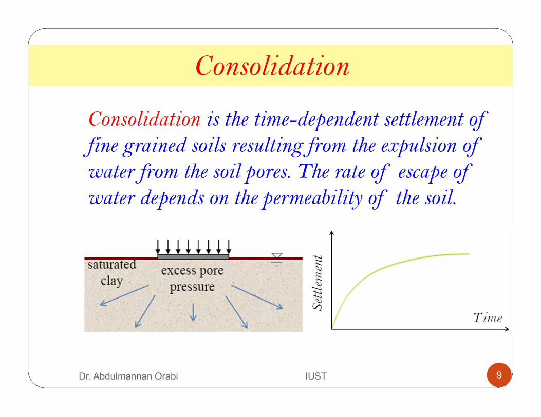
Consolidation is the time-dependent settlement of fine grained soils resulting from the expulsion of water from the soil pores. The rate of escape of water depends on the permeability of the soil.
9Dr. Abdulmannan Orabi IUST
Consolidation
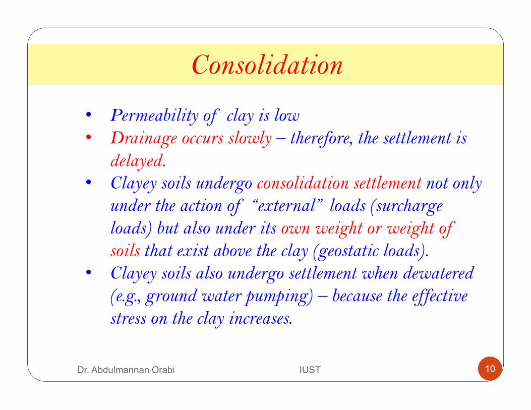
• Permeability of clay is low• Drainage occurs slowly – therefore, the settlement is
delayed.• Clayey soils undergo consolidation settlement not only
under the action of “external” loads (surcharge loads) but also under its own weight or weight of soils that exist above the clay (geostatic loads).
• Clayey soils also undergo settlement when dewatered (e.g., ground water pumping) – because the effective stress on the clay increases.
10Dr. Abdulmannan Orabi IUST
The amount of settlement is proportional to the one-dimensional strain caused by variation in the effective stress. The rate of settlement is a function of the soil type, the geometry of the profile (in 1-D consolidation, the length of the drainage path) and a mathematical solution between a time factor and the percent consolidation which has occurred.
Consolidation
11Dr. Abdulmannan Orabi IUST
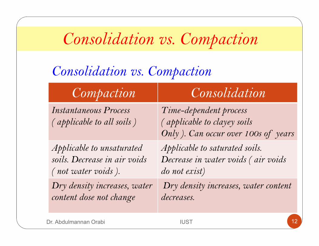
Consolidation vs. Compaction
Compaction ConsolidationInstantaneous Process ( applicable to all soils )
Time-dependent process( applicable to clayey soilsOnly ). Can occur over 100s of years
Applicable to unsaturated soils. Decrease in air voids( not water voids ).
Applicable to saturated soils. Decrease in water voids ( air voids do not exist)
Dry density increases, water content dose not change
Dry density increases, water content decreases.
Consolidation vs. Compaction
12Dr. Abdulmannan Orabi IUST
VoidsVoids
Solids Solids
Before After
�� =���
1 + ���� =
��1 + �
= ∆ℎ
� = ���
��
� � = ����
��
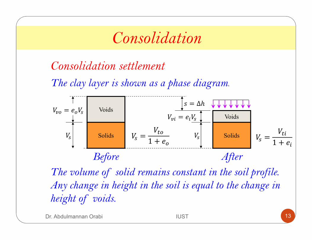
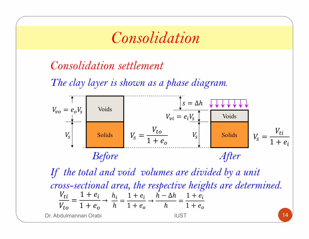
The clay layer is shown as a phase diagram.
The volume of solid remains constant in the soil profile. Any change in height in the soil is equal to the change in height of voids.
Consolidation settlement
Consolidation
13Dr. Abdulmannan Orabi IUST
VoidsVoids
Solids Solids
Before After
�� =���
1 + ���� =
��1 + �
�����
=1 + �1 + ��
= ∆ℎ
� = ���
��
� � = ����
��
Consolidation settlement
The clay layer is shown as a phase diagram.
If the total and void volumes are divided by a unit cross-sectional area, the respective heights are determined.
ℎℎ=1 + �1 + ��
→ℎ − ∆ℎ
ℎ=1 + �1 + ��
→
Consolidation
14Dr. Abdulmannan Orabi IUST
� Consolidation
VoidsVoids
Solids Solids
Before After
Consolidation
�� =���
1 + ���� =
��1 + �
= ∆ℎ
� = ���
��
� � = ����
��
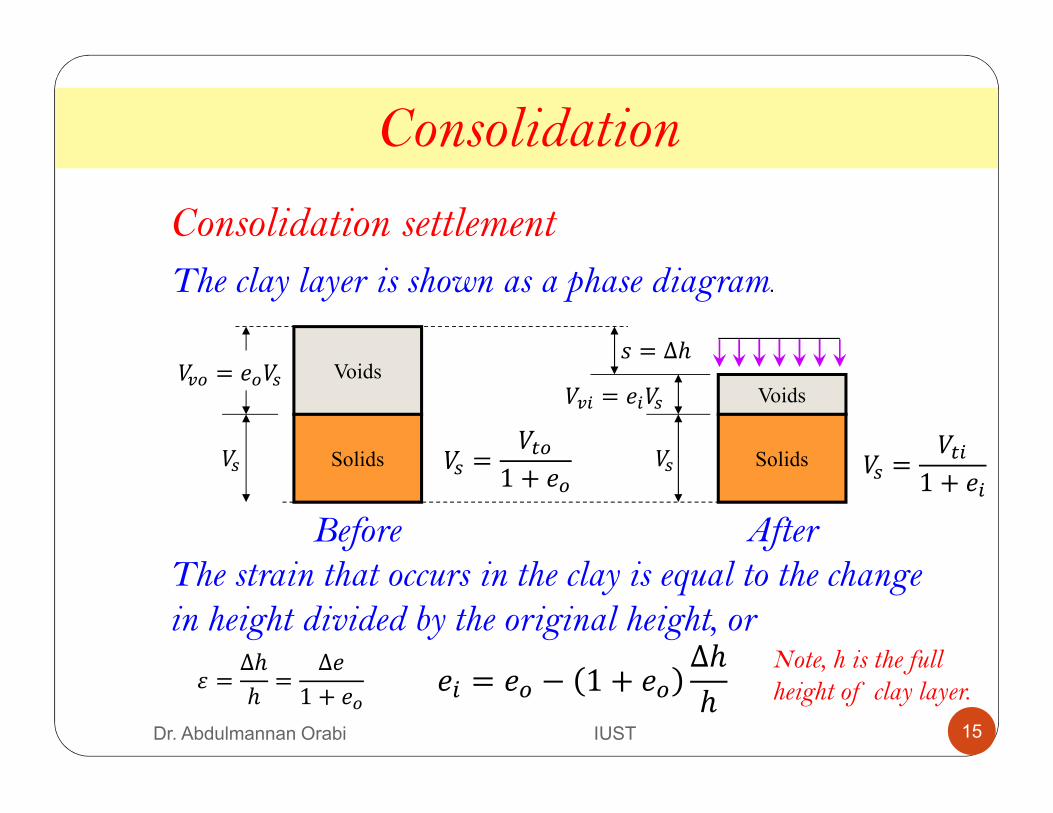
The clay layer is shown as a phase diagram.
� =∆ℎ
ℎ=
∆�
1 + ��
The strain that occurs in the clay is equal to the change in height divided by the original height, or
� = �� − 1 + ��∆ℎ
ℎ
Consolidation settlement
Note, h is the full height of clay layer.
15Dr. Abdulmannan Orabi IUST
During consolidation , remains the same, decreases (due to drainage) while ∆�� increases, transferring the load from water to the soil.
Fundamentals of Consolidation
Spring-cylinder model
∆�∆�
16Dr. Abdulmannan Orabi IUST
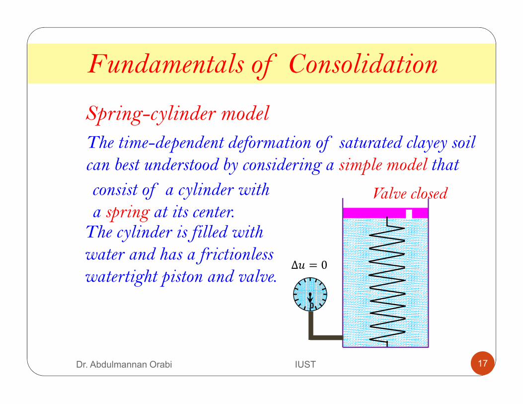
The time-dependent deformation of saturated clayey soil can best understood by considering a simple model that
Fundamentals of Consolidation
0
Valve closed
∆� = 0
The cylinder is filled with water and has a frictionless watertight piston and valve.
Spring-cylinder model
consist of a cylinder with a spring at its center.
17Dr. Abdulmannan Orabi IUST
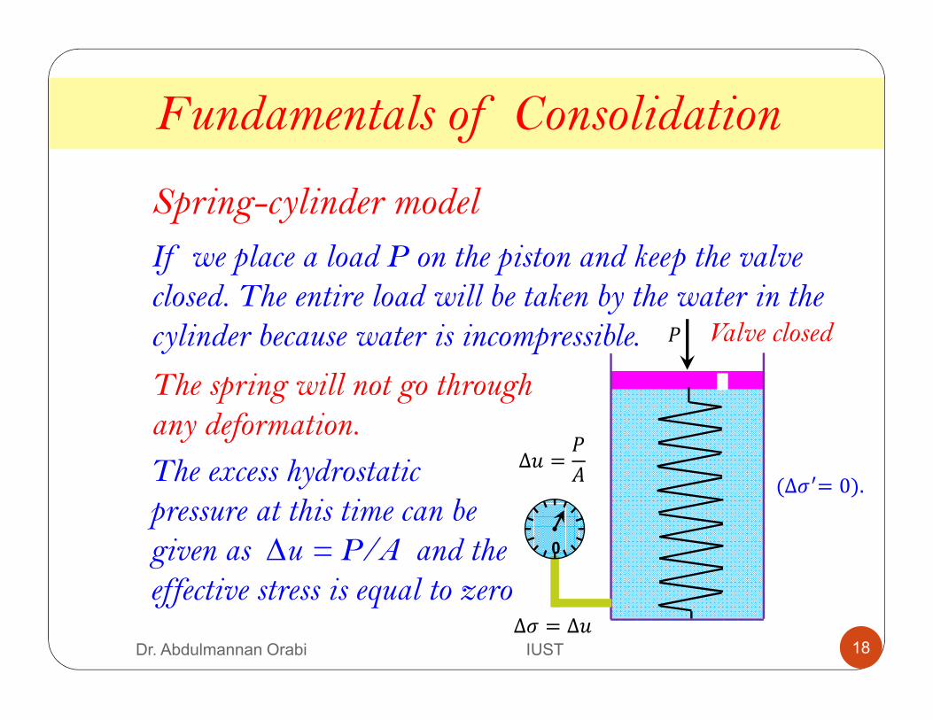
If we place a load P on the piston and keep the valve closed. The entire load will be taken by the water in the cylinder because water is incompressible.
Fundamentals of Consolidation
0
The excess hydrostatic pressure at this time can be given as ∆u = P/A and the effective stress is equal to zero
∆� =�
� (∆��= 0).
∆� = ∆�
Valve closed �
The spring will not go through any deformation.
Spring-cylinder model
18Dr. Abdulmannan Orabi IUST
Fundamentals of Consolidation
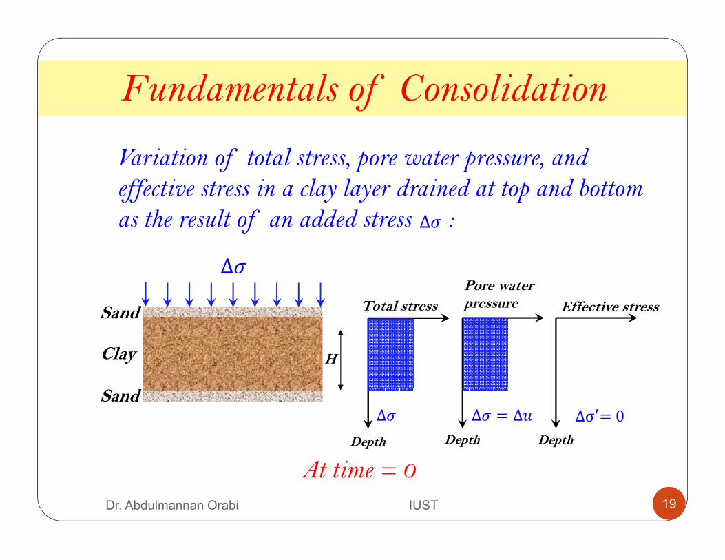
Variation of total stress, pore water pressure, and effective stress in a clay layer drained at top and bottom as the result of an added stress :
Sand
Sand
Clay H
Depth Depth Depth
Effective stress Total stress
Pore water pressure
∆�
∆� ∆σ�= 0∆� = ∆�
At time = 0
∆�
19Dr. Abdulmannan Orabi IUST
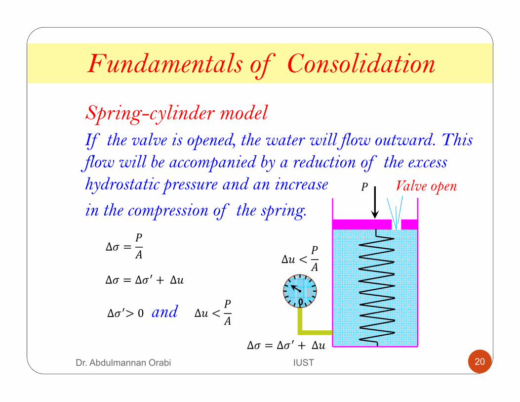
If the valve is opened, the water will flow outward. This flow will be accompanied by a reduction of the excess hydrostatic pressure and an increase
in the compression of the spring.
Fundamentals of Consolidation
0
∆��> 0 and ∆� <�
�
∆� = ∆�� +∆�
�
∆� =�
�
Valve open
∆� <�
�
∆� = ∆�� +∆�
Spring-cylinder model
20Dr. Abdulmannan Orabi IUST
Fundamentals of Consolidation
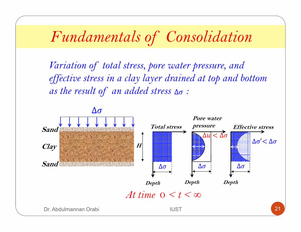
Variation of total stress, pore water pressure, and effective stress in a clay layer drained at top and bottom as the result of an added stress :
Sand
Sand
Clay H
Depth Depth Depth
Effective stress Total stress
Pore water pressure
∆�
∆� ∆�
At time 0 ˂ t ˂ ∞
∆� < ∆�∆σ�<∆�
∆�
∆�
21Dr. Abdulmannan Orabi IUST
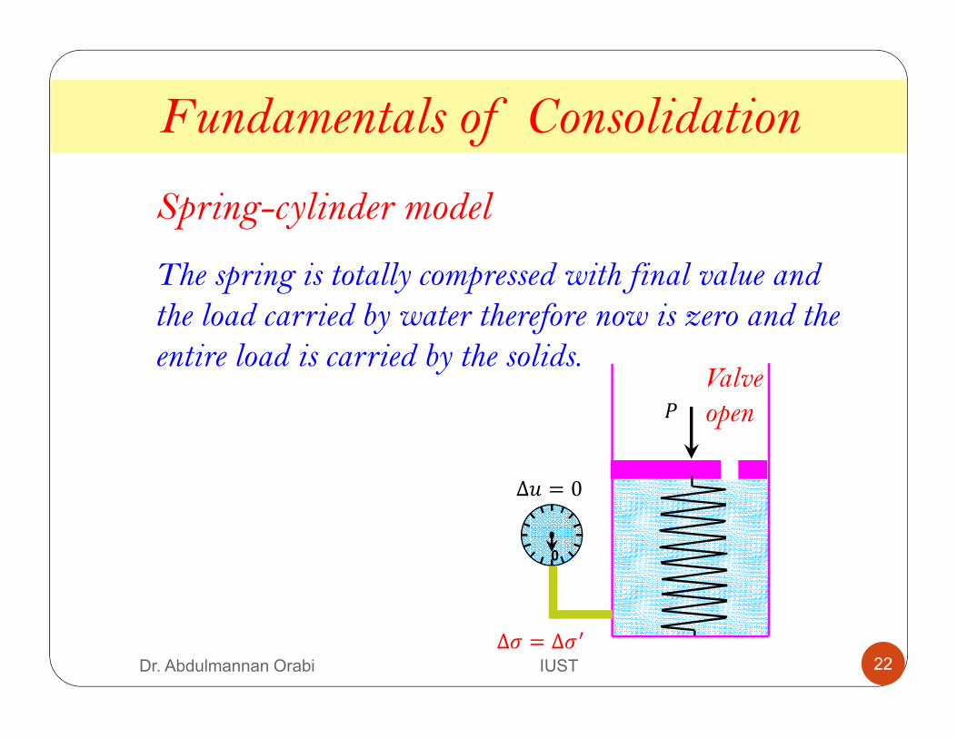
Fundamentals of Consolidation
0
∆� = 0
�
Valve open
∆� = ∆��
Spring-cylinder model
The spring is totally compressed with final value and the load carried by water therefore now is zero and the entire load is carried by the solids.
22Dr. Abdulmannan Orabi IUST
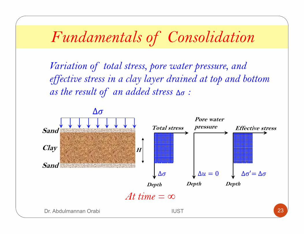
Fundamentals of Consolidation
Variation of total stress, pore water pressure, and effective stress in a clay layer drained at top and bottom as the result of an added stress :
Sand
Sand
Clay H
Depth Depth Depth
Effective stress Total stress
Pore water pressure
∆�
∆� ∆σ�= ∆�∆� = 0
At time = ∞
∆�
23Dr. Abdulmannan Orabi IUST
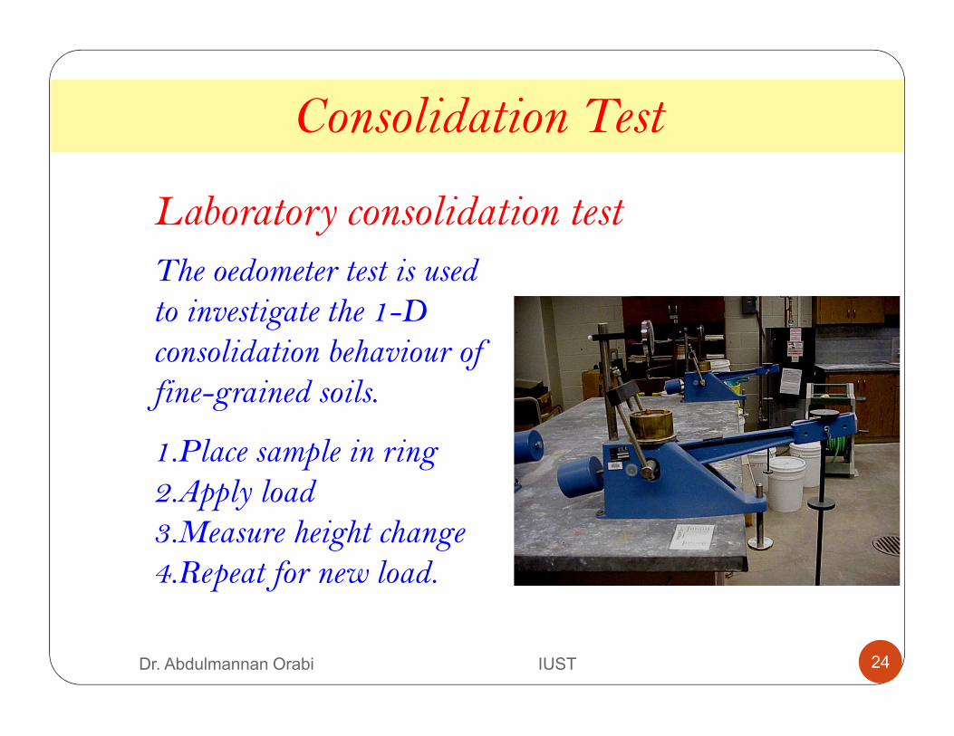
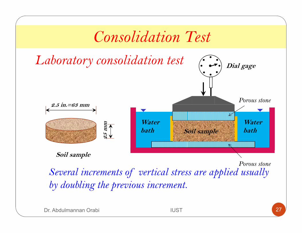
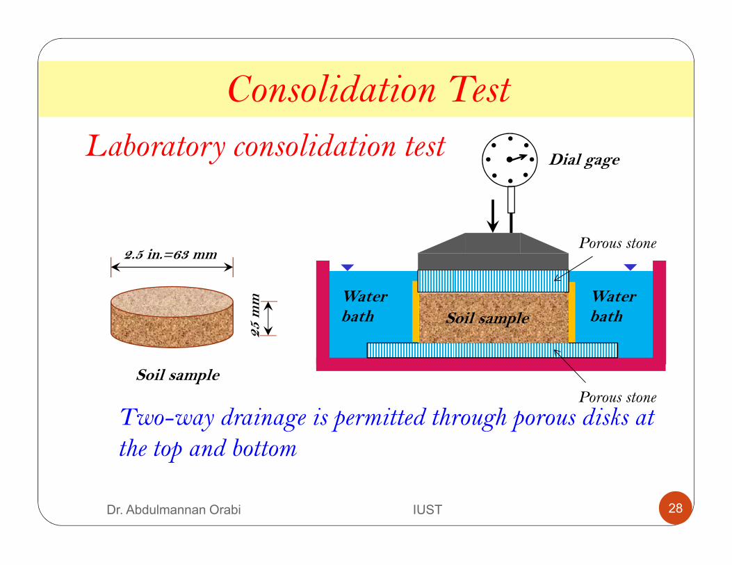
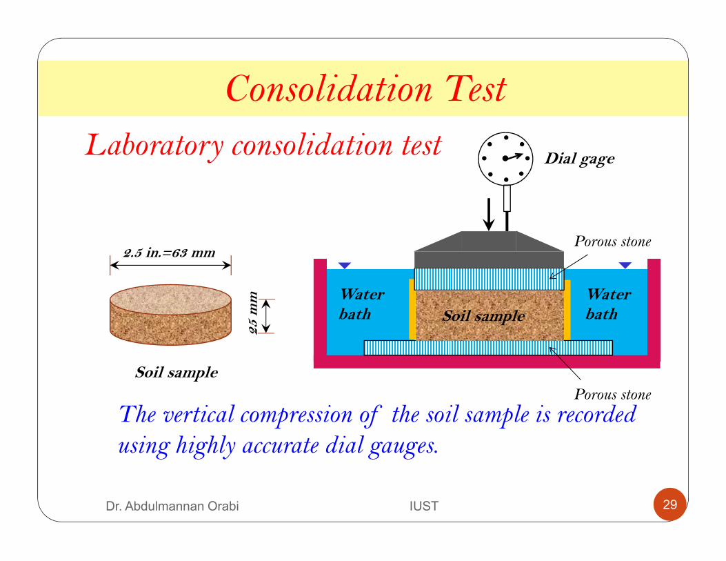
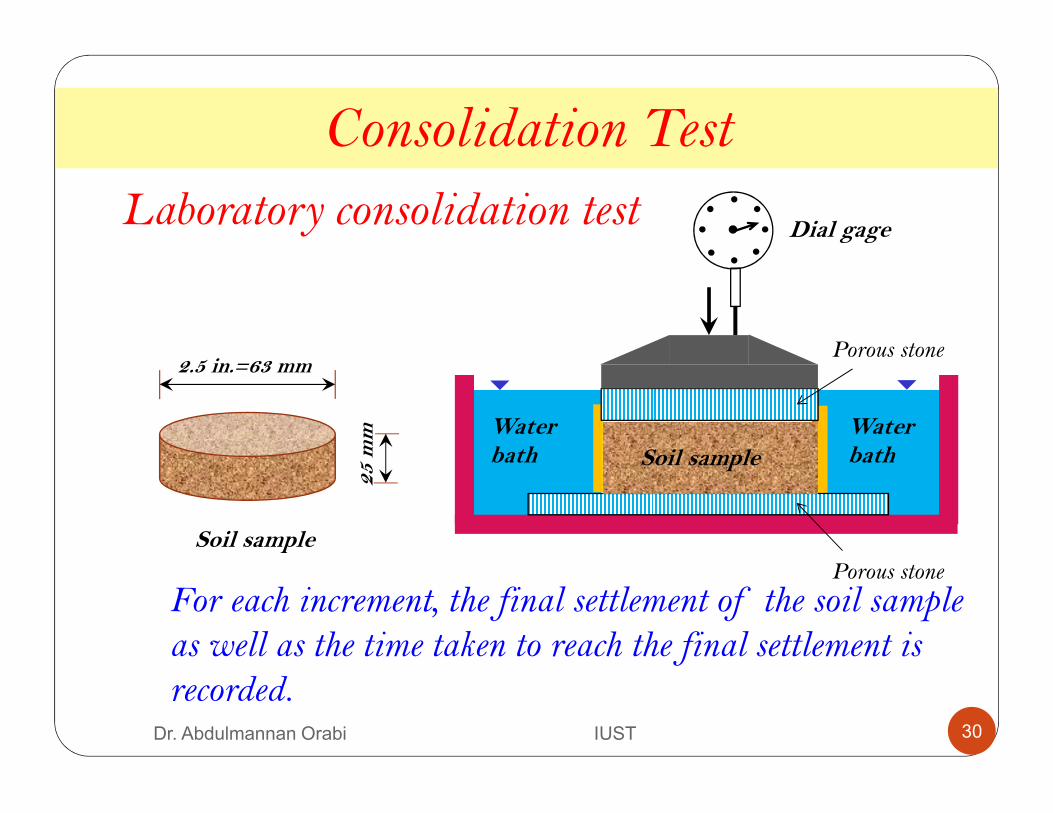
Laboratory consolidation test
Consolidation Test
1.Place sample in ring 2.Apply load 3.Measure height change 4.Repeat for new load.
The oedometer test is used to investigate the 1-D consolidation behaviour of fine-grained soils.
24Dr. Abdulmannan Orabi IUST
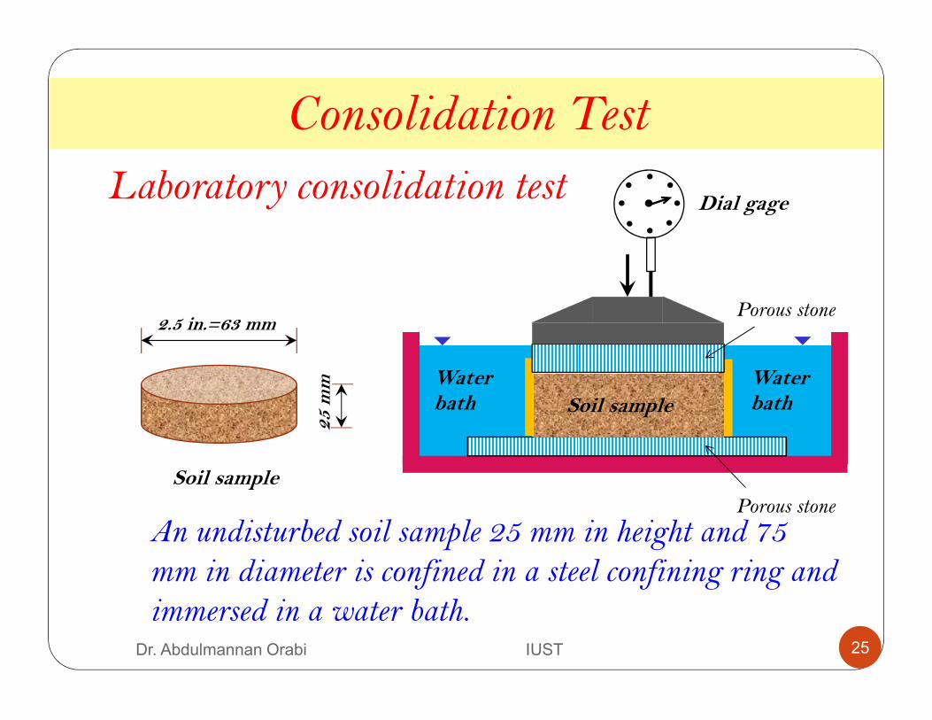
Consolidation Test
Soil sample
Dial gage
Porous stone
Porous stone
Water bath
Water bath
Laboratory consolidation test
Soil sample
25
mm
2.5 in.=63 mm
An undisturbed soil sample 25 mm in height and 75 mm in diameter is confined in a steel confining ring and immersed in a water bath.
25Dr. Abdulmannan Orabi IUST

Consolidation Test
Soil sample
Dial gage
Porous stone
Porous stone
Water bath
Water bath
Laboratory consolidation test
Soil sample
25
mm
2.5 in.=63 mm
It is subjected to a compressive stress by applying a vertical load, which is assumed to act uniformly over the area of the soil sample.
26Dr. Abdulmannan Orabi IUST
Consolidation Test
Soil sample
Dial gage
Porous stone
Porous stone
Water bath
Water bath
Laboratory consolidation test
Soil sample
25
mm
2.5 in.=63 mm
Several increments of vertical stress are applied usually by doubling the previous increment.
27Dr. Abdulmannan Orabi IUST
Consolidation Test
Soil sample
Dial gage
Porous stone
Porous stone
Water bath
Water bath
Laboratory consolidation test
Soil sample
25
mm
2.5 in.=63 mm
Two-way drainage is permitted through porous disks at the top and bottom
28Dr. Abdulmannan Orabi IUST
Consolidation Test
Soil sample
Dial gage
Porous stone
Porous stone
Water bath
Water bath
Laboratory consolidation test
Soil sample
25
mm
2.5 in.=63 mm
The vertical compression of the soil sample is recorded using highly accurate dial gauges.
29Dr. Abdulmannan Orabi IUST
Consolidation Test
Soil sample
Dial gage
Porous stone
Porous stone
Water bath
Water bath
Laboratory consolidation test
Soil sample
25
mm
2.5 in.=63 mm
For each increment, the final settlement of the soil sample as well as the time taken to reach the final settlement is recorded.
30Dr. Abdulmannan Orabi IUST
Consolidation Test
Laboratory consolidation test
Soil sample
25
mm
2.5 in.=63 mm
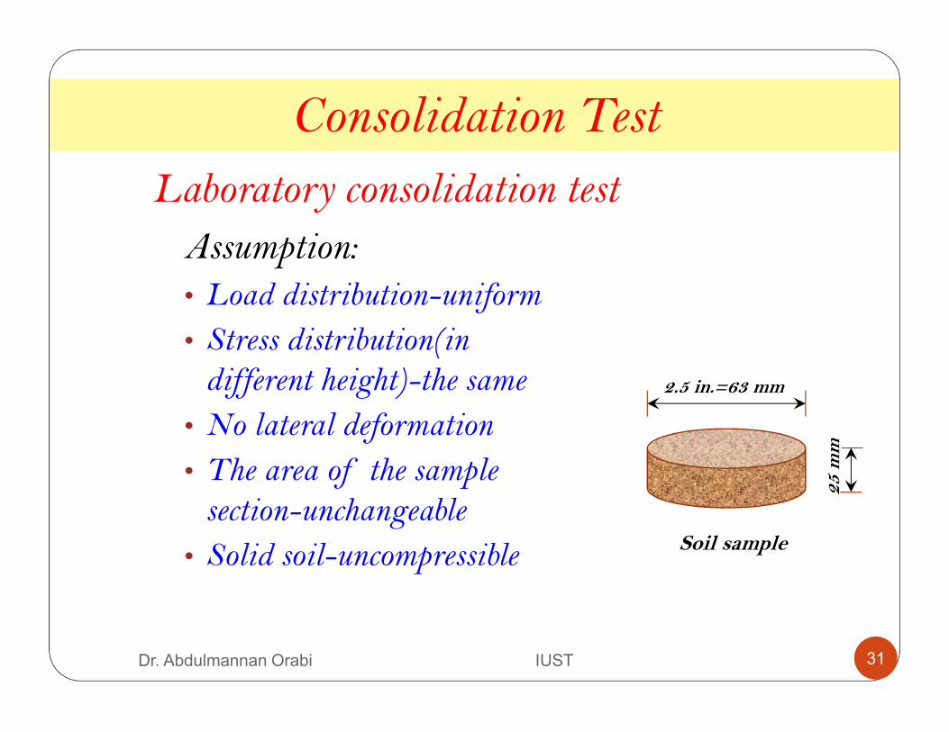
Assumption:
• Load distribution-uniform
• Stress distribution(in different height)-the same
• No lateral deformation
• The area of the sample section-unchangeable
• Solid soil-uncompressible
31Dr. Abdulmannan Orabi IUST
A laboratory consolidation test is performed on an undisturbed sample of a cohesive soil to determine its compressibility characteristics. The soil sample is assumed to be representing a soil layer in the ground.
A conventional consolidation test is conducted over a number of load increments. The number of load increments should cover the stress range from the initial stress state of the soil to the final stress state the soil layer is expected to experience due to the proposed construction.
Laboratory consolidation test
Consolidation Test
32Dr. Abdulmannan Orabi IUST
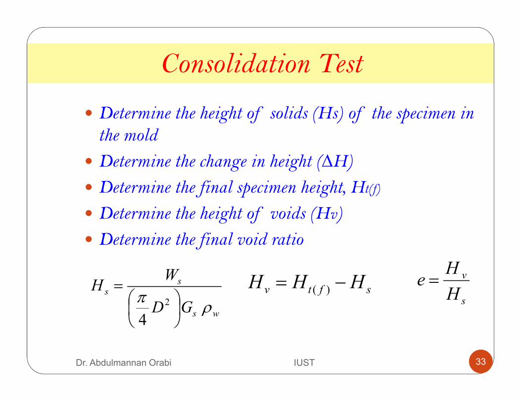
� Determine the height of solids (Hs) of the specimen in the mold
� Determine the change in height (∆H)
� Determine the final specimen height, Ht(f)
� Determine the height of voids (Hv)
� Determine the final void ratio
ws
ss
GD
WH
ρπ
=
2
4
sftv HHH −= )(s
v
H
He =
Consolidation Test
33Dr. Abdulmannan Orabi IUST

The effective stress σ’ and the corresponding void ratios e at the end of consolidation are plotted on semi-logarithmic graph:
In the initial phase, relatively great change in pressure only results in less change in void ratio e. The reason is part of the pressure got to compensate the expansion when the soil specimen was sampled. In the following phase e changes at a great rate
Consolidation Test
34Dr. Abdulmannan Orabi IUST
Consolidation Test
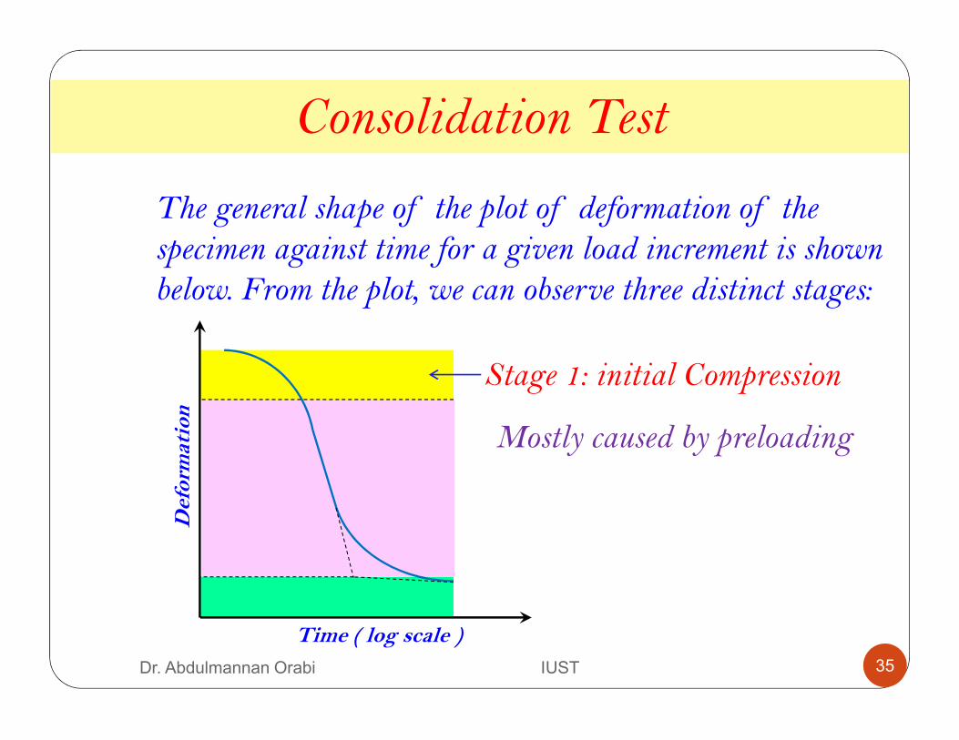
The general shape of the plot of deformation of the specimen against time for a given load increment is shown below. From the plot, we can observe three distinct stages:
Time ( log scale )
Def
orm
atio
n
Stage 1: initial Compression
Mostly caused by preloading
35Dr. Abdulmannan Orabi IUST
Consolidation Test
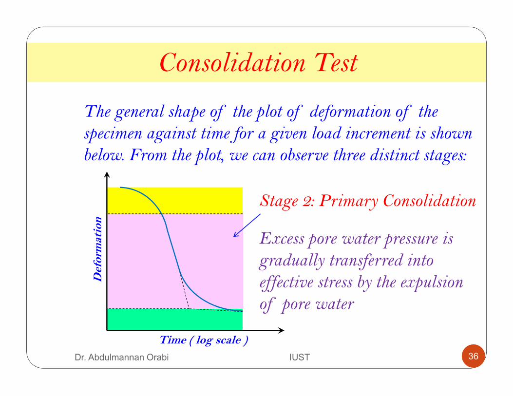
The general shape of the plot of deformation of the specimen against time for a given load increment is shown below. From the plot, we can observe three distinct stages:
Time ( log scale )
Def
orm
atio
n
Stage 2: Primary Consolidation
Excess pore water pressure is gradually transferred into effective stress by the expulsion of pore water
36Dr. Abdulmannan Orabi IUST
Consolidation Test
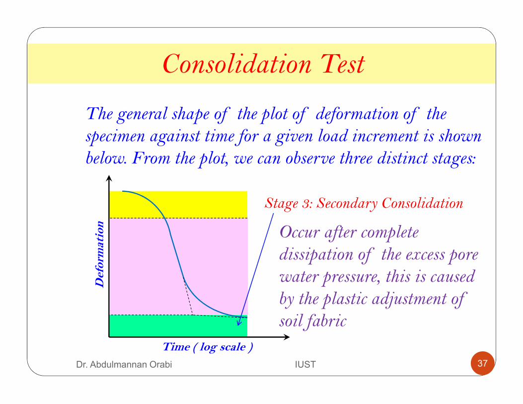
The general shape of the plot of deformation of the specimen against time for a given load increment is shown below. From the plot, we can observe three distinct stages:
Time ( log scale )
Def
orm
atio
n
Stage 3: Secondary Consolidation
Occur after complete dissipation of the excess pore water pressure, this is caused by the plastic adjustment of soil fabric
37Dr. Abdulmannan Orabi IUST
Increments in a conventional consolidation test are generally of 24 hr. duration and the load is doubled in the successive increment.
Laboratory consolidation test
Consolidation Test
The main purpose of consolidation tests is to obtain soil data which is used in predicting the rate and amount of settlement of structures founded on clay.
38Dr. Abdulmannan Orabi IUST
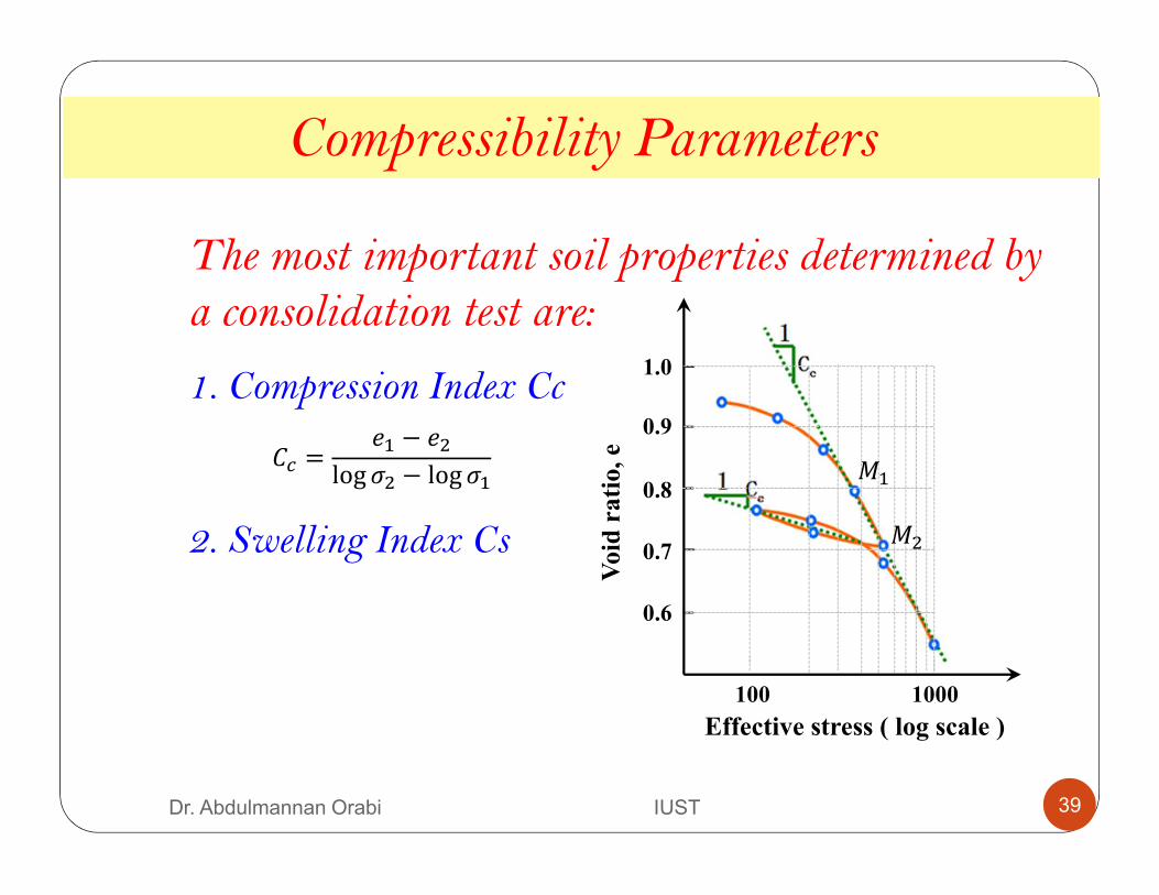
The most important soil properties determined by a consolidation test are:
Compressibility Parameters
100 1000
0.9
0.8
0.7
0.6
1.0
Effective stress ( log scale )
Void
rati
o, e�� =
� − �!log �! − log� %
%!
1. Compression Index Cc
2. Swelling Index Cs
39Dr. Abdulmannan Orabi IUST
Compressibility Parameters
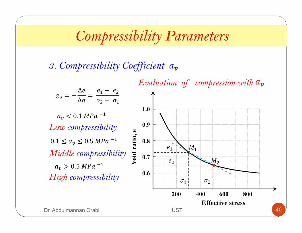
3. Compressibility Coefficient
0.9
0.8
0.7
0.6
1.0
Effective stress
Void
rati
o, e
200 400 600 800
%
%!
�
�!
�!�
& = −∆�
∆�=
� −�!�! −�
Evaluation of compression with &
& < 0.1%�&'
Low compressibility
0.1 ≤ & ≤ 0.5%�&'
Middle compressibility
& > 0.5%�&'
High compressibility
&
40Dr. Abdulmannan Orabi IUST

Compressibility Parameters
4. Coefficient of volume compressibility mv
0.9
0.8
0.7
0.6
1.0
Effective stress
Void ratio, e
200 400 600 800
%
%!
�
�!
�!�
* =&
1 + ��
This parameter is defined as change in volume per unit volume as a ratio with respect to the change in stress.
41Dr. Abdulmannan Orabi IUST
Compressibility Parameters
5. Preconsolidation Pressure
Normally consolidated clay, whose present effective overburden pressure is the maximum pressure that the soil was subjected to in the past. Overconsolidated, whose present effective overburden pressure is less than that which the soil experienced in the past. The maximum effective past pressure is called the preconsolidation pressure.
42Dr. Abdulmannan Orabi IUST
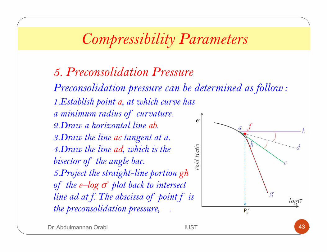
5. Preconsolidation Pressure
Compressibility Parameters
Preconsolidation pressure can be determined as follow :1.Establish point a, at which curve has a minimum radius of curvature. 2.Draw a horizontal line ab. 3.Draw the line ac tangent at a. 4.Draw the line ad, which is the bisector of the angle bac. 5.Project the straight-line portion gh
of the e–log σ’ plot back to intersect line ad at f. The abscissa of point f is the preconsolidation pressure, .
43Dr. Abdulmannan Orabi IUST

The OCR for an OC soil is greater than 1.
Most OC soils have fairly high shear strength.
The OCR cannot have a value less than 1.
Compressibility Parameters
5. Preconsolidation Pressure
The overconsolidation ratio (OCR) for a soil can now be defined as
+�, = ���
���
where :
��� = preconsolidation pressure
��� = present effective vertical pressure
44Dr. Abdulmannan Orabi IUST
The coefficient of consolidation ( ) can be determined by the (Casagrande) Logarithm-of-Time and by (Taylor) Square –Root of Time Methods.
-
The rate of consolidation settlement is estimated using the Coefficient of consolidation Cv. This parameter is determined for each load increment in the test.
Compressibility Parameters
6. Coefficient of consolidation Cv
45Dr. Abdulmannan Orabi IUST
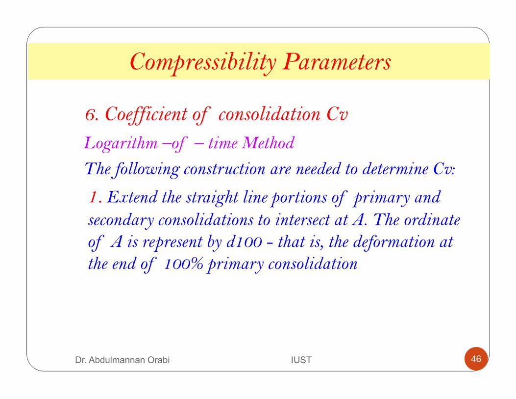
Logarithm –of – time Method
The following construction are needed to determine Cv:
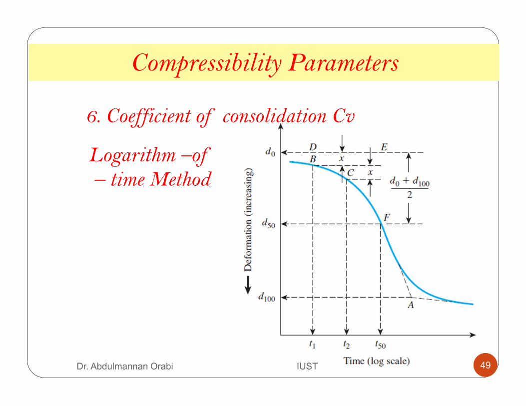
1. Extend the straight line portions of primary and
secondary consolidations to intersect at A. The ordinate of A is represent by d100 - that is, the deformation at the end of 100% primary consolidation
Compressibility Parameters
6. Coefficient of consolidation Cv
46Dr. Abdulmannan Orabi IUST
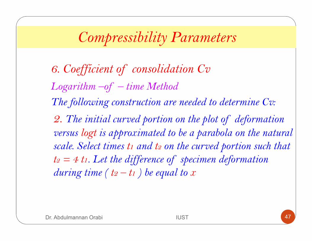
Logarithm –of – time Method
The following construction are needed to determine Cv:
2. The initial curved portion on the plot of deformation
versus logt is approximated to be a parabola on the natural scale. Select times t1 and t2 on the curved portion such that t2 = 4 t1. Let the difference of specimen deformation during time ( t2 – t1 ) be equal to x
6. Coefficient of consolidation Cv
Compressibility Parameters
47Dr. Abdulmannan Orabi IUST
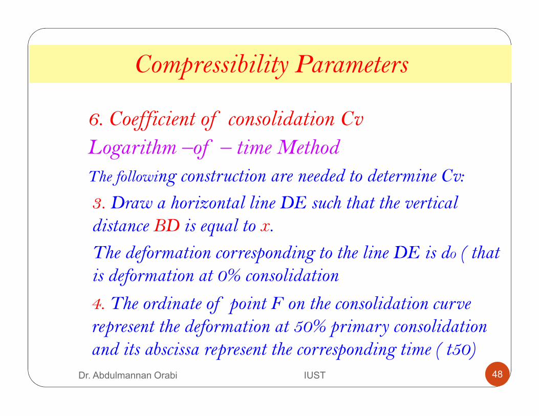
Logarithm –of – time Method
The following construction are needed to determine Cv:
3. Draw a horizontal line DE such that the vertical distance BD is equal to x.
The deformation corresponding to the line DE is d0 ( that is deformation at 0% consolidation
4. The ordinate of point F on the consolidation curve represent the deformation at 50% primary consolidation and its abscissa represent the corresponding time ( t50)
6. Coefficient of consolidation Cv
Compressibility Parameters
48Dr. Abdulmannan Orabi IUST
Logarithm –of– time Method
6. Coefficient of consolidation Cv
Compressibility Parameters
49Dr. Abdulmannan Orabi IUST
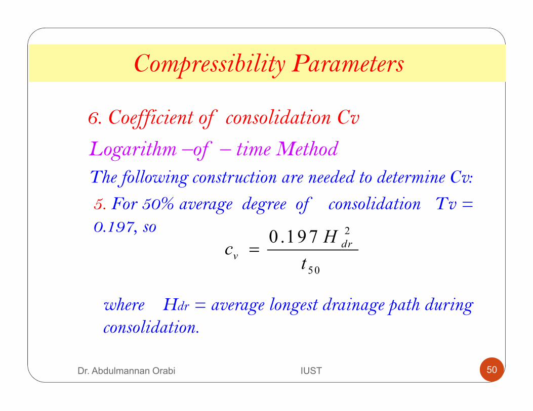
Logarithm –of – time Method
The following construction are needed to determine Cv:
5. For 50% average degree of consolidation Tv = 0.197, so 2
50
0.197 drv
Hc
t=
where Hdr = average longest drainage path during consolidation.
6. Coefficient of consolidation Cv
Compressibility Parameters
50Dr. Abdulmannan Orabi IUST
Logarithm –of – time Method
The following construction are needed to determine Cv:
For specimen drained at both top and bottom, Hdr
equals one-half the overage height of the specimen during consolidation .
For specimen drained on only one side, Hdr equals the average height of the specimen during consolidation.
6. Coefficient of consolidation Cv
Compressibility Parameters
51Dr. Abdulmannan Orabi IUST
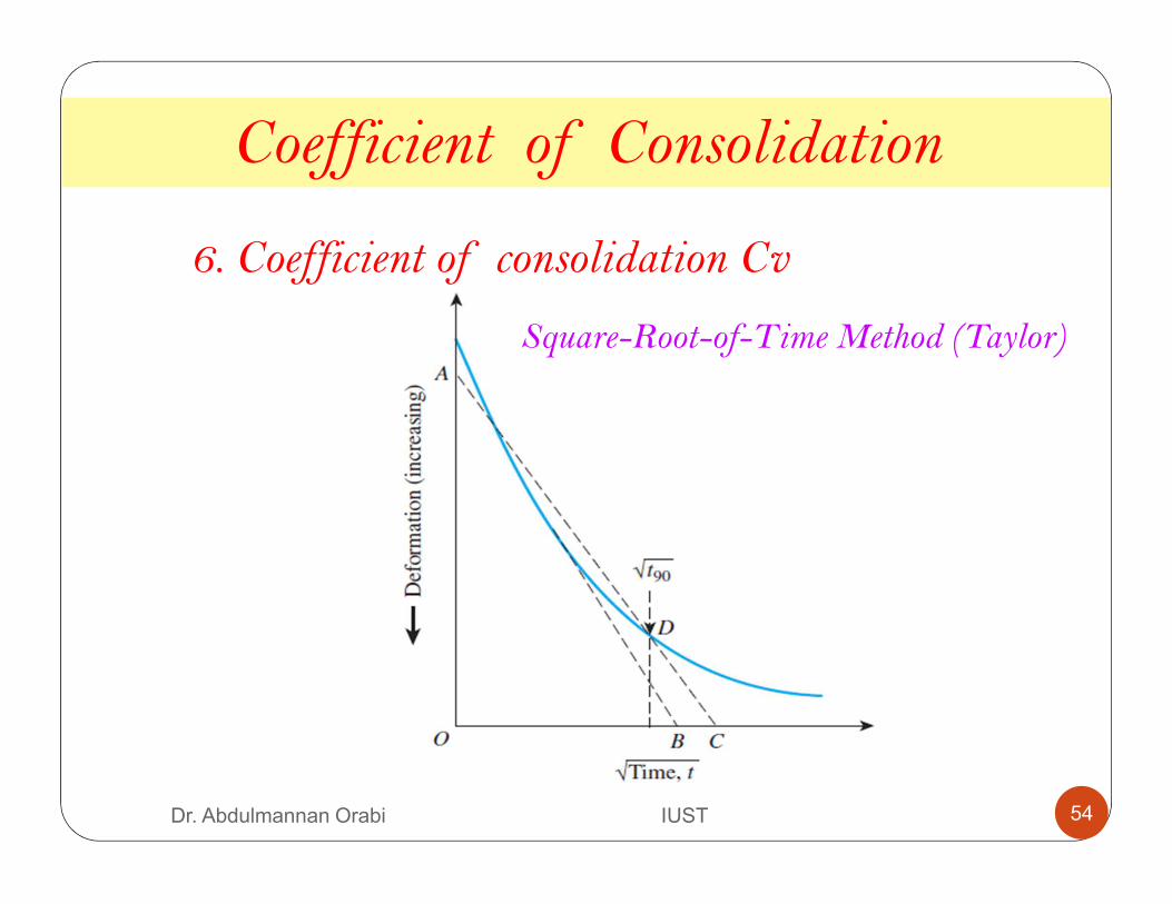
Square-Root-of-Time Method (Taylor)
Plot a deformation against the square root of time
1. Draw a line AB through the early portion of the curve
2. Draw a line AC such that OC = 1.15 OB.
The abscissa of point D, which is the intersection of AC and the consolidation curve, gives the square root of time for 90% consolidation
Compressibility Parameters
6. Coefficient of consolidation Cv
52Dr. Abdulmannan Orabi IUST
Square-Root-of-Time Method (Taylor)
Plot a deformation against the square root of time
3. For 90% consolidation T90 = 0.848, so
Coefficient of Consolidation
2
90
0.848 drv
Hc
t=
6. Coefficient of consolidation Cv
53Dr. Abdulmannan Orabi IUST
Coefficient of Consolidation
Square-Root-of-Time Method (Taylor)
6. Coefficient of consolidation Cv
54Dr. Abdulmannan Orabi IUST
Consolidated Settlement
. =-� ℎ
1 + ��/01
� �� +∆� � ��
. =-�ℎ
1 + ��/01
� �� +∆� � ��
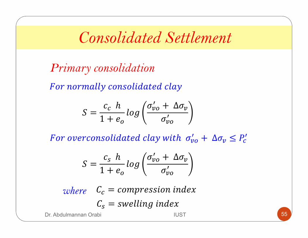
203403*&//5-040/67&8�7-/&5
20309�3-040/67&8�7-/&5:68ℎ� �� +∆� ≤ ��
�
Primary consolidation
�� = -0*;3�604647�<
�� = :�//641647�<where
55Dr. Abdulmannan Orabi IUST
. =-�ℎ
1 + ��/01
���
� �� +
-� ℎ
1 + ��/01
� �� +∆� ���
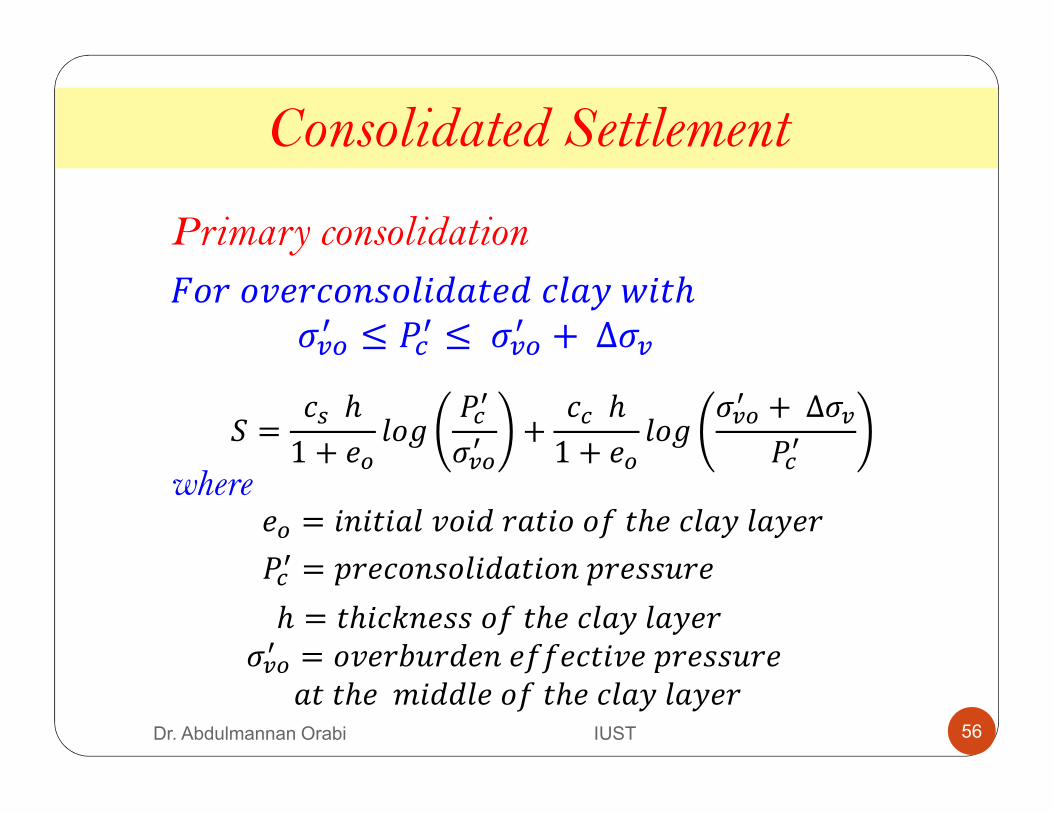
��� = ;3�-040/67&8604;3��3�
�� = 64686&/90673&8600=8ℎ�-/&5/&5�3
ℎ = 8ℎ6->4�0=8ℎ�-/&5/&5�3� �� = 09�3?�37�4�==�-869�;3��3�&88ℎ�*677/�0=8ℎ�-/&5/&5�3
20309�3-040/67&8�7-/&5:68ℎ� �
� ≤ ��� ≤� �
� +∆�
where
Consolidated Settlement
Primary consolidation
56Dr. Abdulmannan Orabi IUST
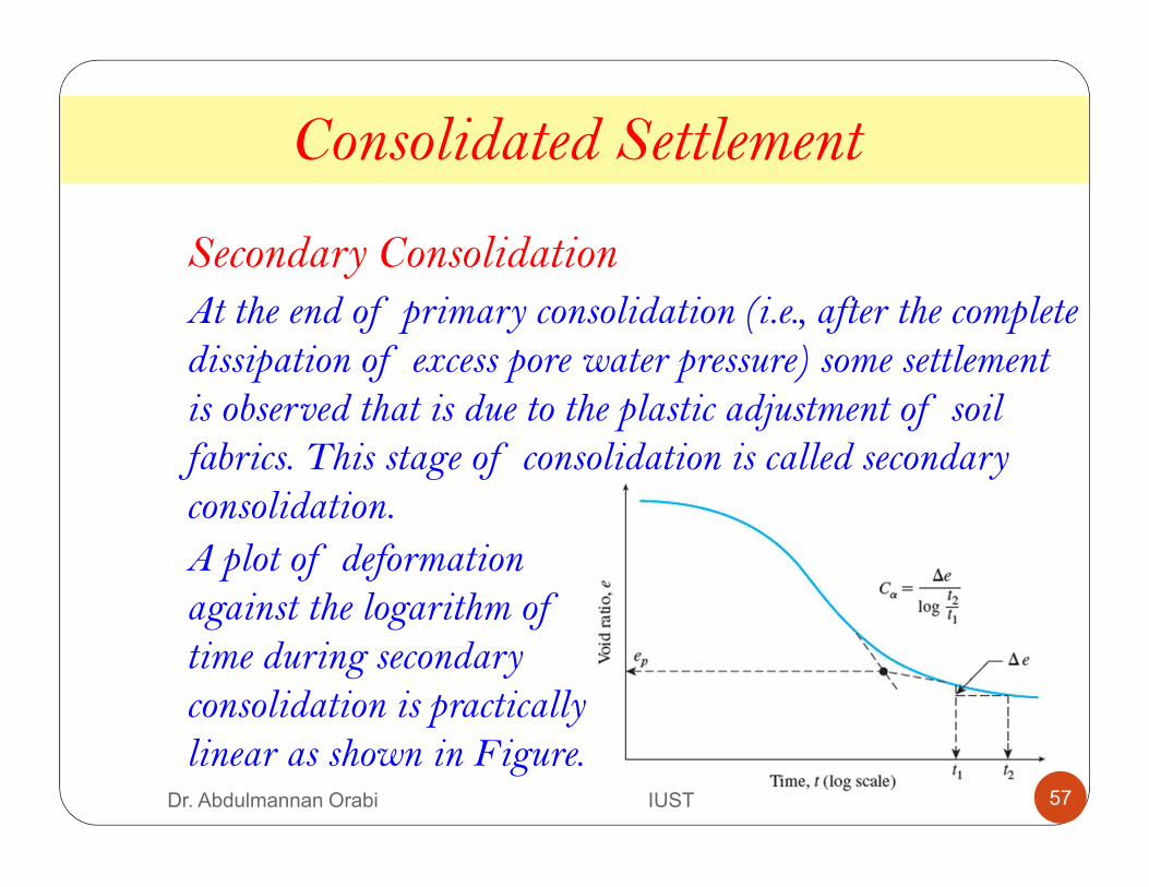
Secondary Consolidation
At the end of primary consolidation (i.e., after the complete dissipation of excess pore water pressure) some settlement is observed that is due to the plastic adjustment of soil fabrics. This stage of consolidation is called secondary consolidation.
Consolidated Settlement
A plot of deformation against the logarithm of time during secondary consolidation is practically linear as shown in Figure.
57Dr. Abdulmannan Orabi IUST
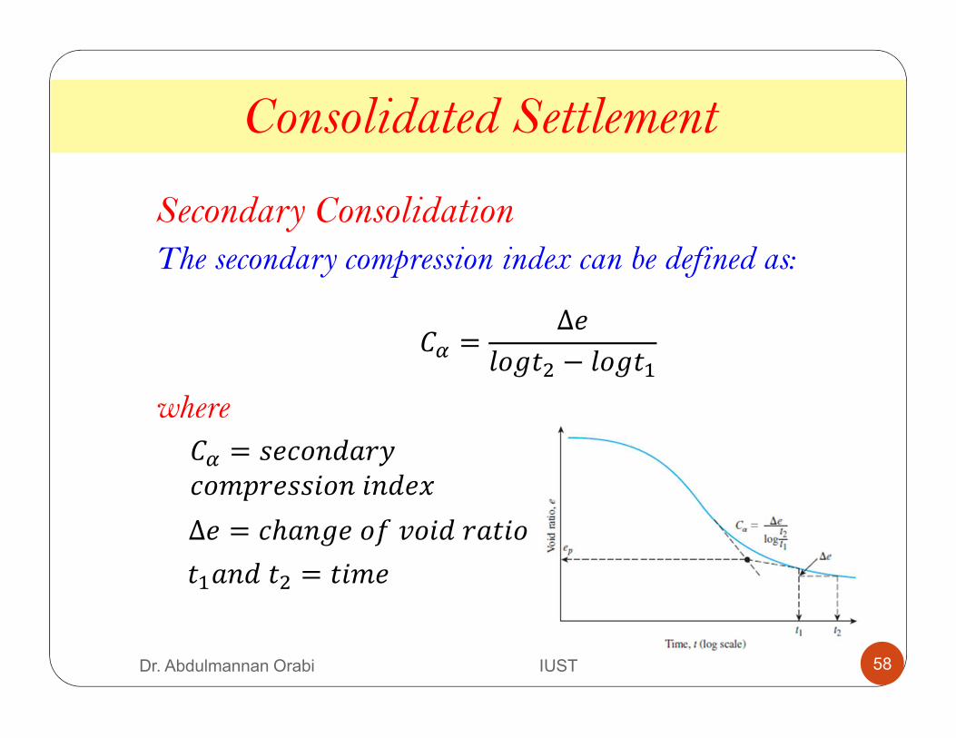
Secondary Consolidation
The secondary compression index can be defined as:
Consolidated Settlement
�@ =∆�
/018! − /018
where
�@ = �-047&35-0*;3�604647�<
∆� = -ℎ&41�0=90673&860
8 &478! = 86*�
58Dr. Abdulmannan Orabi IUST
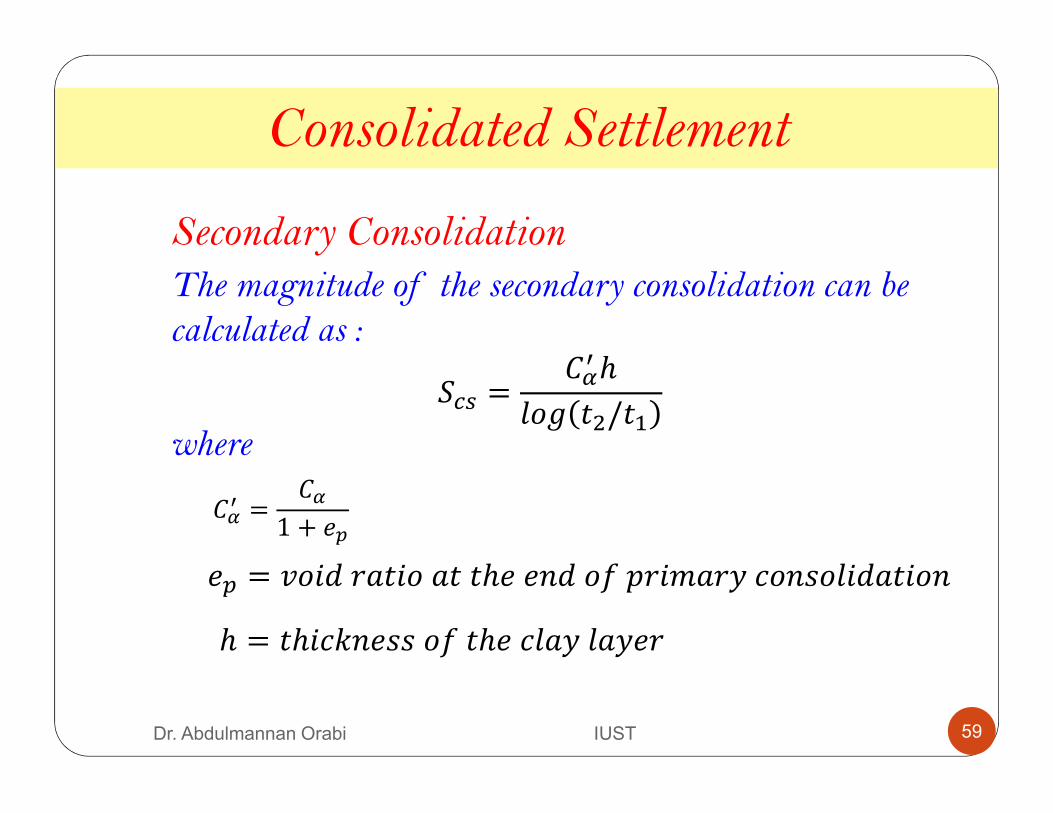
Secondary Consolidation
The magnitude of the secondary consolidation can be calculated as :
Consolidated Settlement
.�� =�@� ℎ
/01 8!/8 where
�@� =
�@1 + �B
�B = 90673&860&88ℎ��470=;36*&35-040/67&8604
ℎ = 8ℎ6->4�0=8ℎ�-/&5/&5�3
59Dr. Abdulmannan Orabi IUST
Secondary Consolidation
Consolidated Settlement
Secondary consolidation settlement is more important in the case of all organic and highly compressible inorganic soils. In overconsolidated inorganic clays, the secondary compression index is very small and of less practical significance.
60Dr. Abdulmannan Orabi IUST

Time Rate of Consolidation
Terzaghi(1925) derived the time rate of consolidation based on the following assumptions:
� 1 The soil is homogeneous and fully saturated.� 2 There is a unique relationship, independent of time,
between void ratio and effective stress.� 3 The solid particles and water are incompressible.� 4 Compression and flow are one-dimensional (vertical).� 5 Strains in the soil are relatively small.� 6 Darcy’s law is valid at all hydraulic gradients.� 7 The coefficient of permeability and volume
compressibility remain constant throughout the process .
61Dr. Abdulmannan Orabi IUST

Time Rate of Consolidation
where
The average degree of consolidation for the entire depth of the clay layer at any time t can be expressed as
C =.�.D
= 1 −
12FGH
I �J7K!LMN
O
��
C = &9�3&1�7�13��0=-040/67&8604
.� = �88/�*�480=8ℎ�/&5�3&886*�8
.D = =64&/�88/�*�480=8ℎ�/&5�3=30*;36*&35-040/67&8604
Degree of consolidation
62Dr. Abdulmannan Orabi IUST
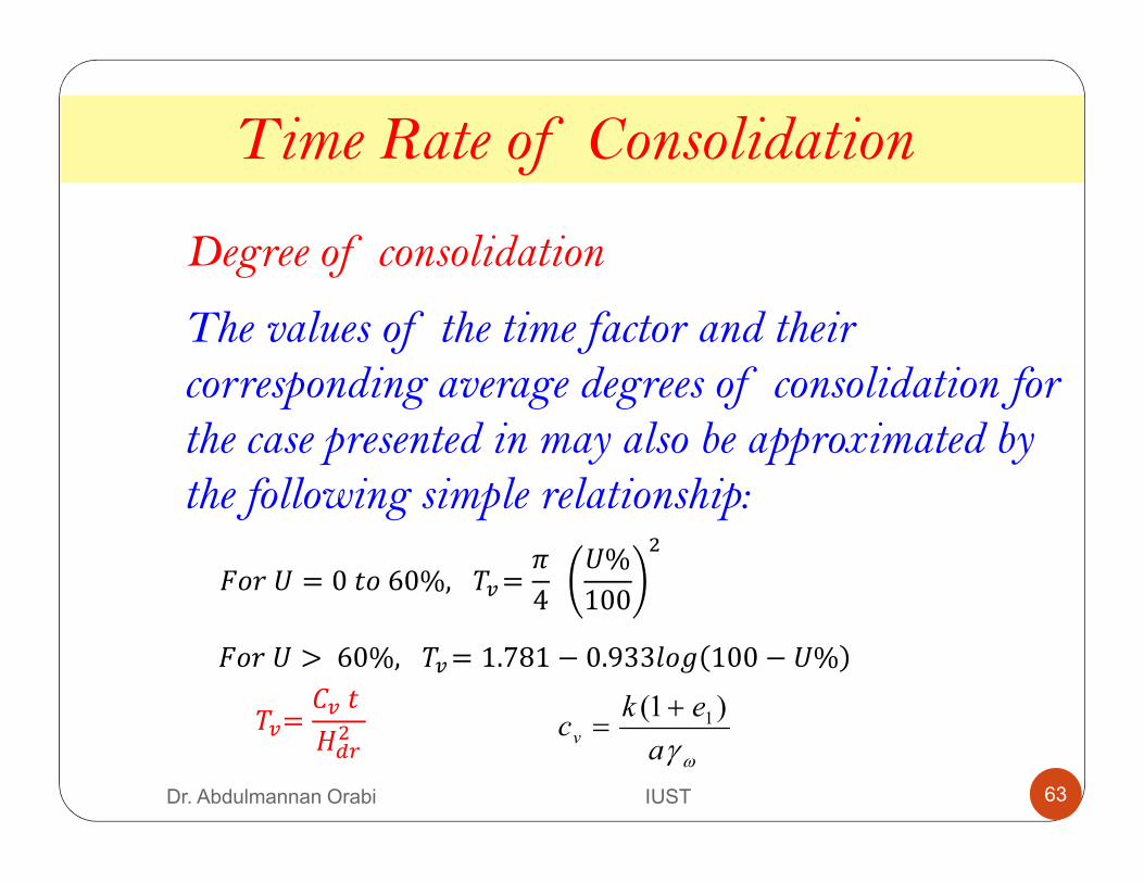
Time Rate of Consolidation
Degree of consolidation
The values of the time factor and their corresponding average degrees of consolidation for the case presented in may also be approximated by the following simple relationship:
203C = 08060%,S =T
4C%
100
!
203C > 60%,S = 1.781 − 0.933/01 100 − C%
S =� 8
FGH!
ωγaek
cv)1( 1+
=
63Dr. Abdulmannan Orabi IUST
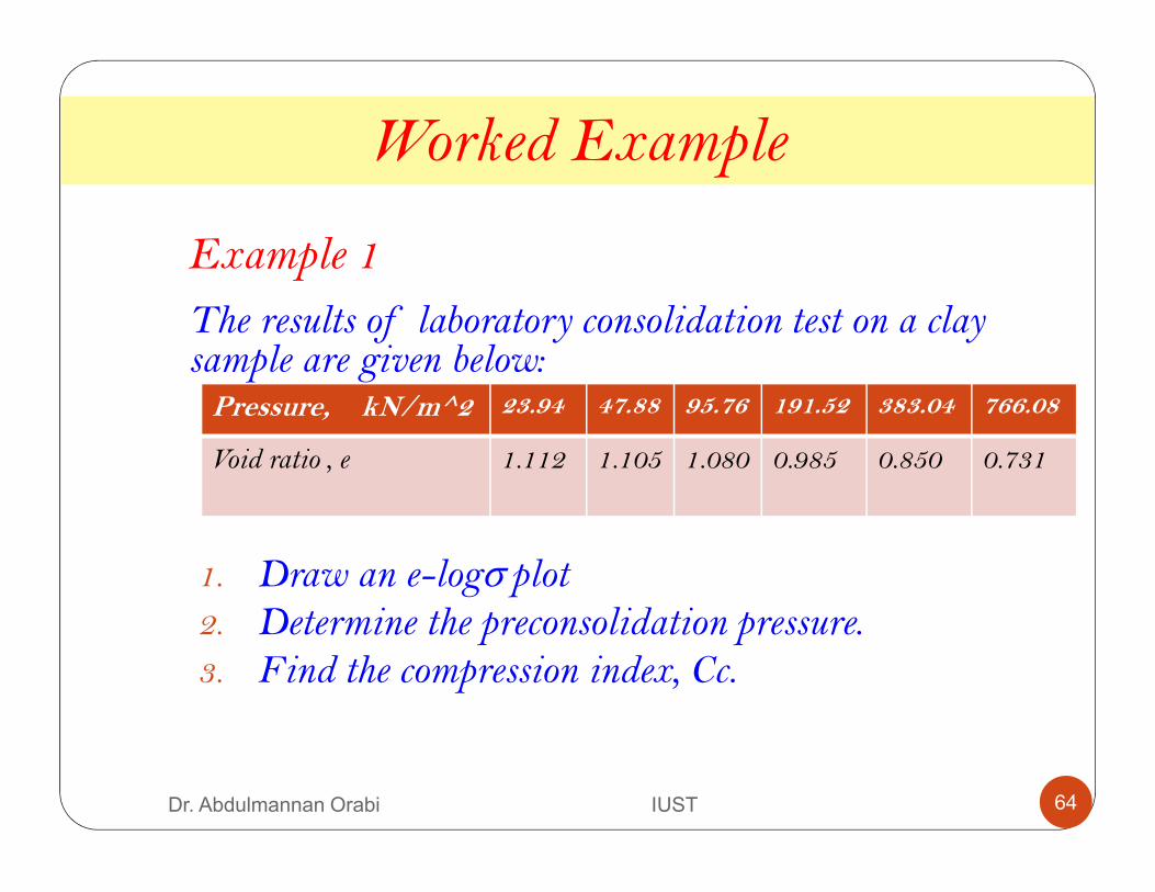
The results of laboratory consolidation test on a clay sample are given below:
1. Draw an e-logσ plot 2. Determine the preconsolidation pressure. 3. Find the compression index, Cc.
Pressure, kN/m^2 23.94 47.88 95.76 191.52 383.04 766.08
Void ratio , e 1.112 1.105 1.080 0.985 0.850 0.731
Worked Example
Example 1
64Dr. Abdulmannan Orabi IUST
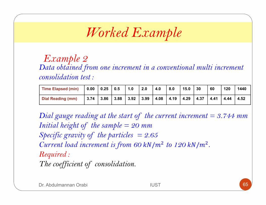
Data obtained from one increment in a conventional multi increment consolidation test :
Dial gauge reading at the start of the current increment = 3.744 mmInitial height of the sample = 20 mmSpecific gravity of the particles = 2.65 Current load increment is from 60 >Z/*! to 120 >Z/*!.Required : The coefficient of consolidation.
Worked Example
Example 2
Time Elapsed (min) 0.00 0.25 0.5 1.0 2.0 4.0 8.0 15.0 30 60 120 1440
Dial Reading (mm) 3.74 3.86 3.88 3.92 3.99 4.08 4.19 4.29 4.37 4.41 4.44 4.52
65Dr. Abdulmannan Orabi IUST
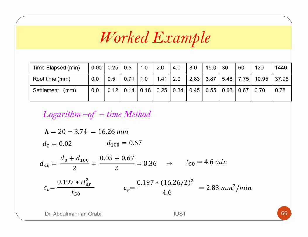
Time Elapsed (min) 0.00 0.25 0.5 1.0 2.0 4.0 8.0 15.0 30 60 120 1440
Root time (mm) 0.0 0.5 0.71 1.0 1.41 2.0 2.83 3.87 5.48 7.75 10.95 37.95
Settlement (mm) 0.0 0.12 0.14 0.18 0.25 0.34 0.45 0.55 0.63 0.67 0.70 0.78
Logarithm –of – time Method
Worked Example
7O = 0.02 7 OO = 0.67
7&9 = 7O + 7 OO
2=
0.05 + 0.67
2= 0.36 → 8[O = 4.6*64
-9=0.197 ∗ F73
!
8[O
ℎ = 20 − 3.74 = 16.26**
-9=0.197 ∗ (16.26/2)!
4.6= 2.83**!/*64
66Dr. Abdulmannan Orabi IUST
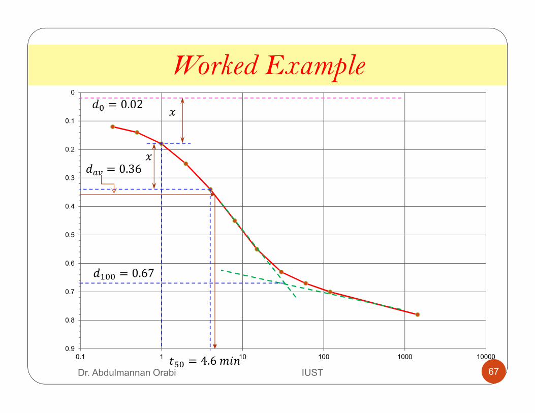
0
0.1
0.2
0.3
0.4
0.5
0.6
0.7
0.8
0.9
0.1 1 10 100 1000 10000
7O = 0.02
7 OO = 0.67
<
<
8[O = 4.6*64
7&9 = 0.36
Worked Example
67Dr. Abdulmannan Orabi IUST
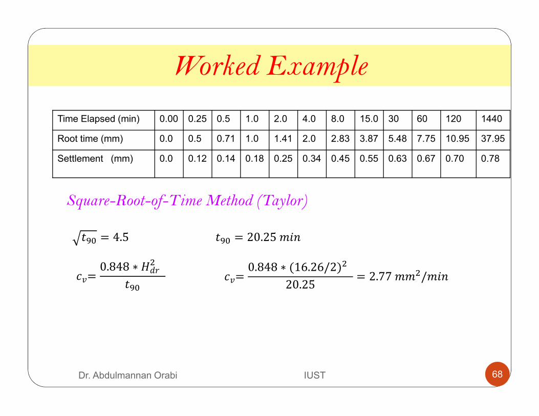
Time Elapsed (min) 0.00 0.25 0.5 1.0 2.0 4.0 8.0 15.0 30 60 120 1440
Root time (mm) 0.0 0.5 0.71 1.0 1.41 2.0 2.83 3.87 5.48 7.75 10.95 37.95
Settlement (mm) 0.0 0.12 0.14 0.18 0.25 0.34 0.45 0.55 0.63 0.67 0.70 0.78
Worked Example
8]O = 20.25*64
-9=0.848 ∗ F73
!
8]O-9=
0.848 ∗ (16.26/2)!
20.25= 2.77**!/*64
Square-Root-of-Time Method (Taylor)
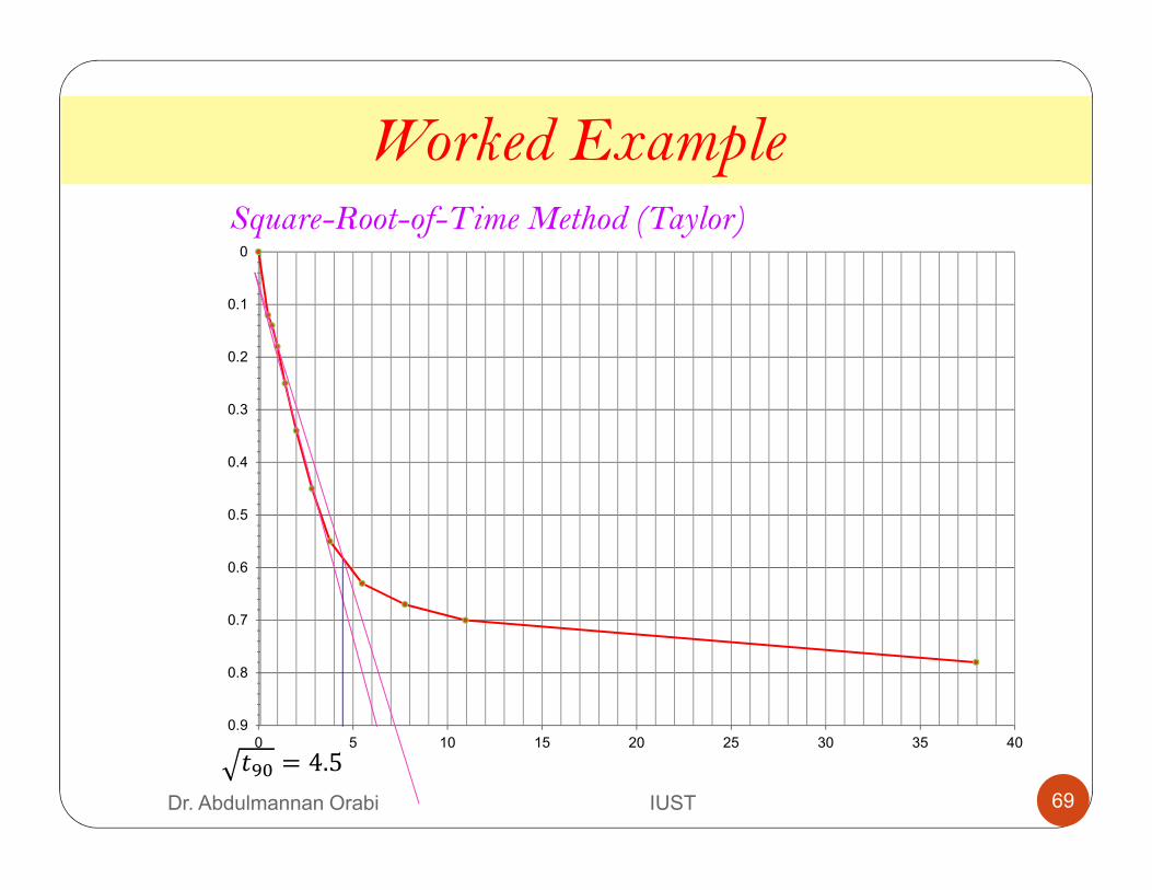
8]O = 4.5
68Dr. Abdulmannan Orabi IUST
0
0.1
0.2
0.3
0.4
0.5
0.6
0.7
0.8
0.9
0 5 10 15 20 25 30 35 40
Square-Root-of-Time Method (Taylor)
8]O = 4.5
Worked Example
69Dr. Abdulmannan Orabi IUST
