lecture 8 : arrangements and duality computational geometry prof. dr. th. ottmann 1 duality and...
Post on 21-Dec-2015
230 views
TRANSCRIPT
1Lecture 8 :Arrangements and Duality
Computational GeometryProf. Dr. Th. Ottmann
Duality and Arrangements
• Duality between lines and points
• Computing the level of points in an arrangement
• Arrangements of line segments
• Half-plane discrepancy
2Lecture 8 :Arrangements and Duality
Computational GeometryProf. Dr. Th. Ottmann
Different duality mappings
A point p = (a,b) and a line l: y= mx + b are uniquely determined by two parameters.
a) Slope mapping: p * = L(p): y = ax + b
b) Polar mapping: p *: ax + by = 1
d) Duality transform:p = (a,b) is mapped to p *: y = ax – bl: y = mx + b is mapped to l* = (m, -b)
c) Parabola mapping: p*: y = ax -b
3Lecture 8 :Arrangements and Duality
Computational GeometryProf. Dr. Th. Ottmann
Duality transform
p = (px, py)
(px, py) → y = pxx – py, y = mx + b → (m, -b)
Characteristics :
1. (p*)* = p = (px, py), (I*)* =l
p*: y = pxx – py
(p*)* = (px, py) = p
(I*)* = I
4Lecture 8 :Arrangements and Duality
Computational GeometryProf. Dr. Th. Ottmann
Characteristics of the duality transform
2) Incidence Preserving :
p = (px, py) lies on l: y = mx+b iff l* lies on p*
p lies on l iff py = mpx + b.
l* lies on p* iff (m, -b) fulfills the equation y = pxx – py iff -b = pxm – py.
5Lecture 8 :Arrangements and Duality
Computational GeometryProf. Dr. Th. Ottmann
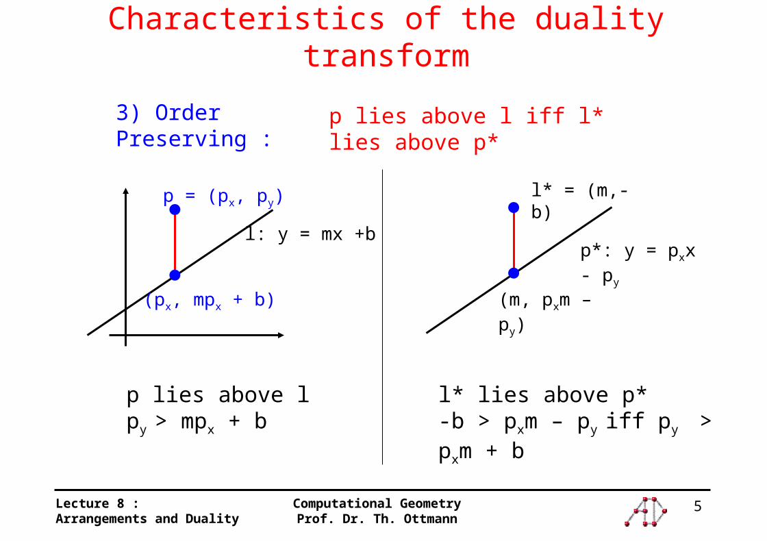
Characteristics of the duality transform
3) Order Preserving : p lies above l iff l* lies above p*
p = (px, py)
(px, mpx + b)
l: y = mx +b
p lies above lpy > mpx + b
l* = (m,-b)
p*: y = pxx - py
(m, pxm – py)
l* lies above p*-b > pxm – py iff py > pxm + b
6Lecture 8 :Arrangements and Duality
Computational GeometryProf. Dr. Th. Ottmann
Summary
Observations:
1. Point p on straight line l iff point l * on straight line p *
2. p above l iff l * above p *
7Lecture 8 :Arrangements and Duality
Computational GeometryProf. Dr. Th. Ottmann
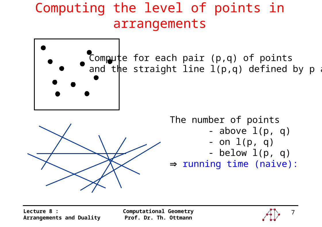
Computing the level of points in arrangements
Compute for each pair (p,q) of pointsand the straight line l(p,q) defined by p and q:
The number of points - above l(p, q) - on l(p, q) - below l(p, q) running time (naive):
8Lecture 8 :Arrangements and Duality
Computational GeometryProf. Dr. Th. Ottmann
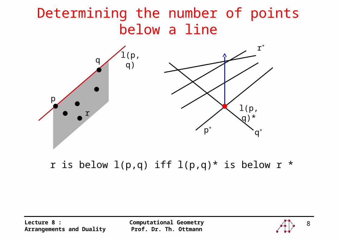
Determining the number of points below a line
r is below l(p,q) iff l(p,q)* is below r *
p
q
r
l(p,q)
p*q*
r*
l(p,q)*
9Lecture 8 :Arrangements and Duality
Computational GeometryProf. Dr. Th. Ottmann
Determining the level of points
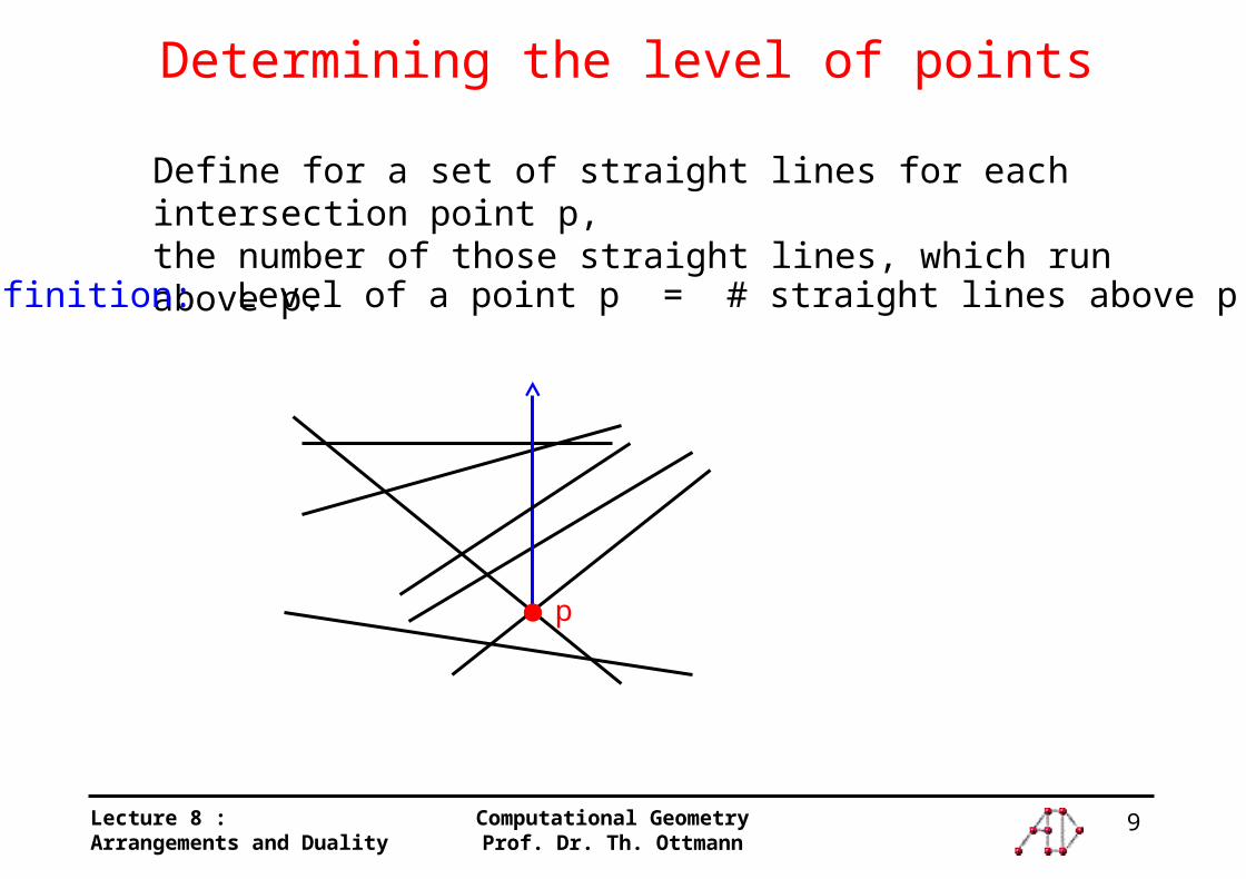
Define for a set of straight lines for each intersection point p,the number of those straight lines, which run above p.
Definition: Level of a point p = # straight lines above p
p
10Lecture 8 :Arrangements and Duality
Computational GeometryProf. Dr. Th. Ottmann
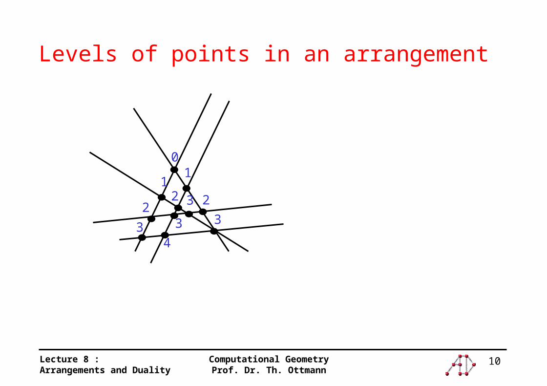
Levels of points in an arrangement
01
1
22 2
3
3
3
4
3

11Lecture 8 :Arrangements and Duality
Computational GeometryProf. Dr. Th. Ottmann
Determining the levels of all Intersections
0 311
pl
Run time : O(n²)
1) Compute the level the leftmost intersection with other lines in time O(n) (comparison with all other straight lines).
2) Walk along the line and update the level at each intersection point
For each straight line:
12Lecture 8 :Arrangements and Duality
Computational GeometryProf. Dr. Th. Ottmann
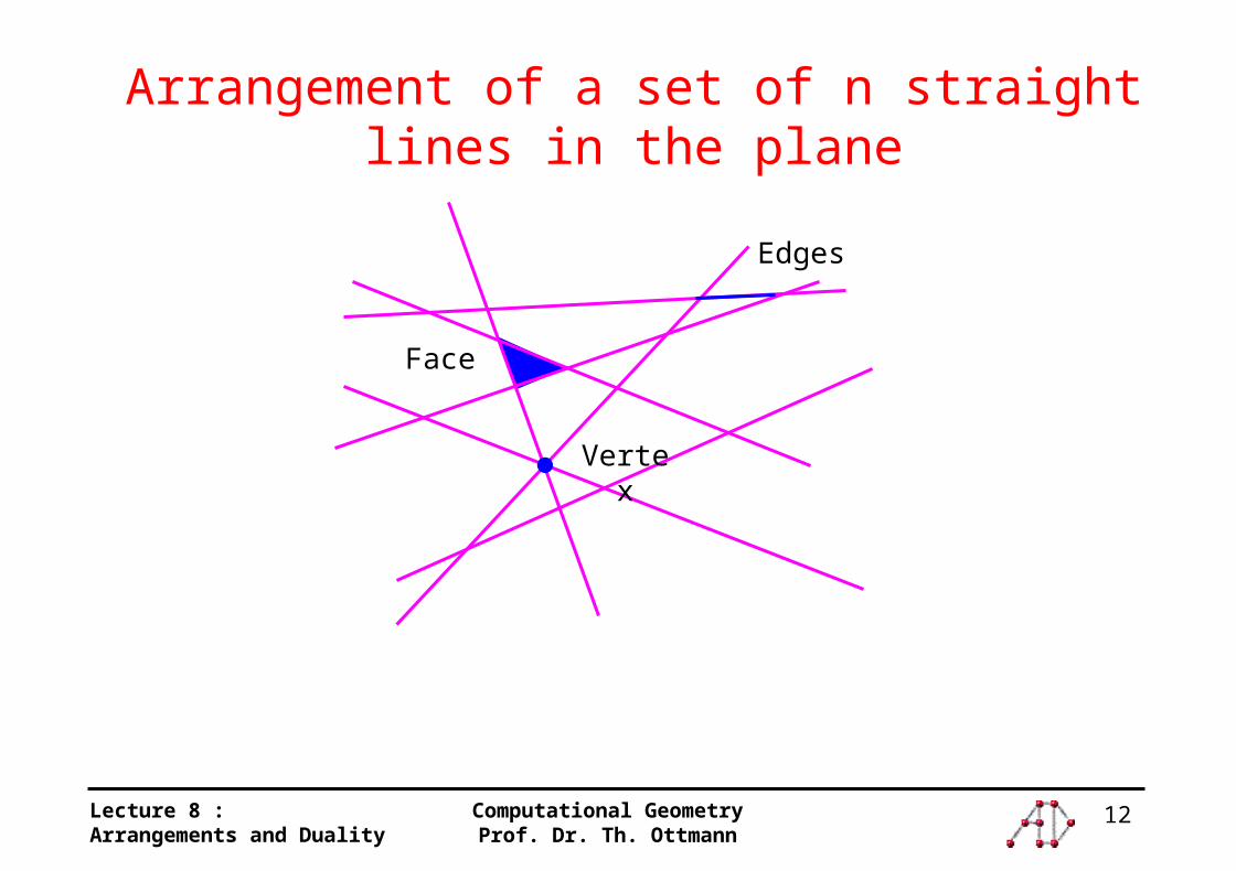
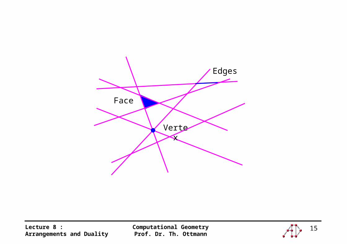
Arrangement of a set of n straight lines in the plane
Edges
Face
Vertex
13Lecture 8 :Arrangements and Duality
Computational GeometryProf. Dr. Th. Ottmann
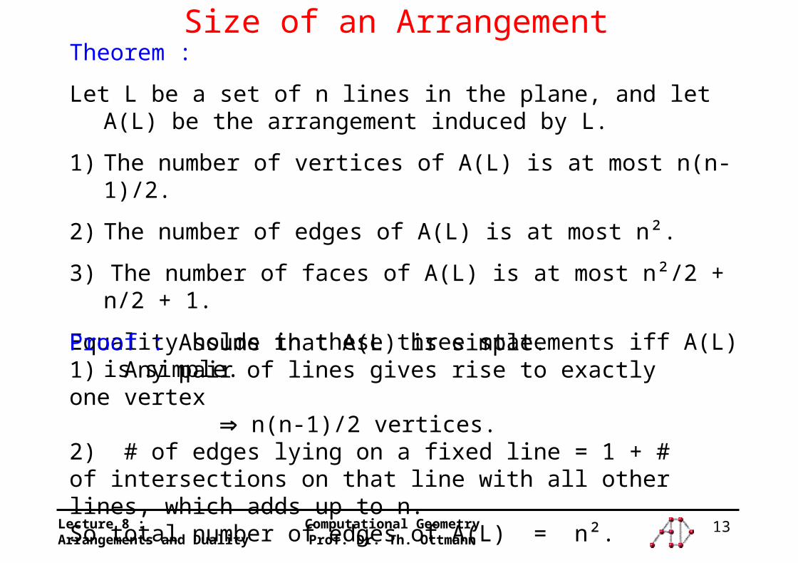
Size of an ArrangementTheorem :
Let L be a set of n lines in the plane, and let A(L) be the arrangement induced by L.
1) The number of vertices of A(L) is at most n(n-1)/2.
2) The number of edges of A(L) is at most n².
3) The number of faces of A(L) is at most n²/2 + n/2 + 1.
Equality holds in these three statements iff A(L) is simple.
Proof : Assume that A(L) is simple. 1) Any pair of lines gives rise to exactly one vertex
n(n-1)/2 vertices.2) # of edges lying on a fixed line = 1 + # of intersections on that line with all other lines, which adds up to n.So total number of edges of A(L) = n².
14Lecture 8 :Arrangements and Duality
Computational GeometryProf. Dr. Th. Ottmann
Proof(Contd...)
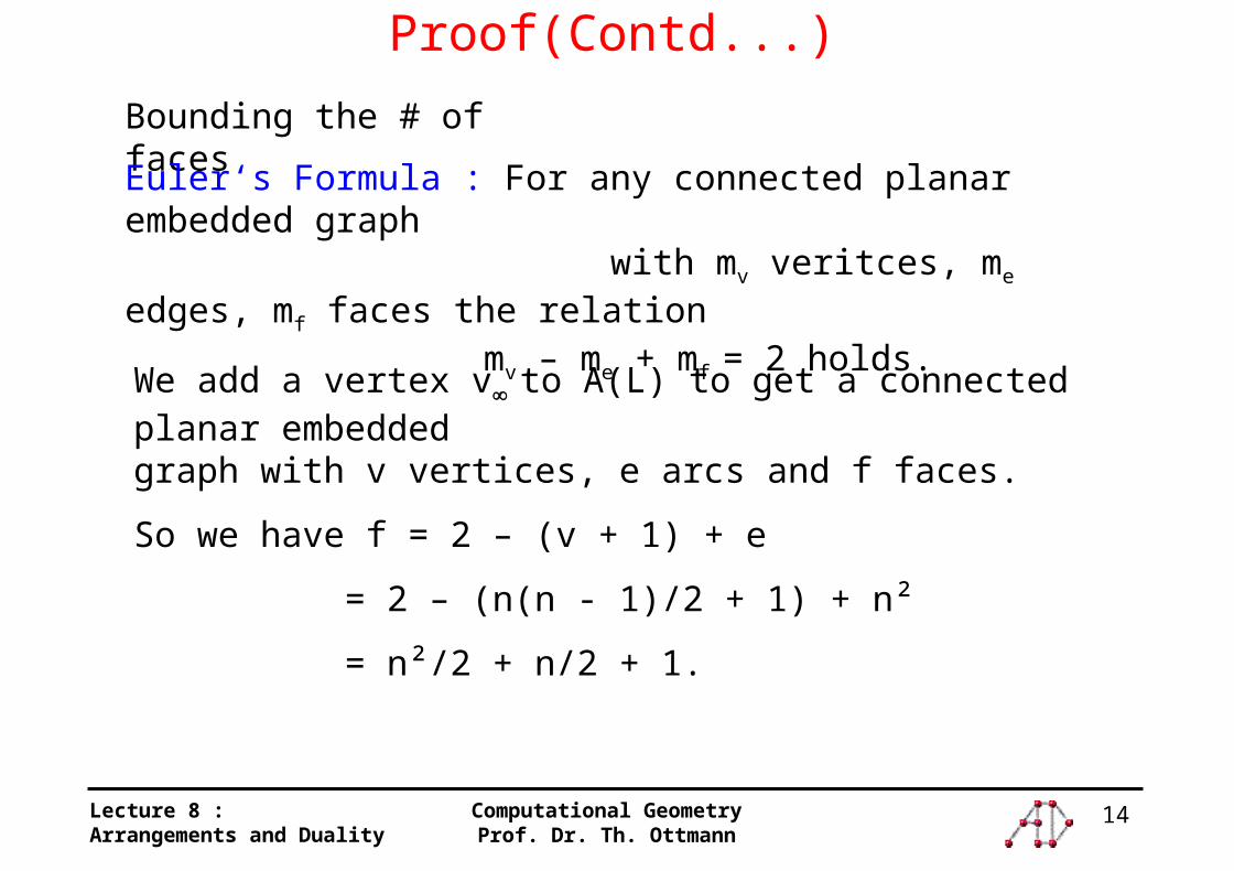
Bounding the # of faces
Euler‘s Formula : For any connected planar embedded graph with mv veritces, me edges, mf faces the relation
mv – me + mf = 2 holds.
We add a vertex v to A(L) to get a connected planar embeddedgraph with v vertices, e arcs and f faces.
So we have f = 2 – (v + 1) + e
= 2 – (n(n - 1)/2 + 1) + n²
= n²/2 + n/2 + 1.
15Lecture 8 :Arrangements and Duality
Computational GeometryProf. Dr. Th. Ottmann
Edges
Face
Vertex
16Lecture 8 :Arrangements and Duality
Computational GeometryProf. Dr. Th. Ottmann
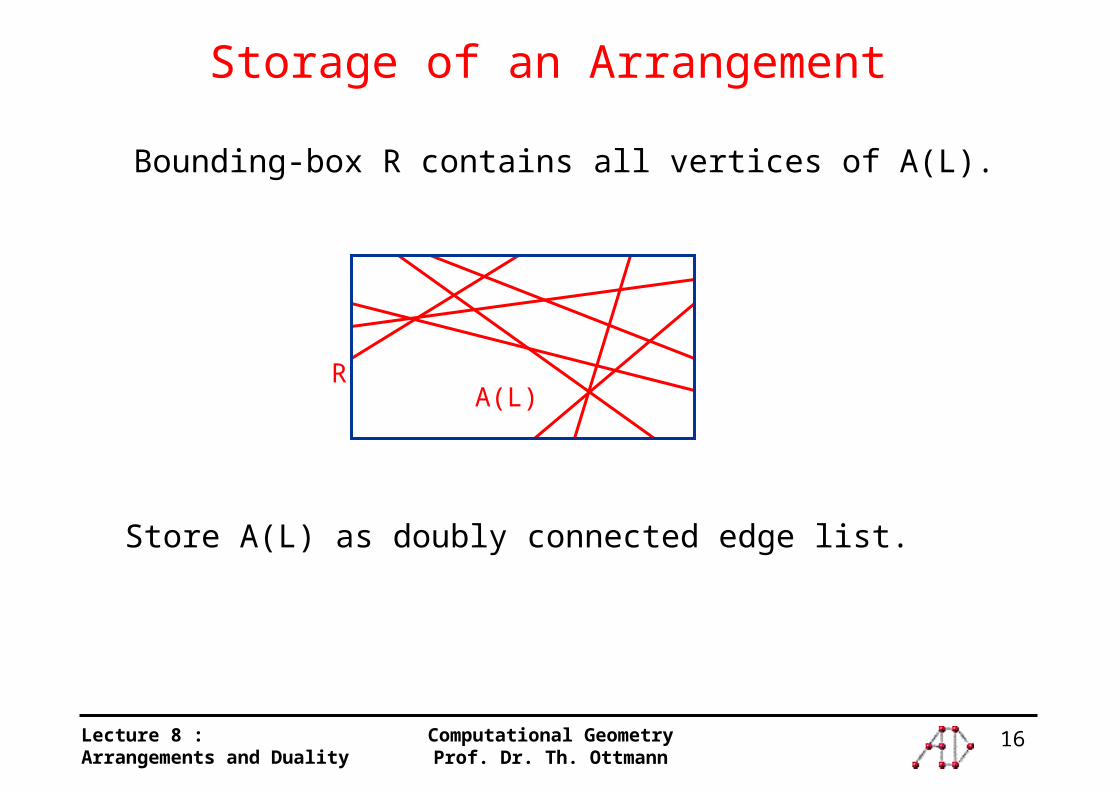
Storage of an Arrangement
A(L)R
Bounding-box R contains all vertices of A(L).
Store A(L) as doubly connected edge list.
17Lecture 8 :Arrangements and Duality
Computational GeometryProf. Dr. Th. Ottmann
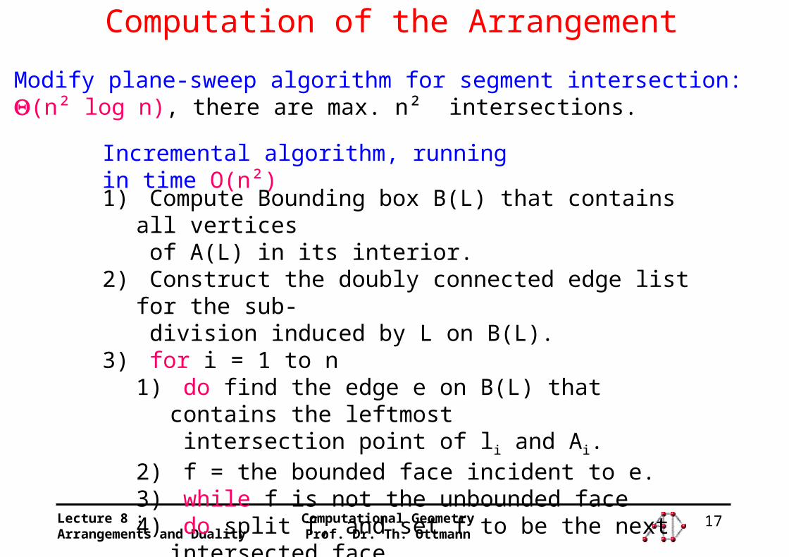
Computation of the Arrangement
Modify plane-sweep algorithm for segment intersection:(n² log n), there are max. n² intersections.
Incremental algorithm, running in time O(n²)
1) Compute Bounding box B(L) that contains all vertices of A(L) in its interior.
2) Construct the doubly connected edge list for the sub- division induced by L on B(L).
3) for i = 1 to n1) do find the edge e on B(L) that contains the leftmost
intersection point of li and Ai.2) f = the bounded face incident to e.3) while f is not the unbounded face 4) do split f, and set f to be the next intersected face.
18Lecture 8 :Arrangements and Duality
Computational GeometryProf. Dr. Th. Ottmann
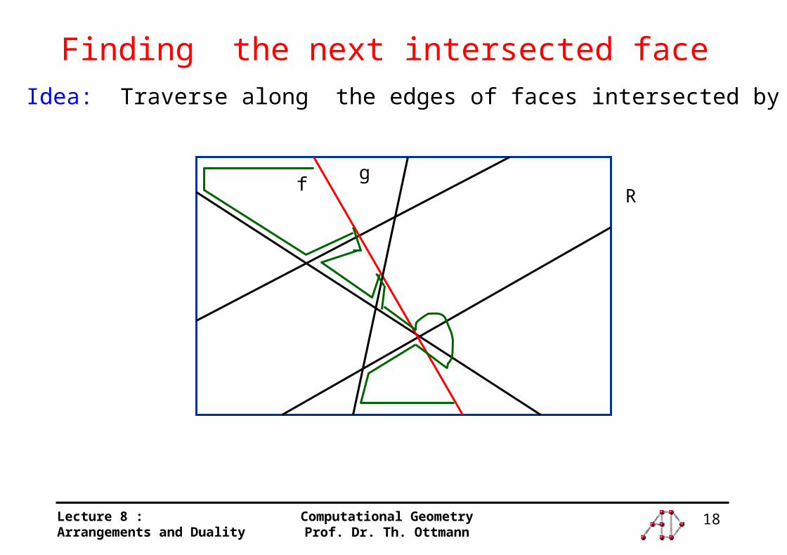
Finding the next intersected faceIdea: Traverse along the edges of faces intersected by g
fg
R
19Lecture 8 :Arrangements and Duality
Computational GeometryProf. Dr. Th. Ottmann
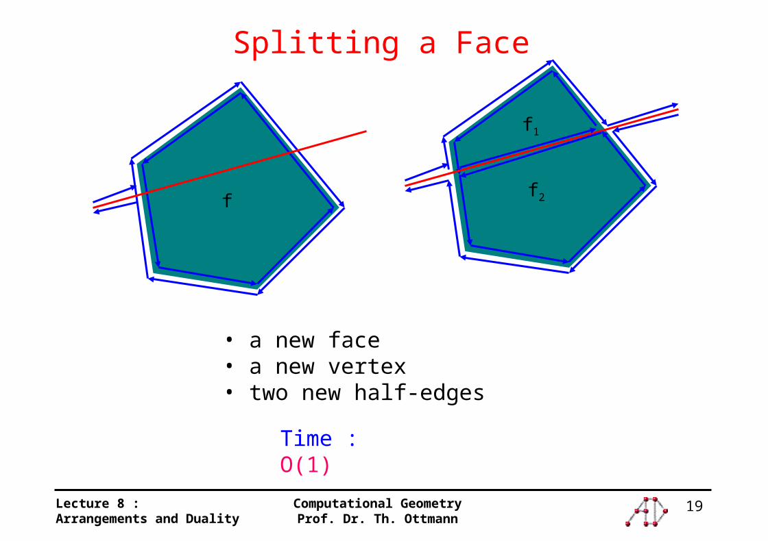
Splitting a Face
f
f1
f2
• a new face• a new vertex• two new half-edges
Time : O(1)
20Lecture 8 :Arrangements and Duality
Computational GeometryProf. Dr. Th. Ottmann
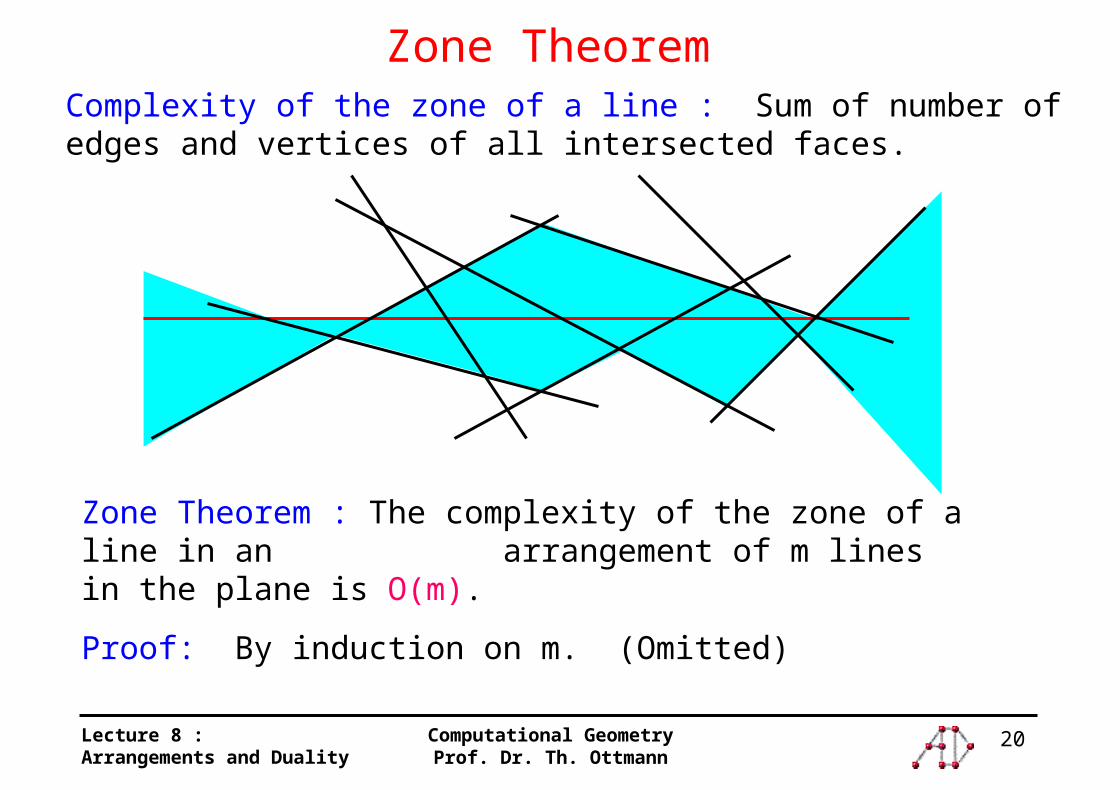
Zone TheoremComplexity of the zone of a line : Sum of number of edges and vertices of all intersected faces.
Zone Theorem : The complexity of the zone of a line in an arrangement of m lines in the plane is O(m).
Proof: By induction on m. (Omitted)
21Lecture 8 :Arrangements and Duality
Computational GeometryProf. Dr. Th. Ottmann
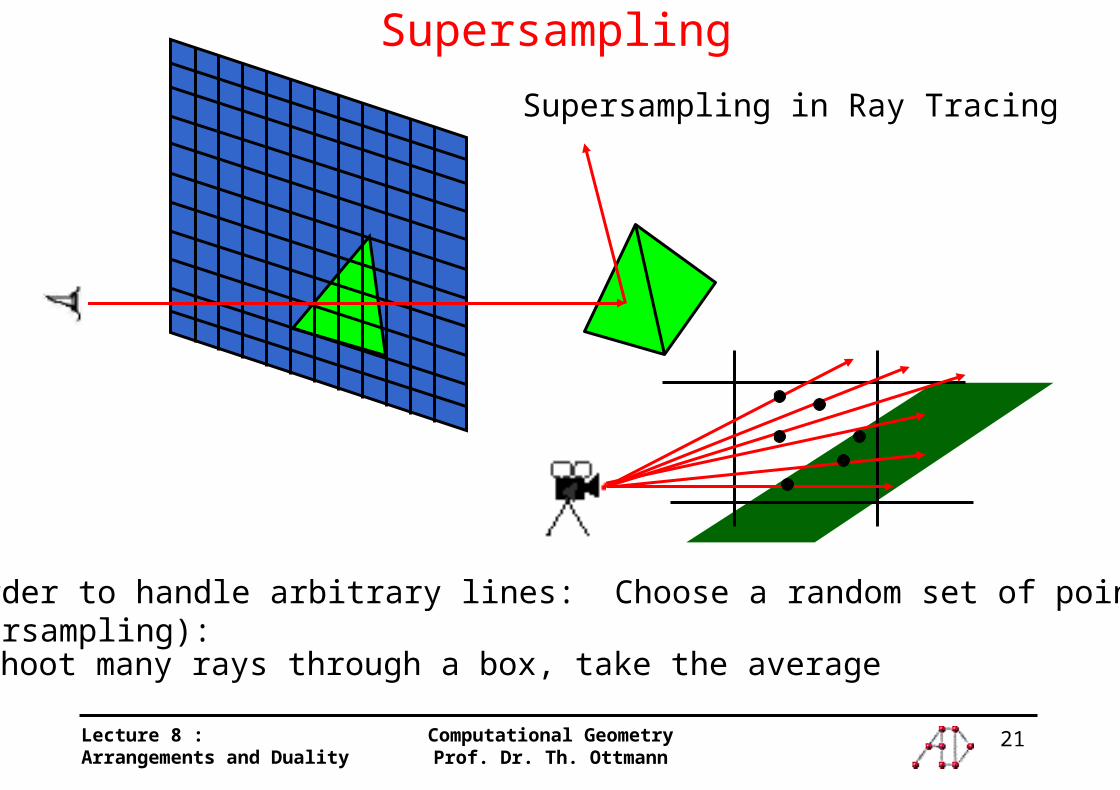
Supersampling
Supersampling in Ray Tracing
In order to handle arbitrary lines: Choose a random set of points(Supersampling):Shoot many rays through a box, take the average
22Lecture 8 :Arrangements and Duality
Computational GeometryProf. Dr. Th. Ottmann
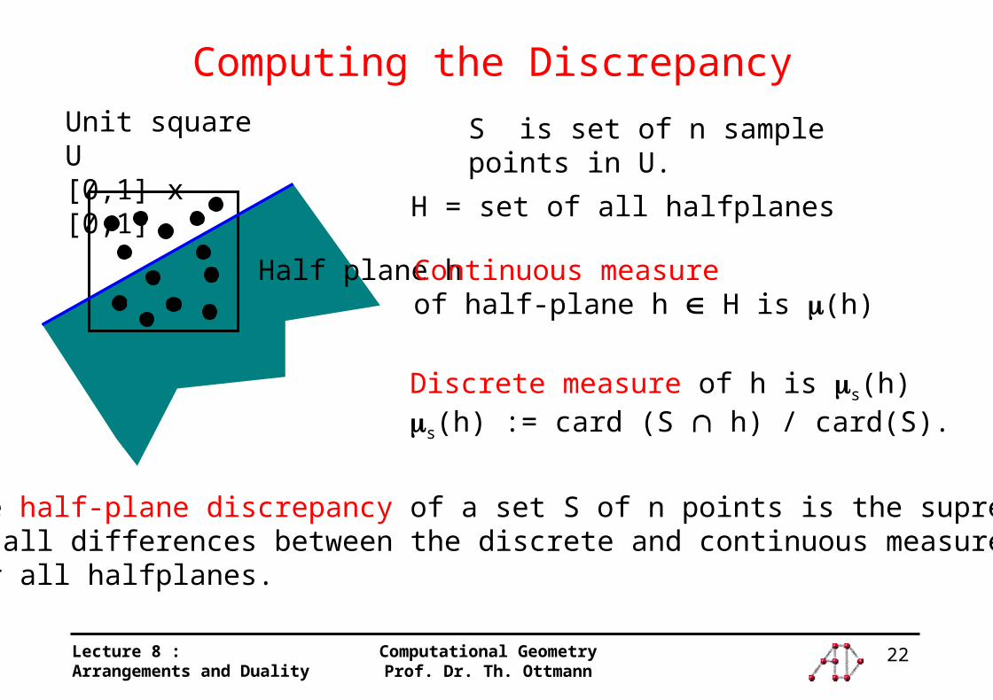
Computing the DiscrepancyUnit square U[0,1] x [0,1]
Half plane h
S is set of n sample points in U.
Discrete measure of h is s(h) s(h) := card (S h) / card(S).
H = set of all halfplanes
Continuous measure of half-plane h H is (h)
The half-plane discrepancy of a set S of n points is the supremumof all differences between the discrete and continuous measuresfor all halfplanes.
23Lecture 8 :Arrangements and Duality
Computational GeometryProf. Dr. Th. Ottmann
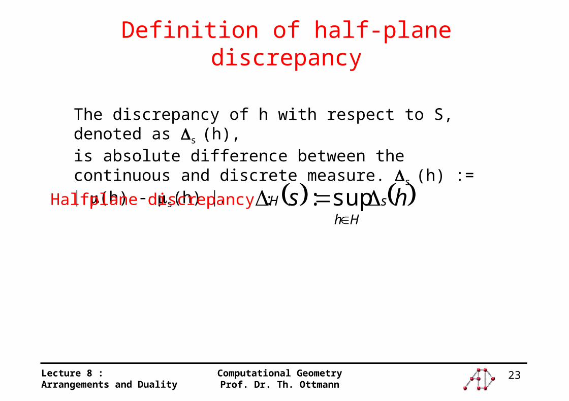
The discrepancy of h with respect to S, denoted as s (h),is absolute difference between the continuous and discrete measure. s (h) := (h) - s(h) .
Halfplane discrepancy : hs sHh
H sup:
Definition of half-plane discrepancy

24Lecture 8 :Arrangements and Duality
Computational GeometryProf. Dr. Th. Ottmann
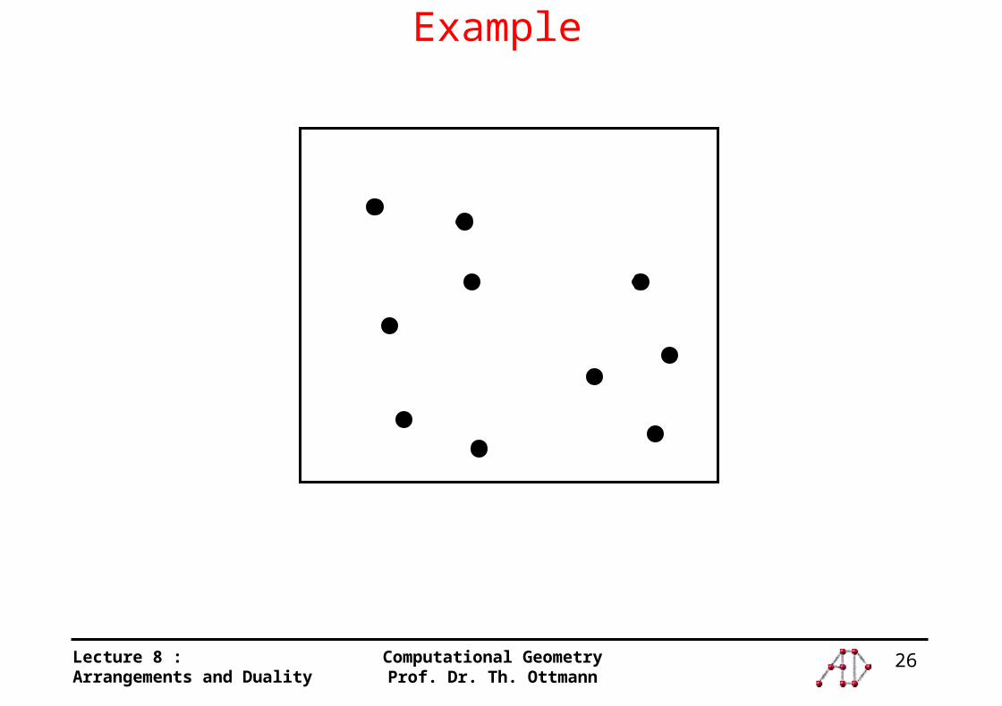
Example

25Lecture 8 :Arrangements and Duality
Computational GeometryProf. Dr. Th. Ottmann
Computing the Discrepancy(contd...)
Lemma : Let S be a set of n points in the unit square U.
A half-plane h that achieves the maximum discrepancy with respect to S is of one of the following types :
1. h contains one point p S on its boundary. 2. h contains 2 or more points of S on its boundary.
The number of type(1) candidates is O(n), and they can be found in O(n) time.
26Lecture 8 :Arrangements and Duality
Computational GeometryProf. Dr. Th. Ottmann
Example
27Lecture 8 :Arrangements and Duality
Computational GeometryProf. Dr. Th. Ottmann
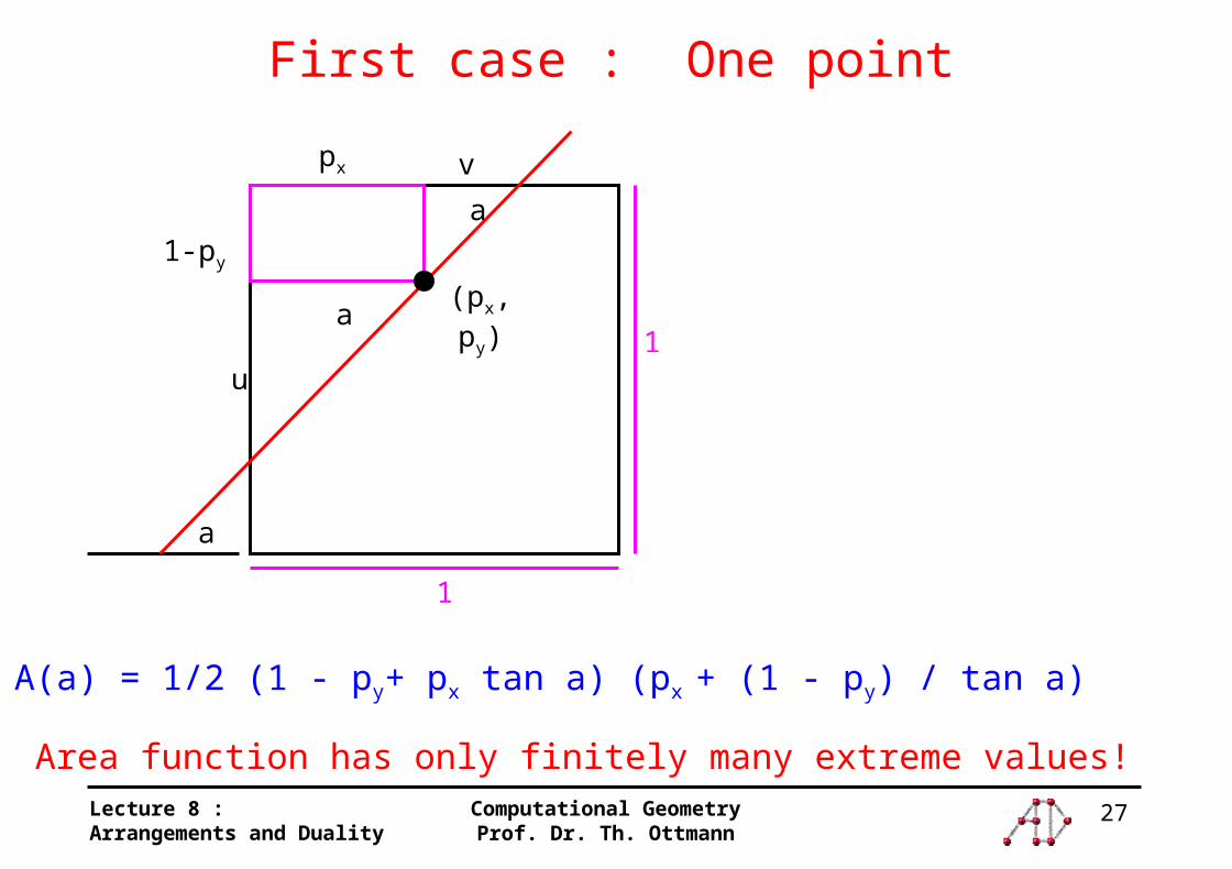
First case : One point
px
1-py
(px, py)
u
v
a
a
a
1
1
A(a) = 1/2 (1 - py+ px tan a) (px + (1 - py) / tan a)
Area function has only finitely many extreme values!
28Lecture 8 :Arrangements and Duality
Computational GeometryProf. Dr. Th. Ottmann
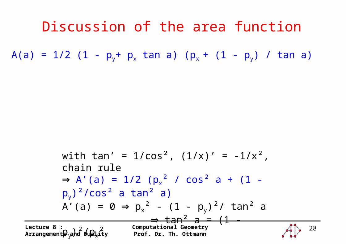
A(a) = 1/2 (1 - py+ px tan a) (px + (1 - py) / tan a)
with tan’ = 1/cos², (1/x)’ = -1/x², chain rule A’(a) = 1/2 (px² / cos² a + (1 - py)²/cos² a tan² a)A’(a) = 0 px² - (1 - py)²/ tan² a tan² a = (1 - py)²/px²
Discussion of the area function