CS231M · Mobile Computer Vision

Lecture 7

Optical flow and tracking- Introduction

- Optical flow & KLT tracker

- Motion segmentation

Forsyth, Ponce “Computer vision: a modern approach”:- Chapter 10, Sec 10.6- Chapter 11, Sec 11.1

Szeliski, “Computer Vision: algorithms and applications"- Chapter 8, Sec. 8.5

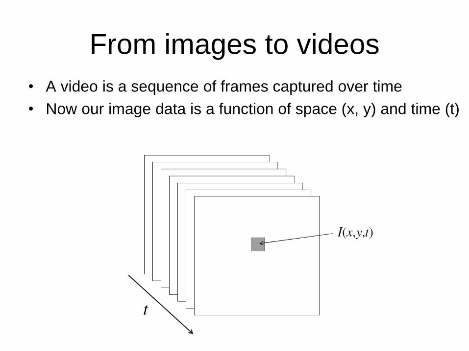
From images to videos

• A video is a sequence of frames captured over time

• Now our image data is a function of space (x, y) and time (t)

Uses of motion

• Improving video quality

– Motion stabilization

– Super resolution

• Segmenting objects based on motion cues

• Tracking objects

• Recognizing events and activities

4

Example: A set of low

quality images

• Irani, M.; Peleg, S. (June 1990). "Super Resolution From Image Sequences". International Conference on Pattern Recognition

• Fast and Robust Multiframe Super Resolution, Sina Farsiu, M. Dirk Robinson, Michael Elad, and Peyman Milanfar, EEE TRANSACTIONS ON

IMAGE PROCESSING, VOL. 13, NO. 10, OCTOBER 2004

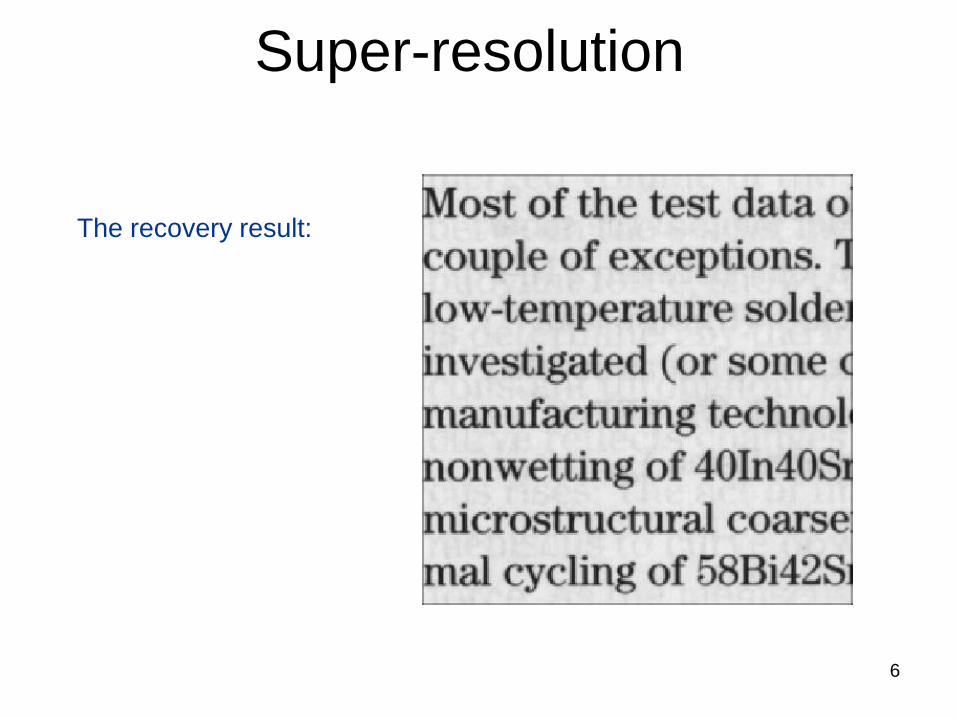
Super-resolution

5

Each of these images

looks like this:

Super-resolution

6

The recovery result:

Super-resolution

Visual SLAM

Courtesy of Jean-Yves Bouguet – Vision Lab, California Institute of Technology

Segmenting objects based on

motion cues

• Background subtraction

– A static camera is observing a scene

– Goal: separate the static background from the moving foreground

https://www.youtube.com/watch?v=YAszeOaInUMSuha Kwak, Taegyu Lim, Woonhyun Nam, Bohyung Han, Joon Hee Han: Generalized background subtraction based on hybrid inference by belief propagation and Bayesian filtering. ICCV 2011

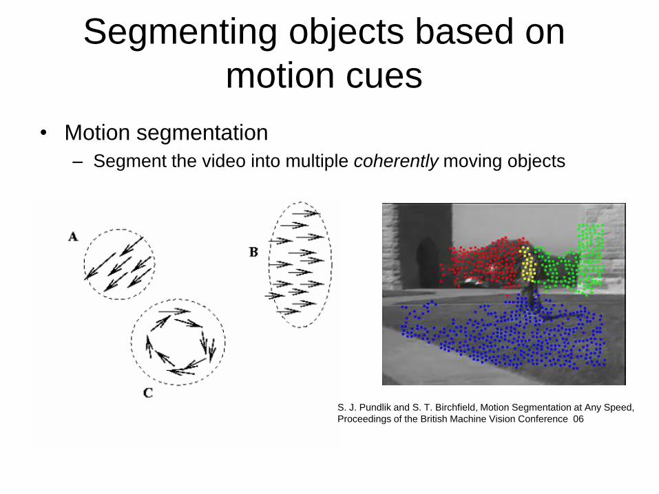
• Motion segmentation

– Segment the video into multiple coherently moving objects

S. J. Pundlik and S. T. Birchfield, Motion Segmentation at Any Speed,

Proceedings of the British Machine Vision Conference 06

Segmenting objects based on

motion cues

Tracking objects

• Facing tracking on openCV

http://www.youtube.com/watch?v=HTk_UwAYzVk

OpenCV's face tracker uses an algorithm called Camshift (based on the meanshift algorithm)

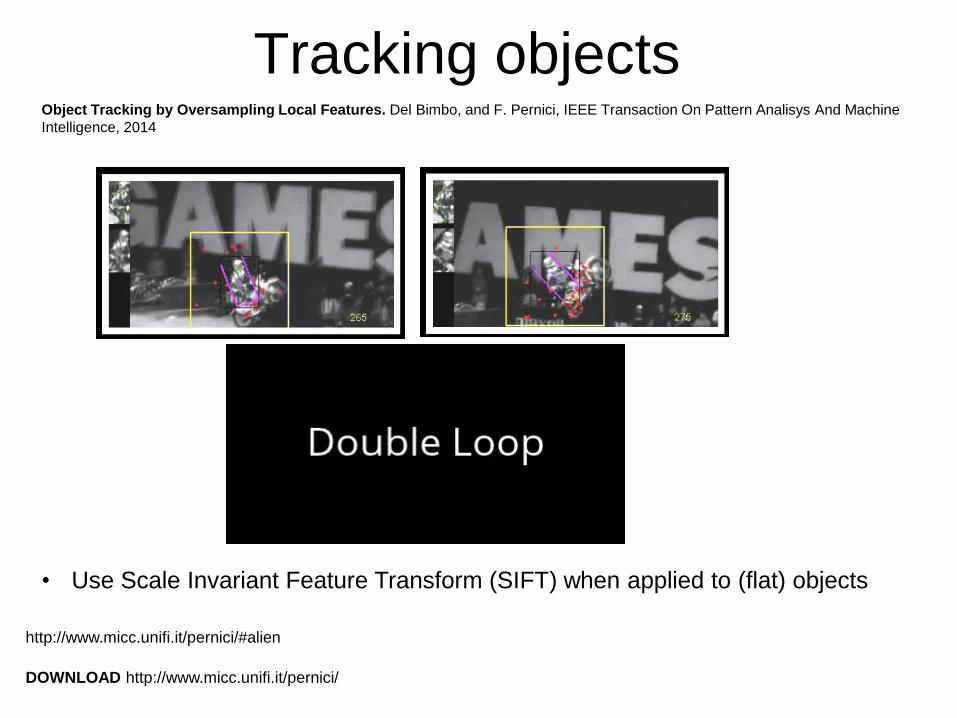
Object Tracking by Oversampling Local Features. Del Bimbo, and F. Pernici, IEEE Transaction On Pattern Analisys And Machine

Intelligence, 2014

DOWNLOAD http://www.micc.unifi.it/pernici/

• Use Scale Invariant Feature Transform (SIFT) when applied to (flat) objects

http://www.micc.unifi.it/pernici/#alien

Tracking objects

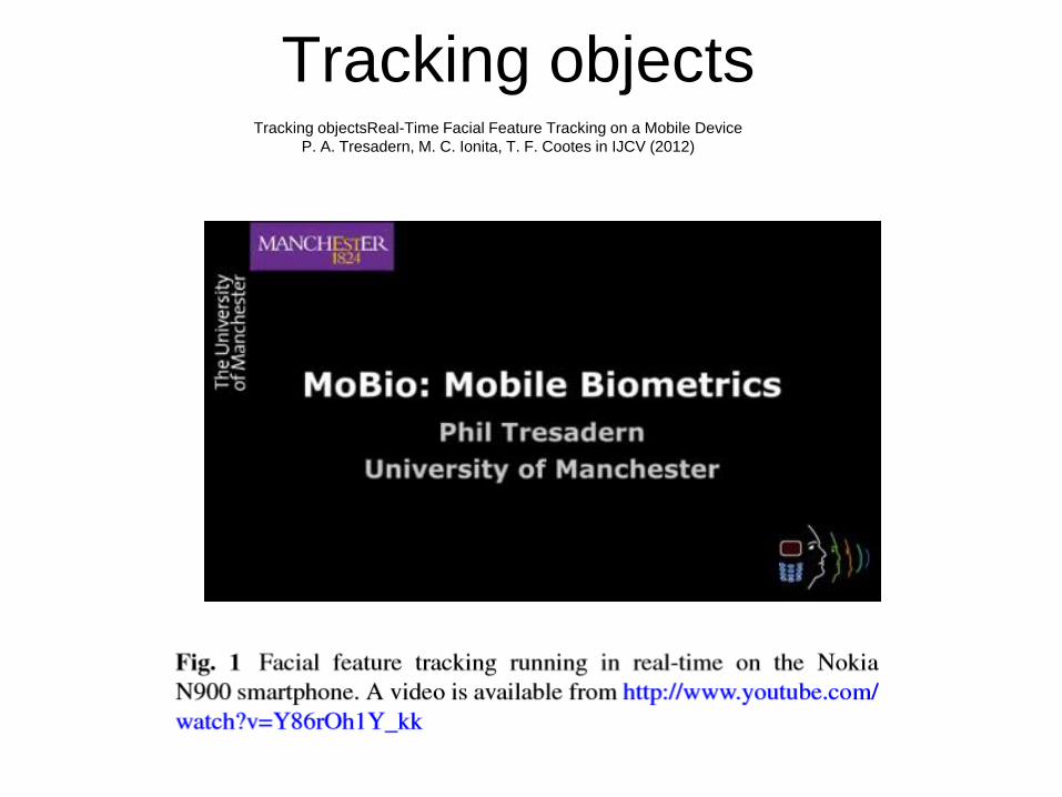
Tracking objectsTracking objectsReal-Time Facial Feature Tracking on a Mobile Device

P. A. Tresadern, M. C. Ionita, T. F. Cootes in IJCV (2012)

Joint tracking and 3D localization

W. Choi & K. Shahid & S. Savarese WMC 2009

W. Choi & S. Savarese , ECCV, 2010

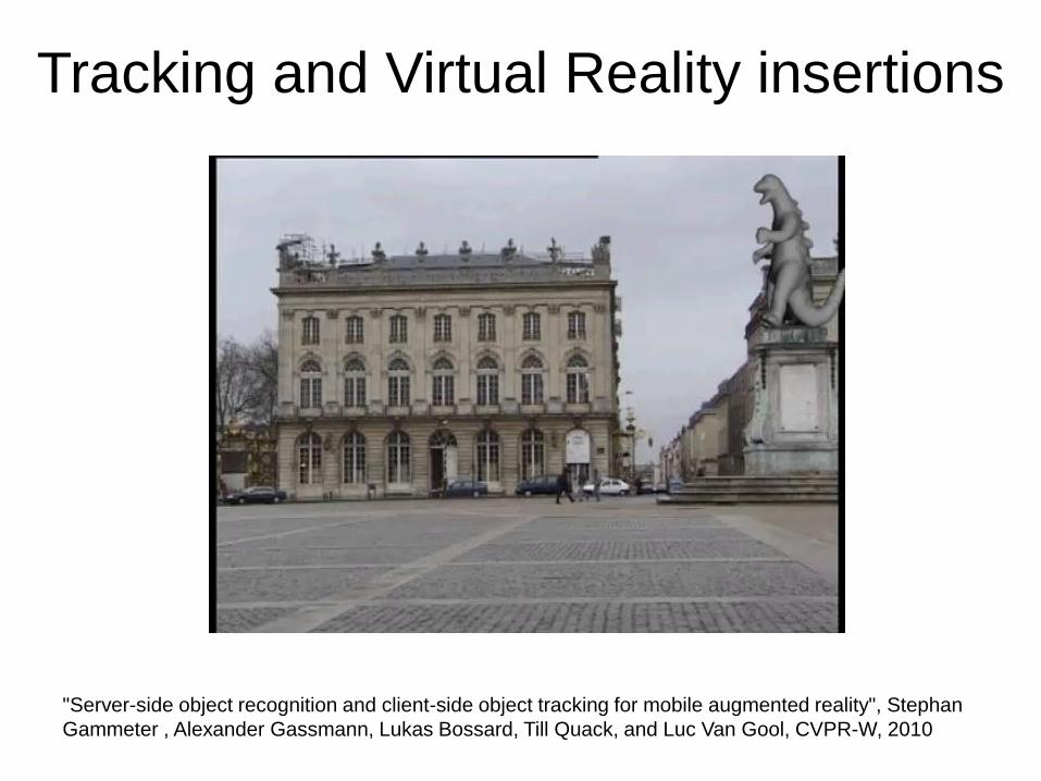
Tracking and Virtual Reality insertions

"Server-side object recognition and client-side object tracking for mobile augmented reality", Stephan

Gammeter , Alexander Gassmann, Lukas Bossard, Till Quack, and Luc Van Gool, CVPR-W, 2010

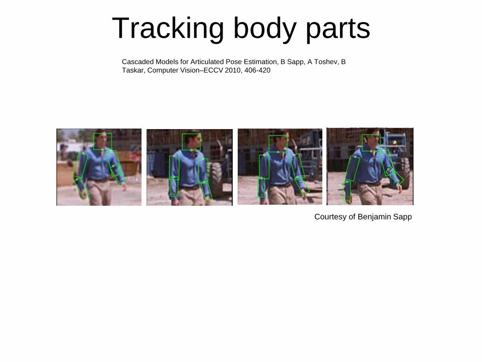
Tracking body parts

Courtesy of Benjamin Sapp

Cascaded Models for Articulated Pose Estimation, B Sapp, A Toshev, B

Taskar, Computer Vision–ECCV 2010, 406-420

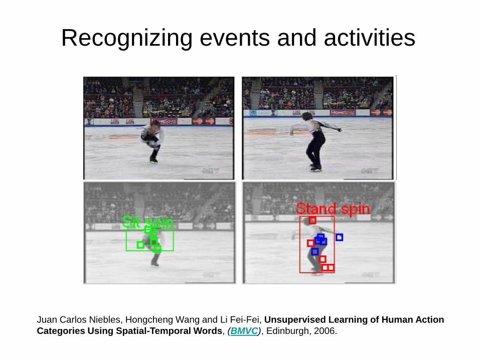
Juan Carlos Niebles, Hongcheng Wang and Li Fei-Fei, Unsupervised Learning of Human Action

Categories Using Spatial-Temporal Words, (BMVC), Edinburgh, 2006.

Recognizing events and activities

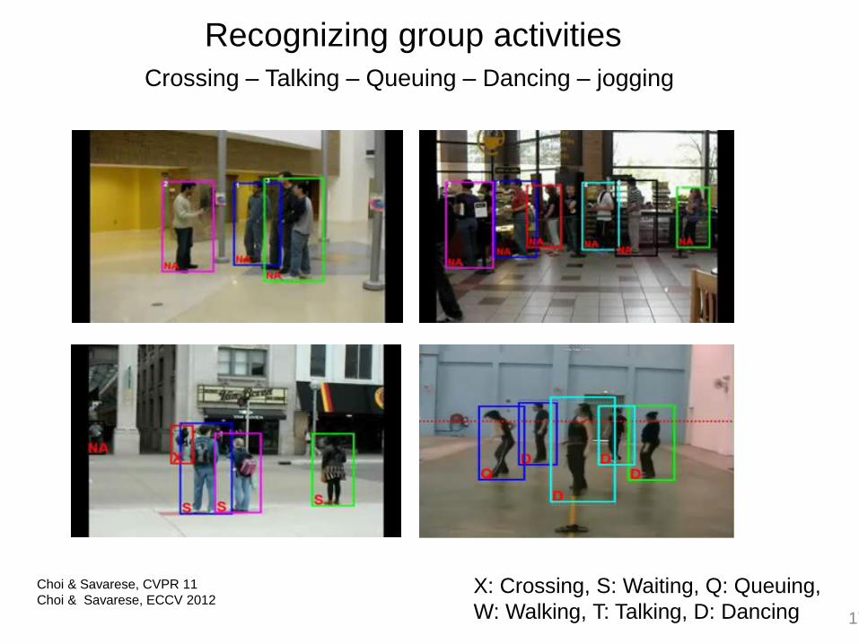
X: Crossing, S: Waiting, Q: Queuing,

W: Walking, T: Talking, D: Dancing 17

Choi & Savarese, CVPR 11

Choi & Savarese, ECCV 2012

Crossing – Talking – Queuing – Dancing – jogging

Recognizing group activities

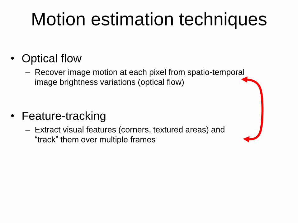
Motion estimation techniques

• Optical flow– Recover image motion at each pixel from spatio-temporal

image brightness variations (optical flow)

• Feature-tracking– Extract visual features (corners, textured areas) and

“track” them over multiple frames

Optical flowVector field function of the spatio-temporal image brightness variations

Picture courtesy of Selim Temizer - Learning and Intelligent Systems (LIS) Group, MIT

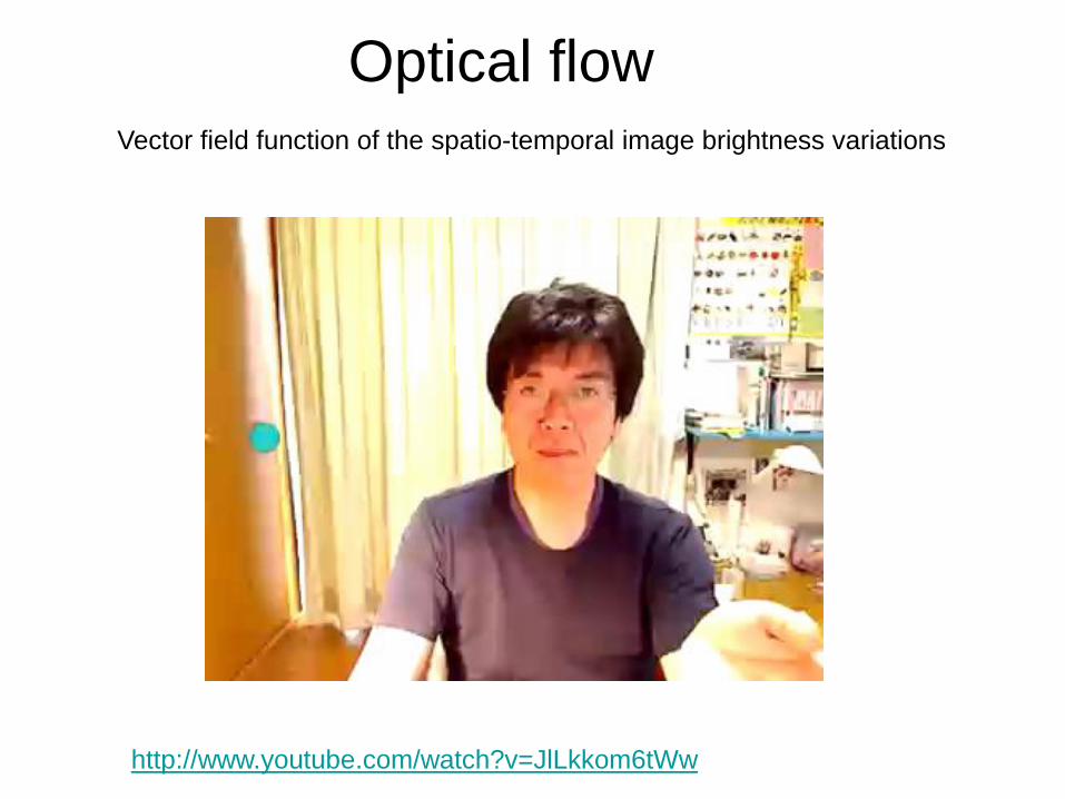
Optical flowVector field function of the spatio-temporal image brightness variations

http://www.youtube.com/watch?v=JlLkkom6tWw

Optical flow

Definition: optical flow is the apparent motion of

brightness patterns in the image

GOAL: Recover image motion at each pixel by

optical flow

Note: apparent motion can be caused by lighting changes without

any actual motion

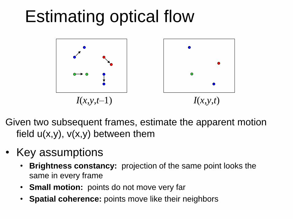
Estimating optical flow

Given two subsequent frames, estimate the apparent motion

field u(x,y), v(x,y) between them

• Key assumptions• Brightness constancy: projection of the same point looks the

same in every frame

• Small motion: points do not move very far

• Spatial coherence: points move like their neighbors

I(x,y,t–1) I(x,y,t)

tyx IyxvIyxuItyxItuyuxI ),(),()1,,(),,(

Brightness Constancy Equation:

),()1,,( ),,(),( tyxyx vyuxItyxI

Linearizing the right side using Taylor expansion:

The brightness constancy constraint

I(x,y,t–1) I(x,y,t)

0 tyx IvIuIHence, 0IvuI t

T

tyx IyxvIyxuItyxItuyuxI ),(),()1,,(),,(

u

v

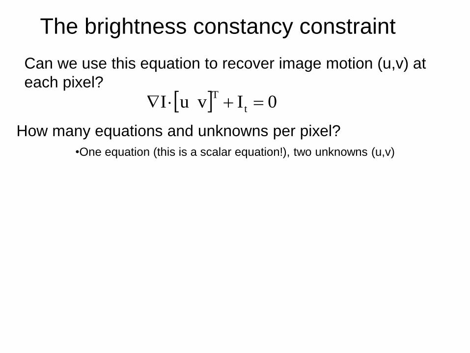
The brightness constancy constraint

How many equations and unknowns per pixel?

•One equation (this is a scalar equation!), two unknowns (u,v)

0IvuI t

T

Can we use this equation to recover image motion (u,v) at

each pixel?

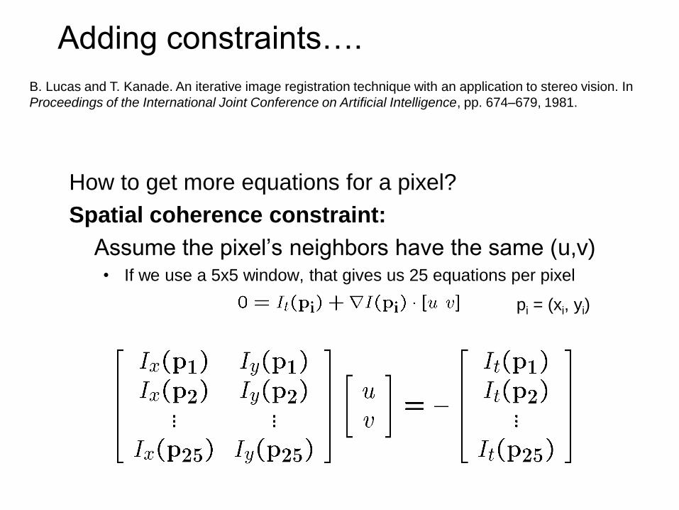
Adding constraints….

How to get more equations for a pixel?

Spatial coherence constraint:

Assume the pixel’s neighbors have the same (u,v)• If we use a 5x5 window, that gives us 25 equations per pixel

B. Lucas and T. Kanade. An iterative image registration technique with an application to stereo vision. In

Proceedings of the International Joint Conference on Artificial Intelligence, pp. 674–679, 1981.

pi = (xi, yi)

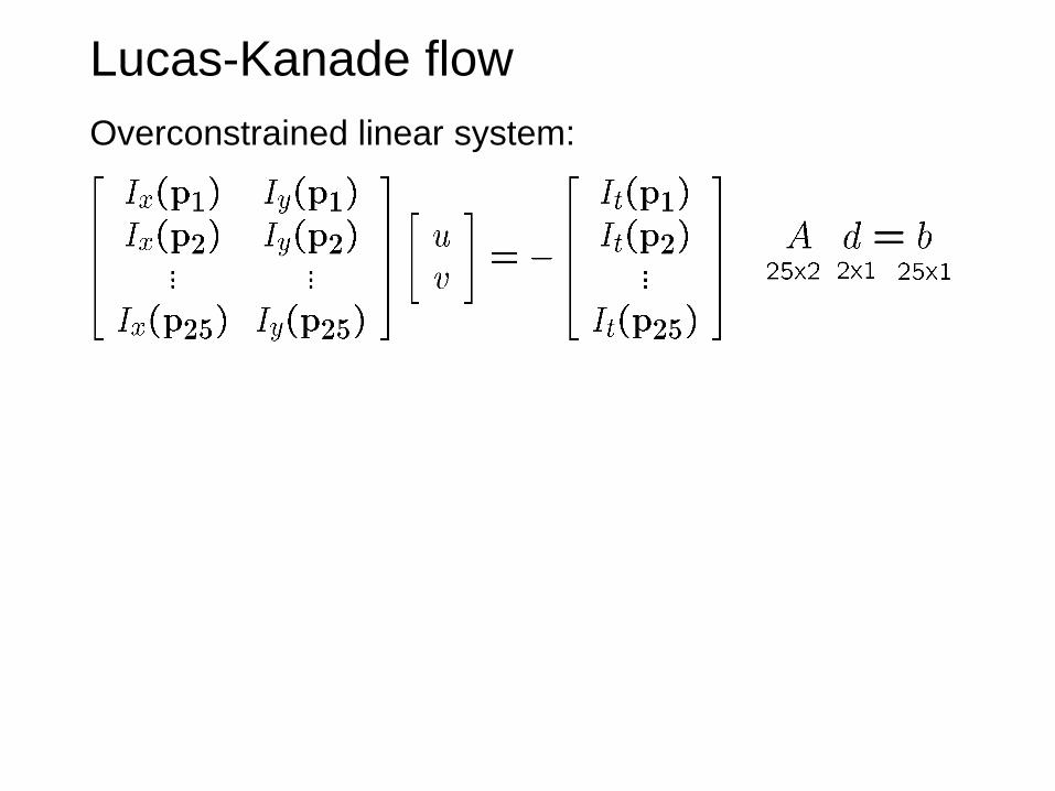
Overconstrained linear system:

Lucas-Kanade flow

Lucas-Kanade flow

Overconstrained linear system

The summations are over all pixels in the K x K window

Least squares solution for d given by

Conditions for solvability

• Optimal (u, v) satisfies Lucas-Kanade equation

Does this remind anything to you?

When is this solvable?• ATA should be invertible

• Eigenvalues 1 and 2 of ATA should not be too small

• ATA should be well-conditioned

– 1/ 2 should not be too large ( 1 = larger eigenvalue)

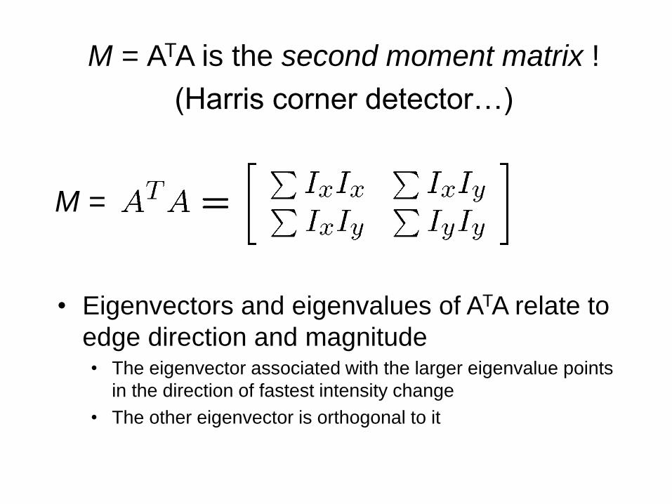
• Eigenvectors and eigenvalues of ATA relate to

edge direction and magnitude • The eigenvector associated with the larger eigenvalue points

in the direction of fastest intensity change

• The other eigenvector is orthogonal to it

M = ATA is the second moment matrix !

(Harris corner detector…)

M =

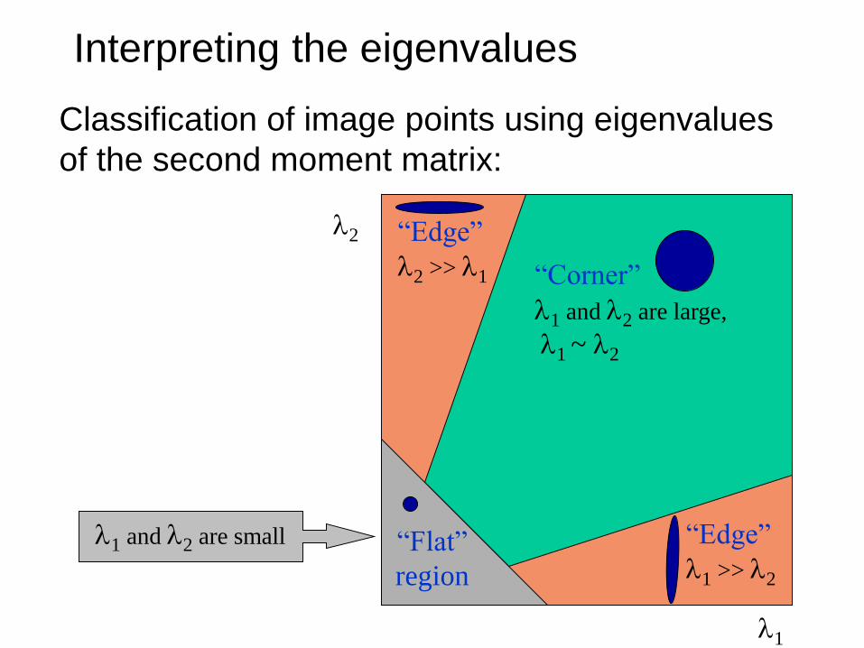
Interpreting the eigenvalues

1

2

“Corner”

1 and 2 are large,

1 ~ 2

1 and 2 are small “Edge”

1 >> 2

“Edge”

2 >> 1

“Flat”

region

Classification of image points using eigenvalues

of the second moment matrix:

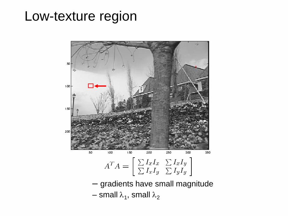
Low-texture region

– gradients have small magnitude

– small 1, small 2

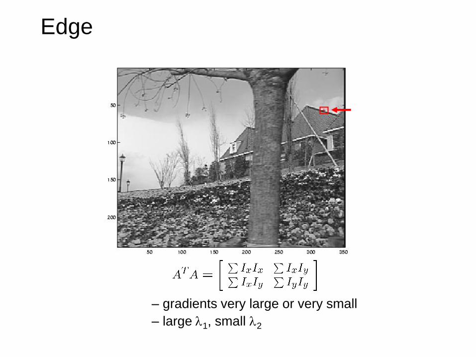
Edge

– gradients very large or very small

– large 1, small 2

High-texture region

– gradients are different, large magnitudes

– large 1, large 2

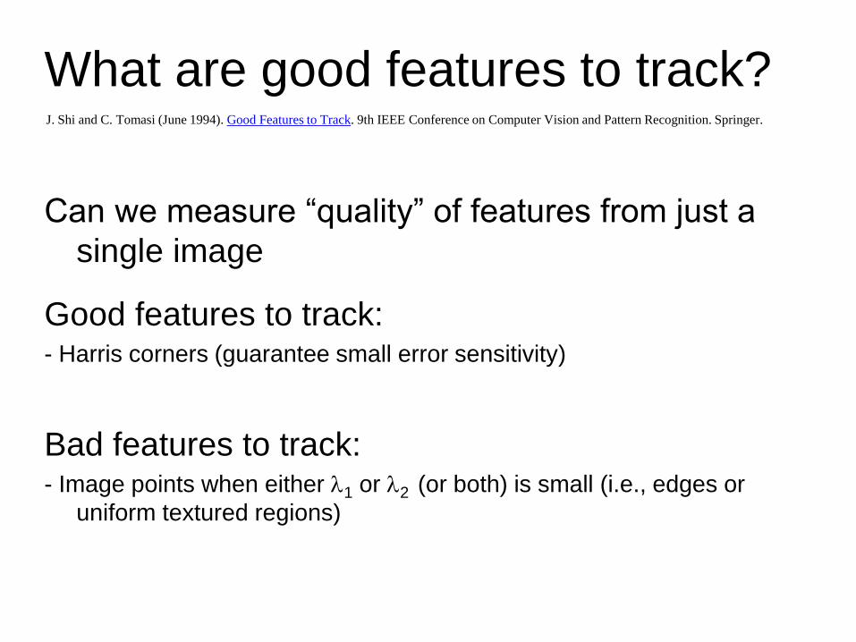
What are good features to track?

Can we measure “quality” of features from just a

single image

Good features to track:- Harris corners (guarantee small error sensitivity)

Bad features to track:- Image points when either 1 or 2 (or both) is small (i.e., edges or

uniform textured regions)

J. Shi and C. Tomasi (June 1994). Good Features to Track. 9th IEEE Conference on Computer Vision and Pattern Recognition. Springer.

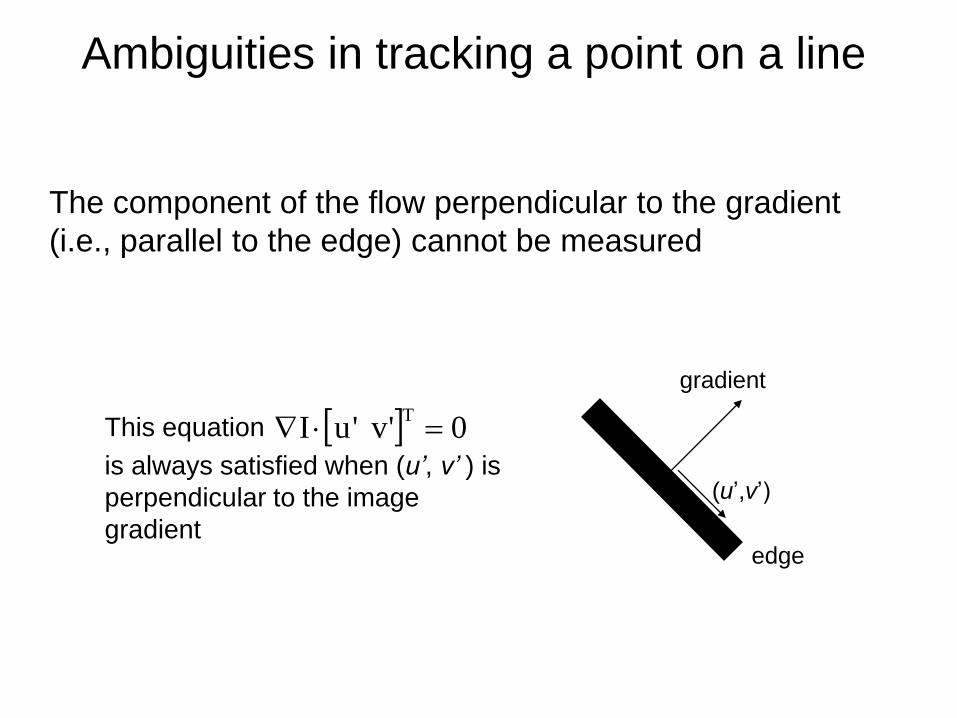
(u’,v’)

Ambiguities in tracking a point on a line

The component of the flow perpendicular to the gradient

(i.e., parallel to the edge) cannot be measured

edge

gradient

This equation

is always satisfied when (u’, v’ ) is

perpendicular to the image

gradient

0'v'uIT

The barber pole illusion

http://en.wikipedia.org/wiki/Barberpole_illusion

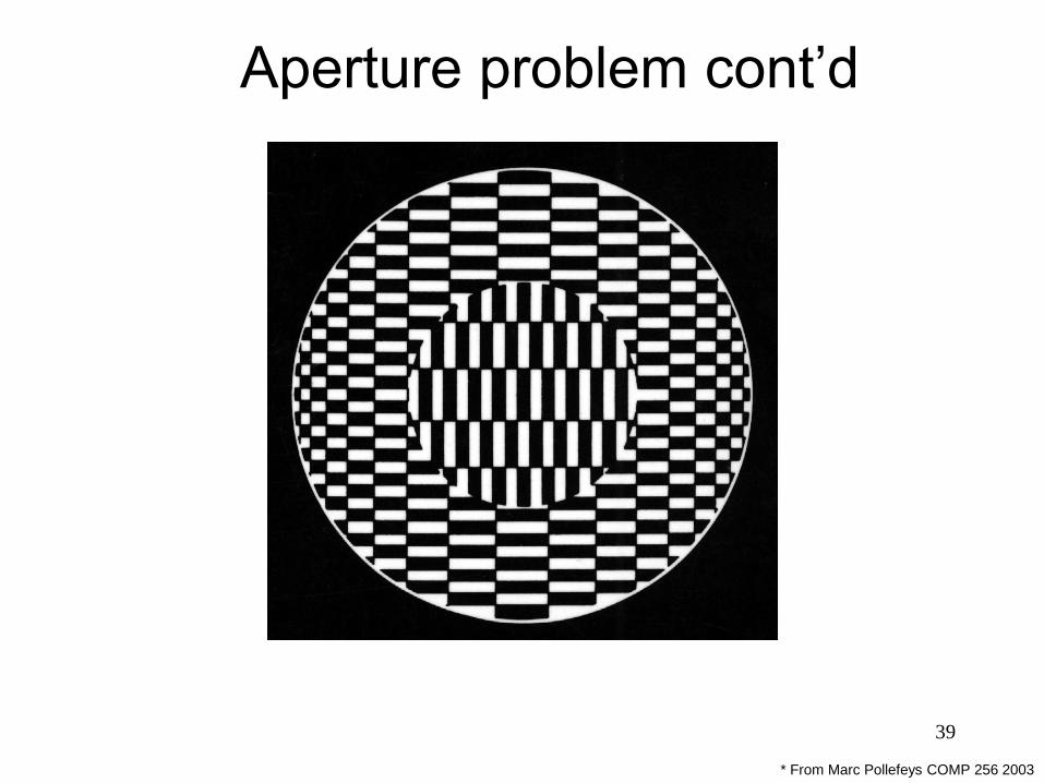
39

* From Marc Pollefeys COMP 256 2003

Aperture problem cont’d

Motion estimation techniques

Optical flow• Recover image motion at each pixel from spatio-temporal

image brightness variations (optical flow)

Feature-tracking• Extract visual features (corners, textured areas) and

“track” them over multiple frames

• Shi-Tomasi feature tracker

• Tracking with dynamics

• Implemented in Open CV

Tracking features

Courtesy of Jean-Yves Bouguet – Vision Lab, California Institute of Technology

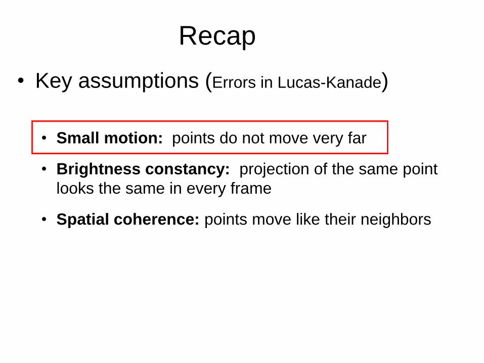
• Key assumptions (Errors in Lucas-Kanade)

• Small motion: points do not move very far

• Brightness constancy: projection of the same point

looks the same in every frame

• Spatial coherence: points move like their neighbors

Recap

Revisiting the small motion assumption

Is this motion small enough?• Probably not—it’s much larger than one pixel (2nd order terms dominate)

• How might we solve this problem?

* From Khurram Hassan-Shafique CAP5415 Computer Vision 2003

Reduce the resolution!

* From Khurram Hassan-Shafique CAP5415 Computer Vision 2003

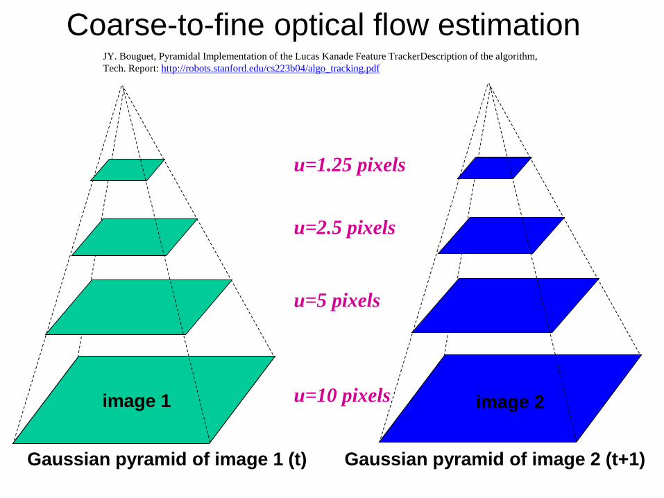
image Iimage H

Gaussian pyramid of image 1 (t) Gaussian pyramid of image 2 (t+1)

image 2image 1 u=10 pixels

u=5 pixels

u=2.5 pixels

u=1.25 pixels

Coarse-to-fine optical flow estimationJY. Bouguet, Pyramidal Implementation of the Lucas Kanade Feature TrackerDescription of the algorithm,

Tech. Report: http://robots.stanford.edu/cs223b04/algo_tracking.pdf

image Iimage J

Gaussian pyramid of image 1 (t) Gaussian pyramid of image 2 (t+1)

image 2image 1

run L-K

run L-K.

.

.

Coarse-to-fine optical flow estimationJY. Bouguet, Pyramidal Implementation of the Lucas Kanade Feature TrackerDescription of the algorithm,

Tech. Report: http://robots.stanford.edu/cs223b04/algo_tracking.pdf

Optical Flow Results

* From Khurram Hassan-Shafique CAP5415 Computer Vision 2003

Optical Flow Results

* From Khurram Hassan-Shafique CAP5415 Computer Vision 2003

• http://www.ces.clemson.edu/~stb/klt/

• OpenCV

• Key assumptions (Errors in Lucas-Kanade)

• Small motion: points do not move very far

• Brightness constancy: projection of the same point

looks the same in every frame

• Spatial coherence: points move like their neighbors

Recap

Motion segmentation

How do we represent the motion in this scene?

Break image sequence into “layers” each of which has a

coherent (affine) motion

Motion segmentationJ. Wang and E. Adelson. Layered Representation for Motion Analysis. CVPR 1993.

Substituting into the brightness

constancy equation:

yaxaayxv

yaxaayxu

654

321

),(

),(

0 tyx IvIuI

Affine motion

0)()( 654321 tyx IyaxaaIyaxaaI

Substituting into the brightness

constancy equation:

yaxaayxv

yaxaayxu

654

321

),(

),(

• Each pixel provides 1 linear constraint in

6 unknowns

2

tyx IyaxaaIyaxaaIaErr )()()( 654321

• If we have at least 6 pixels in a neighborhood,

a1… a6 can be found by least squares minimization:

Affine motion

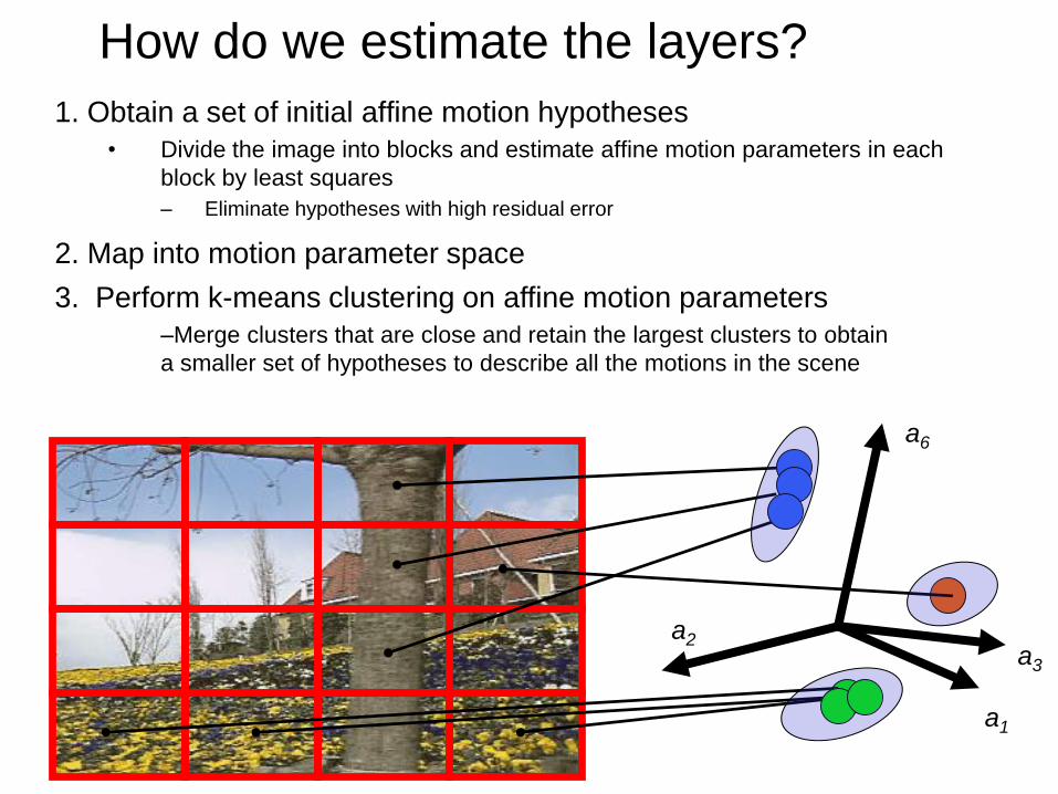
How do we estimate the layers?

1. Obtain a set of initial affine motion hypotheses

• Divide the image into blocks and estimate affine motion parameters in each

block by least squares

– Eliminate hypotheses with high residual error

2. Map into motion parameter space

3. Perform k-means clustering on affine motion parameters

–Merge clusters that are close and retain the largest clusters to obtain

a smaller set of hypotheses to describe all the motions in the scene

a1

a6

a2a3

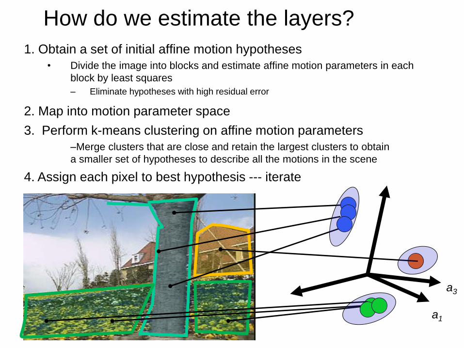
How do we estimate the layers?

1. Obtain a set of initial affine motion hypotheses

• Divide the image into blocks and estimate affine motion parameters in each

block by least squares

– Eliminate hypotheses with high residual error

2. Map into motion parameter space

3. Perform k-means clustering on affine motion parameters

–Merge clusters that are close and retain the largest clusters to obtain

a smaller set of hypotheses to describe all the motions in the scene

4. Assign each pixel to best hypothesis --- iterate

a1

a3

Example result

J. Wang and E. Adelson. Layered Representation for Motion Analysis. CVPR 1993.

CS231M · Mobile Computer Vision

Next lecture:

Neural networks and decision trees for machine vision