Lecture 6: Ohio University PHYS7501, Fall 2017, Z. Meisel (meisel@ohio.edu)

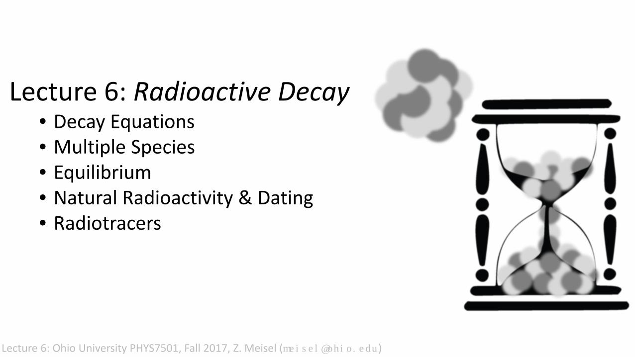
Lecture 6: Radioactive Decay• Decay Equations• Multiple Species• Equilibrium• Natural Radioactivity & Dating• Radiotracers

Radioactive Decay: Basic Concepts

2

•It is often energetically favorable for nuclei to undergo transmutation, either converting aproton to a neutron (or vice versa), emitting some combination of nucleons, or splitting apart.This is radioactive decay.

•Nuclei are effectively insulated from the surrounding environment and so the rate at which radioactive decay proceeds is independent of the surrounding conditions (e.g. pressure, temperature)

[Though, see the fascinating exception of bound-state β-decay in extremely high-temperature environments (J. Bachall, Phys. Rev. 1961)]

•In general, radioactive decay is an irreversible event[Again, sort of an exception in some exotic astrophysical environments, namely, Urca cycling (Gamow & Schoenberg, Phys. Rev. 1941)]

•Whether or not a particular nucleus undergoes decay depends on many stochastic processes,so the decay of several nucleons is described using statistical tools describing probability

•For large numbers of nuclei (pretty much every case: >1021 nuclei for a gram of almost anything), a statistical treatment is not only adequate, but also likely the only practicable way to describe decay kinetics

Decay Equations for One Nuclear Species• Since nuclear decay is (usually) independent of the surroundings, the rate at which a sample

composed of a particular isotope will undergo decay will just be proportional to the number of that isotope in the sample

• (𝐷𝐷𝐷𝐷𝐷𝐷𝐷𝐷𝐷𝐷 𝑅𝑅𝐷𝐷𝑅𝑅𝐷𝐷 𝑜𝑜𝑜𝑜 𝑆𝑆𝐷𝐷𝑆𝑆𝑆𝑆𝑆𝑆𝐷𝐷) ∝ (𝐷𝐷𝐷𝐷𝐷𝐷𝐷𝐷𝐷𝐷 𝑅𝑅𝐷𝐷𝑅𝑅𝐷𝐷 𝑜𝑜𝑜𝑜 𝑆𝑆𝑆𝑆𝑆𝑆𝑆𝑆𝑆𝑆𝐷𝐷 𝑁𝑁𝑁𝑁𝐷𝐷𝑆𝑆𝐷𝐷𝑁𝑁𝑁𝑁) × (𝑁𝑁𝑁𝑁𝑆𝑆𝑁𝑁𝐷𝐷𝑁𝑁 𝑜𝑜𝑜𝑜 𝑁𝑁𝑁𝑁𝐷𝐷𝑆𝑆𝐷𝐷𝑆𝑆)• A single nucleus will be no more or less likely to decay at one time as opposed to another,

so 𝐷𝐷𝐷𝐷𝐷𝐷𝐷𝐷𝐷𝐷 𝑅𝑅𝐷𝐷𝑅𝑅𝐷𝐷 𝑜𝑜𝑜𝑜 𝑆𝑆𝑆𝑆𝑆𝑆𝑆𝑆𝑆𝑆𝐷𝐷 𝑁𝑁𝑁𝑁𝐷𝐷𝑆𝑆𝐷𝐷𝑁𝑁𝑁𝑁 = 𝐷𝐷𝑜𝑜𝑆𝑆𝑁𝑁𝑅𝑅𝐷𝐷𝑆𝑆𝑅𝑅 ≡ λ• Therefore, the rate at which the sample decays,

i.e. the rate at which the number of nuclei 𝑁𝑁 decreases: −𝑑𝑑𝑑𝑑𝑑𝑑𝑑𝑑

= λ𝑁𝑁

• Keep in mind 𝑁𝑁 is changing with time, since decay is proceeding: −𝑑𝑑𝑑𝑑𝑑𝑑𝑑𝑑

= λ𝑁𝑁(𝑅𝑅)

• This is well and good, but we’re interested in 𝑁𝑁(𝑅𝑅), which isn’t obvious from the equation above

3

Decay Equations for One Nuclear Species• Solving for 𝑁𝑁(𝑅𝑅) from the seemingly innocuous equation 𝑑𝑑𝑑𝑑

𝑑𝑑𝑑𝑑= −λ𝑁𝑁(𝑅𝑅), is actually pretty hard,

unless one employs the Laplace transform, which turns our differential equation into an algebraic one

• For the LHS, we assume 𝑁𝑁(𝑅𝑅) to be an exponential function (empirically a safe bet) and use the derivative property of Laplace transform:

• 𝑑𝑑𝑑𝑑𝑑𝑑𝑑𝑑→ 𝑁𝑁𝑁𝑁 𝑁𝑁 − 𝑁𝑁(0)

• For the RHS, simply swap-in 𝑁𝑁 for time: −λ𝑁𝑁 𝑅𝑅 → −λ𝑁𝑁(𝑁𝑁)• Therefore, 𝑁𝑁𝑁𝑁(𝑁𝑁) − 𝑁𝑁(0) = −𝜆𝜆𝑁𝑁(𝑁𝑁)

• Which is re-written as: 𝑁𝑁 𝑁𝑁 = 𝑑𝑑(0)(𝑠𝑠+λ)

• Using one of several different methods (See E.g. D.Pressyanov, Am.J.Phys. 2002, or a Math Methods book),the inverse Laplace transform can be employed, yielding the familiar relation:

• 𝑁𝑁 𝑅𝑅 = 𝑁𝑁(0)𝐷𝐷−𝜆𝜆𝑑𝑑, the number of nuclei existing at time 𝑅𝑅• Since the Activity (decays/second) 𝐴𝐴 = 𝜆𝜆𝑁𝑁,

• 𝐴𝐴 𝑅𝑅 = 𝐴𝐴(0)𝐷𝐷−λ𝑑𝑑 4

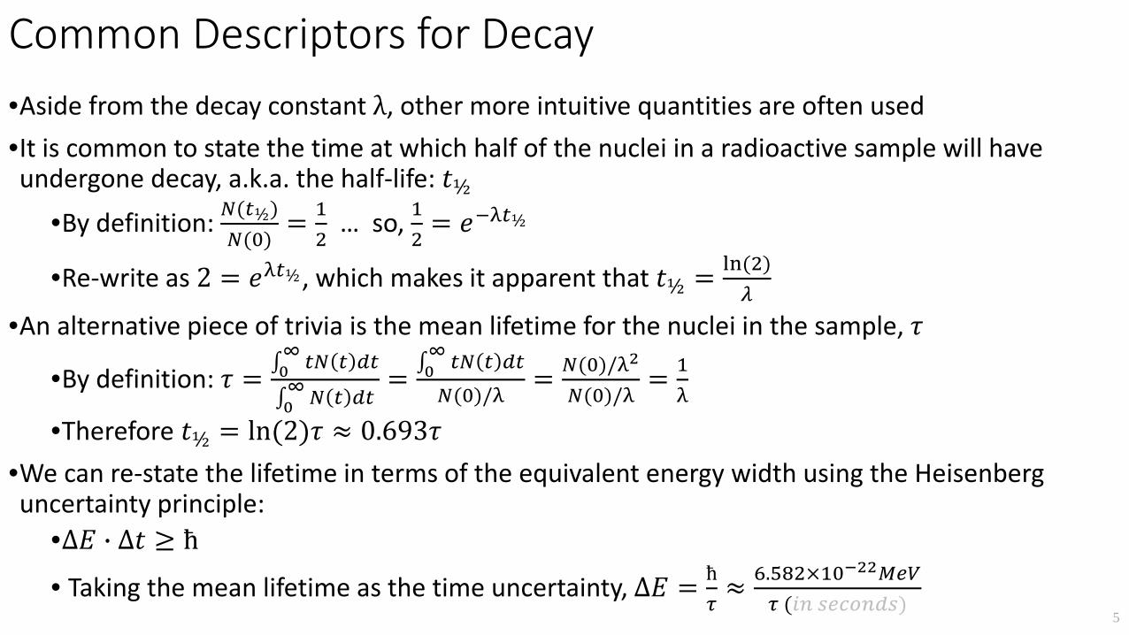
Common Descriptors for Decay •Aside from the decay constant λ, other more intuitive quantities are often used•It is common to state the time at which half of the nuclei in a radioactive sample will have undergone decay, a.k.a. the half-life: 𝑅𝑅½

•By definition: 𝑑𝑑(𝑑𝑑½)𝑑𝑑(0)

= 12

… so, 12

= 𝐷𝐷−λ𝑑𝑑½

•Re-write as 2 = 𝐷𝐷λ𝑑𝑑½ , which makes it apparent that 𝑅𝑅½ = ln(2)𝜆𝜆

•An alternative piece of trivia is the mean lifetime for the nuclei in the sample, 𝜏𝜏

•By definition: 𝜏𝜏 = ∫0∞ 𝑑𝑑𝑑𝑑 𝑑𝑑 𝑑𝑑𝑑𝑑

∫0∞ 𝑑𝑑 𝑑𝑑 𝑑𝑑𝑑𝑑

= ∫0∞ 𝑑𝑑𝑑𝑑 𝑑𝑑 𝑑𝑑𝑑𝑑𝑑𝑑(0)/λ

= 𝑑𝑑(0)/λ2

𝑑𝑑(0)/λ= 1

λ

•Therefore 𝑅𝑅½ = ln(2)𝜏𝜏 ≈ 0.693𝜏𝜏•We can re-state the lifetime in terms of the equivalent energy width using the Heisenberg uncertainty principle:

•∆𝐸𝐸 � ∆𝑅𝑅 ≥ ћ

• Taking the mean lifetime as the time uncertainty, ∆𝐸𝐸 = ћ𝜏𝜏≈ 6.582×10−22𝑀𝑀𝑀𝑀𝑀𝑀

𝜏𝜏 (𝑖𝑖𝑖𝑖 𝑠𝑠𝑀𝑀𝑠𝑠𝑠𝑠𝑖𝑖𝑑𝑑𝑠𝑠)5

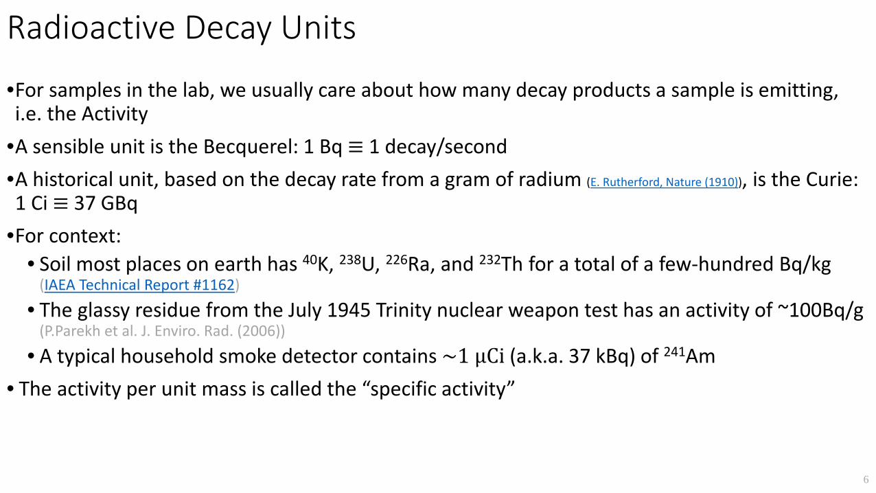
Radioactive Decay Units

•For samples in the lab, we usually care about how many decay products a sample is emitting,i.e. the Activity

•A sensible unit is the Becquerel: 1 Bq ≡ 1 decay/second•A historical unit, based on the decay rate from a gram of radium (E. Rutherford, Nature (1910)), is the Curie: 1 Ci ≡ 37 GBq

•For context:• Soil most places on earth has 40K, 238U, 226Ra, and 232Th for a total of a few-hundred Bq/kg

(IAEA Technical Report #1162)

• The glassy residue from the July 1945 Trinity nuclear weapon test has an activity of ~100Bq/g(P.Parekh et al. J. Enviro. Rad. (2006))

• A typical household smoke detector contains ~1 µCi (a.k.a. 37 kBq) of 241Am• The activity per unit mass is called the “specific activity”

6

7

Who uses “Curie”?

Burma

Liberia

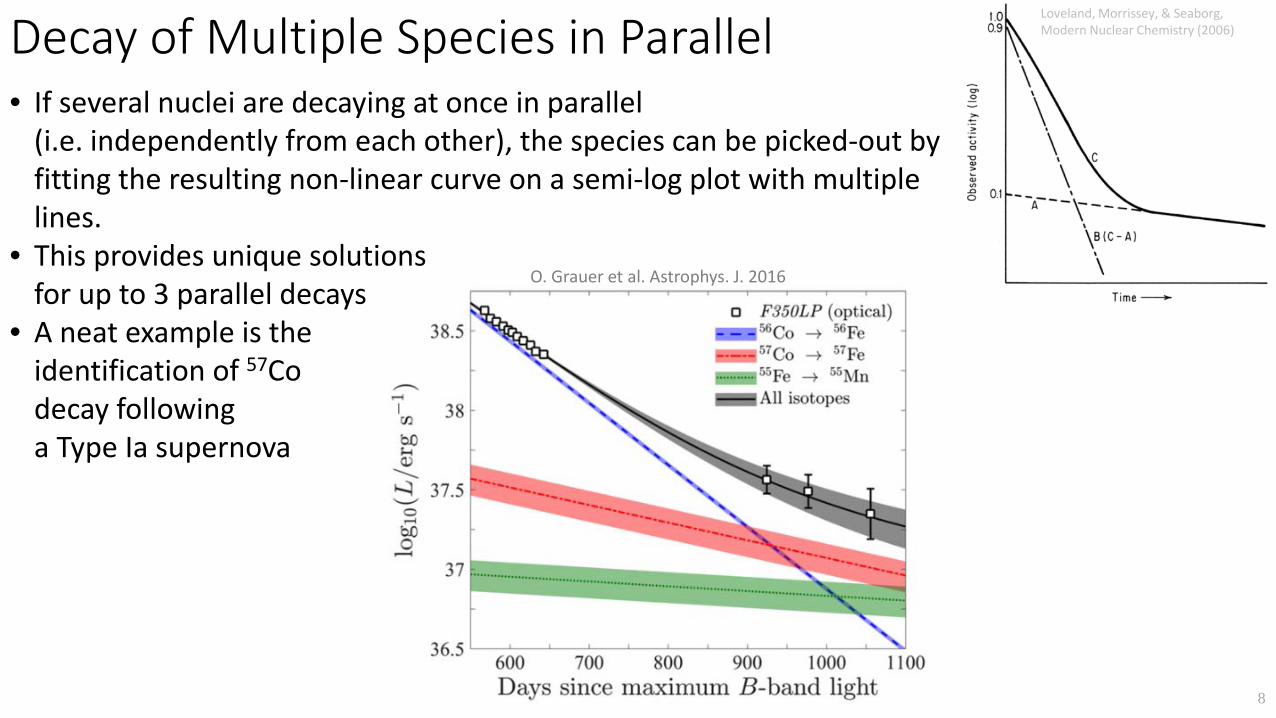
Decay of Multiple Species in Parallel

8

• If several nuclei are decaying at once in parallel(i.e. independently from each other), the species can be picked-out by fitting the resulting non-linear curve on a semi-log plot with multiple lines.

• This provides unique solutionsfor up to 3 parallel decays

• A neat example is theidentification of 57Codecay followinga Type Ia supernova

Loveland, Morrissey, & Seaborg,Modern Nuclear Chemistry (2006)

O. Grauer et al. Astrophys. J. 2016

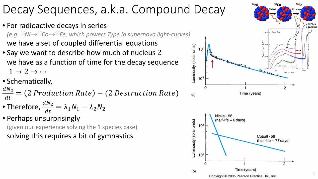
Decay Sequences, a.k.a. Compound Decay

9

• For radioactive decays in series (e.g. 56Ni→56Co→56Fe, which powers Type Ia supernova light-curves)we have a set of coupled differential equations

• Say we want to describe how much of nucleus 2we have as a function of time for the decay sequence1 → 2 → ⋯

• Schematically,𝑑𝑑𝑑𝑑2𝑑𝑑𝑑𝑑

= 2 𝑃𝑃𝑁𝑁𝑜𝑜𝑃𝑃𝑁𝑁𝐷𝐷𝑅𝑅𝑆𝑆𝑜𝑜𝑆𝑆 𝑅𝑅𝐷𝐷𝑅𝑅𝐷𝐷 − (2 𝐷𝐷𝐷𝐷𝑁𝑁𝑅𝑅𝑁𝑁𝑁𝑁𝐷𝐷𝑅𝑅𝑆𝑆𝑜𝑜𝑆𝑆 𝑅𝑅𝐷𝐷𝑅𝑅𝐷𝐷)

• Therefore, 𝑑𝑑𝑑𝑑2𝑑𝑑𝑑𝑑

= λ1𝑁𝑁1 − λ2𝑁𝑁2• Perhaps unsurprisingly

(given our experience solving the 1 species case)solving this requires a bit of gymnastics

MPA-Garching

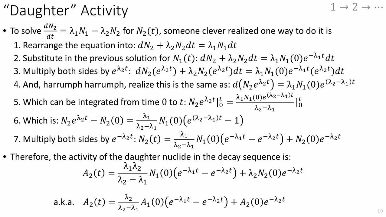
“Daughter” Activity• To solve 𝑑𝑑𝑑𝑑2

𝑑𝑑𝑑𝑑= λ1𝑁𝑁1 − λ2𝑁𝑁2 for 𝑁𝑁2(𝑅𝑅), someone clever realized one way to do it is

1. Rearrange the equation into: 𝑃𝑃𝑁𝑁2 + λ2𝑁𝑁2𝑃𝑃𝑅𝑅 = λ1𝑁𝑁1𝑃𝑃𝑅𝑅2. Substitute in the previous solution for 𝑁𝑁1(𝑅𝑅): 𝑃𝑃𝑁𝑁2 + λ2𝑁𝑁2𝑃𝑃𝑅𝑅 = λ1𝑁𝑁1(0)𝐷𝐷−λ1𝑑𝑑𝑃𝑃𝑅𝑅3. Multiply both sides by 𝐷𝐷λ2𝑑𝑑: 𝑃𝑃𝑁𝑁2(𝐷𝐷λ2𝑑𝑑) + λ2𝑁𝑁2(𝐷𝐷λ2𝑑𝑑)𝑃𝑃𝑅𝑅 = λ1𝑁𝑁1(0)𝐷𝐷−λ1𝑑𝑑(𝐷𝐷λ2𝑑𝑑)𝑃𝑃𝑅𝑅4. And, harrumph harrumph, realize this is the same as: 𝑃𝑃 𝑁𝑁2𝐷𝐷λ2𝑑𝑑 = λ1𝑁𝑁1(0)𝐷𝐷 λ2−λ1 𝑑𝑑

5. Which can be integrated from time 0 to 𝑅𝑅: 𝑁𝑁2𝐷𝐷λ2𝑑𝑑|0𝑑𝑑 = λ1𝑑𝑑1(0)𝑀𝑀 λ2−λ1 𝑡𝑡

λ2−λ1|0𝑑𝑑

6. Which is: 𝑁𝑁2𝐷𝐷λ2𝑑𝑑 − 𝑁𝑁2 0 = λ1λ2−λ1

𝑁𝑁1(0) 𝐷𝐷 λ2−λ1 𝑑𝑑 − 1

7. Multiply both sides by 𝐷𝐷−λ2𝑑𝑑: 𝑁𝑁2 𝑅𝑅 = λ1λ2−λ1

𝑁𝑁1 0 𝐷𝐷−λ1𝑑𝑑 − 𝐷𝐷−λ2𝑑𝑑 + 𝑁𝑁2(0)𝐷𝐷−λ2𝑑𝑑

• Therefore, the activity of the daughter nuclide in the decay sequence is:

𝐴𝐴2 𝑅𝑅 =λ1λ2λ2 − λ1

𝑁𝑁1 0 𝐷𝐷−λ1𝑑𝑑 − 𝐷𝐷−λ2𝑑𝑑 + λ2𝑁𝑁2 0 𝐷𝐷−λ2𝑑𝑑

a.k.a. 𝐴𝐴2 𝑅𝑅 = λ2λ2−λ1

𝐴𝐴1 0 𝐷𝐷−λ1𝑑𝑑 − 𝐷𝐷−λ2𝑑𝑑 + 𝐴𝐴2 0 𝐷𝐷−λ2𝑑𝑑10

1 → 2 → ⋯

“Daughter” Activity

11

1 → 2 → ⋯

𝐴𝐴2 𝑅𝑅 =λ2

λ2 − λ1𝐴𝐴1 0 𝐷𝐷−λ1𝑑𝑑 − 𝐷𝐷−λ2𝑑𝑑 + 𝐴𝐴2 0 𝐷𝐷−λ2𝑑𝑑

P

Loveland, Morrissey, & Seaborg,Modern Nuclear Chemistry (2006)

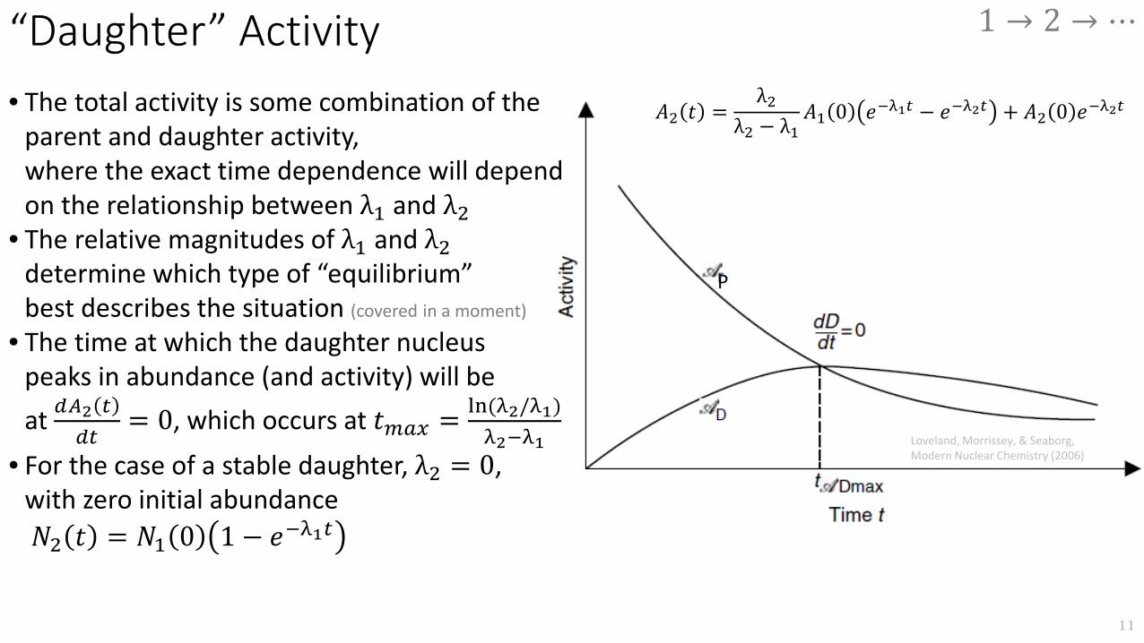
• The total activity is some combination of the parent and daughter activity,where the exact time dependence will depend on the relationship between λ1 and λ2

• The relative magnitudes of λ1 and λ2determine which type of “equilibrium”best describes the situation (covered in a moment)

• The time at which the daughter nucleuspeaks in abundance (and activity) will beat 𝑑𝑑𝐴𝐴2 𝑑𝑑

𝑑𝑑𝑑𝑑= 0, which occurs at 𝑅𝑅𝑚𝑚𝑚𝑚𝑚𝑚 = ln(λ2/λ1)

λ2−λ1• For the case of a stable daughter, λ2 = 0,

with zero initial abundance𝑁𝑁2 𝑅𝑅 = 𝑁𝑁1 0 1 − 𝐷𝐷−λ1𝑑𝑑

P P

P

P

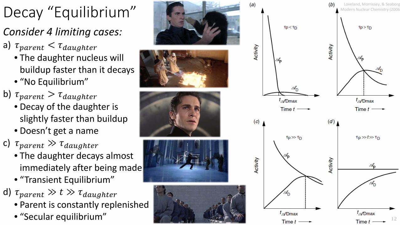
Decay “Equilibrium”

12

Consider 4 limiting cases:a) 𝜏𝜏𝑝𝑝𝑚𝑚𝑝𝑝𝑀𝑀𝑖𝑖𝑑𝑑 < 𝜏𝜏𝑑𝑑𝑚𝑚𝑑𝑑𝑑𝑑𝑑𝑑𝑑𝑀𝑀𝑝𝑝

• The daughter nucleus willbuildup faster than it decays

• “No Equilibrium”b) 𝜏𝜏𝑝𝑝𝑚𝑚𝑝𝑝𝑀𝑀𝑖𝑖𝑑𝑑 > 𝜏𝜏𝑑𝑑𝑚𝑚𝑑𝑑𝑑𝑑𝑑𝑑𝑑𝑀𝑀𝑝𝑝

• Decay of the daughter isslightly faster than buildup

• Doesn’t get a namec) 𝜏𝜏𝑝𝑝𝑚𝑚𝑝𝑝𝑀𝑀𝑖𝑖𝑑𝑑 ≫ 𝜏𝜏𝑑𝑑𝑚𝑚𝑑𝑑𝑑𝑑𝑑𝑑𝑑𝑀𝑀𝑝𝑝

• The daughter decays almostimmediately after being made

• “Transient Equilibrium”d) 𝜏𝜏𝑝𝑝𝑚𝑚𝑝𝑝𝑀𝑀𝑖𝑖𝑑𝑑 ≫ 𝑅𝑅 ≫ 𝜏𝜏𝑑𝑑𝑚𝑚𝑑𝑑𝑑𝑑𝑑𝑑𝑑𝑀𝑀𝑝𝑝

• Parent is constantly replenished• “Secular equilibrium”

Loveland, Morrissey, & Seaborg, Modern Nuclear Chemistry (2006)

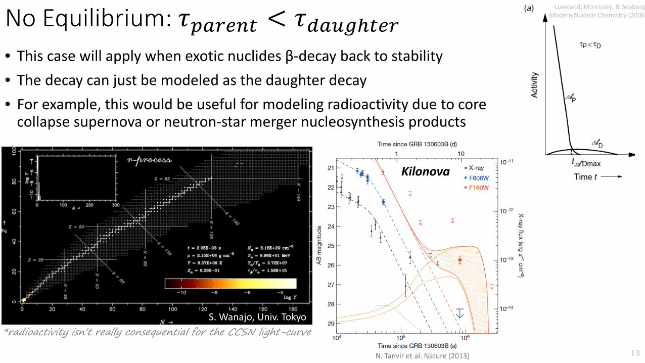
No Equilibrium: 𝜏𝜏𝑝𝑝𝑚𝑚𝑝𝑝𝑀𝑀𝑖𝑖𝑑𝑑 < 𝜏𝜏𝑑𝑑𝑚𝑚𝑑𝑑𝑑𝑑𝑑𝑑𝑑𝑀𝑀𝑝𝑝• This case will apply when exotic nuclides β-decay back to stability• The decay can just be modeled as the daughter decay• For example, this would be useful for modeling radioactivity due to core

collapse supernova or neutron-star merger nucleosynthesis products

13

P

Loveland, Morrissey, & Seaborg, Modern Nuclear Chemistry (2006)

Kilonova

N. Tanvir et al. Nature (2013)

S. Wanajo, Univ. Tokyo*radioactivity isn’t really consequential for the CCSN light-curve

Loveland, Morrissey, & Seaborg, Modern Nuclear Chemistry (2006)

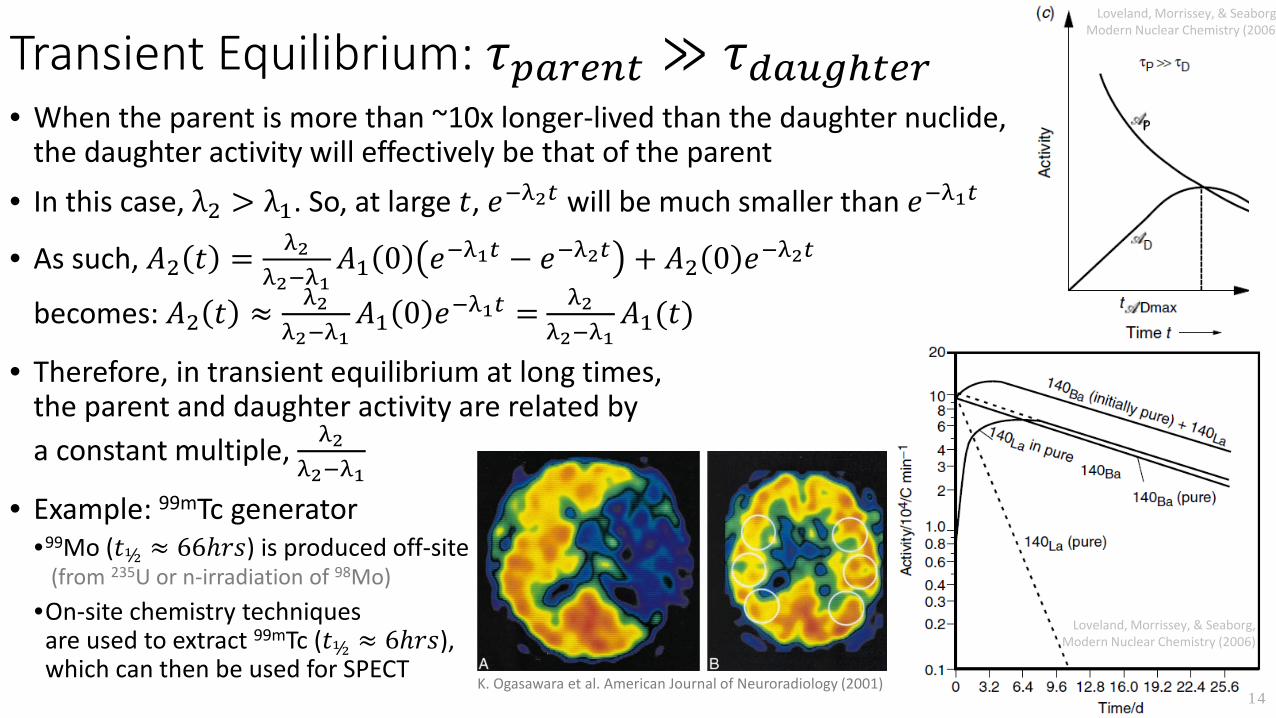
Transient Equilibrium: 𝜏𝜏𝑝𝑝𝑚𝑚𝑝𝑝𝑀𝑀𝑖𝑖𝑑𝑑 ≫ 𝜏𝜏𝑑𝑑𝑚𝑚𝑑𝑑𝑑𝑑𝑑𝑑𝑑𝑀𝑀𝑝𝑝• When the parent is more than ~10x longer-lived than the daughter nuclide,

the daughter activity will effectively be that of the parent• In this case, λ2 > λ1. So, at large 𝑅𝑅, 𝐷𝐷−λ2𝑑𝑑 will be much smaller than 𝐷𝐷−λ1𝑑𝑑

• As such, 𝐴𝐴2 𝑅𝑅 = λ2λ2−λ1

𝐴𝐴1 0 𝐷𝐷−λ1𝑑𝑑 − 𝐷𝐷−λ2𝑑𝑑 + 𝐴𝐴2 0 𝐷𝐷−λ2𝑑𝑑

becomes: 𝐴𝐴2 𝑅𝑅 ≈ λ2λ2−λ1

𝐴𝐴1 0 𝐷𝐷−λ1𝑑𝑑 = λ2λ2−λ1

𝐴𝐴1(𝑅𝑅)

• Therefore, in transient equilibrium at long times,the parent and daughter activity are related bya constant multiple, λ2

λ2−λ1• Example: 99mTc generator

•99Mo (𝑅𝑅½ ≈ 66ℎ𝑁𝑁𝑁𝑁) is produced off-site(from 235U or n-irradiation of 98Mo)

•On-site chemistry techniquesare used to extract 99mTc (𝑅𝑅½ ≈ 6ℎ𝑁𝑁𝑁𝑁),which can then be used for SPECT

14

P

Loveland, Morrissey, & Seaborg, Modern Nuclear Chemistry (2006)

K. Ogasawara et al. American Journal of Neuroradiology (2001)

P

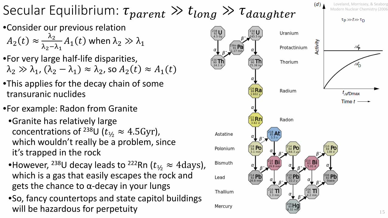
Secular Equilibrium: 𝜏𝜏𝑝𝑝𝑚𝑚𝑝𝑝𝑀𝑀𝑖𝑖𝑑𝑑 ≫ 𝑅𝑅𝑙𝑙𝑠𝑠𝑖𝑖𝑑𝑑 ≫ 𝜏𝜏𝑑𝑑𝑚𝑚𝑑𝑑𝑑𝑑𝑑𝑑𝑑𝑀𝑀𝑝𝑝•Consider our previous relation𝐴𝐴2 𝑅𝑅 ≈ λ2

λ2−λ1𝐴𝐴1 𝑅𝑅 when λ2 ≫ λ1

•For very large half-life disparities,λ2 ≫ λ1, (λ2 − λ1) ≈ λ2, so 𝐴𝐴2 𝑅𝑅 ≈ 𝐴𝐴1(𝑅𝑅)

•This applies for the decay chain of sometransuranic nuclides

•For example: Radon from Granite•Granite has relatively largeconcentrations of 238U (𝑅𝑅½ ≈ 4.5Gyr),which wouldn’t really be a problem, sinceit’s trapped in the rock

•However, 238U decay leads to 222Rn (𝑅𝑅½ ≈ 4days),which is a gas that easily escapes the rock andgets the chance to α-decay in your lungs

•So, fancy countertops and state capitol buildingswill be hazardous for perpetuity 15

Loveland, Morrissey, & Seaborg, Modern Nuclear Chemistry (2006)

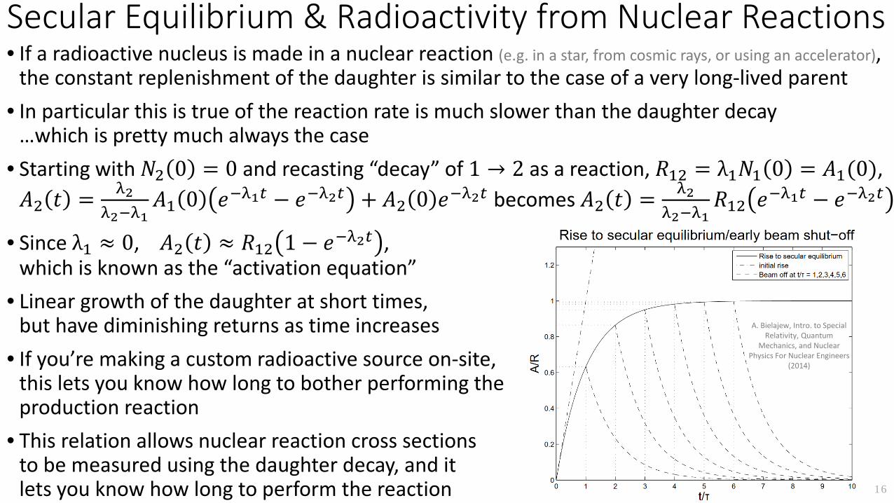
Secular Equilibrium & Radioactivity from Nuclear Reactions• If a radioactive nucleus is made in a nuclear reaction (e.g. in a star, from cosmic rays, or using an accelerator),

the constant replenishment of the daughter is similar to the case of a very long-lived parent• In particular this is true of the reaction rate is much slower than the daughter decay

…which is pretty much always the case• Starting with 𝑁𝑁2 0 = 0 and recasting “decay” of 1 → 2 as a reaction, 𝑅𝑅12 = λ1𝑁𝑁1 0 = 𝐴𝐴1(0),𝐴𝐴2 𝑅𝑅 = λ2

λ2−λ1𝐴𝐴1 0 𝐷𝐷−λ1𝑑𝑑 − 𝐷𝐷−λ2𝑑𝑑 + 𝐴𝐴2 0 𝐷𝐷−λ2𝑑𝑑 becomes 𝐴𝐴2 𝑅𝑅 = λ2

λ2−λ1𝑅𝑅12 𝐷𝐷−λ1𝑑𝑑 − 𝐷𝐷−λ2𝑑𝑑

• Since λ1 ≈ 0, 𝐴𝐴2 𝑅𝑅 ≈ 𝑅𝑅12 1 − 𝐷𝐷−λ2𝑑𝑑 ,which is known as the “activation equation”

• Linear growth of the daughter at short times,but have diminishing returns as time increases

• If you’re making a custom radioactive source on-site,this lets you know how long to bother performing theproduction reaction

• This relation allows nuclear reaction cross sectionsto be measured using the daughter decay, and itlets you know how long to perform the reaction 16

A. Bielajew, Intro. to Special Relativity, Quantum

Mechanics, and Nuclear Physics For Nuclear Engineers

(2014)

Reaction Cross Section Measurements with Activation• Assuming the decay of the daughter nucleus is understood, the reaction rate for the production

reaction is extracted from 𝑅𝑅12 = 𝐴𝐴2 𝑅𝑅 / 1 − 𝐷𝐷−λ2𝑑𝑑

• After performing the reaction 1 → 2 for time 𝑅𝑅𝑖𝑖𝑝𝑝𝑝𝑝 and then measuring the activity 𝐴𝐴2(𝑅𝑅𝑖𝑖𝑝𝑝𝑝𝑝), 𝑅𝑅12 = 𝐴𝐴2(𝑑𝑑𝑖𝑖𝑖𝑖𝑖𝑖)𝑀𝑀−λ2𝑡𝑡𝑖𝑖𝑖𝑖𝑖𝑖

1−𝑀𝑀−λ2𝑡𝑡𝑖𝑖𝑖𝑖𝑖𝑖

• The rate of production 𝑅𝑅12 is related to the reaction probability, the “cross section”, by𝑃𝑃𝑁𝑁𝑜𝑜𝑃𝑃𝑁𝑁𝐷𝐷𝑅𝑅𝑆𝑆𝑜𝑜𝑆𝑆 𝑅𝑅𝐷𝐷𝑅𝑅𝐷𝐷 = # 𝐼𝐼𝑆𝑆𝐷𝐷𝑆𝑆𝑃𝑃𝐷𝐷𝑆𝑆𝑅𝑅 𝑁𝑁𝑁𝑁𝐷𝐷𝑆𝑆𝐷𝐷𝑆𝑆 ∗ 𝐴𝐴𝐷𝐷𝑁𝑁𝑆𝑆𝐷𝐷𝑆𝑆 𝑁𝑁𝑁𝑁𝑆𝑆𝑁𝑁𝐷𝐷𝑁𝑁 𝐷𝐷𝐷𝐷𝑆𝑆𝑁𝑁𝑆𝑆𝑅𝑅𝐷𝐷 𝑜𝑜𝑜𝑜 𝑇𝑇𝐷𝐷𝑁𝑁𝑆𝑆𝐷𝐷𝑅𝑅 𝑁𝑁𝑁𝑁𝐷𝐷𝑆𝑆𝐷𝐷𝑆𝑆 ∗ (𝐶𝐶𝑁𝑁𝑜𝑜𝑁𝑁𝑁𝑁 𝑆𝑆𝐷𝐷𝐷𝐷𝑅𝑅𝑆𝑆𝑜𝑜𝑆𝑆)

• 𝑅𝑅12 = 𝑁𝑁1𝑆𝑆2𝜎𝜎12• So, once we’ve counted the number of projectiles, determined the aerial target density,

measured the activity and irradiation time, and taken into account detection efficiencies and time delays between activity measurements and the end of irradiation

•𝜎𝜎12 = 𝐴𝐴2(𝑑𝑑𝑖𝑖𝑖𝑖𝑖𝑖)𝑀𝑀−λ2𝑡𝑡𝑖𝑖𝑖𝑖𝑖𝑖

𝑑𝑑1𝑖𝑖2 1−𝑀𝑀−λ2𝑡𝑡𝑖𝑖𝑖𝑖𝑖𝑖

17

One pit-fall is a lack of knowledge about the daughter decay due to unaccounted for decay branches.For a detailed discussion of other complications, see e.g. G.Kiss et al. Phys. Lett. B (2014)

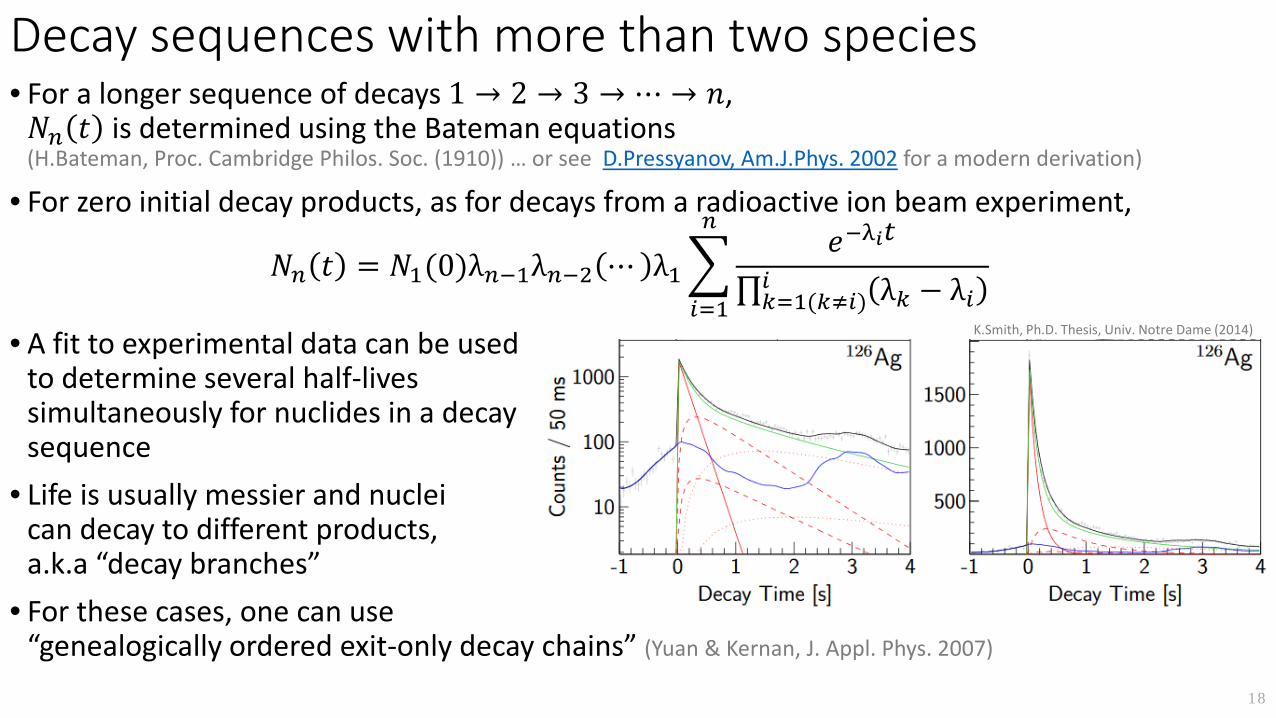
Decay sequences with more than two species• For a longer sequence of decays 1 → 2 → 3 → ⋯ → 𝑆𝑆,𝑁𝑁𝑖𝑖 𝑅𝑅 is determined using the Bateman equations(H.Bateman, Proc. Cambridge Philos. Soc. (1910)) … or see D.Pressyanov, Am.J.Phys. 2002 for a modern derivation)

• For zero initial decay products, as for decays from a radioactive ion beam experiment,

𝑁𝑁𝑖𝑖 𝑅𝑅 = 𝑁𝑁1(0)λ𝑖𝑖−1λ𝑖𝑖−2 ⋯ λ1�𝑖𝑖=1

𝑖𝑖𝐷𝐷−λ𝑖𝑖𝑑𝑑

∏𝑘𝑘=1(𝑘𝑘≠𝑖𝑖)𝑖𝑖 λ𝑘𝑘 − λ𝑖𝑖

• A fit to experimental data can be usedto determine several half-livessimultaneously for nuclides in a decaysequence

• Life is usually messier and nucleican decay to different products,a.k.a “decay branches”

• For these cases, one can use“genealogically ordered exit-only decay chains” (Yuan & Kernan, J. Appl. Phys. 2007)

18

K.Smith, Ph.D. Thesis, Univ. Notre Dame (2014)

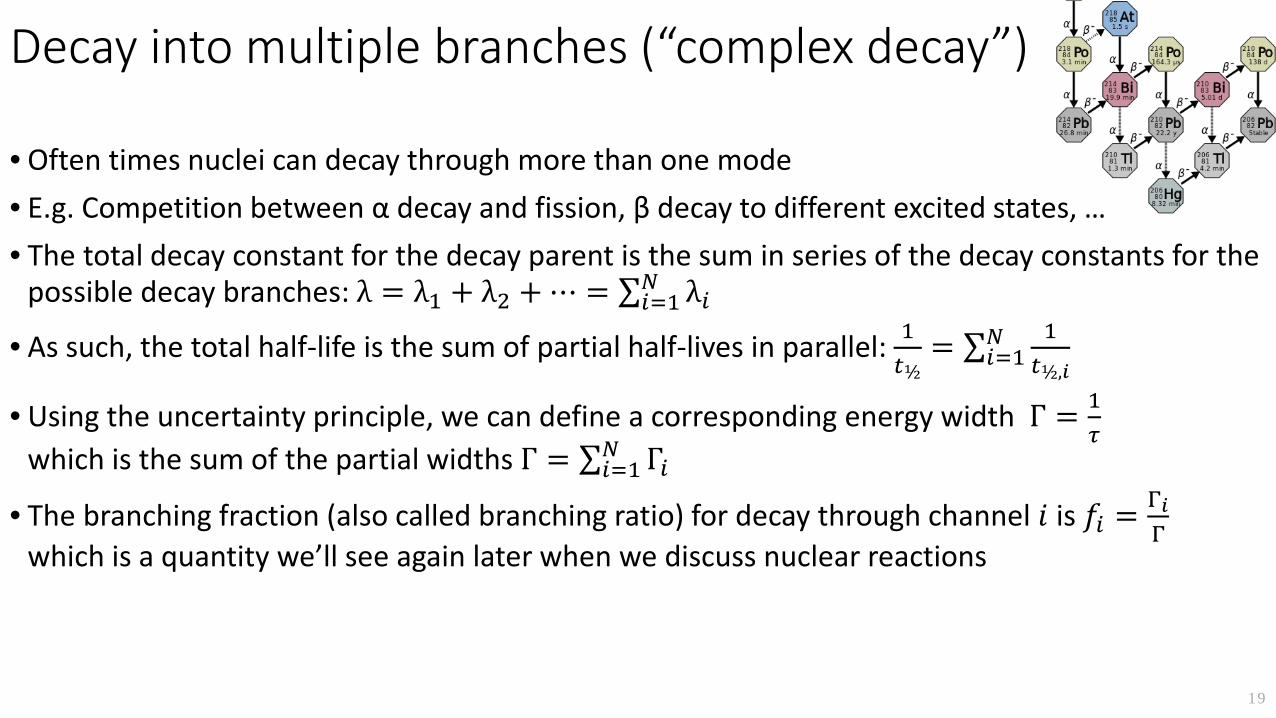
Decay into multiple branches (“complex decay”)

• Often times nuclei can decay through more than one mode• E.g. Competition between α decay and fission, β decay to different excited states, …• The total decay constant for the decay parent is the sum in series of the decay constants for the

possible decay branches: λ = λ1 + λ2 + ⋯ = ∑𝑖𝑖=1𝑑𝑑 λ𝑖𝑖• As such, the total half-life is the sum of partial half-lives in parallel: 1

𝑑𝑑½= ∑𝑖𝑖=1𝑑𝑑 1

𝑑𝑑½,𝑖𝑖

• Using the uncertainty principle, we can define a corresponding energy width Γ = 1𝜏𝜏

which is the sum of the partial widths Γ = ∑𝑖𝑖=1𝑑𝑑 Γ𝑖𝑖• The branching fraction (also called branching ratio) for decay through channel 𝑆𝑆 is 𝑜𝑜𝑖𝑖 = Γ𝑖𝑖

Γwhich is a quantity we’ll see again later when we discuss nuclear reactions

19

Arevalo Jr., McDonough, & Luong, Earth & Planetary Sci. Lett. (2009)

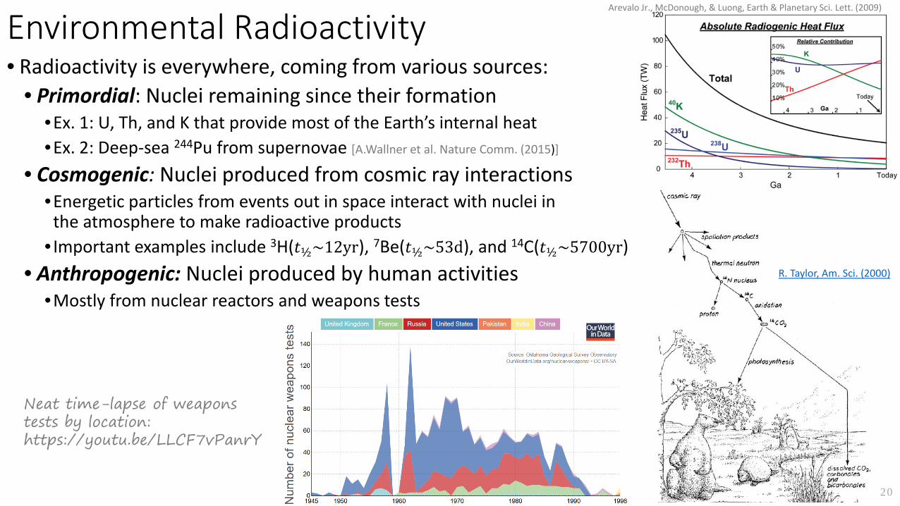
Environmental Radioactivity• Radioactivity is everywhere, coming from various sources:

• Primordial: Nuclei remaining since their formation •Ex. 1: U, Th, and K that provide most of the Earth’s internal heat•Ex. 2: Deep-sea 244Pu from supernovae [A.Wallner et al. Nature Comm. (2015)]

• Cosmogenic: Nuclei produced from cosmic ray interactions•Energetic particles from events out in space interact with nuclei in

the atmosphere to make radioactive products• Important examples include 3H(𝑅𝑅½~12yr), 7Be(𝑅𝑅½~53d), and 14C(𝑅𝑅½~5700yr)

• Anthropogenic: Nuclei produced by human activities•Mostly from nuclear reactors and weapons tests

20

R. Taylor, Am. Sci. (2000)

Neat time-lapse of weapons tests by location: https://youtu.be/LLCF7vPanrY

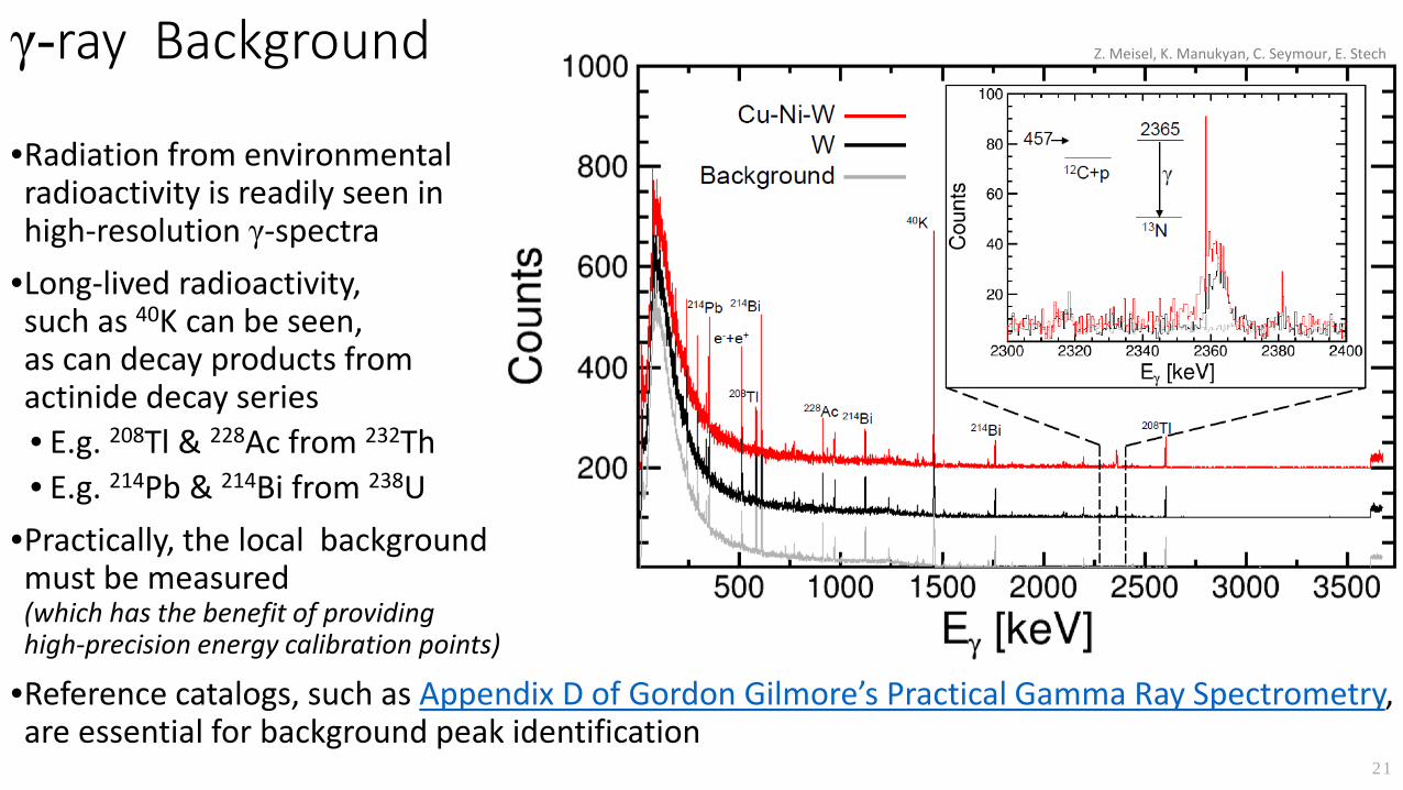
γ-ray Background

21

Z. Meisel, K. Manukyan, C. Seymour, E. Stech

•Radiation from environmentalradioactivity is readily seen inhigh-resolution γ-spectra

•Long-lived radioactivity,such as 40K can be seen,as can decay products fromactinide decay series • E.g. 208Tl & 228Ac from 232Th• E.g. 214Pb & 214Bi from 238U

•Practically, the local backgroundmust be measured(which has the benefit of providinghigh-precision energy calibration points)

•Reference catalogs, such as Appendix D of Gordon Gilmore’s Practical Gamma Ray Spectrometry, are essential for background peak identification

Radionuclide Dating

22

• If an object contains or contained a radioactive nucleus, we can use this to tell how old it is• From the equation for decay of a single species 𝑁𝑁 𝑅𝑅 = 𝑁𝑁(0)𝐷𝐷−𝜆𝜆/𝑑𝑑,

we can solve for the time 𝑅𝑅 =ln �𝑁𝑁(𝑡𝑡)

𝑁𝑁(0)

λ

• However, while determining 𝑁𝑁(𝑅𝑅) just requires counting (𝐴𝐴 𝑅𝑅 = λ𝑁𝑁(𝑅𝑅)),often we have no way to know 𝑁𝑁(0)

• The solution is to keep in mind that for the decay sequence, e.g. 1 → 2, the total number of nuclei in the decay sequence is constant: 𝑁𝑁1 𝑅𝑅 + 𝑁𝑁2 𝑅𝑅 = 𝑁𝑁𝑑𝑑𝑠𝑠𝑑𝑑 = 𝐷𝐷𝑜𝑜𝑆𝑆𝑁𝑁𝑅𝑅𝐷𝐷𝑆𝑆𝑅𝑅

• As such, assuming 𝑁𝑁2 0 = 0, then 𝑅𝑅 = 1λ

ln 1 + 𝑑𝑑2(𝑑𝑑)𝑑𝑑1(𝑑𝑑)

,so we only need the ratio of daughter to parent nuclides in the sample

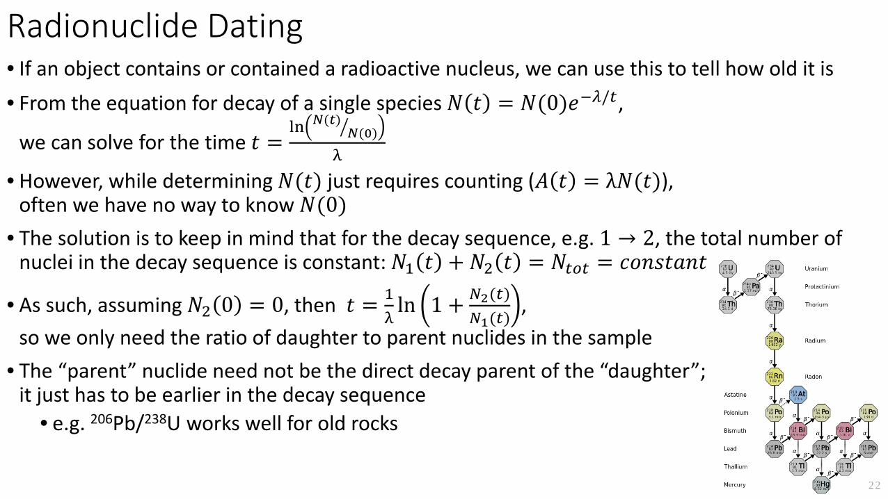
• The “parent” nuclide need not be the direct decay parent of the “daughter”;it just has to be earlier in the decay sequence

• e.g. 206Pb/238U works well for old rocks

Geochronometers• Since the assumption 𝑁𝑁2 0 = 0 often has to be relaxed, another trick has to be applied• If a stable isotope of the daughter element originally existed in the sample and isn’t formed by

the decay of something long-lived, then we at least know the ratio between the total number of nuclei in the decay chain to the number of nuclei of that stable isotope remained constant: 𝑑𝑑1 𝑑𝑑 +𝑑𝑑2(𝑑𝑑)

𝑑𝑑𝑠𝑠= 𝑑𝑑1 0 +𝑑𝑑2(0)

𝑑𝑑𝑠𝑠

• Since 𝑁𝑁1 0 = 𝑁𝑁1(𝑅𝑅)𝐷𝐷λ1𝑑𝑑, 𝑑𝑑2(𝑑𝑑)𝑑𝑑𝑠𝑠

= 𝑑𝑑2 0 +𝑑𝑑1(𝑑𝑑)(1+𝑀𝑀λ1𝑡𝑡)𝑑𝑑𝑠𝑠

• Plotting 𝑑𝑑2(𝑑𝑑)𝑑𝑑𝑠𝑠

vs 𝑑𝑑1(𝑑𝑑)𝑑𝑑𝑠𝑠

for a sequence of measurementscreates a straight line which 𝑁𝑁2(0) and 𝑅𝑅 can easily bedetermined from

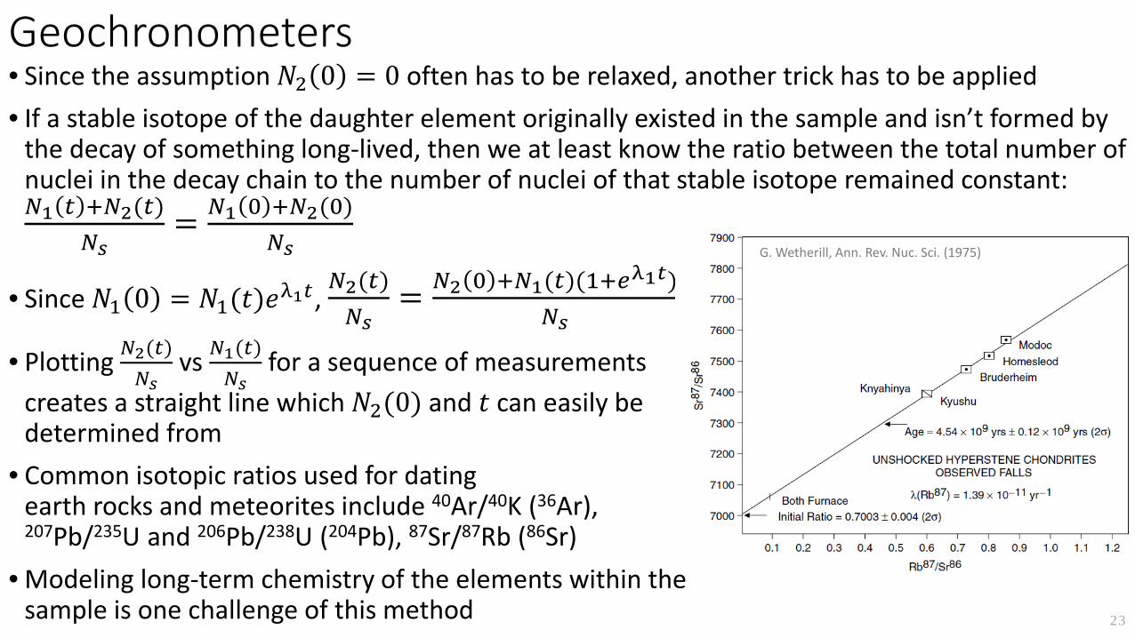
• Common isotopic ratios used for datingearth rocks and meteorites include 40Ar/40K (36Ar),207Pb/235U and 206Pb/238U (204Pb), 87Sr/87Rb (86Sr)

• Modeling long-term chemistry of the elements within thesample is one challenge of this method

G. Wetherill, Ann. Rev. Nuc. Sci. (1975)

23

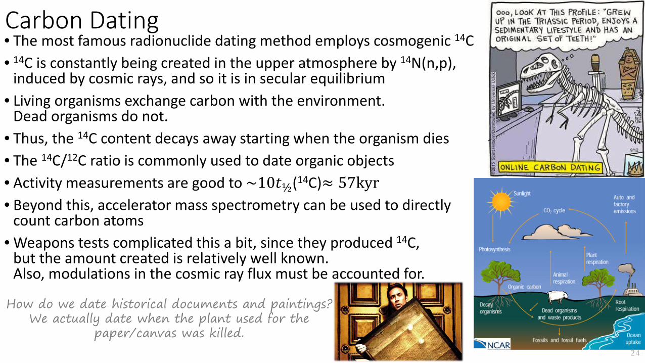
Carbon Dating• The most famous radionuclide dating method employs cosmogenic 14C • 14C is constantly being created in the upper atmosphere by 14N(n,p),

induced by cosmic rays, and so it is in secular equilibrium• Living organisms exchange carbon with the environment.

Dead organisms do not.• Thus, the 14C content decays away starting when the organism dies• The 14C/12C ratio is commonly used to date organic objects• Activity measurements are good to ~10𝑅𝑅½(14C)≈ 57kyr• Beyond this, accelerator mass spectrometry can be used to directly

count carbon atoms• Weapons tests complicated this a bit, since they produced 14C,

but the amount created is relatively well known.Also, modulations in the cosmic ray flux must be accounted for.

24

How do we date historical documents and paintings?We actually date when the plant used for the

paper/canvas was killed.

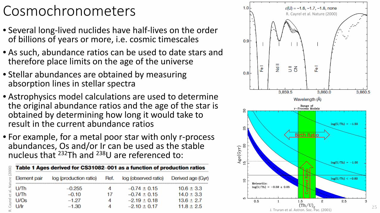
Cosmochronometers• Several long-lived nuclides have half-lives on the order

of billions of years or more, i.e. cosmic timescales• As such, abundance ratios can be used to date stars and

therefore place limits on the age of the universe• Stellar abundances are obtained by measuring

absorption lines in stellar spectra• Astrophysics model calculations are used to determine

the original abundance ratios and the age of the star is obtained by determining how long it would take to result in the current abundance ratios

• For example, for a metal poor star with only r-process abundances, Os and/or Ir can be used as the stable nucleus that 232Th and 238U are referenced to:

25

R. Cayrel et al. Nature (2000)R.

Cay

rele

t al.

Nat

ure

(200

0)

J. Truran et al. Astron. Soc. Pac. (2001)

Curr

ent R

atio

Birth Ratio

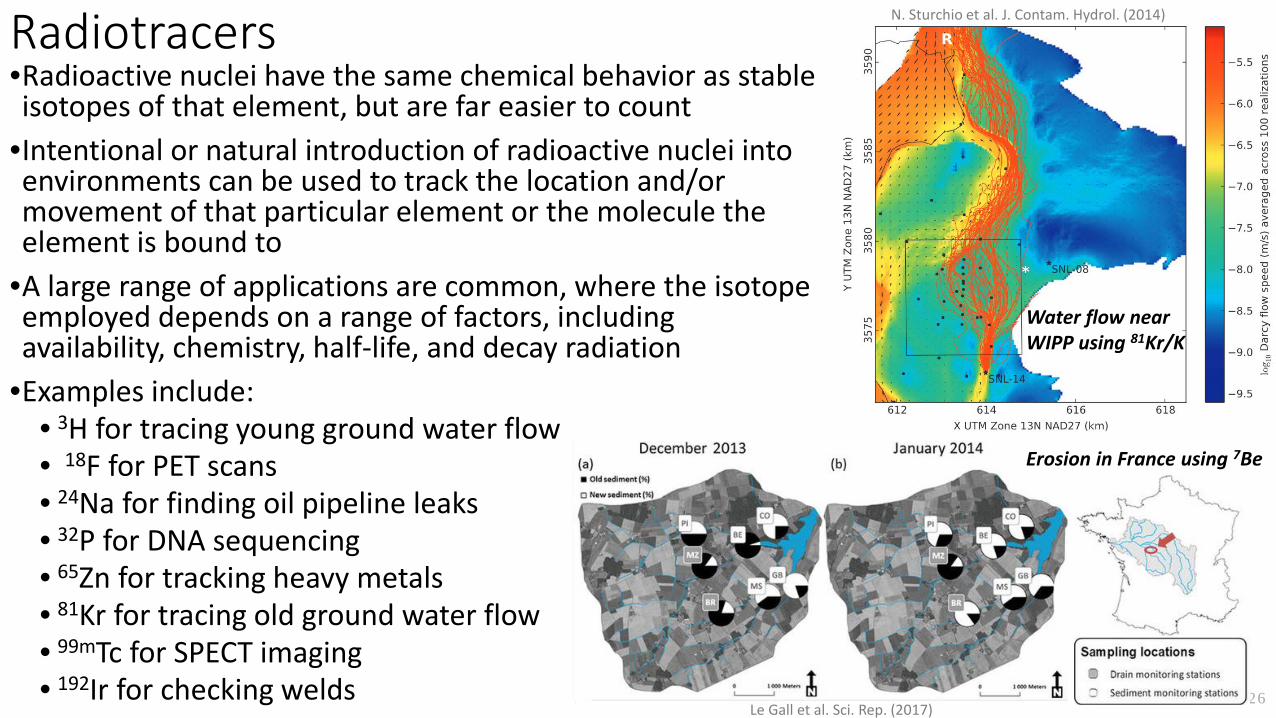
Radiotracers•Radioactive nuclei have the same chemical behavior as stable isotopes of that element, but are far easier to count

•Intentional or natural introduction of radioactive nuclei into environments can be used to track the location and/or movement of that particular element or the molecule the element is bound to

•A large range of applications are common, where the isotope employed depends on a range of factors, including availability, chemistry, half-life, and decay radiation

•Examples include:• 3H for tracing young ground water flow• 18F for PET scans• 24Na for finding oil pipeline leaks• 32P for DNA sequencing• 65Zn for tracking heavy metals• 81Kr for tracing old ground water flow• 99mTc for SPECT imaging• 192Ir for checking welds 26

Water flow near WIPP using 81Kr/K

N. Sturchio et al. J. Contam. Hydrol. (2014)

Erosion in France using 7Be

Le Gall et al. Sci. Rep. (2017)

Further Reading• Chapters 3 & 4: Modern Nuclear Chemistry (Loveland, Morrissey, Seaborg)• Chapter 2: Nuclear & Particle Physics (B.R. Martin)• Chapter 14, Section 6: Quantum Mechanics for Engineers (L. van Dommelen)• Chapter 5: Mathematics for Physicists (S. Lea)• Chapter 13: Introduction to Special Relativity, Quantum Mechanics, and Nuclear Physics for

Nuclear Engineers (A. Bielajew)

27