lecture 3 ‘linear’ transverse...

Lecture 3 ‘Linear’ Transverse Dynamics

(Ch. 3 of FOBP, Ch. 2 of UP-ALP)

Moses Chung (UNIST) [email protected]

Moses Chung | Leccture 3 Transverse Dynamics 2

Sec. 3.1

Weak Focusing in Circular Accelerators

[Review] Path length focusing


• In Chapter 2, we learned that path length focusing is effective in stabilizing the horizontal motion (x), but not in the vertical motion (y).

For q>0, B into the page

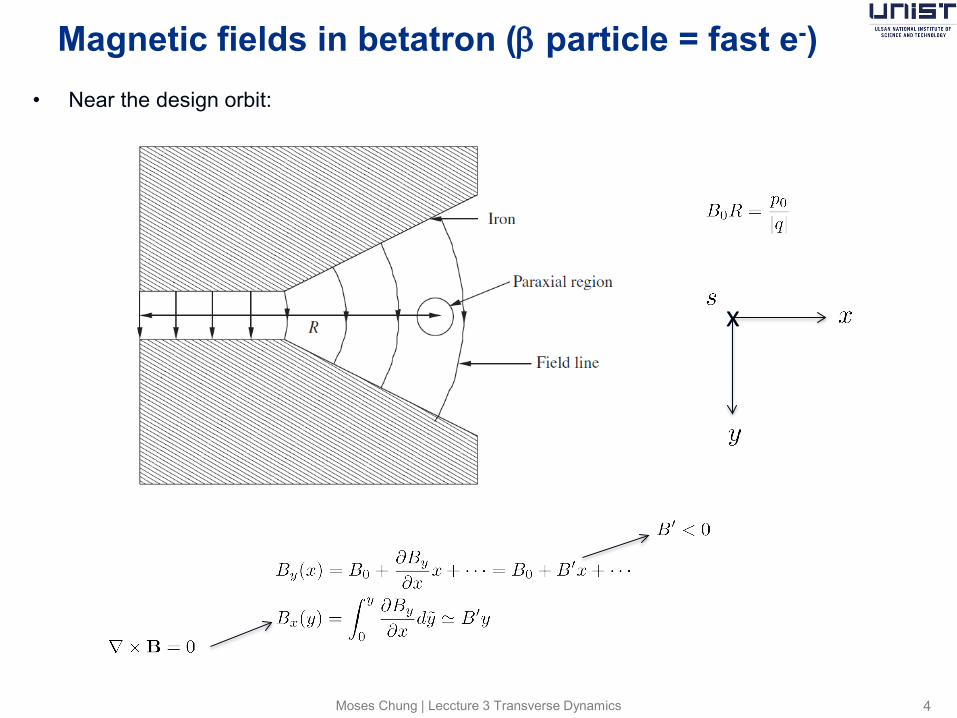
Magnetic fields in betatron (β particle = fast e-)


• Near the design orbit:

x

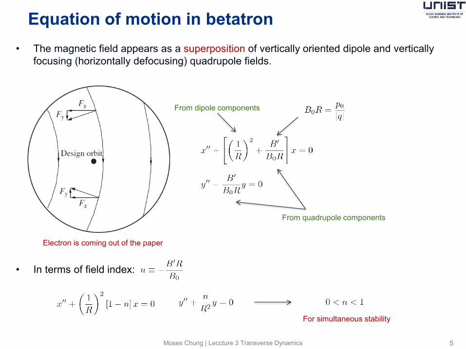
Equation of motion in betatron


• The magnetic field appears as a superposition of vertically oriented dipole and vertically focusing (horizontally defocusing) quadrupole fields.

• In terms of field index:

Electron is coming out of the paper

From quadrupole components

From dipole components

For simultaneous stability

Tunes (denoted by either 𝝂 or Q)


• If we write the equations of motion in terms of azimuthal angle 𝜃 = 𝑠/𝑅:

• The phase changes (or phase advances) per one period (for circular machine considered here, one revolution, 2π) are

• The number of oscillations in the horizontal (x) and vertical (y) dimensions per one period (for circular machine considered here, one revolution, 2π) are called tunes:

• Restriction on tunes for betatron (weak focusing): • Scaling of the maximum offset size of the beam scales with the radius of curvature

We need to make tune very large: Strong focusing


Sec. 3.2

Matrix Analysis of Periodic Focusing System

Periodic focusing


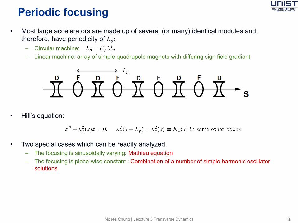
• Most large accelerators are made up of several (or many) identical modules and, therefore, have periodicity of 𝐿𝑝:

– Circular machine: – Linear machine: array of simple quadrupole magnets with differing sign field gradient

• Hill’s equation:

• Two special cases which can be readily analyzed. – The focusing is sinusoidally varying: Mathieu equation – The focusing is piece-wise constant : Combination of a number of simple harmonic oscillator

solutions

Matrix formalism


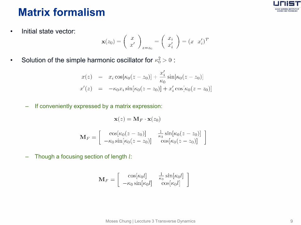
• Initial state vector:

• Solution of the simple harmonic oscillator for :

– If conveniently expressed by a matrix expression:

– Though a focusing section of length 𝑙:

Matrix formalism (cont’d)


• Solution of the simple harmonic oscillator for :

– If conveniently expressed by a matrix expression:

• Limiting cases: – Force-free drift:

– Thin-lens limit:

Focal length

The change in position x is negligible and only the angle x’ is transformed

The position x changes while the angle x’ does not

Length of drift space

[Example 1] Doublet


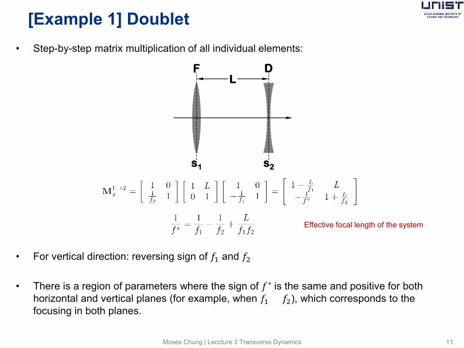
• Step-by-step matrix multiplication of all individual elements:

• For vertical direction: reversing sign of 𝑓1 and 𝑓2

• There is a region of parameters where the sign of 𝑓∗ is the same and positive for both horizontal and vertical planes (for example, when 𝑓1 = 𝑓2), which corresponds to the focusing in both planes.

Effective focal length of the system

[Example 2] FODO lattice


• Focus(F)-Drift(O)-Defocus(D)-Drift(O) lattice:

• Note that the matrix product given in Eq. (3.20) is written in reverse order from that in which the component matrices are physically encountered in the beam line. Confusion on the ordering of matrices is the most common mistake made in the matrix analysis of beam dynamics!

What about y direction ?

[Note] General properties of linear transformation


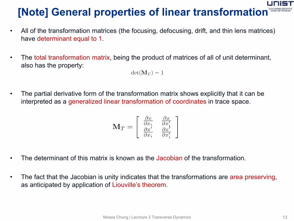
• All of the transformation matrices (the focusing, defocusing, drift, and thin lens matrices) have determinant equal to 1.

• The total transformation matrix, being the product of matrices of all of unit determinant, also has the property:

• The partial derivative form of the transformation matrix shows explicitly that it can be interpreted as a generalized linear transformation of coordinates in trace space.

• The determinant of this matrix is known as the Jacobian of the transformation.

• The fact that the Jacobian is unity indicates that the transformations are area preserving, as anticipated by application of Liouville’s theorem.

Stability analysis


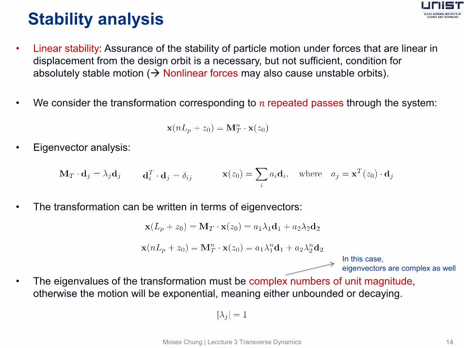
• Linear stability: Assurance of the stability of particle motion under forces that are linear in displacement from the design orbit is a necessary, but not sufficient, condition for absolutely stable motion ( Nonlinear forces may also cause unstable orbits).

• We consider the transformation corresponding to 𝑛 repeated passes through the system:

• Eigenvector analysis:

• The transformation can be written in terms of eigenvectors:

• The eigenvalues of the transformation must be complex numbers of unit magnitude, otherwise the motion will be exponential, meaning either unbounded or decaying.

In this case, eigenvectors are complex as well

Eigenvalue problem


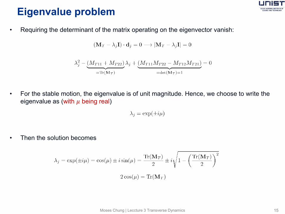
• Requiring the determinant of the matrix operating on the eigenvector vanish:

• For the stable motion, the eigenvalue is of unit magnitude. Hence, we choose to write the eigenvalue as (with 𝜇 being real)

• Then the solution becomes

Stability condition


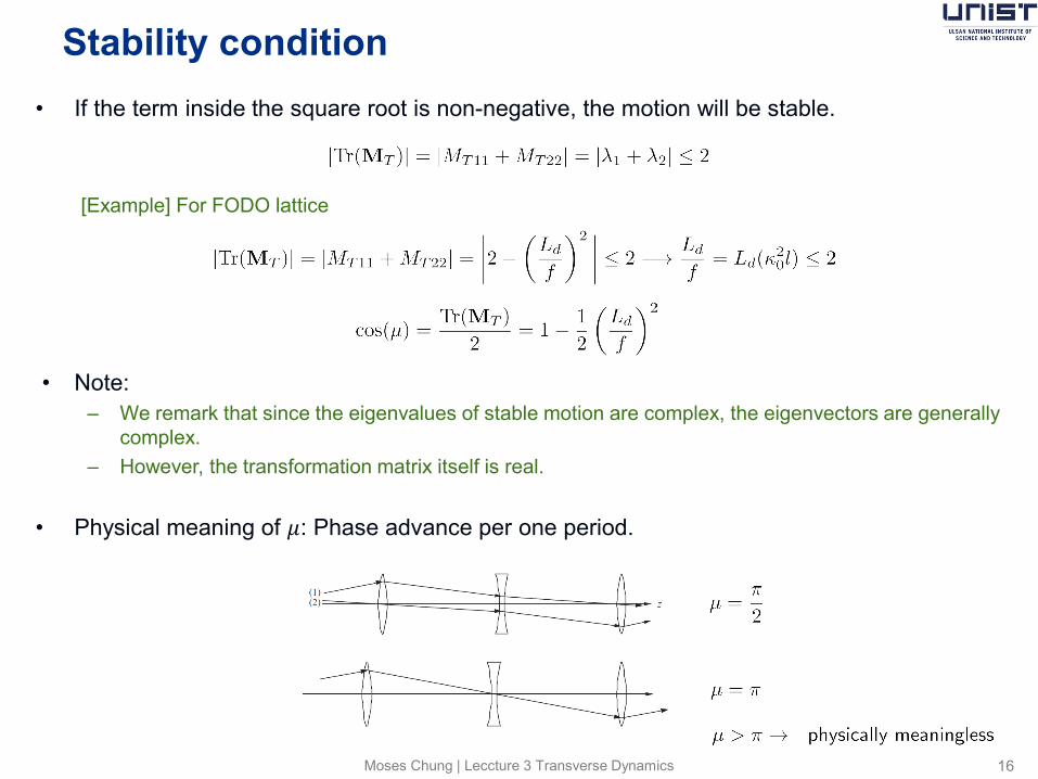
• If the term inside the square root is non-negative, the motion will be stable.

[Example] For FODO lattice

• Note: – We remark that since the eigenvalues of stable motion are complex, the eigenvectors are generally

complex. – However, the transformation matrix itself is real.

• Physical meaning of 𝜇: Phase advance per one period.

Parametrization of the transformation matrix


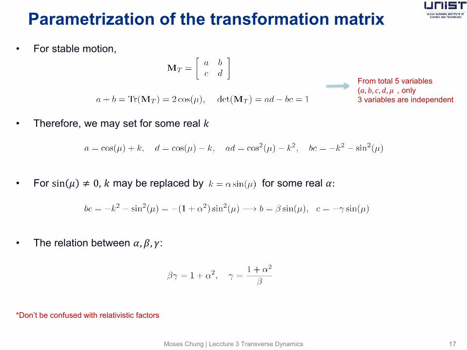
• For stable motion,

• Therefore, we may set for some real 𝑘

• For sin 𝜇 ≠ 0, 𝑘 may be replaced by for some real 𝛼:

• The relation between 𝛼,𝛽, 𝛾:

*Don’t be confused with relativistic factors

From total 5 variables (𝑎, 𝑏, 𝑐, 𝑑, 𝜇), only 3 variables are independent



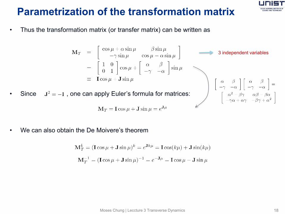
• Thus the transformation matrix (or transfer matrix) can be written as

• Since , one can apply Euler’s formula for matrices:

• We can also obtain the De Moivere’s theorem

3 independent variables



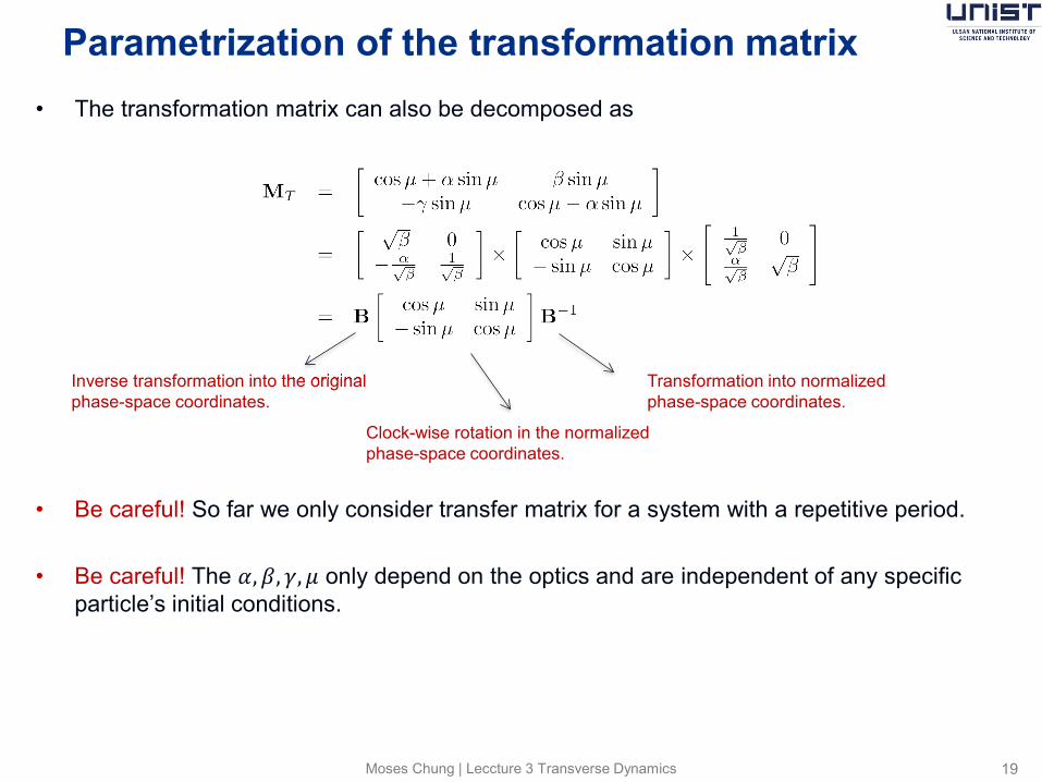
• The transformation matrix can also be decomposed as

• Be careful! So far we only consider transfer matrix for a system with a repetitive period.

• Be careful! The 𝛼,𝛽, 𝛾,𝜇 only depend on the optics and are independent of any specific particle’s initial conditions.

Transformation into normalized phase-space coordinates.

Inverse transformation into the original phase-space coordinates.

Clock-wise rotation in the normalized phase-space coordinates.


Sec. 3.3

Visualization of Motion in Periodic Focusing System

Typical trajectory


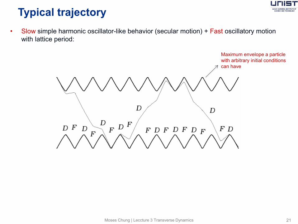
• Slow simple harmonic oscillator-like behavior (secular motion) + Fast oscillatory motion with lattice period:

Maximum envelope a particle with arbitrary initial conditions can have

Trace space plot in periodic focusing system


The fast motion, despite its small spatial amplitude, will also be seen to have relatively large angles associated with it.

The fast errors in the trajectory have large angular oscillations, and the trace space plot fills in a distorted annular region, yielding unclear information about the nature of the trajectory

For simple harmonic oscillator case

Poincare plot (Stroboscopic plot)


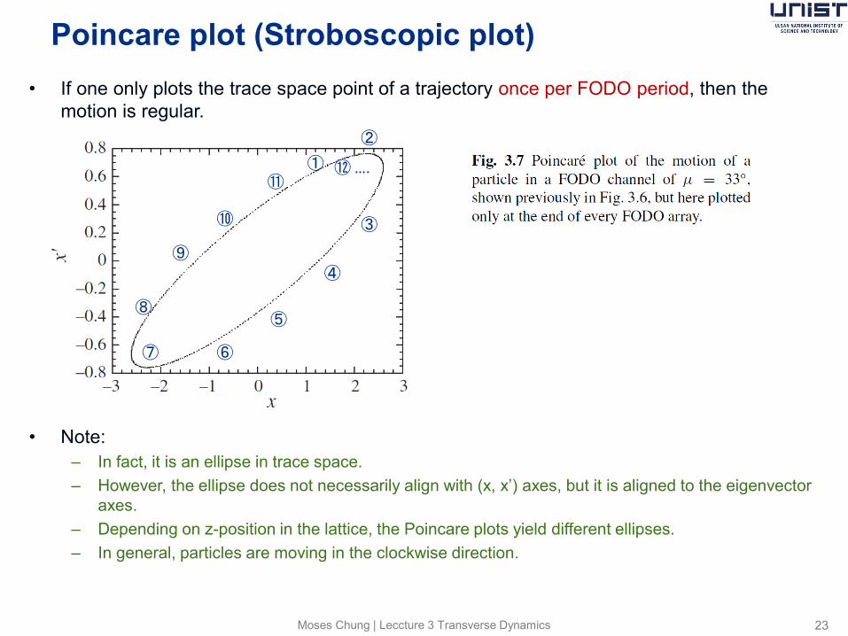
• If one only plots the trace space point of a trajectory once per FODO period, then the motion is regular.

• Note: – In fact, it is an ellipse in trace space. – However, the ellipse does not necessarily align with (x, x’) axes, but it is aligned to the eigenvector

axes. – Depending on z-position in the lattice, the Poincare plots yield different ellipses. – In general, particles are moving in the clockwise direction.

⑦

① ②

③

④

⑤

⑥

⑪

⑩

⑨

⑧

⑫ ….

Smooth approximation


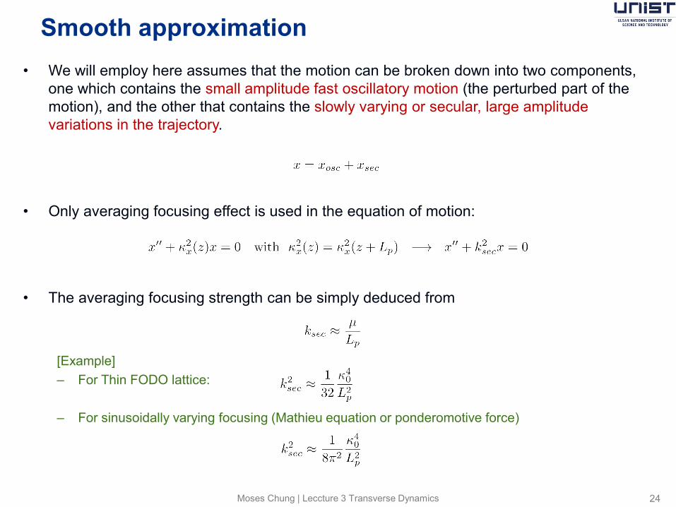
• We will employ here assumes that the motion can be broken down into two components, one which contains the small amplitude fast oscillatory motion (the perturbed part of the motion), and the other that contains the slowly varying or secular, large amplitude variations in the trajectory.

• Only averaging focusing effect is used in the equation of motion:

• The averaging focusing strength can be simply deduced from

[Example] – For Thin FODO lattice: – For sinusoidally varying focusing (Mathieu equation or ponderomotive force)


Secs. 2.4.1/2.4.2/2.4.6 of UP-ALP

Analytic approach for Hill’s equation

2.4.1 Pseudo-harmonic oscillations


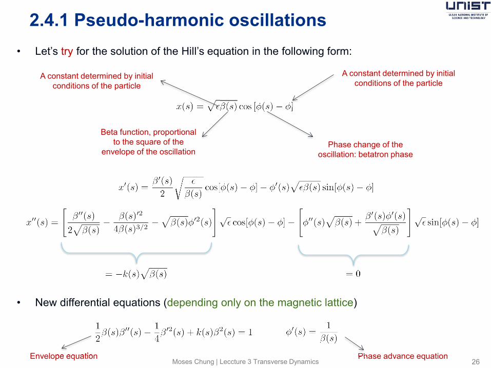
• Let’s try for the solution of the Hill’s equation in the following form:

• New differential equations (depending only on the magnetic lattice)

Beta function, proportional to the square of the

envelope of the oscillation

A constant determined by initial conditions of the particle

Phase change of the oscillation: betatron phase

A constant determined by initial conditions of the particle

Envelope equation Phase advance equation

2.4.2 Principal trajectory


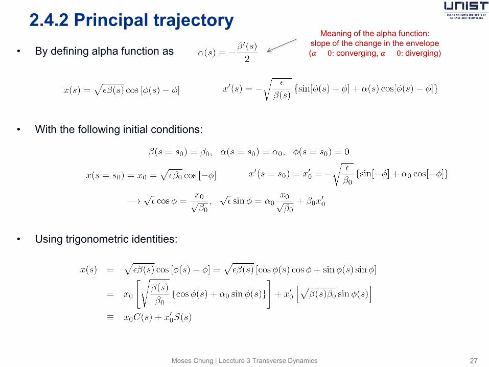
• By defining alpha function as

• With the following initial conditions:

• Using trigonometric identities:

Meaning of the alpha function: slope of the change in the envelope (𝛼 > 0: converging, 𝛼 < 0: diverging)

2.4.2 Principal trajectory (cont’d)


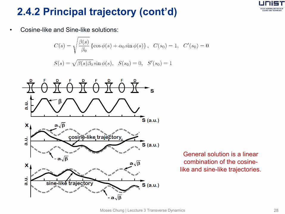
• Cosine-like and Sine-like solutions:

General solution is a linear combination of the cosine-

like and sine-like trajectories.

2.4.7 Connection with matrix formalism


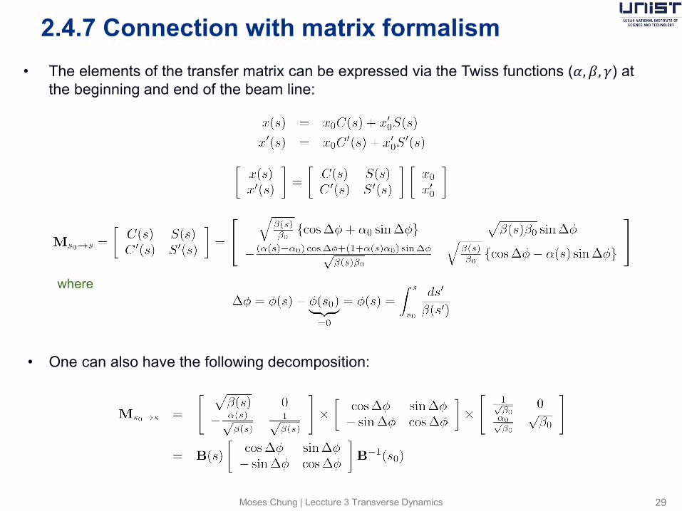
• The elements of the transfer matrix can be expressed via the Twiss functions (𝛼,𝛽, 𝛾) at the beginning and end of the beam line:

where

• One can also have the following decomposition:

2.4.7 Connection with matrix formalism


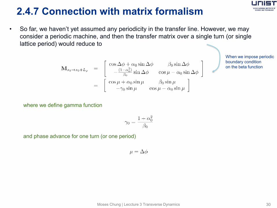
• So far, we haven’t yet assumed any periodicity in the transfer line. However, we may consider a periodic machine, and then the transfer matrix over a single turn (or single lattice period) would reduce to

where we define gamma function and phase advance for one turn (or one period)

When we impose periodic boundary condition on the beta function

2.5.1 Courant-Snyder invariant


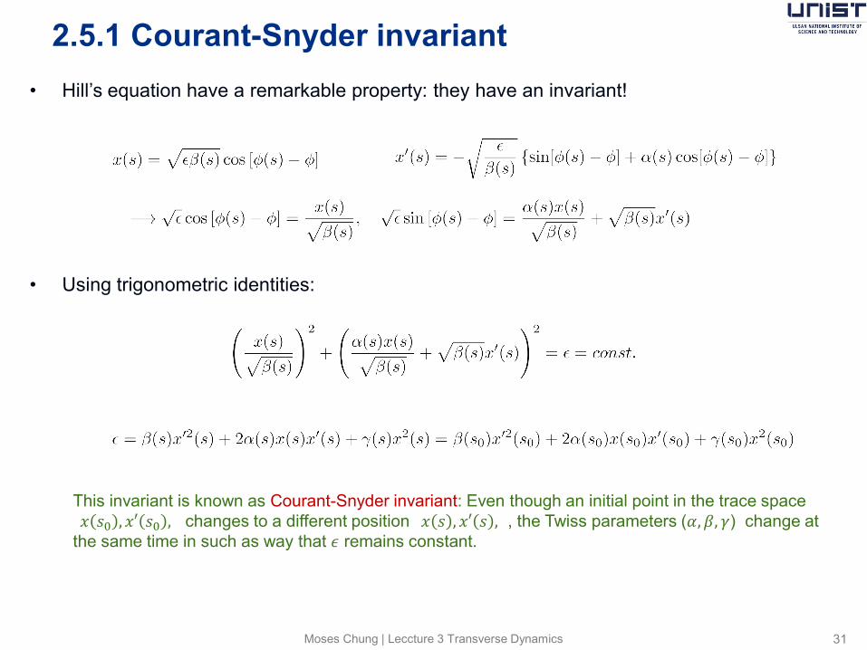
• Hill’s equation have a remarkable property: they have an invariant!

• Using trigonometric identities:

This invariant is known as Courant-Snyder invariant: Even though an initial point in the trace space (𝑥 𝑠0 ,𝑥′ 𝑠0 , ) changes to a different position (𝑥 𝑠 , 𝑥′ 𝑠 , ), the Twiss parameters (𝛼,𝛽, 𝛾) change at the same time in such as way that 𝜖 remains constant.

2.5.1 Phase space (or trace space) ellipse


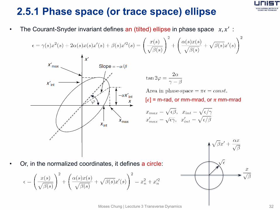
• The Courant-Snyder invariant defines an (tilted) ellipse in phase space (𝑥, 𝑥′):

• Or, in the normalized coordinates, it defines a circle:

[𝜖] = m-rad, or mm-mrad, or 𝜋 mm-mrad

[Example]


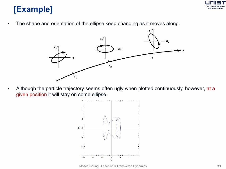
• The shape and orientation of the ellipse keep changing as it moves along.

• Although the particle trajectory seems often ugly when plotted continuously, however, at a

given position it will stay on some ellipse.

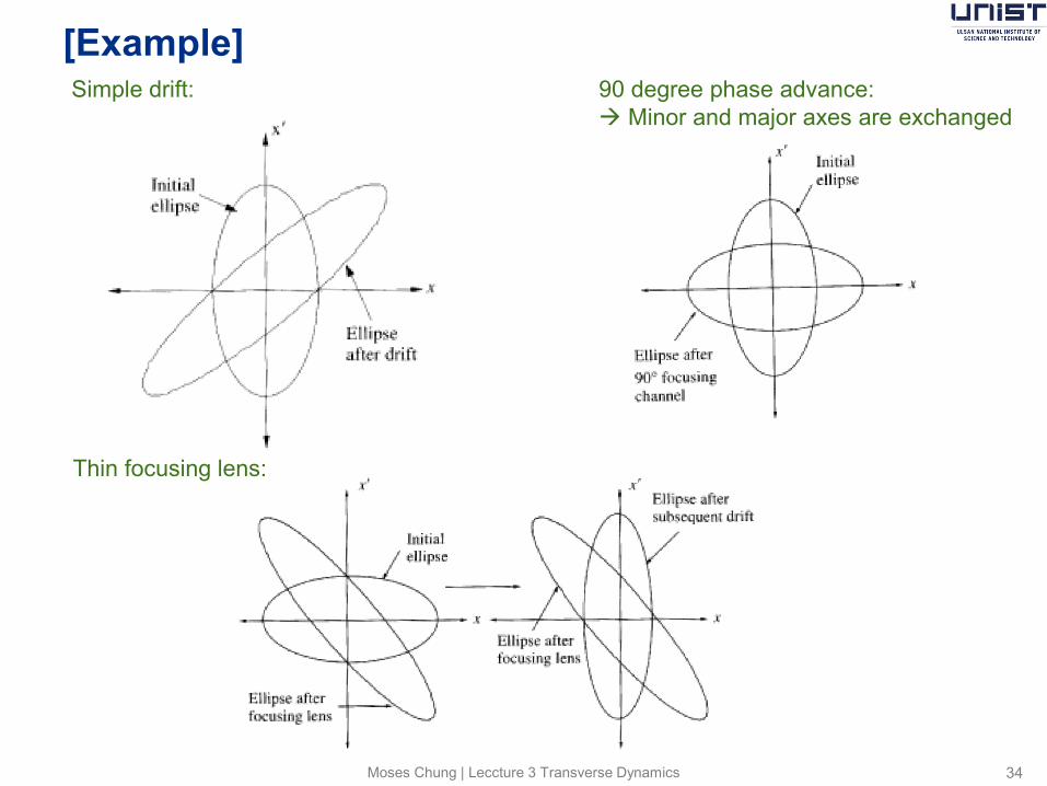
[Example]


Simple drift: 90 degree phase advance: Minor and major axes are exchanged

Thin focusing lens:

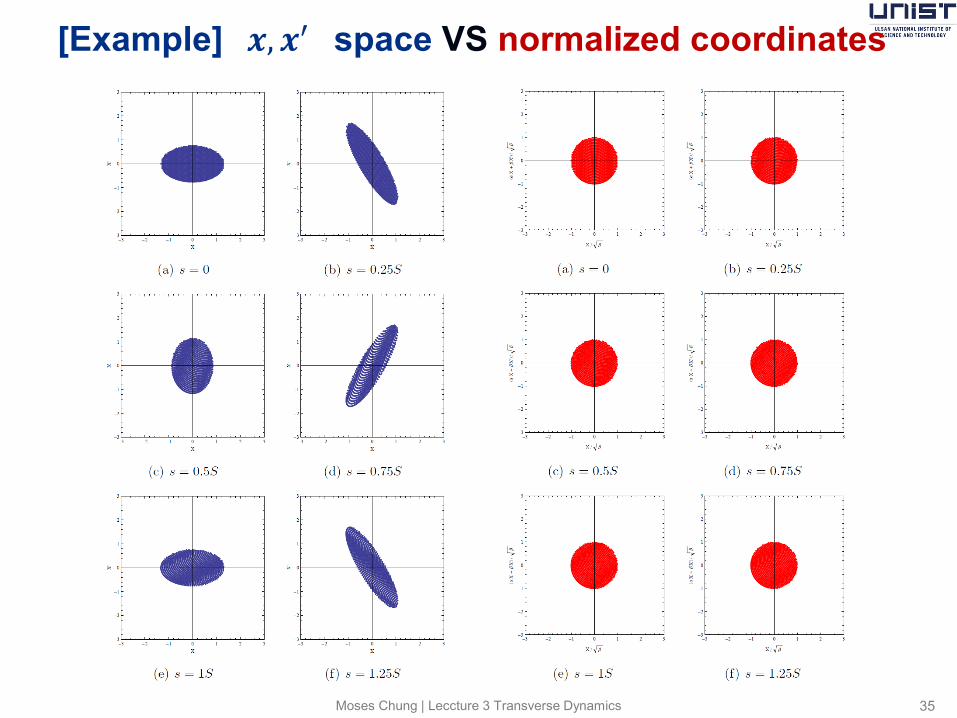
[Example] (𝒙,𝒙′) space VS normalized coordinates


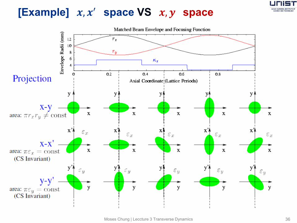
[Example] (𝒙,𝒙′) space VS (𝒙,𝒚) space



Secs. 5.2/5.3/5.4 of FOBP

Beam Distribution and Emittance

Bi-Gaussian distribution


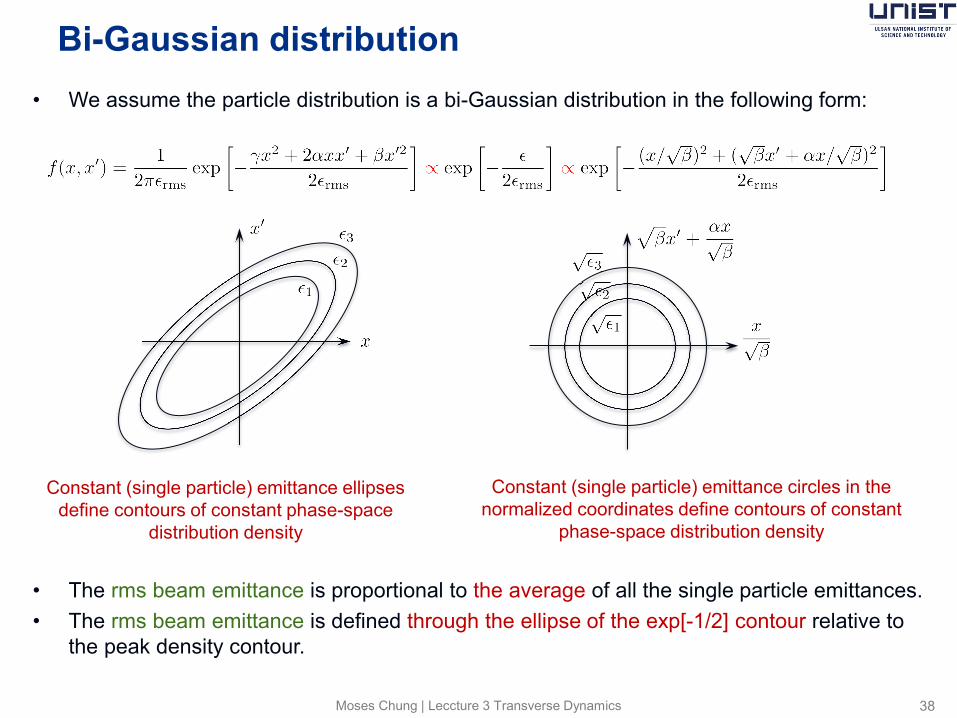
• We assume the particle distribution is a bi-Gaussian distribution in the following form:

• The rms beam emittance is proportional to the average of all the single particle emittances. • The rms beam emittance is defined through the ellipse of the exp[-1/2] contour relative to

the peak density contour.

Constant (single particle) emittance ellipses define contours of constant phase-space

distribution density

Constant (single particle) emittance circles in the normalized coordinates define contours of constant

phase-space distribution density

Normalization of the distribution function


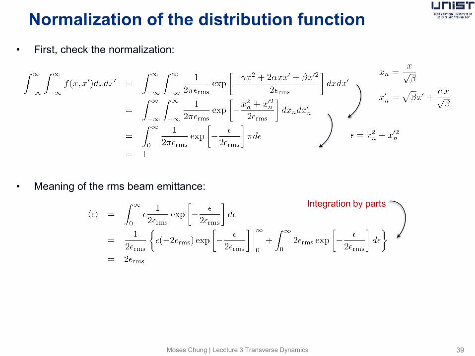
• First, check the normalization:

• Meaning of the rms beam emittance:

Integration by parts

Moments of the distribution function


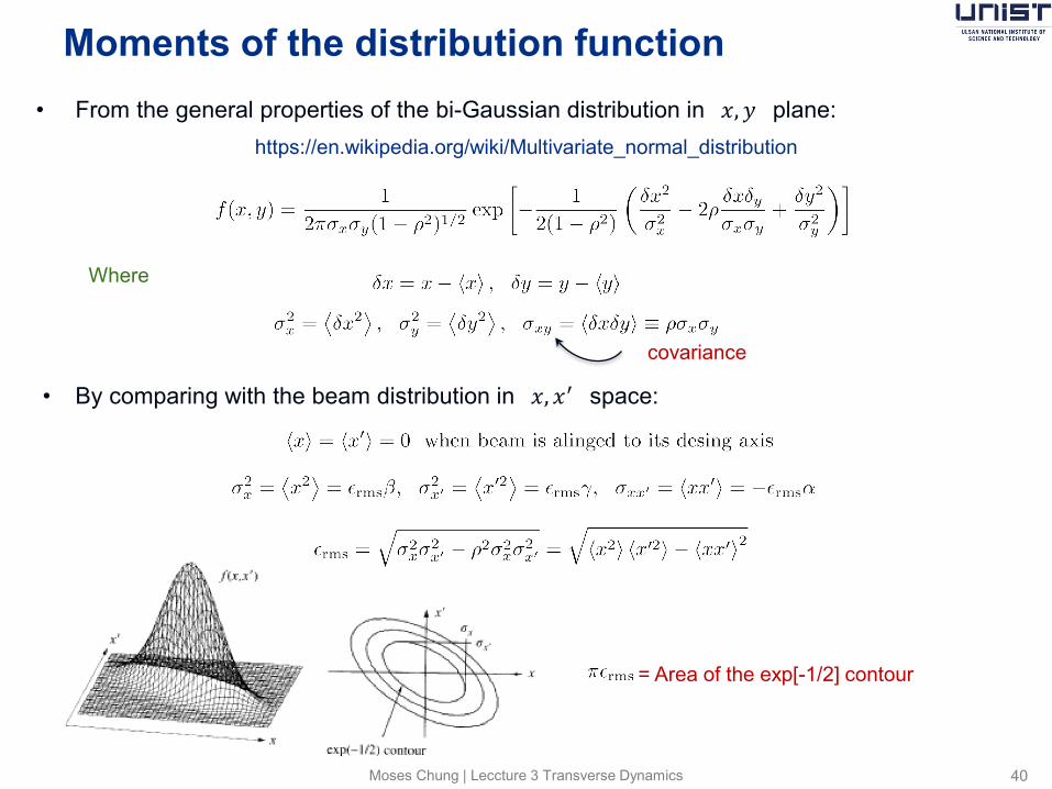
• From the general properties of the bi-Gaussian distribution in (𝑥,𝑦) plane:

Where

• By comparing with the beam distribution in (𝑥, 𝑥′) space:

https://en.wikipedia.org/wiki/Multivariate_normal_distribution

covariance

= Area of the exp[-1/2] contour

Beam matrix


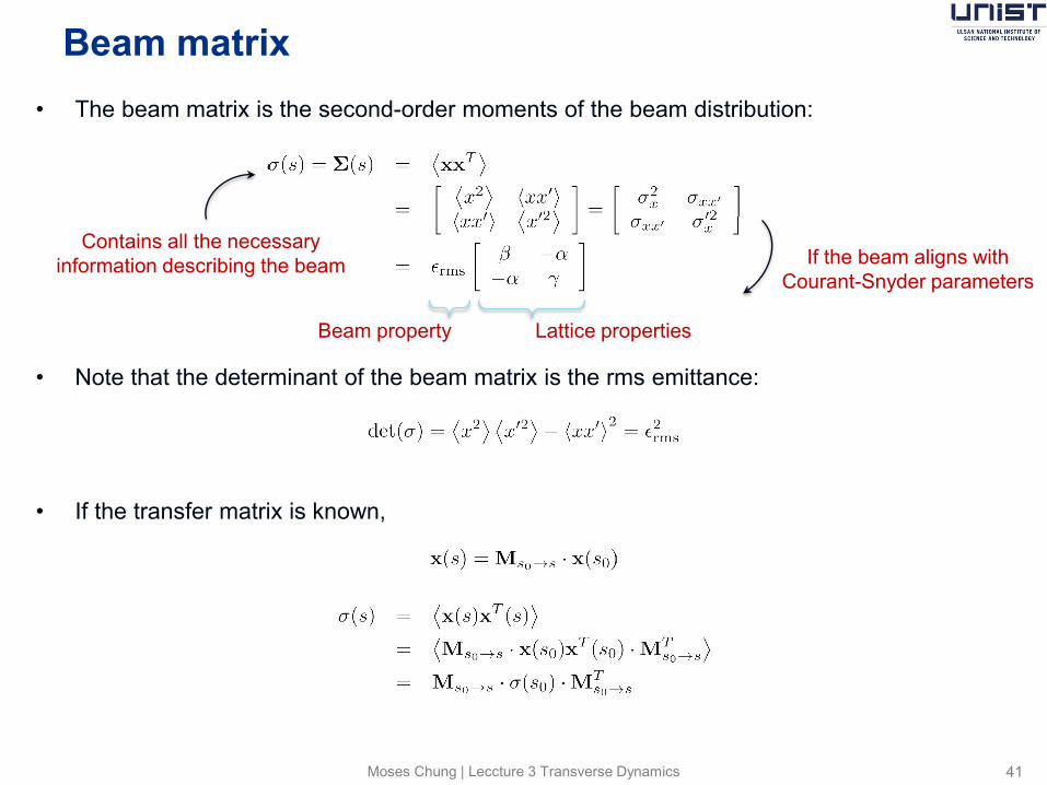
• The beam matrix is the second-order moments of the beam distribution:

• Note that the determinant of the beam matrix is the rms emittance:

• If the transfer matrix is known,

If the beam aligns with Courant-Snyder parameters

Contains all the necessary information describing the beam

Lattice properties Beam property

Fraction of particles enclosed


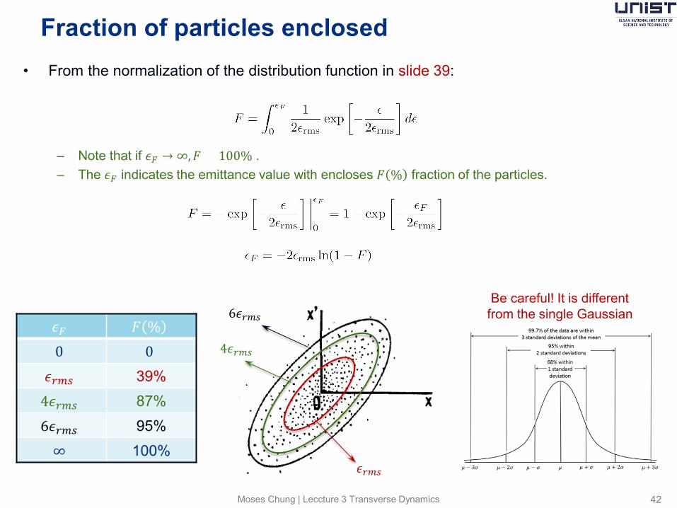
• From the normalization of the distribution function in slide 39:

– Note that if 𝜖𝐹 → ∞,𝐹 = 100% . – The 𝜖𝐹 indicates the emittance value with encloses 𝐹 % fraction of the particles.

𝜖𝐹 𝐹 % 0 0

𝜖𝑟𝑟𝑟 39% 4𝜖𝑟𝑟𝑟 87% 6𝜖𝑟𝑟𝑟 95% ∞ 100%

Be careful! It is different from the single Gaussian 6𝜖𝑟𝑟𝑟

𝜖𝑟𝑟𝑟

4𝜖𝑟𝑟𝑟

If the beam is not in thermal equilibrium:


• We used bi-Gaussian distribution assuming that the beam is in thermal equilibrium:

• Even though the beam distribution function is not exactly in thermal equilibrium, it is often used as a good approximation.

• For example, in the periodic focusing system, the particle motion is always non-equillibirum, however, when plotted in trace space once per period (i.e., in the Poincare plot), we can treat the beam in equilibrium.

• Thermalization is often achieved very slowly, over many revolutions of a circular accelerator, by a combination of damping and heating effects (e.g., radiation emission, intra-beam scattering).

• In fast, transient systems, such as linear accelerators, equilibrating mechanisms (i.e. collisions) are too slow to be relevant, and if equilibria are found, they must be a property of the particle source used (Collective effects may enhance relaxation rate though).

If the focusing force is not linear:


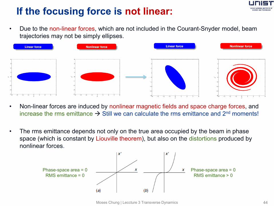
• Due to the non-linear forces, which are not included in the Courant-Snyder model, beam trajectories may not be simply ellipses.

• Non-linear forces are induced by nonlinear magnetic fields and space charge forces, and

increase the rms emittance Still we can calculate the rms emittance and 2nd moments!

• The rms emittance depends not only on the true area occupied by the beam in phase space (which is constant by Liouville theorem), but also on the distortions produced by nonlinear forces.

Phase-space area = 0 RMS emittance = 0

Phase-space area = 0 RMS emittance > 0

If the beam is not matching with the ellipse:


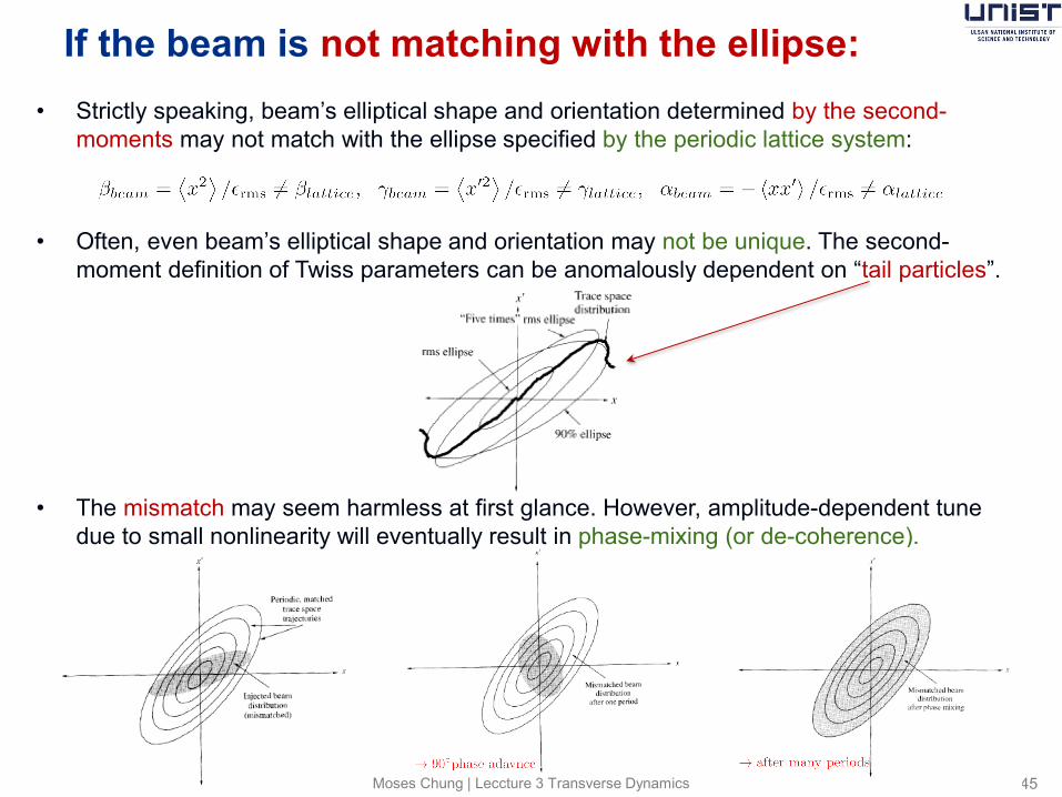
• Strictly speaking, beam’s elliptical shape and orientation determined by the second-moments may not match with the ellipse specified by the periodic lattice system:

• Often, even beam’s elliptical shape and orientation may not be unique. The second-

moment definition of Twiss parameters can be anomalously dependent on “tail particles”.

• The mismatch may seem harmless at first glance. However, amplitude-dependent tune due to small nonlinearity will eventually result in phase-mixing (or de-coherence).


Sec. 2.4.3 of UP-ALP/ Sec. 3.5 of FOBP

Edge Focusing

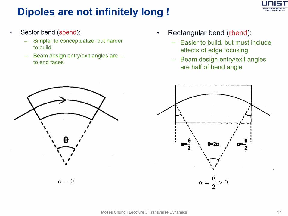
Dipoles are not infinitely long !


• Sector bend (sbend): – Simpler to conceptualize, but harder

to build – Beam design entry/exit angles are ⊥

to end faces

• Rectangular bend (rbend): – Easier to build, but must include

effects of edge focusing – Beam design entry/exit angles

are half of bend angle

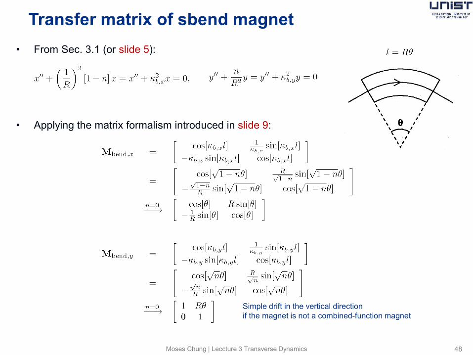
Transfer matrix of sbend magnet


• From Sec. 3.1 (or slide 5):

• Applying the matrix formalism introduced in slide 9:

Simple drift in the vertical direction if the magnet is not a combined-function magnet

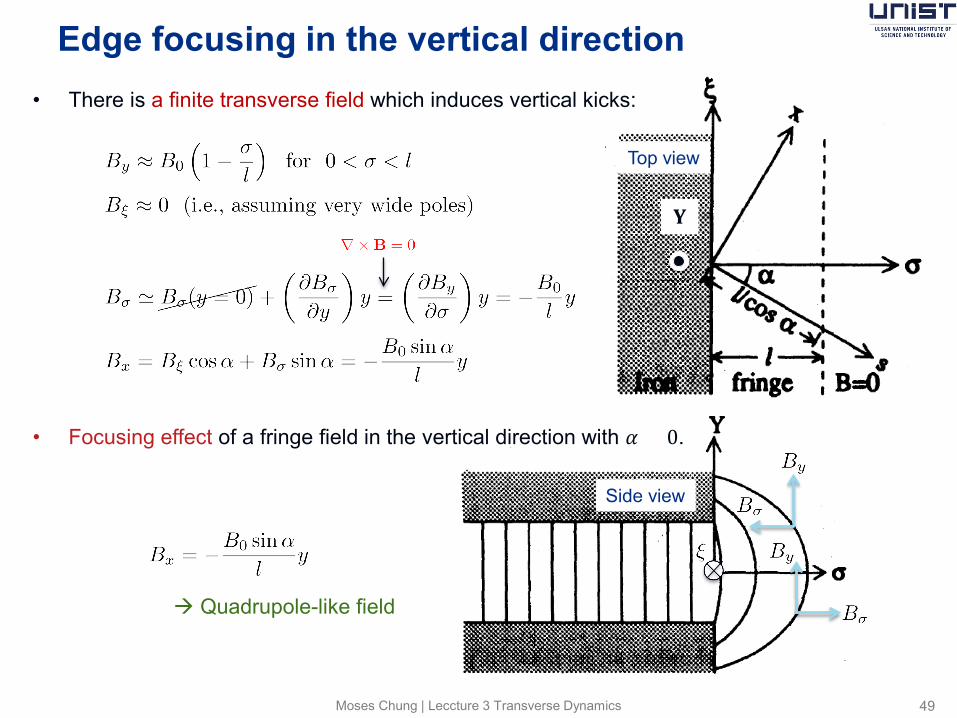
Edge focusing in the vertical direction


• There is a finite transverse field which induces vertical kicks:

• Focusing effect of a fringe field in the vertical direction with 𝛼 > 0.

𝐘

Top view

Side view

Quadrupole-like field

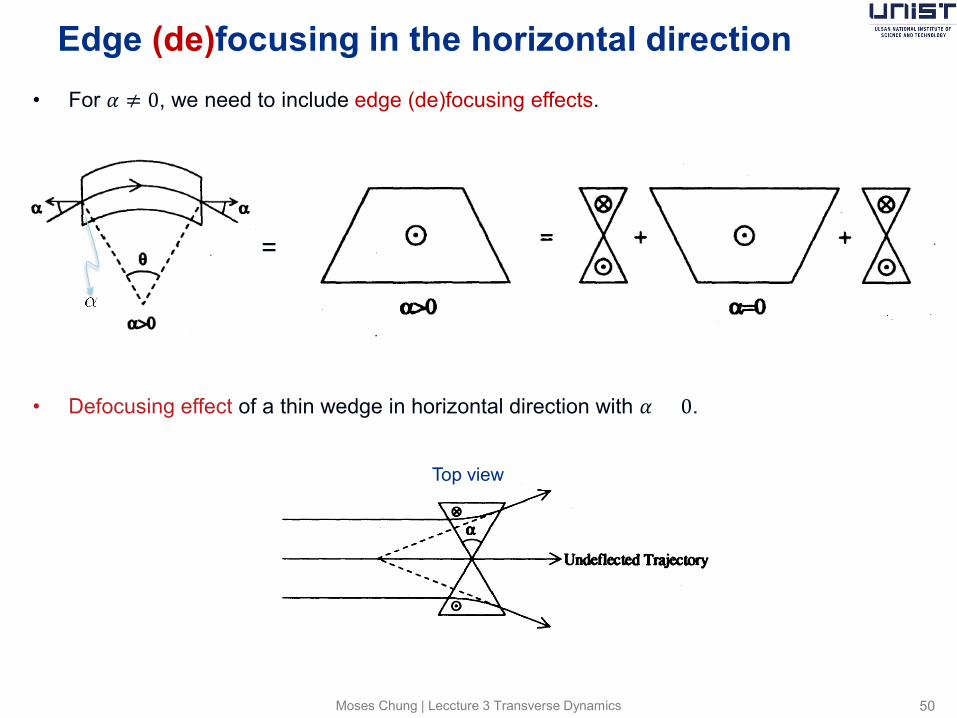
Edge (de)focusing in the horizontal direction


• For 𝛼 ≠ 0, we need to include edge (de)focusing effects.

• Defocusing effect of a thin wedge in horizontal direction with 𝛼 > 0.

=

Top view

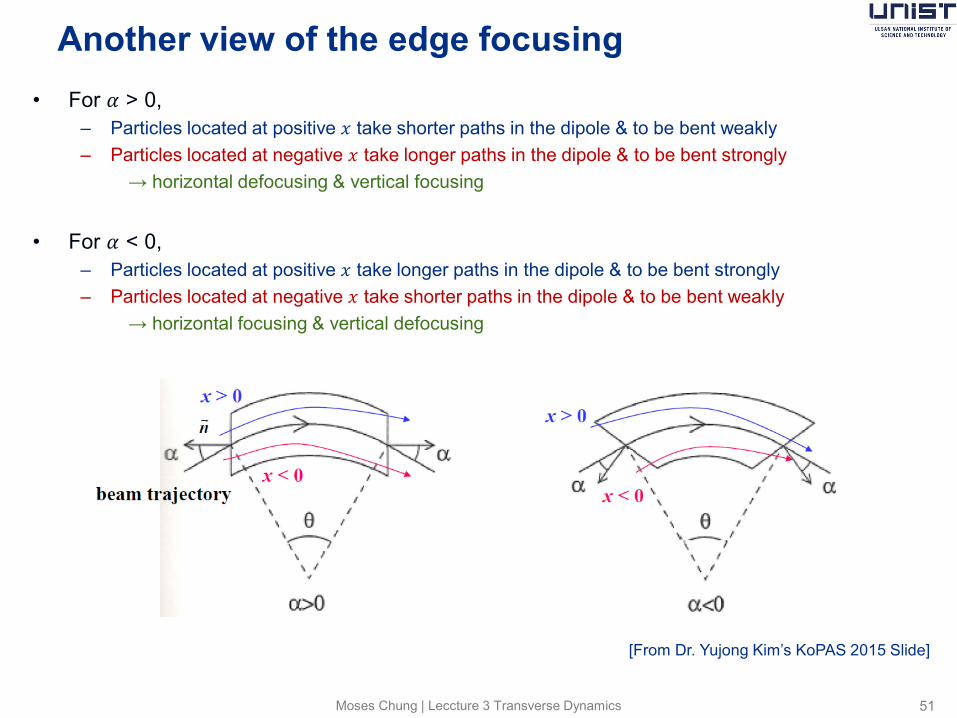
Another view of the edge focusing


• For 𝛼 > 0, – Particles located at positive 𝑥 take shorter paths in the dipole & to be bent weakly – Particles located at negative 𝑥 take longer paths in the dipole & to be bent strongly → horizontal defocusing & vertical focusing

• For 𝛼 < 0,

– Particles located at positive 𝑥 take longer paths in the dipole & to be bent strongly – Particles located at negative 𝑥 take shorter paths in the dipole & to be bent weakly → horizontal focusing & vertical defocusing

[From Dr. Yujong Kim’s KoPAS 2015 Slide]

lecture 3 ‘linear’ transverse...

Documents