1

Lecture 24: Spinodal Decomposition: Part 3: kinetics of the

composition fluctuation

Today’s topics

• Diffusion kinetics of spinodal decomposition in terms of the concentration (composition)

fluctuation as a function of time: 0( , ) ( ,0) exp[ ( ) ] cosmc x t c A R t xβ β β− = ⋅ ⋅ , where

0

22 2

20

( ) [ 2 ]cM gR KN c

β β β∂

= − ⋅ ⋅ +∂

• Learn how to derive above equation from the Fick’s second law, for which how to deduce the

term gc∂

∂is critical,

0

2 2

02 2( ) 2cg g d cc c Kc c dx∂ ∂

= − −∂ ∂

.

• Understand the critical wavelength λc (or wave number βc) for the composition fluctuation: for

Cβ β< (or Cλ λ> ), then ( ) 0R β > , the composition fluctuations (amplitude) will grow ---

thermodynamically favorable. • Understand the maximal wavelength λm (or wave number βm), at which the composition

fluctuations (amplitude) will grow the fastest: when mβ β<< (or mλ λ>> ), the growth

becomes diffusion limited.

Phase diagram and free energy plot of Spinodal Decomposition

As a special case of phase transformation, spinodal decomposition can be illustrated on a phase diagram exhibiting a miscibility gap (see the diagram below). Thus, phase separation occurs whenever a material transitions into the unstable region of the phase diagram. The boundary of the unstable region, sometimes referred to as the binodal or coexistence curve, is found by performing a common tangent construction of the free-energy diagram. Inside the binodal is a region called the spinodal, which is found by determining where the curvature of the free-energy curve is negative. The binodal and spinodal meet at the critical point. It is when a material is moved into the spinodal region of the phase diagram that spinodal decomposition can occur. If an alloy with composition of X0 is solution treated at a high temperature T1, and then quenched (rapidly cooled) to a lower temperature T2, the composition will initially be the same everywhere and its free energy will be G0 on the G curve in the following diagram. However, the alloy will be immediately unstable, because small fluctuation in composition that produces A-rich and B-rich regions will cause the total free energy to decrease. Therefore, “up-hill” diffusion (as shown) takes place until the equilibrium

2

compositions X1 and X2 are reached. How such small composition fluctuation leads to the spinodal phase separation is today’s and next two lectures’ topics.

The free energy curve is plotted as a function of composition for the phase separation temperature T2. Equilibrium phase compositions are those corresponding to the free energy minima. Regions of negative curvature (d2G/dc2 < 0 ) lie within the inflection points of the curve (d2G/dc2 = 0 ) which are called the spinodes (as marked as S1 and S2 in the diagram above). For compositions within the spinodal, a homogeneous solution is unstable against microscopic fluctuations in density or composition, and there is no thermodynamic barrier to the growth of a new phase, i.e., the phase transformation is solely diffusion controlled.

In last two lectures (#22, 23): For a homogeneous solid solution of composition C0, when a composition perturbation (or fluctuation) is created such that the composition is a function of position (although the average composition is still c0), the spinodal decomposition will initiated. The composition fluctuation can be described as

02( ) cos( ) cosm mc x c A x A xπ

βλ

− = =

3

where Am = amplitude, and 2π

βλ

= = wave number

Let concentration (molar fraction) of B atom is c, the concentration of A atom is (1-c), Then the interdiffusion coefficient can be expressed as:

D! = c(1− c)N0

{cMA + (1− c)MB}∂2g∂c2

(N0 is the Avogadro constant, kB is the Boltzmann constant.)

Where AA

B

D Mk T

= and BB

B

D Mk T

= , MA and MB are mobilities of A and B, respectively.

Defining [ (1 ) ] (1 )A BM cM c M c c= + − ⋅ ⋅ −

Then, D! = MN0

⋅∂2g∂c2

(Inside the spinodal, ∞D < 0.)

Today’s Lecture: Fick’s first law gives.

J = −D! ⋅ ∂c∂x

= −MN0

⋅∂2g∂c2

⋅∂c∂x

Rewrite the above as

J = −D! ⋅ ∂c∂x

= −MN0

⋅∂∂c(∂g∂c) ⋅ ∂c∂x

0

( )M gN x c

∂ ∂= − ⋅ ⋅

∂ ∂

Then, Fick’s second law becomes

0

[ ( )]c J M gt x x N x c∂ ∂ ∂ ∂ ∂

= − = ⋅ ⋅∂ ∂ ∂ ∂ ∂

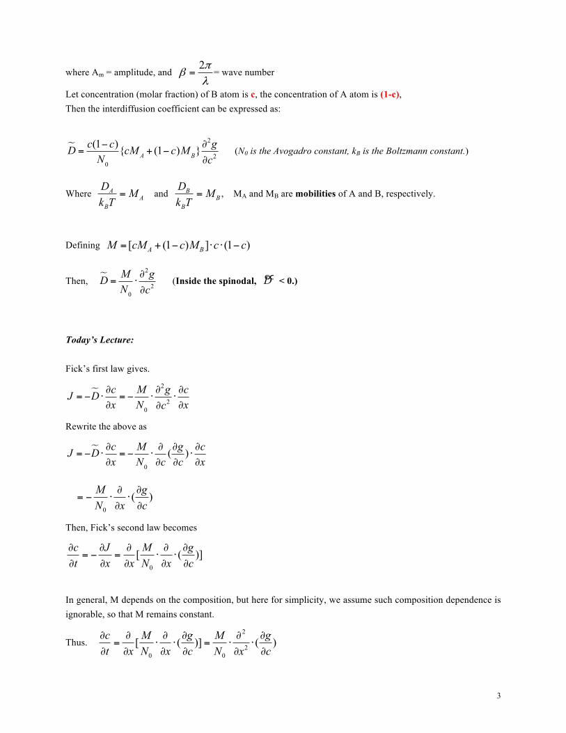
In general, M depends on the composition, but here for simplicity, we assume such composition dependence is ignorable, so that M remains constant.

Thus. 2

20 0

[ ( )] ( )c M g M gt x N x c N x c∂ ∂ ∂ ∂ ∂ ∂

= ⋅ ⋅ = ⋅ ⋅∂ ∂ ∂ ∂ ∂ ∂

4

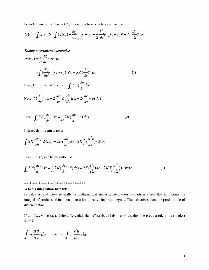
From Lecture 23, we know G(c) per unit volume can be expressed as

0

0

22 2

0 0 02

1( ) ( ) [ ( ) ( ) ( ) ( ) ]2 cx x

c

g g dcG c g c dx g c c c c c K dxc c dx∂ ∂

= = + − + − +∂ ∂∫ ∫

Taking a variational derivative

( )x

gG c c dxc

δ δ∂

= ⋅ ⋅∂∫

0

22

02[ ( ) ( ) ]cx

g dcc c c K dxc dx

δ δ∂

= − ⋅ +∂∫ (1)

Now, let us evaluate the term 2( )x

dcK dxdx

δ∫

Note δ(dcdx)2dx = 2 dc

dx⋅δ(dcdx)dx = 2(dc

dx) ⋅δ(dc)

Thus, 2( ) 2 ( ) ( )x x

dc dcK dx K dcdx dx

δ δ= ⋅∫ ∫ (2)

Integration by parts gives

2

22 ( ) ( ) 2 ( ) 2 ( )x x

dc dc d cK dc K dc K dx cdx dx dx

δ δ⋅ = − ⋅∫ ∫

Then, Eq. (2) can be re-written as:

22

2( ) 2 ( ) ( ) 2 ( ) 2 ( )x x x

dc dc dc d cK dx K dc K dc K dx cdx dx dx dx

δ δ δ= ⋅ = − ⋅∫ ∫ ∫ (3)

********************************** What is integration by parts: In calculus, and more generally in mathematical analysis, integration by parts is a rule that transforms the integral of products of functions into other (ideally simpler) integrals. The rule arises from the product rule of differentiation. If u = f(x), v = g(x), and the differentials du = f '(x) dx and dv = g'(x) dx, then the product rule in its simplest form is:

5

*********************************

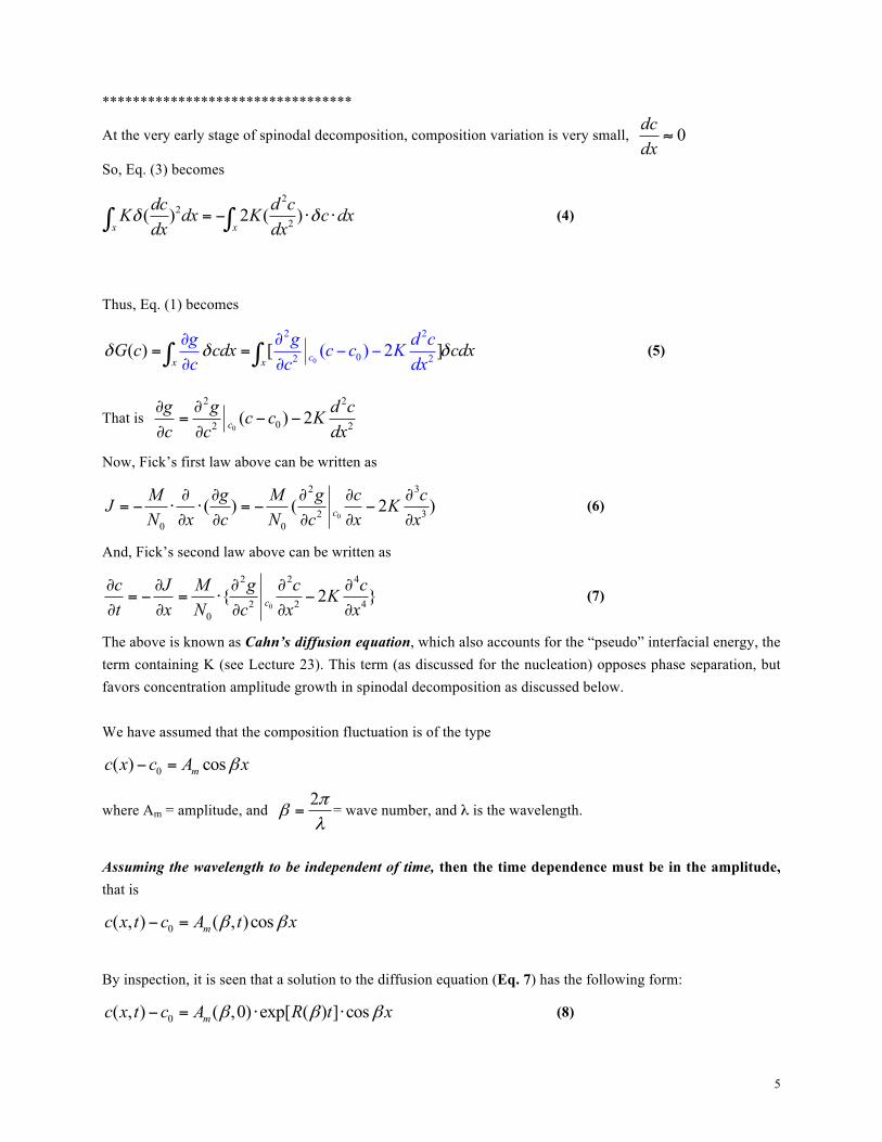
At the very early stage of spinodal decomposition, composition variation is very small, 0dcdx

≈

So, Eq. (3) becomes

22

2( ) 2 ( )x x

dc d cK dx K c dxdx dx

δ δ= − ⋅ ⋅∫ ∫ (4)

Thus, Eq. (1) becomes

0

2 2

02 2( ) 2( ) [ ]cx x

g g d cc cG c cdx cKd

dc c

xx

δ δ δ∂ ∂

− −∂ ∂

= =∫ ∫ (5)

That is 0

2 2

02 2( ) 2cg g d cc c Kc c dx∂ ∂

= − −∂ ∂

Now, Fick’s first law above can be written as

0

2 3

2 30 0

( ) ( 2 )cM g M g c cJ KN x c N c x x

∂ ∂ ∂ ∂ ∂= − ⋅ ⋅ = − −

∂ ∂ ∂ ∂ ∂ (6)

And, Fick’s second law above can be written as

0

2 2 4

2 2 40

{ 2 }cc J M g c cKt x N c x x∂ ∂ ∂ ∂ ∂

= − = ⋅ −∂ ∂ ∂ ∂ ∂

(7)

The above is known as Cahn’s diffusion equation, which also accounts for the “pseudo” interfacial energy, the term containing K (see Lecture 23). This term (as discussed for the nucleation) opposes phase separation, but favors concentration amplitude growth in spinodal decomposition as discussed below. We have assumed that the composition fluctuation is of the type

0( ) cosmc x c A xβ− =

where Am = amplitude, and 2π

βλ

= = wave number, and λ is the wavelength.

Assuming the wavelength to be independent of time, then the time dependence must be in the amplitude, that is

0( , ) ( , )cosmc x t c A t xβ β− =

By inspection, it is seen that a solution to the diffusion equation (Eq. 7) has the following form:

0( , ) ( ,0) exp[ ( ) ] cosmc x t c A R t xβ β β− = ⋅ ⋅ (8)

6

where 0

22 2

20

( ) [ 2 ]cM gR KN c

β β β∂

= − ⋅ ⋅ +∂

(9)

( )R β is termed amplification factor. As long as the term inside the parentheses is negative (note:

0

2

2 cgc∂

∂<0 in the spinodal), ( ) 0R β > , and the amplitude will grow (see the diagram below) --- the critical β

is thus defined as: β c=0

21/ 2

2( / 2 )cg Kc∂

−∂

, and λ c=2π /β , or 0

21/ 2

2 2

2 1[ ( )]8c

c c

gK c

πλ

β π−∂

= = −∂

i.e., the largest β (or smallest λ) possible for the composition (c0) at a temperature to vary. ---this is consistent with what we learned in Lecture 23, where

To have 0

2 22

2{ 2 } 04m

c

A gg Kc

β∂

Δ = + ≤∂

, i.e., to assure spontaneous process,

We deduced the same β c=0

21/ 2

2( / 2 )cg Kc∂

−∂

, and 0

21/ 2

2 2

2 1[ ( )]8c

c c

gK c

πλ

β π−∂

= = −∂

Clearly, inside the spinodal,

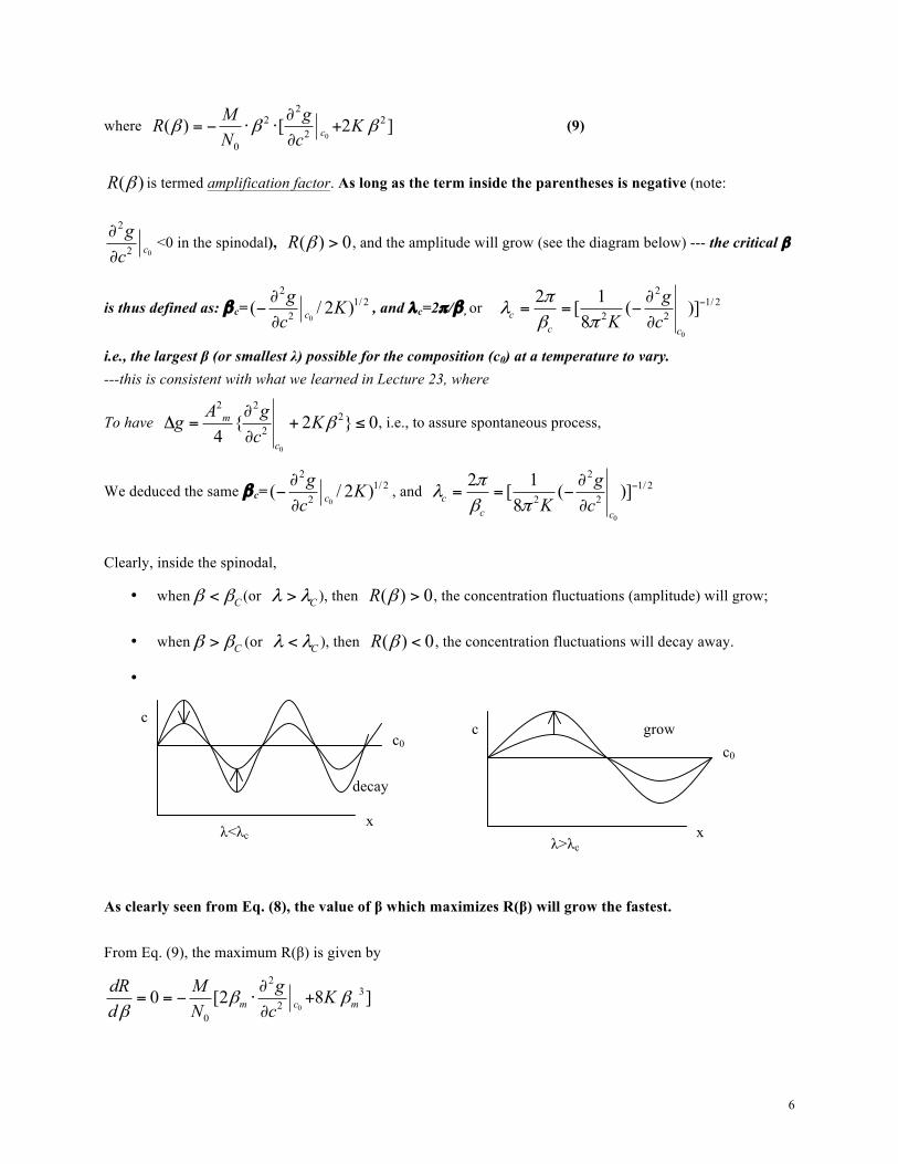
• when Cβ β< (or Cλ λ> ), then ( ) 0R β > , the concentration fluctuations (amplitude) will grow;

• when Cβ β> (or Cλ λ< ), then ( ) 0R β < , the concentration fluctuations will decay away.

•

As clearly seen from Eq. (8), the value of β which maximizes R(β) will grow the fastest. From Eq. (9), the maximum R(β) is given by

0

23

20

0 [2 8 ]m c mdR M g Kd N c

β ββ

∂= = − ⋅ +

∂

c c0

x λ<λc

decay

c c0

x λ>λc

grow

7

so, 0

2

2 14 2

c

m c

gcK

β β

∂−∂= =

or, 2m cλ λ=

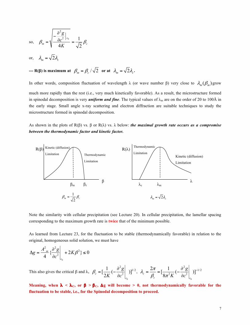
--- R(β) is maximum at / 2m cβ β= or at 2m cλ λ= .

In other words, composition fluctuation of wavelength λ (or wave number β) very close to ( )m mλ β grow

much more rapidly than the rest (i.e., very much kinetically favorable). As a result, the microstructure formed in spinodal decomposition is very uniform and fine. The typical values of λm are on the order of 20 to 100Å in the early stage. Small angle x-ray scattering and electron diffraction are suitable techniques to study the microstructure formed in spinodal decomposition. As shown in the plots of R(β) vs. β or R(λ) vs. λ below: the maximal growth rate occurs as a compromise between the thermodynamic factor and kinetic factor.

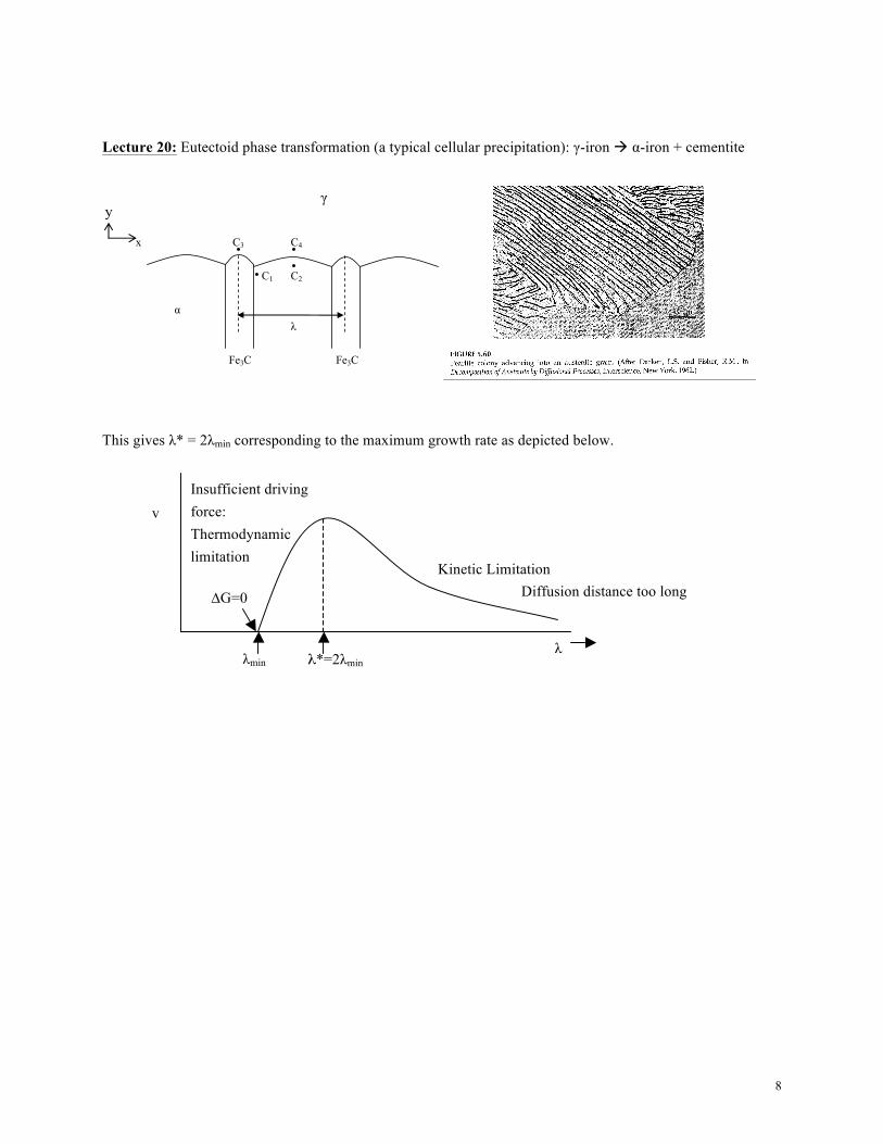
Note the similarity with cellular precipitation (see Lecture 20). In cellular precipitation, the lamellar spacing corresponding to the maximum growth rate is twice that of the minimum possible. As learned from Lecture 23, for the fluctuation to be stable (thermodynamically favorable) in relation to the original, homogeneous solid solution, we must have

0

2 22

2{ 2 } 04m

c

A gg Kc

β∂

Δ = + ≤∂

This also gives the critical β and λ, 0

21/ 2

2

1[ ( )]2c

c

gK c

β∂

= −∂

, 0

21/ 2

2 2

2 1[ ( )]8c

c c

gK c

πλ

β π−∂

= = −∂

Meaning, when λ < λC, or β > βC, Δg will become > 0, not thermodynamically favorable for the fluctuation to be stable, i.e., for the Spinodal decomposition to proceed.

βm β

βc

R(β)

12m cβ β=

λm λ

λc

2m cλ λ=

Thermodynamic

Limitation Kinetic (diffusion)

Limitation

R(λ) Thermodynamic

Limitation

Kinetic (diffusion)

Limitation

8

Lecture 20: Eutectoid phase transformation (a typical cellular precipitation): γ-iron à α-iron + cementite

x

α

Fe3C

C2

C3 C4

C1

λ

Fe3C

This gives λ* = 2λmin corresponding to the maximum growth rate as depicted below.

y γ

v

λmin λ*=2λmin λ

Insufficient driving force: Thermodynamic limitation

Kinetic Limitation Diffusion distance too long ∆G=0