Learning via Sequential Market Entry: Evidence fromInternational Releases of U.S. Movies∗

Isaac Holloway†

September 18, 2012

Abstract

New products tend to enter foreign markets sequentially. This paper proposes

a model in which firms do not initially know the true quality of their products, but

in order to enter a new market, the firm must pay a fixed cost. Each firm bases its

initial revenue forecasts on country and product characteristics, and each successive

release serves to update the firm’s expectations for future performance—and thus

its decision to enter more markets. On a sample of U.S. movies, I find that a one-

standard-deviation increase in the update to expected box-office revenues, based

on the previous round of entry, is associated with a 25% increase in the probability

of entry to a typical potential destination in the current round.

Keywords: heterogeneous quality; sequential entry; cultural goods trade

∗A version of this paper was included as Chapter 3 of my Ph.D. thesis at the University of BritishColumbia, entitled “Implications of Barriers to Trade for Exports of Cultural Goods and Services.” Iappreciate invaluable guidance from my supervisors Keith Head and John Ries. I also benefitted fromhelpful discussions with Hiro Kasahara, Barbara Spencer, and Chuck Weinberg. Any errors are mine.†School of Economics and Management, Tsinghua University, Beijing 100084, China. Tel: (86-010)

62793492, Email: isaac@sem.tsinghua.edu.cn

1 Introduction

New products are almost never released simultaneously around the world.1 Typically, a

product will be released domestically and then spread geographically over time. There

are a variety of reasons that might lead firms to delay the global distribution of a new

product. For instance, firms may choose to delay if domestic success contributes to a

positive “buzz”, which could be harnessed for international marketing efforts (Elberse

and Eliashberg, 2003; McCalman, 2005). Alternatively, if cash-poor firms have private

information about the quality of their products, they may not be able to convince creditors

to finance international expansion without the proof of robust domestic sales (Chaney,

2005; Manova, 2010; Minetti and Zhu, 2011). Or firms may be uncertain about their own

products’ profitability (Akhmetova, 2010; Albornoz et al., 2010; Eaton et al., 2011), and

thus each subsequent entry could serve to add information about the product’s appeal,

allowing the firm to update expectations in potential subsequent markets—and avoiding

costly entries where they are likely to fail.

At the heart of all three of these explanations is a lack of information, either on the part

of consumers, financiers, or the firms themselves. The recent papers cited above exemplify

the increased interest in the role of firm learning on the sequential nature of foreign

entry. In this paper, I use the motion picture industry to investigate the phenomenon of

sequential entry. I document facts about the spatial and temporal patterns of theatrical

releases of U.S. movies in key international markets, and propose a model of firm learning.

Taking into account the ex ante variability of performance within each market as well

as the correlations of performance across foreign markets, I find that a one-standard-

deviation increase in the update to expected box-office revenues, based on the previous

round of entry, is associated with a 25% increase in the probability of entry to a typical

potential destination in the current round.

1See, for example, Gatignon et al. (1989) and Ganesh et al. (1997) for marketing research oninternational diffusion by multinationals.

1

An additional alternative explanation applies to the motion picture industry. If some

factors of production are reusable, then staggering entry is a cost-saving exercise. The

prints on which films are encoded are expensive, costing about two thousand dollars each.2

To the extent that they can be reused in multiple countries, delaying international release

dates could allow for significant savings. Distributors could release in big markets first

and then spread to the smaller markets as prints become available. The marketing effort

of the stars—often in the form of local talk-show appearances—is also reusable, and of

course by its nature cannot take place simultaneously in distant locales. These tangible

examples from Hollywood serve to illustrate more general issues, such as managerial

attention to a product release. The alternative explanations of staggered entry do not

preclude the strategy that firms use sequential release dates to learn about their product

quality. It is possible that all of these concepts are at play. The empirical results of this

paper suggest that, even if sequential entry is due to other factors, distributors do learn

from their experiences, and act on them by entering more markets on good news and

fewer markets on bad news.

There are also forces that would contribute towards simultaneous release dates. Dis-

counting of the future implies firms would rather realize their profits sooner than later.

More importantly, delayed foreign release increases the potential for lost sales due to

piracy. Distributors face a trade-off between strategically delaying entry, and moving

to “day-and-date” simultaneous releases to combat international piracy. If firm learn-

ing is an important aspect of staggered release schedules, then the costs of simultaneous

international entry could be larger than previously thought.

This paper is related to the nascent literature on exporting and firm learning. Eaton

et al. (2011) (EEKKT, hereafter) observe in Columbian transaction-level data that many

firms export small amounts and have short tenure as exporters. These facts appear to

be inconsistent with the dominant theory of fixed-exporting costs introduced by Melitz

2Finney (2010).

2

(2003). If fixed costs are important, there should be a minimum scale required of ex-

porters in order to break even. EEKKT reconcile the facts with fixed-exporting costs by

introducing a search and learning model of trade, in which exporters are initially uncer-

tain of their products’ appeal in the foreign market. They estimate their model using the

U.S.–Columbia transaction data. Thus, the focus is on learning over time in a bilateral

setting. By contrast, the present study considers learning across foreign markets.

Albornoz et al. (2010) (ACCO, hereafter) similarly write a model in which exporters

are uncertain about their profitability of exporting. Theirs is a stylized model of two

countries and two periods, and emphasizes the value of information from entering one

market at a time. The empirical predictions derived from the model are indirect indi-

cations of firm learning. ACCO find supporting evidence from a census of Argentinean

manufacturers that, conditional on survival, growth rates are highest between the first

and second periods in the first export market of the firm. This pattern is consistent with

a firm that adjusts its supply upon receiving good news, assuming that the firm can learn

almost perfectly after one period. The empirical section of the present study directly tests

whether firms respond to past performances by including a Bayesian-derived updating

term in an entry regression. Moreover, correlations between markets are not perfect, and

differ from one country-pair to another.

Akhmetova (2010) introduces a model in which new exporters can choose a “testing

technology”, which allows them to export without paying fixed costs, but at a marginal

cost that is convex. A second technology exhibits linear marginal costs but requires the

payment of a one-time fixed cost of entry. Firms observe noisy signals about their demand

during the testing stage. The model endogenizes the length and intensity of the testing

stage and—like Arkolakis (2008) and EEKKT—the size of the second-stage entry cost.

In choosing the amount of investment in each period, the exporter takes into account the

expected revenues that will obtain, but also the value of the information that is learned.

3

This paper is most similar to ACCO, in that it investigates whether firms sequentially

add export destinations as a result of a learning strategy. The “firms” in this study

are motion pictures, however, and thus the industry context is quite different. Foreign

motion-picture revenue is trade in services (of the actors, directors, editors, etc.), as

opposed to the manufacturing trade that was the focus of the other papers. Moreover,

movies are cultural products, and thus subject to possibly wide differences in appeal

across markets. A necessary condition for firm learning is a positive correlation of appeal

in this dimension. ACCO allow for less-than-perfect correlation across markets in an

appendix, but focus on the case of single-period (perfect) learning. Furthermore, the

life cycle of an individual movie is much shorter than most traded goods. In any given

market, a movie will typically play for 4–6 weeks; in the sample of this paper, movies had

entered 95% of their ultimate markets within 12 months. Because of these features, firms

only make one entry decision per market; there is no scope for intra-market learning.

A key feature of this paper is that I track individual products (movies) and not just

firms that may sell multiple products. This is important because the theory relates to the

level of demand at the product level. A positive market response to one product may not

translate to a firm’s other offerings, so it is cleaner to have product-level data. Moreover,

the product does not improve over time, as a firm’s productivity might, and thus results

are not subject to that potential confounding factor. Secondly, in the empirical section

I directly test whether past surprises in revenue affect the current probability of further

entry. This contrasts with ACCO, who indirectly test learning by separating first-year

exporters from experienced (all other) exporters. I am also able to demonstrate the

validity of the exercise by showing that future (unrealized) surprises are not nearly as

salient as past surprises in explaining entry, which would have indicated that firms do

know their true quality—and anticipate the “surprises”—but stagger for other reasons.

The results suggest an additional cost to piracy. If distributors move toward simultaneous

4

release in order to thwart pirates, they lose the value of learning-by-staggering, and thus

may incur substantial fixed costs even if the movie turns out to have low appeal.

As discussed in the opening paragraph, there is a confluence of factors that inform

the international entry strategy of new products. The marketing literature has identi-

fied many of these issues for motion pictures,3 but little attention has been given to the

idea that distributors might be using a learning strategy to avoid bad investments. Nee-

lamegham and Chintagunta (1999) propose a Bayesian model of box-office forecasting,

in which projections for each movie-destination are updated as new information becomes

available. Crucially, however, they treat the decision of whether or not to release a

movie in a given country as exogenous. In contrast, I focus on how firms update their

expectations in order to inform the entry decision.

The paper proceeds as follows. In section 2 I describe the data set and document

features of the spatial-temporal pattern of entry for U.S. movies. In section 3 I derive a

model of firm learning that guides the empirical specifications that follow. The regres-

sions suggested by the model are estimated in section 4, along with tests for alternative

explanations and other robustness checks. The conclusion summarizes the main findings.

2 Data

Ticket sales revenue by country were collected from the web site boxofficemojo.com. The

full sample includes all U.S. movies that were shown in at least one of the other markets

considered over the period 2002-2008.4 Production budget data was taken from the

web site the-numbers.com and is available for 761 of the movies. Categorical variables,

including the main genre and MPAA rating were obtained from the-numbers.com and

3See Elberse and Eliashberg (2003) and Eliashberg, Elberse and Leenders (2006) and the referencestherein.

4The other 13 markets are Argentina, Australia, Czech Republic, France, Germany, Hong Kong, Italy,Japan, Netherlands, New Zealand, Norway, Spain, and United Kingdom.

5

imdb.com, respectively.

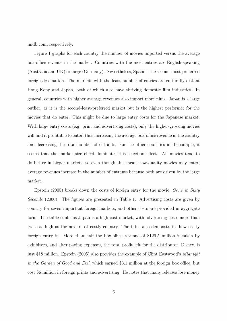
Figure 1 graphs for each country the number of movies imported versus the average

box-office revenue in the market. Countries with the most entries are English-speaking

(Australia and UK) or large (Germany). Nevertheless, Spain is the second-most-preferred

foreign destination. The markets with the least number of entries are culturally-distant

Hong Kong and Japan, both of which also have thriving domestic film industries. In

general, countries with higher average revenues also import more films. Japan is a large

outlier, as it is the second-least-preferred market but is the highest performer for the

movies that do enter. This might be due to large entry costs for the Japanese market.

With large entry costs (e.g. print and advertising costs), only the higher-grossing movies

will find it profitable to enter, thus increasing the average box-office revenue in the country

and decreasing the total number of entrants. For the other countries in the sample, it

seems that the market size effect dominates this selection effect. All movies tend to

do better in bigger markets, so even though this means low-quality movies may enter,

average revenues increase in the number of entrants because both are driven by the large

market.

Epstein (2005) breaks down the costs of foreign entry for the movie, Gone in Sixty

Seconds (2000). The figures are presented in Table 1. Advertising costs are given by

country for seven important foreign markets, and other costs are provided in aggregate

form. The table confirms Japan is a high-cost market, with advertising costs more than

twice as high as the next most costly country. The table also demonstrates how costly

foreign entry is. More than half the box-office revenue of $129.5 million is taken by

exhibitors, and after paying expenses, the total profit left for the distributor, Disney, is

just $18 million. Epstein (2005) also provides the example of Clint Eastwood’s Midnight

in the Garden of Good and Evil, which earned $3.1 million at the foreign box office, but

cost $6 million in foreign prints and advertising. He notes that many releases lose money

6

Figure 1: Intensive vs. Extensive Margins of Entry

abroad.

Figure 1 shows that there is wide variation at both the extensive and intensive margins

of entry. To understand which films are traveling abroad, consider Figure 2, which plots

the number of markets a movie enters against its domestic box-office revenue. Better-

performing movies tend to enter more foreign markets, and the relationship is tighter for

the non-comedy-drama genres. While there is considerable noise at the disaggregated

movie level, Figure 3 shows that, when movies are aggregated according to the number of

markets they entered, there is a monotonic relationship between the number of markets

and the mean domestic revenue.

Figures 2 and 3 tell us about the long-run pattern of entry. Not surprisingly, the more

appealing a movie is to audiences—as measured by domestic box-office returns—the more

countries that movie is likely to enter. This result is natural if destination-specific fixed

costs are important. Then only those movies that are likely to earn enough at the box-

7

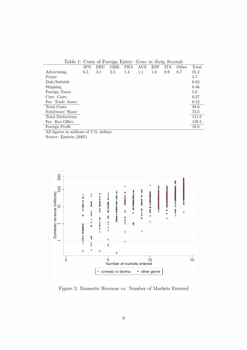
Table 1: Costs of Foreign Entry: Gone in Sixty SecondsJPN DEU GBR FRA AUS ESP ITA Other Total

Advertising 6.5 3.1 2.5 1.4 1.1 1.0 0.9 8.7 25.2Prints 5.7Dub/Subtitle 0.82Shipping 0.46Foreign Taxes 5.0Curr. Conv. 0.27For. Trade Assoc. 0.12Total Costs 38.0Exhibitors’ Share 73.5Total Deductions 111.5For. Box Office 129.5Foreign Profit 18.0All figures in millions of U.S. dollarsSource: Epstein (2005)

Figure 2: Domestic Revenue vs. Number of Markets Entered

8

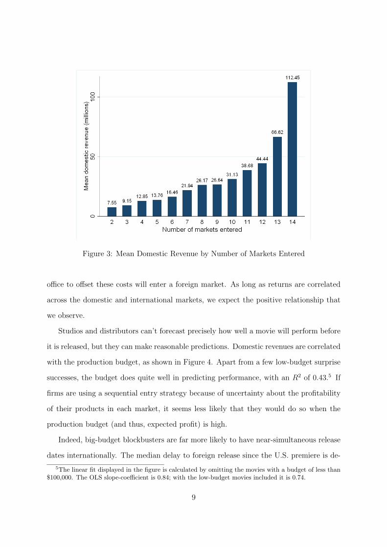
Figure 3: Mean Domestic Revenue by Number of Markets Entered

office to offset these costs will enter a foreign market. As long as returns are correlated

across the domestic and international markets, we expect the positive relationship that

we observe.

Studios and distributors can’t forecast precisely how well a movie will perform before

it is released, but they can make reasonable predictions. Domestic revenues are correlated

with the production budget, as shown in Figure 4. Apart from a few low-budget surprise

successes, the budget does quite well in predicting performance, with an R2 of 0.43.5 If

firms are using a sequential entry strategy because of uncertainty about the profitability

of their products in each market, it seems less likely that they would do so when the

production budget (and thus, expected profit) is high.

Indeed, big-budget blockbusters are far more likely to have near-simultaneous release

dates internationally. The median delay to foreign release since the U.S. premiere is de-

5The linear fit displayed in the figure is calculated by omitting the movies with a budget of less than$100,000. The OLS slope-coefficient is 0.84; with the low-budget movies included it is 0.74.

9

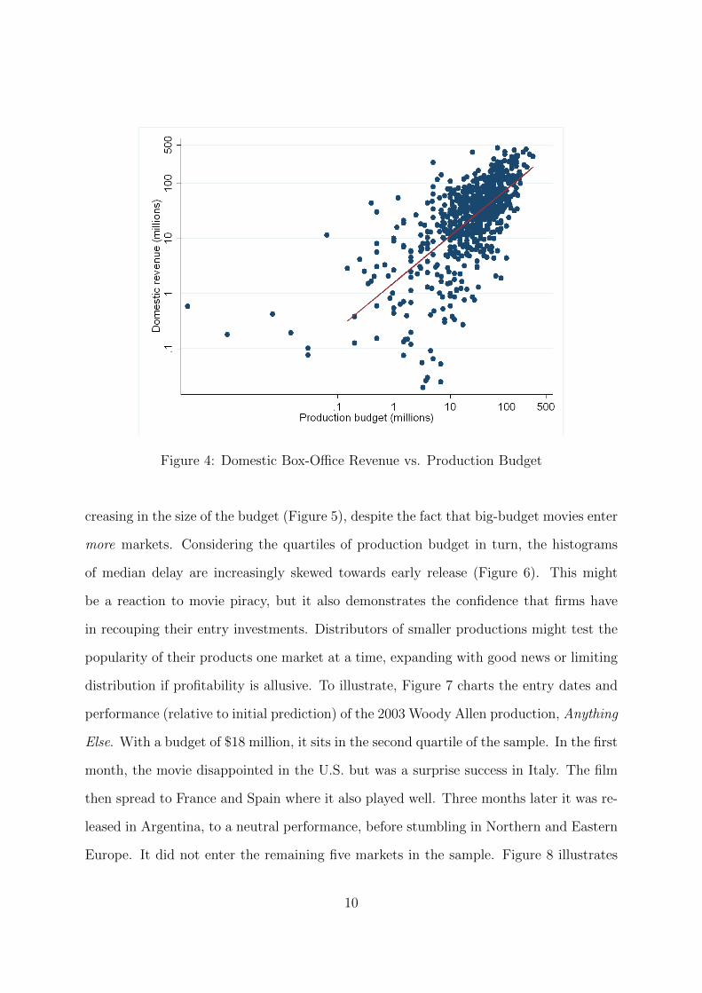
Figure 4: Domestic Box-Office Revenue vs. Production Budget

creasing in the size of the budget (Figure 5), despite the fact that big-budget movies enter

more markets. Considering the quartiles of production budget in turn, the histograms

of median delay are increasingly skewed towards early release (Figure 6). This might

be a reaction to movie piracy, but it also demonstrates the confidence that firms have

in recouping their entry investments. Distributors of smaller productions might test the

popularity of their products one market at a time, expanding with good news or limiting

distribution if profitability is allusive. To illustrate, Figure 7 charts the entry dates and

performance (relative to initial prediction) of the 2003 Woody Allen production, Anything

Else. With a budget of $18 million, it sits in the second quartile of the sample. In the first

month, the movie disappointed in the U.S. but was a surprise success in Italy. The film

then spread to France and Spain where it also played well. Three months later it was re-

leased in Argentina, to a neutral performance, before stumbling in Northern and Eastern

Europe. It did not enter the remaining five markets in the sample. Figure 8 illustrates

10

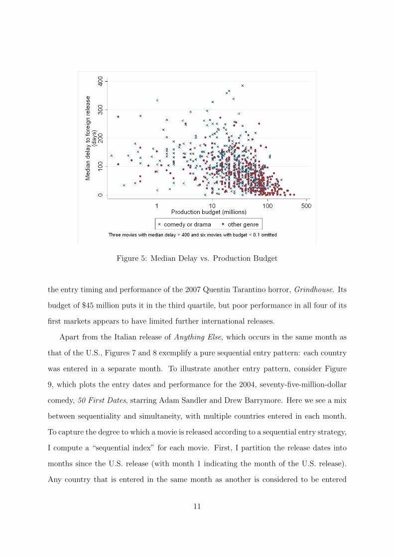
Figure 5: Median Delay vs. Production Budget

the entry timing and performance of the 2007 Quentin Tarantino horror, Grindhouse. Its

budget of $45 million puts it in the third quartile, but poor performance in all four of its

first markets appears to have limited further international releases.

Apart from the Italian release of Anything Else, which occurs in the same month as

that of the U.S., Figures 7 and 8 exemplify a pure sequential entry pattern: each country

was entered in a separate month. To illustrate another entry pattern, consider Figure

9, which plots the entry dates and performance for the 2004, seventy-five-million-dollar

comedy, 50 First Dates, starring Adam Sandler and Drew Barrymore. Here we see a mix

between sequentiality and simultaneity, with multiple countries entered in each month.

To capture the degree to which a movie is released according to a sequential entry strategy,

I compute a “sequential index” for each movie. First, I partition the release dates into

months since the U.S. release (with month 1 indicating the month of the U.S. release).

Any country that is entered in the same month as another is considered to be entered

11

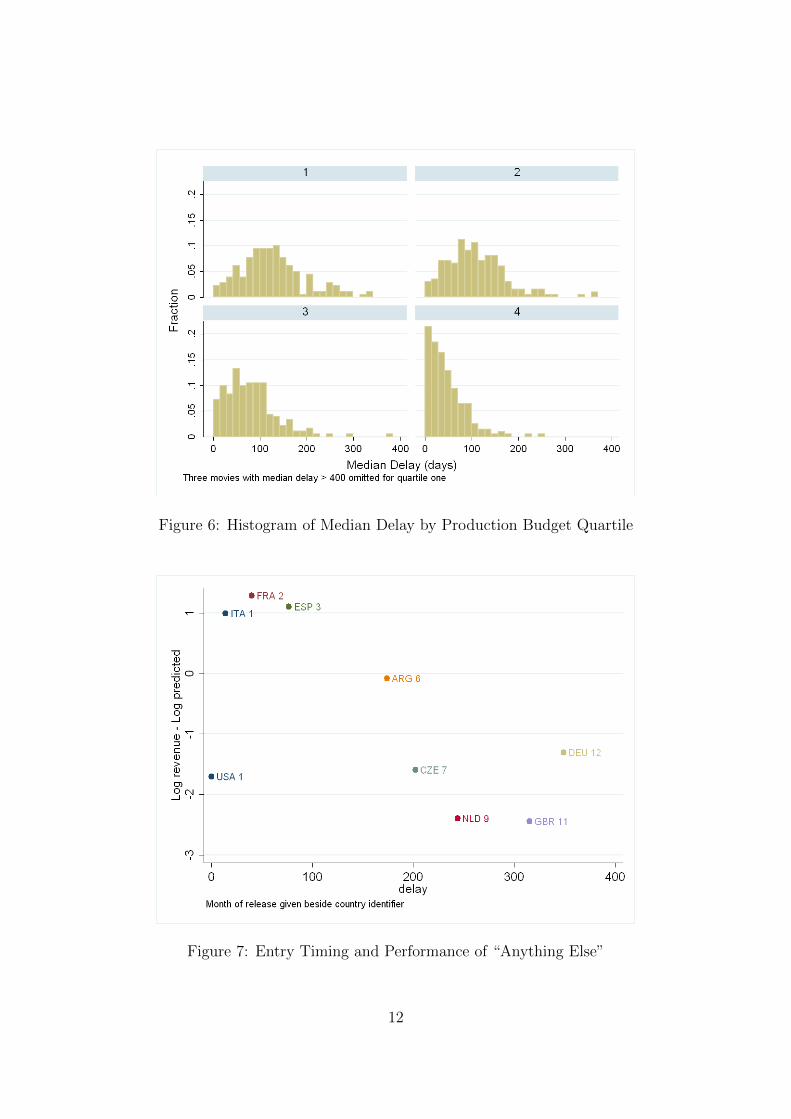
Figure 6: Histogram of Median Delay by Production Budget Quartile

Figure 7: Entry Timing and Performance of “Anything Else”

12

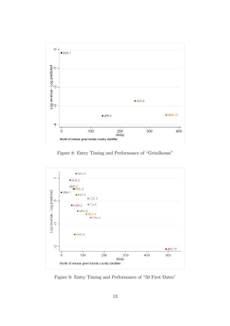
Figure 8: Entry Timing and Performance of “Grindhouse”

Figure 9: Entry Timing and Performance of “50 First Dates”

13

simultaneously with that other country. For most movies, there are gaps in the month in

which new entry occurs. For example, a movie might go to two markets in month one,

three markets in month two, but then only enter its last market in the fifth month. I

refer to months in which the movie does enter new markets as “rounds” of release, so for

this hypothetical movie, the fifth month would be considered round three. The sequential

index, Z, is computed as follows:

Z =Nrounds − 1

Nmarkets − 1, (1)

where Nrounds is the number of rounds of release and Nmarkets is the total number

of markets entered for each movie. The index gives the ratio of the number of extra

rounds taken to the number of foreign markets entered. Thus, if the movie enters ten

countries and takes ten rounds of release to do so, the fraction is one, and this movie

is characterized by pure sequential entry. If the movie entered all ten countries in one

round, the fraction would be zero, indicating pure simultaneous entry. Interior values

indicate the degree to which the movie followed a sequential entry strategy. For example,

consider a movie that entered five markets. If it did so in three rounds, the index is

(3− 1)/(5− 1) = 0.5, reflecting the fact that a mix of simultaneous and sequential entry

is observed.

Figure 10 provides a histogram of the sequential index. It shows a large spike at one,

reflecting the fact that more than one hundred of the movies exhibit pure sequential entry.

Just twenty of the movies were released according to a pure simultaneous strategy (all

within a month of the U.S. release). The remainder fall somewhat symmetrically around

a value of one half, with a small spike around the 0.2 mark.

We have established that movies with large production budgets tend to diffuse interna-

tionally more quickly. The longer delay for low-budget movies could be due to sequential

entry, or it could occur if they are delaying all their foreign releases for some time, and

14

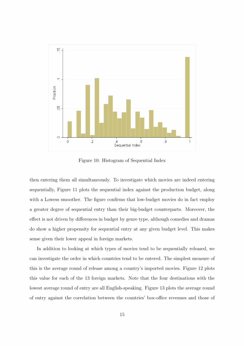
Figure 10: Histogram of Sequential Index

then entering them all simultaneously. To investigate which movies are indeed entering

sequentially, Figure 11 plots the sequential index against the production budget, along

with a Lowess smoother. The figure confirms that low-budget movies do in fact employ

a greater degree of sequential entry than their big-budget counterparts. Moreover, the

effect is not driven by differences in budget by genre type, although comedies and dramas

do show a higher propensity for sequential entry at any given budget level. This makes

sense given their lower appeal in foreign markets.

In addition to looking at which types of movies tend to be sequentially released, we

can investigate the order in which countries tend to be entered. The simplest measure of

this is the average round of release among a country’s imported movies. Figure 12 plots

this value for each of the 13 foreign markets. Note that the four destinations with the

lowest average round of entry are all English-speaking. Figure 13 plots the average round

of entry against the correlation between the countries’ box-office revenues and those of

15

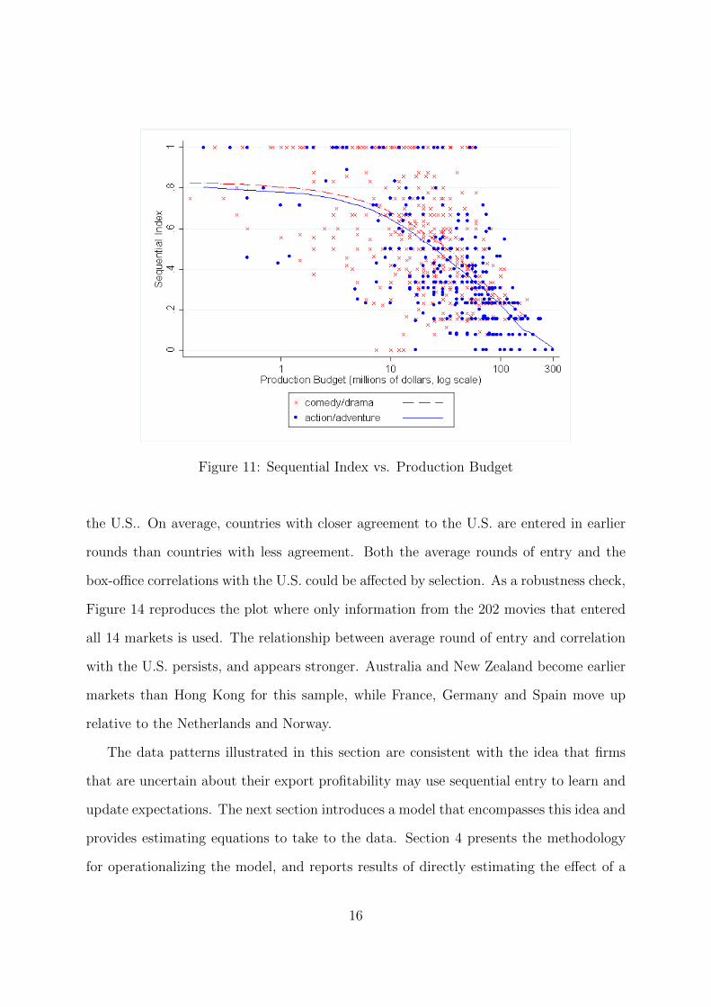
Figure 11: Sequential Index vs. Production Budget

the U.S.. On average, countries with closer agreement to the U.S. are entered in earlier

rounds than countries with less agreement. Both the average rounds of entry and the

box-office correlations with the U.S. could be affected by selection. As a robustness check,

Figure 14 reproduces the plot where only information from the 202 movies that entered

all 14 markets is used. The relationship between average round of entry and correlation

with the U.S. persists, and appears stronger. Australia and New Zealand become earlier

markets than Hong Kong for this sample, while France, Germany and Spain move up

relative to the Netherlands and Norway.

The data patterns illustrated in this section are consistent with the idea that firms

that are uncertain about their export profitability may use sequential entry to learn and

update expectations. The next section introduces a model that encompasses this idea and

provides estimating equations to take to the data. Section 4 presents the methodology

for operationalizing the model, and reports results of directly estimating the effect of a

16

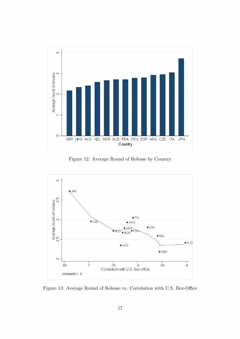
Figure 12: Average Round of Release by Country

Figure 13: Average Round of Release vs. Correlation with U.S. Box-Office

17

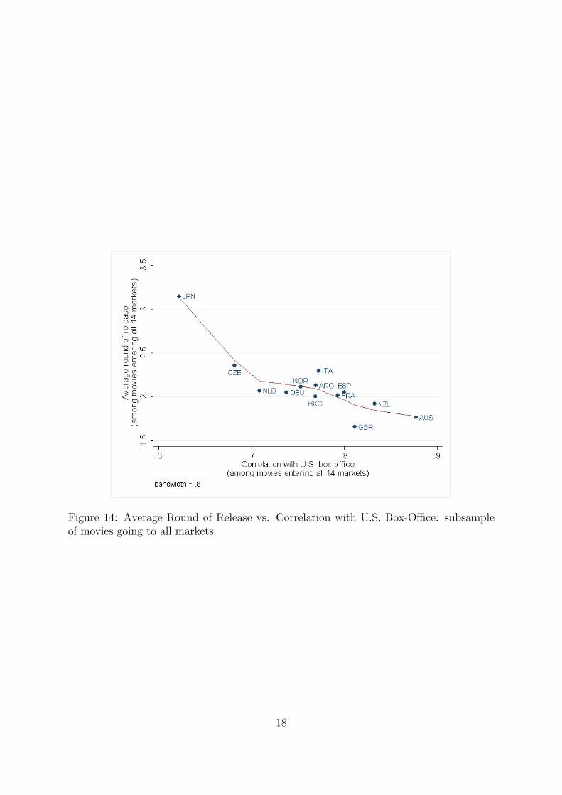
Figure 14: Average Round of Release vs. Correlation with U.S. Box-Office: subsampleof movies going to all markets

18

performance surprise on the probability of further entry.

3 Theory

Consider a risk-neutral firm making entry decisions in K segmented markets. To enter

any of the destination markets, indexed by d, firm m must incur a per-destination fixed

cost of Fdm, corresponding to print and advertising costs.

Movies are heterogeneous in their appeal, which is not directly observable even by

their distributors. The appeal of any given movie also varies between markets, due

to country-specific idiosyncracies in taste. Holloway (2011) introduces a discrete choice

model in which revenues for different varieties of a product (e.g. different movies) depend

on country- and variety-specific terms multiplicatively, in addition to a multiplicative

idiosyncratic factor. The derivation follows.

Individuals in country d purchase a variety of the product if their valuation of doing so

is greater than the price, pd, which varies between countries but not within each country.

Prices are taken as given in each market. The valuation of individual i from destination

d consuming variety m is:

vidm = k(βqm + ψdm + Uidm)n(yd), (2)

where qm is the average perceived quality of the variety, ψdm is the country-variety taste

shock, Uidm is the individual’s idiosyncratic utility, yd is the income per capita in country

d and the functions k(·) and n(·) are increasing and could be destination-country specific.

The parameter β adjusts for the scale on which quality is measured. Valuation is separable

in per capita income, reflecting the higher willingness-to-pay in rich countries for any given

quality level.

Revenues from exporting to country d are given as the product of the price and the

19

number of people who purchase the variety. This latter quantity can be expressed as the

product of the total population and the proportion of the public who purchase:

Rdm = pdMdP[vidm > pd], (3)

where Md is the population of country d and the proportion of the purchasing public is

replaced by the probability that any of the (symmetric) individuals in the country will

purchase.

Plugging 2 into 3,

Rdm = pdMdP[k(βqm + ψdm + Uidm)n(yd) > pd]

= pdMdP[βqm + Uidm + ψdm > k−1

(pd

n(yd)

)]

= pdMdP[Uidm > k−1

(pd

n(yd)

)− βqm − ψdm]

= pdMd(1− P[Uidm < k−1

(pd

n(yd)

)− βqm − ψdm]) (4)

If Uidm is distributed exponentially with parameter λ, then the above reduces to:

Rdm = pdMdeλ+βqm+ψdm−k−1

(pd

n(yd)

)(5)

Define the attractiveness of country d as Ad ≡ pdMdeλ−k−1

(pd

n(yd)

)and let Qm ≡ eqm

and Ψdm ≡ eψdm . We can then express the revenue equation succinctly as

Rdm = QβmAdΨdm. (6)

Taking the logarithm of equation (6) gives the linear equation,

rdm = βqm + ad + ψdm, (7)

20

where lower-case letters represent logarithmic terms and ψdm ∼ N(0, σ2ψ).

Although the quality of the movie is not known ex ante, there are known imperfect

proxies. A firm might make reasonable predictions about future revenues in each of the

prospective markets by substituting the known proxies in for unknown quality, and using

historical data to estimate country fixed effects—to substitute for ad—and the parameter

β. That is, if the firms know the “law of revenues”, they can substitute in their quality

proxies to make initial predictions about potential revenues in each of the markets. In

particular, suppose that quality, qm, is a function of the logarithm of the movie’s budget,

bm = lnBm:

qm = αbm + ξm, (8)

where ξm ∼ N(0, σ2ξ ). Substituting equation (8) into (7), and replacing ad by a set of

destination fixed effects gives6

rdm = βαbm + ad + νdm. (9)

where νdm = βξm + ψdm.

Firms form beliefs for each market according to equation (9).7 The normality assump-

tions on ξ and ψ—and thus on ν—imply a normal prior: rdm ∼ N(µdm1, σ2d1), where

µdm1 = βαbm + ad (10)

σ2d1 = σ2

νd. (11)

For clarity of exposition, let us assume there are only three destinations, A, B, and

C. All movies enter market A but the firms can choose whether or not to enter B and

C. After the first period, firms update their expectations about log revenues, rdm, in the

6By an abuse of notation, I am calling the destination-specific constant (fixed effect), ad, which is notequal to the conceptual lnAd.

7That is, firms know the value of the compound parameter βα and the destination-specific constants.

21

remaining potential markets, d ∈ {B,C}, using realized revenues in market A. According

to Bayes’ Law, rdm2 ∼ N(µdm2, σ2dm2) with

µdm2 = µdm1 + ρAdσd1σA1

(rAm − µAm1) (12)

σ2dm2 = σ2

d1(1− ρ2Ad) (13)

where ρAd is the correlation between νAm and νdm, σd1 is the square root of σ2νd

, and

(rAm − µAm1) ≡ νAm is the difference between the realized and expected log revenues for

movie m in country A.

These Bayesian updating formulas provide intuition for how predictions in future

potential markets depend on the surprises observed in entered markets. The surprises

are tempered by the degree of correlation across the two countries, and the degree of

variation within each of the countries. The posterior variance is always decreased after

new information is attained, but again the amount of precision gained depends on the

correlation between the markets involved.8

The model abstracts from the informational value of entering and is thus a model of

“passive” learning. The movie will enter market d if the expected profit from doing so is

positive. Recall that a fee of Fdm is required for movie m to enter market d. Assume that

Fdm = Kdζdm, where Kd is destination-specific but ζdm is movie-destination-specific and

is unobservable to the econometrician, though known to the firms. Letting Edmt denote

the indicator function for entry of m into d in period t, the probability that movie m will

8In practice, movies enter more than one country per period. To aggregate the surprises in each ofthe entered markets, a matrix version of Bayes’ Law is required. It is introduced in section 4.1.

22

enter destination d is9

P[Edmt = 1] = P[Et[Rdm − Fdm] > 0]

= P[Et[Rdm] > Kdζdm]

= P[eµdmt+σ2dmt

2 > Kdζdm]

= P[µdmt +σ2dmt

2> logKd + logζdm]

= P[logζdm < µdmt +σ2dmt

2− logKd]

= P[logζdm < µdm,t−1 + sdm,t−1 +σ2dmt

2− logKd], (14)

where sdm,t−1 is the update based on last period’s performance.

Note that the variance terms become movie specific after the first period. This is

because not all movies enter countries in the same order. Since the updated variance de-

pends on the correlation coefficient between the country in consideration and the country

of last entry, the variance terms will differ if the country of last entry differs. In the

simple three-country example, country B for one movie may be country C for another.

4 Results

The model predicts that surprises in box-office revenue in previous markets affect the

probability of entry into potential future markets. I test this prediction using regression

analysis and consider alternative explanations for the results.

4.1 Firm learning and the decision to enter

First it is necessary to construct the appropriate variables, in particular the update

to movie m at time t. Recall from the model that, initially, distributors form expected

9If log(X) ∼ N(µ, σ2) then X ∼ Log-N(µ, σ2) and EX = e(µ+σ2

2 ).

23

revenues for each potential destination based on movie characteristics such as the budget,

and destination characteristics such as the country’s historical expenditure on movies. I

form ex ante predicted revenues for each movie-destination pair by regressing ex post

actual (log) revenues on the movies’ (log) budget and destination fixed effects. I allow

the coefficient on budget to differ across the destinations and augment the equation with

interactions between country dummies and genre and MPAA-rating dummies:

lnRdm = αd lnBm + {FEd} × {GENREm}+ {FEd} × {MPAAm}+ {FEd}+ εdm. (15)

I then set the first-period predicted log revenues, µ1dm, equal to l̂nRdm.

Time periods are based on the month since the U.S. release. Although I have data on

the precise day on which a movie was released in any given market, it is impractical to

use days as the unit of time. Using daily time periods would introduce a lot of noise since

there may be many idiosyncratic reasons for releasing on one day rather than the next.

Recalling that the benefit to “pulling the plug” on a release is the saved fixed costs, the

incentive to do so decreases as the period between learning that the movie will not make

money in the market and the release date narrows. This is because advertising costs are

sunk once they are spent. Similarly, adding a new market based on good performance

would take time to organize and promote. I set the unit of time to be a month (30 days),

but robustness checks show the qualitative conclusions are unaffected by changing this

window.

For most movies, there are gaps in the month in which new entry occurs. For example,

a movie might go to two markets in month one, three markets in month two, but then

only enter its last market in the fifth month. According to the updating theory, there

is no explanation for the delay in entry to the fifth month. The same information was

available in the third and fourth months. Indeed, the model is about information sets

and not time. Accordingly, I collapse the data to the level of information sets—or rounds

24

of entry—rather than keep all possible months for each movie. Thus, for the hypothetical

movie above, only observations corresponding to months one, two, and five would be kept.

A final set of observations represents the round after the last new entry has taken place.

It is important to include since it is informative that none of the remaining potential

markets imported the movie in this last information set. This procedure highlights the

fact that we are not trying to explain the magnitude of the delay to foreign release, but

rather to test whether new information affects the decision to release.

I compute the expected revenues and surprises for each destination-movie-round triple

using an iterative procedure. The updating equations of section 3 apply if only one

country is entered per period. In practice, many movies enter multiple countries per

round and the surprises from each entered country must be aggregated to form the update

for each remaining potential market. To do this we can employ the matrix versions of

the Bayesian updating equations. Denote the set of countries entered in period t− 1 by

Y and the set of remaining potential destinations X.10 The updating equations become:

µtX = µt−1X + Σt−1

XY

(Σt−1Y Y

)−1 (rY − µt−1

Y

)(16)

ΣtXX = Σt−1

XX − Σt−1XY

(Σt−1Y Y

)−1 (Σt−1XY

)′, (17)

where µtX and µtY are vectors of predicted log revenues going into period t for the sets

X and Y , respectively, rY is the vector of realized log revenues in Y , ΣtXX and Σt

Y Y are

variance-covariance matrices, and Σt−1XY is a cross-covariance matrix. All initial variance

and covariance elements are calculated from the residuals, εdm, from equation (15).

Table 2 provides correlation coefficients of εdm for each country pair. On the main di-

agonal, the variance of the residuals within each country is reported. The upper triangle

reports Pearson correlation coefficients, which describe the strength of the linear relation-

10These sets of course depend on the movie, m, and the period, t, but the subscripts are omittedfor convenience of exposition. Note that the set of destinations entered before t − 1 is irrelevant to thecalculations since information from these entries is already incorporated into the t− 1 prior.

25

ships, and are directly related to the covariances between countries. The country-pair

with the highest correlation is Australia–New Zealand, at 0.768, followed by Australia–

United Kingdom (0.744) and Netherlands–Norway (0.743). The country-pair with the

lowest correlation is France–United States, at 0.396. The next three lowest correlations

also involve the United States, paired with Spain and Italy (each at 0.402) and Japan

(0.414). In general, the correlations point to regional and colonial groupings: there are

high correlations among Northern European and North American markets (U.S. statistics

include box-office revenue in Canada); Mediterranean European countries exhibit high

correlation among themselves; the market in most agreement with Japan is Hong Kong;

Argentina’s ties to Spain and Italy are reflected, although its second highest correlation

is surprisingly with Hong Kong. The lower triangle reports Kendall’s tau, which provides

a non-parametric measure of concordance of the ranking of movies for each country pair.

The same general patterns of association are uncovered through this alternative measure.

26

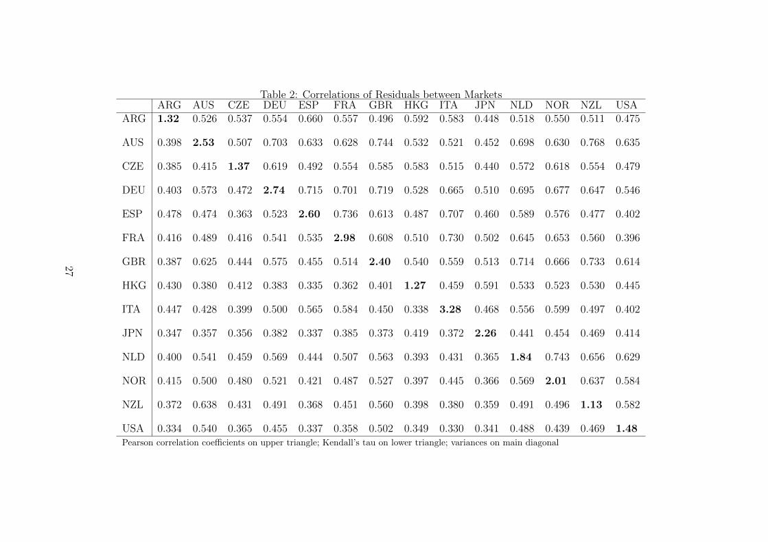
Table 2: Correlations of Residuals between MarketsARG AUS CZE DEU ESP FRA GBR HKG ITA JPN NLD NOR NZL USA

ARG 1.32 0.526 0.537 0.554 0.660 0.557 0.496 0.592 0.583 0.448 0.518 0.550 0.511 0.475

AUS 0.398 2.53 0.507 0.703 0.633 0.628 0.744 0.532 0.521 0.452 0.698 0.630 0.768 0.635

CZE 0.385 0.415 1.37 0.619 0.492 0.554 0.585 0.583 0.515 0.440 0.572 0.618 0.554 0.479

DEU 0.403 0.573 0.472 2.74 0.715 0.701 0.719 0.528 0.665 0.510 0.695 0.677 0.647 0.546

ESP 0.478 0.474 0.363 0.523 2.60 0.736 0.613 0.487 0.707 0.460 0.589 0.576 0.477 0.402

FRA 0.416 0.489 0.416 0.541 0.535 2.98 0.608 0.510 0.730 0.502 0.645 0.653 0.560 0.396

GBR 0.387 0.625 0.444 0.575 0.455 0.514 2.40 0.540 0.559 0.513 0.714 0.666 0.733 0.614

HKG 0.430 0.380 0.412 0.383 0.335 0.362 0.401 1.27 0.459 0.591 0.533 0.523 0.530 0.445

ITA 0.447 0.428 0.399 0.500 0.565 0.584 0.450 0.338 3.28 0.468 0.556 0.599 0.497 0.402

JPN 0.347 0.357 0.356 0.382 0.337 0.385 0.373 0.419 0.372 2.26 0.441 0.454 0.469 0.414

NLD 0.400 0.541 0.459 0.569 0.444 0.507 0.563 0.393 0.431 0.365 1.84 0.743 0.656 0.629

NOR 0.415 0.500 0.480 0.521 0.421 0.487 0.527 0.397 0.445 0.366 0.569 2.01 0.637 0.584

NZL 0.372 0.638 0.431 0.491 0.368 0.451 0.560 0.398 0.380 0.359 0.491 0.496 1.13 0.582

USA 0.334 0.540 0.365 0.455 0.337 0.358 0.502 0.349 0.330 0.341 0.488 0.439 0.469 1.48Pearson correlation coefficients on upper triangle; Kendall’s tau on lower triangle; variances on main diagonal

27

Table 3 reports the main result of the study. Each specification estimates the probabil-

ity that a movie enters a destination in a given round, conditional on the movie not being

released there previously. The table reports standardized average partial effects, so that

it presents the change in the probability of release induced by a one-standard-deviation

increase of the variable in question. The first column estimates the degree to which

current expected revenue affects the decision to release. The first round of releases is

excluded from the regression because this specification acts as a benchmark for the other

columns, which include lagged variables. The coefficient implies that a one-standard-

deviation increase in the (log) predicted revenue increases the probability of entry in the

current period by 14.8 percentage points, compared to an average probability of 21.3%.

As predicted, expected revenue makes a big difference in the decision to release a movie

in a given country.

The second specification examines the constituent parts of the expected revenue,

namely the expected log revenue in the previous round plus the update from the previous

period. If firms do not adapt their entry strategies based on information learned in

period (t− 1) then we should not expect the coefficient on the update to be significant.

In fact, the coefficient implies that a one-standard-deviation increase in the previous

round’s update is associated with a 5.0 percentage-point increase in the probability of

entry. This is an increase of more than 23% over the average probability of entry. Column

3 includes interactions between the update and dummies for the first period and all other

periods. This specification checks whether firms are learning only after the first round of

entry, or whether subsequent entries also affect entry decisions. The coefficients on the

interactions are nearly identical, suggesting that learning is ongoing.

Columns 4 and 5 investigate whether the effect of a surprise in a movie’s performance

depends on whether the surprise is positive or negative. Column 4 indicates that the

increase in the probability of entry due to positive news is more than twice as large in

28

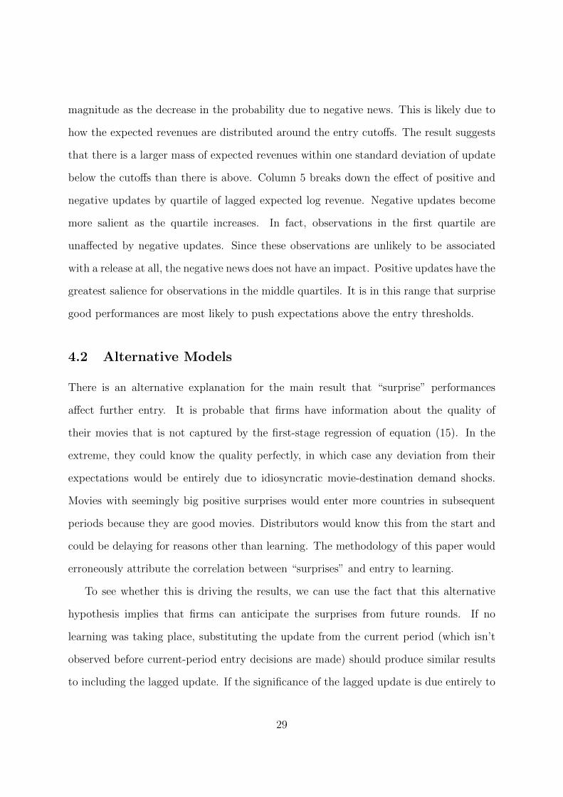
magnitude as the decrease in the probability due to negative news. This is likely due to

how the expected revenues are distributed around the entry cutoffs. The result suggests

that there is a larger mass of expected revenues within one standard deviation of update

below the cutoffs than there is above. Column 5 breaks down the effect of positive and

negative updates by quartile of lagged expected log revenue. Negative updates become

more salient as the quartile increases. In fact, observations in the first quartile are

unaffected by negative updates. Since these observations are unlikely to be associated

with a release at all, the negative news does not have an impact. Positive updates have the

greatest salience for observations in the middle quartiles. It is in this range that surprise

good performances are most likely to push expectations above the entry thresholds.

4.2 Alternative Models

There is an alternative explanation for the main result that “surprise” performances

affect further entry. It is probable that firms have information about the quality of

their movies that is not captured by the first-stage regression of equation (15). In the

extreme, they could know the quality perfectly, in which case any deviation from their

expectations would be entirely due to idiosyncratic movie-destination demand shocks.

Movies with seemingly big positive surprises would enter more countries in subsequent

periods because they are good movies. Distributors would know this from the start and

could be delaying for reasons other than learning. The methodology of this paper would

erroneously attribute the correlation between “surprises” and entry to learning.

To see whether this is driving the results, we can use the fact that this alternative

hypothesis implies that firms can anticipate the surprises from future rounds. If no

learning was taking place, substituting the update from the current period (which isn’t

observed before current-period entry decisions are made) should produce similar results

to including the lagged update. If the significance of the lagged update is due entirely to

29

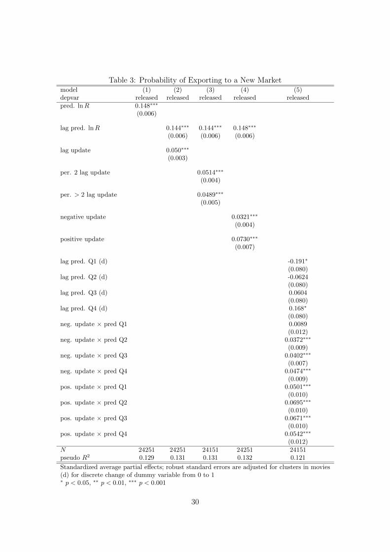
Table 3: Probability of Exporting to a New Marketmodel (1) (2) (3) (4) (5)depvar released released released released releasedpred. lnR 0.148∗∗∗

(0.006)

lag pred. lnR 0.144∗∗∗ 0.144∗∗∗ 0.148∗∗∗

(0.006) (0.006) (0.006)

lag update 0.050∗∗∗

(0.003)

per. 2 lag update 0.0514∗∗∗

(0.004)

per. > 2 lag update 0.0489∗∗∗

(0.005)

negative update 0.0321∗∗∗

(0.004)

positive update 0.0730∗∗∗

(0.007)

lag pred. Q1 (d) -0.191∗

(0.080)lag pred. Q2 (d) -0.0624

(0.080)lag pred. Q3 (d) 0.0604

(0.080)lag pred. Q4 (d) 0.168∗

(0.080)neg. update × pred Q1 0.0089

(0.012)neg. update × pred Q2 0.0372∗∗∗

(0.009)neg. update × pred Q3 0.0402∗∗∗

(0.007)neg. update × pred Q4 0.0474∗∗∗

(0.009)pos. update × pred Q1 0.0501∗∗∗

(0.010)pos. update × pred Q2 0.0695∗∗∗

(0.010)pos. update × pred Q3 0.0671∗∗∗

(0.010)pos. update × pred Q4 0.0542∗∗∗

(0.012)N 24251 24251 24151 24251 24151pseudo R2 0.129 0.131 0.131 0.132 0.121

Standardized average partial effects; robust standard errors are adjusted for clusters in movies(d) for discrete change of dummy variable from 0 to 1∗ p < 0.05, ∗∗ p < 0.01, ∗∗∗ p < 0.001

30

learning, then the current-round update should not enter significantly. The first column

of Table 4 estimates the effect of current expected log revenues on the probability of entry.

The difference from column 1 of Table 3 is that first-round observations are included in

the regression. This is to act as a benchmark for the specification of column 2, which

includes the current predicted log revenue and the update derived from current entries.

Column 2 indicates that a one-stand-deviation increase in the current update increases

the probability of entry by 0.85 percentage points. This suggests that firms do have some

information not accounted for in the initial forecast equation, but the estimated effect is

about one-sixth of the estimate for lagged updates, which is reproduced in column 3 for

convenience. The fact that the effect of lagged updates is so much stronger than current

(unrealized) updates suggests that we should not abandon the learning hypothesis.

In column 4, the variance of the prior distribution of log revenues is included. Recall

from equation (14) of section 3 that we expect the variance to enter positively. Mechan-

ically, this is because the logarithm of the expected revenue is the expected log revenue

plus one half the variance of log revenue if revenue is distributed log-normally. Intu-

itively, firms prefer to enter when the variance is high because their potential losses are

capped by the entry cost but there is no bound on the up side. Thus the combination

of the assumption of risk-neutral preferences on the part of firms and log-normally dis-

tributed conditional revenues provides the hypothesis that the variance term should enter

positively. Column 4 of Table 4 shows that high-variance observations are actually less

likely to be associated with entry. There are a couple of possible explanations to this

finding. First, firms may in fact be risk averse. Goettler and Leslie (2004) note that

industry-insiders claim to treat risky movies differently in their study of cofinancing in

the motion picture industry. In that paper, it is the studios’ decisions of how to finance

the movies’ production that is at issue. The authors point out that risk-averse behavior

is not expected for publically-owned firms, since shareholders can diversify risk through

31

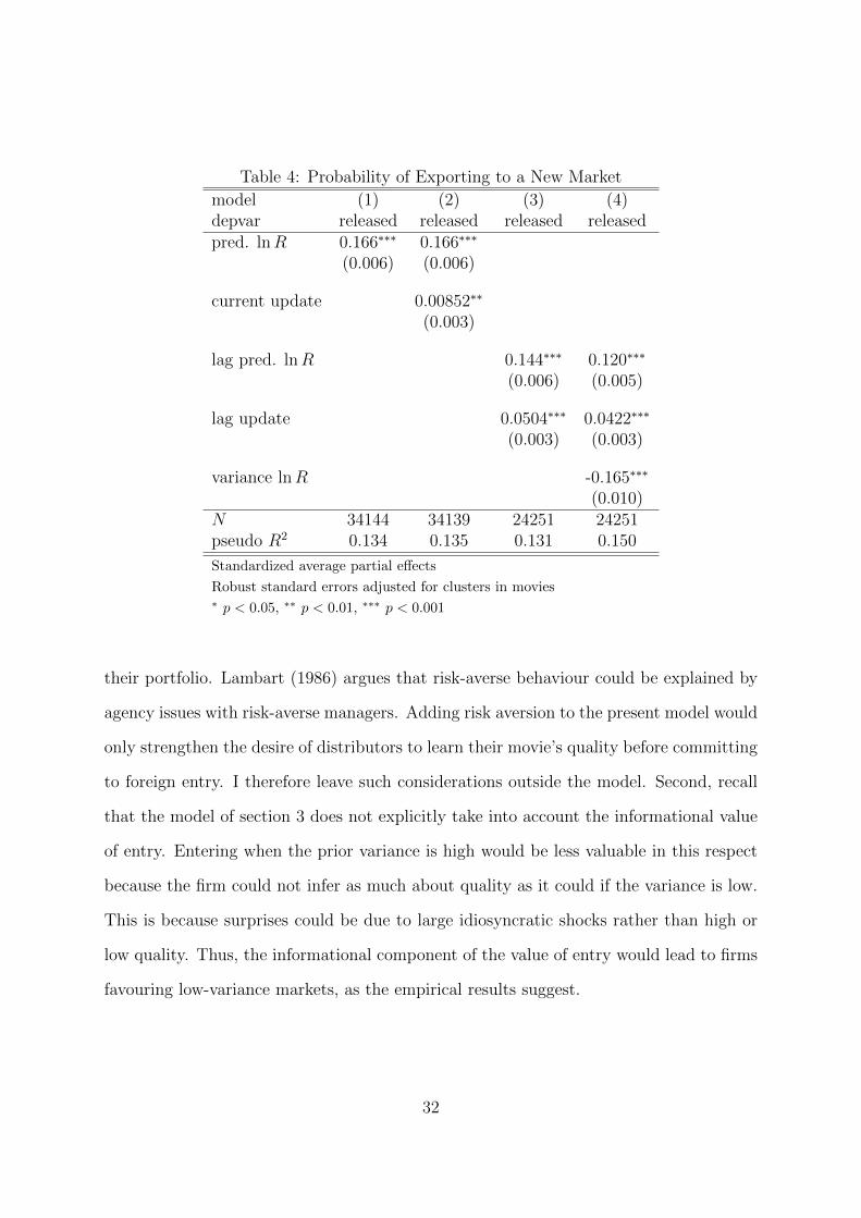
Table 4: Probability of Exporting to a New Market

model (1) (2) (3) (4)depvar released released released releasedpred. lnR 0.166∗∗∗ 0.166∗∗∗

(0.006) (0.006)

current update 0.00852∗∗

(0.003)

lag pred. lnR 0.144∗∗∗ 0.120∗∗∗

(0.006) (0.005)

lag update 0.0504∗∗∗ 0.0422∗∗∗

(0.003) (0.003)

variance lnR -0.165∗∗∗

(0.010)N 34144 34139 24251 24251pseudo R2 0.134 0.135 0.131 0.150

Standardized average partial effects

Robust standard errors adjusted for clusters in movies∗ p < 0.05, ∗∗ p < 0.01, ∗∗∗ p < 0.001

their portfolio. Lambart (1986) argues that risk-averse behaviour could be explained by

agency issues with risk-averse managers. Adding risk aversion to the present model would

only strengthen the desire of distributors to learn their movie’s quality before committing

to foreign entry. I therefore leave such considerations outside the model. Second, recall

that the model of section 3 does not explicitly take into account the informational value

of entry. Entering when the prior variance is high would be less valuable in this respect

because the firm could not infer as much about quality as it could if the variance is low.

This is because surprises could be due to large idiosyncratic shocks rather than high or

low quality. Thus, the informational component of the value of entry would lead to firms

favouring low-variance markets, as the empirical results suggest.

32

5 Conclusion

A growing body of work has suggested that manufacturing firms learn about their export

profitability through exporting. This paper adds to that literature by considering a new

type of product. Motion picture distributors only release a movie once in any destination

country, and thus have limited scope for intra-market learning. Furthermore, potentially

large idiosyncratic differences in taste across markets mean inferences from observed

performance must be far from perfect. Nonetheless, the results of this study suggest that

distributors do adjust their entry strategies based on prior-market performance, adding

markets after surprise successes and limiting further distribution after disappointments.

The correlation between past surprises and entry decisions could be due to omitted

movie attributes in the initial forecasts. Movies with positive unobserved attributes

will both perform better than expected (by the econometrician) and subsequently enter

more foreign markets. Robustness checks suggest this is likely a factor, but unrealized

surprises’ effect on entry decisions is just one-sixth the size of past surprises, leading to

the conclusion that learning is indeed taking place.

One limitation of this study is that the information value of delaying entry is not

explicitly modeled, nor accounted for in the empirics. Prior theoretical work has modeled

this option value, but these studies have relied on other simplifications to make modelling

trackable. Simplifications include limiting the analysis to two countries (Albornoz et al.,

2010), limiting uncertainty to a binary distribution ( Akhmetova, 2010), or restricting the

correlation of demand between countries to be equal across country-pairs (Nguyen, 2012).

Indirect evidence of strategic delay is found in the present study by inspecting the effect

of prior distribution variance on entry decisions. Risk-neutral firms prefer high variance if

entry is made myopically because their losses are capped at the cost of entry but there is

no bound on the up side. However, if firms use entry to learn about demand in potential

future destinations, lower variances provide a higher information value. Empirical results

33

suggest the latter effect to be at work.

As firms move toward a simultaneous release strategy to combat international piracy,

they lose the ability to use the information from prior markets. Thus, firms face a trade-

off between foregone revenues to illegal consumption if they delay foreign entry on the one

hand, and potentially loss-making foreign entries if they enter all markets simultaneously

on the other hand. Firm behavior is consistent with this trade-off: big-budget movies

which are likely to draw higher box-office returns are much more likely to enter foreign

markets simultaneously than smaller-budget movies that could be on the cusp of the

break-even point.

34

References

Akhmetova, Z., 2010, “Firm Experimentation in New Markets,” mimeo.

Albornoz, F, H.F. Calvo Pardo, G. Corcos, and E. Ornelas, 2010, “Sequential Export-ing,” mimeo.

Arkolakis, 2010, “Market Penetration Costs and the New Consumers Margin in Inter-national Trade,” Journal of Political Economy, 118(6), 1151-1199.

Chaney, T., 2005, “Liquidity Constrained Exporters,” University of Chicago mimeo.

Eaton, J., M. Eslava, C. J. Krizan, M. Kugler, and J. Tybout, 2011, “A Search andLearning Model of Export Dynamics,” mimeo.

Elberse, A. and J. Eliashberg, 2003, “Demand and Supply Dynamics for SequentiallyReleased Products in International Markets: The Case of Motion Pictures,” Mar-keting Science, 22(3), 329-354.

Eliashberg, J., A. Elberse and M. Leenders, 2006, “The Motion Picture Industry: Crit-ical Issues in Practice, Current Research, and New Directions,” Marketing Science,25(6), 638-661.

Epstein, E.J., 2005, “Send in the Aliens: They’re the last hope for the foreign boxoffice,” Slate, http://www.slate.com/id/2125153.

Finney, A., 2010, The International Film Business: A Market Guide Beyond Hollywood,Routledge, New York.

Ganesh, J., V. Kumar and V. Subramaniam, 1997, “Learning effect in multinationaldiffusion of consumer durables: An exploratory investigation,” J. Acad. MarketingSci., 25(3) 214-228.

Gatignon, H., J. Eliashberg and T. S. Robertson, 1989, “Modeling multinational diffu-sion patterns: An efficient methodology,” Marketing Science, 8(3) 231-247.

Goettler, R. and and P. Leslie, 2005, “Cofinancing to Manage Risk in the Motion PictureIndustry,” Journal of Economics & Management Strategy, 14(2), 231-261.

Holloway, I.R., 2011, “Foreign Entry, Quality, and Cultural Distance: Product-LevelEvidence from U.S. Movie Exports,” mimeo.

Lambert, R.A., 1986, “Executive Effort and Selection of Risky Projects,” RAND Journalof Economics, 17(1), 77-88.

Manova, K., 2010, “Credit Constraints, Heterogeneous Firms, and International Trade,”NBER Working Paper 14531.

35

McCalman, P., 2005, “International Diffusion and Intellectual Property Rights: AnEmpirical Analysis,” Journal of International Economics, 67, 353-372.

Melitz, M. J., 2003, “The Impact of Trade on Intra-Industry Reallocations and Aggre-gate Industry Productivity,” Econometrica 71(6), 1695-1725.

Minetti, R. and S. Zhu, 2011, “Credit Constraints and Firm Export: MicroeconomicEvidence from Italy,” Journal of International Economics, 83(2), 109-125.

Neelamegham, R. and P. Chintagunta, 1999, “A Bayesian Model to Forecast New Prod-uct Performance in Domestic and International Markets,” Marketing Science, 18(2),115-136.

Nguyen, D.X., 2012, “Demand Uncertainty: Exporting Delays and Exporting Failures,”Journal of International Economics, 86(2), 336-344.

36