Learning to See:Genetic and Environmental Influences

on Visual Development

James A. Bednar

Report AI-TR-02-294 May 2002

jbednar@cs.utexas.eduhttp://www.cs.utexas.edu/users/nn/

Artificial Intelligence LaboratoryThe University of Texas at Austin

Austin, TX 78712

Copyright

by

James Albert Bednar

2002

The Dissertation Committee for James Albert Bednarcertifies that this is the approved version of the following dissertation:

Learning to See:Genetic and Environmental Influences on Visual Development

Committee:

Risto Miikkulainen, Supervisor

Wilson S. Geisler

Raymond Mooney

Benjamin Kuipers

Joydeep Ghosh

Les Cohen

Learning to See:

Genetic and Environmental Influences on Visual Development

by

James Albert Bednar, B.S., B.A., M.A.

Dissertation

Presented to the Faculty of the Graduate School of

The University of Texas at Austin

in Partial Fulfillment

of the Requirements

for the Degree of

Doctor of Philosophy

The University of Texas at Austin

May 2002

Acknowledgments

This thesis would not have been possible without the support, advice, and encouragement of RistoMiikkulainen over the years, not to mention all his work on the draft revisions. If by some strokeof fate you have an opportunity to work with Risto, you should take it. I am also thankful forencouragement, constructive criticism, and career guidance from my incredibly wise committeemembers, Bill Geisler, Ray Mooney, Ben Kuipers, Joydeep Ghosh, and Les Cohen. Les Cohen inparticular provided much-needed insight into the infant psychology literature. Bill Geisler has beenvery patient and thoughtful regarding my biological interests and with rough drafts of several thesesand papers, and has provided valuable pointers to research in other fields.

I thank the members and all the hangers-on of the UTCS Neural Networks research groupfor invaluable feedback and many productive and entertaining discussions, especially YoonsuckChoe, Lisa Kaczmarczyk, Marty and Coquis Mayberry, Lisa Redford, Amol Kelkar, Tal Tversky,Bobby Bryant, Tino Gomez, Adrian Agogino, Harold Chaput, Paul McQuesten, Jeff Provost, andKen Stanley. Yoonsuck Choe in particular has long been a source of hard-hitting and constructivefeedback, as well as an expert resource for operating systems and hardware maintenance, and agood friend. Lisa Kaczmarczyk provided very helpful comments on earlier paper drafts, and I haveenjoyed having both of the Lisas as colleagues and friends. I have also benefitted from discussionsand get-togethers with a diverse, talented, and personable set of visitors to our group, including IgorFarkas, Alex Lubberts, Nora Aguirre, Daniel Polani, Yaron Silbermann, Enrique Muro, and AlexConradie.

I am very grateful for comments on research ideas and paper drafts from Mark H. Johnson,Harel Shouval, Francesca Acerra, Cara Cashon, Cornelius Weber, Dan Butts, and those who partic-ipated in the “Cortical Map Development” workshop at CNS*01. Joseph Sirosh provided the initialsoftware code used in my work, and I am also grateful to Harel Shouval, Bernard Achermann, andHenry Rowley for making their face and natural scene databases available.

I am very fortunate to have a loving and supportive family, and I thank each of them forpretending to believe me each semester that I promised to finish the dissertation. In particular, myparents Eugene D. and Julia M. Bednar have been a constant source of encouragement, and mygrandmothers Angelina Bednar and Julia D. Hueske have been a much-needed source of both moraland occasionally financial support. Throughout it all, the lovely and talented Tasca Shadix has kept

v

me going, and Patrick Sullivan, Amanda Toering, Jaime Becker, Tiffany Wilson, and Amy Storyhave provided friendship and distraction.

This research was supported in part by the National Science Foundation under grants #IRI-9309273 and #IIS-9811478. Computer time for exploratory simulations was provided by the TexasAdvanced Computing Center at the University of Texas at Austin and the Pittsburgh Supercomput-ing Center.

JAMES A. BEDNAR

The University of Texas at AustinMay 2002

vi

Learning to See:

Genetic and Environmental Influences on Visual Development

Publication No.

James Albert Bednar, Ph.D.The University of Texas at Austin, 2002

Supervisor: Risto Miikkulainen

How can a computing system as complex as the human visual system be specified and constructed?Recent discoveries of widespread spontaneous neural activity suggest a simple yet powerful ex-planation: genetic information may be expressed as internally generated training patterns for ageneral-purpose learning system. The thesis presents an implementation of this idea as a detailed,large-scale computational model of visual system development. Simulations show how newbornorientation processing and face detection can be specified in terms of training patterns, and howpostnatal learning can extend these capabilities. The results explain experimental data from labo-ratory animals, human newborns, and older infants, and provide concrete predictions about infantbehavior and neural activity for future experiments. They also suggest that combining a patterngenerator with a learning algorithm is an efficient way to develop a complex adaptive system.

vii

Contents

Acknowledgments v

Abstract vii

Contents viii

List of Figures xii

Chapter 1 Introduction 11.1 Approach . . . . . . . . . . . . . . . . . . . . . . . . . . . . . . . . . . . . . . . 31.2 Outline of the dissertation . . . . . . . . . . . . . . . . . . . . . . . . . . . . . . . 3

Chapter 2 Background 52.1 The adult visual system . . . . . . . . . . . . . . . . . . . . . . . . . . . . . . . . 5

2.1.1 Early visual processing . . . . . . . . . . . . . . . . . . . . . . . . . . . . 62.1.2 Face and object processing . . . . . . . . . . . . . . . . . . . . . . . . . . 9

2.2 Development of early visual processing . . . . . . . . . . . . . . . . . . . . . . . 122.2.1 Environmental influences on early visual processing . . . . . . . . . . . . 122.2.2 Genetic influences on early visual processing . . . . . . . . . . . . . . . . 132.2.3 Internally generated activity . . . . . . . . . . . . . . . . . . . . . . . . . 14

2.3 Development of face detection . . . . . . . . . . . . . . . . . . . . . . . . . . . . 162.4 Conclusion . . . . . . . . . . . . . . . . . . . . . . . . . . . . . . . . . . . . . . 19

Chapter 3 Related work 203.1 Computational models of orientation maps . . . . . . . . . . . . . . . . . . . . . . 20

3.1.1 von der Malsburg’s model . . . . . . . . . . . . . . . . . . . . . . . . . . 213.1.2 SOM-based models . . . . . . . . . . . . . . . . . . . . . . . . . . . . . . 213.1.3 Correlation-based learning (CBL) models . . . . . . . . . . . . . . . . . . 223.1.4 RF-LISSOM . . . . . . . . . . . . . . . . . . . . . . . . . . . . . . . . . 233.1.5 Models based on natural images . . . . . . . . . . . . . . . . . . . . . . . 23

viii

3.1.6 Models with lateral connections . . . . . . . . . . . . . . . . . . . . . . . 243.1.7 The Burger and Lang model . . . . . . . . . . . . . . . . . . . . . . . . . 243.1.8 Models combining spontaneous activity and natural images . . . . . . . . 25

3.2 Computational models of face processing . . . . . . . . . . . . . . . . . . . . . . 253.3 Models of newborn face processing . . . . . . . . . . . . . . . . . . . . . . . . . 27

3.3.1 Linear systems model . . . . . . . . . . . . . . . . . . . . . . . . . . . . 283.3.2 Acerra et al. sensory model . . . . . . . . . . . . . . . . . . . . . . . . . . 283.3.3 Top-heavy sensory model . . . . . . . . . . . . . . . . . . . . . . . . . . 293.3.4 Haptic hypothesis . . . . . . . . . . . . . . . . . . . . . . . . . . . . . . . 303.3.5 Multiple-systems models . . . . . . . . . . . . . . . . . . . . . . . . . . . 31

3.4 Conclusion . . . . . . . . . . . . . . . . . . . . . . . . . . . . . . . . . . . . . . 33

Chapter 4 The HLISSOM model 344.1 Architecture . . . . . . . . . . . . . . . . . . . . . . . . . . . . . . . . . . . . . . 34

4.1.1 Overview . . . . . . . . . . . . . . . . . . . . . . . . . . . . . . . . . . . 344.1.2 Connections to the LGN . . . . . . . . . . . . . . . . . . . . . . . . . . . 364.1.3 Initial connections in the cortex . . . . . . . . . . . . . . . . . . . . . . . 38

4.2 Activation . . . . . . . . . . . . . . . . . . . . . . . . . . . . . . . . . . . . . . . 384.2.1 LGN activation . . . . . . . . . . . . . . . . . . . . . . . . . . . . . . . . 394.2.2 Cortical activation . . . . . . . . . . . . . . . . . . . . . . . . . . . . . . 41

4.3 Learning . . . . . . . . . . . . . . . . . . . . . . . . . . . . . . . . . . . . . . . . 434.4 Orientation map example . . . . . . . . . . . . . . . . . . . . . . . . . . . . . . . 434.5 Role of ON and OFF cells . . . . . . . . . . . . . . . . . . . . . . . . . . . . . . 464.6 Conclusion . . . . . . . . . . . . . . . . . . . . . . . . . . . . . . . . . . . . . . 46

Chapter 5 Scaling HLISSOM simulations 495.1 Background . . . . . . . . . . . . . . . . . . . . . . . . . . . . . . . . . . . . . . 495.2 Prerequisite: Insensitivity to initial conditions . . . . . . . . . . . . . . . . . . . . 505.3 Scaling equations . . . . . . . . . . . . . . . . . . . . . . . . . . . . . . . . . . . 52

5.3.1 Scaling the area . . . . . . . . . . . . . . . . . . . . . . . . . . . . . . . . 525.3.2 Scaling retinal density . . . . . . . . . . . . . . . . . . . . . . . . . . . . 545.3.3 Scaling cortical neuron density . . . . . . . . . . . . . . . . . . . . . . . . 56

5.4 Discussion . . . . . . . . . . . . . . . . . . . . . . . . . . . . . . . . . . . . . . . 575.5 Conclusion . . . . . . . . . . . . . . . . . . . . . . . . . . . . . . . . . . . . . . 58

Chapter 6 Development of Orientation Perception 606.1 Goals . . . . . . . . . . . . . . . . . . . . . . . . . . . . . . . . . . . . . . . . . 606.2 Internally generated activity . . . . . . . . . . . . . . . . . . . . . . . . . . . . . 60

6.2.1 Discs . . . . . . . . . . . . . . . . . . . . . . . . . . . . . . . . . . . . . 61

ix

6.2.2 Noisy Discs . . . . . . . . . . . . . . . . . . . . . . . . . . . . . . . . . . 626.2.3 Random noise . . . . . . . . . . . . . . . . . . . . . . . . . . . . . . . . 62

6.3 Natural images . . . . . . . . . . . . . . . . . . . . . . . . . . . . . . . . . . . . 646.3.1 Image dataset: Nature . . . . . . . . . . . . . . . . . . . . . . . . . . . . 646.3.2 Effect of strongly biased image datasets: Landscapes and Faces . . . . . . 66

6.4 Prenatal and postnatal development . . . . . . . . . . . . . . . . . . . . . . . . . 666.5 Discussion . . . . . . . . . . . . . . . . . . . . . . . . . . . . . . . . . . . . . . . 696.6 Conclusion . . . . . . . . . . . . . . . . . . . . . . . . . . . . . . . . . . . . . . 70

Chapter 7 Prenatal Development of Face Detection 717.1 Goals . . . . . . . . . . . . . . . . . . . . . . . . . . . . . . . . . . . . . . . . . 717.2 Experimental setup . . . . . . . . . . . . . . . . . . . . . . . . . . . . . . . . . . 72

7.2.1 Development of V1 . . . . . . . . . . . . . . . . . . . . . . . . . . . . . . 737.2.2 Development of the FSA . . . . . . . . . . . . . . . . . . . . . . . . . . . 737.2.3 Predicting behavioral responses . . . . . . . . . . . . . . . . . . . . . . . 75

7.3 Face preferences after prenatal learning . . . . . . . . . . . . . . . . . . . . . . . 777.3.1 Schematic patterns . . . . . . . . . . . . . . . . . . . . . . . . . . . . . . 777.3.2 Real face images . . . . . . . . . . . . . . . . . . . . . . . . . . . . . . . 817.3.3 Effect of training pattern shape . . . . . . . . . . . . . . . . . . . . . . . . 83

7.4 Discussion . . . . . . . . . . . . . . . . . . . . . . . . . . . . . . . . . . . . . . . 867.5 Conclusion . . . . . . . . . . . . . . . . . . . . . . . . . . . . . . . . . . . . . . 87

Chapter 8 Postnatal Development of Face Detection 888.1 Goals . . . . . . . . . . . . . . . . . . . . . . . . . . . . . . . . . . . . . . . . . 888.2 Experimental setup . . . . . . . . . . . . . . . . . . . . . . . . . . . . . . . . . . 89

8.2.1 Control condition for prenatal learning . . . . . . . . . . . . . . . . . . . . 898.2.2 Postnatal learning . . . . . . . . . . . . . . . . . . . . . . . . . . . . . . . 898.2.3 Testing preferences . . . . . . . . . . . . . . . . . . . . . . . . . . . . . . 92

8.3 Results . . . . . . . . . . . . . . . . . . . . . . . . . . . . . . . . . . . . . . . . . 928.3.1 Bias from prenatal learning . . . . . . . . . . . . . . . . . . . . . . . . . . 928.3.2 Decline in response to schematics . . . . . . . . . . . . . . . . . . . . . . 928.3.3 Mother preferences . . . . . . . . . . . . . . . . . . . . . . . . . . . . . . 95

8.4 Discussion . . . . . . . . . . . . . . . . . . . . . . . . . . . . . . . . . . . . . . . 958.5 Conclusion . . . . . . . . . . . . . . . . . . . . . . . . . . . . . . . . . . . . . . 97

Chapter 9 Discussion and Future Research 999.1 Proposed psychological experiments . . . . . . . . . . . . . . . . . . . . . . . . . 999.2 Proposed experiments in animals . . . . . . . . . . . . . . . . . . . . . . . . . . . 100

9.2.1 Measuring internally generated patterns . . . . . . . . . . . . . . . . . . . 100

x

9.2.2 Measuring receptive fields in young animals . . . . . . . . . . . . . . . . . 1009.3 Proposed extensions to HLISSOM . . . . . . . . . . . . . . . . . . . . . . . . . . 101

9.3.1 Push-pull afferent connections . . . . . . . . . . . . . . . . . . . . . . . . 1019.3.2 Threshold adaptation . . . . . . . . . . . . . . . . . . . . . . . . . . . . . 101

9.4 Maintaining genetically specified function . . . . . . . . . . . . . . . . . . . . . . 1029.5 Embodied/situated perception . . . . . . . . . . . . . . . . . . . . . . . . . . . . 1039.6 Engineering complex systems . . . . . . . . . . . . . . . . . . . . . . . . . . . . 1049.7 Conclusion . . . . . . . . . . . . . . . . . . . . . . . . . . . . . . . . . . . . . . 105

Chapter 10 Conclusions 106

Appendix A Parameter values 108A.1 Default simulation parameters . . . . . . . . . . . . . . . . . . . . . . . . . . . . 108A.2 Choosing parameters for new simulations . . . . . . . . . . . . . . . . . . . . . . 112A.3 V1 simulations . . . . . . . . . . . . . . . . . . . . . . . . . . . . . . . . . . . . 112

A.3.1 Gaussian, no ON/OFF . . . . . . . . . . . . . . . . . . . . . . . . . . . . 113A.3.2 Gaussian, ON/OFF . . . . . . . . . . . . . . . . . . . . . . . . . . . . . . 113A.3.3 Uniform random . . . . . . . . . . . . . . . . . . . . . . . . . . . . . . . 113A.3.4 Discs . . . . . . . . . . . . . . . . . . . . . . . . . . . . . . . . . . . . . 113A.3.5 Natural images . . . . . . . . . . . . . . . . . . . . . . . . . . . . . . . . 114

A.4 FSA simulations . . . . . . . . . . . . . . . . . . . . . . . . . . . . . . . . . . . . 114A.5 Combined V1 and FSA simulations . . . . . . . . . . . . . . . . . . . . . . . . . 115A.6 Conclusion . . . . . . . . . . . . . . . . . . . . . . . . . . . . . . . . . . . . . . 118

Bibliography 119

Vita 138

xi

List of Figures

1.1 Spontaneous waves in the ferret retina . . . . . . . . . . . . . . . . . . . . . . . . 2

2.1 Human visual sensory pathways (top view) . . . . . . . . . . . . . . . . . . . . . . 62.2 Receptive field (RF) types in retina, LGN and V1 . . . . . . . . . . . . . . . . . . 72.3 Measuring orientation maps . . . . . . . . . . . . . . . . . . . . . . . . . . . . . 92.4 Adult monkey orientation map (color figure) . . . . . . . . . . . . . . . . . . . . . 102.5 Lateral connections in the tree shrew align with the orientation map (color figure) . 112.6 Neonatal orientation maps (color figure) . . . . . . . . . . . . . . . . . . . . . . . 142.7 PGO waves . . . . . . . . . . . . . . . . . . . . . . . . . . . . . . . . . . . . . . 162.8 Measuring newborn face preferences . . . . . . . . . . . . . . . . . . . . . . . . . 182.9 Face preferences at birth . . . . . . . . . . . . . . . . . . . . . . . . . . . . . . . 19

3.1 General architecture of orientation map models . . . . . . . . . . . . . . . . . . . 223.2 Proposed model for spontaneous activity . . . . . . . . . . . . . . . . . . . . . . . 263.3 Proposed face training pattern . . . . . . . . . . . . . . . . . . . . . . . . . . . . 32

4.1 Architecture of the HLISSOM model . . . . . . . . . . . . . . . . . . . . . . . . . 354.2 ON and OFF cell RFs . . . . . . . . . . . . . . . . . . . . . . . . . . . . . . . . . 374.3 Initial RFs and lateral weights (color figure) . . . . . . . . . . . . . . . . . . . . . 394.4 Training pattern activation example . . . . . . . . . . . . . . . . . . . . . . . . . 404.5 The HLISSOM neuron activation functionσ . . . . . . . . . . . . . . . . . . . . . 414.6 Self-organized receptive fields and lateral weights (color figure) . . . . . . . . . . 444.7 Map trained with oriented Gaussians (color figure) . . . . . . . . . . . . . . . . . 454.8 Matching maps develop with or without the ON and OFF channels (color figure) . 474.9 The ON and OFF channels preserve orientation selectivity (color figure) . . . . . . 48

5.1 Input stream determines map pattern in HLISSOM (color figure) . . . . . . . . . . 515.2 Scaling the total area (color figure) . . . . . . . . . . . . . . . . . . . . . . . . . . 535.3 Scaling retinal density (color figure) . . . . . . . . . . . . . . . . . . . . . . . . . 555.4 Scaling the cortical density (color figure) . . . . . . . . . . . . . . . . . . . . . . . 56

xii

6.1 Self-organization based on internally generated activity (color figure) . . . . . . . 636.2 Orientation maps develop with natural images (color figure) . . . . . . . . . . . . 656.3 Postnatal training makes orientation map match statistics of the environment (color

figure) . . . . . . . . . . . . . . . . . . . . . . . . . . . . . . . . . . . . . . . . . 676.4 Prenatal and postnatal maps match animal data (color figure) . . . . . . . . . . . . 686.5 Orientation histogram matches experimental data . . . . . . . . . . . . . . . . . . 69

7.1 Large-scale orientation map training (color figure) . . . . . . . . . . . . . . . . . . 747.2 Large-area orientation map activation (color figure) . . . . . . . . . . . . . . . . . 757.3 Training the FSA face map . . . . . . . . . . . . . . . . . . . . . . . . . . . . . . 767.4 Human newborn and model response to Goren et al.’s (1975) and Johnson et al.’s

(1991) schematic images . . . . . . . . . . . . . . . . . . . . . . . . . . . . . . . 787.5 Response to schematic images from Valenza et al. (1996) and Simion et al. (1998a) 797.6 Spurious responses with inverted three-dot patterns . . . . . . . . . . . . . . . . . 807.7 Model response to natural images . . . . . . . . . . . . . . . . . . . . . . . . . . 827.8 Variation in response with size and viewpoint . . . . . . . . . . . . . . . . . . . . 837.9 Effect of the training pattern on face preferences . . . . . . . . . . . . . . . . . . . 85

8.1 Starting points for postnatal learning . . . . . . . . . . . . . . . . . . . . . . . . . 908.2 Postnatal learning source images . . . . . . . . . . . . . . . . . . . . . . . . . . . 908.3 Sample postnatal learning iterations . . . . . . . . . . . . . . . . . . . . . . . . . 918.4 Prenatal patterns bias postnatal learning in the FSA . . . . . . . . . . . . . . . . . 938.5 Decline in response to schematic faces . . . . . . . . . . . . . . . . . . . . . . . . 948.6 Mother preferences depend on both internal and external features . . . . . . . . . . 96

xiii

Chapter 1

Introduction

Current computing systems lag far behind humans and animals at many important information-processing tasks. One potential reason is that brains have far greater complexity (1015 synapsescompared to e.g. fewer than108 transistors; Alpert and Avnon 1993; Kandel, Schwartz, and Jessell1991). It is unlikely that human engineers will be able to design a specific blueprint for a systemwith 1015 components. How does nature manage to do it? One clue is that the genome has fewerthan105 genes total, which means that any encoding scheme for the connections must be extremelycompact (Lander et al. 2001; Venter et al. 2001). This thesis will examine how the human visualsystem might be constructed from such a compact specification byinput-driven self-organization.

In such a system, only the largest-scale structure is specified directly. The details can thenbe determined by a learning algorithm driven by information in the environment. Along these lines,computational studies have shown that an initially uniform artificial neural network can developstructures like those found in the visual cortex, using simple learning rules driven by visual input(as reviewed by Erwin, Obermayer, and Schulten 1995 and Swindale 1996). However, such systemsdepend critically on the specific input patterns available. The system may not develop predictablyif its environment is variable; what the learning algorithm discovers may not be the informationmost relevant to the system or organism. Such a system will also have very poor performance untillearning is complete. Thus the potentially higher complexity available in a learning system comeswith a cost: the system will take longer to develop and cannot be guaranteed to perform the desiredtask.

Recent experimental findings in neuroscience suggest that nature may have found a cleverway around this tradeoff. Developing sensory systems are now known to be spontaneously activeeven before birth, i.e., before they could be learning from the environment (as reviewed by Wong1999 and O’Donovan 1999). This spontaneous activity may actually guide the process of corticaldevelopment, acting as genetically specified training patterns for a learning algorithm (Constantine-Paton, Cline, and Debski 1990; Hirsch 1985; Jouvet 1998; Katz and Shatz 1996; Marks, Shaffery,Oksenberg, Speciale, and Roffwarg 1995; Roffwarg, Muzio, and Dement 1966; Shatz 1990, 1996).

1

0.0s 1.0s 2.0s 3.0s 4.0s

0.0s 0.5s 1.0s 1.5s 2.0s

Figure 1.1: Spontaneous waves in the ferret retina.Each of the frames shows calcium concentrationimaging of approximately 1 mm2 of newborn ferret retina; the plots are a measure of how active the retinalcells are. Dark areas indicate increased activity. This activity is spontaneous (internally generated), becausethe photoreceptors have not yet developed at this time. From left to right, the frames on the top row form a 4-second sequence showing the start and expansion of a wave of activity. The bottom row shows a similar wave30 seconds later. Later chapters will show that this type of correlated activity can explain how orientationselectivity develops before eye opening. Reprinted from Feller et al. (1996) with permission; copyright 1996,American Association for the Advancement of Science.

Figure 1.1 shows examples of spontaneous activity in the retina of a newborn ferret.For a biological species, being able to control the training patterns can guarantee that each

organism has a rudimentary level of performance from the start. Such training would also ensurethat initial development does not depend on the details of the external environment. In contrast,a specific, fixed genetic blueprint could also guarantee a good starting level of performance, butperformance would remain limited to that level. Thus internally generated patterns can preservethe benefits of a blueprint, within a learning system capable of much higher system complexity andperformance.

Inspired by the discoveries of widespread spontaneous activity, this dissertation will test thehypothesis that a functioning sensory system can be constructed from a specification of:

1. a rough initial structure,

2. internal training pattern generators, and

3. a self-organizing algorithm.

Internal patterns drive initial development, and the external environment completes the process. Theresult is a compact specification of a complex, high-performance product. Using pattern generation

2

to guide development appears to be ubiquitous in nature, and may represent a general-purposetechnique for building complex artificial systems.

1.1 Approach

The pattern generation hypothesis will be evaluated by building and testing HLISSOM, a compu-tational model of visual system development. The visual system is the best-studied sensory systemin mammals, and thus it offers the most comprehensive data to constrain and validate models. Thegoal of the modeling is to understand how the visual cortex is constructed, in the hope that thisunderstanding will be useful for designing future complex information processing systems.

The simulations focus on two visual capabilities where both environmental and genetic in-fluences appear to play a strong role: orientation processing and face detection. At birth, newbornscan already discriminate between two orientations (Slater and Johnson 1998; Slater, Morison, andSomers 1988), and animals have neurons and brain regions selective for particular orientations evenbefore their eyes open (Chapman and Stryker 1993; Crair, Gillespie, and Stryker 1998; Godecke,Kim, Bonhoeffer, and Singer 1997). Yet orientation processing circuitry in these same areas canalso be strongly affected by visual experience (Blakemore and van Sluyters 1975; Sengpiel, Staw-inski, and Bonhoeffer 1999). Similarly, newborns already prefer face-like patterns soon after birth,but face processing ability takes months or years of experience to develop fully (Goren, Sarty, andWu 1975; Johnson and Morton 1991; reviewed in de Haan 2001).

Because the orientation processing circuitry is simpler and has been mapped out in muchgreater detail, it will be used as a well-studied test case for the pattern generation approach. Thesame techniques will then be applied to face processing, in order to generate testable predictionsto drive future experiments in a more complex system. The specific aims are to understand howinternal activity can account for the structure present at birth in each system, and how postnatalexperience can complete this developmental process. For each system, I will validate the modelby comparing it to existing experimental results, and then use it to derive predictions for futureexperiments that will further reveal how the visual system is constructed.

1.2 Outline of the dissertation

This dissertation is organized into four main parts: background (chapters 1–3), model and methods(chapters 4–5), results (chapters 6–8), and discussion (chapters 9–10).

Chapter 2 is a survey of the experimental evidence from animal and human visual systemsthat forms the basis for the HLISSOM model. The chapter first describes the adult visual system,then summarizes what is known about its development, and what remains controversial.

Chapter 3 surveys previous computational and theoretical approaches to understanding thedevelopment of orientation and face processing.

3

Chapter 4 introduces the HLISSOM model architecture, specifies its operation mathemat-ically, and describes the procedures for running HLISSOM simulations. As a detailed example, itgives results from a simple orientation simulation that nonetheless is a good match to a range ofexperimental data.

Chapter 5 introduces a set of scaling equations for topographic map simulations, and showsthat they can generate similar orientation-processing circuitry in brain regions of different sizes.The equations allow each simulation to trade off computational requirements against simulationaccuracy, and allow very large networks to be simulated when needed. This capability will becrucial for the experiments in chapters 6–8.

Chapter 6 shows that together internally generated and visually evoked activation can ex-plain how orientation preferences develop prenatally and postnatally. The resulting orientation pro-cessing circuitry is a good match to experimental findings in newborn and adult animals. Theseorientation simulations also provide a foundation for the face processing experiments in chapter 7.

Chapter 7 presents results from a combined model of newborn orientation processing andface preferences. When trained on proposed types of internally generated activity, the model repli-cates the face preferences found in studies of human infants, and provides a concrete explanationfor how those face preferences occur.

Chapter 8 presents simulations of postnatal experience with real faces, objects, and visualscenes. Visual experience gradually drives the coarse neural representations at birth to becomebetter tuned to real faces. The postnatal learning process replicates several surprising findings fromstudies of newborn face learning, such as a decrease in response to schematic drawings of faces, andprovides novel predictions that can drive future experiments.

Chapter 9 discusses implications of the results presented here, and proposes future experi-mental, computational, and engineering studies based on this approach.

Chapter 10summarizes and evaluates the contributions of the thesis.Appendix A lists the parameter values used in each simulation. It also discusses how those

parameters were set, and how to set them to perform other types of simulations.

4

Chapter 2

Background

This thesis presents computational simulations of how the human visual system develops. So thatthe simulations are a meaningful tool for understanding natural systems, they are based on detailedanatomical, neurophysiological, and psychological evidence from animals and human infants. Inthis chapter I will review this evidence for adult humans and for animals that have similar visualsystems, focusing on the orientation and face-processing capabilities that will be modeled in laterchapters. I will then summarize what is known about the state of these systems at birth and theirprenatal and postnatal development, as well as what remains unclear. Throughout, I will emphasizethe important role that neural activity plays in this development, and that this activity can be eithervisually evoked or internally generated.

2.1 The adult visual system

The adult visual system has been studied experimentally in a number of mammalian species, in-cluding human, monkey, cat, ferret, and tree shrew. For a variety of reasons, many of the importantresults have been measured in only one or a subset of these species, but they are expected to applyto the others as well. This thesis focuses on the human visual system, but also relies on data fromthese animals where human data is not available.

Figure 2.1 shows a diagram of the main feedforward pathways in the human visual system(see e.g. Wandell 1995, Daw 1995, or Kandel et al. 1991 for an overview). Other mammalian specieshave a similar organization. During visual perception, light entering the eye is detected by theretina,an array of photoreceptors and related cells on the inside of the rear surface of the eye. The cellsin the retina encode the light levels at a given location as patterns of electrical activity in neuronscalledretinal ganglion cells. This activity is calledvisually evoked activity. Retinal ganglion cellsare densest in a central region called thefovea, corresponding to the center of gaze; they are muchless dense in theperiphery. Output from the ganglion cells travels through neural connections tothelateral geniculate nucleus(LGN) of the thalamus, at the base of each side of the brain. From the

5

cortexvisualPrimary

chiasmOptic

Right eye

Left eye

Visual field

left

rightRight LGN

Left LGN (V1)

Figure 2.1:Human visual sensory pathways (top view). Visual information travels in separate pathwaysfor each half of the visual field. For example, light entering the eye from the right hemifield reaches the lefthalf of the retina, on the rear surface of each eye. The right hemifield inputs from each eye join at the opticchiasm, and travel to the left lateral geniculate nucleus (LGN) of the thalamus, then to the primary visualcortex (V1) of the left hemisphere. Signals from each eye are kept segregated into different neural layers inthe LGN, and are combined in V1. There are also smaller pathways from the optic chiasm and LGN to othersubcortical structures, such as the superior colliculus (not shown). For simplicity, the model in this thesis willfocus on the pathway from a single eye to the LGN and visual cortex, although it can also be expanded toinclude both eyes (Miikkulainen et al. 1997; Sirosh 1995).

LGN, the signals continue to theprimary visual cortex(V1; also calledstriatecortex or area 17) atthe rear of the brain. V1 is the firstcortical site of visual processing; the previous areas are termedsubcortical. The output from V1 goes on to many different higher cortical areas, including areasthat appear to underlie object and face processing (as reviewed by Merigan and Maunsell 1993;Van Essen, Anderson, and Felleman 1992). Much smaller pathways also go from the optic nerveand LGN to subcortical structures such as thesuperior colliculusandpulvinar, but these areas arenot thought to be involved in orientation-specific processing (see e.g. Van Essen et al. 1992).

2.1.1 Early visual processing

At the photoreceptor level, the representation of the visual field is much like an image, but signif-icant processing of this information occurs in the subsequent subcortical and early cortical stages(reviewed by e.g. Daw 1995; Kandel et al. 1991). First, retinal ganglion cells perform a type ofedge detection on the input, responding most strongly to borders between bright and dark areas.Figure 2.2a–b illustrates the two typical response patterns of these neurons, ON-center and OFF-

6

(a) ON cell (b) OFF cell (c) Two-lobe V1simple cell

(d) Three-lobe V1simple cell

Figure 2.2:Receptive field (RF) types in retina, LGN and V1.Each diagram shows an RF on the retinafor one neuron. Areas of the retina where light spots excite this neuron are plotted in white (ON areas), areaswhere dark spots excite it are plotted in black (OFF areas), and areas with little effect are plotted in gray.All RFs are spatially localized, i.e. have ON and OFF areas only in a small portion of the retina. (a) ONcells are found in the retina and LGN, and prefer light areas surrounded by darker areas. (b) OFF cells havethe opposite preferences, responding most strongly to a dark area surrounded by light areas. RFs for bothON and OFF cells are isotropic, i.e. have no preferred orientation. Starting in V1, most cells in primateshave orientation-selective RFs instead. The V1 RFs can be classed into a few basic types, of which the mostcommon are shown here. Figure (c) shows a two-lobe arrangement, favoring a 45◦ edge with dark in theupper left and light in the lower right. Figure (d) shows one with three lobes, favoring a 135◦ white lineagainst a darker background. RFs of all orientations are found in V1, but those representing the cardinalaxes (horizontal and vertical) are more common. Adapted from Hubel and Wiesel (1968); Jones and Palmer(1987). Chapter 4 will introduce a model for the ON and OFF cells, and will show how simple cells likethose in (c–d) can develop.

center. An ON-center retinal ganglion cell responds most strongly to a spot of light located in acertain region of the photoreceptors, called itsreceptive field(RF). An OFF-center ganglion insteadprefers a dark area surrounded by light. Neurons in the LGN have properties similar to retinalganglion cells, and are also arranged retinotopically, so that nearby LGN cells respond to nearbyportions of the retina. The ON-center cells in the retina connect to the ON cells in the LGN, and theOFF cells in the retina connect to the OFF cells in the LGN. Because of this independence, the ONand OFF cells are often described as separate processingchannels, the ON channel and the OFFchannel.

Like LGN neurons, nearby neurons in V1 also respond to nearby portions of the retina.However, they prefer edges and lines of a particular range of orientations, and do not respondto unoriented stimuli or orientations far from their preferred orientation (Hubel and Wiesel 1962,1968). Because V1 neurons are the first to have significant orientation preferences, theories oforientation processing focus on areas V1 and above. See figure 2.2c–d for examples of typicalreceptive fields of V1 neurons. The neurons illustrated are what is known assimplecells, i.e.neurons whose ON and OFF patches are located at specific areas of the retinal field. Other neurons(complexcells) respond to the same configuration of light and dark over a range of positions (Hubeland Wiesel 1968). HLISSOM models the simple cells only, which are thought to be the first in V1to show orientation selectivity (Hubel and Wiesel 1968).

7

V1, like the other parts of the cortex, is composed of a two-dimensional, slightly foldedsheet of neurons and other cells. If flattened, human V1 would cover an area of nearly four squareinches (Wandell 1995). It contains at least 150 million neurons, each making hundreds or thou-sands of specific connections with other neurons in the cortex and in subcortical areas like the LGN(Wandell 1995). The neurons are arranged in six layers with different anatomical characteristics(using Brodmann’s scheme for numbering laminations in human V1, as described by Henry 1989).Input from the thalamus goes throughafferentconnections to V1, typically terminating in layer 4(Casagrande and Norton 1989; Henry 1989). Neurons in the other layers form local connectionswithin V1 or connect to higher visual processing areas. For instance, many neurons in layers 2and 3 have long-rangelateral connectionsto the surrounding neurons in V1 (Gilbert, Hirsch, andWiesel 1990; Gilbert and Wiesel 1983; Hirsch and Gilbert 1991). There are also extensive feedbackconnections from higher areas (Van Essen et al. 1992).

At a given location on the cortical sheet, the neurons in a vertical section through the cortexgenerally respond most strongly to the same eye of origin, stimulus orientation, stimulus size, etc.It is customary to refer to such a section as acolumn(Gilbert and Wiesel 1989). The HLISSOMmodel discussed in this thesis will treat each column as a single unit, thus representing the cortexas a purely two-dimensional surface. This model is only an approximation, but it is a valuable onebecause it greatly simplifies the analysis while retaining the basic functional features of the cortex.

Nearby columns generally have similar, but not identical, preferences; slightly more dis-tant columns generally have more dissimilar preferences. Preferences repeat at regular intervals(approximately 1–2 mm) in every direction, which ensures that each type of preference is repre-sented for every location on the retina. For orientation preferences, this arrangement of neuronsforms a smoothly varyingorientation mapof the retinal input (Blasdel 1992a; Blasdel and Salama1986; Grinvald, Lieke, Frostig, and Hildesheim 1994; Ts’o, Frostig, Lieke, and Grinvald 1990). Seefigure 2.3 for an explanation of how the orientation map can be measured, and figure 2.4 for an ex-ample orientation map from monkey cortex. Each location on the retina is mapped to a region on theorientation map, with each possible orientation at that retinal location represented by different butnearby orientation-selective cells. Other mammalian species have largely similar orientation maps,although there are differences in some of the details (Muller, Stetter, Hubener, Sengpiel, Bonhoeffer,Godecke, Chapman, Lowel, and Obermayer 2000; Rao, Toth, and Sur 1997). Maps of preferencesfor other stimulus features are also present, including direction of motion, spatial frequency, and oc-ular dominance (left or right eye preference; Issa, Trepel, and Stryker 2001; Obermayer and Blasdel1993; Shatz and Stryker 1978; Shmuel and Grinvald 1996; Weliky, Bosking, and Fitzpatrick 1996).

Within V1, the lateral connections correlate with stimulus preferences, particularly for ori-entation. For instance, the long-range lateral connections of a given neuron target neurons in otherpatches that have similar orientation preferences, aligned along the preferred orientation of theneuron (Bosking, Zhang, Schofield, and Fitzpatrick 1997; Schmidt, Kim, Singer, Bonhoeffer, andLowel 1997; Sincich and Blasdel 2001; Weliky et al. 1995). Figure 2.5 shows examples of these

8

Figure 2.3:Measuring orientation maps. Optical imaging techniques allow orientation preferences to bemeasured for large numbers of neurons at once (Blasdel and Salama 1986). In such experiments, part of theskull of a laboratory animal is removed by surgery, exposing the surface of the visual cortex. Visual patternsare then presented to the eyes, and a video camera records either light absorbed by the cortex or light givenoff by fluorescent chemicals that have been applied to it. Both methods allow the two-dimensional patternsof neural activity to be measured, albeit indirectly. Measurements can then be compared between differentstimulus conditions, e.g. different orientations, determining which stimulus is most effective at activating eachsmall patch of neurons. Figure 2.4 and later figures in this chapter will show maps of orientation preferencecomputed using these techniques. Adapted from Weliky et al. (1995).

connections. Anatomically, individual long-range connections are usually excitatory, but for high-contrast inputs their net effects are inhibitory due to contacts on local inhibitory neurons (Hirschand Gilbert 1991; Weliky et al. 1995; Hata, Tsumoto, Sato, Hagihara, and Tamura 1993; Grinvaldet al. 1994; see discussion in Bednar 1997). Thus for modeling purposes the long-range connectionsare usually treated as inhibitory, as they will be in HLISSOM.

Lateral connections are thought to underlie a variety of psychophysical phenomena, includ-ing contour integration and the effects of context on visual perception (Bednar and Miikkulainen2000b; Choe 2001; Choe and Miikkulainen 1998; Gilbert 1998; Gilbert et al. 1990). For com-putational efficiency, most models treat the lateral connections as a simple isotropic function, butorientation-specific connections are important for several theories of orientation map development(as described in chapter 3). For this reason, HLISSOM will simulate the development of the patchypattern of lateral connectivity.

2.1.2 Face and object processing

Beyond V1 in primates are dozens of less-understoodextrastriatevisual areas that can be arrangedinto a rough hierarchy (Van Essen et al. 1992). The relative locations of the areas in this hierarchyare largely consistent across individuals of the same species. Non-primate species have fewer higherareas, and in at least one mammal (the least shrew, a tiny rodent-like creature) V1 is the only visual

9

(a) Orientation map (b) Orientation selectivity

Figure 2.4:Adult monkey orientation map (color figure). Figures (a) and (b) show the preferred orienta-tion and orientation selectivity of each neuron in a7.5×5.5mm area of adult macaque monkey V1, measuredby optical imaging techniques (reprinted with permission from Blasdel 1992b, copyright 1992 by the Societyfor Neuroscience; annotations added.) Each neuron in (a) is colored according to the orientation it prefers,using the color key at the left. Nearby neurons in the map generally prefer similar orientations, forminggroups of the same color callediso-orientation blobs. Other qualitative features are also found:Pinwheelsare points around which orientation preference changes continuously; a pair of pinwheels is circled in white.Linear zonesare straight lines along which the orientations change continuously, like a rainbow; a linear zoneis marked with a long white rectangle.Fracturesare sharp transitions from one orientation to a very differentone; a fracture between red and blue (without purple in between) is marked with a white square. As shown in(b), pinwheel centers and fractures tend to have lower selectivity (dark areas) in the optical imaging response,while linear zones tend to have high selectivity (light areas). Chapters 4 and 6 will model the development ofsimilar orientation and selectivity maps.

area (Catania, Lyon, Mock, and Kaas 1999). Although the higher levels have not been studiedas thoroughly as V1, the basic circuitry within each region is thought to be largely similar to V1.Even so, the functional properties differ, in part due to differences in connectivity with other regions(Kandel et al. 1991). For instance, neurons in higher areas tend to have larger retinal receptive fields,respond to stimuli at a greater range of positions, and process more complex visual features (Ghoseand Ts’o 1997; Haxby, Horwitz, Ungerleider, Maisog, Pietrini, and Grady 1994; Rolls 2000). Inparticular, extrastriate cortical regions that respond preferentially to faces have been found in bothadult monkeys (using single-neuron studies; Gross, Rocha-Miranda, and Bender 1972; Rolls 1992)and adult humans (using imaging techniques like fMRI; Halgren, Dale, Sereno, Tootell, Marinkovic,and Rosen 1999; Kanwisher, McDermott, and Chun 1997; Puce, Allison, Gore, and McCarthy1995).1

These face-selective areas receive visual input via the V1 orientation map. They appear

1I will use the termface selectiveto refer to any cell or region that shows a higher response to faces than to othersimilar stimuli. Some studies also show more specific types of face selectivity, such as face recognition or face detection.

10

(a) Single orientation (b) Orientation map

Figure 2.5:Lateral connections in the tree shrew align with the orientation map (color figure). Figure(a) shows the orientation preferences of a section of adult tree shrew V1 measured using optical imaging. Inthe figure, vertical in the visual field (90◦) corresponds to a diagonal line pointing towards 10 o’clock (135◦).Areas responding to vertical stimuli are plotted in black, and horizontal in white. Overlaid on the map isa small green dot marking the site where a patch of nearby vertical-selective neurons were injected with atracer chemical. In red are plotted neurons to which that chemical propagated through lateral connections.Short-range lateral connections target all orientations equally, but long-range connections target neurons thathave similar orientation preferences and are extended along the orientation preference of this neuron. ImageA in figure (b) shows a detailed view of the information in figure (a) plotted on the full orientation map.The injected neurons are colored greenish cyan (80◦), and connect to other neurons with similar preferences.Image B in figure (b) shows similar results from a different location. These neurons prefer reddish purple(160◦), and more densely connect to other red or purple neurons. Measurements in monkeys show similarpatchiness, but in monkey the connections do not usually extend as far along the orientation axis of the neuron(Sincich and Blasdel 2001). These results, theoretical analysis, and computational models suggest that thelateral connections play a significant role in orientation processing (Bednar and Miikkulainen 2000b; Gilbert1998; Sirosh 1995). Chapter 4 will show how these lateral connection patterns can develop. Reprinted fromBosking et al. (1997) with permission; copyright 1997 by the Society for Neuroscience.

to be loosely segregated into different regions that process faces in different ways. For instance,some areas appear to perform face detection, i.e. respond unspecifically to many face-like stimuli(de Gelder and Rouw 2000, 2001). Others selectively respond to facial expressions, gaze directions,or prefer specific faces (i.e., perform face recognition; Perrett 1992; Rolls 1992; Sergent 1989).Whether these regions are exclusively devoted to face processing, or also process other commonobjects, remains controversial (Haxby, Gobbini, Furey, Ishai, Schouten, and Pietrini 2001; Kan-wisher 2000; Tarr and Gauthier 2000). HLISSOM will model areas involved in face detection (andnot face recognition or other types of face processing), but does not assume that the areas modeledwill process faces exclusively.

11

2.2 Development of early visual processing

Despite the progress made in understanding the structure and function of the adult visual system,much less is known about how this circuitry is constructed. Two extreme alternative theories statethat: (a) the visual system develops through general-purpose learning of patterns seen in the envi-ronment, or (b) the visual system is constructed from a specific blueprint encoded somehow in thegenome. The conflict between these two positions is generally known as the Nature–Nurture debate,which has been raging for centuries in various forms (Diamond 1974).

The idea of a specific blueprint does seem to apply to the largest scale organization of the vi-sual system, at the level of areas and their interconnections. These patterns are largely similar acrossindividuals of the same species, and their development does not generally depend on neural activity,visually evoked or otherwise (Miyashita-Lin, Hevner, Wassarman, Martinez, and Rubenstein 1999;Rakic 1988; Shatz 1996). But at smaller scales, such as orientation maps and lateral connectionswithin them, there is considerable evidence for both environmental and internally controlled devel-opment. Thus debates center on how this seemingly conflicting evidence can be reconciled. In thesubsections below I will summarize the evidence for environmental and genetic influences, focusingfirst on orientation processing (for which the evidence of each type is substantial), and then on theless well-studied topic of face processing.

2.2.1 Environmental influences on early visual processing

Experiments since the 1960s have shown that the environment can have a large effect on the struc-ture and function of the early visual areas (as reviewed by Movshon and van Sluyters 1981). Forinstance, Blakemore and Cooper (1970) found that if kittens are raised in environments consist-ing of only vertical contours during a critical period, most of their V1 neurons become responsiveto vertical orientations. Similarly, orientation maps from kittens with such rearing devote a largerarea to the orientation that was overrepresented during development (Sengpiel et al. 1999). Even innormal adult animals, the distribution of orientation preferences is slightly biased towards horizon-tal and vertical contours (Chapman and Bonhoeffer 1998; Coppola, White, Fitzpatrick, and Purves1998). Such a bias would be expected if the neurons learned orientation selectivity from typicalenvironments, which have a similar orientation bias (Switkes, Mayer, and Sloan 1978). Conversely,kittens who were raised without patterned visual experience at all, e.g. by suturing their eyelids shut,have few orientation-selective neurons in V1 as an adult (Blakemore and van Sluyters 1975; Crairet al. 1998). Thus visual experience can clearly influence how orientation selectivity and orientationmaps develop.

The lateral connectivity patterns within the map are also clearly affected by visual experi-ence. For instance, kittens raised without patterned visual experience in one eye (by monocular lidsuture) develop non-specific lateral interactions for that eye (Kasamatsu, Kitano, Sutter, and Norcia1998). Conversely, lateral connections become patchier when inputs from each eye are decorrelated

12

during development (by artificially inducing strabismus, i.e. squint; Gilbert et al. 1990; Lowel andSinger 1992).

Finally, in ferrets it is possible to reroute the connections from the eye that normally go toV1 via the LGN, so that instead they reach auditory cortex (as reviewed in Sur, Angelucci, andSharma 1999; Sur and Leamey 2001). The result is that the auditory cortex develops orientation-selective neurons, orientation maps, and patchy lateral connections, although the orientation mapsdo show some differences from normal maps. Furthermore, the ferret can use the rewired neuronsto make visual distinctions, such as to discriminate between two grating stimuli (von Melchner,Pallas, and Sur 2000). Thus the structure and function of the cortex can be profoundly affectedby its inputs. Together with the results from altered environments, this evidence suggests that thestructure and function of V1 could simply be learned from experience with oriented contours in theenvironment. More specifically, the neural activity patterns in the LGN might be sufficient to directthe development of V1 and other cortical areas.

2.2.2 Genetic influences on early visual processing

Yet despite the clear environmental effects on orientation processing and the role of visual activity,individual orientation-selective cells have long been known to exist in newborn kittens and ferretseven before they open their eyes (Blakemore and van Sluyters 1975; Chapman and Stryker 1993).2.Recent advances in experimental imaging technologies have even allowed the full map of orientationpreferences to be measured in young animals. Such experiments show that large-scale orientationmaps exist prior to visual experience, and that these maps have many of the same features found inadults (Chapman, Stryker, and Bonhoeffer 1996; Crair et al. 1998; Godecke et al. 1997). Figure 2.6shows an example of such a map from a kitten. The lateral connections within the orientation mapare also already patchy before eye opening (Godecke et al. 1997; Luhmann, Martınez Millan, andSinger 1986; Ruthazer and Stryker 1996).

Furthermore, the global patterns of blobs in the maps appear to change very little withnormal visual experience, even as the individual neurons gradually become more selective for ori-entation, and lateral connections become more selective (Chapman and Stryker 1993; Crair et al.1998; Godecke et al. 1997). Although the actual map patterns have so far only been measured inanimals, not newborn or adult humans, psychological studies suggest that human newborns canalready discriminate between patterns based on orientation (Slater and Johnson 1998; Slater et al.1988). Thus despite the clear influence of long-term rearing in abnormal conditions, normal visualexperience appears primarily to preserve and fine-tune the existing structure of the V1 orientationmap, rather than drive its development.

2Note that although human newborns open their eyes soon after birth, visual experience begins much later in otherspecies. For instance, ferrets and cats open their eyes only days or weeks after birth, which makes them convenient fordevelopmental studies. This section focuses on eye opening as the start of visual experience, because it discusses animalexperiments. Elsewhere this thesis will simply use “prenatal” and “postnatal” to refer to phases before and after visualexperience, because the primary focus is on human infants.

13

Figure 2.6:Neonatal orientation maps (color figure). A 1.9× 1.9mm section of an orientation map froma two-week-old binocularly deprived kitten, i.e. a kitten without prior visual experience. The map is not assmooth as in the adult, and many of the neurons are not as selective (not shown), but the map already hasiso-orientation blobs, pinwheel centers, fractures, and linear zones. Reprinted with permission from Crairet al. (1998), copyright 1998, American Association for the Advancement of Science.

2.2.3 Internally generated activity

The preceding sections show that initial cortical development does not require visual experience, yetpostnatal visual experience can change how the cortex develops. Moreover, for orientation process-ing it is clear that the regions that are already organized at birth are precisely the same regions thatare later affected by visual experience. (For face processing it is not yet known whether the under-lying circuitry is the same, but the behavioral effects are similar to those for the well-studied case oforientation processing.) Thus one important question is, how could the same circuitry be both ge-netically hardwired, yet also capable of learning from the start? New experiments are finally startingto shed light on this longstanding mystery: many of the structures present at birth could result fromlearning of spontaneous, internally generated neural activity. The same activity-dependent learningmechanisms that can explain postnatal learning may simply be functioning before birth, driven byactivity from internal instead of external sources. Thus the “hardwiring” may actually be learned.

Spontaneous neural activity has recently been discovered in many cortical and subcorticalareas as they develop, including the visual cortex, the retina, the auditory system, and the spinalcord (Feller et al. 1996; Lippe 1994; Wong, Meister, and Shatz 1993; Yuste, Nelson, Rubin, andKatz 1995; reviewed by O’Donovan 1999; Wong 1999). Figure 1.1 on page 2 showed an exampleof one type of spontaneous activity, retinal waves. In several cases, experiments have shown thatinterfering with spontaneous activity can change the outcome of development. For instance, whenthe retinal waves are abolished, the LGN fails to develop normally (e.g., inputs from the two eyesare no longer segregated; Chapman 2000; Shatz 1990, 1996; Stellwagen and Shatz 2002). Similarly,

14

when activity is silenced at the V1 level during early development, neurons in mature animals havemuch lower orientation selectivity (Chapman and Stryker 1993).

The debate now centers on whether such spontaneous activity is merelypermissivefor de-velopment, perhaps by keeping newly formed connections alive until visual input occurs, or whetherit is instructive, i.e. whether patterns of activity specifically determine how the structures develop (asreviewed by Chapman, Godecke, and Bonhoeffer 1999; Crair 1999; Katz and Shatz 1996; Miller,Erwin, and Kayser 1999; Penn and Shatz 1999; Sur et al. 1999; Sur and Leamey 2001; Thompson1997). Several recent experiments have shown that spontaneous activity can clearly be instructive.For instance, Weliky and Katz (1997) artificially activated a large number of axons in the opticnerve of ferrets, thereby disrupting the pattern of spontaneous activity. Even though this manipu-lation increased the total amount of activity, leaving any permissive aspects of activity unchanged,the result was a reduction in orientation selectivity in V1. Thus spontaneous activity cannot simplybe permissive. Similarly, pharmacologically increasing the number of retinal waves in one eye hasvery recently been shown to disrupt LGN development (Stellwagen and Shatz 2002; but see Crow-ley and Katz 2000). Yet increasing the waves inboth eyes restores normal development, whichagain shows that it is not simply the presence of the activity that is important (Stellwagen and Shatz2002). However, it is not yet known what specific features of the internally generated activity areinstructive for development in each region, because it has not yet been possible to manipulate theactivity precisely.

Retinal waves are the most well-studied source of spontaneous activity, because they areeasily accessible to experimenters. However, other internally generated patterns also appear to beimportant for visual cortex development. One example is the ponto-geniculo-occipital (PGO) wavesthat are the hallmark of rapid-eye-movement (REM) sleep (figure 2.7). During and just before REMsleep, PGO waves originate in the brainstem and travel to the LGN, visual cortex, and a variety ofsubcortical areas (see Callaway, Lydic, Baghdoyan, and Hobson 1987 for a review).

In adults, PGO waves are strongly correlated with eye movements and with vivid visualimagery in dreams, suggesting that they activate the visual system as if they were visual inputs(Marks et al. 1995). Studies also suggest that PGO wave activity is under genetic control: PGOwaves elicit different activity patterns in different species (Datta 1997), and the eye movementpatterns that are associated with PGO waves are more similar in identical twins than in unrelatedage-matched subjects (Chouvet, Blois, Debilly, and Jouvet 1983). Thus PGO waves are a goodcandidate for genetically controlled visual system training patterns.

In 1966, Roffwarg et al. proposed that REM sleep must be important for development.Their reasoning was that (1) developing mammalian embryos spend a large percentage of theirtime in states that look much like adult REM sleep, and (2) the duration of REM sleep is stronglycorrelated with the degree of neural plasticity, both during development and between species (alsosee the more recent review by Siegel 1999, as well as Jouvet 1980). also Consistent with Roffwarget al.’s hypothesis, it has recently been found that blocking REM sleep and/or the PGO waves

15

Figure 2.7:PGO waves.Each line shows an electrical recording from a cell in the indicated area duringREM sleep in the cat. Spontaneous REM sleep activation in the pons of the brain stem is relayed to the LGNof the thalamus (top), to the primary visual cortex (bottom), and to many other regions in the cortex. It is notyet known what spatial patterns of visual cortex activation are associated with this temporal activity, or withother types of spontaneous activity during sleep. Reprinted fromBehavioural Brain Research, 69, Markset al., “A functional role for REM sleep in brain maturation”, 1–11, copyright 1995, with permission fromElsevier Science.

aloneheightensthe effect of visual experience during development (Marks et al. 1995; Oksenberg,Shaffery, Marks, Speciale, Mihailoff, and Roffwarg 1996; Pompeiano, Pompeiano, and Corvaja1995). In kittens with normal REM sleep, when the visual input to one eye of a kitten is blockedfor a short time during a critical period, the cortical and LGN area devoted to signals from the othereye increases (Blakemore and van Sluyters 1975). When REM sleep (or just the PGO waves) isinterrupted as well, the effect of blocking one eye’s visual input is even stronger (Marks et al. 1995).This result suggests REM sleep, and PGO waves in particular, ordinarily limits or counteracts theeffects of visual experience.

All of these characteristics suggest that PGO waves and other REM-sleep activity may beinstructing development, like the retinal waves do (Jouvet 1980, 1998; Marks et al. 1995). However,due to limitations in experimental imaging equipment and techniques, it has not yet been possibleto measure the two-dimensional spatial shape of the activity associated with the PGO waves (Rec-tor, Poe, Redgrave, and Harper 1997). This thesis will evaluate different candidates for internallygenerated activity, including retinal and PGO waves, and show how this activity can explain howmaps and their connections develop in the visual cortex.

2.3 Development of face detection

In previous sections I have focused on the early visual processing pathways, up to V1, becauserecent anatomical and physiological evidence from cats and ferrets has begun to clarify how thoseareas develop. These detailed studies have been made possible by the fact that much of the cat andferret visual system develops postnatally but before the eyes open. However, face selective neurons

16

or regions have not yet been documented in cats or ferrets, either adult or newborn. Thus studies ofthe neural basis of face selectivity focus on primates.

The youngest primates that have been tested are six week old monkeys, which do have faceselective neurons (Rodman 1994; Rodman, Skelly, and Gross 1991). Six weeks is a significantamount of visual experience, and it has not yet been possible to measure neurons or regions inyounger monkeys. Thus it is unknown whether the cortical regions that are face-selective in adultprimates are also face-selective in newborns, or whether they are even fully functional at birth(Bronson 1974; Rodman 1994). As a result, how these regions develop remains highly controversial(for review see de Haan 2001; Gauthier and Nelson 2001; Nachson 1995; Slater and Kirby 1998;Tovee 1998).

Although measurements at the neuron or region level are not available, behavioral tests withhuman infants suggest that the postnatal development of face detection is similar to the well-studiedcase of orientation map development. In particular, internal, genetically determined factors also ap-pear to be important for face detection. The main evidence for a genetic basis is a series of studiesshowing that human newborns turn their eyes or head towards facelike stimuli in the visual periph-ery, longer or more often than they do so for other stimuli (Goren et al. 1975; Johnson, Dziurawiec,Ellis, and Morton 1991; Johnson and Morton 1991; Mondloch, Lewis, Budreau, Maurer, Danne-miller, Stephens, and Kleiner-Gathercoal 1999; Simion, Valenza, Umilta, and Dalla Barba 1998b;Valenza, Simion, Cassia, and Umilta 1996). These effects have been found within minutes or hoursafter birth. Figure 2.8 shows how several of these studies have measured the face preferences, andfigure 2.9 shows a typical set of results. Whether these preferences represent genuine preference forfaces has been very controversial, in part because of the difficulties in measuring pattern preferencesin newborns (Easterbrook, Kisilevsky, Hains, and Muir 1999; Hershenson, Kessen, and Munsinger1967; Kleiner 1993, 1987; Maurer and Barrera 1981; Simion, Macchi Cassia, Turati, and Valenza2001; Slater 1993; Thomas 1965). Newborn preferences for additional patterns will be shown inchapter 7, which also shows that HLISSOM exhibits similar face preferences when trained on inter-nally generated patterns.

Early postnatal visual experience also clearly affects face preferences, as for orientation mapdevelopment. For instance, an infant only a few days old will prefer to look at its mother’s face,relative to the face of a female stranger with “similar hair coloring and length” (Bushnell 2001) or“broadly similar in terms of complexion, hair color, and general hair style” (Pascalis, de Schonen,Morton, Deruelle, and Fabre-Grenet 1995). A significant mother preference is found even whennon-visual cues such as smell and touch are controlled (Bushnell 2001; Bushnell, Sai, and Mullin1989; Field, Cohen, Garcia, and Greenberg 1984; Pascalis et al. 1995). The mother preferencepresumably results from postnatal learning of the mother’s appearance. Indeed, Bushnell (2001)found that newborns look at their mother’s face for an average of 23% of their time awake over thefirst few days, which provides ample time for learning.

Pascalis et al. (1995) found that the mother preference disappears when the external outline

17

Figure 2.8: Measuring newborn face preferences.Newborn face preferences have been measured bypresenting schematic stimuli to human infants within a few minutes or hours of birth, and measuring howfar the babies’ eyes or head track the stimulus. The experimenter is blind to the specific pattern shown, andan observer also blind to it measures the baby’s responses. Face preferences have been found even when theexperimenter’s face and all other faces seen by the baby were covered by surgical masks. Reprinted fromJohnson and Morton (1991) with permission; copyright 1991 Blackwell Publishing.

of the face is masked, and argued that newborns are learning only face outlines, not faces. They con-cluded that newborn mother learning might differ qualitatively from adult face learning. However,HLISSOM simulation results in chapter 8 will show that learning of the whole face (internal fea-tures and outlines) can also result in mother preferences. Importantly, masking the outline can stillerase these preferences, even though outlines were not the only parts of the face that were learned.Thus whether mother preferences are due to outlines alone remains an open question. Newbornsmay instead learn faces holistically, as in HLISSOM.

Experiments with infants as they develop over the first few months reveal a surprisinglycomplex pattern of face preferences. Newborns up to one month of age continue to track facelikeschematic patterns in the periphery, but older infants do not (Johnson et al. 1991). Curiously, incentral vision, schematic face preferences are not measurable until about two months of age (Maurerand Barrera 1981), and they decline by five months of age (Johnson and Morton 1991). Chapter 8will show that in each case the decline in response to schematic faces can be a natural result oflearning real faces.

18

0

10

20

30

40

50

EyesHead

(a) (b) (c)

0

10

20

30

40

EyesHead

(d) (e) (f ) (g)

Figure 2.9:Face preferences at birth.Using the procedure from figure 2.8, Johnson et al. (1991) measuredresponses to a set of head-sized schematic patterns. The graph at left gives the result of a study of humannewborns tested with two-dimensional moving patterns within one hour of birth (Johnson et al. 1991); theone at right gives results from a separate study of newborns an average of 21 hours old (also published inJohnson et al. 1991). Each pair of bars represents the average newborn eye and head tracking, in degrees,for the image pictured below it; eye and head tracking had similar trends here and thus either may be usedas a measure. Because the procedures and conditions differed between the two studies, only the relativemagnitudes should be compared. Overall, the study at left shows that newborns respond to face-like stimulimore strongly than to simple control conditions; all comparisons were statistically significant. This resultsuggests that there is some genetic basis to face processing abilities. In the study at right, the checkerboardpattern (d) was tracked significantly farther than the other stimuli, and pattern (g) was tracked significantlyless far. The checkerboard was chosen to be a good match to the low-level visual preferences of the newborn,and shows that such preferences can outweigh face preferences. No significant difference was found betweenthe responses to (e) and (f ). The results from this second study suggest that face preferences are broad,perhaps as simple as a preference for two dark blobs above a third one. Adapted from Johnson et al. (1991).

2.4 Conclusion

Both internal and environmental factors strongly influence the development of the human visual sys-tem. For orientation, which is processed similarly by many species of experimental animals, theseinfluences have been studied at the neural level. Recent evidence suggests that, before eye opening,spontaneously generated activity leads to a noisy version of the orientation map seen in adults. Sub-sequent normal visual experience increases orientation selectivity, but does not dramatically changethe overall shape of the map. Yet abnormal experience can have large effects. These experimen-tal results make orientation processing a well-constrained test case for studying how internal andexternal sources of activity can affect development.

Much less is known about the neural basis of face processing, in the adult and especially innewborns. However, behavioral experiments with human newborns and infants suggest that thereis some capacity for face detection at birth, and that it further develops postnatally from experiencewith real faces. Thus the development of face-selective neurons appears to involve both prenataland postnatal factors, as for the neurons in the orientation map. In each case, internally generatedneural activity offers a simple explanation for how the same system could organize before and afterbirth, learning from patterns of activity.

19

Chapter 3

Related work

In the previous chapter I outlined the experimental evidence for how orientation and face processingdevelop in infants. Later in the thesis I will use this evidence to build the HLISSOM computationalmodel of visual development. In this chapter, I review other computational models and theoreticalexplanations of visual development, and show how they relate to HLISSOM. I will focus first onmodels of orientation processing, then on models of face processing.

3.1 Computational models of orientation maps

As reviewed in the previous chapter, visual system development is a complex process, and it isdifficult to integrate the scattered experimental results into a specific, coherent understanding ofhow the system is constructed. Computational models provide a crucial tool for such integration.Because each part of a model must be implemented for it to work, computational models requirethat often-unstated assumptions be made explicit. The model can then show what types of structureand behavior follow from those assumptions. In a sense, computational models are a concreteimplementation of a theory: they can be tested just like animals or humans can, either to validatethe theory or to provide predictions for future experimental tests.

In this section I will review computational models for how orientation selectivity and orien-tation maps can develop. The discussion is roughly chronological, focusing on the model propertiesthat will be needed for the simulations in this thesis: developing realistic orientation maps, receptivefields, and patchy lateral connections; self-organizing based on internally generated activity and/orgrayscale natural images, and providing output from the orientation map suitable as input for ahigher area (for the face processing experiments). As reviewed below, no model has yet brought allthese elements together, but many previous models have had some of these properties.

20

3.1.1 von der Malsburg’s model

Over the years, computational models have been limited by the computational power available, buteven very early models were able to show how orientation selectivity can develop computation-ally (Barrow 1987; Bienenstock, Cooper, and Munro 1982; Linsker 1986a,b,c; von der Malsburg1973; see Swindale 1996 and Erwin et al. 1995 for critical reviews). Pioneering studies by von derMalsburg (1973) using a 1MHz UNIVAC first demonstrated that columns of orientation-selectiveneurons could develop from unsupervised learning of oriented bitmap patterns (with each bit on oroff). This model already had many of the features of later ones, such as treating the retina and cortexas two-dimensional arrays of units, using one unit for each column of neurons, using a number torepresent the firing rate of a unit, using a number to represent the strength of the connection betweentwo neurons, assuming fixed-strength isotropic lateral interactions within V1, and assuming lateralinhibitory connections have a wider radius than lateral excitatory connections. Figure 3.1 outlinesthe basic architecture of models of this type.

Like HLISSOM and most other models, the von der Malsburg (1973) model was basedon incremental Hebbian learning, in which connections are strengthened between two neurons ifthose neurons are activated at the same time (Hebb 1949). To prevent strengths from increasingwithout bound, the total connection strength to a neuron was normalized to have a constant sum(as in Rochester, Holland, Haibt, and Duda 1956). Given a series of input patterns, the model self-organized into iso-orientation domains, i.e. patches of neurons preferring similar orientations. Themodel also exhibited pinwheels, which had not yet been discovered in the visual cortex of animals.

3.1.2 SOM-based models

Because of computational constraints, von der Malsburg’s (1973) model included only a small num-ber of neurons, all with overlapping RFs, and thus represented only orientation and not position onthe retina. Later work showed how such a topographic map of the retina could develop, e.g. using amore abstract but computationally efficient architecture called the Self-Organizing Map (SOM; Ko-honen 1982). Durbin and Mitchison (1990) and Obermayer, Ritter, and Schulten (1990) extendedthe SOM results to the orientation domain, showing that realistic retinotopic, orientation, and orien-tation selectivity maps could develop. These SOM orientation maps replicate many of the propertiesof experimental maps like the one in figure 2.4, including pinwheels, fractures, and linear zones.

The SOM models are driven by oriented features in their input patterns, using a differentrandomly chosen orientation and position at each iteration. Durbin and Mitchison (1990) providedthe orientation and position as numbers directly to the model, while Obermayer et al. (1990) usedthem to draw a grayscale oriented Gaussian bitmap pattern on a model retina. Either way, theseoriented features can be seen as an abstract representation of small parts of visual images. Laterwork discussed below showed how real images could also be used as input.

21

Input

V1

Figure 3.1:General architecture of orientation map models.Models of this type typically have a two-dimensional bitmap input sheet where an abstract pattern or grayscale image is drawn. The sheet is usuallyeither a hexagonal or a rectangular grid; a rectangular8 × 8 bitmap grid is shown here. Instead of a bitmapinput, some models provide the orientation andx, y position directly to input units (Durbin and Mitchison1990). Others dispense with individual presentations of input stimuli altogether, abstracting them into func-tions that describe how they correlate with each other over time (Miller 1994). Neurons in the V1 sheethave afferent (incoming) connections from neurons in a receptive field on the input sheet. Sample afferentconnections are shown as thick lines for a neuron in the center of the7× 7 V1 sheet. In some models the RFis the entire input sheet (e.g. von der Malsburg 1973). In addition to the afferent input, neurons in V1 gener-ally have short-range excitatory connections to their neighbors (short dotted lines) and long-range inhibitoryconnections (long thin lines). Most models save computation time and memory by assuming that the valuesof these lateral connections are fixed, isotropic, and the same for every neuron, but specific connections areneeded for many phenomena. Neurons generally compute their activation level as a scalar product of theirweights and the units in their receptive fields. Sample V1 activation levels are shown in grayscale for eachunit. Weights that are modifiable are updated after an input is presented, using an unsupervised learning rule.In SOM models, only the most active unit and its neighbors are adapted; others adapt all active neurons. Aftermany input patterns are presented, the afferent weights for each neuron become stronger to units lying alongone particular line of orientation, and thus become orientation selective.

3.1.3 Correlation-based learning (CBL) models

Miller (1994) used a different approach to making simulations practical from that used by SOM.Miller showed that if the visual system is essentially linear, then the sequence of input patternscan be replaced with a simple function representing its long-term correlations. This approximationspeeds up the calculations considerably compared to incremental Hebbian learning, and makes the-oretical analysis much simpler. Miller’s approach is sometimes called correlation-based learning(CBL; Erwin et al. 1995), but that term is confusing because most other models are also driven bysome type of correlations.

Unlike most previous models, Miller’s included the ON and OFF cell layers for the LGN;he assumed that they would compete for total synaptic strength to each neuron in V1. With thisframework, he found that multi-lobed receptive fields like those in figure 2.2c-d can develop, and

22

that the neurons form orientation maps with pinwheels and fractures. However, the orientation mapslack several key features seen in animal maps, including linear zones and periodically repeatingblobs of iso-orientation patches (Erwin et al. 1995; Swindale 1996). The final RFs are also nearlybinary in strength, with sharp edges between ON and OFF subregions; animal RFs instead havesmooth edges and transitions (Jones and Palmer 1987). Thus the more realistic incremental Hebbianapproaches appear to be required, even though these are more difficult to simulate and analyze.

3.1.4 RF-LISSOM

Although SOM models have been more successful than CBL models at reproducing the animalorientation maps, they too do not explain how the patchy lateral connections develop along with theorientation map. Instead SOM uses a fixed “neighborhood function” to represent lateral interactions,which requires much less computation time and memory than storing specific, plastic connections.However, several authors have recently proposed that prenatally organized lateral connections drivethe development of the orientation map (e.g. Adorjan, Levitt, Lund, and Obermayer 1999; Bartschand van Hemmen 2001; Ernst, Pawelzik, Sahar-Pikielny, and Tsodyks 2001; Shouval, Goldberg,Jones, Beckerman, and Cooper 2000). Thus a complete account of orientation map developmentneeds to include an explanation for how the patchy lateral connections develop prenatally.

The first cortical map model to include patchy lateral connections was RF-LISSOM (theReceptive-Field Laterally Interconnected Synergetically Self-Organizing Map; Miikkulainen, Bed-nar, Choe, and Sirosh 1997; Sirosh 1995; Sirosh and Miikkulainen 1994, 1997; Sirosh, Miikkulai-nen, and Bednar 1996). RF-LISSOM was based on the von der Malsburg (1973) and SOM models.In part thanks to advances in supercomputing hardware, many of the approximations from the earliermodels were no longer necessary in RF-LISSOM. Like SOM, RF-LISSOM produced orientationmaps with the qualitative features found in animal maps. At the same time, it showed how patchyconnections like those in figure 2.5 could develop, preferentially targeting neurons of similar orien-tation and extending along the axis of the neuron’s preferred orientation. In this model, afferent andlateral connections develop synergetically through incremental Hebbian learning. Simulations ofadult visual performance have demonstrated that the specific lateral connections allow the networkto better suppress redundancy in the visual input (Sirosh 1995), and have shown that adapting lateralconnections can explain orientation-specific visual artifacts and may underlie perceptual groupingabilities (Bednar and Miikkulainen 2000b; Choe 2001; Choe and Miikkulainen 2000b). The HLIS-SOM model introduced in the next chapter is based on RF-LISSOM, but extended to work withnatural images as described below.

3.1.5 Models based on natural images

Like the SOM models before it, the RF-LISSOM orientation map develops only single-lobed RFs,because it does not include models of the ON and OFF cell layers of the LGN. In addition to being

23

less realistic, chapter 4 (figure 4.9) will show that this limitation prevents RF-LISSOM from beingused with natural images. Natural images will be crucial in later chapters for testing how visualinputs interact with the prenatally organized orientation map, as well as for testing face perception.To make such tests possible, HLISSOM will include models for the ON and OFF cells.

Using ON and OFF cells or filtering that approximates them, a number of previous modelshave shown how orientation selectivity can develop from natural images, without studying howthey can organize into an orientation map (Barrow 1987; Barrow and Bray 1992; Blais, Shouval,and Cooper 1999; Einhauser, Kayser, Konig, and Kording 2002; Lee, Blais, Shouval, and Cooper2000; Olshausen and Field 1996). A few models have also shown how orientation maps can developfrom natural images (Barrow and Bray 1993; Burger and Lang 1999; Hyvarinen and Hoyer 2001;Shouval, Intrator, and Cooper 1997; Weber 2001). The performance of these networks on individualnatural images has not yet been reported, so it is not known whether their output would be suitableas input for a higher cortical level (as will be shown for HLISSOM in chapter 7). For instance, Iexpect that most models will respond only to the highest-contrast contours in an image, such as faceoutlines, while having no response to lower-contrast areas like the internal features of the face.

3.1.6 Models with lateral connections

Several models with modifiable lateral connections have also been introduced very recently, de-veloped concurrently with HLISSOM but after RF-LISSOM (Alexander, Bourke, Sheridan, Kon-standatos, and Wright 1999; Bartsch and van Hemmen 2001; Bray and Barrow 1996; Burger andLang 1999; Weber 2001). Of these, the Alexander et al. (1999) and Burger and Lang (1999) modelsdevelop patchy long-range lateral connections, but the rest do not. As mentioned earlier, explaininghow such connections develop is a crucial part of explaining the prenatal development of the orien-tation map. The Alexander et al. (1999) model relies on abstract binary input patterns like those invon der Malsburg (1973), and it is not clear how to extend it to support grayscale and natural imageinputs, or to develop multi-lobed receptive fields. Thus apart from Burger and Lang (1999), whichwill be discussed below, these other laterally connected models are not appropriate platforms forthe phenomena to be studied in this thesis.

3.1.7 The Burger and Lang model

Like HLISSOM, the Burger and Lang (1999) model includes ON and OFF cells and lateral connec-tions, and can organize maps using natural images and random noise. Despite having been devel-oped independently, the model is very similar to the first few visual processing stages of HLISSOM(specifically, the photoreceptors, LGN, and V1). Chapter 6 will show that HLISSOM can also de-velop orientation maps based on random noise, but that more realistic maps develop from structurednoise, like retinal waves. Mathematically, the only significant difference between their model andHLISSOM is in the activation function. The Burger and Lang model uses a linear activation func-

24

tion (sum of all inputs), whereas HLISSOM’s activation function is nonlinear, and also iterativelyincorporates lateral influences. The nonlinearity ensures that neurons remain orientation-selectiveover a wide range of contrasts. Such contrast-invariance is crucial when using the model as in-put to another cortical sheet, because different regions of large natural images have very differentcontrasts. Although the Burger and Lang model also uses a different method for normalizing theafferent weights from that used in HLISSOM (and RF-LISSOM), either of these methods shouldhave similar results. Thus if extended with an activation function that will work with large naturalimages, the Burger and Lang model could be used for orientation map simulations similar to thosein this thesis. Previous orientation map models would need significant extensions or modifications.

3.1.8 Models combining spontaneous activity and natural images

In part for the reasons discussed above, none of the map models have yet demonstrated how theorientation map can smoothly integrate information from internally generated patterns and from theenvironment. A number of the models have simulated spontaneously generated activity (e.g. Burgerand Lang 1999; Linsker 1986a,b,c; Miller 1994), and a few models have shown self-organizationbased on natural images (section 3.1.5). Yet to my knowledge, the only orientation map model to betested on a prenatal phase with spontaneous patterns, followed by a postnatal phase, is Burger andLang (1999). They found that if a map organized based on uniformly random noise was then trainedon natural images (actually, patches from a single natural image), the initial structure was soonoverwritten. As described in chapter 2, this is a curious result because animal maps instead appearto keep the same overall structure during postnatal development. Chapter 6 will show orientationmaps learned from internally generated activity that has spatial structure, like the retinal wavesdo. An example is illustrated in figure 3.2. After learning an orientation map from such activity,postnatal experience will smoothly and locally change the map to be a better match to the statisticsof the natural environment, without changing the overall structure of the map. This way HLISSOMwill show how both the spontaneous activity and natural images can interact to construct realisticorientation maps, an important finding that has not been explained by previous models.

3.2 Computational models of face processing

The models discussed so far have simulated visual processing only up to V1, and therefore did notinclude any of the higher cortical areas that are thought to underlie face processing abilities. Anumber of models do simulate face processing, but each of these either bypasses the circuitry upto V1, or treats it as a fixed set of predefined filters (as reviewed in Valentin, Abdi, O’Toole, andCottrell 1994). There are also many similar systems that are not intended as biological models, butare instead focused on specific engineering applications such as face detection or face recognition(e.g. Rao and Ballard 1995; Rowley, Baluja, and Kanade 1998; Viola and Jones 2001; for reviewsee Yang, Kriegman, and Ahuja 2002, and Phillips, Wechsler, Huang, and Rauss 1998). Given the

25

Figure 3.2:Proposed model for spontaneous activity.Chapter 6 will show that orientation maps like theneonatal cat map in figure 2.6 can develop from internally generated activity like that shown above, whichis modeled after retinal waves (figure 1.1). Unlike the purely random noise used in previous models ofspontaneous activity, this pattern contains blobs of activity with oriented edges. The oriented edges are thecrucial feature that will drive the development of realistic orientation maps. As long as these blobs are large(relative to a V1 receptive field size), their shape and size are not crucial for the model, nor is the backgroundnoise. HLISSOM will learn initial orientation maps based on this type of activity, and then natural imageswill gradually change the prenatally organized map structure. This process will explain how orientation mapscan develop both prenatally and postnatally.

output of the filtering stage, both the biological models and the engineering systems show how face-selective neurons or responses can develop from training with real images (e.g. Acerra, Burnod, andde Schonen 2002; Bartlett and Sejnowski 1997, 1998; Dailey and Cottrell 1999; Gray, Lawrence,Golomb, and Sejnowski 1995; Wallis 1994; Wallis and Rolls 1997). HLISSOM will also showhow face-selective neurons can develop, but is the first model to use a self-organized V1 as theinput stage, and moreover to use the same algorithm to model processing in V1 and a higher faceprocessing area. HLISSOM thus represents a unification of these higher-level models with the V1models discussed earlier.

Of the biological models, the Dailey and Cottrell (1999) and Acerra et al. (2002) models arerelevant to the work presented in this thesis. Acerra et al. (2002) is the only model that simulatesnewborn face preferences, and it will be discussed in section 3.3 below. Although Dailey andCottrell (1999) does not specifically address newborn face preferences, it focuses on genetic aspectsof face detection, and it forms the basis for the remainder of this section.

Dailey and Cottrell (1999) show in an abstract model how specific face-selective regions canarise without genetically specifying the weights of each neuron. As reviewed in chapter 2, some ofthe higher visual areas of the adult human visual system respond more to faces than objects. Othershave the opposite property. Moreover, some of the face-selective areas have been shown to occupythe same region of the brain in different individuals (Kanwisher et al. 1997). This consistencysuggests that those areas might be genetically specified for face processing.

To show that such explicit prespecification is not necessary, Dailey and Cottrell (1999) set up

26

a pair of supervised networks that compete with each other to identify faces and to classify objectsinto categories. They provided one of the networks with real images filtered to preserve low–spatial-frequency information (i.e., slow changes in brightness across a scene), and another with the imagesfiltered to preserve high–spatial-frequency information. These differences correspond to connect-ing each network to a subset of the neurons in V1, each with different preferred spatial frequencies.They found that the low-frequency network consistently developed face-selective responses, whilethe high-frequency network developed object-selective responses. Thus they concluded that dif-ferent areas may specialize for different tasks based on very simple, general differences in theirconnectivity, and that specific configuration of individual neurons need not be specified geneticallyto respond to faces.

Like the Dailey and Cottrell (1999) model, HLISSOM is based on the assumption that corti-cal neurons are not specifically prewired for face perception. However, to make detailed simulationspractical, HLISSOM will model only a single higher level region, one that has sufficient spatialfrequency information available to develop face selective responses. Other regions not modeledpresumably develop similarly, but become selective for objects or other image features instead.

3.3 Models of newborn face processing

The computational models discussed above did not specifically explain why a newborn would showface-selective behavioral responses, as was reviewed in chapter 2. With the exception of Acerraet al. (2002), models of newborn face preferences have all been conceptual, not computational. Iwill review these models below, and show how they compare to the HLISSOM model.

There are four main previous explanations for how a newborn can show an initial face pref-erence and later develop full face-processing abilities. (1) TheLinear systems model(LSM) acts asa minimal baseline against which other theories can be compared. The LSM posits that newbornpreferences (including those for faces) result solely from the spatial frequencies in an image, fil-tered by the measured sensitivity of the newborn to each frequency. These sensitivities result fromgeneral, genetically determined aspects of the visual system, such as the poor optics of the newborneye, the sampling density of the retinal ganglion cells, etc. The LSM does not explicitly state howadults develop face processing abilities, but the assumption is that those abilities are learned frompostnatal experience with real faces. (2)Sensory modelsare generalizations of the LSM, statingthat the spatial frequency response plus other general features of the sensory apparatus togetheraccount for newborn face preferences, still without face-specific circuitry present at birth. Thereare two main models in this class, the Acerra et al. (2002) computational model and theTop-heavyconceptual model, which I will discuss separately. (3) theHaptic hypothesis posits that newbornface preferences result from the LSM plus prenatal experience with the embryo’s own face, eitherthrough somatosensory information from the hands resting upon it, or by direct proprioception offacial muscles. (4)Multiple systems modelspropose that there is a hardwired face-specific visual

27

processing system present at birth, and that this system is later replaced or augmented by a separate,plastic system that operates into adulthood. These four hypotheses will be reviewed below, and asimpler, more effective alternative will be proposed: that only a single, general-purpose visual pro-cessing system is necessary if that system is exposed tointernally generated patterns, such as thosein REM sleep.

3.3.1 Linear systems model

The Linear Systems Model (Banks and Salapatek 1981; Kleiner 1993) is a straightforward andeffective way of explaining a wide variety of newborn pattern preferences, and can easily be imple-mented as a computational model. It is based solely on the newborn’s measured contrast sensitivityfunction (CSF). For a given spatial frequency, the value of the CSF will be high if the early visualpathways respond strongly to that that size of pattern, and lower otherwise. The newborn CSF islimited by the immature state of the eye and the early visual pathways, and thus lower frequenciesare more visible than fine detail.

The assumption of the LSM is that newborns simply pay attention to those patterns thatwhen convolved with the CSF give the largest response. Low-contrast patterns and patterns withonly very fine detail are only faintly visible, if at all, to newborns (Banks and Salapatek 1981). Facesmight be preferred simply because they have strong spatial-frequency components in the ranges thatare most visible to newborns.

However, studies have found that the LSM fails to account for the responses to face-likestimuli. For instance, some of the face-like patterns preferred by newborns have a lower amplitudespectrum in the visible range (and thus lower expected LSM response) than patterns that are lesspreferred (Johnson and Morton 1991). The LSM also predicts that the newborn will respond equallywell to a schematic face regardless of its orientation, because the orientation does not affect thespatial frequency or the contrast. Instead, newborns prefer schematic face-like stimuli orientedright-side-up. Such a preference is found even when the inverted stimulus is a better match to theCSF (Valenza et al. 1996). Thus the CSF alone does not explain face preferences, and a morecomplicated model is required.

3.3.2 Acerra et al. sensory model

The LSM is only a high-level abstraction of the properties of the early visual system. In particular, itdoes not take into account that neurons have finite RFs, i.e. that neurons respond to limited portionsof the visual field. Incorporating such general limitations, Acerra et al. (2002) recently developed asensory computational model of processing in V1 that can account for some of the face preferencesfound in the Valenza et al. (1996) study. Their model consists of a fixed filter-based model of V1(like that of Dailey and Cottrell 1999), plus a higher level sheet of neurons with modifiable connec-tions. They model two conditions separately: newborn face preferences, and postnatal development

28

by 4 months. The newborn model includes only V1, because they assume that the higher level sheetis not yet functional at birth.

Acerra et al. showed that the newborn model responds slightly more strongly to the uprightschematic face pattern used by Valenza et al. (1996) than to the inverted one, because of differencesin the responses of a subset of the V1 neurons. This surprising result replicates the newborn facepreferences from Valenza et al. The difference in model responses is because Valenza et al. actuallyinverted only the internal facial features, not the entire pattern. In the upright case, the spacing ismore regular between the internal features and the face outline (compare figure 7.5d with 7.5g, rowRetina, on page 79). As can be inferred from the RF shape in figure 2.2d, making the spacing moreregular between alternating white and black blobs will increase the response of a neuron whose RFlobes match the blob size. Because of this better match with a subset of V1 neurons, the V1 responsewas slightly larger overall to the facelike (upright) pattern than to the non-facelike (inverted) pattern.

However, the Acerra et al. model was not tested with patterns from other studies of newbornface preferences, such as Johnson et al. (1991). The facelike stimuli published in Johnson et al.(1991) do not have a regular spacing between the internal features and the outline, and so I do notexpect that the Acerra et al. model will replicate preferences for these patterns. Moreover, Johnsonet al. used a white paddle against a light-colored ceiling, and their face outlines would have a muchlower contrast than the black-background patterns used in Valenza et al. (1996). Thus althoughborder effects may contribute to the face preferences found by Valenza et al., they are unlikely to beexplain those measured by Johnson et al.

The Acerra et al. newborn model also does not explain newborn learning of faces, becausetheir V1 model is fixed and the higher level area is assumed not to be functional at birth. Mostimportantly, the Acerra et al. newborn model was not tested with real images of faces, where thespacing of the internal features from the face outline varies widely depending on the way the hairfalls. Because of these differences, I do not expect that the Acerra et al. model will show a sig-nificantly higher response overall to photographs of real faces than to other similar images. TheHLISSOM model will make the opposite prediction, and will also explain how newborns can learnfaces.

To explain learning of real faces in older infants, the Acerra et al. model relies on having faceimages be strictly aligned on the input, having nothing but faces presented to the model (no objects,bodies, or backgrounds), and on having the eyes in each face artificially boosted by a factor of 10or 100 relative to the rest of the image. Because of these unrealistic assumptions, it is difficult toevaluate the validity of their postnatal learning model. In contrast, the HLISSOM model learns fromfaces presented at random locations on the retina, against natural image backgrounds, intermixedwith images of other objects, and without special emphasis for faces relative to the other objects.

3.3.3 Top-heavy sensory model

Simion et al. (2001) have also presented a sensory model of newborn preferences; it is a conceptual

29

model only. They observed that nearly all of the face-like schematic patterns that have been testedwith newborns are “top-heavy,” i.e. they have a boundary that contains denser patterns in the upperthan the lower half. Simion et al. (2001) also ran behavioral experiments showing that newbornsprefer several top-heavy (but not facelike) schematic patterns to similar but inverted patterns. Basedon these results, they proposed that newborns prefer top-heavy patterns in general, and thus preferfacelike schematic patterns as a special case.

This hypothesis is compatible with most of the experimental data so far collected in new-borns. However, face-like patterns have not yet been compared directly with other top-heavy pat-terns in newborn studies. Thus it is not yet known whether newborns would prefer a facelike patternto a similarly top-heavy but not facelike pattern. Future experimental tests with newborns can re-solve this issue.

To be tested computationally, the top-heavy hypothesis would need to be made more ex-plicit, with a specific mechanism for locating object boundaries and the relative locations of pat-terns with them. I expect that such a test would find only a small preference (if any) for photographsof real faces, compared to many other common stimuli. For faces with beards, wide smiles, orwide-open mouths, many control patterns would be preferred over the face image, because suchface images will no longer be top-heavy. Because the bulk of the current evidence suggests thatinstead the newborn preferences are more selective for faces, most of the HLISSOM simulationswill use training patterns that result in strongly face-selective responses. Section 7.3.3 will showresults from patterns with lower levels of face specificity, which would be more comparable to thetop-heavy model.

3.3.4 Haptic hypothesis

Bushnell (1998) proposed an explanation very different from that of the sensory models: a newbornmay recognize face-like stimuli as a result of prenatal experience with its own face, via manualexploration of its facial features. Some support for this position comes from findings that newbornand infant monkeys respond as strong or more strongly to pictures of infant monkeys as to adults(Rodman 1994; Sackett 1966). However, the process by which a newborn could make such specificconnections between somatosensory and visual stimulation, prior to visual experience, is not clear.

Moreover, the haptic explanation does not account for several aspects of newborn facepreferences. For instance, premature babies seem to develop face preferences at the same post-conception age regardless of the age at which they were born (Ferrari, Manzotti, Nalin, Benatti,Cavallo, Torricelli, and Cavazzutti 1986). Presumably, the patterns of hand and arm movementswould differ between the intrauterine and external environments, and thus the haptic hypothesiswould predict that gestation time should have been an important factor. Several authors have alsopointed out strong similarities between newborn face preferences and imprinting in newly hatchedchicks; chicks, of course, do not have hands with which to explore, yet develop a specific preferencefor stimuli that resemble a (chicken’s) head and neck (Bolhuis 1999; Horn 1985). Some of these

30

objections are overcome in a variant of the haptic hypothesis by Meltzoff and Moore (1993), whopropose that direct proprioception of the infant’s own facial muscles is responsible.

However, both variants fail to account for data that suggest the newborns’ preferences arespecifically visual. For instance, newborns respond as well to patterns with a single blob in thenose and mouth area as to separate patterns for the nose and mouth (Johnson et al. 1991). Thisfinding is easy to explain for visual images: in a blurred top-lit visual image, shadows under thenose blend together with the mouth into a single region. But the nose and mouth have oppositeconvexity, so it is difficult to see how they could be considered a single region for touch stimulationor proprioception. Similarly, newborn preferences have so far only been found for faces viewedfrom the front, and it is not clear why manual exploration or proprioception would tend to favor thatview in particular. Thus this thesis will assume that newborn face preferences are essentially visual.

3.3.5 Multiple-systems models

The most widely known conceptual model for newborn face preferences and later learning wasproposed by Johnson and Morton (1991). Apart from tests in the HLISSOM model, it has not yetbeen evaluated computationally. Johnson and Morton suggested that infant face preferences aremediated by two hypothetical systems that they dubbed CONSPEC and CONLERN. CONSPECis a hardwired face-processing system, assumed to be located in the subcortical superior-colliculus–pulvinar pathway. Johnson and Morton proposed that a CONSPEC responding to three blobs in atriangular configuration, one each for the eyes and one for the nose/mouth region, would accountfor the newborn face preferences (for examples see figure 7.3a, page 76 and theRetina row of 7.4c,page 78). CONLERN is a separate plastic cortical system, presumably the face-processing areasthat have been found in adults. The CONLERN system would assume control only after about 6weeks of age, and would account for the face preferences seen in older infants. Finally, as it learnsfrom real faces, CONLERN would gradually stop responding to static schematic faces, whichwould explain why face preferences can no longer be measured with schematic patterns (unlesstheir features are moving realistically) by five months (Johnson and Morton 1991).

The CONSPEC/CONLERN model is plausible, given that the superior colliculus is fairlymature in newborn monkeys and does seem to be controlling attention and other functions, althoughno face selectivity has yet been found experimentally in that pathway in young animals (Wallace,McHaffie, and Stein 1997). The model also helps explain why infants after month of age showa reduced interest in faces in the periphery, which could occur as attentional control shifts to thenot-quite-mature cortical system (Johnson et al. 1991; Johnson and Morton 1991).

However, subsequent studies showed that even newborns are capable of learning individualfaces (Slater 1993; Slater and Kirby 1998). Thus if there are two systems, either both are plasticor both are functioning at birth, and thus there is noa priori reason why a single face-selectivesystem would be insufficient. On the other hand, de Schonen, Mancini, and Leigeois (1998) arguefor threesystems: a subcortical one responsible for facial feature preferences at birth, another one

31

Figure 3.3:Proposed face training pattern. Based on the experiments of Johnson and Morton (1991), atraining pattern consisting of two blobs of activity above a third might account for the newborn face prefer-ences. This configuration will be used for most face processing experiments in this thesis; figure 7.9 will testother possible patterns.

responsible for newborn learning (of objects and head/hair outlines; Slater 1993), and a corticalsystem responsible for older infant and adult learning of facial features. And Simion, Valenza, andUmilta (1998a) proposed that face selectivity instead relies on multiple systemswithin the cortex,maturing first in the dorsal stream but later supplanted by the ventral stream (which is where mostof the face-selective regions have been found in adult humans).

In contrast to the increasing complexity of these explanations, I propose that a single general-purpose plastic visual processing system is sufficient, if that system is first exposed to internallygenerated face-like patterns of neural activity. As reviewed in section 2.2.2, PGO activity wavesduring REM sleep represent a likely candidate for such activity patterns. This thesis predicts thatif the PGO activity patterns have the simple configuration illustrated in figure 3.3 (or similar pat-terns), they can account for the measured face-detection performance of human newborns. Thesethree-dot training patterns are similar to the hardwired preferences proposed by Johnson and Mor-ton (1991). However, instead of templates implemented in a hard-wired subcortical face-detectingregion, in the HLISSOM model they are simply training patterns for a general-purpose cortical sys-tem, the same system that later develops adult face perception abilities through training with realfaces (as described in chapter 8). In some sense HLISSOM is also a multiple systems model, likeCONSPEC/CONLERN, but HLISSOM shows how the genetically specified components can beseparated from the visual processing hardware. The specification for the patterns can then evolveseparately from the actual visual hardware, which allows the genetic information to be expressedwithin a large, complex adaptive system. Moreover, the resulting single learning system is plasticthroughout, and can thus explain how infants at all ages can learn faces.

32

3.4 Conclusion

Previous orientation map models have not yet shown how the prenatal and postnatal phases oforientation map development can be integrated smoothly, as appears to happen in animals. Theyhave also not shown how a self-organized V1 network can extract orientations from natural imagesin a form that can be used by a higher level network, as V1 does in animals. The HLISSOM modelwill overcome these limitations to show how Hebbian learning can account for orientation maps atbirth and their postnatal development.

Previous face processing models have not yet shown how newborns could have a significantpreference for real faces at birth, or how newborns could learn from real faces. They have alsonot accounted for the full range of patterns with which newborns have been tested. Using the self-organized orientation map, the HLISSOM model of face detection will show how face-selectiveneurons can develop through spontaneous activity, explaining face preferences at birth and laterface learning. As will be shown in later chapters, the overall method represents a new approach todesigning complex adaptive systems, combining the strengths of evolution and learning.

33

Chapter 4

The HLISSOM model

This thesis presents a series of simulations with HLISSOM (Hierarchical LISSOM; Bednar andMiikkulainen 2001). HLISSOM is a biologically motivated model of the human visual pathways,focusing on development at the cortical level. It is based on RF-LISSOM (section 3.1.4), extendedto handle real images (such as human faces), multiple sources of input activity (from the eyes andbrainstem), and multiple levels of cortical processing (V1 and a face selective area). HLISSOM isthe first model to bring all of these components and capabilities together, which makes it possibleto make detailed predictions and comparisons with experimental data. This chapter describes theHLISSOM architecture and learning algorithm in detail. To make the model concrete and to relate itto previous work, I will also present results from a basic simulation of orientation map development.

4.1 Architecture

I will first give an overview of the model at a high level, then describe the initial state of the network,before learning. Later sections will show how the response to input patterns is computed, how theactivity patterns change the components of the model, and how orientation maps can arise throughself-organization.

4.1.1 Overview

As reviewed in chapter 2, HLISSOM consists of the key areas of the visual system that are necessaryto model how orientation and face processing develop. The architecture is illustrated in figure 4.1.The model is a hierarchy of two-dimensional sheets of neural units representing different brainregions: two sheets of input units (the retinal photoreceptors and the PGO generator), two sheets ofLGN units (ON-center and OFF-center), and two sheets of cortical units: the primary visual cortex(V1), and a higher level area here called the face-selective area (FSA) and explained below. Thisoverall division into brain regions is assumed to be specified genetically, as is thought to be the case

34

Photoreceptors generatorPGO pattern

OFF−cells

Face−selective area (FSA)

LGN

ON−cells

V1

Figure 4.1:Architecture of the HLISSOM model. Each sheet of units in the model visual pathway isshown with a sample activation pattern and the connections to one example unit. Grayscale visual inputsare presented on the photoreceptors, and the resulting activity propagates through afferent connections toeach of the higher levels. Internally generated PGO input propagates similarly to visual input. Activityis generated either in the PGO area or the photoreceptors, but not both at once. In the cortical levels (V1and FSA), activity is focused by lateral connections, which are initially excitatory between nearby neurons(dotted circles) and inhibitory between more distant neurons (dashed circles). The final patterns of lateraland afferent connections in the cortical areas develop through an unsupervised self-organizing process. Afterself-organization is complete, each stage in the hierarchy represents a different level of abstraction. The LGNresponds best to edges and lines, suppressing areas with no information. The V1 response is further selectivefor the orientation of each contour; the response is patchy because neurons preferring other orientations donot respond. The FSA represents the highest level of abstraction — an FSA neuron responds when there is ahigh probability of a face being at the corresponding location on the retina.

35

in animals and humans (Miyashita-Lin et al. 1999; Rakic 1988).

Within the LGN and the cortical sheets, units receive afferent connections from broad over-lapping circular patches of units (i.e., RFs) in the previous sheets in the hierarchy. Units in thecortical sheets also have reciprocal connections to units within the same sheet, modeling lateralinteractions between neurons. The strengths of these afferent and lateral connections in the modelcortex are set by unsupervised learning.

The learning process is driven by input patterns drawn on the input sheets, either the pho-toreceptors or PGO generator. Both input sheets are represented by an array of numerical values, asin a grayscale bitmap image. Unfortunately, the PGO pathway has not yet been mapped in detail inanimals, but the activity that results from the PGO waves appears to be similar to that from visualinput (Marks et al. 1995). Thus for simplicity the PGO pathway is modeled with an area like thephotoreceptor sheet, connecting to the LGN in the same way.

Activity on the input sheets propagates successively to the higher levels, each of whichtransforms the activity pattern into a more biologically relevant representation. The ON and OFFlayers of the LGN are arrays of units with fixed RFs that filter out large, uniformly bright or darkareas, leaving only edges and lines. The cortical sheets, in V1 and the FSA, consist of initiallyunselective units that become selective through learning. Each unit in V1 or the FSA corresponds toa vertical column of cells through the six anatomical layers of that area of the cortex (as describedin section 2.1.1). As in most models, these units will be called “neurons” even though they strictlycorrespond to groups of neurons in the cortex. Through self-organization, neurons in V1 becomeselective for particular orientations of the edges and lines in the LGN activity.

The FSA represents the first region in the ventral processing pathway above V1 that hasreceptive fields spanning approximately 45◦ of visual arc, i.e. large enough to span a human face atclose range. Areas V4v and LO are likely FSA candidates based on adult patterns of connectivity,but the infant connectivity patterns are not known (Rolls 1990; Rodman 1994; Kanwisher et al.1997; Haxby et al. 1994). The generic term “face-selective area” is used rather than V4v or LOto emphasize that the model results do not depend on the region’s precise location or architecture,only on the fact that the region has receptive fields large enough to allow face-selective responses.Through self-organization, neurons in the FSA become selective for patterns similar to faces, anddo not respond to most other objects and scenes.

The following subsections describe the specific components of the HLISSOM model inmore detail.

4.1.2 Connections to the LGN

Previous models have explained how the connections from the retina to the LGN could developfrom internally generated activity in the retina (Eglen 1997; Haith 1998; Keesing, Stork, and Shatz1992). HLISSOM instead focuses on learning at the cortical level, so all connections to neurons inthe ON and OFF channels of the LGN are set to fixed strengths.

36

010

2030

4050

60R 0

1020

3040

5060

C

-0.2

0

0.2

0.4

0.6

0.8

1

1.2

Value

(a) ON cell RF

010

2030

4050

60R 0

1020

3040

5060

C

-1.2

-1

-0.8

-0.6

-0.4

-0.2

0

0.2

Value

(b) OFF cell RF

Figure 4.2:ON and OFF cell RFs. The ON and OFF cells in HLISSOM are each modeled as a Differenceof two Gaussians (DoG), the center and the surround. The Gaussians are normalized to have the same totalstrength, but the center Gaussian concentrates that strength in a much smaller region. ON cells have anexcitatory center and an inhibitory surround (a), and OFF cells have an inhibitory center and an excitatorysurround (b). These RFs perform edge detection at a spatial frequency determined by the center width; theyhighlight areas of the input image that have edges and lines, and do not respond to large areas of constantillumination.

The strengths were chosen to approximate the receptive fields that have been measured inadult LGN cells, using a standard Difference-of-Gaussians model (Rodieck 1965; see also Cai,DeAngelis, and Freeman 1997; Tavazoie and Reid 2000). First, the center of each LGN receptivefield is mapped to the location in the input sheet corresponding to the location of the LGN unit.This mapping ensures that the LGN will have the same two-dimensional topographic organizationas the retina. Using the location of each center, the receptor weights are then calculated from thedifference of two normalized Gaussians with widthsσc (center) andσs (surround). More precisely,for ON-center cell(a, b) with center(xo, yo), the weightµab,xy from each receptor(x, y) in thereceptive field is given by the difference of two normalized Gaussians:

µab,xy =exp(− (x−xo)2−(y−yo)2

σ2c

)

Σxy[exp(− (x−xo)2−(y−yo)2

σ2c

)]−

exp(− (x−xo)2−(y−yo)2

σ2s

)

Σxy[exp(− (x−xo)2−(y−yo)2

σ2s

)](4.1)

whereσc determines the width of the central Gaussian andσs determines the width of the surroundGaussian. The weights for an OFF-center cell are the negative of the ON-center weights; i.e.,they are the surround minus the center instead of the center minus the surround. Figure 4.2 showsexamples of these ON and OFF receptive fields.

Note that even though the OFF cells have the same weights as ON cells (differing only bythe sign), their activity will not be redundant. Each cell will be thresholded to have only positiveactivations, so ON and OFF cells will never be active at the same cortical location. This thresholdingis described in more detail below, and models the fact that firing rates in biological systems cannot

37

be negative. The result is that OFF and OFF channels provide complementary information, bothin the model and in the visual system. Separating the ON and OFF channels in this way makes itsimpler to compare the model to experimental results.

4.1.3 Initial connections in the cortex

In contrast to the fixed connection weights in the LGN, all connections in cortical regions in HLIS-SOM are modifiable by neural activity. The connections are initially unselective, either Gaussian orrandom. As will be shown in chapter 5, the specific initial values of these weights have little effecton subsequent self-organization. To maintain consistency with previous publications, the simula-tions in this thesis generally use random afferent weights and Gaussian lateral weights. Randomlateral weights can be used instead, as long as their radial extent is about the same as the extent ofthe Gaussians.

Lateral excitatory connections are short range, connecting each neuron with itself and itsclose neighbors in a circular radius. Lateral inhibitory connections extend in a larger radius, andalso include connections to the neuron itself and to its neighbors. This overall center-surroundpattern is crucial for self-organization, and approximates the lateral interactions present at highcontrasts (section 2.1.1; Sirosh 1995). Long-range excitatory connections can also be included whensimulating perceptual grouping and completion phenomena (Choe 2001; Choe and Miikkulainen2000a, 2002, 1997, 1998, 1996). Figure 4.3 shows examples of the initial weight patterns for oneV1 neuron in HLISSOM.

4.2 Activation

Self-organization of the connection weights is driven by a series oftf input iterations, usually5,000–20,000. Each iteration consists of presenting an input image, computing the correspondingactivation patterns in each sheet, and modifying the weights. Before each input presentation, theactivities of all units are initialized to zero, and a grayscale pattern is drawn on the input sheet. Theactivation of each area is then computed in turn.

Figure 4.4a shows an example input pattern consisting of oriented Gaussians, like those usedin the RF-LISSOM and SOM models of orientation map development (Bednar 1997; Bednar andMiikkulainen 2000b; Obermayer, Ritter, and Schulten 1990; Sirosh 1995; Sirosh, Miikkulainen, andBednar 1996). To generate such input patterns, the activityξ for every retinal ganglion cell(x, y) iscalculated according to the equation

ξxy = exp( −((x− xo)cos(θ)− (y − yo)sin(θ))2

a2

−((x− xo)sin(θ) + (y − yo)cos(θ))2

b2) (4.2)

38

(a) V1 Afferent RF (b) V1 Excitatory (c) V1 Inhibitory

Figure 4.3:Initial RFs and lateral weights (color figure). These plots show the weights for one V1 neuronbefore self-organization. Each set of weights is outlined in white, and is plotted on the neural region to whichthe weights connect. This particular neuron is located at 28 units from the top and 28 units from the left of a142×142 V1 that will later be used as an orientation map example. The initial afferent RFs (a) were random.The weights are plotted on the LGN ON cell sheet, with each weight shown as a brightness level from blackto white. The weights to the ON and OFF LGN sheets were initially identical, so only the ON weights areshown. Plots (b) and (c) show the lateral excitatory weights of this neuron, plotted on V1. The brightnessof each neuron in the plot indicates the strength of the connection to that neuron, from black to white. Theconnections were initially Gaussian here, but can also be random or any other roughly isotropic distribution.The color of each neuron within the lateral connection outlines represents the orientation preference of thatneuron, according to the color key along the top. The strength of the color (its saturation) represents the degreeof orientation selectivity. Because these random RFs have low selectivity for any particular orientation, theneurons appear nearly white. Later figures will show that selectivity and patchy connectivity will developthrough self-organization.

wherea2 andb2 specify the length along the major and minor axes of the Gaussian,(xo, yo) specifiesits center, andθ its orientation. At each iteration, thex andy coordinates of the centers are eachchosen randomly within theR × R retinal area, and the orientationθ is chosen randomly fromthe uniform distribution 0◦ ≤ θ < 180◦. When multiple patterns are used in the same iteration, thecenters are constrained to be at leastdr units apart to avoid overlap. Other artificial patterns can begenerated similarly, or natural images can be rendered directly on the input layer.

4.2.1 LGN activation

The cells in the ON and OFF channels of the LGN compute their responses as a scalar product oftheir fixed weight vector and the activity of input units in their receptive fields (as in figure 4.4b).More precisely, the responseηab of ON or OFF-center cell(a, b) is calculated from the weighted

39

(a) Input pattern (b) LGNresponse

(c) 0: V1 afferentresponse

(d) 0: V1 settledresponse

(e) 10,000: V1afferent response

(f ) 10,000: V1settled response

Figure 4.4:Training pattern activation example. At each self-organization iteration in HLISSOM, inputpatterns are drawn on the photoreceptor layer. For this example, multiple oriented Gaussians were drawnwith random orientations and at random spatially separated locations on a54 × 54 array of receptors (a).The36 × 36 ON and OFF cell responses are plotted in (b) by subtracting the OFF cell responses from theON. The LGN responds to edges and lines in the input, with high ON cell activations (white inb) wherethe input is brighter than the surround, and high OFF cell activations (black inb) where the input is darkerthan the surround. Before self-organization (i.e., iteration 0), the142 × 142 V1 map responds broadly andunspecifically to the input patterns (c). The lateral connections focus the response into discrete activity“bubbles”d, and connections are then modified. After 10,000 input presentations and learning steps, the V1response is focused and patchy, extending along the orientation of the stimulus (e-f ). As will be clear in laterfigures, the response is patchy because neurons that prefer similar positions but different orientations do notrespond.

sum of the retinal activations in its receptive field as

ηab = σ

(γA

∑ρxy

ξρxyµab,ρxy

), (4.3)

whereρ specifies the receptive field (either on the photoreceptors or the PGO),ξρxy is the activationof cell (x, y) in the receptive field,µab,ρxy is the afferent weight from(x, y) to (a, b), γA is a constantafferent scaling factor, andσ is a piecewise linear approximation of the sigmoid activation function(figure 4.5):

σ(x) =

0 x ≤ δ

(x− δ)/(β − δ) δ < x < β

1 x ≥ β

(4.4)

As in RF-LISSOM and other models, this approximation is used because it can be computed morequickly than a smooth sigmoid function, while retaining its key threshold and saturation properties.ChangingγA in equation 4.3 by a factorm is mathematically equivalent to dividingβ andδ by m.Even so,γA is treated as a separate parameter to make it simpler to use the same values ofβ andδ

for different networks. The specific value ofγA is set manually so that the LGN outputs approach1.0 in the highest-contrast regions of typical input patterns. This allows each subsequent level touse similar parameter values in general, other thanγA.

Because of its Difference-of-Gaussians RF, an LGN neuron will respond whenever the inputpattern is a better match to the central portion of the RF than to the surrounding portion. The positive

40

-

6

00

1.0

net input

σ

�������

δ β

Figure 4.5:The HLISSOM neuron activation function σ. The neuron requires an input as large as thethresholdδ before responding, and saturates at the ceilingβ. The output activation values are limited to[0, 1].The activation function is an easy-to-compute approximation of the sigmoid function.

and negative portions of the RF thus have apush–pulleffect (Hirsch, Alonso, Reid, and Martinez1998a; Hubel and Wiesel 1962). That is, even if an input pattern activates the ON portion of theLGN RF, the neuron will not fire unless the OFF portion isnot activated. This balance ensures thatthe neurons will remain selective for edges over a wide range of brightness levels. Section 4.5 willshow that this push–pull effect is crucial when using natural images in the model. Overall, the LGNneurons respond to image contrast, subject to the minimum and maximum activity values enforcedby the sigmoid.

4.2.2 Cortical activation

The cortical activation is similar to the LGN, but extended to support self-organization and to includelateral interactions. The total activation of each neuron is computed from both afferent and lateralresponses, which will be discussed separately here. First, the afferent responseζij of neuron(i, j)in theN ×N V1 sheet is calculated like the retinal sum in equation 4.3, with an additional divisive(shunting) normalization:

ζij =γA∑

ρab ξρabµij,ρab

1 + γN∑

ρab ξρab, (4.5)

whereξρab is the activation of unit(a, b) in receptive fieldρ (on either the ON channel or the OFFchannel1), andµij,ρab is the corresponding afferent weight.

The γN normalization is an approximation of push–pull afferent weights that allows allafferent weights to be excitatory, so that each can use simple Hebbian learning as in RF-LISSOM.Mathematically, it represents dividing the response from the excitatory weights by the responsefrom a uniform disc of inhibitory weights over the RF. Similar to the LGN activation, the net resultis that activity in input locations where there are weak or no afferent weights suppresses the overall

1Afferent inputs from additional ON and OFF channels with different peak spatial frequencies (i.e. differentσc andσs) can be included in the same way. For simplicity and computational efficiency, only a single channel of each type (ONor OFF) was used in the simulations in this thesis.

41

activation. Activity in locations to which the neuron has a strong connection increases the neuron’sactivation. As shown below, the push–pull effects in the LGN are the most crucial addition to RF-LISSOM, but this additional normalization in the cortex helps to preserve orientation selectivity withthe wide ranges of contrast found across natural images. Simulations with artificial input patternsor covering only a small area of the visual field, such as those in most models and in RF-LISSOM,can omit this normalization and leaveγN at zero.

HLISSOM simulations with large natural images generally use an initial normalizationstrengthγN of zero, but gradually increase it over training as neurons become more selective. Toprevent the net responses from decreasing, the scaling factorγA is set manually to compensate foreach change toγN. The goal is to ensure that the afferent responseζ will continue to have values inthe full range 0 to 1.0 for typical input patterns, regardless of theγN value.

The FSA computes its afferent response just as V1 does, except thatρ in equation 4.5 is anRF on V1, instead of an ON or OFF channel of the LGN. Whether in V1 or the FSA, the afferentresponse forms the initial response of the neuron, after being passed through the sigmoid activationfunction:

ηij(0) = σ (ζij) , (4.6)

whereσ is as shown in equation 4.4. After the initial response, lateral interaction sharpens andstrengthens the cortical activity over a very short time scale. At each of these subsequent time steps,the neuron combines the afferent responseζ with lateral excitation and inhibition:

ηij(t) = σ

(ζij + γE

∑kl

Eij,klηkl(t− 1)− γI

∑kl

Iij,klηkl(t− 1)

), (4.7)

whereEij,kl is the excitatory lateral connection weight on the connection from neuron(k, l) toneuron(i, j), Iij,kl is the inhibitory connection weight, andηkl(t− 1) is the activity of neuron(k, l)during the previous time step. The scaling factorsγE andγI determine the relative strengths ofexcitatory and inhibitory lateral interactions, which determine how easily the neuron reaches fullactivation.

While the cortical response in V1 and the FSA is settling, the afferent response remainsconstant. The cortical activity pattern in both areas starts out diffuse, but within a few iterations ofequation 4.7, converges into stable focused patches of activity, or activity bubbles (as in figure 4.4d).Mathematically, the settling increases the sparsity of the response, which Field (1994) proposed isa fundamental goal of cortical processing (cf. Sirosh 1995). The practical outcome is that neuronswill develop similar properties, as seen in the cortex, because settling ensures that nearby neuronshave similar patterns of activity.

42

4.3 Learning

The learning process is driven by the settled activity patterns. Modifying the weights of each corticalneuron gradually makes them come to represent the correlation patterns seen in the input. Afferentand lateral weights in both V1 and the FSA adapt according to the same biologically motivatedmechanism: the Hebb rule (Hebb 1949), normalized so that the sum of the weights is constant:

wij,mn(t + δt) =wij,mn(t) + αηijXmn∑

mn [wij,mn(t) + αηijXmn], (4.8)

whereηij stands for the activity of neuron(i, j) in the final activity bubble,wij,mn is the afferentor lateral connection weight (µ, E or I), α is the learning rate for each type of connection (αA forafferent weights,αE for excitatory, andαI for inhibitory) andXmn is the presynaptic activity (ξfor afferent,η for lateral). The larger the product of the pre- and post-synaptic activityηijXmn,the larger the weight change. The normalization prevents the weight values from increasing with-out bound as new patterns are learned, and is an abstraction of the neuronal regulatory processesreviewed by Turrigiano (1999).

At long distances, very few neurons have correlated activity and therefore most long-rangeconnections eventually become weak. The weak connections are eliminated periodically to increasethe strength to the remaining connections, resulting in patchy lateral connectivity similar to thatobserved in the visual cortex.

The radius of the lateral excitatory interactions usually starts out large, but as self-organizationprogresses, it is decreased until it covers only the nearest neighbors. Such a decrease is a convenientway of varying the balance between excitation and inhibition to ensure that both global topographicorder and well-tuned receptive fields develop (Miikkulainen et al. 1997; Sirosh 1995). With suf-ficient initial order, a more biologically realistic fixed-sized lateral excitatory radius may be usedinstead.

The following section will show that the architecture, activation procedure, and learningalgorithm described here leads to realistic orientation maps, receptive fields, and lateral connections.Because the only explicit representation of orientation is in the input patterns, HLISSOM is also ageneral model for cortical function, and later chapters will show that it can develop face-selectiveresponses as well as orientation maps. HLISSOM thus represents a unified model of processing inmultiple areas of the cortex.

4.4 Orientation map example

This section presents a detailed example of self-organization in HLISSOM. The starting pointwas a network with the initial weights set as shown in figure 4.3; these parameters were chosenbased on earlier RF-LISSOM simulations (Bednar and Miikkulainen 2000b). To this network waspresented a series of 10,000 random oriented Gaussian input patterns like the one in figure 4.4.

43

(a) V1 Afferent RF (b) V1 Excitatory (c) V1 Inhibitory

Figure 4.6: Self-organized receptive fields and lateral weights (color figure). These plots show theweights for the neuron in figure 4.3 after self-organization. In (a), the OFF weights were subtracted fromthe ON weights. Net ON regions are colored red, orange, and yellow, and net OFF regions are colored blueand cyan. This neuron prefers a line oriented at 10◦, i.e. nearly horizontal, and will respond most stronglyto a white line overlapping the red/yellow portion of its RF, surrounded by black areas overlapping the blueportions of its RF. Other neurons developed similar RFs with different preferred orientations. This type ofRF structure is commonly seen in V1 neurons of laboratory animals (Hubel and Wiesel 1962, 1968). Plot (b)shows the lateral excitatory weights of this neuron. All connected neurons are strongly colored red, magenta,or purple, i.e. orientations similar to the orientation preference of this neuron. Plot (c) shows the lateral in-hibitory weights. After self-organization and connection pruning, only connections to neurons with similarorientations remain, and they are extended along the preferred orientation of the neuron. The connectionpattern is patchy, because connections to neurons with opposite preferences are weaker or have been prunedaway. These patchy, orientation-specific connection patterns are also seen in laboratory animals (figure 2.5;Bosking et al. 1997; Sincich and Blasdel 2001). Thus the HLISSOM model develops realistic receptive fieldsand intracortical connectivity.

After each presentation, HLISSOM adjusted the weights to each cortical neuron. This incrementallearning process required 2.2 hours of computer time on a 1 GHz Athlon-processor machine, andrequired 457 megabytes of memory for the connections. Parameters for this simulation are listed insection A.3.2.

Figure 4.6 shows that through activity-dependent self-organization, the V1 neurons learnedrealistic multi-lobed oriented RFs and lateral connections (Bosking et al. 1997; Hubel and Wiesel1965, 1968; Sincich and Blasdel 2001). The lateral connections extend along the orientation of theneuron, and are patchy because they target orientations similar to this neuron’s preferred orientation.The orientation preferences of this and the other neurons in the network form the orientation mapshown in figure 4.7. Even with such abstract inputs, the map is a good match to those measured inadult animals (e.g. compare figure 4.7 with figure 2.4 on page 10). This simulation demonstratesthat HLISSOM can develop realistic cortical structures.

44

Itera

tion

0Ite

ratio

n10

,000

(a) Orientation map (b) Selectivity map (c) Orientation+selectivity (d) (e)

Figure 4.7: Map trained with oriented Gaussians (color figure). The orientation preference of eachneuron in the map from figure 4.4 was computed before (top row, iteration 0) and after self-organization(bottom row, iteration 10,000). Each neuron in the map is colored according to the orientation it prefers,using color key (e). (a) The preferences are initially random (top). Through self-organization, the networkdeveloped a smoothly varying orientation map (bottom). The map contains features found in maps fromexperimental animals (figure 2.4 on page 10), such as pinwheels (two are circled in white ina and blackin b), linear zones (one is marked with a long white or black rectangle), and fractures (one between greenand blue/purple is marked with a white or black square). (b) Before self-organization, the selectivity of eachneuron for its (random) preferred orientation is very low (black inb, top). In contrast, nearly all of the self-organized neurons are highly selective for orientation (white inb, bottom). (c) Overlaying the orientation andselectivity plots shows that regions of lower selectivity in the self-organized map tend to occur near pinwheelcenters and along fractures. Histograms of the number of neurons preferring each orientation are shown in(d), and are essentially flat because the initial weight patterns were unbiased and subsequent training inputsrepresented all orientations equally. These plots show that HLISSOM can develop realistic orientation mapsthrough self-organization based on abstract input patterns.

45

Even though this simulation is primarily an example, it contains two important advancesover the earlier RF-LISSOM simulations with oriented Gaussian inputs (Sirosh 1995; Sirosh et al.1996). First, HLISSOM explains how multi-lobed RFs can develop. RF-LISSOM contained onlyON-type connections, and did not model the LGN. Second, HLISSOM neurons have random initialorientation preferences, and the orientation histogram is flat. Because of square connection radii andreceptive fields clipped by region borders, most neurons in RF-LISSOM were biased in orientationat the start of training. Such unintentional architectural biases would make it difficult to study howparticular types of input patterns can influence development, as in later chapters. The next sectionwill show that the multi-lobed receptive fields introduced in HLISSOM are crucial for modelingnatural images, as required by most of the later simulations.

4.5 Role of ON and OFF cells

One of the most important differences between HLISSOM and the previous RF-LISSOM architec-ture is that HLISSOM includes models of the LGN ON and OFF cells. How does making the modelmore realistic in this way affect the development of maps, and the functional behavior? Interest-ingly, when the training patterns are matched exactly, both models develop very similar maps, withmany of the orientation blobs in the same relative locations (figure 4.8). This somewhat surprisingresult explains why models with and without ON and OFF cells have both been able to developrealistic orientation maps. As will be shown in section 5.2, the map shape is determined by thelocations of V1 activity blobs evoked by the stream of inputs. With the same stream of orientedpatterns, the V1 activity patterns are the same with or without ON and OFF channels. Thus similarfinal map shapes develop.

Even the orientations of the RFs of individual neurons are usually very similar between thetwo maps (figure 4.8f ). Yet the shapes of the RFs are very different. They differ because RF shapesare determined by both the V1 and LGN activities, and the LGN activities for the OFF channeldiffer greatly from those for the ON channel.

In part because of the different RF shapes, these two models can have very different func-tional behavior. In particular, figure 4.9 shows that the ON and OFF cells are necessary for neuronsto preserve orientation selectivity when given large patterns of input activity or nonzero mean levelsof illumination. Natural scenes and retinal waves contain many such features, and thus extendingRF-LISSOM with ON and OFF cells was crucial for the experiments in this thesis.

4.6 Conclusion

The HLISSOM model includes the LGN (both ON and OFF channels), V1, and a higher level face-selective region. The model focuses on explaining capabilities that develop at V1 and higher corticallevels, such as orientation and face processing. Connection weights in the LGN were chosen to be

46

Gau

ssia

nsN

oO

N/O

FF

(a) Input (b) LGN Response (c) V1 Map (d) V1 Map+select. (e) (f ) Sample RFs

Figure 4.8:Matching maps develop with or without the ON and OFF channels (color figure). Eachrow shows the results for a different network trained with the same stream of Gaussian inputs. The networkshad similar architectures except that for the network in the bottom row, the ON and OFF LGN units werereplaced with a single set of direct connections to the photoreceptor layer. Such an architecture matchesprevious models without the LGN (e.g. Bednar and Miikkulainen 2000b; Sirosh, Miikkulainen, and Bednar1996). Column (b) shows the LGN response to the sample grayscale input pattern from (a); regions with highON region response are colored red and yellow, and those with high OFF response are colored blue and cyan.Column (c) shows the self-organized orientation map for each network. Very similar maps develop with orwithout the LGN, because the stream of V1 activations caused by the inputs was similar. Column (d) showsthe map masked by the orientation selectivity. Unselective neurons are colored black, and brighter colorsrepresent more selective neurons. Without the ON and OFF cells, fewer neurons are highly selective, butthe improvement in selectivity is relatively small. Column (e) shows the histogram of each orientation map,which is nearly flat for both networks. Column (f ) shows sample RFs for 36 neurons in each map, arrangedaccording to the position of the neuron in the cortex. In the top set of RFs, regions with high ON weights areshown in red and yellow, and those with high OFF weights are in blue and cyan. In the bottom set, regionswith high weight values are shown in red and yellow. The orientations of the corresponding RFs in eachmap are often similar. However, when the ON and OFF cells are included the RFs become more stronglyoriented, and have multiple ON and OFF lobes. These results show that similar V1 maps can be developedwithout modeling the LGN and multi-lobed RFs, but figure 4.9 will show that the functional behavior of thesesimilar-seeming maps is very different.

a good match to the known properties of the LGN in animals, and then connections at the higherlevels develop via incremental Hebbian learning of bitmap images. The level of detail in the modelwas chosen so that the model could be validated against the experimental data available in eachdomain, and so that it can provide specific predictions for future experiments. HLISSOM developsrealistic receptive fields, lateral weights, and map patterns, all of which have been validated againstexperimental data.

47

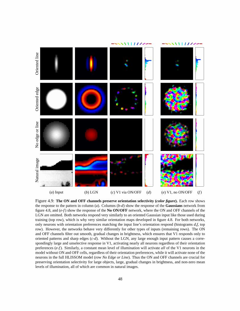
Orie

nted

line

Orie

nted

edge

No

edge

orlin

eN

atur

alim

age

(a) Input (b) LGN (c) V1 via ON/OFF (d) (e) V1, no ON/OFF (f )

Figure 4.9:The ON and OFF channels preserve orientation selectivity (color figure). Each row showsthe response to the pattern in column (a). Columns (b-d) show the response of theGaussiansnetwork fromfigure 4.8, and (e-f) show the response of theNo ON/OFF network, where the ON and OFF channels of theLGN are omitted. Both networks respond very similarly to an oriented Gaussian input like those used duringtraining (top row), which is why very similar orientation maps developed in figure 4.8. For both networks,only neurons with orientation preferences matching the input line’s orientation respond (histogramsd,f, toprow). However, the networks behave very differently for other types of inputs (remaining rows). The ONand OFF channels filter out smooth, gradual changes in brightness, which ensures that V1 responds only tooriented patterns and sharp edges (c-d). Without the LGN, any large enough input pattern causes a corre-spondingly large and unselective response in V1, activating nearly all neurons regardless of their orientationpreferences (e-f). Similarly, a constant mean level of illumination will activateall of the V1 neurons in themodel without ON and OFF cells, regardless of their orientation preferences, while it will activate none of theneurons in the full HLISSOM model (rowNo Edge or Line). Thus the ON and OFF channels are crucial forpreserving orientation selectivity for large objects, large, gradual changes in brightness, and non-zero meanlevels of illumination, all of which are common in natural images.

48

Chapter 5

Scaling HLISSOM simulations

In the previous chapter I introduced HLISSOM and showed how it can develop realistic maps oforientation preferences. So that the simulations would be practical to run, the maps covered onlyabout a 25mm2 area out of the full 2500mm2 area of human V1 (Wandell 1995). Yet despite thesmall area, each simulation required several hours of computer time and hundreds of megabytes ofmemory. Experiments with faces will require a much larger area of V1 and the visual field, becausemost tests with newborns use head-sized face patterns presented at a very close range. Such patternsfill up most of the newborn’s visual field. Other important phenomena also require large networks,including long-range contour integration, object recognition, and optic flow.

In this chapter I will introduce a set of scaling equations that I developed to make suchsimulations practical. Given a small-scale simulation, the equations make it possible to calculatethe parameter settings necessary to perform an equivalent but larger scale simulation. I will showthat the original and scaled simulations have similar function and map-level organization; the largermap just has more detail or a greater area, and takes more time and memory to simulate. Althoughthe equations are included here primarily because they will be used in later chapters, they are alsoan independent contribution that can be used with other incremental Hebbian models with architec-tures similar to RF-LISSOM or HLISSOM. As will be discussed below, the equations can also beapplied to biological systems, calculating how these systems differ in structure and thus how theirfunctions are likely to differ. Finally, the equations allow parameters for a model to be calculatedfrom measurements in animals of a particular species.

5.1 Background

Any particular HLISSOM or RF-LISSOM simulation models a fixed area of the visual field at afixed retinal density (receptors per visual field area) and a fixed cortical density (neurons per unit ofcortical area). Modeling new phenomena often requires using a different area or density. Changingthe area corresponds to modeling a larger portion of the visual space, e.g. a larger part of V1 and of

49

the eye. Changing the density corresponds to modeling a given area at a finer resolution (of eithercortical neurons or retinal receptors), as well as modeling a species, individual, or brain area thatdevotes more neurons or ganglia to the representation of a fixed amount of visual space.

Varying the area or density over a wide range is difficult in a complex nonlinear system likeHLISSOM. Parameter settings that work for one size will need to be very different to work properlywith other sizes. Furthermore, it is not always clear which parameters need to be adjusted at eachsize. To eliminate the search for appropriate parameters, I derived equations to compute the valuesneeded for each type of transformation. The equations treat any specific cortical network as a finiteapproximation to a continuous map composed of an infinite number of units. Similar continuousnetworks have been studied theoretically by Amari (1980) and Roque Da Silva Filho (1992). Undersuch an assumption, networks of different sizes represent coarser or denser approximations to thecontinuous map, and any given approximation can be transformed into another by (conceptually)reconstructing the continuous map and then resampling it. Given an existing retina and cortex ofsome fixed size, the scaling equations provide the parameter values needed for a smaller or largerretina and cortex to form a functionally equivalent map.

The following subsections will present the scaling equations for area, retinal ganglion den-sity, and cortical density, along with results from simulations of each type. The equations are alllinear, so they can also be applied together to change both area and density simultaneously. Ineach case, what the equations provide is a set of parameters for a new simulation that, when run,will develop similar results to the existing simulation. The equations are first derived on theoreticalgrounds, and then I verify experimentally that no other parameters need to be scaled, i.e. that theseparticular equations are sufficient.

5.2 Prerequisite: Insensitivity to initial conditions

One desirable property of a scaling algorithm is that it results in nearly identical final maps evensome parts of the network are changed, such as the retina size. Therefore, it is crucial that the maporganization not depend on the random initial weights, since those will vary between networks ofdifferent sizes. In this section I will show that the HLISSOM algorithm has exactly this property.

In HLISSOM, there are two types of variability between runs with different random num-bers: the random order, location, and position of the individual input patterns at each iteration,and the random initial values of the connection weights. Figure 5.1 demonstrates that the orienta-tion map shape does not depend on the random initial values of the weights, as long as the initialweights are drawn from the same random distribution. This result is surprising and significant, be-cause in many commonly used neural networks, the initial weights do play an important role (seee.g. Kolen and Pollack 1990).

Instead, the self-organized orientation map pattern in HLISSOM depends crucially on thestream of inputs, with two streams giving different orientation map patterns even if the streams are

50

Weight stream 1

Input stream 1

Weight stream 2

Input stream 1

Weight stream 2

Input stream 2

Initi

alm

ap

(a) (b) (c)

Ear

lym

ap

(d) (e) (f )

Fin

alm

ap

(g) (h) (i)

Figure 5.1:Input stream determines map pattern in HLISSOM (color figure). This figure shows thatthe self-organized orientation map patterns (e.g. in figure 4.7) do not depend on the random initial valuesof the weights. They are instead driven by the stream of input patterns presented during training. Using adifferent stream of random numbers for the weights results in different initial orientation maps (a andb),but has almost no effect on the final self-organized maps (compareg to h). In (g-i), the lateral inhibitoryconnections of one sample neuron are outlined in white, and are not affected by changing the weight stream.The final result is the same because lateral excitation smooths out differences in the initial weight values,and leads to similar large-scale patterns of activation at each iteration. (Compare mapsd ande measured atiteration 100; the same large-scale features are emerging in both maps despite locally different patterns ofnoise caused by the different initial weights.) In contrast, changing the input stream produces very differentearly and final map patterns (comparee to f andh to i), even when the initial weight patterns (and thereforethe initial orientation maps) are identical (b andc). Thus the input patterns are the crucial source of variation,not the initial weights.

51

drawn from the same distribution. The overall properties of the maps are very similar (number ofpinwheel centers, distance between them, etc.), but different input streams lead to different arrange-ments of blobs and pinwheel centers. In animals, maps are also similar between members of thesame species, but differ in the specific arrangements of blobs and pinwheel centers (Blasdel 1992b).Thus the HLISSOM model predicts that the specific orientation map pattern in the adult animaldepends primarily on the order and type of activity seen by the cortex in early development, and noton the details of the initial connectivity.

HLISSOM is insensitive to initial weights because of three features common to most otherincremental Hebbian models: (1) the scalar product input response function, (2) lateral excitationbetween neurons, and (3) the initial period with high learning rates. First, a neuron’s initial responseto an input pattern is determined by the sum of the product of each retinal receptor with its corre-sponding weight value (equation 4.6). For smoothly varying input patterns and large enough afferentRF size, this sum will have a very similar value regardless of the specific values of the weights toeach receptor. Thus, until the weights have self-organized into a smooth, spatially non-uniform dis-tribution, the input response of each neuron will be largely insensitive to the specific weight values.Second, settling due to lateral excitation (equation 4.7) causes nearby neurons to have similar finalactivity levels, which further reduces the contribution of each random afferent weight value. Third,Hebbian learning depends on the final settled activity levels resulting from an input (equation 4.8),and with a high enough learning rate, the initial weight values are soon overwritten by the responsesto the input patterns. As is clear in figure 5.1d,e, the large-scale map features develop similarly evenbefore the initial weight values have been overcome. Thus the Hebbian process of self-organizationis driven by the input patterns, not the initial weights.

The net result is that as long as the initial weights are generated from the same distribution,their precise values do not significantly affect map organization. Similar invariance to the initialweights should be found in other Hebbian models that compute the scalar product of the input anda weight vector, particularly if they include lateral excitation and use a high learning rate in thebeginning of self-organization. If a model does not have such invariance, scaling equations can stillgenerate functionally equivalent maps, but they will not be visually identical like the density-scaledmaps presented below.

5.3 Scaling equations

The following subsections will present the scaling equations for area, retinal ganglion density, andcortical density, along with results from simulations of each type.

5.3.1 Scaling the area

In this section I will consider the simplest case, changing the area of the visual space simulated.Scaling up the area allows a model to be developed quickly with a small area, then enlarged to

52

(a) Original cortexN = 54

0.4 hours, 8MB

(b) Cortex area scaledN = 4No = 4 · 54 = 216

9 hours, 148MB

(c) Original retinaR = 24

(d) Retina area scaledR = 4Ro = 4 · 24 = 96

Figure 5.2:Scaling the total area (color figure). Equations 5.1 can be used to scale the total area sim-ulated, in order to simulate a larger portion of the cortex, retina, and visual field. For largeN the numberof connections and the simulation time scale approximately linearly with the area, and thus a network fourtimes as wide and four times as tall (above) takes about sixteen times the memory and sixteen times as longto simulate. For discrete input patterns like these oriented Gaussians, larger areas require more input patternsto keep the total learning per neuron and per iteration constant. Because the inputs are generated randomlyacross the active surface of the retina, each map sees an entirely different stream of inputs, and so the finalmap patterns always differ when the area differs. The area scaling equations are most useful for testing amodel with a small area and then scaling up to eliminate border effects and to simulate the full area of acorresponding biological preparation.

eliminate border effects and to simulate the full area from a biological experiment. To change thearea, both the cortex widthN and the retina widthR must be scaled by the same proportionk

relative to their initial valuesNo andRo. (The ON and OFF channels of the LGN change just as theretina does, so their scaling equations are omitted below.)

What is perhaps less obvious is that, to ensure that the resulting network has the sameamount of learning per neuron per iteration, the average activity per input receptor needs to remainconstant. Otherwise a larger network would need to train for more iterations. Even if such longerlearning were not computationally expensive, changing the total number of iterations in HLISSOMhas non-linear effects on the outcome, because of the non-linear thresholding performed at eachiteration (equation 4.3). Thus when using discrete input patterns (rather than natural images), theaverage number of patternsı per iteration must be scaled with the retinal area. Consequently, theequations for scaling the area by a factork are:

N = kNo, R = kRo, ı = k2ıo (5.1)

See figure 5.2 for an example of scaling the retinal and cortical area.

53

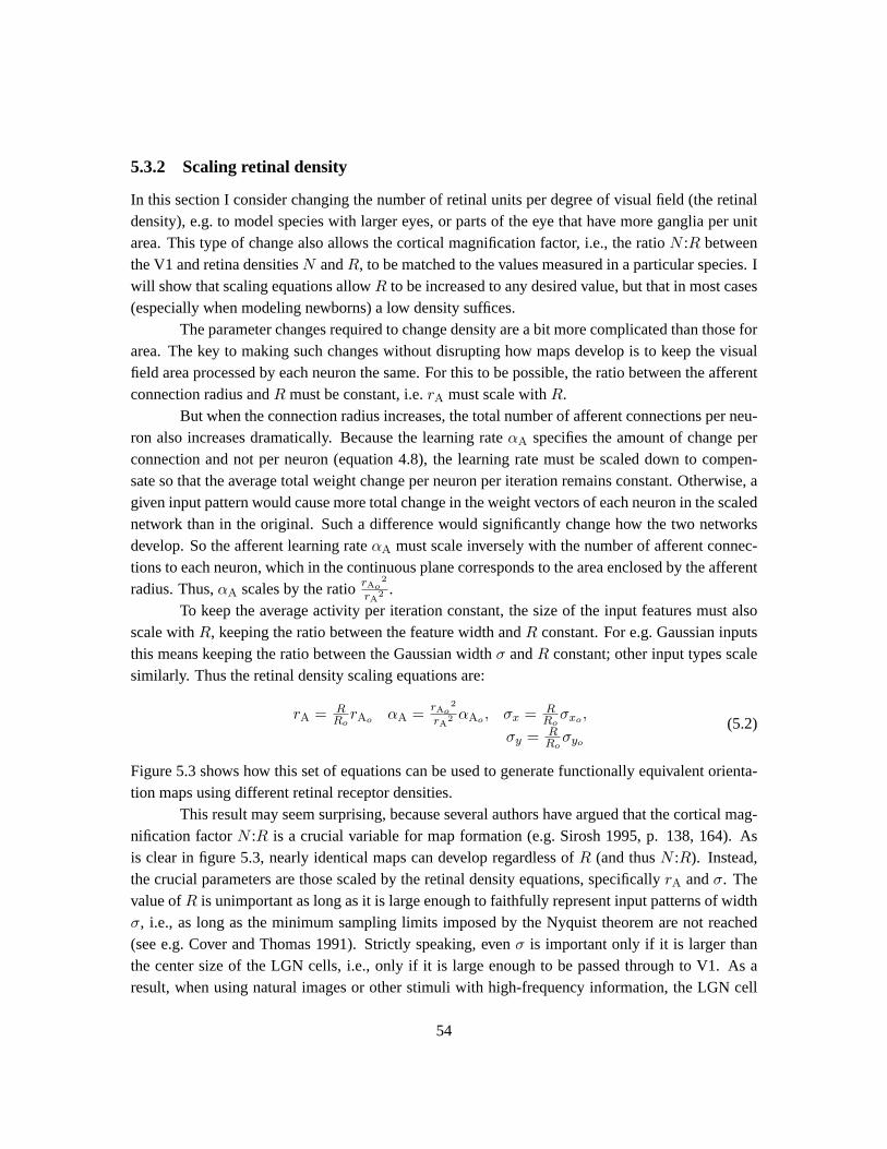
5.3.2 Scaling retinal density

In this section I consider changing the number of retinal units per degree of visual field (the retinaldensity), e.g. to model species with larger eyes, or parts of the eye that have more ganglia per unitarea. This type of change also allows the cortical magnification factor, i.e., the ratioN :R betweenthe V1 and retina densitiesN andR, to be matched to the values measured in a particular species. Iwill show that scaling equations allowR to be increased to any desired value, but that in most cases(especially when modeling newborns) a low density suffices.

The parameter changes required to change density are a bit more complicated than those forarea. The key to making such changes without disrupting how maps develop is to keep the visualfield area processed by each neuron the same. For this to be possible, the ratio between the afferentconnection radius andR must be constant, i.e.rA must scale withR.

But when the connection radius increases, the total number of afferent connections per neu-ron also increases dramatically. Because the learning rateαA specifies the amount of change perconnection and not per neuron (equation 4.8), the learning rate must be scaled down to compen-sate so that the average total weight change per neuron per iteration remains constant. Otherwise, agiven input pattern would cause more total change in the weight vectors of each neuron in the scalednetwork than in the original. Such a difference would significantly change how the two networksdevelop. So the afferent learning rateαA must scale inversely with the number of afferent connec-tions to each neuron, which in the continuous plane corresponds to the area enclosed by the afferentradius. Thus,αA scales by the ratiorAo

2

rA2 .

To keep the average activity per iteration constant, the size of the input features must alsoscale withR, keeping the ratio between the feature width andR constant. For e.g. Gaussian inputsthis means keeping the ratio between the Gaussian widthσ andR constant; other input types scalesimilarly. Thus the retinal density scaling equations are:

rA = RRo

rAo αA = rAo2

rA2 αAo , σx = R

Roσxo ,

σy = RRo

σyo

(5.2)

Figure 5.3 shows how this set of equations can be used to generate functionally equivalent orienta-tion maps using different retinal receptor densities.

This result may seem surprising, because several authors have argued that the cortical mag-nification factorN :R is a crucial variable for map formation (e.g. Sirosh 1995, p. 138, 164). Asis clear in figure 5.3, nearly identical maps can develop regardless ofR (and thusN :R). Instead,the crucial parameters are those scaled by the retinal density equations, specificallyrA andσ. Thevalue ofR is unimportant as long as it is large enough to faithfully represent input patterns of widthσ, i.e., as long as the minimum sampling limits imposed by the Nyquist theorem are not reached(see e.g. Cover and Thomas 1991). Strictly speaking, evenσ is important only if it is larger thanthe center size of the LGN cells, i.e., only if it is large enough to be passed through to V1. As aresult, when using natural images or other stimuli with high-frequency information, the LGN cell

54

(a) Original retinaR = 24, σx = 7, σy = 1.5

(b) V1 map forR = 24

(c) Retina scaled by 2.0R = 24 · 2 = 48, σx = 14, σy = 3

(d) V1 map forR = 48

(e) (e) Retina scaled by 3.0R = 24 ·3 = 72, σx = 21, σy = 4.5

(f ) V1 map forR = 72

Figure 5.3:Scaling retinal density (color figure). Equations (5.2) can be used to scale the density of retinalreceptors simulated per unit visual area, while keeping the area and the cortex density constant. This isuseful for matching the cortical magnification factor in a simulation, i.e., the ratio between the V1 and retinadensities, to the values from a particular species. Here each column shows an HLISSOM orientation mapfrom one of three matched 96×96 networks that have retinas of different densities. The parameters for eachnetwork were calculated using equations (5.2), and then each network was trained independently on the samerandom stream of input patterns. The size of the input pattern in retinal units increases as the retinal densityis increased, but its size as a proportion of the retina remains constant. All of the resulting maps are similaras long asR is large enough to represent the input faithfully, with almost no change aboveR = 48. Thus alow value can be used forR in practice.

RF size may instead be the limiting factor for map development. In practice, these results show thata modeler can simply use the smallestR that faithfully samples the input patterns, thereby savingcomputation time without significantly affecting map development.

55

(a) 36×360.17 hours, 2.0MB

(b) 48×480.32 hours, 5.2MB

(c) 72×720.77 hours, 22MB

(d) 96×961.73 hours, 65MB

(e) 144×1445.13 hours, 317MB

Figure 5.4:Scaling the cortical density (color figure). Five HLISSOM orientation maps from networksof different sizes are shown; the parameters for each network were calculated using equations (5.3), andthen each network was trained independently on the same random stream of input patterns. The size of thenetwork in the number of connections ranged from2 × 106 to 3 × 108 (2 megabytes to 317 megabytes ofmemory), and the simulation time ranged from ten minutes to five hours on the same machine, a single-processor 600MHz Pentium III. Simulations of 2048-megabyte192×192 networks on the massively parallelCray T3E supercomputer perform similarly. Despite this wide range of simulation scales, the final organizedmaps are both qualitatively and quantitatively similar, as long as their size is above a certain minimum (hereabout 64×64). Larger networks take significantly more memory and simulation time, but offer greater detailand will allow other dimensions such as ocular dominance and direction to be simulated in the same map.

5.3.3 Scaling cortical neuron density

Scaling the cortical density allows a small density to be used for most simulations, while making itpossible to scale up to the full density of the cortex to see details in the orientation maps. Scaling upis also important when simulating joint maps, such as combined ocular dominance, orientation, anddirection maps. Because of the numerous lateral connections within the cortex, the cortical densityhas the most effect on the computation time and memory, and thus it is important to choose theappropriate value needed for each simulation.

The equations for changing cortical density are analogous to those for retinal receptor den-sity, with the additional requirement that the intracortical connection sizes and associated learningrates must be scaled. The lateral connection radiirE andrI should be scaled withN so that theratio between each radius andN remains constant. For simulations that shrink the lateral excitatoryradius, the final radiusrEf

must also be scaled. LikeαA in retinal density scaling,αE andαI mustbe scaled so that the average total weight change per neuron per iteration remains constant despitechanges in the number of connections. Finally, the absolute weight levelDI below which lateralinhibitory connections are killed at a given iteration must be scaled when the total number of lateralconnections changes. The absolute value varies because the weight normalization in equation 4.8ensures that when there are fewer weights each one is stronger. The value of each weight is pro-portional to the number of connections, soDI should scale with the number of lateral inhibitoryconnections. In the continuous plane, that number is the area enclosed by the lateral inhibitoryradius. Thus, the cortical density scaling equations are:

56

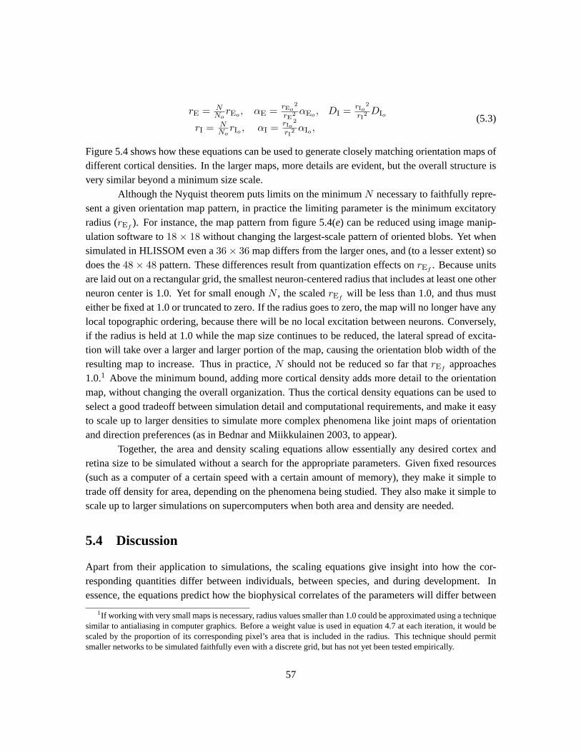
rE = NNo

rEo , αE = rEo2

rE2 αEo , DI = rIo

2

rI2 DIo

rI = NNo

rIo , αI = rIo2

rI2 αIo ,

(5.3)

Figure 5.4 shows how these equations can be used to generate closely matching orientation maps ofdifferent cortical densities. In the larger maps, more details are evident, but the overall structure isvery similar beyond a minimum size scale.

Although the Nyquist theorem puts limits on the minimumN necessary to faithfully repre-sent a given orientation map pattern, in practice the limiting parameter is the minimum excitatoryradius (rEf

). For instance, the map pattern from figure 5.4(e) can be reduced using image manip-ulation software to18 × 18 without changing the largest-scale pattern of oriented blobs. Yet whensimulated in HLISSOM even a36× 36 map differs from the larger ones, and (to a lesser extent) sodoes the48 × 48 pattern. These differences result from quantization effects onrEf

. Because unitsare laid out on a rectangular grid, the smallest neuron-centered radius that includes at least one otherneuron center is 1.0. Yet for small enoughN , the scaledrEf

will be less than 1.0, and thus musteither be fixed at 1.0 or truncated to zero. If the radius goes to zero, the map will no longer have anylocal topographic ordering, because there will be no local excitation between neurons. Conversely,if the radius is held at 1.0 while the map size continues to be reduced, the lateral spread of excita-tion will take over a larger and larger portion of the map, causing the orientation blob width of theresulting map to increase. Thus in practice,N should not be reduced so far thatrEf

approaches1.0.1 Above the minimum bound, adding more cortical density adds more detail to the orientationmap, without changing the overall organization. Thus the cortical density equations can be used toselect a good tradeoff between simulation detail and computational requirements, and make it easyto scale up to larger densities to simulate more complex phenomena like joint maps of orientationand direction preferences (as in Bednar and Miikkulainen 2003, to appear).

Together, the area and density scaling equations allow essentially any desired cortex andretina size to be simulated without a search for the appropriate parameters. Given fixed resources(such as a computer of a certain speed with a certain amount of memory), they make it simple totrade off density for area, depending on the phenomena being studied. They also make it simple toscale up to larger simulations on supercomputers when both area and density are needed.

5.4 Discussion

Apart from their application to simulations, the scaling equations give insight into how the cor-responding quantities differ between individuals, between species, and during development. Inessence, the equations predict how the biophysical correlates of the parameters will differ between

1If working with very small maps is necessary, radius values smaller than 1.0 could be approximated using a techniquesimilar to antialiasing in computer graphics. Before a weight value is used in equation 4.7 at each iteration, it would bescaled by the proportion of its corresponding pixel’s area that is included in the radius. This technique should permitsmaller networks to be simulated faithfully even with a discrete grid, but has not yet been tested empirically.

57

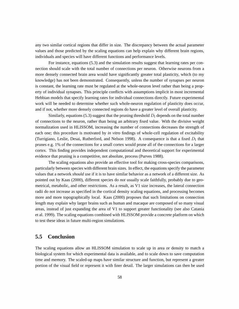
any two similar cortical regions that differ in size. The discrepancy between the actual parametervalues and those predicted by the scaling equations can help explain why different brain regions,individuals and species will have different functions and performance levels.

For instance, equations (5.3) and the simulation results suggest that learning rates per con-nection should scale with the total number of connections per neuron. Otherwise neurons from amore densely connected brain area would have significantly greater total plasticity, which (to myknowledge) has not been demonstrated. Consequently, unless the number of synapses per neuronis constant, the learning rate must be regulated at the whole-neuron level rather than being a prop-erty of individual synapses. This principle conflicts with assumptions implicit in most incrementalHebbian models that specify learning rates for individual connections directly. Future experimentalwork will be needed to determine whether such whole-neuron regulation of plasticity does occur,and if not, whether more densely connected regions do have a greater level of overall plasticity.

Similarly, equations (5.3) suggest that the pruning thresholdDI depends on the total numberof connections to the neuron, rather than being an arbitrary fixed value. With the divisive weightnormalization used in HLISSOM, increasing the number of connections decreases the strength ofeach one; this procedure is motivated byin vitro findings of whole-cell regulation of excitability(Turrigiano, Leslie, Desai, Rutherford, and Nelson 1998). A consequence is that a fixedDI thatprunes e.g. 1% of the connections for a small cortex would prune all of the connections for a largercortex. This finding provides independent computational and theoretical support for experimentalevidence that pruning is a competitive, not absolute, process (Purves 1988).

The scaling equations also provide an effective tool for making cross-species comparisons,particularly between species with different brain sizes. In effect, the equations specify the parametervalues that a networkshoulduse if it is to have similar behavior as a network of a different size. Aspointed out by Kaas (2000), different species donot usually scale faithfully, probably due to geo-metrical, metabolic, and other restrictions. As a result, as V1 size increases, the lateral connectionradii do not increase as specified in the cortical density scaling equations, and processing becomesmore and more topographically local. Kaas (2000) proposes that such limitations on connectionlength may explain why larger brains such as human and macaque are composed of so many visualareas, instead of just expanding the area of V1 to support greater functionality (see also Cataniaet al. 1999). The scaling equations combined with HLISSOM provide a concrete platform on whichto test these ideas in future multi-region simulations.

5.5 Conclusion

The scaling equations allow an HLISSOM simulation to scale up in area or density to match abiological system for which experimental data is available, and to scale down to save computationtime and memory. The scaled-up maps have similar structure and function, but represent a greaterportion of the visual field or represent it with finer detail. The larger simulations can then be used

58

to model large-scale phenomena that cannot be addressed in smaller models, such as joint maps ofmultiple stimulus features. Later chapters will use these equations to develop large-scale models ofV1 and show how they can be used as the first stage of a hierarchy of cortical regions.

59

Chapter 6

Development of Orientation Perception

This chapter will use the HLISSOM model and scaling equations introduced in the previous chap-ters to model orientation map development in detail, using realistic inputs. The results show thatboth internally generated and environmental stimuli are needed to explain the experimentally mea-sured orientation maps. Together these sources of activity can account for the complex process oforientation map development in V1. The simulations also act as a well-grounded test case for themethods used in the face perception experiments in later chapters.

6.1 Goals

In a series of simulations below, I will show that:

1. Orientation maps can develop from either random or structured (blob-like) internally gen-erated activity, but that structured activity is necessary for the maps to match experimentalmeasurements from newborn animals (section 6.2).

2. Orientation maps can also develop from natural images alone, and the distribution of orienta-tion preferences matches the distribution of orientations in those images (section 6.3).

3. Training on internally activity first, then natural images, shows how the orientation map canexist at birth, and then smoothly become a better match to the environment (section 6.4).

Thus either spontaneous activity or natural images alone would be sufficient to drive the develop-ment of orientation maps, but both together are required to explain the experimental data.

6.2 Internally generated activity

The simulations in chapter 4 used two-dimensional Gaussians as an idealized representation oforiented features in the input. This representation consists only of single short lines, uncorrelated

60

with each other or with the edges of larger objects. This section and the next will show how makingthe input patterns match more closely either to spontaneous activity or to natural images affectsthe final maps and RFs. So that these separate simulations can be compared to each other and toresults from other models, all of them will use the same type of input pattern throughout training,and all will use nearly identical conditions except for the specific input patterns. The goal of thesesimulations is to determine individually how each type of input affects development, so that it willbe clear how each contributes to the full model of prenatal and postnatal development that I willpresent in section 6.4.

First, I consider internally generated activity alone. As is clear from figure 1.1, a realisticmodel of patterns like the retinal waves would include large, coherent patterns of activity, as wellas background noise. Miller (1994) has argued that such patterns of activity are too large andtoo weakly oriented to drive the development of orientation preferences in V1. The results in thissection show that orientation selectivity and realistic maps can develop in HLISSOM even fromlarge, unoriented patterns of activity, and even with background noise. These results demonstratethat the known properties of retinal waves are sufficient for the development of orientation mapsand selectivity. Of course, many sources of internally generated activity other than retinal wavesmay also share these features, including PGO activity; the retinal waves are simply the best knownexample of such activity. Besides being sufficient, the results will show that training on the orientedblobs seen in retinal waves actually results in more realistic maps than generated by models that donot include such blobs, such as Miller’s.

6.2.1 Discs

To ensure that the internally generated blob patterns have no orientation bias, they were renderedfrom the following equations for a circular disc with smooth Gaussian falloff in brightness aroundthe edges. (The real patterns often do have orientation biases, but omitting them here shows that theelongated edges are not a necessary feature for orientation map development.) Each disc pattern isspecified by the location of the disc center(xi, yi), the widthw of the full-intensity central portionof the disc, and the half-widthσf for Gaussian smoothing of the outer border. To calculate theactivity for each photoreceptor(x, y), the Euclidean distanced of that photoreceptor from the disccenter is calculated:

d =√

(x− xi)2 + (y − yi)2. (6.1)

The activityξ for receptor(x, y) is then

ξx,y =

1.0 d < w2

exp(− (d−w2

)2

σf2 ) d >= w

2 .(6.2)

The x andy coordinates of the centers are each chosen randomly, and the orientation is chosenrandomly from the uniform distribution in the range 0◦ ≤ θ < 180◦. The brightness of each patternwas either positive or negative relative to the mean brightness, and was chosen randomly.

61

TheDiscsrow of figure 6.1 shows that even with input patterns that do not favor any partic-ular orientation, HLISSOM can develop oriented receptive fields with ON and OFF subregions, aswell as a realistic orientation map. As far as I am aware, this finding is the first demonstration thatorientation maps can develop from large, unoriented activity patterns. The development is drivenby the orientations of small patches around the edge of the circular discs. These oriented edges arevisible in the LGN response to the disc pattern in figure 6.1b. Because the input patterns had onlyedges and no lines or bars, most neurons develop two-lobed receptive fields, not three-lobed. Bothtwo-lobed and three-lobed receptive fields are common RF types for simple cells in adult V1 (Hubeland Wiesel 1968), but it is not known what RF types are present in newborns. These results suggestthat if orientation map development is driven by large, spatially coherent blobs of activity, newbornswill primarily have two-lobed receptive fields in V1.

6.2.2 Noisy Discs

The retinal waves in figure 1.1 contain spatially uncorrelated background noise in addition to theretinal waves. This noise is most likely a combination of measurement noise plus uncorrelatedneural activity. It is not clear how much noise is due to either source, but assuming at least some isdue to genuine neural activity is reasonable.

Here, I model the noise as a random additive value for each pixel, drawn from the uniformdistribution in the range±0.5. TheNoisy Discsrow in figure 6.1 shows that realistic maps developeven with substantial noise. However, the final map has fewer highly selective neurons. This resultsuggests that including the spatially uncorrelated noise may be important for faithfully modelingnewborn maps, which also tend to have lower selectivity.

6.2.3 Random noise

As a control, theRandom Noiserow in figure 6.1 shows that orientation maps can even developfrom uniformly random noise, where each input pixel is a random number between 0 and 1.0. Sucha simulation is in many respects similar to the simpler model of Linsker (1986a,b,c), who alsoshowed that orientation-selective neurons can develop from uncorrelated noise. Even such fullyrandom patterns have local clusters that are brighter or darker than their surround. These clusterslead to patches of activity in the ON channel adjacent to patches in the OFF channel (figure 6.1(b)).The result is that orientation-selective neurons develop even from uncorrelated noise. However,the resulting V1 map is less well organized than typically seen in animals, even at birth, and mostneurons develop much lower orientation selectivity than for the other patterns above. The lowerselectivity is particularly evident in the sample RFs, most of which would be a good match to manydifferent oriented lines.

These results show that even fully random activity can produce orientation maps, but suggestthat the inputs need to be spatially coherent for realistic RFs and maps to develop. Thus noise alone

62

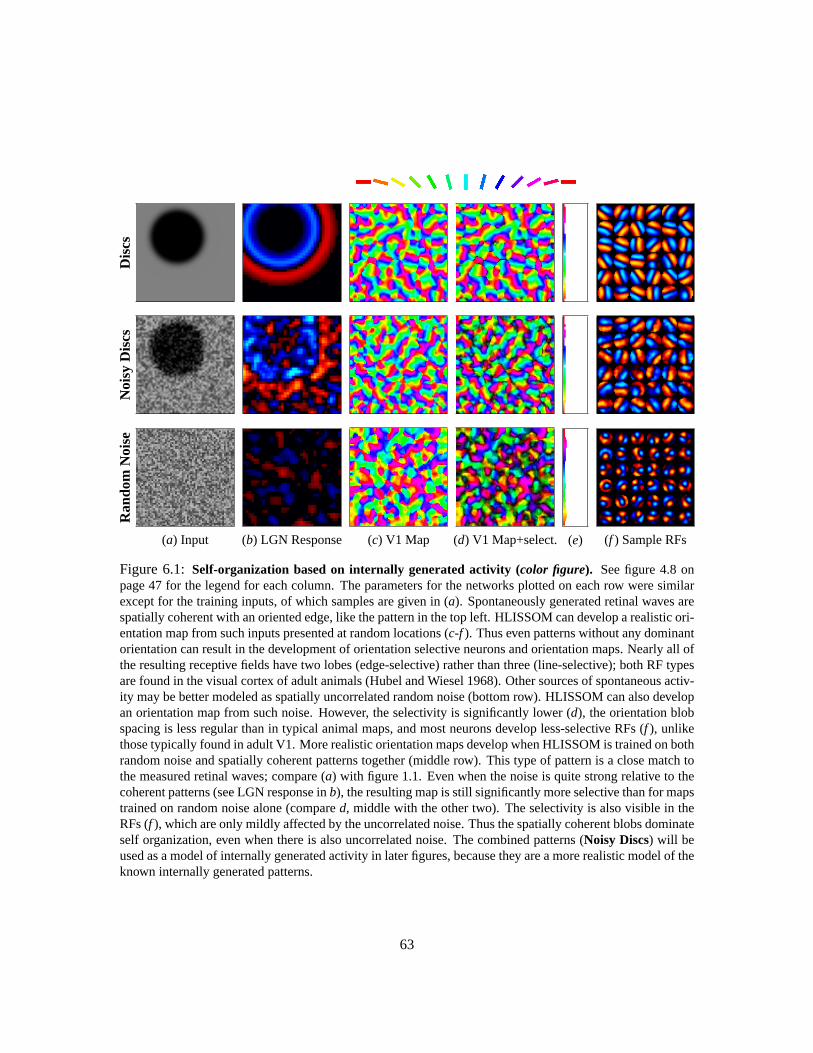
Dis

csN

oisy

Dis

csR

ando

mN

oise

(a) Input (b) LGN Response (c) V1 Map (d) V1 Map+select. (e) (f ) Sample RFs

Figure 6.1: Self-organization based on internally generated activity (color figure). See figure 4.8 onpage 47 for the legend for each column. The parameters for the networks plotted on each row were similarexcept for the training inputs, of which samples are given in (a). Spontaneously generated retinal waves arespatially coherent with an oriented edge, like the pattern in the top left. HLISSOM can develop a realistic ori-entation map from such inputs presented at random locations (c-f). Thus even patterns without any dominantorientation can result in the development of orientation selective neurons and orientation maps. Nearly all ofthe resulting receptive fields have two lobes (edge-selective) rather than three (line-selective); both RF typesare found in the visual cortex of adult animals (Hubel and Wiesel 1968). Other sources of spontaneous activ-ity may be better modeled as spatially uncorrelated random noise (bottom row). HLISSOM can also developan orientation map from such noise. However, the selectivity is significantly lower (d), the orientation blobspacing is less regular than in typical animal maps, and most neurons develop less-selective RFs (f ), unlikethose typically found in adult V1. More realistic orientation maps develop when HLISSOM is trained on bothrandom noise and spatially coherent patterns together (middle row). This type of pattern is a close match tothe measured retinal waves; compare (a) with figure 1.1. Even when the noise is quite strong relative to thecoherent patterns (see LGN response inb), the resulting map is still significantly more selective than for mapstrained on random noise alone (compared, middle with the other two). The selectivity is also visible in theRFs (f ), which are only mildly affected by the uncorrelated noise. Thus the spatially coherent blobs dominateself organization, even when there is also uncorrelated noise. The combined patterns (Noisy Discs) will beused as a model of internally generated activity in later figures, because they are a more realistic model of theknown internally generated patterns.

63

is insufficient. Of these simulations, theNoisy Discspatterns are both more realistic and developmaps that more closely match experimental results from newborn animals. I will therefore usethese patterns to model the prenatal phase of orientation map training in the combined prenatal andpostnatal model in section 6.4.

6.3 Natural images

Even though orientation maps are present at birth, how they develop postnatally depends on expe-rience with real images of the visual environment. This section and figure 6.2 show that HLISSOMcan realistic orientation maps and receptive fields from natural images, which has only been shownfor a few other models so far. Moreover, the distribution of orientation preferences that developsin HLISSOM depends on the statistical distribution of features in different sets of images. Suchdependence on the environment has been found for animal maps (Sengpiel et al. 1999), but to myknowledge has not yet been demonstrated in models.

To be comparable with the previous simulations of spontaneous activity and with othermodels using natural images, these simulations use natural images throughout the course of self-organization, and do not include a prenatal phase with spontaneous activity. Although the resultswill show that natural images alone would be sufficient to drive the development of orientationmaps, the simulations are not a close match to biology because they do not explain how the mapscould be present at birth. In section 6.4 I will combine natural images with internally generatedinputs to model the full process of prenatal and postnatal orientation map development, based onthese results from simpler conditions.

6.3.1 Image dataset: Nature

The Nature row of figure 6.2 shows the result from training an HLISSOM map on randomly se-lected36×36 patches of256×256-pixel natural images. The set of 25 images of naturally occurringobjects was taken by Shouval et al. (1997, 1996). The authors specifically excluded images withprominent straight lines, to show that such lines were not required for orientation selectivity to de-velop. Nearly all of these images are short-range closeups, although there are a few wide-anglelandscapes showing the horizon.

When trained on these images, the self-organized HLISSOM orientation map is quite similarto theDiscsandNoisy Discsmaps (compare theNature row of figure 6.2 with figure 6.1). Manyof the neurons have lower orientation selectivity than for the artificial stimuli, which is expectedbecause the natural images contain many patterns other than pure edges. Even so, most of the RFsare orientation selective, as found in V1 of animals.

Unlike in the networks trained on artificially generated stimuli, the distribution of orienta-tion preferences in the HLISSOMNature map is slightly biased towards horizontal and verticalorientations. This result suggests that the distribution of orientation preferences in both the model

64

Nat

ure

Land

scap

esF

aces

(a) Input (b) LGN Response (c) V1 Map (d) V1 Map+select. (e) (f ) Sample RFs

Figure 6.2:Orientation maps develop with natural images (color figure). See figure 4.8 for the legend foreach column. The networks plotted on each row were similar except for the set of training images used. Thenetwork in the top row was trained on images of natural objects and (primarily) close-range natural scenes,from Shouval et al. (1997, 1996). It develops a realistic orientation map, albeit with a lower selectivitythan for the artificial stimuli. The lower selectivity is unsurprising, because the natural stimuli have manyunoriented features. The map is slightly biased towards horizontal and vertical orientations (e), as is thenatural environment (Switkes et al. 1978). Other image databases with different distributions of orientedpatterns can have very different results. The second row shows results for a set of stock photographs fromthe National Park Service (1995), which are primarily landscapes with abundant horizontal contours. Theresulting map is dominated by neurons with horizontal orientation preferences (red), with a lesser peak forvertical orientations (cyan). Results with a database of upright human faces have the opposite pattern, witha strong peak at vertical and a lesser peak at horizontal (bottom row). Thus HLISSOM can self-organizeorientation maps and receptive fields from natural images, and the resulting maps reflect the statistics of theimage dataset. Later simulations combining natural inputs with internally generated patterns will show thatthis natural image learning can account for postnatal learning of contours in the environment.

65

and in animals reflects the over-representation of vertical and horizontal contours in the natural en-vironment (Switkes et al. 1978). The subsection below explores this dependence in more detail,because it illustrates why postnatal learning is important.

6.3.2 Effect of strongly biased image datasets: Landscapes and Faces

Raising animals in artificial environments that are biased towards certain orientations leads leads toa bias in the distribution of orientation-selective cells in V1 (Blakemore and Cooper 1970; Sengpielet al. 1999). To model being raised in different environments, albeit ones less extreme than in thosestudies, two networks similar to theNature map were trained on images of landscapes and faces,respectively. The landscapes images were a set of 58 stock photos from the National Park Service(1995). Nearly half of the images in this set are wide-angle photos showing the horizon or otherstrong horizontal contours; a few also include man-made objects such as fences. The face imagesare a set of 30 frontal photographs of upright human faces (Achermann 1995). The HLISSOM mapresulting from each image set is shown in theLandscapesandFacesrows of figure 6.2.

The Landscapesmap is strongly biased toward horizontal contours, with a much weakerbias for vertical. These biases are visible in the orientation map, which is dominated by red (hori-zontal) and, to a lesser extent, cyan (vertical). The opposite pattern of biases is found for theFacesmap, which is dominated by cyan (vertical), and to a lesser extent, red (horizontal). These diver-gent results replicate the single-unit results found in cats raised in skewed environments (Blakemoreand Cooper 1970). They also replicate the recent finding that such animals have orientation mapswith enlarged orientation domains for the orientations overrepresented in the environment (Seng-piel et al. 1999). Thus the HLISSOM model shows how different environments can influence thedevelopment of orientation maps. The result is that the most common contours in the environmentare the most well-represented in visual cortex.

6.4 Prenatal and postnatal development

The preceding simulations use only a single type of inputs (either artificial or images) throughouttraining, to show how each type of input affects development. This section shows that presentingthe most realistic internally generated pattern model (theNoisy Discs), followed by natural imagesrepresenting postnatal experience, can account for much of the prenatal and postnatal developmentof orientation selectivity.

Figure 6.3 demonstrates that (1) an initial map can be self-organized using prenatal patterns,(2) it can smoothly self-organize postnatally with natural images to improve selectivity, and (3) thepostnatal learning will closely match the properties of the map to the statistical properties of thenatural images. Interestingly, the early postnatal development of the HLISSOM map after iteration1000 was similar whether internally generated patterns or typical natural images were used. Thisresult replicates Crair et al.’s (1998) finding that normal visual experience typically has only a

66

Nat

ure

Land

scap

es

(a) 0: Initial map (b) 1000: End ofprenatal training

(c) 2500: Duringpostnatal training

(d) 10,000: End ofpostnatal training

Figure 6.3:Postnatal training makes orientation map match statistics of the environment (color figure).Each row shows results from a network trained for 1000 iterations on theNoisy Discspatterns from figure 6.1as a model of internally generated activity, then trained for 9000 further iterations using natural images tomodel postnatal visual experience. The orientation map plots (b-d) show selectivity as a brightness level,so that the postnatal improvement in selectivity will be visible. (a) and (b) are the same in each row. Thetop row shows the effect of postnatal training on theNature dataset. With these images, more neuronsbecome sensitive to horizontal and vertical contours, and the overall selectivity increases. However, theoverall map shape remains similar, as found in laboratory animals (Chapman et al. 1996; compare individualblobs between maps right to left or left to right). The postnatal changes when trained on theLandscapesdataset are similar but much more pronounced. With these images the network smoothly develops strongbiases for vertical and horizontal contours, within the pre-determined map shape. These results show thatpostnatal learning can gradually adapt the prenatally developed map to match the statistics of an animal’snatural environment, while explaining how a genetically specified orientation map can be present at birth.

small effect on map development in kittens, and that similar maps developed whether the eyes wereopen or closed. Yet atypical collections of natural images can cause readily visible changes in themap, which replicates findings from kittens raised with abnormal visual experience (Blakemore andCooper 1970; Sengpiel et al. 1999).

Figure 6.4 specifically compares the maps after prenatal and postnatal training to mapsmeasured at birth and adulthood in animals. The self-organized map is very similar to that found innewborn ferrets and binocularly deprived cats (Chapman et al. 1996; Crair et al. 1998), showing thateven simple internally generated inputs can account for the initial orientation map. The individual

67

(a) Prenatal map detail (b) Neonatal cat (1.9× 1.9mm)

(c) Adult map (d) Adult monkey (5× 5mm)

Figure 6.4: Prenatal and postnatal maps match animal data (color figure). After 1000 iterations ofprenatal training, theNature network from figure 6.3 has developed a rudimentary orientation map. Plot(a) shows the central30 × 30 region of this map, and plot (b) shows a map measured from a cat withoutprior visual experience. (Reprinted with permission from Crair et al. (1998), copyright 1998, AmericanAssociation for the Advancement of Science.) After postnatal training on natural images, the full96 × 96map is quite similar to measurements from experimental animals, including the monkey cortex shown here.(Reprinted with permission from Blasdel 1992b, copyright 1992 by the Society for Neuroscience). Thus theHLISSOM model explains both the prenatal and adult orientation maps found in experimental animals, asself-organization from internally generated and environmental stimuli.

68

0◦ 45◦ 90◦ 135◦ 180◦

(a) HLISSOM model

0◦ 45◦ 90◦ 135◦ 180◦

(b) Adult ferret

Figure 6.5:Orientation histogram matches experimental data.(a) Histogram of orientation preferencesfor theNature network from figure 6.4 and the top row of figure 6.3, which was trained first onNoisy Discsand then on theNature dataset. (b) Corresponding histogram for a typical adult ferret visual cortex (reprintedfrom Coppola et al. 1998; copyright National Academy of Sciences, U.S.A.; used with permission.) Bothadult ferrets and the HLISSOM model trained on natural images have more neurons representing horizontalor vertical than oblique contours, which reflects the statistics of the natural environment. HLISSOM mapstrained on internally generated patterns alone show an approximately flat distribution instead, because theywere shown an unbiased distribution of input patterns (round discs and/or random noise).

receptive fields that develop are also good approximations to simple cells in monkey and cat visualcortex (Hubel and Wiesel 1962, 1968). Finally, figure 6.5 shows that postnatal training on naturalimages causes the HLISSOM map to develop a bias for horizontal and vertical contours, and thatthe bias matches that found in orientation maps of adult ferrets (Chapman and Bonhoeffer 1998;Coppola et al. 1998). Thus HLISSOM can explain the animal results, and both phases are necessaryto account for the experimental data: internally generated patterns before birth, and experience withnatural images after birth.

6.5 Discussion

The results in this chapter show that prenatal training on internally generated activity, followedby postnatal training on natural images, can account for much of the development of orientationmaps, orientation selectivity, receptive fields, and lateral connections in V1. The same activity-dependent learning rules can explain development based on both types of neural activity, internallyand externally generated.

Both types of activity appear to serve important roles in this developmental process, and inparticular both are crucial for replicating the experimental data. Postnatal experience with environ-mental stimuli ensures that the map faithfully represents the environment, while prenatal develop-ment ensures that the map is functional even at eye opening. Prenatal development may also beimportant for the development of higher areas connected to V1 (e.g. V2 and V4), because it ensuresthat the map organization in V1 is approximately constant after birth (figure 6.3). As a result, the

69

higher areas can begin learning appropriate connection patterns with V1 even before eye opening.Comparing orientation maps and RFs trained on random noise versus those trained on im-

ages, discs, or Gaussians suggests that oriented features are needed for realistic RFs. Even thoughmaps can develop without such features, the RFs do not match those typically measured in animals.A similar result was recently found independently by Mayer, Herrmann, and Geisel (2001) usingsingle RF simulations. However, Mayer et al. (2001) conclude that natural images are required forrealistic RFs, because they did not consider patterns like theNoisy Discs. The results here suggestthat any pattern with large, coherent blobs of activity will suffice, and thus that natural images arenot strictly required for RF development.

In animals, the map present at eye opening is more noisy and and has fewer selective neuronsthan the prenatally trained maps shown in figures 6.3 and 6.4 (Chapman et al. 1996; Crair et al.1998). As a result, in animals the postnatal improvement in selectivity is larger than that shownhere for HLISSOM. The difference may result from the immature receptive fields in the developingLGN (Tavazoie and Reid 2000). Using a more realistic model of the developing LGN would resultin a larger postnatal improvement, but would make the model significantly more complex to analyze.Other factors that could contribute to the lower selectivity at birth include the greater variability ofcortical responses in infants, which will cause a lower apparent selectivity. Such behavior could bemodeled by adding internal noise to the prenatal neurons, which again would make the model morecomplex to analyze but could provide a closer match to the biological case.

A recent study has also reported that the distribution of orientation selective cells matchesthe environment even in very young ferrets, i.e. that horizontal and vertical orientations are over-represented in orientation maps at eye opening (Chapman and Bonhoeffer 1998). One possibleexplanation for these surprising results is the non-uniform distribution of retinal ganglia along thehorizontal and vertical meridians in the retina (Coppola et al. 1998), which could bias the statisticsof internally generated patterns. Regardless of such a prenatal bias, HLISSOM shows how visualexperience will also drive the map to develop preferences that match the visual environment.

6.6 Conclusion

Overall, the HLISSOM results show that internally generated activity and postnatal learning cantogether explain much of the development of orientation preferences. Either type of activity alonecan lead to orientation maps, but only with realistic prenatal activity and postnatal learning withreal images could the model account for the full range of experimental results. These studies alsoallowed the HLISSOM model to be tested and tuned in a domain that has abundant experimentaldata for validation, so that it can later be applied to other domains.

70

Chapter 7

Prenatal Development of Face Detection

In the previous chapter, I showed how internally generated patterns and visual experience can ex-plain prenatal and postnatal development of orientation preferences in V1, a relatively well-studiedarea. In this chapter and the next I will apply the same ideas to the development of face detection. Ifocus first on prenatal development, showing how internally generated activity can explain newbornface preferences. Chapter 8 will then model postnatal experience with real faces, and show that suchlearning can account for experimental results with older infants.

7.1 Goals

The prenatal face detection simulations in this chapter will demonstrate that:

1. A scaled-up HLISSOM model of V1 can extract the local orientations in large natural images,which means that it can be used as the first cortical stage in a hierarchical model of the visualsystem (section 7.2.1).

2. With this V1 map and internally generated activity, a higher level map can develop three-dotpreferences. This result shows that a hierarchy of brain areas can self-organize and functionat a detailed, realistic neural level (section 7.2.2).

3. Specific feature preferences at the different levels of the hierarchy can replicate the reportednewborn schematic pattern preferences, facelike and non-facelike (section 7.3.1).

4. Preferences for three-dot patterns result in significant preference for faces in natural images(section 7.3.2).

5. The shape of the internally generated patterns is important, but it does not need to be preciselycontrolled to result in face preferences (section 7.3.3).

71

Together, these results show that a system like the CONSPEC three-dot conceptual modelof face detection from Johnson and Morton (1991; described in section 3.3.5) can be implementedand tested computationally. Moreover, they provide a specific, plausible way that such a system forface detection could be constructed in the developing brain.

7.2 Experimental setup

As illustrated in figure 4.1 on page 35, newborn face detection experiments used multiple corticallevels, including both V1 and the FSA (face-selective area). They also included multiple inputregions, the photoreceptors and the PGO generating area.

Previous developmental models have been tested only for the small areas typical of thenetworks in chapters 4–6. However, the newborn face experiments that will be modeled in thischapter presented head-sized stimuli at a distance of about 20cm from the baby’s eyes. As a result,the stimuli filled a substantial portion of the visual field (about 45◦). To model behavior at thisscale, the scaling equations were used to scale up theDiscssimulation from figure 6.1 to model avery large V1 area (approximately 1600 mm2 total) at a relatively low sampling density per mm2

(approximately 50 neurons/mm2). The cortical density was first reduced to the minimum value thatwould show an orientation map that matches animal maps (36 × 36), and then the visual area wasscaled to be just large enough to cover the visual images to be tested (288× 288, i.e. width×8 andheight×8). The FSA size was less crucial, and was set arbitrarily at36× 36. The FSA RF size wasscaled to be large enough to span the central portion of a face.

The resulting network consisted of438 × 438 photoreceptors,220 × 220 PGO generatorunits,204× 204 ON-center LGN units,204× 204 OFF-center LGN units,288× 288 V1 units, and36× 36 FSA units, for a total of 408,000 distinct units. There were 80 million connections total inthe two cortical sheets, which required 300 megabytes of physical memory.

The RF centers of neurons in the FSA were mapped to the central160 × 160 region of V1such that even the units near the borders of the FSA had a complete set of afferent connectionson V1, with no FSA RF extending over the outside edges of V1. V1 was similarly mapped to thecentral192 × 192 region of the LGN channels, and the LGN channels to the central384 × 384region of the photoreceptors and the central192×192 region of the PGO generators.1 In the figuresin this chapter, only the area mapped directly to V1 will be shown, to ensure that all plots have thesame size scale. The input pattern size on the retina was based on measurements of the preferredspatial frequency of newborns, as cited by Valenza et al. (1996). That is, inputs were presented atthe spatial scale where the frequency most visible to newborns produced the largest V1 response inthe model. The remaining parameters are listed in section A.5.

1Note that the photoreceptors are modeled as having uniform density for simplicity; there is no increase in samplingdensity in the fovea.

72

7.2.1 Development of V1

V1 was self-organized for10, 000 iterations on 11 randomly located circular discs per iteration,each 50 units wide (figure 7.1a). These patterns were used for simplicity rather thanNoisy discsor a combination of discs and images, because the focus of these simulations is on the developmentof the higher-level FSA region. The background activity level was 0.5, and the brightness of eachdisc relative to this surround (either +0.3 or -0.3) was chosen randomly. The borders of each discwere smoothed into the background level following a Gaussian of half-widthσ = 1.5. After 10, 000iterations (10 hours on a 600MHz Pentium III workstation), the scaled-up map shown in figure 7.1eemerged. Figure 7.2 shows that this scaled-up model will extract the salient local orientations inlarge images, which has not yet been demonstrated for other models of V1 development.

7.2.2 Development of the FSA

After the V1 training, its weights were fixed to their self-organized values, and the FSA was allowedto activate and learn from the V1 responses. The FSA was self-organized for10, 000 iterationsusing two triples of circular dots per iteration, each arranged in a triangular face-like configuration(figure 7.3a). Each dot was 20 PGO units wide, and was 0.3 units darker than the surround, whichitself was 0.5 on a scale of 0 to 1.0. Each triple was placed at a random location whose center was atleast 118 PGO units away from the centers of others (to avoid overlap), with a random angle drawnfrom a narrow (σ = π/36 radians) normal distribution around vertical.

Because the face preferences found in newborns have all been for faces of approximatelythe same size (life-sized at a distance of around 20 cm), only a single training pattern size was used.As a result, the model will only be able to detect face-like patterns at one particular size scale. Ifresponse to multiple face sizes (i.e., distances) is desired, the spatial scale of the training patternscan be varied during self-organization (Sirosh and Miikkulainen 1996). However, the FSA in sucha simulation would need to be much larger to represent the different sizes, and the resulting patchyFSA responses would require more complex methods of analysis.

Using these three-dot patterns, the FSA was self-organized for10, 000 iterations (13 hourson a 600MHz Pentium III workstation). The result was the face-selective map shown in figure 7.3h,consisting of an array of neurons that respond most strongly to patterns similar to the trainingpatterns. Despite the overall similarities between neurons, the individual weight patterns are uniquebecause each neuron targets specific orientation blobs in V1. Such complicated patterns would bedifficult to specify and hardwire, but they arise naturally from internally generated activity.

As FSA training completed, the activation threshold (i.e.β in figure 4.5) was specificallyset to a high value, which ensures that only patterns that are a strong match to an FSA neuron’sweights will activate it. This way, the presence of FSA activity can be interpreted unambiguously asan indication that there is a face at the corresponding location in the retina, which will be importantfor measuring the face detection ability of the network.

73

(a) Generated pattern (b) LGN activity (c) V1 activity after training

(d) Afferent weights of one V1neuron

(e) Final V1 orientation map (f ) Detail of orientation map (e)

Figure 7.1:Large-scale orientation map training (color figure). These figures show a scaled-up versionof theDiscssimulation from figure 6.1, 8 times wider and 8 times taller. At this scale, the afferent weights ofeach neuron span only a small portion of the retina (d), and the orientation map has many more oriented blobstotal (e). Zooming in on the central36 × 36 portion (f ) of the288 × 288 map (e) shows that the underlyingstructure of the orientation map is similar to those in the previous chapter. The plot appears blockier, becausethe neuron density was reduced to the smallest acceptable value, so that the network would be practical tosimulate. Plot (c) shows that the orientation of each neuron that responds to the input is still a good match tothe orientation present at that retinal location, and thus that this network is a reasonable approximation to alarge area of V1 and the retina. Figure 7.2 will show similar results for this network using natural images.

The cortical maps were then tested on natural images and with the same schematic stimuli onwhich human newborns have been tested (Goren et al. 1975; Johnson and Morton 1991; Simion et al.1998b; Valenza et al. 1996). For all of the tests, the same set of model parameter settings describedin section A.5 were used. Schematic images were scaled to a brightness range (difference betweenthe darkest and lightest pixels in the image) of 1.0. Natural images were scaled to a brightness rangeof 2.5, so that facial features in images with faces would have a contrast comparable to that of the

74

(a) Sample visual image (b) LGN response (c) V1 response

Figure 7.2:Large-area orientation map activation (color figure). The scaled-up orientation map workswell with natural images; each V1 neuron responds if there is a line or edge of its preferred orientation at thecorresponding location in the retina. Because the V1 activations preserve the important features of the input,the output from V1 can be used as the input to a higher-level map. As suggested by figure 4.9, earlier modelslike RF-LISSOM will instead have a broad, unspecific response to natural images, even if they have realisticorientation maps.

schematic images. The different scales model different states of contrast adaptation mechanisms inthe retina that have not been implemented explicitly in this model.

7.2.3 Predicting behavioral responses

The HLISSOM model provides detailed neural responses for each neural region. These responsesconstitute predictions for future electrophysiological and imaging measurements in animals andhumans. However, the data currently available for infant face perception is behavioral. Specifically,it consists of newborn attention preferences measured from visual tracking distance and lookingtime. Thus, validating the model on this data will require predicting a behavioral response based onthe simulated neural responses.

As a general principle, I hypothesize that newborns pay attention to the stimulus whoseoverall neural response most clearly differs from typical stimuli. This idea can be quantified as

a(t) =F (t)F

+V (t)V

,+L(t)L

, (7.1)

wherea(t) is the attention level at timet, X(t) is the total activity in regionX at that time,X is theaverage (or median) activity of regionX over recent history, andF , V , andL represent the FSA,V1, and LGN regions, respectively. Because most stimuli activate the LGN and V1 but not the FSA,when a pattern evokes activity in the FSA newborns would attend to it more strongly. Yet stimulievoking only V1 activity could still be preferred over facelike patterns if their V1 activity is muchhigher than typical.

75

(a) Generated pattern (b) LGN activity (c) V1 activity before FSAtraining

(d) Afferent weights ofone FSA neuron

(e) FSA response beforetraining

(f ) FSA response aftertraining

(g) Initial map (h) Trained map

Figure 7.3:Training the FSA face map. (a) For training, the input consisted of simple three-dot configura-tions with random nearly vertical orientations presented at random locations in the PGO layer. These patternswere chosen based on the experiments of Johnson and Morton (1991). (b-c) The LGN and V1 sheets com-pute their responses based on this input. Initially, FSA neurons will respond to any activity in their receptivefields (e), but after training only neurons with closely matching RFs respond (f ). Through self-organization,the FSA neurons develop RFs (d) that are selective for a range of V1 activity patterns like those resultingfrom the three-dot stimuli. The RFs are patchy because the weights target specific orientation blobs in V1.This match between the FSA and the local self-organized pattern in V1 would be difficult to ensure withouttraining on internally generated patterns. Plots (g) and (h) show the afferent weights for every third neuronin the FSA. All neurons develop roughly similar weight profiles, differing primarily by the position of theirpreferred stimuli on the retina and by the specific orientation blobs targeted in V1. The largest differencesbetween RFs are along the outside border, where the neurons are less selective for three dot patterns. Overall,the FSA develops into a face detection map, signaling the location of facelike stimuli.

Unfortunately, such a formula is difficult to calculate in practice, because the order of pre-sentation of the stimuli in newborn experiments is not generally known. As a result, the average ormedian value of patterns in recent history is not available. Furthermore, the numerical preferencevalues computed in this way will differ depending on the specific set of patterns chosen, and thuswill be different for each study.

Instead, for the simulations below I will use a categorical approach inspired by Cohen (1998)that should yield similar results. Specifically, I will assume that when two stimuli both activate themodel FSA, the one with the higher total FSA activation will be preferred. Similarly, with two

76

stimuli activating only V1, the higher total V1 activation will be preferred. When one stimulusactivates only V1 and another activates both V1 and the FSA, I will assume that the newborn willprefer the pattern that produces FSA activity, unless the V1 activity is vastly greater than for typicalpatterns (as it is e.g. for a checkerboard pattern). Using these guidelines, the computed modelpreferences can be validated against the newborn’s looking preferences, to determine if the modelshows the same behavior as the newborn.

7.3 Face preferences after prenatal learning

This section presents the model’s response to schematic patterns and real images after it has com-pleted training on the internally generated patterns. The response to each schematic pattern is com-pared to behavioral results in infants, and the responses to real images constitute predictions forfuture experiments.

7.3.1 Schematic patterns

Figures 7.4 and 7.5 show that the model responses match the measured stimulus preference ofnewborns remarkably well, with the same relative ranking in each case where infants have showna significant preference between schematic patterns. These figures and the rankings are the mainresult from this simulation. I will next analyze each of the categories of preference rankings, toshow what parts of the model underlie the pattern preferences.

Most non-facelike patterns activate only V1, and thus the preferences between those patternsare based only on the V1 activity values (figure 7.4a,e-i; 7.5f -i). Patterns with numerous high-contrast edges have greater V1 response, which explains why newborns would prefer them. Thesepreferences are in accord with the simple LSM model, because they are based only on the earlyvisual processing (section 3.3.1).

Face-like schematic patterns activate the FSA, whether they are realistic or simply patternsof three dots (figure 7.4b-d; 7.5a-d). The different FSA activation levels reflect the level of V1response to each pattern, not the precise shape of the face pattern. Again the responses explain whynewborns would prefer patterns like the three-square-blob face over the oval-blob face, which hasa lower edge length. The preferences between these patterns are also compatible with the LSM,because in each case the V1 responses in the model match newborn preferences.

The comparisons between facelike and non-facelike patterns show how HLISSOM predic-tions differ from the LSM. HLISSOM predicts that the patterns that activate the FSA would bepreferred over those activating only V1, except when the V1 response is highly anomalous. MostV1 responses are very similar, and so the patterns with FSA activity should be preferred over mostof the other patterns, as found in infants. However, the checkerboard pattern (7.4a) has nearlythree times as much V1 activity as any other similar pattern. Thus HLISSOM explains why thecheckerboard would be preferred over other patterns, even ones that activate the FSA.

77

Ret

ina

LGN

V1

FS

A

2728

0.0

(a)

927

5.8

(b)

836

5.5

(c)

664

4.0

(d)

1094

0.0

(e)

994

0.0

(f )

931

0.0

(g)

807

0.0

(h)

275

0.0

(i)

Figure 7.4:Human newborn and model response to Goren et al.’s (1975) and Johnson et al.’s (1991)schematic images.TheRetina row along the top shows a set of patterns as they are drawn on the photore-ceptor sheet. These patterns have been presented to newborn human infants on head-shaped paddles movingat a short distance (about 20cm) from the newborn’s eyes, against a light-colored ceiling. In the experimentalstudies, the newborn’s preference was determined by measuring the average distance his or her eyes or headtracked each pattern, compared to other patterns. Below,x>y indicates that imagex was preferred overimagey under those conditions. Goren et al. (1975) measured infants between 3 and 27 minutes after birth.They found thatb>f>i andb>e>i. Similarly, Johnson et al. (1991), in one experiment measuring within onehour of birth, foundb>e>i. In another, measuring at an average of 43 minutes, they foundb>e, andb>h.Finally, Johnson and Morton (1991), measuring newborns an average of 21 hours old, found thata>(b,c,d),c>d, andb>d. The HLISSOM model has the same preference for each of these patterns, as shown in theimages above. The second row shows the model LGN activations (ON minus OFF) resulting from the pat-terns in the top row. The third row shows the V1 activations, with the numerical sum of the activities shownunderneath. If one unit were fully active, the sum would be 1.0; higher values indicate that more units areactive. The bottom row shows the settled response of the FSA. Activity at a given location in the FSA corre-sponds to a facelike stimulus at that location on the retina, and the sum of this activity is shown underneath.The images are sorted left to right according to the preferences of the model. The strongest V1 responseby nearly a factor of three is to the checkerboard pattern (a), which explains why the newborn would preferthat pattern over the others. The facelike patterns (b-d) are preferred over patterns (e-i) because of activationin the FSA. The details of the facelike patterns do not significantly affect the results — all of the facelikepatterns (b)–(d) lead to FSA activation, generally in proportion to their V1 activation levels. The remainingpatterns are ranked by their V1 activity alone, because they do not activate the FSA. In all conditions tested,the HLISSOM model shows behavior remarkably similar to that of the newborns, and provides a detailedcomputational explanation for why these behaviors occur.

78

Ret

ina

LGN

V1

FS

A

601

11.9

(a)

2081

11.8

(b)

2205

9.2

(c)

2154

8.3

(d)

2101

4.0

(e)

2244

0.0

(f )

2164

0.0

(g)

701

0.0

(h)

621

0.0

(i)

Figure 7.5:Response to schematic images from Valenza et al. (1996) and Simion et al. (1998a).Valenzaet al. measured preference between static, projected versions of pairs of the schematic images in the toprow, using newborns ranging from 24 to 155 hours after birth. They found the following preferences:d>f ,d>g, f>g, andh>i. Simion et al. similarly found a preference ford>g and b>e. The LGN, V1, andFSA responses of the model to these images are displayed here as in figure 7.4, and are again sorted by themodel’s preference. In all cases where the newborn showed a preference, the model preference matched it.For instance, the model FSA responds to the facelike pattern (d) but not to the inverted version (g). Patternsthat closely match the newborn’s preferred spatial frequencies (f ,h) caused a greater V1 response than theircorresponding lower-frequency patterns (g,i). Some non-facelike patterns with high-contrast borders cancause spurious FSA activation (e), because part of the border completes a three-dot pattern. Such spuriousresponses did not affect the predicted preferences, because they are smaller than the genuine responses.

Because the RFs in the model are only a rough match to the schematic patterns, the FSA canhave spurious responses to patterns that do not look like faces. For instance, the inverted three-dotpattern in Figure 7.5e activated the FSA, because part of the square outline filled in for the missingthird dot of an upright pattern. Figure 7.6 shows that such spurious responses should be expectedwith inverted patterns, even if neurons prefer upright patterns. This result may explain why somestudies have not found a significant difference between upright and inverted three-dot patterns (e.g.Johnson and Morton 1991). Because of the possibility of such spurious effects, future studies shouldinclude additional controls besides inverted three-dot patterns.

Interestingly, the model also showed a clear preference in one case where no significantpreference was found in newborns (Simion et al. 1998a): for the upright 3-blob pattern with no faceoutline (figure 7.5a), over the similar but inverted pattern (7.5i). The V1 responses to both patternsare similar, but only the upright pattern has an FSA response, and thus the model predicts that theupright pattern would be preferred.

79

Ret

ina

FS

AF

SA

-Hi

11.9

24.0

(a)

0.0

31.5

(b) (c) Upright (d) Inverted (e) Inverted symmetries

Figure 7.6:Spurious responses with inverted three-dot patterns.Several studies have used an invertedthree-dot pattern as a non-facelike control for an upright three-dot pattern (e.g. Johnson and Morton 1991;Simion et al. 1998a; Valenza et al. 1996). However, the results here show that this pattern does not make agood control, because of the many axes of symmetry of a three-dot pattern. These symmetries may explainwhy Johnson and Morton (1991) found no significant difference between the upright and inverted patterns,while Simion et al. (1998a) and Valenza et al. (1996) found that the upright pattern was preferred. TheFSArow above is the same as in figure 7.5, and shows that HLISSOM prefers the facelike upright pattern to thecontrol. However, the preference is sensitive to the value of the FSA thresholdδ and the FSA input scaleγA.For instance, ifγA is increased by 30%, the model FSA will respond more strongly to the inverted pattern(row FSA-Hi). As expected, the inverted pattern is not as good a match for any single neuron’s weights,so the blobs of FSA activity are always smaller for the inverted pattern. However, with a high enoughγA,the FSA responds in three different places (b), compared to only one for the upright pattern (a). These FSAresponses resemble an upright face pattern, but the resemblance is merely coincidental because the retinalstimulus was inverted. Together the three small responses outweigh the single larger response, assumingthat the total sum (and not the peak) activity is what determines preferences. Figure (e) shows that the threesmaller responses are due to matching any two out of the three possible blobs. In (e) I have marked the FSAresponses on top of the retinal pattern as three small dots. I have also drawn an outline around each of thepossible upright three-dot patterns that these responses represent. That is, each response represents one ofthe three overlapping upright patterns that share two dots with the inverted pattern. As shown in later figures,similar spurious responses can occur in real images when only one or two facial features are matched, ifother image features (such as parts of the face or hair outline) form a partial match for the missing features.For the other HLISSOM results with schematics, I setγA to a value low enough to prevent such spuriousresponses, which ensures that FSA neurons respond only to patterns that are a good match to their (upright)RFs. For humans, theγA value represents the state of contrast adaptation at a given time, which will varydepending on the recent history of patterns seen (cf. Albrecht et al. 1984; Turrigiano 1999). Thus these resultssuggest that infants will have no preference (or will prefer the inverted pattern) if they are tested on the high-contrast schematic patterns while being adapted to the lower contrast levels typical of the environment. Forinstance, an experimental protocol where there is a long time between schematic presentations could havesuch an effect. Because such adaptation is difficult to control in practice, the inverted pattern is a problematiccomparison pattern – negative results like those of Johnson and Morton (1991) may be due to temporarycontrast adaptation instead of genuine, long-term pattern preferences.

80

This potentially conflicting result may be due to postnatal learning rather than capabilitiesat birth. As will be shown in the next chapter, postnatal learning of face outlines can have a strongeffect on FSA responses. The newborns in the Simion et al. study were already 1–6 days old, and e.g.Pascalis et al. (1995) showed that newborns within this age range have already learned some of thefeatures of their mother’s face outline. Thus the HLISSOM model predicts that if younger newbornsare tested, they will show a preference for upright patterns even without a border. Alternatively,the border may satisfy some minimum requirement on size or complexity for patterns to attract anewborn’s interest. If so, the HLISSOM procedure for deriving a behavioral response from themodel response (section 7.2.3) would need to be modified to include such a constraint.

Overall, these results provide strong computational support for the speculation of Johnsonand Morton (1991) that the newborn could simply be responding to a three-dot face-like configura-tion, rather than performing sophisticated face detection. Internally generated patterns provide anaccount for how such “innate” machinery can be constructed during prenatal development.

7.3.2 Real face images

Most researchers testing newborns with schematic patterns assume that the responses to schematicsare representative of responses to real faces. However no experiment has yet tested that assumptionby comparing real faces to similar but non-facelike controls. HLISSOM makes testing real facespractical, which is an important way to determine the significance of the behavioral data. Theother model for newborn face preferences has not yet been tested with natural images (Acerra et al.2002), but the results reported here can be compared with future tests of that model. The examplesin figure 7.7 show that the prenatally trained HLISSOM model works remarkably well as a facedetector for natural images. The response is similar across a range of size scales and viewpoints,as shown in figure 7.8. This range is sufficient to account for typical newborn experiments, whichhave used a small range of size scales and only frontal views.

The face detection performance of the map was tested quantitatively using two image databases:a set of 150 images of 15 adult males without glasses, photographed at the same distance againstblank backgrounds (Achermann 1995), and a set of 58 non-face images of various natural scenes(National Park Service 1995). The face image set contained two views of each person facing for-wards, upwards, downwards, left, and right; figure 7.7a shows an example of a frontal view, andother views are shown in figure 7.8. Each natural scene was presented at 6 different size scales, fora total of 348 non-face presentations. Overall, the results indicated very high face detection perfor-mance: the FSA responded to 91% (137/150) of the face images, but to only 4.3% (15/348) of thenatural scenes.

Because the two sets of real images were not closely matched in terms of lighting, back-grounds, and distances, it is important to analyze the actual response patterns to be sure that thedifferences in the overall totals are genuine. The FSA responded with activation in the location cor-responding to the center of the face in 88% (132/150) of the face images. At the same time, the FSA

81

Ret

ina

LGN

V1

FS

A

4756

11.7

(a)

5778

7.5

(b)

6932

6.1

(c)

4797

11.1

(d)

4796

0.0

(e)

7614

0.0

(f )

7858

0.0

(g)

5072

0.0

(h)

4845

18.1

(i)

Figure 7.7:Model response to natural images.The top row shows a sample set of photographic images.The LGN, V1, and FSA responses of the model to these images are displayed as in figures 7.4 and 7.5. TheFSA is indeed activated at the correct location for most top-lit faces of the correct size and orientation (e.g.a-d). Image (a) is an example of one frontal view from the the Achermann (1995) database, which also includedthe other viewpoints shown in figure 7.8. For this database, 88% of the faces resulted in FSA activity in thecorrect location. Just as important, the network is not activated for most natural scenes (f -g) and man-madeobjects (h). For example, the FSA responded to only 4.3% of 348 presentations of landscapes and othernatural scenes from the National Park Service (1995). Besides human faces, the FSA responds to patternscausing a V1 response similar to that of a three-dot arrangement of contours (d,i), including related patternssuch as dog and monkey faces (not shown). Response is low to images where hair or glasses obscures theborders of the eyes, nose, or mouth, and to front-lit downward-looking faces, which have low V1 responsesfrom nose and mouth contours (e). The model predicts that newborns would show similar responses if tested.Credits: (a) copyright 1995 Bernard Achermann, (b-e) public domain; (f -i) copyright 1999-2001, James A.Bednar.

had spurious responses in 27% (40/150) of the face images, i.e. responses in locations other than thecenter of the face. Nearly half of the spurious responses were from the less-selective neurons thatline the outer border of the model FSA (see figure 7.3h); these responses can be ignored becausethey would be absent in a model of the entire visual field. Most of the remaining spurious responsesresulted from a genuine V1 eye or mouth response plus V1 responses to the hair or jaw outlines.If present in humans, such responses would actually serve to direct attention to the general regionof the face, and thus contribute to face preferences, although they would not pinpoint the precisecenter. For the natural scenes, most of the responses were from the less-selective neurons along theborder of the FSA, and those responses can again be ignored. The remainder were in image regionsthat coincidentally had a triangular arrangement of three contour-rich areas, surrounded by smooth

82

Ret

ina

LGN

V1

FS

A

4823

1.2

(a)

5275

13.7

(b)

4798

16.7

(c)

4626

15.2

(d)

4597

1.2

(e)

4427

18.4

(f )

4508

13.5

(g)

4478

12.7

(h)

4584

6.0

(i)

Figure 7.8:Variation in response with size and viewpoint.The three-dot training pattern of HLISSOMmatches most closely to a single size scale and an upright frontal view. However, it also responds to a rangeof other sizes (a-e). Here the responses of the model are again displayed as in figures 7.4-7.7. Newbornshave only been tested with a small range of sizes, and the range of patterns to which HLISSOM respondsis sufficient to explain those, even using a single-sized training pattern. The network is also insensitive tomoderate changes in viewpoint (f -i), responding in the correct FSA location to 88% of this set of 150 imagesconsisting equally of front, left, right, up, and down views. Most of these viewpoints give similar responses,with the biggest difference being that 100% of the faces looking upwards were detected correctly, but only80% of those looking downward were. Overall, HLISSOM predicts that newborns will respond to real faceseven with moderate variation of sizes and viewpoints, as long as they are lit from above like these images.

shading.

In summary, the FSA responds to most top-lit human faces of about the right size, signalingtheir location in the visual field. It does not respond to most other stimuli, except when they containaccidental three-dot patterns. The model predicts that human newborns will have a similar patternof responses in the face-selective cortical regions.

7.3.3 Effect of training pattern shape

The preceding sections show that a model trained on a triangular arrangement of three dots canaccount for face preferences at birth. This pattern was chosen based on Johnson and Morton’shypothesis that a hard-wired region responding to this pattern might explain newborn preferences.However, the actual shape of most internally generated activity in humans is unknown, and likeretinal waves, the shape may not be very precisely controlled in general. Thus it is important to testother possible training pattern shapes, to see what range of patterns can produce similar results.

83

Accordingly, I ran a series of simulations using a set of nine patterns that I chose to besimilar in overall size and shape to the three-dot patterns. The specific patterns are shown in theRetina row of figure 7.9. Matching the size is crucial to make the networks comparable, becauseonly a single sized training pattern is used in each network.

To make training and testing so many networks practical, I developed a simpler model with-out V1 that requires much less time and memory for each simulation (13 megabytes of memory and40 minutes of training time for self-organization). Without V1, the model does not provide numeri-cal preferences between the non-facelike patterns (i.e., those that activate V1 but not the FSA), butactivity in the FSA allows facelike patterns to be distinguished from other types, which is sufficientto measure the face selectivity of each network.

Specifically, the face selectivitySF was defined as the proportion of the average responseηF to a set of facelike patterns, out of the response to those patterns and the average responsesηN

to a set of non-facelike control patterns:

SF =∑

ηF∑ηF +

∑ηN

. (7.2)

A value of 1.0 indicates a strong preference for facelike patterns. It means that of the patterns tested,only the facelike patterns caused any FSA response. Values less than 0.5 indicate preference fornon-facelike schematics. To ensure that the comparisons between networks were fair, the sigmoidactivity threshold (δ in equation 4.4 on page 40) was set to maximize the face selectivity of eachnetwork. That is,δ was set to the minimum value for each network at which the FSA would respondto every facelike pattern. The upper threshold was then set toβ = δ +0.48, for consistency. If therewas no response to any non-facelike pattern with these settings,SF would be 1.0, the maximum.δ was set separately for schematics and real images, again to maximize the reported selectivity ofeach type.

Figure 7.9 shows that even with such a liberal definition of face selectivity, not all patternsresult in preferences for facelike schematics and real faces. Furthermore, several different patternsresult in high face selectivity. As expected, the results vary most strongly for schematic test images(row Schematics). The schematics are all closely matched for size, differing only by the patternswithin the face, and thus the results depend strongly on the specific training pattern. Of those result-ing in face selectivity, training patterns 7.9a-e (three dots, dots and bars, bars, and open triangles)have nearly equivalent selectivity, although the three dot pattern 7.9a has the highest.

The results were less variable on real test images, because real faces differ more from objectsthan the schematic faces differ from other schematic patterns. All training patterns that matchedeither the overall size of the test faces (7.9a-f ), or at least the eye spacing (7.9h-i), led to faceselectivity. In contrast, the single dot pattern (7.9g) does not lead to face preferences. Althoughit is a good match to the eyes and mouth regions in the real faces, it is also a good match to manyfeatures in object images. Thus even though most patterns that are matched for size will provide facepreferences under these conditions, general patterns like a single eye-sized dot are not sufficient.

84

Ret

ina

LGN

RF

Sch

emat

ics

Imag

es

1.0

1.0

(a)

0.9

1.0

(b)

0.9

1.0

(c)

0.8

1.0

(d)

0.8

0.8

(e)

0.6

0.7

(f )

0.5

0.4

(g)

0.3

0.9

(h)

0.3

1.0

(i)

Figure 7.9:Effect of the training pattern on face preferences.This figure shows results from nine matchedface detection simulations using easier-to-simulate networks without V1 (photoreceptors, LGN, and FSAonly). TheRetina row shows examples of the training patterns as they were drawn on the photoreceptorsin the first iteration of each simulation. At a given iteration, each simulation presented a different pattern atthe same locations and orientations. All other training parameters were also the same except for the FSA’sγA, which was set manually so that each simulation would have the same amount of activity per iterationof training, despite differences in the pattern sizes and shapes. TheLGN row shows the LGN response tothe retinal input, which forms the input to the FSA. TheRF row shows a sample FSA receptive field afterself-organization; other neurons learned similar RFs. In each case the HLISSOM network learns FSA RFssimilar to the LGN representation of the input patterns. Of course, the FSA RFs are no longer patchy, becausethey no longer represent the patchy V1 activities. The two numerical rows quantify the face selectivity ofeach network. TheSchematics row shows the selectivity for facelike schematics (figure 7.4b-d) relative tonon-facelike schematics (figure 7.4e-i). TheImages row shows the selectivity for the six face images fromfigure 8.2 on page 90, relative to the six comparable object images in the same figure. The results showthat different training patterns gave rise to different selectivities. Pattern (g) leads to equal responses forboth facelike and non-facelike schematics (selectivity of 0.5), and (h-i) have a greater overall response to thenon-facelike schematics (selectivity lower than 0.5). Thus not all training patterns are sufficient to explainpreferences for schematic faces, even if they match some parts of the face. Similarly, the single dot pattern(g) has a selectivity below 0.5 for real faces, indicating a stronger response for the objects than for real faces.The other training patterns are all matched either for size with the real faces, or match at least two parts of theface, and thus have face selectivities larger than 0.5 for real images. Overall, the shape of the training patternis clearly important for face selectivity, both for schematics and real faces, but it need not be controlled verytightly to result in face-selective responses.

85

Overall, these results show that matching the large-scale pattern size provides selectivity forfaces. Further matching the pattern shape provides further selectivity, which can be tested with theschematic patterns. Of all training patterns tested, the three-dot pattern provides the most selec-tivity, while simply matching a single low-level feature like eye size is not enough to provide facepreferences. Because of its high face selectivity, the three-dot pattern is a good default choice forpattern generation simulations, so that the predictions will most clearly differ from those of othermodels.

7.4 Discussion

The HLISSOM simulations show that internally generated patterns and self-organization can to-gether account for newborn face detection. Importantly, predictions from the HLISSOM modeldiffer from those of other recent models of newborn face preferences. These predictions can betested by future experiments.

One easily tested prediction of HLISSOM is that newborn face preferences should not de-pend on the precise shape of the face outline. The Acerra et al. (2002) model (section 3.3.2) makesthe opposite prediction, because in that model preferences arise from precise spacing differencesbetween the external border and the internal facial features. HLISSOM also predicts that newbornswill have a strong preference for real faces (e.g. in photographs), while I argue that the Acerra et al.model predicts only a weak preference for real faces, if any.

Experimental evidence to date cannot yet decide between the predictions of these two mod-els. For instance, Simion et al. (1998a) did not find a significant schematic face preference innewborns 1–6 days old without a contour surrounding the internal features, which is consistent withthe Acerra et al. model. However, the same study concluded that the shape of the contour “did notseem to affect the preference” for the patterns, which would not be consistent with the Acerra et al.model. As discussed earlier, younger newborns may not require any external contour, as HLISSOMpredicts, until they have had postnatal experience with faces. Future experiments with younger new-borns should compare model and newborn preferences between schematic patterns with a variety ofborder shapes and spacings. These experiments will either show that the border shape is crucial, aspredicted by Acerra et al., or that it is unimportant, as predicted by HLISSOM.

The HLISSOM model also makes predictions that differ from those of the Simion et al.(2001) “top-heavy” model (reviewed in section 3.3.3). The top-heavy model predicts that any face-sized border that encloses objects denser at the top than the bottom will be preferred over similarschematic patterns. HLISSOM predicts instead that a pattern with three dots in the typical symmet-rical arrangement would be preferred over the same pattern with both eye dots pushed to one side,despite both patterns being equally top-heavy. These two models represent very different explana-tions of the existing data, and thus testing such patterns should offer clear support for one modelover the other.

86

On the other hand, many of the predictions of the fully trained HLISSOM model are similarto those of the hardwired CONSPEC model proposed by Johnson and Morton (1991). In fact,the reduced HLISSOM face preference network in section 7.3.3 (which does not include V1) canbe seen as the first CONSPEC system to be implemented computationally, along with a concreteproposal for how such a system could be constructed during prenatal development (Bednar andMiikkulainen 2000a). The primary functional difference between the trained HLISSOM networkand CONSPEC is that only cortical regions contain face-selective neurons in HLISSOM. Whethernewborn face detection is mediated cortically or subcortically has been debated extensively, yet noclear consensus has emerged from behavioral studies (Simion et al. 1998a). If future brain imagingstudies do discover face-selective neurons in subcortical areas in newborns, HLISSOM will needto be modified to include such areas. Yet the key principles would remain the same, because thesubcortical regions may also be organized from internally generated activity. Thus experimentaltests of HLISSOM vs. CONSPEC should focus on how the initial system is constructed, and notwhere it is located.

7.5 Conclusion

Internally generated patterns explain how genetic influences can interact with general adaptationmechanisms to specify and develop newborn face processing circuitry. The HLISSOM model of thevisual system incorporates this idea, and is the first to self-organize both low-level and high-levelcortical regions at the scale and detail needed to model such behavior realistically. The results matchexperimental data from newborns remarkably well, and for the first time demonstrate preferencesfor faces in real images. Chapter 8 will show that the prenatally trained map can learn from realimages after birth, and that such learning can explain how face processing develops postnatally.

87

Chapter 8

Postnatal Development of Face Detection

As shown in the previous chapter, prenatal learning of internally generated patterns can lead to facepreferences at birth. In this chapter I show that the prenatally trained system can learn from faces inreal images. This learning process suggests novel explanations for experimental phenomena, suchas the disappearance of schematic face preferences, and provides concrete predictions for futurebehavioral experiments. Together, the face processing simulations show that learning of activitypatterns can explain how face preferences develop prenatally and postnatally in young infants.

8.1 Goals

The postnatal face detection simulations in this chapter will demonstrate that:

1. Prenatal training leads to faster and more robust learning after birth, compared to a systemexposed only to environmental stimuli (section 8.3.1).

2. The decline in infants’ response to schematic patterns in the periphery after one month maysimply result from learning real faces, not from a shift to a separate system (section 8.3.2).

3. Learning of both facial features and outlines, holistically, can explain the development of amother preference, including why it disappears when the outline is masked (section 8.3.3).

These simulations focus on peripheral vision, which is what most tests of newborn and young infantface preferences measure (Johnson and Morton 1991). However, as discussed in section 8.4, similarmechanisms can also explain the later development of face preferences in central vision. The resultssuggest that the delay in central vision is simply due to postnatal development of the retina, againwithout a shift to a separate cortical subsystem.

88

8.2 Experimental setup

Postnatal experiments in newborns have tested only basic face selectivity, not detailed preferencesbetween patterns of different spatial frequencies like in the newborn tests. As a result, the reducedHLISSOM model (without V1) is sufficient to model postnatal learning. Using the reduced modelmakes it practical to simulate much larger FSA RFs, which will be crucial for simulating postnatalface outline learning. For these experiments, the model was first trained “prenatally” as shown infigure 7.9a on page 85.

8.2.1 Control condition for prenatal learning

To determine whether the prenatal patterns bias subsequent learning (goal 1 above), a control net-work was also simulated, without prenatally organized receptive fields. This control will be calledthe naıve network, because it models neurons that have not had experience with coherent activitypatterns until after birth. The intent is to see if neurons that are initially face selective, due to pre-natal training on internally generated patterns, will learn faces more robustly than neurons that areinitially unselective and learn only from the environment postnatally.

So that the naıve and prenatally organized networks would match on as many parameters aspossible, I constructed the naıve network from the prenatally trained networkpost hocby explicitlyresetting afferent receptive fields to their uniform-Gaussian starting point. This procedure removedthe prenatally developed face selectivity, but kept the lateral weights and all of the associated pa-rameters the same. The activation thresholdδ for the naıve FSA network was then adjusted so thatboth networks would have similar activation levels in response to the training patterns; otherwisethe parameters were the same for each network. This procedure ensures that the comparison be-tween the two networks will be as fair as possible, because the networks differ only by whether theneurons have face-selective weights at birth. Figure 8.1 shows the state of each network just beforepostnatal learning.

8.2.2 Postnatal learning

The experiments in this chapter simulate gradual learning from repeated encounters of specific in-dividuals and objects against different backgrounds, over the first few months of life. Figure 8.2shows the people and objects that were used and figure 8.3 describes how the training images weregenerated. The prenatally trained and naıve networks were each exposed to the same random se-quence of 30,000 images, so that the influence of prenatal training on postnatal learning will beclear.

The RF changes in these simulations over time were larger than in the postnatal learningexperiments in chapter 6, because the weights were initially concentrated only in the center (fig-ure 8.1). As the weights spread out over the receptive field, the strength of the neural responses totypical training inputs varied significantly. To compensate for these changes, I periodically adjusted

89

(a) Prenatally trained network (b) Naıve network

Figure 8.1:Starting points for postnatal learning. These plots show the RFs for every third neuron fromthe24 × 24 array of neurons in the FSA. For the prenatally trained network (a), the RFs were visualized bysubtracting the OFF weights from the ON. The result is a plot of the retinal stimulus that would most excitethat neuron. As in chapter 7, the prenatally trained network consists of an array of roughly facelike RFs. Incontrast, the neurons in the naıve network are initially uniformly Gaussian. The ON and OFF weights wereidentical, so only the ON weights are shown in (b). Later figures will compare the postnatal learning of eachnetwork.

Figure 8.2:Postnatal learning source images.Simulations of postnatal learning used the above person andobject images (person images adapted from Rowley et al. 1998; objects are from public domain clip art andimage collections.) As shown in figure 8.3, each of these items was presented at random locations in front ofrandomly chosen natural scenes.

90

Ret

ina

LGN

FS

A

(a) (b) (c) (d) (e) (f )

Figure 8.3: Sample postnatal learning iterations. The top row shows six randomly generated imagesdrawn on the retinal photoreceptors at different iterations. Each image contains a foreground item chosenrandomly from the images in figure 8.2. The foreground item was overlaid onto a random portion of animage from a database of 58 natural scenes (National Park Service 1995), at a random location and at anearly vertical orientation (drawn from a normal distribution around vertical, withσ = π/36). The secondrow shows the LGN response to each of these sample patterns. The bottom row shows the FSA responseto each pattern at the start of postnatal training. For the FSA, only neurons with complete receptive fields(those in the unshaded inner box) were simulated, because those in the gray area would have RFs cut offby the edge of the retina. The gray area shows the FSA area that corresponds to the same portion of thevisual field as in the LGN and retina plots; with this representation, points in the FSA are mapped directlyto the corresponding location in the LGN and retina. At the start of postnatal training, the FSA responds togroups of dark spots on the retina, such as the eyes and mouths in (b-c,f) and the horse’s dark markings in(d); the location of the FSA activity corresponds to the position of the group of retinal patterns that caused theresponse. Subsequent learning in the FSA will be driven by these patterns of activity. The prenatal trainingbiases the activity patterns towards faces, and so postnatal self-organization will also be biased towards faces.

the sigmoid thresholdδ from equation 4.4 for each network. Without such compensation, the net-works eventually fail to respond to any training input, because the fixed total amount of weights hasbecome spread out over a much larger area than initially. The specific parameter values are listed insection A.4. Chapter 9 will discuss how this process can be simplified by extending HLISSOM withautomatic mechanisms for setting the threshold based on the recent history of inputs and responses,as found in many biological systems (Turrigiano 1999).

91

8.2.3 Testing preferences

In the previous chapter, pattern preferences were measured in a fully organized network that hadsimilar RFs across the visual field. With such a uniform architecture, image presentations generallyobtained similar responses at different retinal locations. In this chapter, the network pattern prefer-ences will be measured periodically during early postnatal learning, before the network has becomefully uniform.

To allow clear comparisons in this more-variable case, preferences will be measured hereby presenting input stimuli at 25 different retinal locations, averaging the results, and computingthe statistical significance of the difference between the two distributions. All comparisons will usethe Student’s t-test, with the null hypothesis being that the network responds equally strongly toboth stimuli. To match the psychological experiments, I will consider a calculatedp ≤ 0.05 to beevidence of a significant difference between responses to the two stimuli.

8.3 Results

8.3.1 Bias from prenatal learning

Figure 8.4 shows that with postnatal exposure to real images, both the naıve and prenatally trainednetworks develop RFs that are averages (i.e. prototypes) of faces and hair outlines. RFs in theprenatally trained network gradually become more face-selective, and eventually nearly all neuronsbecome highly selective (figure 8.4b).

Postnatal self-organization in the naıve network is less regular, and the final result is oftenless face selective. For example, the postnatal network often develops neurons selective for theclock. The clock has a high-contrast border that is a reasonably close match to real face outlines,and thus the same naıve network neurons tend to respond to both the clock and to real faces duringtraining. But the clock is a very weak match to the three-dot training pattern in the prenatally trainednetwork, and so that network rarely develops clock-selective neurons. These results suggest that theprenatal training biases postnatal learning towards biologically relevant stimuli, i.e. faces.

8.3.2 Decline in response to schematics

Figure 8.5 shows that the HLISSOM model replicates the disappearance of peripheral schematicface preferences after one month (Johnson et al. 1991). In HLISSOM, the decrease results from theafferent weight normalization (equation 4.8). As the FSA neurons in HLISSOM learn the hair andface outlines typically associated with real faces, the connections to the internal features necessarilybecome weaker. Unlike real faces, the facelike schematic patterns match only on these internalfeatures, not the outlines. As a result, the response to schematic facelike patterns decreases as realfaces are learned. Eventually, the response to the schematic patterns approaches and drops belowthe fixed activation threshold (δ in equation 4.4). At that point, the model response is no longer

92

(a) Prenatally trained network

0 6,000 10,000 12,000 16,000 20,000 30,000

(b) Snapshots of typical prenatally trained RFs

(c) Naıve network

0 6,000 10,000 12,000 16,000 20,000 30,000

(d) Snapshots of naıve network RFs

Figure 8.4:Prenatal patterns bias postnatal learning in the FSA.Plots (a) and (c) show the final RFs forevery third neuron from the24× 24 array of neurons in the FSA, visualized as in figure 8.1(a). As the prena-tally trained network learns from real images, the RFs morph smoothly into prototypes, i.e. representationsof average facial features and hair outlines (b). By postnatal iteration 30,000, nearly all neurons have learnedface-like RFs, with very little effect from the background patterns or non-face objects (a). Postnatal learningis less uniform for the naıve network, as can be seen in the RF snapshots in (d). In the end, many of the naıveneurons do learn face-like RFs, but others become selective for general texture patterns, and some becomeselective for objects like the clock (c). Overall, the prenatally trained network is biased towards learningfaces, while the initially uniform network more faithfully represents the environment. Thus prenatal learningcan allow the genome to guide development in a biologically relevant direction.

93

Ret

ina

LGN

FS

A-0

FS

A-1

000

(a) (b) (c) (d) (e) (f )

Figure 8.5:Decline in response to schematic faces.Before postnatal training, the prenatally trained FSA(third row from top) responds significantly more to the facelike stimulus (a) than to the three-dot stimulus (b;p = 0.05) or the scrambled faces (c-d; p = 10−8). Assuming that infants attend most strongly to the stimulithat cause the greatest neural response, these responses replicate the schematic face preferences found byJohnson and Morton (1991) in infants up to one month of age. Some of the Johnson and Morton 1991experiments found no significant difference between (a) and (b), which is unsurprising given that they areonly barely significantly different here. As the FSA neurons learn from real faces postnatally, they respondless and less to schematic faces. The bottom row shows the FSA response after 1000 postnatal iterations.The FSA now rarely responds to (a) and (b), and the average difference between them is no longer significant(p = 0.25). Thus no preference would be expected for the facelike schematic after postnatal learning, whichis what Johnson and Morton (1991) found for older infants, i.e. 6 weeks to 5 months old. The response to realfaces also decreases slightly through learning, but to a much lesser extent (e-f). The response to real facesdeclines because the newly learned average face and hair outline RFs are a weaker match to any particularface than were the original three dot RFs. That is, the external features vary more between individuals than dothe internal features, as can be seen in figure 8.2, and thus their average is not a close match to any particularface. Even so, there is only a comparatively small decrease in response to real faces, because real faces arestill more similar to each other than to the schematic faces. Thus HLISSOM predicts that older infants willstill show a face preference if tested with more-realistic stimuli, such as photographs.

94

higher for schematic faces (because there is no FSA response, and V1 responses are similar). In asense, the FSA has learned that real faces typically have both innerandouter features, and does notrespond when either type of feature is absent or a poor match to real faces.

Yet the FSA neurons continue to respond to real faces (as opposed to schematics) throughoutpostnatal learning (figure 8.5e-f). Thus the model provides a clear prediction that the decline inperipheral face preferences is limited to schematics, and that if infants are tested with sufficientlyrealistic face stimuli, no decline in preferences will be found.

This prediction is an important difference from the CONSPEC/CONLERN model, wherethe decline was explained as an effect of CONLERN maturing and beginning to inhibit CONSPEC.CONSPEC/CONLERN predicts that the decline in preferences for schematic faces also representsa decline in preference for real faces. HLISSOM predicts instead that an initially CONSPEC-likesystem is also like CONLERN, in that it will gradually learn from real faces. These divergentpredictions can be tested by presenting real faces in the periphery to infants older than one month;HLISSOM predicts that the infant will prefer the real face to other non-facelike stimuli.

8.3.3 Mother preferences

Figure 8.6a-b shows that when one face (i.e. the mother) appears most often, the FSA response tothat face becomes significantly stronger than to a similar stranger. This result replicates the motherpreference found in infants a few days old (Bushnell 2001; Pascalis et al. 1995; Walton and Bower1993; Walton, Armstrong, and Bower 1997; Bushnell et al. 1989).

Interestingly, figure 8.6c-d shows that the mother preference disappears when the hair out-line is masked, which is consistent with Pascalis et al.’s claim that newborns learn outlines only.However, Pascalis et al. (1995) did not test the crucial converse condition, i.e. whether newbornsrespond when the facial features are masked, leaving only the outlines. Figure 8.6e-f shows thatthere is no response to the head and hair outline alone either. Thus this face learning is clearlynotoutline-only.

In the model, the decreased response with either type of masking results from holistic learn-ing of all of the features typically present in real faces. As real faces are learned, the afferent weightnormalization ensures that neurons respond only to patterns that are a good overall match to all ofthe weights, not simply matching on a few features. Many authors have argued that adults also learnfaces holistically (e.g. Farah et al. 1998). These results suggest that newborns may learn faces inthe same way, and predict that newborns will no prefer their mother when her hair outline is visiblebut her facial features are masked.

8.4 Discussion

The results in this chapter show that a prenatally trained map can explain how schematic face pref-erences will gradually decay, due to the learning of real faces. However, they do not address one

95

Ret

ina

LGN

FS

A-0

FS

A-5

00

(a) (b) (c) (d) (e) (f )

Figure 8.6:Mother preferences depend on both internal and external features.Initially, the prenatallytrained FSA responds well to both women above (a-b; FSA-0), with no significant difference (p = 0.28).The response is primarily due to the internal facial features (c-d; FSA-0), although there are some spuriousthree-dot responses due to alignment of the hair with the eyes (a-b; top of FSA-0). Designating image (a)as the mother, I presented it in 25% of the postnatal learning iterations. (This ratio is taken from Bushnell2001, who found that newborns look at their mother’s face for an average of about one-fourth their timeawake over the first few days.) Image (b), the stranger, was not presented at all during training. After 500postnatal iterations, the response to the mother is significantly greater than to face (b) (p = 0.001). This resultreplicates the mother preference found by Pascalis et al. (1995) in infants 3–9 days old. The same results arefound in the counterbalancing condition — when trained on face (b) as the mother, (b) becomes preferred(p = 0.002; not shown). After training with real faces, there is no longer any FSA response to the facialfeatures alone (c-d), which replicates Pascalis et al.’s (1995) finding that newborns no longer preferred theirmother when her face outline was covered. Yet contra Pascalis et al. (1995), we cannot conclude that whathas been learned “has to do with the outer rather than the inner features of the face”, because no preferenceis found for the face outline alone either (e-f). Thus face learning in HLISSOM is holistic. Face learning inadults is also thought to be holistic (Farah et al. 1998), and these results show that we do not need to assumethat newborns are using a different type of face learning than adults.

96

interesting phenomenon: in central vision, preference for schematic faces is not measurable until 2months of age (Maurer and Barrera 1981), and is gone by 5 months (Johnson et al. 1991) This timecourse is delayed relative to peripheral vision, where preferences are present at birth but disappearby 2 months.

As reviewed in section 3.3.5, Johnson and Morton (1991) propose two separate explanationsfor the peripheral and central declines in face preferences. That is, in the periphery the preferencesdisappear because CONLERN matures and inhibits CONSPEC, while in central vision they disap-pear because CONLERN learns properties of real faces and no longer responds to static schematicpatterns. HLISSOM provides a unified explanation for both phenomena: a single learning systemstops responding to schematic faces because it has learned from real faces.

Why, then, would the time course differ between peripheral and central vision? As Johnsonand Morton acknowledged, the retina changes significantly over the first few months. In partic-ular, at birth the fovea is much less mature than the periphery, and may not even be functionalyet (Abramov, Gordon, Hendrickson, Hainline, Dobson, and LaBossiere 1982; Kiorpes and Kiper1996). Thus schematic face preferences in central vision may be delayed relative to those in periph-eral vision simply because the fovea matures later. A single cortical learning system like HLISSOMis thus sufficient to account for the time course of both central and peripheral schematic face pref-erences.

Central and peripheral differences may also have a role in mother preferences. In a recentstudy, Bartrip, Morton, and de Schonen (2001) found that infants 19–25 days old do not exhibita significant preference for their mothers when either the internal features or external features arecovered. This result partially confirms the predictions from section 8.3.3, although full confirmationwill require tests with newborns only a few days old, as in Pascalis et al. (1995). Interestingly,Bartrip et al. also found that older infants, 35–40 days old, do show a mother preference, evenwhen the external outline is covered. The gradual maturation of the fovea may again explain theselater-developing capabilities. Unlike the periphery, the fovea contains many ganglia with small RFs,and which connect to cortical cells with small RFs (see e.g. Merigan and Maunsell 1993). Theseneurons can learn smaller regions of the mother’s face, and their responses will allow the infant torecognize the mother even when other regions of the face are covered. Thus simple, documentedchanges in the retina can explain why mother preferences would differ over time.

8.5 Conclusion

The HLISSOM face detection simulations in this chapter and in chapter 7 show that internallygenerated patterns and a self-organizing system can together account for newborn face preferences,neonatal face learning, and longer term development of face detection. The results suggest simplebut novel explanations for why newborn learning appears to depend on the face outline, and why theresponse to schematic faces decreases over time. Unlike other models, the same principles apply to

97

both central and peripheral vision, and the results differ only because the development of the retinais not uniform.

These explanations and simulation results lead to concrete predictions for future infant ex-periments. Over the first two months, the response to real faces in the periphery should continueeven as response to schematics diminishes, and the mother preference of newborns should disappearwhen the facial features are masked. The results also suggest that internally generated patterns allowthe genome to steer development towards biologically relevant domains, making learning quickerand more robust.

98

Chapter 9

Discussion and Future Research

The results in the previous chapters focused specifically on biological and psychological studies, butthey open up future investigations in a number of basic and applied research fields. Most immedi-ately, they suggest specific psychological experiments that can be run on human infants, to validateor refute the model. I summarize these experiments below. The model also suggests experimentswith animals, which I will also describe. Next, I outline some extensions to the HLISSOM modelthat will allow new phenomena to be explained and make the model more useful in new domains.Finally, I will describe applications of the pattern generation approach to other fields, focusing onhow it can be a general-purpose problem-solving method.

9.1 Proposed psychological experiments

Chapters 7 and 8 listed a number of concrete predictions derived from HLISSOM that can be testedin psychological experiments with human infants:

• Newborns will prefer real faces and face images over other similar stimuli that do not havethree-dot patterns.

• Newborns will still prefer the facelike patterns from Valenza et al. (1996), even if they havean enclosing border that does not have the spacing assumed by the Acerra et al. (2002) model.

• Newborns will prefer a facelike pattern to one where the eyes have been shifted over to oneside, contrary to the “top-heavy” explanation for face preferences.

• Newborns will no longer prefer their mother when her facial features are covered, just aswhen her hair outline is covered.

• Even though infants stop preferring schematic faces in the periphery by 2 months of age, theywill continue to prefer sufficiently realistic stimuli, such as photographs or video of faces.

99

Nearly all of these experiments can be run using the same techniques already used in pre-vious experiments with newborns. They will help determine how specific the newborn face prefer-ences are, and clarify what types of learning are involved in newborn mother preferences.

9.2 Proposed experiments in animals

In addition to behavioral tests in infants, the HLISSOM results suggest a number of specific exper-iments to be run with laboratory animals.

9.2.1 Measuring internally generated patterns

The key to the pattern generation explanation of how sensory systems develop is the patterns them-selves. HLISSOM shows that pattern shapes that are known, such as retinal waves, are sufficient todevelop the types of circuitry seen in V1 before animals open their eyes. Other sources of internallygenerated activity would also suffice, if they consist of coherent patterns of activity, but none ofthese patterns have been measured in detail so far. Similarly, in the HLISSOM simulations a num-ber of different patterns resulted in a preference for schematic faces and images of real faces. Tounderstand how these patterns affect development, it will be crucial to measure in detail what kindsof spontaneous visual system activity are present in developing animals and during REM sleep. Re-cent advances in imaging equipment may make measurements of this type possible (Rector et al.1997), which would allow the assumptions and predictions of the HLISSOM model to be testeddirectly.

Experimental studies with animals should also clarify how internally generated patternsdiffer across species, and whether these differences correspond to differences in their cognitiveand sensory-processing abilities. One of the most important tests will be to modify the internalpatterns in animals, testing to see if their brains develop differently in a systematic way. In the longterm, detailed analysis of the pattern-generating mechanisms in the brainstem could provide cluesto how the pattern generator is specified in the genome. These studies would also suggest ways forrepresenting the generator effectively in a computational genetic algorithm, which is currently anopen question. Higher level studies of genetics and phylogeny could also determine whether patterngeneration was instrumental in the emergence of complex organisms with postnatal flexibility.

9.2.2 Measuring receptive fields in young animals

The results in chapter 6 show that different types of internally generated activity patterns will resultin different types of V1 receptive fields. For instance, uniformly random noise tends to lead tofour-lobed RFs, while discs alone lead to two-lobed RFs. Although orientation maps have beenmeasured in young animals, very little data is available about what receptive fields these neuronsmight have.

100

Future experiments should try measure to measure the RFs in the same newborn animalswhere orientation maps are measured, so that it will be clear what types of RFs are present at eachstage of orientation map development. This data will help to narrow down the range of plausibleorientation map models, e.g. by rejecting either uniformly random noise or retinal waves as thesource of the initial orientation preferences.

9.3 Proposed extensions to HLISSOM

The HLISSOM model introduces a number of significant extensions to earlier self-organizing mod-els, which will be refined in future work. This section describes the future extensions expected tobe the most productive.

9.3.1 Push-pull afferent connections

HLISSOM includes a divisive normalization term not present in simpler models (see equation 4.5).This change allows neurons to respond selectively to a wide range of contrasts in natural images.However, as a side-effect it also attenuates the response to closely spaced stimuli. That is, V1 canrespond less to a high-frequency square-wave grating than to the same pattern with every other barremoved, because the normalization term penalizes any activity in the anatomically circular recep-tive fields that does not match the neuron’s weights. In future work, it may be possible remove thisunrealistic limitation by using a push-pull arrangement of weights rather than full-RF normalization(see Ferster 1994; Hirsch, Gallagher, Alonso, and Martinez 1998b; Troyer, Krukowski, Priebe, andMiller 1998). With a push-pull RF, cortical neurons receive both excitatory and inhibitory afferentinput from different parts of the retina, rather than the purely excitatory input in HLISSOM andmost other incremental Hebbian models. One difficulty with using push-pull weights is that the in-hibitory weights need to connect to anti-correlated regions of the retina, rather than to the correlatedregions that Hebbian learning connects. Thus either a new learning rule or a more complicated localcircuit in the cortex will need to be developed so that push-pull weights can self-organize.

9.3.2 Threshold adaptation

One of the most important components of any detection or recognition system, and for neural net-work models in general, is the threshold or criterion used. For HLISSOM and RF-LISSOM, theparameterδ of the sigmoid function acts as a threshold for each neuron’s response: if the inputs ina neuron’s receptive field sum to a value belowδ, the neuron does not activate. Aboveδ, the neuronactivates linearly, until an upper threshold.

If set properly, the lower threshold allows the system to respond to appropriate inputs whileignoring low-level noise or other nonspecific activation. For instance, the threshold can allow anorientation-selective neuron to respond to stimuli near its preferred orientation, and not to other

101

orientations. If the threshold is set too high, the system will never respond to any input presented,and if the threshold is too low, the system will respond indiscriminately to all inputs. In termsof signal detection theory, the threshold is a balance between the false alarm rate and the falsepositive rate; in general this tradeoff is unavoidable (see e.g. Egan 1975 for more details). Thus it isimportant to make this tradeoff appropriately.

In HLISSOM and RF-LISSOM, the thresholds are set by hand through a process of trialand error. This procedure corresponds to adaptation over evolutionary timescales, which could pre-sumably result in animals that are born with appropriate threshold settings. However, an automaticmethod of setting thresholds may be more realistic, and for at least four reasons such a mechanismwould be very desirable : (1) it is time consuming for the modeler to find a good threshold value,(2) the threshold setting process is subjective, which often prevents rigorous comparison betweendifferent experimental conditions (e.g. to determine what features of the model are required for acertain behavior), (3) different threshold settings are needed even for different types of input pat-terns, depending on how strongly each activates the network (e.g. high-contrast schematic patternsvs. low-contrast real images), and (4) the optimal threshold value changes over the course of self-organization, because weights become concentrated into configurations that match typical inputs,increasing the likelihood of a response. The underlying difficulty is that the self-organizing weightpattern of a neuron interacts nonlinearly with the likelihood of seeing similar patterns in the input.Neither the weight pattern nor the environment is entirely predictable, and thus setting the thresholdappropriately is not always a trivial task.

Adding automatic mechanisms for setting the thresholds would make the model significantlymore complex mathematically. Even so, it may make the model much simpler to use in practice,particularly with real images. As reviewed by Turrigiano (1999), such “homeostatic regulation”mechanisms have recently been discovered in a variety of biological systems. Some of these regula-tory mechanisms are similar to the weight normalization already used in HLISSOM (equation 4.8).Others more directly adjust how excitable a neuron is, so that its responses will cover a useful range(i.e., neither always on nor always off). Extending HLISSOM with additional homeostatic mech-anisms will make it easier to use with different input pattern types, and will make it simpler tocompare different experimental conditions rigorously.

9.4 Maintaining genetically specified function

The simulations in this thesis used two separate learning phases, prenatal and postnatal. This way,the influence of the internally generated and environmentally driven stimuli would be perfectly clear.Such a separation is a good model of spontaneous activity in the developing sensory areas, such asretinal waves, because the waves disappear at eye opening. But other activity, such as that duringREM sleep, continues throughout development and adulthood. Thus internally generated patternsmay also have a significant role beyond prenatal development.

102

Specifically, I propose that postnatal spontaneous activity is interleaved with waking ex-perience to ensure that environment-driven postnatal development does not entirely overwrite theprenatal organization. These postnatal patterns may explain why there are limits to the learning ofaltered environments (as found by Sengpiel et al. 1999), and why the duration of REM sleep corre-lates so strongly with the degree of neural plasticity during development (Roffwarg et al. 1966).

A system that does not adapt would not require such postnatal maintenance; the weightsof each neuron could simply be fixed to their prenatally developed values. But if the adult systemremains plastic and learns by Hebbian rules, it can eventually drift far from its starting state. Beingfully adaptable like this may be desirable for some brain areas and tasks, particularly for those thatchange significantly over the course of a lifetime. For others, i.e. tasks that remain unchanged formillennia, adaptability may be irrelevant or even detrimental. Postnatal patterns may provide a sim-ple way for specific types of processing to trade off between adaptability and explicit specificationof function. Future models can study how this interleaving interacts with experience, perhaps usingthe Sengpiel et al. (1999) results as a starting point.

9.5 Embodied/situated perception

The HLISSOM simulations focused only on explaining face detection at a particular size scale,and did not address how full face processing and object processing abilities develop in childrenolder than a few months. To fully model this development, simulations would require a trainingregimen that includes sequences of images of people from different angles, in different lighting,with hairstyles and clothing that change over time, against different background scenes, and overthe course of months or years. Unless the visual experiences vary along such dimensions, we wouldnot expect to see neurons develop that respond to the same individual regardless of hairstyle orclothing.

Einhauser et al. (2002) have recently taken first steps in collecting such realistic trainingdata by attaching a camera to an adult housecat’s head, and collecting video while it freely roamsthe environment. Einhauser et al. argue that this approach is a good approximation to the visualexperience of the adult cat, because cats tend to move their heads (and not just their eyes) whenscanning a visual scene. However, the visual experience of a kitten may be quite different from anadult’s. For instance, very young kittens probably move around their environment much less thanadult cats do, particularly during the earliest times after eye opening while their visual systems arefirst developing.

Moreover, it seems impractical to extend this approach to human infants, or even to closelyrelated primates. It is true that video cameras have become small enough to be mounted unobtru-sively on a headband. But apart from any ethical considerations, the video thus recorded would notnecessarily be a good approximation to the infant’s visual experience. In humans, eye movementscan show significantly different trends from head movements. Humans have larger heads that often

103

remain still while we scan a scene or fixate on different parts of an object. Eye-tracking equip-ment exists, but not in a form that could be attached to an infant or animal unobtrusively for severalmonths.

Finally, even if a realistic set of training data were obtained, several researchers have arguedthat video alone will not capture the crucial features of vision, particularly at higher, cross-modalareas of the nervous system. These authors argue that vision is an active process of interactionwith the environment, driven by attention (as reviewed in Findlay 1998). The video data can recordthe pattern of light falling on the eye, but it cannot capture the causal link between visual systemactivity, visual attention, and the eye movements that determine the specific images seen, and thusfuture activity patterns. Given the difficulty in replicating this feedback loop, it will be impracticalto approach human levels of visual system performance by simply making training patterns morerealistic.

For these reasons, an “embodied” or “situated” approach may be a good next step towardsunderstanding postnatal learning (as reviewed in Markman and Dietrich 2000; Pfeifer and Scheier1998; Pylyshyn 2000; Thompson and Varela 2001). For instance, it may be useful to study a rela-tively simple robot as an example of an individual interacting with its environment. Such a systemmay provide insights that could not be obtained from a detailed computational study of human de-velopment, because it can preserve the causal link between visual system activity, eye and headmovements, and the changes in activity patterns that result from such movements.

9.6 Engineering complex systems

This dissertation focused on modeling orientation and face processing, because those two biolog-ical capabilities show the clearest evidence of how genetic and environmental influences interact.Beyond these domains, the simulations can be seen as an example of a general-purpose problem-solving approach that could be applied to a variety of fields, perhaps making it practical to developmuch larger computing systems than we use today. Such work can use either (a) specifically de-signed pattern generators, as in the simulations in this thesis, or (b) patterns that are generated byan evolved mechanism, via a genetic algorithm (GA; Holland 1975).

(a) Specifically designing a pattern generator allows an engineer to express a desired goal,within an architecture capable of learning. That is, the engineer can bias the patterns that will belearned by the system, without hard-coding a particular, inflexible architecture. Similarly, the engi-neer can also bootstrap a learning system with hand-coded patterns, allowing it to solve problemsthat are difficult for learning algorithms alone. For instance, the designer can feed in simpler pat-terns before real data, which could make subsequent learning easier by avoiding local minima in thesearch space of solutions (cf. Elman, Bates, Johnson, Karmiloff-Smith, Parisi, and Plunkett 1996;Gomez and Miikkulainen 1997; Nolfi and Parisi 1994). Such bootstrapping may also allow a de-signer to avoid expensive and laborious manual collection and/or tagging of training datasets, as

104

in tasks like handwriting recognition and face detection. For instance, a three-dot training patterncould be used to detect most faces, and only the patterns that were not detected would need to betagged manually (cf. Viola and Jones 2001).

(b) Evolving a pattern generator with a genetic algorithm may also be an important tech-nique. Evolving the generator eliminates the need for the domain-specific knowledge that is nec-essary to design one explicitly. For instance, studying real faces may lead one to suggest that athree-dot pattern would be a good training pattern to use to bootstrap a face detector, but it wouldbe good to have an algorithm to choose such patterns automatically. Indeed, a learning system, pat-tern generator, and genetic algorithm together can be considered a single, general-purpose adaptivealgorithm. What benefits would such a system have over other adaptive systems, such as geneticalgorithms and learning networks alone? Essentially, the combination of learning and genetic algo-rithms represents a balance between adaptation at widely different time scales: in the short term,those particular circumstances that an individual network encounters, and in the long term, the cu-mulative fitness evaluations of all such networks evaluated by the genetic algorithm.

Adaptation at both time scales can be vitally important. Short-term adaptation allows an in-dividual network to become particularly well-suited to the particular tasks it is tested on. Long-termadaptation (selection in the genetic algorithm) can ensure that short-term learning does not reducegenerality. For instance, the GA can select training patterns that ensure that a system remains ableto handle events that occur very rarely, yet are vitally important over the long term. As described forspecifically designed generators above, the GA can also select pattern generators that get the system“in the ballpark”, to increase the chance that learning will succeed. Thus by combining GAs andlearning using pattern generators, it should be possible to evolve systems that perform better thanusing either approach alone.

9.7 Conclusion

This chapter outlined a variety of research areas opened up by the work in this thesis. Futureexperiments should measure more internally generated patterns to get clues to how brain systemsare being constructed, and to inspire new approaches to building complex systems in general. Thepredictions of the HLISSOM model can also be tested in experiments with newborns and animals,to validate the model and to increase our understanding of the visual system.

105

Chapter 10

Conclusions

The results in this thesis showed that internally generated activity and postnatal learning can to-gether explain much of how orientation maps and face preferences develop in animals and humans.Spontaneous activity ensures that the system develops robustly from the start, and learning fromthe environment ensures that the system is well-tuned to its actual surroundings. Together, a pat-tern generator, a learning algorithm, and the environment can construct a complex adaptive system.Below I summarize the contributions from each results chapter.

In chapter 4, I introduced HLISSOM, a new model of how the visual system develops.HLISSOM is the first model that shows in detail how genetic and environmental influences interactin multiple cortical areas. This level of detail is crucial for validating the model on experimentaldata, and for making specific predictions for future experiments in biology and psychology. As anexample of how HLISSOM works, I used it to develop an orientation map simulation using abstractinputs. Results with this map showed that the ON and OFF channels introduced in HLISSOM arecrucial for the model to be used with natural images in the later experiments. They also providemulti-lobed receptive fields that are a good match to those from biological experiments.

In chapter 5, I derived a set of size scaling equations and showed how they can be usedto develop quantitatively equivalent orientation maps over a wide range of simulation sizes. I firstshowed that orientation maps depend on the stream of input patterns seen during development, noton the initial connection weight values. As a result, it is possible to develop nearly identical mapswith different retina and cortex sizes. This capability is very useful for running simulations, andmakes the results with large-scale orientation maps in later chapters possible.

In chapter 6, I showed how V1 neurons could develop biologically realistic, multi-lobed re-ceptive fields and patterned intracortical connections, through unsupervised learning of spontaneousand visually evoked activity. I also showed how these neurons organize into biologically realistictopographic maps, matching those found at birth and in older animals. Postnatal experience gradu-ally modifies the orientation map into a precise match to the distribution of orientations present inthe environment. This smooth transition has been measured in animals, but not yet demonstrated

106

computationally.In chapter 7, I showed how newborn human preferences for facelike patterns can result from

learning of spontaneous activity, and that the self-organized face-selective map detects faces in realimages. The hypothesis that newborn face preferences result from spontaneous activity followsnaturally from experimental studies in early vision, but had not previously been proposed or tested.

In chapter 8, I showed that postnatal learning with real faces can explain how newbornslearn to prefer their mothers, and why preferences for schematic faces disappear over time. Inde-pendently of the pattern generation hypothesis, the results show that researchers will need to rein-terpret psychological studies that claim newborns learn face outlines, and that responses to faces inthe periphery decrease over the first month of age. Instead, newborns may learn all parts of the face,and any decline might be specific to schematic stimuli alone.

Together, these results demonstrate a comprehensive approach to understanding the devel-opment and function of the visual system. They suggest that a simple but powerful set of self-organizing principles can account for a wide range of experimental results from animals and infants.These principles lead to concrete experimental predictions. The same principles can be applied tothe development of future complex adaptive systems, allowing them to integrate prior informationwith environment-driven development and ongoing adaptation.

107

Appendix A

Parameter values

All of the simulations in this thesis used the same set of default parameters, with small modificationsto these defaults as necessary to study different phenomena. The default parameters consist of valuesoptimized in earlier work to produce realistic orientation maps (Bednar and Miikkulainen 2000b).The first section below will list and describe the defaults, and later sections will show how eachsimulation differed from the defaults.

A.1 Default simulation parameters

Because this thesis presents results from a large number of closely related simulations, the defaultvalues will be listed in a format that makes it simple to calculate new values when some of thedefaults are changed. That is, instead of listing numeric values, most parameters are shown as equa-tions derived from the scaling equations in chapter 5. The scaling equations require one particularnetwork size to be used as a reference, from which parameters for other sizes can be calculated.Table A.1 lists these reference values, which are used as constants in later equations.

Using these reference values, the default parameters are calculated as shown in tables A.2and table A.3. The parameters in table A.2 are constant for any particular simulation, but differ-ent simulations can override some of the defaults listed there. The parameters in table A.3 varysystematically over a single simulation, as shown in the table.

The sections below will explain how to use these three tables to compute the parameters foreach of the different simulations. As an example, let us first consider how to use them to computethe parameters for the Bednar and Miikkulainen (2000b) orientation map simulation. To do this, onecan go through table A.2 line by line, calculating the numerical value of each parameter by fillingin the constants from table A.1 and the previous lines. For instance, parameterNd can be calculatedas 192,Rd as 24, andβi as 0.65. The remaining values can be calculated similarly.

Note that most of the parameters in table A.2 are temporaries used only in later entries inthe table and in table A.3. These are introduced here for notational convenience, and are not used bythe HLISSOM model itself. For actual HLISSOM parameters, the tables list the equation or sectionwhere the parameter is used. Once these values are known, the temporary values can be discarded.

108

Constant Value Description

No 192 reference value ofN , the length and width of the cortex, in number of units

Ro 36 reference value ofR, the length and width of the retina, in number of units

rAo 6.5 reference value ofrA, the maximum radius of the afferent connections

rEo 19.5 reference value ofrE, the maximum radius of the lateral excitatory connections

rIo 47.5 reference value ofrI, the maximum radius of the lateral inhibitory connections

ao 7.5 reference value ofa, the radius (σ) of the major axis of ellipsoidal Gaussian input patterns

bo 1.5 reference value ofb, the radius (σ) of the minor axis of ellipsoidal Gaussian input patterns

tf o 20,000 reference value oftf , the number of training iterations

DIo 0.0003 reference value ofDI, the lateral inhibitory connection death threshold

Table A.1:Constants from original reference simulation.These constants will be used in the equations intable A.2, and have the same value for every simulation. The subscript “o” in each name stands for original,as used in the scaling equations in chapter 5. The value of each constant is the corresponding parameter valuefrom the simulation in Bednar and Miikkulainen (2000b). For example, constantrIo is the value of parameterrI from that simulation.

Parameter Value Used in Description

Nd No Table A.2 cortical density, i.e. width (and height) of a unit area of the cortex

Rd Ro − 2(rAo − 0.5) Table A.2 retinal density, i.e. width (and height) of a unit area of the retina (the

area that projects toNd)

nA 1 Table A.2 number of regions from which the cortex receives afferent connections

sa 1.0 Table A.2 area scaling factor

sd 1.0 Table A.2 input density scale (ratio between average cortical activity from one

oriented Gaussian to the average for the actual patterns used)

tsi 9 Table A.3 initial number of settling iterations

δi 0.1 Tables A.2, A.3 initial lower threshold of the sigmoid activation function

βi δi + 0.55 Table A.3 initial upper threshold of the sigmoid activation function†γA 1.0 Equation 4.5 scaling factor for the afferent weights

γE 0.9 Equation 4.7 scaling factor for the lateral excitatory weights

γI 0.9 Equation 4.7 scaling factor for the lateral inhibitory weights

γN 0.0 Equation 4.5 strength of divisive gain control

Table A.2:Defaults for constant parameters.(Table continued on next page.)These equations show howto construct the default values for parameters, using the reference values from table A.1. Parameter values thatchange during the simulation will be shown later in table A.3. In the equations marked with a dagger (†), thenumerical constants were calculated from earlier simulations, primarily Bednar and Miikkulainen (2000b).Parameters that are listed as being used only in this and later tables are temporaries used for notationalconvenience, while those listed as being used in equations and sections of the text are parameters of theHLISSOM model itself.

109

Parameter Value Used in Description

rARd4 + 0.5 Section 4.1.3 maximum radius of the afferent connections†

rINd4 − 1 Section 4.1.3 maximum radius of the lateral inhibitory connections†

rEiNd10 Table A.3 initial maximum radius of the lateral excitatory connections, before

shrinking†rEf max(1.5, Nd

44 ) Table A.3 minimum final value of therE after shrinking†N saNd Section 4.2.2 length and width of the cortex, in number of units

R saRd + 2(rA − 0.5) Section 4.2 length and width of the retina, in number of units

sr ( RRd+2(rA−0.5))

2 Table A.2 retinal area scale, i.e. area of the retina relative to the retinal area in the

reference simulation†st

1sd

Tables A.2, A.3 iteration scaling factor, which can be adjusted to use fewer iterations if

input patterns are more dense at each iteration, or vice versa

σArA1.3 Section 4.1.3 radius (σ) of the initial Gaussian-shaped afferent connections (when not

using uniform random weights)†σE 0.78rEi Section 4.1.3 radius (σ) of the initial Gaussian lateral excitatory connections†σI 2.08rI Section 4.1.3 radius (σ) of the initial Gaussian lateral inhibitory connections†i max(1, sdsr) Section 4.2 number of discrete input patterns per iteration (e.g. Gaussians)

swrAo+0.5

rATable A.2 Scale ofrA relative to the default

a aosw

Equation 4.2 radius (σ) of the major axis of ellipsoidal Gaussian input patterns

b bosw

Equation 4.2 radius (σ) of the minor axis of ellipsoidal Gaussian input patterns

w 50sw

Section 6.2.1 width of the full-brightness portion of disc-shaped patterns†

σfb

swSection 6.2.1 radius (σ) of the Gaussian falloff in brightness at the edge of disc-

shaped patterns†tf tf ost Section 4.2 number of training iterations

DI DIorI

2o

rI2 Section 4.3 lateral inhibitory connection death threshold

tD tf Section 4.3 iteration at which inhibitory connections are first pruned

dr 2.2rA Section 4.2 minimum separation between the centers of multiple input patterns†αAi

0.0070nAstsd

Table A.3 initial afferent learning rate†

αEi0.002rE

2o

stsdrE2 Table A.3 initial lateral excitatory learning rate†

αI0.00025rI

2o

stsdrI2 Equation 4.8 lateral inhibitory learning rate†

σc0.5sw

Equation 4.1 radius (σ) of center Gaussian of DoG, for simulations with the LGN†σs 4σc Equation 4.1 radius (σ) of surround Gaussian of DoG, for simulations with the LGN†γL 2.33 Equation 4.3 γA for the LGN†Rp R Section 4.2 for discrete patterns, width (and height) of the retinal area in which

centers are randomly selected

(Table A.2 continued from previous page)

110

Parameter Initial value Used in Description

rE rEi Section 4.1.3 maximum radius of the lateral excitatory connections

δ δi Equation 4.4 lower threshold of the sigmoid activation function

β βi Equation 4.4 upper threshold of the sigmoid activation function

ts tsi Section 4.2.2 number of settling iterations

αA αAi Equation 4.8 afferent learning rate

αE αEi Equation 4.8 lateral excitatory learning rate

Iteration Settings

0st rE = max(rEf , rEi) δ = δi β = βi ts = tsi αA = αAi

200st rE = max(rEf , 0.600rEi) δ = δi + 0.01 β = βi + 0.01 ts = tsi αA = αAi

500st rE = max(rEf , 0.420rEi) δ = δi + 0.02 β = βi + 0.02 ts = tsi αA = 5070αAi

500st αE = 0.5αEi

1000st rE = max(rEf , 0.336rEi) δ = δi + 0.05 β = βi + 0.03 ts = tsi αA = 5070αAi

2000st rE = max(rEf , 0.269rEi) δ = δi + 0.08 β = βi + 0.05 ts = tsi + 1 αA = 4070αAi

3000st rE = max(rEf , 0.215rEi) δ = δi + 0.10 β = βi + 0.08 ts = tsi + 1 αA = 4070αAi

4000st rE = max(rEf , 0.129rEi) δ = δi + 0.10 β = βi + 0.11 ts = tsi + 1 αA = 3070αAi

5000st rE = max(rEf , 0.077rEi) δ = δi + 0.11 β = βi + 0.14 ts = tsi + 2 αA = 3070αAi

6500st rE = max(rEf , 0.046rEi) δ = δi + 0.12 β = βi + 0.17 ts = tsi + 3 αA = 3070αAi

8000st rE = max(rEf , 0.028rEi) δ = δi + 0.13 β = βi + 0.20 ts = tsi + 4 αA = 3070αAi

20000st rE = max(rEf , 0.017rEi) δ = δi + 0.14 β = βi + 0.23 ts = tsi + 4 αA = 1570αAi

Table A.3:Default parameter change schedule.The first section above lists the initial values for the sixparameters that varied over the course of each simulation. The second section lists how the values of theseparameters at each subsequent iteration were computed from the initial values and the parameters in table A.2.At each iteration listed, the new values were calculated using the equations shown. This parameter changeschedule was adapted from Bednar and Miikkulainen (2000b).

111

A.2 Choosing parameters for new simulations

Despite the seemingly large number of parameters, few of them need to be adjusted when runninga new simulation. The most commonly changed parameters are the cortical density (Nd) and areascale (sa), because those parameters directly determine the time and memory requirements of thesimulations. The defaultNd of 192 for a 5mm×5mm area is a good match to the density of columnsin V1 orientation maps (Bednar, Kelkar, and Miikkulainen 2002), but in practice much smallervalues often work well. The defaultsa of 1.0 covers an area large enough to show several orientationcolumns in each direction, but more area is useful when processing larger images.

Apart from the simulation size parameters, most simulations differ primarily by the choiceof input patterns. Starting from a working simulation, usually only one or a few parameters need tobe changed to obtain a similar simulation based on a new set of patterns. If the new pattern is similarin overall shape, often all that is needed is to set the afferent input scale (γA) or sigmoid threshold(δi) to a value that, on average, produces similar cortical activity levels. The result will usually bea quantitatively similar map, as shown in the simulations with and without ON/OFF channels insection 4.5.

For a large change in pattern shape or size, such as using natural images instead of Gaussianspots, two parameters usually need to be adjusted. First, the modeler will need to adjust the inputscale or threshold to get results as similar to the original working simulation as possible. Second, themodeler will adjust the input density scale (sd) to compensate for the remaining differences in theamount of input per iteration. Of course, because the system is nonlinear, it is not always possibleto compensate completely.

As an example, if Gaussian input patterns are replaced with large, sharp-edged squares, eachinput will produce multiple activity bubbles in V1 instead of one bubble. The researcher would thenset the input scaleγA to a value that results in similarly-sized bubbles, and setsd to the averagenumber of bubbles per iteration in the new simulation. For input types with large, spread-out areasof activity, the lateral interaction strength (γE andγI) can also be increased to ensure that distinctactivity bubbles form. Finally, for simulations where it is crucial that all active areas of an imageresult in cortical response, the afferent divisive gain control (γN) can gradually be increased asneurons become more selective during training. This increase will reduce the sensitivity to contrastand thus increase the consistency of the responses across an image and to different images. Otherparameters do not usually need to be changed when changing the input patterns.

A.3 V1 simulations

The sections below show the specific differences from the default parameters, for each of the sim-ulations in this thesis. To determine the actual parameters used, one can (conceptually) begin witha copy of tables A.2 and A.3, make the changes mentioned below, then calculate each of the values

112

starting at the top of each table. For instance, for a simulation that changesδi to 0.05, parameterβi

would become 0.6 instead of 0.65 (table A.2). Other changes can be computed similarly.

A.3.1 Gaussian, no ON/OFF

In this thesis, the Gaussian-input orientation map simulations without ON and OFF channels (fig-ures 4.8 and 4.9e-f) had the default parameter values listed in tables A.2 and A.3, except that theyused a slightly smaller cortical density (Nd = 142) to reduce memory requirements, and used twoinput patterns per iteration (by settingsd = 2.0) to reduce the total training time.

A.3.2 Gaussian, ON/OFF

As described in section 4.5, simulations that include the ON and OFF layers of the LGN are oth-erwise nearly identical to those that bypass the LGN. For the orientation map, the most importantparameter that had to be adjusted after adding the LGN was to set the sigmoid thresholds so that thetotal cortical response would be the same (on average) as without ON and OFF channels.

Specifically, the Gaussian-input simulations with ON and OFF channels (figures 4.3, 4.4,4.6, 4.7, 4.8, and 4.9b-d) were identical to the Gaussian orientation map simulations without theLGN, as listed in section A.3.1, except that they had two LGN input regions (ON and OFF; thusnA = 2), and used a lower input threshold (δi = 0.083) to compensate for the lower average valueof LGN activity compared to photoreceptor activity.

A.3.3 Uniform random

The simulations with uniform random noise (figure 6.1Random Noise) were identical to the Gaus-sian ON/OFF simulations in section A.3.2, except that they used only one input pattern per iteration(by settingsd = 1.0), and had LGN parameters optimized to produce activity for such low-contrastinputs (σc = 0.75, σs = 3.0σc, andγL = 2.5).

A.3.4 Discs

The simulations with circular discs (figure 6.1Discs) were identical to the Gaussian ON/OFF sim-ulation in section A.3.2, except that they used a smaller cortical density (Nd = 96) to reducecomputation time, had stronger lateral interactions to allow long contours to be separated into dis-tinct activity bubbles (γI = 2.0, γE = 1.2), had a higher input density scale (sd = 2) because eachinput resulted in more than one activity bubble, and used a slightly stronger LGN afferent scale(γL = 3) because each activity bubble was slightly weaker than in the Gaussian simulation fromsection A.3.2.

The disc input patterns were at full strength for a circular region (radiusw = 50sw

) aroundtheir centers, and the strength then fell off according to a Gaussian (σf = 3). Each input center was

113

separated far enough so that input patterns would never overlap (dr = 0.75w). Because the discstimuli are large compared toRd, the area in which disc centers are chosen was increased so thateven the neurons at the borders will be equally likely to see all parts of the discs. Thus instead oftheRp = R used in simulations with oriented Gaussians,Rp = R+w for the disc simulations. Thenumber of inputs per eye was then corrected to reflect this larger area (i = max(1, (w+Rdsa

w+Rd)2).

The simulations with noisy circular discs (figure 6.1Noisy Discs) were identical to thesimulations with noiseless circular discs, except that uniform random noise in the range[−0.5, 0.5)was added after the discs were drawn. The simulations with discs followed by natural images(figures 6.3, 6.4, and 6.5) used the parameters from the noisy circular discs simulations until iteration1000, then used the parameters from section A.3.5 (Natural images).

A.3.5 Natural images

The orientation map simulations trained on natural images (figure 6.2) were identical to the GaussianON/OFF simulation in section A.3.2, except that they used a smaller cortical density (Nd = 96), hada higher input density scale (sd = 8) because each input resulted in about eight activity bubbles onaverage, used a fixed iteration scale (st = 1.0) instead of the calculated1sd

to save computation time,had LGN parameters optimized to produce activity for low-contrast inputs (γL = 4.7), had strongerlateral interactions to allow long contours to be separated into distinct activity bubbles (γI = 2.0,γE = 1.2), and used a smaller sigmoid threshold (δi = 0.076) to allow responses to lower-contraststimuli.

A.4 FSA simulations

Simulations with only an FSA (no V1) used parameters adapted from Bednar and Miikkulainen(2000a). Table A.4 lists defaults for these simulations, each of which overrides a default listed intable A.2 as the default for FSA simulations. Individual FSA simulations can then override thesedefaults or the other parameters listed in table A.2.

The prenatal portion of the FSA-only simulations in chapter 8 (i.e., figure 8.1) was identicalto the default FSA-only parameters in table A.4, except that the simulations needed only a smallcortical density (Nd = 24) because there was little variation between FSA units, initialized theafferent weights with a fixed-width Gaussian (σA = 9.5

1.3 ) instead of random noise to allow theenclosing radiusrA to be varied without affecting the size of the initial activity bubbles, and used alarger afferent radius to allow face outlines to be learned (rA = 25.5).

The simulations with different face training pattern types (figure 7.9) were identical to theother FSA-only simulations except that each used a differentγA to ensure that the average FSAactivity was the same for each pattern. TheγA values for the pattern types shown in the subfiguresof figure 7.9 are listed in table A.5. These values were determined by presenting a set of random

114

Parameter Value

nA 2rEi

Nd6

rINd2.4

rA 9.5sw

rAo9.5

sd 1.5

st 0.5dr 20( 6.5

9.5sw)

i max(1, 0.5sdsr)γA

2.14nA

γL 10.2

σc0.75sw

σs 1.6σc

Table A.4: Defaults for FSA simulations. FSA simulations used the defaults from table A.2 modified asshown above. These values were chosen to match FSA parameters optimized in earlier work (Bednar andMiikkulainen 2000a). Some of the FSA simulations override some of these defaults, as described in the text.

inputs while adjustingγA until the sum of the cortical response was the same as for the three-blobcase (7.9a).

The postnatal portions of the FSA-only simulations in chapter 8 (figure 8.4) continued withthe same parameters as they had at the end of prenatal training, except thatαA continued to bereduced as shown in table A.6, the sigmoid range was reduced (β = δ + 0.48), and the lowerthreshold on the sigmoid (δ) was set separately for each network as described in section 8.2.2 andshown in table A.6.

A.5 Combined V1 and FSA simulations

The simulations in chapter 7 combine both V1 and the FSA. The retina, LGN, and V1 parameterswere identical to the Discs simulation above (section 6.2.1), except that the combined simulationsused a very small cortical density (Nd = 24) to reduce memory and computational requirements,a very large area (sa = 8) to allow large retinal stimuli to be tested, a slightly smaller LGN radius(σc = 0.4) to match earlier simulations, and continued past 20,000st (as described below). TheFSA parameters were identical to the default FSA-only parameters above (section A.4), except thatthey used a small cortical density (Nd = 36

0.94 ), a very large retinal density (Rd = 170) to match the

115

Figure Pattern γA

7.9a 1.070

7.9b 0.697

7.9c 0.697

7.9d 0.550

7.9e 0.577

7.9f 0.490

7.9g 1.983

7.9h 1.416

7.9i 0.948

Table A.5:Parameters for different types of face training patterns. Each of the simulations used in thesubfigures of figure 7.9 used the same parameters, except that theγA was adjusted by hand until the averageactivity resulting from each pattern was similar. The resultingγA is shown for each pattern above.

full size of V1, an area scale corresponding to the full area of V1 (sa = 0.94), and the parameterchange schedule listed in table A.7. The FSA also had only one input (V1) instead of two (the ONand OFF cell layers), and sonA = 1 for the FSA.

Because FSA training followed V1 training, the FSA parameters treated training iteration20,000st as if it were iteration 0, and thus e.g. iteration 28000st used parameters from iteration8000st of the default FSA simulation. After iteration 28000st, the V1 and FSA parameters fol-lowed the schedule shown in table A.7. The V1 parameters were chosen to ensure that the networkresponds well to large natural images. First, the value ofγN was gradually increased to make theresponses less dependent on image contrast. This way, similar shapes that have different contrastsin different areas of an image would give comparable V1 responses. The other parameters werethen adjusted to compensate for the effect ofγN, ensuring that V1 responses to the highest-contrastpatterns were near 1.0, and lower contrasts gave lower V1 responses. The parameters of the FSAwere chosen similarly, except that the FSA sigmoid thresholdδ was also gradually increased so thatthe response would be nearly binary. In this way the FSA response was used as an unambiguouscriterion for the presence of a face-like pattern on the input, as described in chapter 7.

116

Iteration Prenatally trained Naıve

20000st αA = 1070αAi δ = δi + 0.120 δ = δi + 0.070

20400st αA = 1070αAi δ = δi + 0.120 δ = δi + 0.070

22000st αA = 970αAi δ = δi + 0.120 δ = δi + 0.070

24000st αA = 870αAi δ = δi + 0.090 δ = δi + 0.070

28000st αA = 770αAi δ = δi + 0.070 δ = δi + 0.070

32000st αA = 770αAi δ = δi + 0.070 δ = δi + 0.070

36000st αA = 670αAi δ = δi + 0.050 δ = δi + 0.080

40000st αA = 670αAi δ = δi + 0.045 δ = δi + 0.090

Table A.6: Postnatal FSA parameter change schedule. The FSA simulations in chapter 8 continuedpast 20,000 iterations to model postnatal learning, and the equations above show how the parameters werecomputed at these additional iterations. Together, table A.3 and these values make up the parameter changeschedule for the postnatal FSA simulations.

Iteration V1 settings

28000st δ = δi + 0.140 γN = 0 γA = 1.90 γE = 0.9 γI = 0.9

30000st δ = δi + 0.267 γN = 1 γA = 2.70 γE = 1.0 γI = 1.1

35000st δ = δi + 0.317 γN = 2 γA = 2.90 γE = 1.1 γI = 1.3

40000st δ = δi + 0.417 γN = 4 γA = 3.25 γE = 1.2 γI = 1.4

Iteration FSA settings

28000st δ = δi + 0.130 γN = 0 γA = 3.0 γE = 0.9 γI = 0.9

30000st δ = δi + 0.250 γN = 2 γA = 5.0 γE = 0.5 γI = 0.7

35000st δ = δi + 0.400 γN = 5 γA = 9.0 γE = 0.4 γI = 0.6

40000st δ = δi + 0.710 γN = 9 γA = 10.6 γE = 0.4 γI = 0.6

Table A.7:Parameter change schedule for the combined V1 and FSA network.The network with bothV1 and the FSA from chapter 7 was also trained longer than is listed in table A.3. In iterations 20,000–28,000,the FSA was trained using the V1 schedule from 0–8,000 listed in table A.3. The remainder of the schedule,from 28,000–40,000, is shown above. Because each cortical area has an independent set of parameters, thevalues for V1 and the FSA are listed separately.

117

A.6 Conclusion

The parameters given above can be used to reproduce the simulation results in this thesis. Althoughall of the parameters were listed here for completeness, most can be left unchanged or calculatedfrom known values. Most of the rest can be set systematically and without an extensive search forthe correct values. Thus in practice, each simulation has relatively few free parameters, and it isusually straightforward to use the model to simulate new phenomena.

118

Bibliography

AAAI (2000). Proceedings of the 17th National Conference on Artificial Intelligence. Cambridge,MA: MIT Press.

Abramov, I., Gordon, J., Hendrickson, A., Hainline, L., Dobson, V., and LaBossiere, E. (1982).The retina of the newborn human infant.Science, 217(4556):265–267.

Acerra, F., Burnod, Y., and de Schonen, S. (2002). Modelling aspects of face processing in earlyinfancy. Developmental Science, 5(1):98–117.

Achermann, B. (1995). Full-faces database. Copyright 1995, University of Bern, all rights re-served. http://iamwww.unibe.ch/ fkiwww/Personen/achermann.html.

Adorjan, P., Levitt, J. B., Lund, J. S., and Obermayer, K. (1999). A model for the intracorticalorigin of orientation preference and tuning in macaque striate cortex.Visual Neuroscience, 16:303–318.

Albrecht, D. G., Farrar, S. B., and Hamilton, D. B. (1984). Spatial contrast adaptation characteris-tics of neurones recorded in the cat’s visual cortex.Journal of Physiology, 347:713–739.

Albrecht, D. G., and Geisler, W. S. (1994). Visual cortex neurons in monkey and cat: Contrastresponse nonlinearities and stimulus selectivity. In Lawton, T., editor,Computational Vision Basedon Neurobiology. Bellingham, Washington: SPIE.

Alexander, D. M., Bourke, P. D., Sheridan, P., Konstandatos, O., and Wright, J. J. (1999). Emer-gence under Hebbian learning of local maps in the primary visual cortex: Orientation preferencein the tree shrew. Submitted.

Alpert, D., and Avnon, D. (1993). Architecture of the Pentium microprocessor.IEEE Micro,13(3):11–21.

Amari, S.-I. (1980). Topographic organization of nerve fields.Bulletin of Mathematical Biology,42:339–364.

119

Anderson, J. A., and Rosenfeld, E., editors (1988).Neurocomputing: Foundations of Research.Cambridge, MA: MIT Press.

Banks, M. S., and Salapatek, P. (1981). Infant pattern vision: A new approach based on the contrastsensitivity function.Journal of Experimental Child Psychology, 31(1):1–45.

Barrow, H., and Bray, A. (1993). An adaptive neural model of early visual processing. In Eeck-man, F., and Bower, J. M., editors,The Neurobiology of Computation: Proceedings of the AnnualComputation and Neural Systems Meeting. Dordrecht; Boston: Kluwer.

Barrow, H. G. (1987). Learning receptive fields. InProceedings of the IEEE First InternationalConference on Neural Networks(San Diego, CA), vol. IV, 115–121. Piscataway, NJ: IEEE.

Barrow, H. G., and Bray, A. (1992). An adaptive neural model of early visual processing. InAleksander, I., and Taylor, J., editors,Proceedings of the International Conference on ArtificialNeural Networks 1992. New York: Elsevier.

Bartlett, M. S., and Sejnowski, T. J. (1997). Viewpoint invariant face recognition using independentcomponent analysis and attractor networks. In Mozer, M. C., Jordan, M. I., and Petsche, T., editors,Advances in Neural Information Processing Systems 9, 817. Cambridge, MA: MIT Press.

Bartlett, M. S., and Sejnowski, T. J. (1998). Learning viewpoint-invariant face representations fromvisual experience in an attractor network.Network – Computation in Neural Systems, 9(3):399–417.

Bartrip, J., Morton, J., and de Schonen, S. (2001). Responses to mother’s face in 3-week to 5-month-old infants.British Journal of Developmental Psychology, 19:219–232.

Bartsch, A. P., and van Hemmen, J. L. (2001). Combined Hebbian development of Geniculocorti-cal and lateral connectivity in a model of primary visual cortex.Biological Cybernetics, 84:41–55.

Bednar, J. A. (1997).Tilt Aftereffects in a Self-Organizing Model of the Primary Visual Cortex.Master’s thesis, Department of Computer Sciences, The University of Texas at Austin. TechnicalReport AI-97-259.

Bednar, J. A., Kelkar, A., and Miikkulainen, R. (2002). Scaling self-organizing maps to modellarge cortical networks. Submitted. Available as Technical Report AI-00-285, Department of Com-puter Sciences, University of Texas at Austin.

Bednar, J. A., and Miikkulainen, R. (2000a). Self-organization of innate face preferences: Couldgenetics be expressed through learning?. In (AAAI 2000), 117–122.

Bednar, J. A., and Miikkulainen, R. (2000b). Tilt aftereffects in a self-organizing model of theprimary visual cortex.Neural Computation, 12(7):1721–1740.

120

Bednar, J. A., and Miikkulainen, R. (2001). Learning innate face preferences. Technical report,Department of Computer Sciences, The University of Texas at Austin, Austin, TX. TechnicalReport AI-01-291.

Bednar, J. A., and Miikkulainen, R. (2003). Self-organization of spatiotemporal receptive fieldsand laterally connected direction and orientation maps. InComputational Neuroscience: Trendsin Research, 2003. To appear.

Bienenstock, E. L., Cooper, L. N., and Munro, P. W. (1982). Theory for the development ofneuron selectivity: Orientation specificity and binocular interaction in visual cortex.Journal ofNeuroscience, 2:32–48.

Blais, B. S., Shouval, H., and Cooper, L. N. (1999). The role of presynaptic activity in monoculardeprivation: Comparison of homosynaptic and heterosynaptic mechanisms.Proceedings of theNational Academy of Sciences, USA, 96.

Blakemore, C., and Cooper, G. F. (1970). Development of the brain depends on the visual envi-ronment.Nature, 228:477–478.

Blakemore, C., and van Sluyters, R. C. (1975). Innate and environmental factors in the develop-ment of the kitten’s visual cortex.Journal of Physiology (London), 248:663–716.

Blasdel, G. G. (1992a). Differential imaging of ocular dominance columns and orientation selec-tivity in monkey striate cortex.Journal of Neuroscience, 12:3115–3138.

Blasdel, G. G. (1992b). Orientation selectivity, preference, and continuity in monkey striate cortex.Journal of Neuroscience, 12:3139–3161.

Blasdel, G. G., and Salama, G. (1986). Voltage-sensitive dyes reveal a modular organization inmonkey striate cortex.Nature, 321:579–585.

Bolhuis, J. J. (1999). Early learning and the development of filial preferences in the chick.Be-havioural Brain Research, 98(2):245–252.

Bosking, W. H., Zhang, Y., Schofield, B., and Fitzpatrick, D. (1997). Orientation selectivity andthe arrangement of horizontal connections in tree shrew striate cortex.Journal of Neuroscience,17(6):2112–2127.

Bray, A. J., and Barrow, H. G. (1996). Simple cell adaptation in visual cortex: A computationalmodel of processing in the early visual pathway. Technical Report CSRP 331, Sussex University,UK.

Bronson, G. W. (1974). The postnatal growth of visual capacity.Child Development, 45:873–890.

121

Burger, T., and Lang, E. W. (1999). An incremental Hebbian learning model of the primary visualcortex with lateral plasticity and real input patterns.Zeitschrift fur Naturforschung C—A Journalof Biosciences, 54:128–140.

Bushnell, I. W. R. (1998). The origins of face perception. In (Simion and Butterworth 1998),69–86.

Bushnell, I. W. R. (2001). Mother’s face recognition in newborn infants: Learning and memory.Infant and Child Development, 10(1/2):67–74.

Bushnell, I. W. R., Sai, F., and Mullin, J. T. (1989). Neonatal recognition of the mother’s face.TheBritish Journal of Developmental Psychology, 7:3–15.

Cai, D., DeAngelis, G. C., and Freeman, R. D. (1997). Spatiotemporal receptive field organizationin the lateral geniculate nucleus of cats and kittens.Journal of Neurophysiology, 78(2):1045–1061.

Callaway, C. W., Lydic, R., Baghdoyan, H. A., and Hobson, J. A. (1987). Pontogeniculooccip-ital waves: Spontaneous visual system activity during rapid eye movement sleep.Cellular andMolecular Neurobiology, 7(2):105–49.

Casagrande, V. A., and Norton, T. T. (1989). Lateral geniculate nucleus: A review of its physiologyand function. In Leventhal, A. G., editor,The Neural Basis of Visual Function, vol. 4 ofVision andVisual Dysfunction, 41–84. Boca Raton, Florida: CRC Press.

Catania, K. C., Lyon, D. C., Mock, O. B., and Kaas, J. H. (1999). Cortical organization in shrews:Evidence from five species.Journal of Comparative Neurology, 410(1):55–72.

Chapman, B. (2000). Necessity for afferent activity to maintain eye-specific segregation in ferretlateral geniculate nucleus.Science, 287(5462):2479–2482.

Chapman, B., and Bonhoeffer, T. (1998). Overrepresentation of horizontal and vertical orientationpreferences in developing ferret area 17.Proceedings of the National Academy of Sciences, USA,95:2609–2614.

Chapman, B., Godecke, I., and Bonhoeffer, T. (1999). Development of orientation preference inthe mammalian visual cortex.Journal of Neurobiology, 41(1):18–24.

Chapman, B., and Stryker, M. P. (1993). Development of orientation selectivity in ferret primaryvisual cortex and effects of deprivation.Journal of Neuroscience, 13(12):5251–5262.

Chapman, B., Stryker, M. P., and Bonhoeffer, T. (1996). Development of orientation preferencemaps in ferret primary visual cortex.Journal of Neuroscience, 16(20):6443–6453.

122

Choe, Y. (2001).Perceptual Grouping in a Self-Organizing Map of Spiking Neurons. PhD thesis,Department of Computer Sciences, The University of Texas at Austin, Austin, TX. TechnicalReport AI01-292.

Choe, Y., and Miikkulainen, R. (1996). Self-organization and segmentation with laterally con-nected spiking neurons. Technical Report AI96-251, Department of Computer Sciences, The Uni-versity of Texas at Austin.

Choe, Y., and Miikkulainen, R. (1997). Self-organization and segmentation with laterally con-nected spiking neurons. InProceedings of the 15th International Joint Conference on ArtificialIntelligence, 1120–1125. San Francisco, CA: Morgan Kaufmann.

Choe, Y., and Miikkulainen, R. (1998). Self-organization and segmentation in a laterally connectedorientation map of spiking neurons.Neurocomputing, 21:139–157.

Choe, Y., and Miikkulainen, R. (2000a). Contour integration and segmentation with self-organizedlateral connections. Technical Report AI2000-286, Department of Computer Sciences, The Uni-versity of Texas at Austin.

Choe, Y., and Miikkulainen, R. (2000b). A self-organizing neural network for contour integrationthrough synchronized firing. In (AAAI 2000), 123–128.

Choe, Y., and Miikkulainen, R. (2002). Contour integration and segmentation in a self-organizingmap of spiking neurons. Technical Report 2002-1-2, Department of Computer Science, TexasA&M University. Submitted.

Chouvet, G., Blois, R., Debilly, G., and Jouvet, M. (1983). [The structure of the occurrence of rapideye movements in paradoxical sleep is similar in homozygotic twins] (French).Comptes Rendusdes Seances de l’Academie des Sciences – Serie III, Sciences de la Vie, 296(22):1063–1068.

Cohen, L. B. (1998). An information-processing approach to infant perception and cognition. In(Simion and Butterworth 1998), 277–300.

Constantine-Paton, M., Cline, H. T., and Debski, E. (1990). Patterned activity, synaptic conver-gence, and the NMDA receptor in developing visual pathways.Annual Review of Neuroscience,13:129–154.

Coppola, D. M., White, L. E., Fitzpatrick, D., and Purves, D. (1998). Unequal representation ofcardinal and oblique contours in ferret visual cortex.Proceedings of the National Academy ofSciences, USA, 95(5):2621–2623.

Cover, T. M., and Thomas, J. (1991).Elements of Information Theory. Wiley.

123

Crair, M. C. (1999). Neuronal activity during development: Permissive or instructive?.CurrentOpinion in Neurobiology, 9:88–93.

Crair, M. C., Gillespie, D. C., and Stryker, M. P. (1998). The role of visual experience in thedevelopment of columns in cat visual cortex.Science, 279:566–570.

Crowley, J. C., and Katz, L. C. (2000). Early development of ocular dominance columns.Science,290:1321–1324.

Dailey, M. N., and Cottrell, G. W. (1999). Organization of face and object recognition in modularneural network models.Neural Networks, 12(7):1053–1074.

Datta, S. (1997). Cellular basis of pontine ponto-geniculo-occipital wave generation and modula-tion. Cellular and Molecular Neurobiology, 17(3):341–365.

Daw, N. (1995).Visual Development. New York: Plenum Press.

de Boysson-Bardies, B., editor (1993).Developmental Neurocognition: Speech and Face Process-ing in the First Year of Life. Dordrecht; Boston: Kluwer.

de Gelder, B., and Rouw, R. (2000). Configural face processes in acquired and developmentalprosopagnosia: Evidence for two separate face systems.Neuroreport, 11(14):3145–50.

de Gelder, B., and Rouw, R. (2001). Beyond localisation: A dynamical dual route account of facerecognition..Acta Psychologica (Amsterdam), 107(1-3):183–207.

de Haan, M. (2001). The neuropsychology of face processing during infancy and childhood. InNelson, C. A., and Luciana, M., editors,Handbook of Developmental Cognitive Neuroscience.MIT Press.

de Schonen, S., Mancini, J., and Leigeois, F. (1998). About functional cortical specialization: Thedevelopment of face recognition. In (Simion and Butterworth 1998), 103–120.

Diamond, S. (1974). Four hundred years of instinct controversy.Behavior Genetics, 4:237–252.

Durbin, R., and Mitchison, G. (1990). A dimension reduction framework for understanding corticalmaps.Nature, 343:644–647.

Easterbrook, M. A., Kisilevsky, B. S., Hains, S. M. J., and Muir, D. W. (1999). Faceness orcomplexity: Evidence from newborn visual tracking of facelike stimuli.Infant Behavior andDevelopment, 22(1):17–35.

Egan, J. P. (1975).Signal Detection Theory and ROC Analysis. Series in Cognition and Perception.Academic Press.

124

Eglen, S. (1997).Modeling the Development of the Retinogeniculate Pathway. PhD thesis, Uni-versity of Sussex at Brighton, Brighton, UK. Technical Report CSRP 467.

Einhauser, W., Kayser, C., Konig, P., and Kording, K. P. (2002). Learning the invariance proper-ties of complex cells from their responses to natural stimuli.European Journal of Neuroscience,15(3):475–486.

Elman, J. L., Bates, E. A., Johnson, M. H., Karmiloff-Smith, A., Parisi, D., and Plunkett, K.(1996). Rethinking Innateness: A Connectionist Perspective on Development. Cambridge, MA:MIT Press.

Ernst, U. A., Pawelzik, K. R., Sahar-Pikielny, C., and Tsodyks, M. V. (2001). Intracortical originof visual maps.Nature Neuroscience, 4(4):431–436.

Erwin, E., Obermayer, K., and Schulten, K. (1995). Models of orientation and ocular dominancecolumns in the visual cortex: A critical comparison.Neural Computation, 7(3):425–468.

Farah, M. J., Wilson, K. D., Drain, M., and Tanaka, J. N. (1998). What is “special” about faceperception?Psychological Review, 105(3):482–498.

Feller, M. B., Wellis, D. P., Stellwagen, D., Werblin, F. S., and Shatz, C. J. (1996). Requirementfor cholinergic synaptic transmission in the propagation of spontaneous retinal waves.Science,272:1182–1187.

Ferrari, F., Manzotti, R., Nalin, A., Benatti, A., Cavallo, R., Torricelli, A., and Cavazzutti, G.(1986). Visual orientation to the human face in the premature and fullterm newborn.ItalianJournal of Neurological Sciences, 5(Suppl):53–60.

Ferster, D. (1994). Linearity of synaptic interactions in the assembly of receptive fields in catvisual cortex.Current Opinion in Neurobiology, 4(4):563–568.

Field, D. J. (1994). What is the goal of sensory coding?Neural Computation, 6:559–601.

Field, T. M., Cohen, D., Garcia, R., and Greenberg, R. (1984). Mother–stranger face discriminationby the newborn.Infant Behavior and Development, 7:19–25.

Findlay, J. (1998). Active vision: Visual activity in everyday life.Current Biology, 8:R640–642.

Gauthier, I., and Nelson, C. A. (2001). The development of face expertise.Current Opinion inNeurobiology, 11(2):219–224.

Geisler, W. S., and Albrecht, D. G. (1997). Visual cortex neurons in monkeys and cats: Detection,discrimination, and identification.Visual Neuroscience, 14(5):897–919.

125

Ghose, G. M., and Ts’o, D. Y. (1997). Form processing modules in primate area V4.Journal ofNeurophysiology, 77(4):2191–2196.

Gilbert, C. D. (1998). Adult cortical dynamics.Physiological Reviews, 78(2):467–485.

Gilbert, C. D., Hirsch, J. A., and Wiesel, T. N. (1990). Lateral interactions in visual cortex. InCold Spring Harbor Symposia on Quantitative Biology, Volume LV, 663–677. Cold Spring HarborLaboratory Press.

Gilbert, C. D., and Wiesel, T. N. (1983). Clustered intrinsic connections in cat visual cortex.Journal of Neuroscience, 3:1116–1133.

Gilbert, C. D., and Wiesel, T. N. (1989). Columnar specificity of intrinsic horizontal and cortico-cortical connections in cat visual cortex.Journal of Neuroscience, 9:2432–2442.

Godecke, I., Kim, D. S., Bonhoeffer, T., and Singer, W. (1997). Development of orientationpreference maps in area 18 of kitten visual cortex.European Journal of Neuroscience, 9(8):1754–1762.

Gomez, F., and Miikkulainen, R. (1997). Incremental evolution of complex general behavior.Adaptive Behavior, 5:317–342.

Goren, C. C., Sarty, M., and Wu, P. Y. (1975). Visual following and pattern discrimination offace-like stimuli by newborn infants.Pediatrics, 56(4):544–549.

Gray, M. S., Lawrence, D. T., Golomb, B. A., and Sejnowski, T. J. (1995). A perceptron revealsthe face of sex.Neural Computation, 7(6):1160–1164.

Grinvald, A., Lieke, E. E., Frostig, R. D., and Hildesheim, R. (1994). Cortical point-spread func-tion and long-range lateral interactions revealed by real-time optical imaging of macaque monkeyprimary visual cortex.Journal of Neuroscience, 14:2545–2568.

Gross, C. G., Rocha-Miranda, C. E., and Bender, D. B. (1972). Visual properties of neurons ininferotemporal cortex of the macaque.Journal of Neurophysiology, 35(1):96–111.

Haith, G. L. (1998).Modeling Activity-Dependent Development in the Retinogeniculate Projec-tion. PhD thesis, Department of Psychology, Stanford University, Stanford, CA.

Halgren, E., Dale, A. M., Sereno, M. I., Tootell, R. B., Marinkovic, K., and Rosen, B. R. (1999).Location of human face-selective cortex with respect to retinotopic areas.Human Brain Mapping,7(1):29–37.

Hata, Y., Tsumoto, T., Sato, H., Hagihara, K., and Tamura, H. (1993). Development of localhorizontal interactions in cat visual cortex studied by cross-correlation analysis.Journal of Neu-rophysiology, 69:40–56.

126

Haxby, J. V., Gobbini, M. I., Furey, M. L., Ishai, A., Schouten, J. L., and Pietrini, P. (2001). Dis-tributed and overlapping representations of faces and objects in ventral temporal cortex.Science,293(5539):2425–30.

Haxby, J. V., Horwitz, B., Ungerleider, L. G., Maisog, J. M., Pietrini, P., and Grady, C. L. (1994).The functional organization of human extrastriate cortex: A PET-rCBF study of selective attentionto faces and locations.Journal of Neuroscience, 14:6336–6353.

Hayles, T., and Bednar, J. A. (2000). Attribute-based system and method for configuring andcontrolling a data acquisition task. U.S. patent 6067584, National Instruments Corporation.

Hebb, D. O. (1949).The Organization of Behavior: A Neuropsychological Theory. New York:Wiley.

Henry, G. H. (1989). Afferent inputs, receptive field properties and morphological cell types indifferent laminae of the striate cortex. In Leventhal, A. G., editor,The Neural Basis of VisualFunction, vol. 4 ofVision and Visual Dysfunction, 223–245. Boca Raton, Florida: CRC Press.

Hershenson, M., Kessen, W., and Munsinger, H. (1967). Pattern perception in the human newborn:A close look at some positive and negative results. In Wathen-Dunn, W., editor,Models for thePerception of Speech and Visual Form. Cambridge, MA: MIT Press.

Hirsch, H. V. B. (1985). The role of visual experience in the development of cat striate cortex.Cellular and Molecular Neurobiology, 5:103–121.

Hirsch, J. A., Alonso, J. M., Reid, R. C., and Martinez, L. M. (1998a). Synaptic integration instriate cortical simple cells.Journal of Neuroscience, 18(22):9517–9528.

Hirsch, J. A., Gallagher, C. A., Alonso, J. M., and Martinez, L. M. (1998b). Ascending projec-tions of simple and complex cells in layer 6 of the cat striate cortex.Journal of Neuroscience,18(19):8086–8094.

Hirsch, J. A., and Gilbert, C. D. (1991). Synaptic physiology of horizontal connections in the cat’svisual cortex.Journal of Neuroscience, 11:1800–1809.

Holland, J. H. (1975).Adaptation in Natural and Artificial Systems: An Introductory Analysiswith Applications to Biology, Control and Artificial Intelligence. Ann Arbor, MI: University ofMichigan Press.

Horn, G. (1985). Memory, Imprinting, and the Brain: An Inquiry Into Mechanisms. Oxford:Clarendon Press.

Hubel, D. H., and Wiesel, T. N. (1962). Receptive fields, binocular interaction and functionalarchitecture in the cat’s visual cortex.Journal of Physiology (London), 160:106–154.

127

Hubel, D. H., and Wiesel, T. N. (1965). Receptive fields and functional architecture in two nons-triate visual areas (18 and 19) of the cat.Journal of Neurophysiology, 28:229–289.

Hubel, D. H., and Wiesel, T. N. (1968). Receptive fields and functional architecture of monkeystriate cortex.Journal of Physiology (London), 195:215–243.

Hyvarinen, A., and Hoyer, P. O. (2001). A two-layer sparse coding model learns simple andcomplex cell receptive fields and topography from natural images.Vision Research, 41(18):2413–2423.

Issa, N. P., Trepel, C., and Stryker, M. P. (2001). Spatial frequency maps in cat visual cortex.Journal of Neuroscience, 20:8504–8514.

Johnson, M. H., Dziurawiec, S., Ellis, H., and Morton, J. (1991). Newborns’ preferential trackingof face-like stimuli and its subsequent decline.Cognition, 40:1–19.

Johnson, M. H., and Morton, J. (1991).Biology and Cognitive Development: The Case of FaceRecognition. Oxford, UK; New York: Blackwell.

Jones, J. P., and Palmer, L. A. (1987). The two-dimensional spatial structure of simple receptivefields in cat striate cortex.Journal of Neurophysiology, 58(6):1187–1211.

Jouvet, M. (1980). Paradoxical sleep and the nature-nurture controversy. In McConnell, P. S.,Boer, G. J., Romijn, H. J., van de Poll, N. E., and Corner, M. A., editors,Adaptive Capabilities ofthe Nervous System, vol. 53 ofProgress in Brain Research, 331–346. New York: Elsevier.

Jouvet, M. (1998). Paradoxical sleep as a programming system.Journal of Sleep Research,7(Suppl 1):1–5.

Kaas, J. H. (2000). Why is brain size so important: Design problems and solutions as neocortexgets bigger or smaller.Brain and Mind, 1:7–23.

Kandel, E. R., Schwartz, J. H., and Jessell, T. M. (1991).Principles of Neural Science. New York:Elsevier. Third edition.

Kanwisher, N. (2000). Domain specificity in face perception.Nature Neuroscience, 3(8):759–763.

Kanwisher, N., McDermott, J., and Chun, M. M. (1997). The fusiform face area: A module inhuman extrastriate cortex specialized for face perception.Journal of Neuroscience, 17(11):4302–4311.

Kasamatsu, T., Kitano, M., Sutter, E. E., and Norcia, A. M. (1998). Lack of lateral inhibitoryinteractions in visual cortex of monocularly deprived cats.Vision Research, 38(1):1–12.

128

Katz, L. C., and Shatz, C. J. (1996). Synaptic activity and the construction of cortical circuits.Science, 274:1133–1138.

Keesing, R., Stork, D. G., and Shatz, C. J. (1992). Retinogeniculate development: The role ofcompetition and correlated retinal activity. In Moody, J. E., Hanson, S. J., and Lippmann, R. P.,editors,Advances in Neural Information Processing Systems 4, 91–97. San Francisco, CA: MorganKaufmann.

Kiorpes, L., and Kiper, D. C. (1996). Development of contrast sensitivity across the visual field inmacaque monkeys (Macaca nemestrina). Vision Research, 36(2):239–247.

Kleiner, K. (1993). Specific vs. non-specific face-recognition device. In (de Boysson-Bardies1993), 103–108.

Kleiner, K. A. (1987). Amplitude and phase spectra as indices of infants’ pattern preferences.Infant Behavior and Development, 10:49–59.

Kohonen, T. (1982). Self-organized formation of topologically correct feature maps.BiologicalCybernetics, 43:59–69.

Kolen, J. F., and Pollack, J. B. (1990). Scenes from exclusive-OR: Back propagation is sensitive toinitial conditions. InProceedings of the 12th Annual Conference of the Cognitive Science Society,868–875. Hillsdale, NJ: Erlbaum.

Lander, E. S., et al. (2001). Initial sequencing and analysis of the human genome.Nature,409(6822):860–921.

Lee, A. B., Blais, B. S., Shouval, H. Z., and Cooper, L. N. (2000). Statistics of lateral geniculatenucleus (LGN) activity determine the segregation of ON/OFF subfields for simple cells in visualcortex.Proceedings of the National Academy of Sciences, USA, 97(23):12875–12879.

Linsker, R. (1986a). From basic network principles to neural architecture: Emergence of orienta-tion columns.Proceedings of the National Academy of Sciences, USA, 83:8779–8783.

Linsker, R. (1986b). From basic network principles to neural architecture: Emergence oforientation-selective cells.Proceedings of the National Academy of Sciences, USA, 83:8390–8394.

Linsker, R. (1986c). From basic network principles to neural architecture: Emergence of spatial-opponent cells.Proceedings of the National Academy of Sciences, USA, 83:7508–7512.

Lippe, W. R. (1994). Rhythmic spontaneous activity in the developing avian auditory system.Journal of Neuroscience, 14(3):1486–1495.

Lowel, S., and Singer, W. (1992). Selection of intrinsic horizontal connections in the visual cortexby correlated neuronal activity.Science, 255:209–212.

129

Luhmann, H. J., Martınez Millan, L., and Singer, W. (1986). Development of horizontal intrinsicconnections in cat striate cortex.Experimental Brain Research, 63:443–448.

Markman, A. B., and Dietrich, E. (2000). Extending the classical view of representation.Trendsin Cognitive Science, 4(12):470–475.

Marks, G. A., Shaffery, J. P., Oksenberg, A., Speciale, S. G., and Roffwarg, H. P. (1995). Afunctional role for REM sleep in brain maturation.Behavioural Brain Research, 69:1–11.

Maurer, D., and Barrera, M. (1981). Infants’ perception of natural and distorted arrangements of aschematic face.Child Development, 52(1):196–202.

Mayer, N., Herrmann, J. M., and Geisel, T. (2001). Signatures of natural image statistics in corticalsimple cell receptive fields.Neurocomputing, 38:279–284.

Meltzoff, A. N., and Moore, A. K. (1993). Why faces are special to infants — On connecting theattraction of faces and infants’ ability for imitation and cross-modal processing. In (de Boysson-Bardies 1993), 211–226.

Merigan, W. H., and Maunsell, J. H. R. (1993). How parallel are the primate visual pathways?Annual Review of Neuroscience, 16:369–402.

Miikkulainen, R., Bednar, J. A., Choe, Y., and Sirosh, J. (1997). Self-organization, plasticity,and low-level visual phenomena in a laterally connected map model of the primary visual cortex.In Goldstone, R. L., Schyns, P. G., and Medin, D. L., editors,Perceptual Learning, vol. 36 ofPsychology of Learning and Motivation, 257–308. San Diego, CA: Academic Press.

Miller, K. D. (1994). A model for the development of simple cell receptive fields and the or-dered arrangement of orientation columns through activity-dependent competition between ON-and OFF-center inputs.Journal of Neuroscience, 14:409–441.

Miller, K. D., Erwin, E., and Kayser, A. (1999). Is the development of orientation selectivityinstructed by activity?Journal of Neurobiology, 41:44–57.

Miyashita-Lin, E. M., Hevner, R., Wassarman, K. M., Martinez, S., and Rubenstein, J. L. (1999).Early neocortical regionalization in the absence of thalamic innervation.Science, 285(5429):906–909.

Mondloch, C. J., Lewis, T. L., Budreau, D. R., Maurer, D., Dannemiller, J. L., Stephens, B. R., andKleiner-Gathercoal, K. A. (1999). Face perception during early infancy.Psychological Science,10(5):419–422.

Movshon, J. A., and van Sluyters, R. C. (1981). Visual neural development.Annual Review ofPsychology, 32:477–522.

130

Muller, T., Stetter, M., Hubener, M., Sengpiel, F., Bonhoeffer, T., Godecke, I., Chapman, B.,Lowel, S., and Obermayer, K. (2000). An analysis of orientation and ocular dominance patternsin the visual cortex of cats and ferrets.Neural Computation, 12(11):2573–2595.

Nachson, I. (1995). On the modularity of face recognition: The riddle of domain specificity.Journal of Clinical & Experimental Neuropsychology, 17(2):256–275.

National Park Service (1995). Image database. http://www.freestockphotos.com/NPS.

Nolfi, S., and Parisi, D. (1994). Desired answers do not correspond to good teaching inputs inecological neural networks.Neural Processing Letters, 1(2):1–4.

Obermayer, K., and Blasdel, G. G. (1993). Geometry of orientation and ocular dominance columnsin the monkey striate cortex.Journal of Neuroscience, 13:4114–4129.

Obermayer, K., Ritter, H. J., and Schulten, K. J. (1990). A principle for the formation of thespatial structure of cortical feature maps.Proceedings of the National Academy of Sciences, USA,87:8345–8349.

O’Donovan, M. J. (1999). The origin of spontaneous activity in developing networks of the verte-brate nervous system.Current Opinion in Neurobiology, 9:94–104.

Oksenberg, A., Shaffery, J. P., Marks, G. A., Speciale, S. G., Mihailoff, G., and Roffwarg, H. P.(1996). Rapid eye movement sleep deprivation in kittens amplifies LGN cell-size disparity inducedby monocular deprivation.Brain Research. Developmental Brain Research, 97(1):51–61.

Olshausen, B. A., and Field, D. J. (1996). Emergence of simple-cell receptive field properties bylearning a sparse code for natural images.Nature, 381:607–609.

Pascalis, O., de Schonen, S., Morton, J., Deruelle, C., and Fabre-Grenet, M. (1995). Mother’sface recognition by neonates: A replication and an extension.Infant Behavior and Development,18:79–85.

Penn, A. A., and Shatz, C. J. (1999). Brain waves and brain wiring: The role of endogenous andsensory-driven neural activity in development.Pediatric Research, 45(4):447–458.

Perrett, D. I. (1992). Organization and functions of cells responsive to faces in the temporal cortex.Philosophical Transactions of the Royal Society of London Series B, 335(1273):23–30.

Pfeifer, R., and Scheier, C. (1998). Representation in natural and artificial agents: An embodiedcognitive science perspective.Z Naturforsch [C], 53(7-8):480–503.

Phillips, P. J., Wechsler, H., Huang, J., and Rauss, P. (1998). The FERET database and evaluationprocedure for face recognition algorithms.Image and Vision Computing, 16(5):295–306.

131

Pompeiano, O., Pompeiano, M., and Corvaja, N. (1995). Effects of sleep deprivation on the postna-tal development of visual-deprived cells in the cat’s lateral geniculate nucleus.Archives Italiennesde Biologie, 134(1):121–140.

Puce, A., Allison, T., Gore, J. C., and McCarthy, G. (1995). Face-sensitive regions in humanextrastriate cortex studied by functional MRI.Journal of Neurophysiology, 74(3):1192–1199.

Purves, D. (1988).Body and Brain: A Trophic Theory of Neural Connections. Cambridge, MA:Harvard University Press.

Pylyshyn, Z. W. (2000). Situating vision in the world.Trends Cogn Sci, 4(5):197–207.

Rakic, P. (1988). Specification of cerebral cortical areas.Science, 241:170–176.

Rao, R. P. N., and Ballard, D. H. (1995). Natural basis functions and topographic memory for facerecognition. InProceedings of the 14th International Joint Conference on Artificial Intelligence,10–17. San Francisco, CA: Morgan Kaufmann.

Rao, S. C., Toth, L. J., and Sur, M. (1997). Optically imaged maps of orientation preference inprimary visual cortex of cats and ferrets.Journal of Comparative Neurology, 387(3):358–370.

Rector, D. M., Poe, G. R., Redgrave, P., and Harper, R. M. (1997). A miniature CCD video cam-era for high-sensitivity light measurements in freely behaving animals.Journal of NeuroscienceMethods, 78(1-2):85–91.

Rochester, N., Holland, J. H., Haibt, L. H., and Duda, W. L. (1956). Tests on a cell assemblytheory of the action of the brain, using a large digital computer.IRE Transactions on InformationTheory, 2:80–93. Reprinted in Anderson and Rosenfeld 1988.

Rodieck, R. W. (1965). Quantitative analysis of cat retinal ganglion cell response to visual stimuli.Vision Research, 5(11):583–601.

Rodman, H. R. (1994). Development of inferior temporal cortex in the monkey.Cerebral Cortex,4(5):484–98.

Rodman, H. R., Skelly, J. P., and Gross, C. G. (1991). Stimulus selectivity and state dependenceof activity in inferior temporal cortex of infant monkeys.Proceedings of the National Academy ofSciences, USA, 88(17):7572–7575.

Roffwarg, H. P., Muzio, J. N., and Dement, W. C. (1966). Ontogenetic development of the humansleep-dream cycle.Science, 152:604–619.

Rolls, E. T. (1990). The representation of information in the temporal lobe visual cortical areas ofmacaques. In Eckmiller, R., editor,Advanced Neural Computers, 69–78. New York: Elsevier.

132

Rolls, E. T. (1992). Neurophysiological mechanisms underlying face processing within and beyondthe temporal cortical visual areas.Philosophical Transactions of the Royal Society of LondonSeries B, 335(1273):11–21.

Rolls, E. T. (2000). Functions of the primate temporal lobe cortical visual areas in invariant visualobject and face recognition.Neuron, 27(2):205–218.

Roque Da Silva Filho, A. C. (1992).Investigation of a Generalized Version of Amari’s ContinuousModel for Neural Networks. PhD thesis, University of Sussex at Brighton, Brighton, UK.

Rowley, H. A., Baluja, S., and Kanade, T. (1998). Neural network-based face detection.IEEETransactions on Pattern Analysis and Machine Intelligence, 20(1):23–38.

Ruthazer, E. S., and Stryker, M. P. (1996). The role of activity in the development of long-rangehorizontal connections in area 17 of the ferret.Journal of Neuroscience, 16:7253–7269.

Sackett, G. P. (1966). Monkeys reared in isolation with pictures as visual input: Evidence for aninnate releasing mechanism.Science, 154(755):1468–1473.

Schmidt, K. E., Kim, D. S., Singer, W., Bonhoeffer, T., and Lowel, S. (1997). Functional specificityof long-range intrinsic and interhemispheric connections in the visual cortex of strabismic cats.Journal of Neuroscience, 17(14):5480–5492.

Sengpiel, F., Stawinski, P., and Bonhoeffer, T. (1999). Influence of experience on orientation mapsin cat visual cortex.Nature Neuroscience, 2(8):727–732.

Sergent, J. (1989). Structural processing of faces. In Young, A. W., and Ellis, H. D., editors,Handbook of Research on Face Processing, 57–91. New York: Elsevier.

Shatz, C. J. (1990). Impulse activity and the patterning of connections during CNS development.Neuron, 5:745–756.

Shatz, C. J. (1996). Emergence of order in visual system development.Proceedings of the NationalAcademy of Sciences, USA, 93:602–608.

Shatz, C. J., and Stryker, M. P. (1978). Ocular dominance in layer IV of the cat’s visual cortex andthe effects of monocular deprivation.Journal of Physiology (London), 281:267–283.

Shmuel, A., and Grinvald, A. (1996). Functional organization for direction of motion and itsrelationship to orientation maps in cat area 18.The Journal of Neuroscience, 16:6945–6964.

Shouval, H., Intrator, N., and Cooper, L. (1997). BCM network develops orientation selectivityand ocular dominance in natural scene environment.Vision Research, 37:3339–3342.

133

Shouval, H., Intrator, N., Law, C. C., and Cooper, L. N. (1996). Effect of binocular corticalmisalignment on ocular dominance and orientation selectivity.Neural Computation, 8(5):1021–1040.

Shouval, H. Z., Goldberg, D. H., Jones, J. P., Beckerman, M., and Cooper, L. N. (2000). Structuredlong-range connections can provide a scaffold for orientation maps.Journal of Neuroscience,20(3):1119–1128.

Siegel, J. M. (1999). The evolution of REM sleep. In Lydic, R., and Baghdoyan, H. A., editors,Handbook of Behavioral State Control, 87–100. Boca Raton: CRC Press.

Simion, F., and Butterworth, G., editors (1998).The Development of Sensory, Motor and CognitiveCapacities in Early Infancy: From Perception to Cognition. East Sussex, UK: Psychology Press.

Simion, F., Macchi Cassia, V., Turati, C., and Valenza, E. (2001). The origins of face perception:Specific versus non-specific mechanisms.Infant and Child Development, 10(1/2):59–66.

Simion, F., Valenza, E., and Umilta, C. (1998a). Mechanisms underlying face preference at birth.In (Simion and Butterworth 1998), 87–102.

Simion, F., Valenza, E., Umilta, C., and Dalla Barba, B. (1998b). Preferential orienting to faces innewborns: A temporal-nasal asymmetry.Journal of Experimental Psychology: Human Perceptionand Performance, 24(5):1399–1405.

Sincich, L. C., and Blasdel, G. G. (2001). Oriented axon projections in primary visual cortex ofthe monkey.Journal of Neuroscience, 21:4416–4426.

Sirosh, J. (1995).A Self-Organizing Neural Network Model of the Primary Visual Cortex. PhD the-sis, Department of Computer Sciences, The University of Texas at Austin, Austin, TX. TechnicalReport AI95-237.

Sirosh, J., and Miikkulainen, R. (1994). Cooperative self-organization of afferent and lateral con-nections in cortical maps.Biological Cybernetics, 71:66–78.

Sirosh, J., and Miikkulainen, R. (1996). Self-organization and functional role of lateral connectionsand multisize receptive fields in the primary visual cortex.Neural Processing Letters, 3:39–48.

Sirosh, J., and Miikkulainen, R. (1997). Topographic receptive fields and patterned lateral interac-tion in a self-organizing model of the primary visual cortex.Neural Computation, 9:577–594.

Sirosh, J., Miikkulainen, R., and Bednar, J. A. (1996). Self-organization of orientation maps,lateral connections, and dynamic receptive fields in the primary visual cortex. In Sirosh, J., Miik-kulainen, R., and Choe, Y., editors,Lateral Interactions in the Cortex: Structure and Function.

134

Austin, TX: The UTCS Neural Networks Research Group. Electronic book, ISBN 0-9647060-0-8, http://www.cs.utexas.edu/users/nn/web-pubs/htmlbook96.

Slater, A. (1993). Visual perceptual abilities at birth: Implications for face perception. In (deBoysson-Bardies 1993), 125–134.

Slater, A., and Johnson, S. P. (1998). Visual sensory and perceptual abilities of the newborn:Beyond the blooming, buzzing confusion. In (Simion and Butterworth 1998), 121–142.

Slater, A., and Kirby, R. (1998). Innate and learned perceptual abilities in the newborn infant.Experimental Brain Research, 123(1-2):90–94.

Slater, A., Morison, V., and Somers, M. (1988). Orientation discrimination and cortical functionin the human newborn.Perception, 17:597–602.

Stellwagen, D., and Shatz, C. J. (2002). An instructive role for retinal waves in the developmentof retinogeniculate connectivity.Neuron, 33(3):357–367.

Sur, M., Angelucci, A., and Sharma, J. (1999). Rewiring cortex: The role of patterned activity indevelopment and plasticity of neocortical circuits.Journal of Neurobiology, 41:33–43.

Sur, M., and Leamey, C. A. (2001). Development and plasticity of cortical areas and networks.Nature Reviews Neuroscience, 2(4):251–262.

Swindale, N. V. (1996). The development of topography in the visual cortex: A review of models.Network – Computation in Neural Systems, 7:161–247.

Switkes, E., Mayer, M. J., and Sloan, J. A. (1978). Spatial frequency analysis of the visual envi-ronment: Anisotropy and the carpentered environment hypothesis.Vision Research, 18(10):1393–1399.

Tarr, M. J., and Gauthier, I. (2000). FFA: A flexible fusiform area for subordinate-level visualprocessing automatized by expertise.Nature Neuroscience, 3(8):764–769.

Tavazoie, S. F., and Reid, R. C. (2000). Diverse receptive fields in the lateral geniculate nucleusduring thalamocortical development.Nature Neuroscience, 3(6):608–616.

Thomas, H. (1965). Visual-fixation responses of infants to stimuli of varying complexity.ChildDevelopment, 36:629–638.

Thompson, E., and Varela, F. J. (2001). Radical embodiment: Neural dynamics and consciousness.Trends in Cognitive Science, 5(10):418–425.

Thompson, I. (1997). Cortical development: A role for spontaneous activity?.Current Biology,7:R324–R326.

135

Tovee, M. J. (1998). Face processing: Getting by with a little help from its friends.CurrentBiology, 8:R317–R320.

Troyer, T. W., Krukowski, A. E., Priebe, N. J., and Miller, K. D. (1998). Contrast-invariant orien-tation tuning in cat visual cortex: Thalamocortical input tuning and correlation-based intracorticalconnectivity.Journal of Neuroscience, 18(15):5908–5927.

Ts’o, D. Y., Frostig, R. D., Lieke, E. E., and Grinvald, A. (1990). Functional organization ofprimate visual cortex revealed by high resolution optical imaging.Science, 249:417–420.

Turrigiano, G. G. (1999). Homeostatic plasticity in neuronal networks: The more things change,the more they stay the same.Trends in Neurosciences, 22(5):221–227.

Turrigiano, G. G., Leslie, K. R., Desai, N. S., Rutherford, L. C., and Nelson, S. B. (1998). Activity-dependent scaling of quantal amplitude in neocortical neurons.Nature, 391:845–846.

Valentin, D., Abdi, H., O’Toole, A. J., and Cottrell, G. W. (1994). Connectionist models of faceprocessing: A survey.Pattern Recognition, 27:1209–1230.

Valenza, E., Simion, F., Cassia, V. M., and Umilta, C. (1996). Face preference at birth.Journal ofExperimental Psychology: Human Perception and Performance, 22(4):892–903.

Van Essen, D. C., Anderson, C. H., and Felleman, D. J. (1992). Information processing in theprimate visual system: An integrated systems perspective.Science, 255:419–423.

Venter, J. C., et al. (2001). The sequence of the human genome.Science, 291(5507):1304–1351.

Viola, P., and Jones, M. (2001). Robust real-time object detection. InSecond International Work-shop on Statistical and Computational Theories of Vision – Modeling, Learning, Computing, andSampling.

von der Malsburg, C. (1973). Self-organization of orientation-sensitive cells in the striate cortex.Kybernetik, 15:85–100. Reprinted in Anderson and Rosenfeld 1988.

von Melchner, L., Pallas, S. L., and Sur, M. (2000). Visual behaviour mediated by retinal projec-tions directed to the auditory pathway.Nature, 404(6780):871–876.

Wallace, M. T., McHaffie, J. G., and Stein, B. E. (1997). Visual response properties and vi-suotopic representation in the newborn monkey superior colliculus.Journal of Neurophysiology,78(5):2732–2741.

Wallis, G. M. (1994).Neural Mechanisms Underlying Processing in the Visual Areas of the Oc-cipital and Temporal Lobes. PhD thesis, Corpus Christi College, Oxford University, Oxford, UK.

136

Wallis, G. M., and Rolls, E. T. (1997). Invariant face and object recognition in the visual system.Progress in Neurobiology, 51(2):167–194.

Walton, G. E., Armstrong, E. S., and Bower, T. G. R. (1997). Faces as forms in the world of thenewborn.Infant Behavior and Development, 20(4):537–543.

Walton, G. E., and Bower, T. G. R. (1993). Newborns form “prototypes” in less than 1 minute.Psychological Science, 4:203–205.

Wandell, B. A. (1995).Foundations of Vision. Sunderland, Massachusetts: Sinauer Associates,Inc.

Weber, C. (2001). Self-organization of orientation maps, lateral connections, and dynamic re-ceptive fields in the primary visual cortex. InProc. Intl. Conf. on Artificial Neural Networks(ICANN-2001), Lecture Notes In Computer Science 2130, 1147–1152. Springer-Verlag.

Weliky, M., Bosking, W. H., and Fitzpatrick, D. (1996). A systematic map of direction preferencein primary visual cortex.Nature, 379:725–728.

Weliky, M., Kandler, K., Fitzpatrick, D., and Katz, L. C. (1995). Patterns of excitation and inhibi-tion evoked by horizontal connections in visual cortex share a common relationship to orientationcolumns.Neuron, 15:541–552.

Weliky, M., and Katz, L. C. (1997). Disruption of orientation tuning in visual cortex by artificiallycorrelated neuronal activity.Nature, 386(6626):680–685.

Wong, R. O. L. (1999). Retinal waves and visual system development.Annual Review of Neuro-science, 22:29–47.

Wong, R. O. L., Meister, M., and Shatz, C. J. (1993). Transient period of correlated burstingactivity during development of the mammalian retina.Neuron, 11(5):923–938.

Yang, M.-H., Kriegman, D., and Ahuja, N. (2002). Detecting faces in images: A survey.IEEETransactions on Pattern Analysis and Machine Intelligence (PAMI), 24(1):34–58. In press.

Yuste, R., Nelson, D. A., Rubin, W. W., and Katz, L. C. (1995). Neuronal domains in developingneocortex: Mechanisms of coactivation.Neuron, 14(1):7–17.

137

Vita

Jim Bednar was born in Houston, Texas on February 28, 1971, where he resided until 1989. Heenrolled at the University of Texas at Austin in fall 1989, where he received a B.S. in ElectricalEngineering (December 1993), a B.A. in Philosophy (May 1994), and an M.A. in Computer Sci-ence (May 1997). During several internships at National Instruments Corporation he developedthe DAQCard-700 PCMCIA card, twice voted one of the top 100 research and development prod-ucts of the year, and developed the patented NLI-API data acquisition software (Hayles and Bednar2000). He is currently the lead author of the Topographica brain modeling software package, underdevelopment through a Human Brain Project grant from the National Institutes of Health.

Permanent Address: 3806 Laurel Ledge Ln.Austin, Texas 78731 USAjbednar@alumni.utexas.net

http://www.cs.utexas.edu/users/jbednar/

This dissertation was typeset with LATEX 2ε1 by the author.

1LATEX 2ε is an extension of LATEX. LATEX is a collection of macros for TEX. TEX is a trademark of the AmericanMathematical Society. The macros used in formatting this dissertation were written by Dinesh Das, Department ofComputer Sciences, The University of Texas at Austin, and extended by Bert Kay and James A. Bednar.

138