learning sequential decision rules using simulation … · learning sequential decision rules using...

Machine Learning, 5, 355-381 (1990) © 1990 Kluwer Academic Publishers, Boston. Manufactured in The Netherlands.

Learning Sequential Decision Rules Using Simulation Models and Competition

JOHN J. GREFENSTETTE ([email protected]) CONNIE LOGGIA RAMSEY ([email protected]) ALAN C. SCHULTZ ([email protected]) Navy Center for Applied Research in Artificial Intelligence, Naval Research Laboratory, Washington, DC 20375-5000

Abstract. The problem of learning decision rules for sequential tasks is addressed, focusing on the problem of learning tactical decision rules from a simple flight simulator. The learning method relies on the notion of competition and employs genetic algorithms to search the space of decision policies. Several experiments are presented that address issues arising from differences between the simulation model on which learning occurs and the target environment on which the decision rules are ultimately tested.

Keywords. Sequential decision rules, competition-based learning, genetic algorithms.

1. Introduct ion

In response to the knowledge acquisition bott leneck associated with the design of expert systems, research in machine learning attempts to automate the knowledge acquisition process and to broaden the base of accessible sources of knowledge. The choice of an appropriate learning technique depends on the nature of the performance task and the form of available knowledge. I f the performance task is classification, and a large number of training exam- pies are available, then inductive learning techniques (Michalski, 1983) can be used to learn classification rules. I f there exists an extensive domain theory and a source of expert behavior, then explanation-based methods may be applied (Mitchell, Mahadevan & Steinberg, 1985). Many interesting practical problems that may be amenable to automated learning do not fit either of these models. One such class of problems is the class of sequential decision tasks. For many interesting sequential decision tasks, there exists neither a database of examples nor a complete and tractable domain theory that might support traditional machine learning methods. In these cases, one method for manually developing a set of decision rules is to test a hypothetical set of rules against a simulation model of the task environment, and to incrementally modify the decision rules on the basis of the simulated experience. Research in machine learning may help to automate this process of learning from a simulation model. This paper presents some initial efforts in that direction.

Sequential decision tasks may be characterized by the following general scenario: A decision making agent interacts with a discrete-t ime dynamical system in an iterative fashion. At the beginning of each time step, the system is in some state. The agent observes a representation of the current state and selects one of a finite set of actions, based on the agent's decision rules. As a result, the dynamical system enters a new state and returns a (perhaps

356 J.J. GREFENSTETTE, C.L. RAMSEY, A.C. SCHULTZ

null) payoff. This cycle repeats indefinitely. The objective is to find a set of decision rules that maximizes the expected total payoff. 1 For many sequential decision problems, including the one considered here, the most natural formulation of the problem includes delayed payoff, in the sense that non-null payoff occurs only when some special condition occurs. While the tasks we consider here have a naturally graduated payoff function, it should be noted that any problem solving task may be cast into sequential decision paradigm, by defining the payoff to be a positive constant for any goal state and null for non-goal states (Barto et al., 1989).

Several laboratory-scale sequential decision tasks have been investigated in the machine learning literature, including pole balancing (Selfridge, Sutton & Barto, 1985), gas pipeline control (Goldberg, 1983), and the animat problem (Wilson, 1985; Wilson, 1987). In addition, sequential decision problems include many important practical problems, and much work has been devoted to their solution. The field of adaptive control theory has developed sophisticated techniques for sequential decision problems for which sufficient knowledge of the dynamical system is available in the form of a tractable mathematical model. For problems lacking a complete mathematical model of the dynamical system, dynamic programming methods can produce optimal decision rules, as long as the number of states is fairly small. The Temporal Difference (TD) method (Sutton, 1988) addresses learning control rules through incremental experience. Like dynamic programming, the TD method requires sufficient memory (perhaps distributed among the units of a neural net) to store information about the individual states of the dynamical system (Barto et al., 1989). For very large state spaces, genetic algorithms offer the chance to learn decision rules without partitioning of the state space apriori. Classifier systems (Holland, 1986; Goldberg, 1983) use genetic algorithms at the level of individual rules, or classifiers, to derive decision rules for sequential tasks.

The system described in this paper adopts a distinctly different approach, applying genetic algorithms at the level of the tactical plan, rather than the individual rule, with each tactical plan comprising an entire set of decision rules for the given task. This approach is especially designed for sequential decision tasks involving a rapidly changing state and other agents, and therefore best suited to reactive rather than projective planning (Agre & Chapman, 1987).

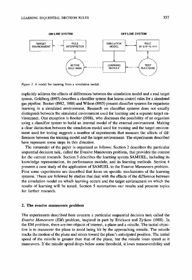
The approach described here reflects a particular methodology for learning via a simulation model. The motivation behind the methodology is that making mistakes on real systems may be costly or dangerous. Since learning may require experimenting with tactical plans that might occasionally produce unacceptable results if applied to the real world, we assume that hypothetical plans will be evaluated in a simulation model (see Figure 1).

Periodically, a plan is extracted from the learning system to represent the learning system's current plan. This plan is tested in the target environment, and the resulting performance is plotted on a learning curve. In principle, this mode of learning might continue indefinitely, with the user periodically updating the decision rules used in the target environment with the current plan suggested by the learning system.

Simulation models have played an important role in several machine learning efforts. The idea of using a simulator to generate examples goes back to Samuel (1963) in the domain of checkers. Buchanan, Sullivan, Cheng and Clearwater (1988), use the RL system to learn error classification rules from a model of a particle beam accelerator, but do not explicitly

L E A R N I N G S E Q U E N T I A L D E C I S I O N R U L E S 357

ON-LINE SYSTEM OFF-LINE SYSTEM

TARGET ~ _ ~ ENVIRONMENT

I I RULE SIMULATION I_ _1 RULE INTERPRETER MODEL ~ INTERPRETER

. . . . . . MODULE

Figure L A mode l for learning f rom a s imulat ion model .

explicitly address the effects of differences between the simulation model and a real target system. Goldberg (1983) describes a classifier system that learns control rules for a simulated gas pipeline. Booker (1982, 1988) and Wilson (1985) present classifier systems for organisms learning in a simulated environment. Research on classifier systems does not usually distinguish between the simulated environment used for learning and a separate target environment. One exception is Booker (1988), who discusses the possibility of an organism using a classifier system to build an internal model of the external environment. Making a clear distinction between the simulation model used for training and the target environment used for testing suggests a number of experiments that measure the effects of differences between the training model and the target environment. The experiments described here represent some steps in this direction.

The remainder of the paper is organized as follows: Section 2 describes the particular sequential decision task, called the Evasive Maneuvers problem, that provides the context for the current research. Section 3 describes the learning system SAMUEL, including its knowledge representation, its performance module, and its learning methods. Section 4 presents a case study of the application of SAMUEL to the Evasive Maneuvers problem. First some experiments are described that focus on specific mechanisms of the learning systems. These are followed by studies that deal with the effects of the difference between the simulation model on which learning occurs and the target environment on which the results of learning will be tested. Section 5 summarizes our results and presents topics for further research.

2. The evasive maneuvers problem

The experiments described here concern a particular sequential decision task called the Evasive Maneuvers (EM) problem, inspired in part by Erickson and Zytkow (1988). In the EM problem, there are two objects of interest, a plane and a missile. The tactial objective is to maneuver the plane to avoid being hit by the approaching missile. The missile tracks the motion of the plane and steers toward the plane's anticipated position. The initial speed of the missile is greater than that of the plane, but the missile loses speed as it maneuvers. If the missile speed drops below some threshold, it loses maneuverability and


drops out of the sky. It is assumed that the plane is more maneuverable than the missile; that is, the plane has a smaller turning radius. There are six sensors that provide information about the current tactical state:

1. last-turn: the current turning rate of the plane. This sensor can assume nine values, ranging from -180 degrees to 180 degrees in 45 degree increments.

2. time: a clock that indicates time since detection of the missile. Assumes integer values between 0 and 19.

3. range: the missile's current distance from the plane. Assumes values from 0 to 1500 in increments of 100.

4. bearing: the direction from the plane to the missile. Assumes integer values from 1 to 12. The bearing is expressed in clock terminology, in which 12 o'clock denotes dead ahead of the plane, and 6 o'clock denotes directly behind the plane.

5. heading: the missile's direction relative to the plane. Assumes values from 0 to 360 in increments of 10 degrees. A heading of 0 (or 360) indicates that the missile is aimed directly at the plane's current position, whereas a heading of 180 means the missile is aimed directly away from the plane.

6. speed: the missile's current speed measured relative to the ground. Assumes values from 0 to 1000 in increments of 50.

Finally, there is a discrete set of actions available to control the plane. In this study, we consider only actions that specify discrete turning rates for the plane. The control variable turn has nine possible settings, between -180 and 180 degrees in 45 degree increments. The learning objective is to develop a tactical plan, i.e., set of decision rules that map current sensor readings into actions, that successfully evades the missile whenever possible.

The EM problem is divided into episodes that begin when the threatening missile is detected and that end when either the plane is hit or the missile is exhausted. It is assumed that the only feedback provided is a numeric payoff, supplied at the end of each episode, that reflects the success of the episode with respect to the goal of evading the missile. The payoff is defined by the formula:

payoff = 1000 if plane escapes missile. = 10t if plane is hit at time t.

The missile may hit the plane any time between 1 and 20 seconds after detection, so the payoff varies from 10 to 200 for unsuccessful episodes to 1000 for successful evasion.

The EM problem is clearly a laboratory-scale model of realistic tactical problems. Never- theless, it includes several features that make it a challenging machine learning problem:

• A weak domain model. It is assumed that the learner has no initial model of the missile. This assumption reflects our interest in learning tactics for environments whose complexity precludes a predictive model of the other agents in the scenario. It is also important to emphasize that having a simulation model of an agent does not imply having a tractable procedure for computing the optimal decision rules for responding to the agent.

LEARNING SEQUENTIAL DECISION RULES 359

• Incomplete state information. The objects in the underlying dynamical system (the plane and the missile) travel through a two-dimensional real space. Since the sensors are discrete, they necessarily provide only a partial representation of the current state. This has important consequences, since the decision-making agent receives all its information through its sensors. Given the many-to-one mapping performed by the sensors, the agent does not have sufficient information in this formulation of the problem to apply techniques such as dynamic programming or the TD method since these methods require unambig- uous state information (Barto, et al., 1989).

• A large state space. While the number of states in the underlying dynamical system is of course infinite, even the number of observable feature vectors defined by the sensors is quite large. Over 25 million distinct feature vectors may be observed, each requiring one of nine possible actions, giving a total of over 225 million maximally specific condition-action pairs. To be useful, the decision rules learned by the system must have a fair amount of generality.

• Delayed payoff. The EM problem assumes that payoff information is available only at the end of an episode. I f feedback were immediately available after each decision, then other well-known methods for learning from examples might apply. However, for complex tactical problems, the level of effort required to develop a reliable critic that gives imme- diate feedback is likely to approximate the manual knowledge engineering effort required to create an optimal set of decision rules. We are interested in developing methods that require less human analytic effort, even at the expense of greater computational effort.

• Noisy sensors. Realistic sensors are likely to suffer from some level of noise that may result in incorrect information about the current state. The presence of noise further com- plicates the learning task.

The following sections present one approach to addressing these challenges.

3. SAMUEL on EM

SAMUEL is a system designed to explore competition-based learning for sequential decision tasks, z SAMUEL consists of three major components: a problem specific module, a performance module, and a learning module. Figure 2 shows the architecture of the system.

The problem specific module consists of the task environment simulation, or world model, and its interfaces. The performance module is called CPS (Competitive Production System), a production system that interacts with the world model by reading sensors, setting control variables, and obtaining payoff from a critic. Like traditional production system interpreters, CPS performs matching and conflict resolution. In addition, CPS performs rule-level assignment of credit based on the intermittent feedback from the critic. The learning module uses a genetic algorithm to develop reactive tactical plans, expressed as a set of condition- action rules. Each plan is evaluated by testing its performance on a number of tasks in the world model. As a result of these evaluations, plans are selected for replication and modification. Genetic operators, such as crossover and mutation, produce plausible new plans from high performance precursors.


PROBLEM SPECIFIC MODULE

,' PERFORMANCE (CPS) MODULE

i i

~ MATCHER ~

~ CONFL,CT ~CORRENT'~ r , ' ~ RESO'OT, ON ~ \ ~N J

~ CREO,T ~ I i ~ ~SS'~"MENT I II

SENSORS

CONTROLS

CRITIC i PLAN . . . . . . . . . . . . . . . . . . . . . . . . . . . . . J_ . . . . . . . . . . . . . . . . . . . . .

FITNESS /

/CU."~TNT~ooM.ET, .G~ GENET.C I~ \ ~ / ~ \ PLANS E --I "LOOR'THM I NEW

~ PLAN

LEARNING MODULE

Figure 2. SAMUEL: A learning system for tactical plans.

The design of SAMUEL owes much to Smith's LS-1 system (Smith, 1980), and draws on some ideas from classifier systems (Holland, 1986; Wilson, 1985; Riolo 1988). In a departure from several previous genetic learning systems, SAMUEL learns rules expressed in a high level rule language. There have been several proposals for applying genetic algorithms to higher level rule languages (Antonisse & Keller, 1987; Bickel & Bickel, 1987; Cramer, 1985; Fujiki & Dickinson, 1987; Koza, 1989), but few empirical results have been reported. The use of a high level language for rules offers several advantages over low level binary pattern languages typically adopted in genetic learning systems. First, it is easier to incorporate existing knowledge, whether acquired from experts or by symbolic learning programs. Second, it is easier to explain the knowledge learned through experience and to transfer the knowledge to human operators. Third, it is possible to combine several forms of learning in a single system: Empirical methods such as genetic algorithms may discover a set of high performance rules, and then an analytic learning method may attempt to explain the success of those rules and thereby enhance an existing partial domain theory (Gordon & Grefenstette, 1990).

The following subsections describe the major modules in more detail, using EM as a concrete example problem. It should be noted that the current version of SAMUEL represents just one way to implement a rule learning system based on genetic algorithms. Although the design of SAMUEL builds on several years of experience with genetic algorithms, we expect that many of the particular learning operators are likely to be modified and generalized as the result of further experience.


3.1. Performance component

The performance module of SAMUEL, CPS, has some similarities to both traditional production system interpreters and to classifier systems. The primary features of CPS are:

• A restricted but high level rule language; • Partial matching; • Competition-driven conflict resolution; and • Incremental credit assignment methods.

These features are described in more detail in the following sections.

3.1.1. Knowledge representation

In contrast with many genetic learning systems, SAMUEL does not apply binary recombination operators to individual rules. Instead, the CROSSOVER operator in SAMUEL recom- bines entire plans by exchanging rules between them. This approach to recombination has both positive and negative implications. The disadvantage is that SAMUEL does not address the important problem of creating new high-level symbols from low-level detector messages, as classifier systems do (Holland, 1986; Booker, 1988). The advantage is that a more natural high-level rule representation may be adopted. Each CPS rule has the form

if (and cl . . . Cn ) then (and a I . . . am)

where each c i is a condition on one of the sensors and each action aj specifies a setting for one of the control variables.

The form of the conditions depends of the type of the sensor. SAMUEL supports four types of sensors: linear, cyclic, structured, and pattern. Linear sensors take on linearly order numeric values. Conditions over linear sensors specify upper and lower bounds for the sensor values. The range of each linear sensor is divided by the user into up to 255 equal segments whose endpoints constitute the legal bounds in the conditions. For example, the speed sensor in EM can take on values over the range 0 to 1000, discretized into 20 equal segments. Thus, an example of a legal condition over speed is

(speed 100 250)

which matches if 100 _< speed <_ 250. In EM, last-turn, time, range, and speed are linear sensors.

Cyclic sensors take on cyclicly ordered numeric values. Like linear sensors, the range of each cycle sensor is divided by the user into equal segments whose endpoints constitute the legal bounds in the conditions. Unlike linear sensors, any pair of legal values can be interpreted as a valid condition for cyclic sensors. In EM, bearing and heading are cyclic


sensors, since the next "higher" value than bearing = 12 is bearing = 1, and the next "higher" value than heading = 350 is heading = 0. The following is a legal condition over heading:

(heading 330 90)

which matches i f 330 _< heading < 360 or i f 0 < heading <_ 90. The rule language of CPS also supports structured nominal sensors whose values are

taken from the nodes of a tree-structured hierarchy. For example, a sensor called weather might be defined to take on values from the following hierarchy:

any

dry wet

sunny cloudy rain snow

Conditions for structured sensors specify a list of values, and the condition matches if the sensor 's current value occurs in a subtree labeled by one of the values in the list. A condition for the weather sensor might be

(weather is [c loudy wet ] )

This would match if weather had value cloudy, wet, rain, or snow. Finally, pattern sensors can take on binary string values. Conditions on pattern sensors

specify patterns over the alphabet {0, 1, #}, as in classifier systems (Holland, 1986). For example, the sensor detector1 might be defined as a eight bi t string, and a condition for this sensor might be

(de tec to r1 00##10#1)

This condition matches i f the string assigned to detector1 agrees with all the positions occu- pied by 0 or 1 in the condition's pattern. The present study uses only numeric (linear and cyclic) sensors, so these other forms will not be discussed further.

The right-hand side of each rule specifies a setting for one or more control variables. For the EM problem, each rule specifies one setting for the variable turn. In general, a given rule may specify conditions for any subset of the sensors and actions for any subset of the control variables. Each rule also has a numeric strength, that serves as a prediction


of the rule's utility (Grefenstette, 1988). The method used to update the rule strengths is described in the section on credit assignment below. A sample rule in the EM system follows:

i f (and ( l a s t - t u r n 0 45) ( t ime 4 14) (range 500 1400) (heading 330 90) (speed 50 850))

then ( t u rn 90) s t r eng th 750

3.1.2. Production system cycle

CPS follows the match/conflict-resolution/act cycle of traditional production systems. A preprocessing phase compiles the rules into match tables so that sensor values index the corresponding match set. However, since there is no guarantee that the current set of rules is in any sense complete, it is important to provide a mechanism for gracefully handling cases in which no rule matches (Booker, 1985). In CPS this is accomplished by assigning each rule a match score equal to the number of conditions it matches. The match set consists of all the rules with the highest current match score. That is, if some rule matches m out of n sensors and no rule matches m + 1 sensors, then the match set consists of all rules with match score m.

Once the match set is computed, an action is selected from the (possibility conflicting) actions recommended by the members of the match set. Each possible action receives a bid equal to the strength of the strongest rule in the match set that specifies that action in its right-hand side. Unlike classifier systems in which all members of the match set vote on which action to perform (Riolo, 1988), CPS selects an action using the probability distribution defined by the strength of the (single) bidder for each action. This prevents a large number of low strength rules from combining to suggest an action that is actually associated with low payoff. All rules in the match set that agree with the selected action are said to be active (Wilson, 1987), and will have their strength adjusted according to the credit assignment algorithm described in the next section.

After conflict resolution, the control variables are set to the values indicated by the selected actions.3 The world model is then advanced by one simulation step. The new state is reflected in a new set of sensor readings, and the entire process repeats.

3.2. Learning methods

Learning in SAMUEL occurs on two distinct levels: credit assignment at the rule level, and genetic competition at the plan level.

3.2.1. Credit assignment

Systems that learn rules for sequential behavior generally face a credit assignment problem: If a sequence of rules fires before the system solves a particular problem, how can


credit or blame be accurately assigned to early rules that set the stage for the final result? Our approach is to assign each rule a measure called strength that serves as a prediction of the expected level of payoff that will be achieved if this rule fires. When payoff is obtained at the end of an episode, the strengths of all active rules (i.e., rules that suggested the actions taken during the current episode) are incrementally adjusted to reflect the current payoff. The adjustment scheme, called the Profit Sharing Plan (PSP), consists of subtract- ing a fraction of the rule's current strength and adding the same fraction of the payoff. The approach is illustrated in Figure 3 with the incremental fraction set to 0.10.

This example shows that rules whose strength correctly predicts the payoff (e.g., R~) retain their original levels of strength, while rules that overestimate the expected payoff (Rz) lose strength and rules that underestimate payoff (R3) gain strength. It has been shown that the PSP computes a time-weighted estimate of the expected external payoff, and that this estimate is useful for conflict resolution (Grefenstette, 1988). However, conflict resolution should take into account not only the expected payoff associated with each rule, but also some measure of our confidence in that estimate. One way to measure confidence is through the variance associated with the estimated payoff. 4 In SAMUEL, the PSP has been adapted to estimate both the mean and the variance of the payoff associated with each rule, as follows: At the end of each episode, the critic provides a payoff r. For each active rule Ri, the estimate of its mean payoff is updated as follows:

/xi = (1 - c)lxi + cr

The estimate of the variance in its payoff is updated similarly:

v i = (1 - c ) l ) i Jr- c ( ~ i - r) 2

The constant c in the equations above is a runtime parameter called the psp rate. If rule R i has an estimated payoff with mean tx i and variance ~], we define the strength of R i as:

s t r e n g t h ( R i ) = ~ i - •i.

Thus, a high strength rule must have both high mean and low variance in its estimated payoff. By biasing conflict resolution toward high-strength rules, we expect to select actions for which we have high confidence of success.

time t

R 1 R 2 R 3 rule

(~)~-1 ' 0 ~ strength

@ = Current State

Figure 3. Updating the strength of rules.


3. 2.2. The genetic algorithm

At the plan level, SAMUEL treats the learning process as a heuristic optimization problem, i.e., a search through a space of knowledge structures looking for structures that lead to high performance. A genetic algorithm is used to perform the search. Genetic algorithms are motivated by standard models of heredity and evolution in the field of population genetics, and embody abstractions of the mechanisms of adaptation present in natural systems (Holland, 1975). Briefly, a genetic algorithm simulates the dynamics of population genetics by maintaining a knowledge base of knowledge structures that evolves over time in response to the observed performance of its knowledge structures in their training environment. Each knowledge structure yields one point in the space of alternative solutions to the problem at hand, which can then be subjected to an evaluation process and assigned a measure of utility (its fitness) reflecting its potential worth as a solution. The search proceeds by repeatedly selecting structures from the current knowledge base on the basis fo fitness, and applying idealized genetic search operators to these structures to produce new structures (offspring) for evaluation. Goldberg (1989) provides a detailed discussion of genetic algorithms. The learning level of SAMUEL is a specialized version of a standard genetic algorithm, GENESIS (Grefenstette, 1986). The remainder of this section outlines the differences between GENESIS and the genetic algorithm in SAMUEL.

3.2.2.1. Adaptive initialization. Two approaches to initializing the knowledge structures of a genetic algorithm have been reported. By far, random initialization of the first population is the most common method. This approach requires the least knowledge acquisition effort, provides a lot of diversity for the genetic algorithm to work with, and presents the maximum challenge to the learning algorithm. Another approach is to seed the initial population with existing knowledge (Grefenstette, 1987). The rule language of SAMUEL was designed to facilitate the inclusion of available knowledge. Future studies with SAMUEL on EM will concern the improvement of manually developed knowledge, but such knowledge was not available for the current study. As a third alternative, we have developed an approach called adaptive initialization. Each plan starts out as a set of completely general rules, but its rules are specialized according to its early experiences. Specifically, each plan in the initial population consists of nine maximally general rules--each such rule says:

for any sensor readings, turn X

where X is one of the nine possible values for the turning rate. A plan consisting of only such rules executes a random walk, since every rule matches on every cycle, and all rules start with equal strength. Although each plan in the initial population executes this random walk policy, it does not follow that they all have the same performance, since the initial conditions for the episodes used to evaluate the plans are selected at random.

In order to introduce plausible new rules, a plan modification operator called SPECIALIZE is applied after each evaluation of a plan. SPECIALIZE is similar in spirit to Holland's trig- gered operators (Holland, 1986). The trigger in this case is the conjunction of the following conditions:


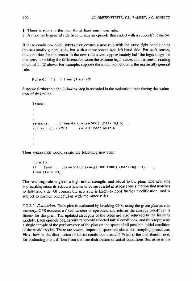
1. There is room in the plan for at least one more rule. 2. A maximally general rule fired during an episode that ended with a successful evasion.

If these conditions hold, SPECIALIZE creates a new rule with the same right-hand side as the maximally general rule, but with a more specialized left-hand side. For each sensor, the condition for the sensor in the new rule covers approximately half the legal range for that sensor, splitting the difference between the extreme legal values and the sensor reading obtained in (2) above. For example, suppose the initial plan contains the maximally general rule:

Ru le 6: i f ( ) t h e n ( t u r n 90)

Suppose further that the following step is recorded in the evaluation trace during the evaluation of this plan:

T r a c e :

s e n s o r s : . . . ( t i m e 4) ( r a n g e 500) ( b e a r i n g 6 ) . . .

a c t i o n : ( t u r n 90) r u l e f i r e d : Ru le 6

Then SPECIALIZE would create the following new rule:

Ru le 10:

i f (and . . . t h e n ( t u r n 90)

( t i m e 2 11) ( r a n g e 300 1000) ( b e a r i n g 3 9) . . . )

The resulting rule is given a high initial strength, and added to the plan. The new rule is plausible, since its action is known to be successful in at least one situation that matches its left-hand side. Of course, the new rule is likely to need further modification, and is subject to further competition with the other rules.

3.2.2.2. Evaluation. Each plan is evaluated by invoking CPS, using the given plan as rule memory. CPS executes a fixed number of episodes, and returns the average payoff as the fitness for the plan. The updated strengths of the rules are also returned to the learning module. Each episode begins with randomly selected initial conditions, and thus represents a single sample of the performance of the plan on the space of all possible initial condition of the world model. There are several important questions about this sampling procedure: First, how is the distribution of initial conditions created? What if the distribution used for evaluating plans differs from the true distribution of initial conditions that arise in the


actual task environment? How many samples must be taken from a given distribution to give the genetic algorithm sufficient information to guide the search for high performance plans? The experiments below address these issues.

3.2.2.3. Selection. Plans are selected for reproduction on the basis of their overall fitness scores returned by CPS. The topic of reproductive selection in genetic algorithms is discussed in the literature (Goldberg, 1989; Grefenstette & Baker, 1989). One new aspect to SAMUEL's selection algorithm concerns the issue of scaling--that is, how to maintain selective pressure as the overall performance rises within the population (Grefenstette, 1986). In SAMUEL, the fitness of each plan is defined as the difference between the average payoff received by the plan and some baseline performance measure. The baseline is adjusted to track the mean payoff received by the population, minus one standard deviation. The baseline is adjusted slowly to provide a moderately consistent measure of fitness. Plans whose payoff fall below the baseline are assigned a fitness measure of 0, resulting in no offspring. This mechanism appears to provide a reasonable way to maintain consistent selective pressure toward higher performance.

3.2.2.4. Genetic operators: CROSSOVER and MUTATION. Selection alone merely produces clones of high performance plans. CROSSOVER works in concert with selection to create plausible new plans. In SAMUEL, CROSSOVER treats rules as indivisible units. Since the rule ordering within a plan is irrelevant, the process of recombination can be viewed as simply selecting rules from each parent to create an offspring plan. Many genetic algorithms permit recombination within individual rules as a way of creating new rules (Smith, 1980; Schaffer, 1984; Holland, 1986). While such operators are easily defined for SAMUEL's rule language (Grefenstette, 1989), we prefer to use CROSSOVER solely to explore the space of rule combinations, and leave rule modification to other operators (i.e., SPECIALIZE and MUTATION).

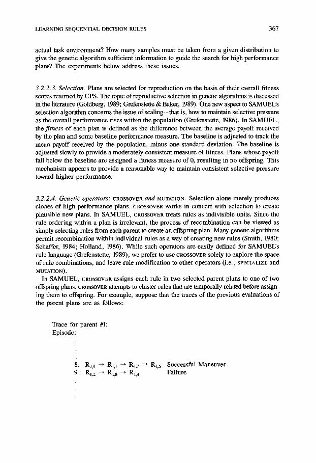
In SAMUEL, CROSSOVER assigns each rule in two selected parent plans to one of two offspring plans. CROSSOVER attempts to cluster rules that are temporally related before assigning them to offspring. For example, suppose that the traces of the previous evaluations of the parent plans are as follows:

Trace for parent #1: Episode:

8. R1, 3 ~ R1,1 -'* R1, 7 ~ R1, 5 Successful Maneuver 9. RI, 2 ~ R1,8 ~ R1, 4 Failure


Trace for parent #2:

4. R2,7 ~ R2,5 Failure 5. R2,6 ~ R2,2 ~ R 2 , 4 Successful Maneuver

where Ri, j is the jth rule in plan i. Then one possible offspring would be:

{ R1,8, . . . , R1,3, R1A, R1,7, RL5 . . . . . R2,6, R2,2, R2,4, - - . , R2,7 }

The idea is that rules that fire in sequence to achieve a successful maneuver should be treated as a group during recombination, in order to increase the likelihood that the offspring plan will inherit some of the better behavior patterns of its parents. Of course, the offspring may not behave identically to either one of its parents, since the probability that a given rule fires depends on the context provided by all the other rules in the plan.

CROSSOVER is restricted so that no plan receives duplicate copies of the same rule. This restriction seems to be necessary to avoid plans containing a large number of copies of the same rule. Given the conflict resolution algorithm in CPS, duplicate copies have no effect on the performance of the plan (other than to take up space), so this restriction seems reasonable. Note that since every rule occurring in either parent is inherited by one of the offspring, any rule that occurs in both parents also occurs in both offspring. The effect is that small groups of rules that are associated with high performance propagate through the population of plans, and serve as building blocks for new plans.

The final genetic operator, MUTATION, introduces new rules by making random changes to existing rules. For example, MUTATION might alter a condition within a rule from ( range 500 1000) to ( range 200 1000), or it might change the action from ( tu rn 45) to (t u r n -90). In the current studies, the new values produced by mutation are chosen randomly from the set of legal values for the given condition or action. Many other forms of mutation are possible. Davis (1989) uses a local mutation operator called cm~Er, that makes only small changes, e.g., from ( range 500 1000) to ( range 400 1000). Future studies with SAMUEL will investigate such operators.

4. Evaluat ion of the m e t h o d

This section presents empirical studies of the performance of SAMUEL on the EM problem. The first two studies focus on aspects of the genetic algorithm itself, and the last two focus on issues concerning the differences between the simulation model and the target environment in which the learned knowledge will be used.


4.L Experimental design

The learning curves shown in this section reflect our assumptions about the methodology of simulation-assisted learning. In particular, we make a distinction between the world model used for learning and the target environment. Let E denote the target environment for which we want to learn decision rules. Let M denote a simulation model of E that can be used for learning. The genetic algorithm in SAMUEL evaluates each plan by measuring the performance of the given plan when solving tasks in model M. At periodic intervals (10 generations in the current experiments), a single plan is extracted from the current population to represent the learning system's current hypothetical plan. The extraction is accomplished by re-evaluating the top 20% of the current population on 100 randomly chosen episodes on the simulation model M. The plan with the best performance in this phase is designated the current hypothesis of the learning system. This plan is tested in the environment E for 100 randomly chosen problem episodes. The plots show the sequence of results of testing on E, using the current plans periodically extracted from the learning system. The assumption is that learning continues indefinitely in the background using system M, while the plan being used on E is periodically updated with the current hypothetical plan of the learning system.

This way of measuring the learning rate of a genetic algorithm is a generalization of the offline performance metric defined by De Jong (1975). In De Jong's work and in later followup studies (Grefenstette, 1986; Schaffer, Caruana, Eshelman & Das, 1989), the offline performance measure assumes that the target environment E is identical to the evaluation model M. Distinguishing these two systems permits the study of how robust the learned plans are if E varies significantly from M, as is likely in practice.

Because SAMUEL employs probabilistic learning methods, all graphs represent the mean performance over 20 independent runs of the genetic algorithm, each run using a different seed for the random number generator. Given our initial assumption that SAMUEL is designed to continue learning indefinitely, it seems inappropriate to compare results by, say, running two variations of the system for a fixed amount of time and comparing the performance of the final plans. Instead, when two learning curves are plotted on the same graph, a vertical line between the curves indicates that there is a statistically significant difference between the means represented by the respective plots (with significance level ot = 0.05). This device allows the reader to see significant differences between two approaches at various points during the learning process.

Unless otherwise noted, all experiments were run with the following parameters in effect: The population contained 100 plans, each plan contained at most 32 rules, the psp rate was 0.01, the crossover rate was 0.8, and the mutation rate was 0.01.

4.2. Tradeoffs between population size and evaluation effort

SAMUEL represents an intensively empirical approach to learning, requiring the evaluation of thousands of alternative plans. Fortunately, genetic algorithms map nicely onto coarse- grained multiprocessors such as the BBN Butterfly. We are currently running SAMUEL on a 128-node Butterfly at the Naval Research Laboratory. By executing a copy of CPS and the world model at each node, up to 128 plans can be evaluated simultaneously.

370 J.j. GREFENSTETTE, C.L. RAMSEY, A.C. SCHULTZ

Two parameters that most directly affect the computational effort required by SAMUEL are the population size and the number of episodes required to evaluate a given plan. Fitz- patrick and Grefenstette (1988) show that genetic algorithms are especially well-suited for problems whose complexity requires the use of statistical techniques in the evaluation phase. This follows from the observation that even if individual plans are evaluated by sampling procedures, the performance estimates associated with the various patterns of rules, or building blocks, in the population are much more accurate than the performance estimates of the individual plans. The implication for SAMUEL is that the amount of problem solving activity required to test individual plans can be fairly limited without adverse effects on the learning rate, as long as the population size is adjusted accordingly. In particular, Fitzpatrick and Grefenstette show that, given a fixed number of samples per generation, it is better to distribute the samples sparsely over a large population than to perform con- centrated sampling over a small population. They validated their analysis with a case study of an image registration problem. In this section, we report the results of similar experiments performed with SAMUEL on the EM problem.

Experiments were performed with SAMUEL on the EM problem to test the effects of varying both the population size and the number of episodes per evaluation. For all runs, the total number of episodes per generation was kept constant. Since the simulation model dominated the computational effort associated with the rest of the system, this means that a single generation took approximately the same amount of time in all runs. Three pairs of parameter settings were tested - - 4, 20 and 100 episodes per evaluation, with corresponding population sizes of 500, 100, and 20, respectively. Results are shown in Figure 4.

Fitzpatrick and Grefenstette report that performance generally improves as the population size increases and the number of samples per evaluation decreases. Our results with SAMUEL are not entirely consistent with their conclusion. However, the differences may be explained by the differences between SAMUEL's genetic algorithm and Fitzpatrick and Grefenstette's. In particular, the clustering phase in SAMUEL's CROSSOVER operator is sen- sitive to the number of episodes per evaluation. When the number of episodes per evaluation is small, clustering is less effective, especially during the early stages of a run when the number of successful episodes is small. Later, when the number of successful episodes increases, more effective clusters can be formed. The effects of clustering can be seen in the shape of the curve for the (population = 500, episodes = 4) case in Figure 4, which starts out slower but eventually catches up to the (population = 100, episodes = 20) case. This is consistent with previous experiments in which clustering contributed to faster learning (Grefenstette, 1988). The runs with (population --- 20, episodes = 100), on the other hand, exhibit rapid improvement early, but taper off when the smaller population converges. This is also consistent with previous genetic algorithms studies that show that small population size cannot support sustained exploration of a large search space. Overall, these results are encouraging in that rapid learning is shown for as few as 20 episodes per evaluation, and this number was adopted for the remaining experiments. The impact of this result is magnified when SAMUEL is run on parallel processors, since it means that the entire population of plans can be evaluated in the time it takes to perform 20 episodes.


0 40 60 8 0 100 120 140 160 180 200

100 100

8 0 - -

Success 60 - - Rate

of Cu r ren t

P lan 40 - -

2 0 - -

0 0

0 200

20

I i I I i I I I I

p = population size e = episodes per evaluat ion

(p,e) = (100, 20)

. . . . . . . . . (p,e) = (20, 100)

. . . . . (p,e) = (500, 4)

l I I i I I I i I 20 40 60 80 100 120 140 160 180

Genera t ions

- 8 0

-60

-40

- 2 0

Figure 4. Tradeoffs between population size and evaluation sampling rate.

4.3. Effects of C R O S S O V E R and M U T A T I O N

An experiment was conducted to test the relative contributions of CROSSOVER and MUTATION in the EM domain. Two sets of runs were conducted, with the only difference being that in one case the CROSSOVER operator was disabled. If CROSSOVER is disabled, then the resulting search looks like a kind of parallel simulated annealing: random changes are made to structures, and the changes are more likely to be kept if they lead to improved performance. The selection pressure in the genetic algorithm serves the same role as temperature in a simulated annealing algorithm: random changes are likely to survive early in the run, but as the average fitness rises, harmful changes are more likely to be rejected (that is, they will not have offspring). This is a much more powerful search method than pure random search, and thus provides a nontrivial baseline against which to measure the full genetic algorithm. The learning curves are shown in Figure 5.

In this case, the difference between the performance of the plans learned with and without CROSSOVER is statistically significant over the entire run. This is consistent with a number of previous studies that show that a genetic algorithm with recombination outperforms a genetic algorithm with mutation alone (Wilson, 1987). Given the many differences between the genetic algorithm in SAMUEL and many previous genetic algorithms, confirmation of this conclusion strengthens our confidence that recombination, even broadly defined, is a powerful search operator.

4.4. Effects of generality of training conditions

Ideally, a simulation model adequately reflects all the important aspects of a target environment. In practice, the validation of a complex simulation model is often very difficult. Consequently, perhaps the most important questions in simulation-assisted learning concern how well knowledge learned using a simulation model transfers to a target environment that


100

8 0 -

S u c c e s s 6 0 - Rate

of Current

Plan 40 -

2 0 -

20 40 60 80 100 120 140 160 180 200

I I I I I I I I I 100

CROSSOVER

. . . . . No CROSSOVER

I I I I I I I [ E 20 40 60 80 100 120 140 160 180

Generations

- - 8 0

- - 6 0

- - 4 0

- - 2 0

200

Figure 5. Effects of CROSSOVER.

differs from the model. One approach to these questions is to study how the plans learned with a given model perform when tested on a variety of target environments. In the next two sections, we perform this kind of sensitivity analysis by using different versions of the simulator in the roles of training model and target environment.

The first experiment concerns the generality of training conditions. Two classes of initial conditions are considered. Let the term f ixed initial conditions mean that each episode begins with the following conditions:

range = 1000 heading = 0 speed = 700 1 <_ bearing <_ 12

These conditions correspond to the missile being placed at a random position along the circumference of a circle of radius 1000, aiming directly at the plane. Let the term variable initial conditions mean that each episode begins with the following conditions:

800 <_ range <~ 1200 - 7 2 _< heading <_ 72 560 < speed <_ 840 1 < bearing <_ 12

That is, each of the first three variables was allowed to randomly vary byup to 20% of the initial values for fixed initial condition, and bearing is again chosen at random. Each class of initial conditions defines an environment. There are four possible experimental conditions, depending on which environment is used for the simulation model and which is used for the target environment, as shown in Table 1.


Table L Experimental conditions over initial conditions.

Target Fixed Target Variable

Model Fixed (Fixed, Fixed) (Fixed, Variable)

Model Variable (Variable, Fixed) (Variable, Variable)

For each experimental condition, the genetic algorithm was executed for 200 generations, using the indicated environments for the simulation model and target environment. The results are shown in Figures 6 and 7.

Figure 6 shows the learning curves for experimental conditions in the first row of Table 1. That is, the training model used by the genetic algorithm presented episodes with fixed initial conditions. The two curves in Figure 6 show the effect of varying the target environment between fixed and variable initial conditions. While the learned plans perform quite well when the training environment matches the target environment, the learned plans perform much less satisfactorily when the target environment includes the more general initial conditions. This is an expected result, given the opportunistic nature of genetic algorithms: The fixed initial conditions in the training model allow, and perhaps even en- courage, the learning system to exploit special features of such scenarios. For example, since the missile speed always has the same initial value, the learning system might reward a plan based on timed responses--Wait three steps and make a hard right turn--that would fail if the initial missile speed were different.

Success Rate

of Current

Plan

100

8 0 -

6 0 -

2

0

20 40 60 80 100 120 140 160 180 200

I I I t _ 1 I I _1_ _r_ _Jloo

, o 40

Tested against variable conds

. . . . . Tested against fixed conds 20

0 I I t I I t I I I 20 40 60 80 100 120 140 160 180 200

Generations

Figure 6 Sensitivity to initial conditions when trained with fixed initial conditions.


100

80- -

Success 60 -- Rate

of Current

Plan 40 -

20--

20 40 60 80 100 1 ~ 140 1 ~ 180 200

I I I I I I I I I t ~

/

Tested against variable conds

. . . . . Tested against fixed conds

-- 80

- - 6 0

- -40

- - 2 0

0 I I I I 1 I I I

20 40 60 80 100 120 140 160 180 200

Generations

Figure 7. Sensitivity to initial conditions when trained with variable initial conditions.

The two curves in Figure 7 show the effect of varying the target environment between fixed and variable initial conditions when the training model has variable initial conditions. In this case, there is a significant difference between the two curves for the first part of the learning session, during which time the learned plans perform better on the target environment with variable initial conditions than on the target environment with fixed initial conditions. A likely interpretation of the latter case is that the learning system initially sees very few instances that match the target environment, and so it is slower to learn appropriate decision rules for that special case.

One may also compare the corresponding curves across Figures 6 and 7. It is clear that, if the target environment has fixed initial conditions, then it is better to have fixed initial conditions in the training model as well. On the other hand, the difference between final portions of the dashed curves in the two figures suggests that it is far less risky to have a training model with overly general initial conditions than to have one with overly restricted initial conditions. If the training model is overly general, then good decision rules can be learned, but at a slower rate.

In order to assess the effects of small changes in the target environments, the best plan from each run in the preceding experiments was tested on 21 target environments in which the initial values for the missile features (range, heading, and speed) for each episode were gradually varied between the fixed initial conditions and the variable initial conditions. Each plan was tested against each environment for 200 episodes, and the results are plotted in Figure 8.

Figure 8 shows that the performance of the plans learned with fixed initial conditions declines steadily as a broader range of initial conditions are encountered, indicating that the learned plans do in fact exploit the regularities of the conditions under which they were trained. Unfortunately, there is no reason to expect SAMUEL to learn plans for situations


0 10 20 30 40 50 60 70 80 90 1 O0

t I [ I I I I I I I loo

80 - " - -- 80

Success 60 - Rate

of Best Plan 40 -

2 0 -

Trained with variable conds

. . . . Trained with fixed conds

- - 60

- - 40

- - 20

0 I I I I I I I I I

10 20 30 40 50 60 70 80 90 100

Percentage of Variation in Initial Conditions in Target Environment

Figure & Performance of learned plans tested against gradually variable initial conditions.

it has not encountered. This is a mixed blessing. It is encouraging that the learning system exploits regularities in its training environment, but this places a burden on the simulation designer to avoid unintended regularities. Figure 8 also shows that the best plans learned with variable initial conditions exhibit high performance over a wide variety of test environments. However, note that the plans learned under variable initial conditions were slightly less effective than the plans learned under fixed initial conditions, when tested against the fixed initial conditions. These results again suggest that training against more general environmental conditions yields slower learning, but the final results are likely to be much more robust.

4.5. Sensi t iv i ty to s e n s o r noise

Noise is an important topic in machine learning research, since real environments cannot be expected to behave as nicely as laboratory ones. While there are many aspects of a real environment that are likely to be noisy, we can identify three major sources of noise in the kind of sequential decision tasks for which SAMUEL is designed: sensor noise, effector noise, and payoff noise. Recall that we assume the performance module cannot directly access the state of the world, but must instead take its input from sensors. Sensor noise refers to errors in sensor data caused by imperfect sensing devices. For example, if the radar indicates that the range to an object is 1000 meters when in fact the range is 875 meters, the performance system has received noisy data. Likewise, we assume that the performance module affects the world by setting the value of control variables, which in turn control effector modules. Effector noise refers to errors arising when effectors fail to perform the action indicated by the current control settings. For example, in the EM world, an effector command might be (turn 45), meaning that the effectors should initiate a 45 degree left


turn. If the plane turns at a different rate, the effector has introduced some noise. An addi- tional source of noise can arise during the learning phase, if the critic gives noisy feedback. For example, a noisy critic might issue a high payoff value for an episode in which the plane is hit. Notice that this third source of noise has a different qualitative character than the first two, since it reflects errors caused by the teacher (or those specifying the desired performance of the system) rather than by the interaction of a performance module with the target environment.

While all of these types of noise are interesting, we restrict our attention to the noise caused by sensors. To test the effects of sensor noise on SAMUEL, two environments were defined. In one environment, the sensors are noise-free. In the second environment, noise is added to each of the four external sensors that indicate the missile's range, bearing, heading, and speed. Noise consists of a random draw from a normal distribution with mean 0.0 and standard deviation equal to 10 % of the legal range for the corresponding sensor. The resulting value is then discretized according to the defined granularity of the sensor. For example, suppose the missile's true heading is 66 degrees. The noise consists of a random draw from a normal distribution with standard deviation 36 (10% of 360 degrees), resulting in a value of, say, 22. The noisy result, 88, is then discretized to the nearest 10 degree boundary (the user-defined granularity of the sensor), and the final sensor reading is 90. As this example shows, the amount of noise in this environment is rather substantial.

As in the previous section, given a noisy environment and a noise-free environment, there are four possible experimental conditions, depending on which environment is used for the simulation model and which is used for the target environment. 5 For each experimental condition, the genetic algorithm was executed for 200 generations, and the results are shown in Figures 9 and 10.

Success Rate

of Cur ren t

P lan

0

100

8 0 - -

6 0 - -

2

0

20 40 60 80 100 120 140 160 180 200

I I I t I I I I I lOO

- ~ - ~ 80

- - 4 0

T e N e d wi th n o i s y s e n s o r s

. . . . . T e s t e d wi th n o i s e - t r e e s e n s o ~ - - 2 0

0 I I I I I I I I I

20 40 60 80 100 120 140 160 180 200

Genera t ions

Figure 9. Sensitivity to sensor noise when trained with noise-free environment.


0 20

I00 I

8 0 -

Success 60 - Rate

of C u r r e n t

Plan 40 -

2 0 -

40 60 80 100 120 140 160 180 200

I I I I I I I I aoo

- - 80

- - 60

- - 40

Tested w i th noisy s e n s o r s

. . . . . Tested w i th noise- f ree sensors - - 20

0 I I I I I I [ I I

20 40 60 80 100 120 140 160 180 200

Genera t ions

Figure 10. Sensitivity to sensor noise when trained with noisy environment.

Once again, these experiments show that SAMUEL learns best when the training environment matches the target environment. Figure 9 shows that plans learned with noise-free sensors do quite poorly when the target environment has noisy sensors. On the other hand, the plans trained under noisy conditions exhibit no significant loss of performance under noise-free conditions, as shown in Figure 10. Note the similarity between Figure 10 and Figure 7. These results suggest that using a training environment that is less regular (in this case, more noisy) than the target environment is better than having a training model with spurious regularities (e.g., noise-free sensors) that do not occur in the target environment.

5. Summary and further research

The studies described here illustrate the kind of investigations one might pursue in simulation- assisted learning with SAMUEL. One important lesson of the empirical studies is that SAMUEL is an opportunistic learner, and will tailor the plans that it learns to the regularities it finds in the training model. It follows that the closer the training model matches the conditions expected in the target environment--in terms of initial conditions and sensor noise--the better the learned plans will be. However, in the absence of a perfect match between training model and target environment, it is better to have too little regularity (e.g., more general initial conditions, more sensor noise) in the training model than to learn with a simulation model with regularities that do not occur in the target environment.

The current results suggest a number of topics that require further work. The following are some of the areas we will focus on in the future.


5.1. Explanation-based learning

The high-performance plans that SAMUEL learns can generate expert behavior that might serve as the input for analytic learning techniques. We would like the system to explain why the plans found by SAMUEL perform well. Our first step is to interpret traces of the behavior of a learned rule set. For example, if the following rule

i f (and ( l a s t - t u r n -135 O) ( t ime 2 16) ( range 0 1000) ( b e a r i n g 6 9) (head ing 50 30) (speed 100 600))

then ( t u r n 45)

fires in a state specified by the feature vector;

( l a s t - t u r n O ) ( t ime 3) ( range 300) ( bea r i ng 3) (heading 290) (speed 400)

then a possible interpretation of this rule firing is:

i f p lane d id not t u r n at t ime ( t - 1) &

m i s s i l e beh ind p lane at t ime t & speed of m i s s i l e =medium at t ime t

then t u rn p lane s o f t l y toward m i s s i l e at t ime t

For the next step, we will construct a domain theory that elaborates and motivates these explanations. We are attempting to adapt Qualitative Process Theory (Forbus, 1984), which provides a language well-suited to describing processes, for the interpretation of the empirical learned rules. The interpretations are expected to be helpful in creating new rules for SAMUEL.

5.2. Generation of plausible initial plans

Currently, the initial plans are generated using a weak model consisting of knowledge about legal values for sensors. We are investigating alternative methods for generation plausible rules using available background knowledge. For example, in the EM domain, we might want to use a Half-Order Theory (Buchanan et al., 1988) to generate symmetric variants of rules. That is, if GENCOVER creates a rule that says, I f the missile is on the left, turn hard left, we may also want to create a rule that says, I f the missile is on the right, turn hard right.

5.3. Traditional rule learning operators

SAMUEL provides a testbed for investigating several rule modification operators besides the genetic operators, such as specialization, generalization, merging, and discrimination (Langley, 1983). We expect that the competitive mechanisms of SAMUEL will enable the


effective use of these operators without making unreasonably strong assumptions about the critic's abili ty to assign credit and blame. We also plan to investigate adaptive methods (Davis, 1989) for selecting which operator to apply.

5.4. More complex problems

The current statement of the EM problem assumes a two-dimensional world. Future experiments will adopt a three-dimensional model and will address problems with multiple control variables, such as controlling both the direction and the speed of the plane. We plan to augment the task environment to test SAMUEL's abili ty to learn control rules for more realistic tactical scenarios. Mult iple incoming threats will be considered, as well as multiple control variables (e.g., accelerations, directions, weapons, etc.).

In summary, experience with S A M U E L indicates that machine learning techniques may enable the design of high performance rules through the interaction of a learning system with a simulation of the task environment. As simulation technology improves, it will become possible to provide learning systems with high fidelity simulations of tasks whose complexity or uncertainty precludes the use of traditional knowledge engineering methods. No matter what the degree of sophistication of the simulator, it is important to assess the effects on any learning method of the differences between the simulation model and the target environment. These initial studies with a simple tactical problem have shown that it is possible for learning systems based on genetic algorithms to effectively search a space of knowledge structures and discover sets of rules that provide high performance in a variety of target environments. Further developments along these lines can be expected to reduce the manual knowledge acquisition effort required to build systems with expert performance on complex sequential decision tasks.

Notes

1. If payoffis accumulated over an infinite period, the total payoffis usually defined to be a (finite) time-weighted sum (Barto, Sutton & Watkins, 1989).

2. SAMUEL stands for Sa'ategy Acquisition Method Using Empirical Learning. The name also honors Art Samuel, one of the pioneers in machine learning.

3. If there is more than one control variable, the conflict resolution phase is executed independently for each control variable. As a result, the settings for different control variables may be recommended by distinct rules. This situation does not arise in EM, since there is only one control variable.

4. The idea of including the variance in the bidding phase in classifier systems was proposed independently by Goldberg (1988).

5. For these experiments, both the noisy and noise-free environment used the variable initial conditions, as described in the previous section.

References

Agre, P.E. & Chapman, D. (1987). Pengi: An implementation of a theory of activity. Proceedings Sixth Na- tional Conference on Artificial Intelligence (pp. 268-272).

Antonisse, H.J. & Keller, K.S. (1987). Genetic operators for high-level knowledge representations. Proceedings of the Second International Conference Genetic Algorithms and Their Applications (pp. 69-76). Cambridge, MA: Erlbaum.


Barto, A.G., Sutton, R.S. & Watkins, C.J.C.H. (1989). Learning and sequential decision making (COINS Technical Report. Amherst, MA: University of Massachusetts.

Bickel, A.S. & Bickel, R.W. (1987). Tree structured rules in genetic algorithms. Proceedings of the Secondlnter- national Conference Genetic Algorithms and Their Applications (pp. 77-81). Cambridge, MA: Erlbaum.

Booker, L.B. (1982). Intelligent behavior as adaptation to the task environment. Doctoral dissertation, Depart- ment of Computer and Communications Sciences, University of Michigan, Ann Arbor, Ann Arbor, MI.

Booker, L.B. (1985). Improving the performance of genetic algorithms in classifier systems. Proceedings of the International Conference Genetic Algorithms and Their Applications (pp. 80-92). Pittsburgh, PA.

Booker, L.B. (1988). Classifier systems that learn internal world models. Machine Learning, 3, 161-192. Buchanan, B.G., Sullivan, J., Cheng, T.P. & Clearwater, S.H. (1988). Simulation-assisted inductive learning.

Proceedings Seventh National Conference on Artificial Intelligence. (pp. 552-557). Cromer, N.L. (1985). A representation for the adaptive generation of simple sequential programs. Proceedings

of the International Conference Genetic Algorithms and Their Applications (pp. 183-187). Pittsburgh, PA. Davis, L. (1989). Adapting operator probabilities in genetic algorithms. Proceedings of the Third International

Conference on Genetic Algorithms. (pp. 61-69). Fairfax, VA: Morgan Kaufmann. De Jong, K.A. (1975). Analysis of the behavior of a class of genetic adaptive systems. Doctoral dissertation, Depart-

ment of Computer and Communications Sciences, University of Michigan, Ann Arbor, Ann Arbor, MI. Erickson, M.D. & Zytkow, J.M. (1988). Utilizing experience for improving the tactical manager. Proceedings

of the Fifth International Conference on Machine Learning. (pp. 444-450). Ann Arbor, MI. Fitzpatrick, M.J. & J.J. Grefenstette (1988). Genetic algorithms in noisy environments, Machine Learning, 3, 101-120. Fujiki, C. & Dickinson, J. (1987). Using the genetic algorithm to generate LISP source code to solve the prisoner's

dilemma. Proceedings of the Second International Conference Genetic Algorithms and Their Applications (pp. 236-240). Cambridge, MA: Erlbaum.

Forbus, K.D. (1984). Qualitative process theory. Artificial Intelligence 24, 85-168. Goldberg, D.E. (1983). Computer-aided gas pipeline operation using genetic algorithms and machine learning.

Doctoral dissertation, Department Civil Engineering, University of Michigan, Ann Arbor, Ann Arbor, MI. Goldberg, D.E. (1988). Probability matching, the magnitude of reinforcement, and classifier system bidding

(Technical Report TCGA-88002). Tuscaloosa, AL: University of Alabama, Department of Engineering Mechanics. Goldberg, D.E. (1989). Genetic algorithms in search, optimization, and machine learning. Reading, MA:

Addison-Wesley. Gordon, D.F. & Grefenstette, J.J. (1990). Explanations of empirically derived reactive plans. Proceedings of the

Seventh International Conference on Machine Learning. Austin, TX: Morgan Kaufmann. Grefenstette, J.J. (1986). Optimization of control parameters for genetic algorithms. IEEE Transactions on Systems,

Man, and Cybernetics, SMC-16(1), 122-128. Grefenstette, J.J. (1987). Incorporating problem specific knowledge into genetic algorithms. In L. Davis (ed.),

Genetic algorithms and simulated annealing. London: Pitman Press. Grefenstette, J.J. (1988). Credit assignment in rule discovery system based on genetic algorithms. Machine Learn-

ing, 3, 225-245. Grefenstette, J.J. (1989). A system for learning control plans with genetic algorithms. Proceedings of the Third

International Conference on Genetic Algorithms. (pp. 183-190). Fairfax, VA: Morgan Kaufmann. Grefenstette, J.J. & Baker, J.E. (1989). How genetic algorithms work: A critical look at implicit parallelism.

Proceedings of the Third International Conference on Genetic Algorithms. (pp. 20-27). Fairfax, VA: Morgan Kaufmann.

Holland, J.H. (1975). Adaptation in natural and artificial systems. Ann Arbor, MI: University Michigan Press. Holland, J.H. (1986). Escaping brittleness: The possibilities of general-purpose learning algorithms applied to

parallel rule-based systems. In R.S. Michalski, J.G. Carbonell, & T. M. Mitchell (Eds.), Machine learning: An artificial intelligence approach (Vol. 2). Los Altos, CA: Morgan Kaufmann.

Koza, J.R. (1989). Hierarchical genetic algorithms operating on populations of computer programs. Proceedings of the Eleventh International Joint Conference on Artificial Intelligence (pp. 768-774). Detroit, MI: Morgan Kaufmann.

Langley, P. (1983). Learning effective search heuristics. Proceedings of the Eighth International Joint Conference on Artificial Intelligence (pp. 419-421). Karlsruhe, Germany: Morgan Kaufmann.

Michalski, R.S. (1983). A theory and methodology for inductive learning. Artificial Intelligence, 20, 111-161.


Mitchell, T.M., Mahadevan, S. & Steinberg, L. (1985). LEAP: A learning apprentice for VLSI design. Proc. Ninth IJCAL (pp. 573-580). Los Angeles: Morgan Kaufmann.

Riolo, R.L. (1988). Empirical studies of default hierarchies and sequences of rules in learning classifier systems, Doctoral dissertation, Department of Electrical Engineering and Computer Science, University of Michigan, Ann Arbor, Ann Arbor, MI.

Samuel, A.L. (1963). Some studies in machine learning using the game of checkers. In E.A. Feigenbaum & J. Feldman, (Eds.), Computer and Thought. McGraw-Hill.

Schaffer, J.D. (1984). Some experiments in machine learning usng vector evaluated genetic algorithms, Doctoral dissertation, Department of Electrical and Biomedical Engineering, Vanderbilt University, Nashville, TN.

Schaffer, J.D., Caruana, R.A. Eshelman, L.J. & Das, R. (1989). A study of control parameters affecting online performance of genetic algorithms for functionl optimization. Proceedings of the Third International Conference on Genetic Algorithms. (pp. 51-60). Fairfax, VA: Morgan Kaufrnann.

Selfridge, O., Sutton, R.S. & Barto, A.G. (1985). Training and tracking in robotics. Proceedings of the Ninth International Conference on Artificial Intelligence. Los Angeles, CA.

Smith, S.E (1980). A learning system based on genetic adaptive algorithms. Doctoral dissertation, Department of Computer Science, University of Pittsburgh, Pittsburgh, PA.

Sutton, R.S. (1988). Learning to predict by the method of temporal differences. Machine Learning, 3, 9-44. W'dson, S.W. (1985). Knowledge growth in an artificial animal. Proceedings of the International Conference Genetic

Algorithms and Their Applications (pp. 16-23). Pittsburgh, PA. Wilson, S.W. (1987). Classifier systems and the animat problem. Machine Learning, 2, 199-228.

learning sequential decision rules using simulation … · learning sequential decision rules using...

Documents