learning real-time perspective patch rectiﬁcation · pdf filelearning real-time perspective...

Noname manuscript No.(will be inserted by the editor)

Learning Real-Time Perspective Patch Rectification

Stefan Hinterstoisser · Vincent Lepetit · Selim Benhimane · Pascal Fua · Nassir

Navab

Received: date / Accepted: date

Abstract We propose two learning-based methods to patch

rectification that are faster and more reliable than state-of-

the-art affine region detection methods. Given a reference

view of a patch, they can quickly recognize it in new views

and accurately estimate the homography between the refer-

ence view and the new view. Our methods are more memory-

consuming than affine region detectors, and are in practice

currently limited to a few tens of patches. However, if the

reference image is a fronto-parallel view and the internal

parameters known, one single patch is often enough to pre-

cisely estimate an object pose. As a result, we can deal in

real-time with objects that are significantly less textured than

the ones required by state-of-the-art methods.

The first method favors fast run-time performance while

the second one is designed for fast real-time learning and ro-

bustness. However, they follow the same general approach:

First, a classifier provides for every keypoint a first estimate

of its transformation. Then, the estimate allows carrying out

an accurate perspective rectification using linear predictors.

The last step is a fast verification—made possible by the ac-

curate perspective rectification—of the patch identity and its

sub-pixel precision position estimation. We demonstrate the

Stefan Hinterstoisser, Selim Benhimane, Nassir Navab

Computer Aided Medical Procedures (CAMP)

Technische Universitat Munchen (TUM)

Boltzmannstrasse 3, 85748 Munich, Germany

Tel.: +49-89-28919400

Fax: +49-89-28917059

E-mail: {hinterst,benhiman,navab}@in.tum.de

Vincent Lepetit, Pascal Fua

Computer Vision Laboratory (CVLab)

Ecole Polytechnique Federale de Lausanne (EPFL)

CH-1015 Lausanne, Switzerland

Tel.: +41-21-6936716

Fax: +41-21-6937520

E-mail: {pascal.fua,vincent.lepetit}@epfl.ch

advantages of our approach on real-time 3D object detection

and tracking applications.

Keywords Patch Rectification · Tracking by Detection ·

Object Recognition · Online Learning · Real-Time

Learning · Pose Estimation

1 Introduction

Retrieving the poses of patches around keypoints in addition

to matching them is an essential task in many applications

such as vision-based robot localization [9], object recogni-

tion [25] or image retrieval [8,24] to constrain the problem

at hand. It is usually done by decoupling the matching pro-

cess from the keypoint pose estimation: The standard ap-

proach is to first use some affine region detector [19] and

then rely on SIFT [16] or SURF [3] descriptors on the recti-

fied regions to match them.

Recently, it has been shown that taking advantage of a

training phase, when possible, greatly improves the speed

and the rate of keypoint recognition tasks [11,22]. Such a

training phase is possible when the application relies on some

database of keypoints, such as object detection or SLAM.

By contrast with Mikolajczyk et al. [19], these learning-

based approaches usually do not rely on the extraction of

local patch transformations in order to handle larger per-

spective distortions but on the ability to generalize well from

training data. The drawback is they only provide a 2–D lo-

cation, while using an affine region detector provides addi-

tional constraints that proved to be useful [25,8].

To overcome this problem we introduce an approach il-

lustrated in Fig. 1 that can provide not only an affine trans-

formation but the full perspective patch rectification and that

is still real-time thanks to a learning stage. We show this is

very useful for object detection and SLAM applications: Ap-

plying our approach on a single keypoint is often enough to

2

(a) (b) (c)

(d) (e) (f)

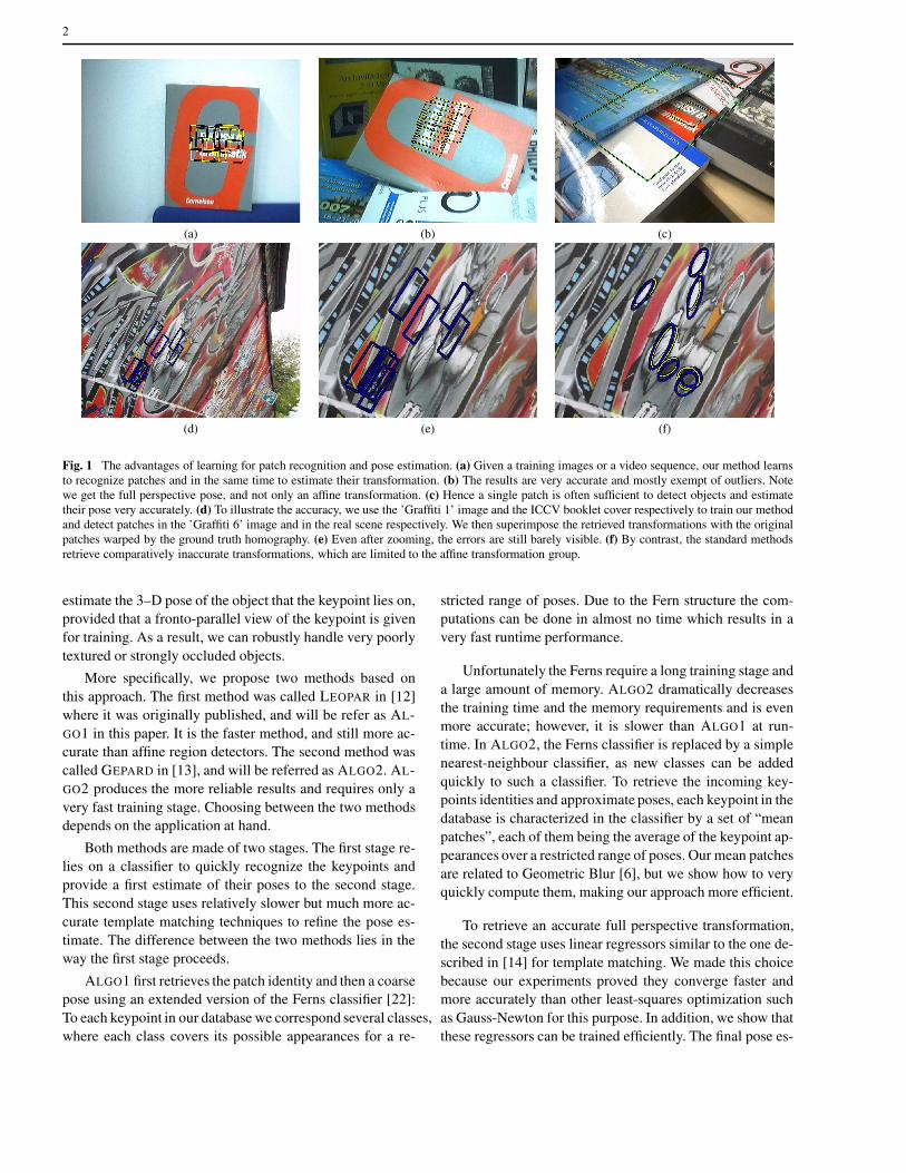
Fig. 1 The advantages of learning for patch recognition and pose estimation. (a) Given a training images or a video sequence, our method learns

to recognize patches and in the same time to estimate their transformation. (b) The results are very accurate and mostly exempt of outliers. Note

we get the full perspective pose, and not only an affine transformation. (c) Hence a single patch is often sufficient to detect objects and estimate

their pose very accurately. (d) To illustrate the accuracy, we use the ’Graffiti 1’ image and the ICCV booklet cover respectively to train our method

and detect patches in the ’Graffiti 6’ image and in the real scene respectively. We then superimpose the retrieved transformations with the original

patches warped by the ground truth homography. (e) Even after zooming, the errors are still barely visible. (f) By contrast, the standard methods

retrieve comparatively inaccurate transformations, which are limited to the affine transformation group.

estimate the 3–D pose of the object that the keypoint lies on,

provided that a fronto-parallel view of the keypoint is given

for training. As a result, we can robustly handle very poorly

textured or strongly occluded objects.

More specifically, we propose two methods based on

this approach. The first method was called LEOPAR in [12]

where it was originally published, and will be refer as AL-

GO1 in this paper. It is the faster method, and still more ac-

curate than affine region detectors. The second method was

called GEPARD in [13], and will be referred as ALGO2. AL-

GO2 produces the more reliable results and requires only a

very fast training stage. Choosing between the two methods

depends on the application at hand.

Both methods are made of two stages. The first stage re-

lies on a classifier to quickly recognize the keypoints and

provide a first estimate of their poses to the second stage.

This second stage uses relatively slower but much more ac-

curate template matching techniques to refine the pose es-

timate. The difference between the two methods lies in the

way the first stage proceeds.

ALGO1 first retrieves the patch identity and then a coarse

pose using an extended version of the Ferns classifier [22]:

To each keypoint in our database we correspond several classes,

where each class covers its possible appearances for a re-

stricted range of poses. Due to the Fern structure the com-

putations can be done in almost no time which results in a

very fast runtime performance.

Unfortunately the Ferns require a long training stage and

a large amount of memory. ALGO2 dramatically decreases

the training time and the memory requirements and is even

more accurate; however, it is slower than ALGO1 at run-

time. In ALGO2, the Ferns classifier is replaced by a simple

nearest-neighbour classifier, as new classes can be added

quickly to such a classifier. To retrieve the incoming key-

points identities and approximate poses, each keypoint in the

database is characterized in the classifier by a set of “mean

patches”, each of them being the average of the keypoint ap-

pearances over a restricted range of poses. Our mean patches

are related to Geometric Blur [6], but we show how to very

quickly compute them, making our approach more efficient.

To retrieve an accurate full perspective transformation,

the second stage uses linear regressors similar to the one de-

scribed in [14] for template matching. We made this choice

because our experiments proved they converge faster and

more accurately than other least-squares optimization such

as Gauss-Newton for this purpose. In addition, we show that

these regressors can be trained efficiently. The final pose es-

3

timate is typically accurate enough to allow a final check by

simple cross-correlation and prune the incorrect results.

Compared to affine region detectors, their closest com-

petitors in the state-of-the-art, our two methods have one

important limitation: They do not scale very well with the

size of the keypoints database, and our current implemen-

tation is limited to a few tens of keypoints to keep the ap-

plications real-time capable. Moreover, they need a frontal

training view and the camera internal parameters to compute

the camera pose with respect to the keypoint. However, as

our experiments show, our two methods are not only much

faster but they also provide an accurate 3–D pose for each

keypoint, by contrast with an approximate affine transforma-

tion. In practice, a single keypoint is often enough to com-

pute the camera or target pose, which compensates this lim-

itation on the database size for the applications we present

in this paper.

In the remainder of the paper, we first discuss related

work. Then, we describe our two methods, and compare

them against affine region detectors [19]. Finally, we present

applications of tracking-by-detection and SLAM using our

method.

2 Related Work

Many different approaches often called “affine region de-

tectors” have been proposed to recognize keypoints under

large perspective distortion. For example, [28] generalized

the Forstner-Harris approach, which was designed to de-

tect keypoints stable under translation, to small similarities

and affine transformations. However, it does not provide the

transformation itself. Other methods attempt to retrieve a

canonical affine transformation without a priori knowledge.

This transformation is then used to rectify the image around

the keypoint and make them easier to recognize. For exam-

ple, [19] showed that the Hessian-Affine detector of [18] and

the MSER detector of [17] are the most reliable ones. In

the case of the Hessian-Affine detector, the retrieved affine

transformation is based on the image second moment ma-

trix. It normalizes the region up to a rotation, which can

then be estimated, for example, by considering the peaks

of the histogram of gradient orientations over the patch as

in SIFT [16]. In the case of the MSER detector, other ap-

proaches exploiting the region shape are also possible [21],

and a common approach is to compute the transformation

from the region covariance matrix and solve for the remain-

ing degree of freedom using local maxima of curvature and

bitangents.

But besides helping the recognition, the estimated affine

transformations can provide useful constraints. For example,

[25] uses them to build and recognize 3–D objects in stereo-

scopic images. [8] uses them to add constraints between the

different regions and help match them more reliably.

Unfortunately, as the experiments presented in this paper

show, the retrieved transformations are often not accurate.

We will show that our learning-based methods can reach a

much better accuracy.

Learning-based methods to recognize keypoints became

quite popular recently, however all the previous methods

provide only the identity of the points, not their pose. For

example, in [15], Randomized Trees are trained with ran-

domly warped patches to estimate a probability distribution

over the classes for each leaf node. The non-terminal nodes

contain decisions based on pairwise intensity comparisons

which are very fast to compute. Once the trees are trained

an incoming patch is classified by adding up the probabil-

ity distributions of the leaf nodes that were reached and by

identifying the class with the maximal probability. However,

training the Randomized Trees is slow and performed of-

fline, which is problematic for applications such as SLAM.

[29] replaced the Randomized Trees by a simpler list struc-

ture and binary values instead of a probability distribution.

These modifications allow them to learn new features online

in real-time. Another approach based on the boosting algo-

rithm presented in [10] to allow online feature learning in

real-time was proposed in [11].

More recently, [27] introduced a learning-based approach

that is closer to the approach presented in this paper. It is

based on what is called “Histogrammed Intensity Patches”

(HIP). The link with our approach is that the HIPs are rem-

iniscent of our “mean patches” used in ALGO2: Each key-

point in the database is represented by a set of HIPs, each

of them computed over a small range of poses. For fast in-

dexing, an HIP is a binarized histogram of the intensities of

a few pixels around the keypoint. However, while this is in

theory possible, estimating the keypoint pose has not been

evaluated nor demonstrated, and this method too provides

only the keypoint identities.

Another work related to this paper is [20], which exploits

the perspective transformation of patches centered on land-

marks in a SLAM application. However, it is still very de-

pendent on the tracking prediction to match the landmarks

and to retrieve their transformations, while we do not need

any prior on the pose. Moreover, in [20], these transforma-

tions are recovered using a Jacobian-based method while, in

our case, a linear predictor can be trained very efficiently for

faster convergence.

In short, to the best of our knowledge, there is no method

in the literature that attempts to reach the exact same goal as

ours. Our two methods can estimate quickly and accurately

the pose of keypoints in a database, thanks to a learning-

based approach.

4

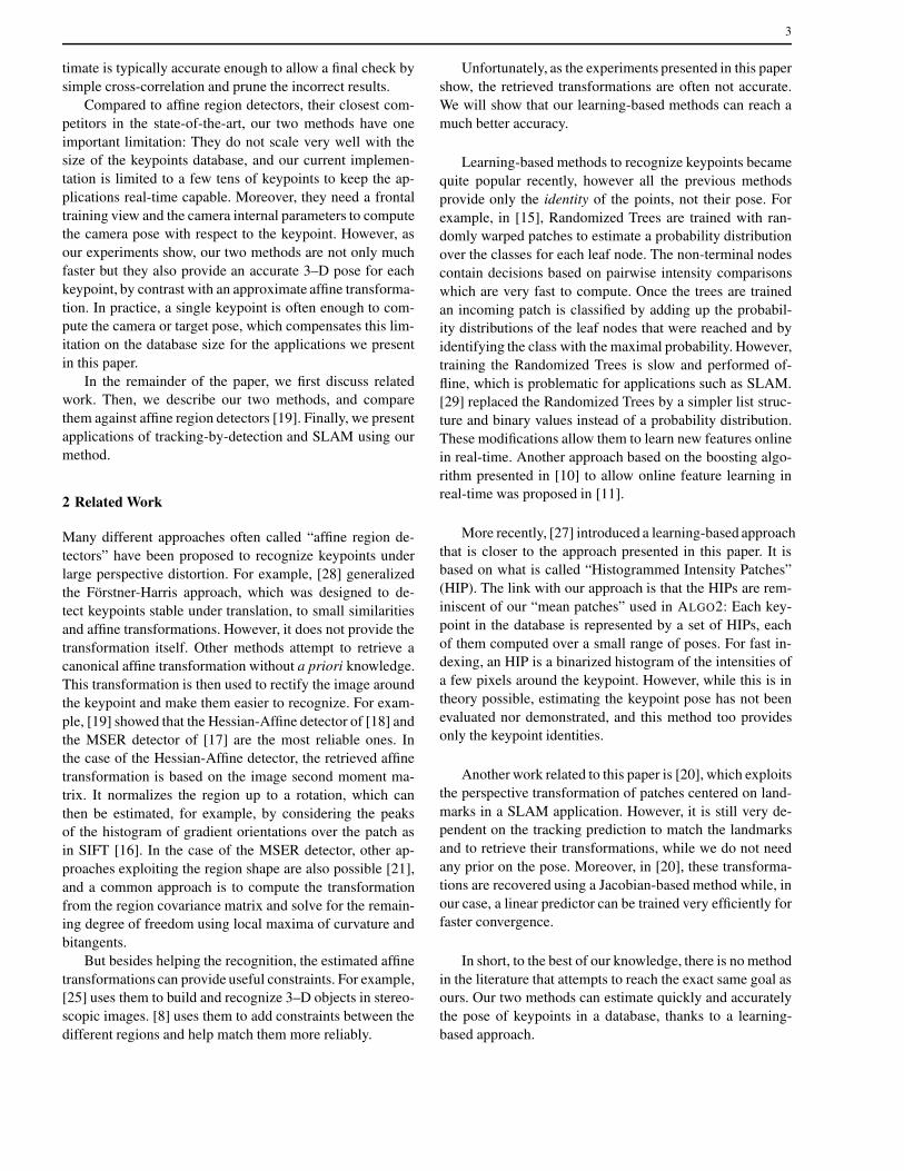
Fig. 2 A first estimate of the patch transformation is obtained using a

classifier that provides the values of the angles ai defined as the angles

between the lines that go through the patch center and each of the four

corners.

(a) (b)

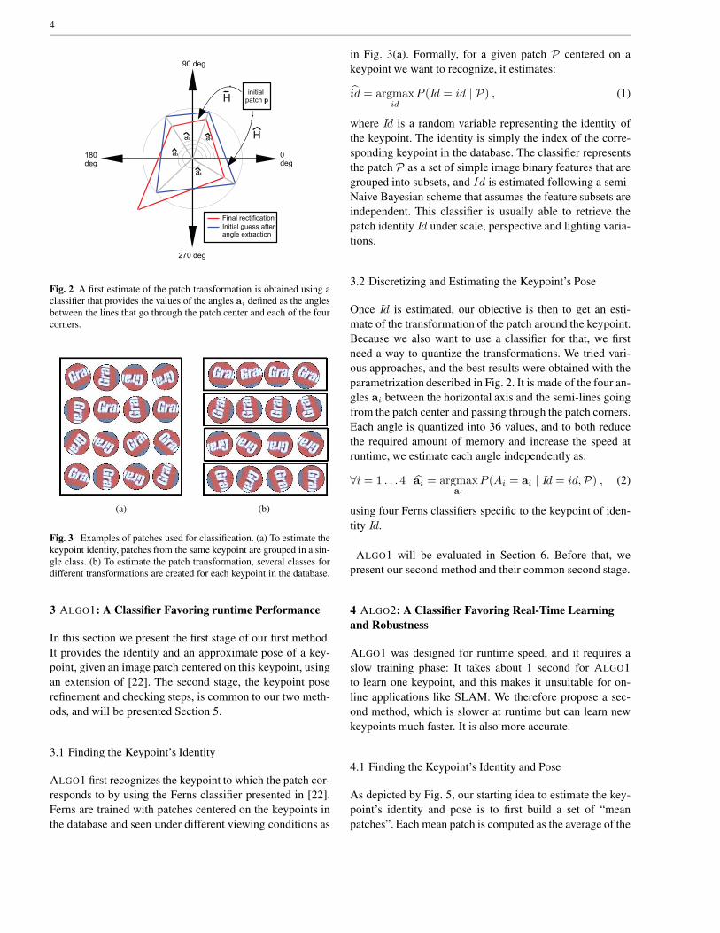
Fig. 3 Examples of patches used for classification. (a) To estimate the

keypoint identity, patches from the same keypoint are grouped in a sin-

gle class. (b) To estimate the patch transformation, several classes for

different transformations are created for each keypoint in the database.

3 ALGO1: A Classifier Favoring runtime Performance

In this section we present the first stage of our first method.

It provides the identity and an approximate pose of a key-

point, given an image patch centered on this keypoint, using

an extension of [22]. The second stage, the keypoint pose

refinement and checking steps, is common to our two meth-

ods, and will be presented Section 5.

3.1 Finding the Keypoint’s Identity

ALGO1 first recognizes the keypoint to which the patch cor-

responds to by using the Ferns classifier presented in [22].

Ferns are trained with patches centered on the keypoints in

the database and seen under different viewing conditions as

in Fig. 3(a). Formally, for a given patch P centered on a

keypoint we want to recognize, it estimates:

id = argmaxid

P (Id = id | P) , (1)

where Id is a random variable representing the identity of

the keypoint. The identity is simply the index of the corre-

sponding keypoint in the database. The classifier represents

the patch P as a set of simple image binary features that are

grouped into subsets, and Id is estimated following a semi-

Naive Bayesian scheme that assumes the feature subsets are

independent. This classifier is usually able to retrieve the

patch identity Id under scale, perspective and lighting varia-

tions.

3.2 Discretizing and Estimating the Keypoint’s Pose

Once Id is estimated, our objective is then to get an esti-

mate of the transformation of the patch around the keypoint.

Because we also want to use a classifier for that, we first

need a way to quantize the transformations. We tried vari-

ous approaches, and the best results were obtained with the

parametrization described in Fig. 2. It is made of the four an-

gles ai between the horizontal axis and the semi-lines going

from the patch center and passing through the patch corners.

Each angle is quantized into 36 values, and to both reduce

the required amount of memory and increase the speed at

runtime, we estimate each angle independently as:

∀i = 1 . . . 4 ai = argmaxai

P (Ai = ai | Id = id,P) , (2)

using four Ferns classifiers specific to the keypoint of iden-

tity Id.

ALGO1 will be evaluated in Section 6. Before that, we

present our second method and their common second stage.

4 ALGO2: A Classifier Favoring Real-Time Learning

and Robustness

ALGO1 was designed for runtime speed, and it requires a

slow training phase: It takes about 1 second for ALGO1

to learn one keypoint, and this makes it unsuitable for on-

line applications like SLAM. We therefore propose a sec-

ond method, which is slower at runtime but can learn new

keypoints much faster. It is also more accurate.

4.1 Finding the Keypoint’s Identity and Pose

As depicted by Fig. 5, our starting idea to estimate the key-

point’s identity and pose is to first build a set of “mean

patches”. Each mean patch is computed as the average of the

5

15 20 25 30 35 40 45 50 55 60 650

10

20

30

40

50

60

70

80

90

100

viewpoint change [deg]

matc

hin

g s

co

re [

%]

ALGO1 classifier trained with homographies

ALGO1−without−correlation


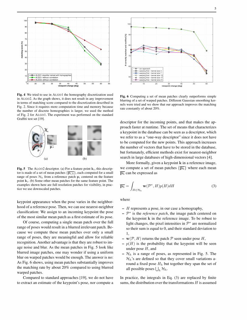
Fig. 4 We tried to use in ALGO1 the homography discretization used

in ALGO2. As the graph shows, it does not result in any improvement

in terms of matching score compared to the discretization described in

Fig. 2. Since it requires more computation time and memory because

the number of discrete homographies is larger, we used the method

of Fig. 2 for ALGO1. The experiment was performed on the standard

Graffiti test set [19].

(a) (b)

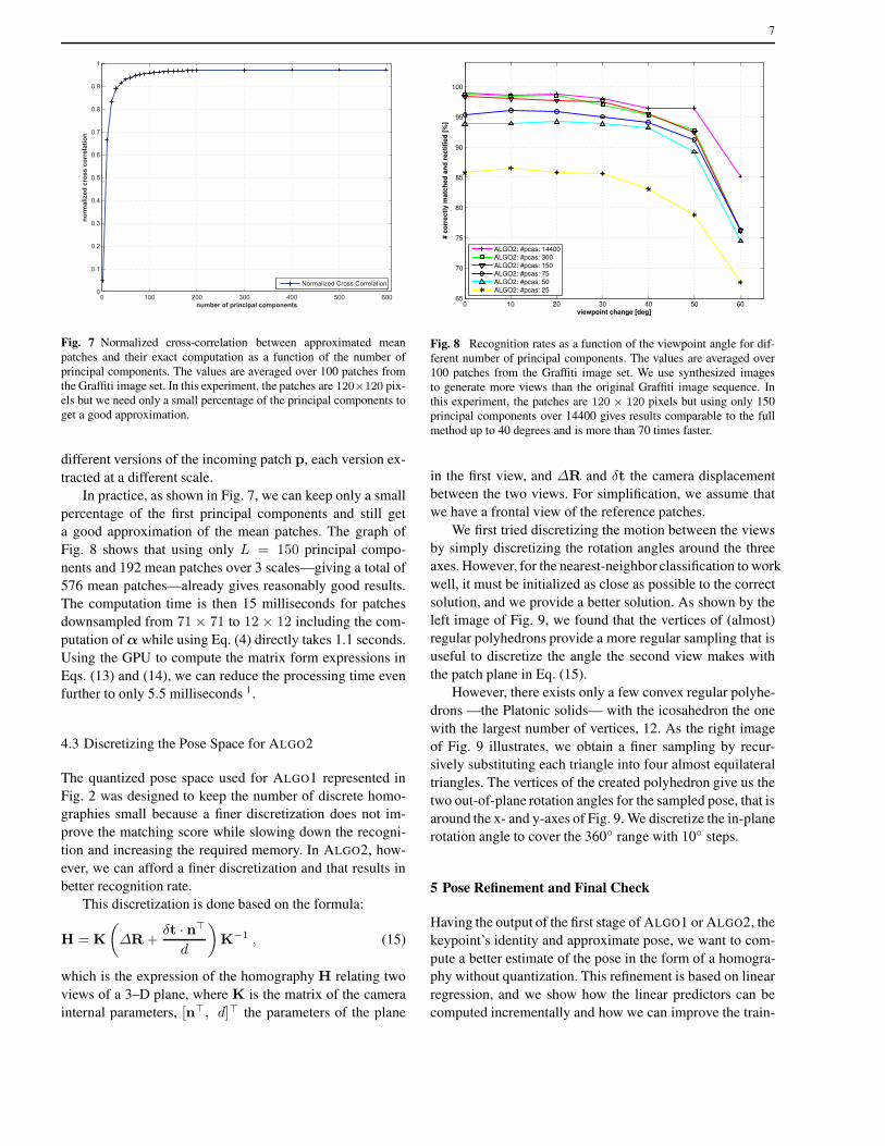
Fig. 5 The ALGO2 descriptor. (a) For a feature point ki, this descrip-

tor is made of a set of mean patches {pi,h}, each computed for a small

range of poses Hh from a reference patch pi centered on the feature

point ki. (b) Some other mean patches for the same feature point. The

examples shown here are full resolution patches for visibility, in prac-

tice we use downscaled patches.

keypoint appearance when the pose varies in the neighbor-

hood of a reference pose. Then, we can use nearest-neighbor

classification: We assign to an incoming keypoint the pose

of the most similar mean patch as a first estimate of its pose.

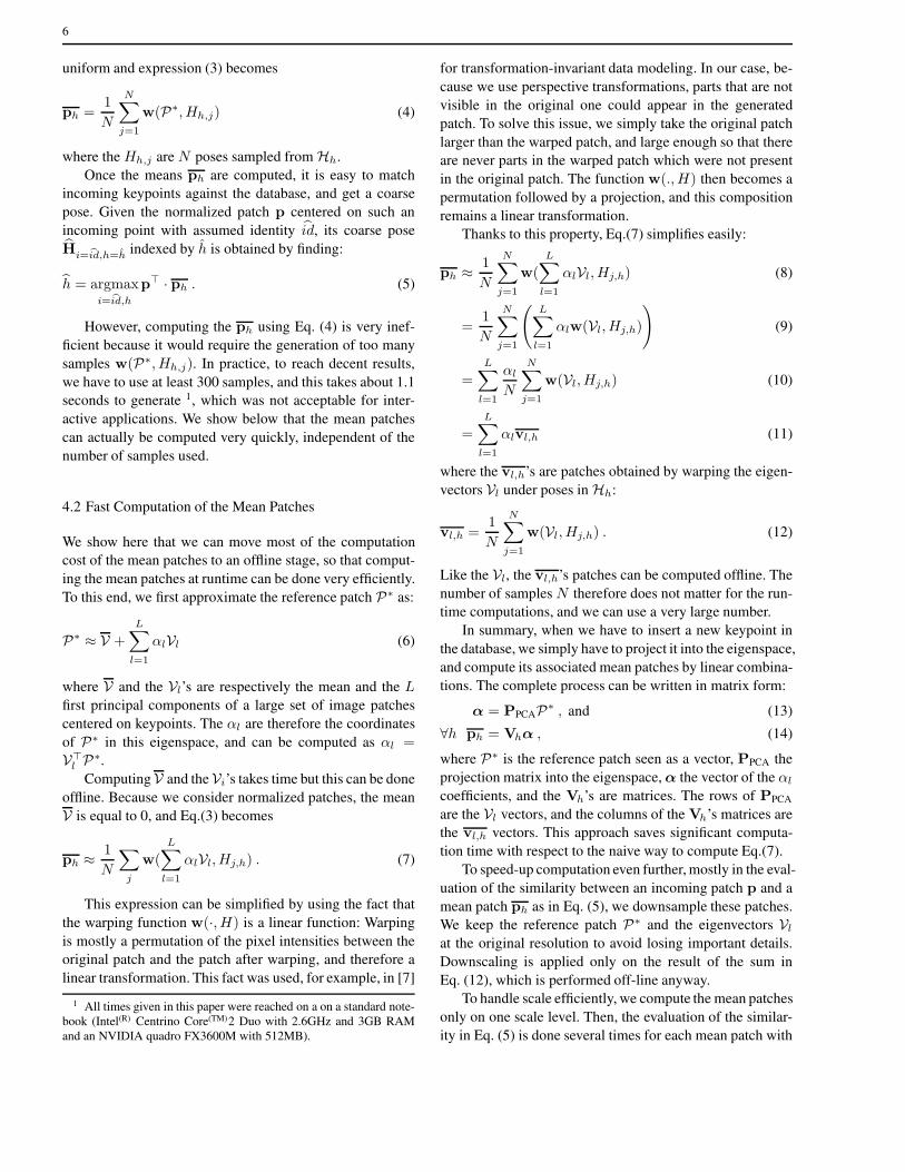
Of course, computing a single mean patch over the full

range of poses would result in a blurred irrelevant patch. Be-

cause we compute these mean patches over only a small

range of poses, they are meaningful and allow for reliable

recognition. Another advantage is that they are robust to im-

age noise and blur. As the mean patches in Fig. 5 look like

blurred image patches, one may wonder if using a uniform

blur on warped patches would be enough. The answer is no:

As Fig. 6 shows, using mean patches substantially improves

the matching rate by about 20% compared to using blurred

warped patches.

Compared to standard approaches [19], we do not have

to extract an estimate of the keypoint’s pose, nor compute a

0 10 20 30 40 50 60

50

60

70

80

90

100


# c

orr

ec

tly

ma

tch

ed

an

d r

ec

tifi

ed

[%

]

our approach

warping first − kernel size 3





Fig. 6 Computing a set of mean patches clearly outperforms simple

blurring of a set of warped patches. Different Gaussian smoothing ker-

nels were tried and we show that our approach improves the matching

rate constantly of about 20%.

descriptor for the incoming points, and that makes the ap-

proach faster at runtime. The set of means that characterizes

a keypoint in the database can be seen as a descriptor, which

we refer to as a “one-way descriptor” since it does not have

to be computed for the new points. This approach increases

the number of vectors that have to be stored in the database,

but fortunately, efficient methods exist for nearest-neighbor

search in large databases of high-dimensional vectors [4].

More formally, given a keypoint k in a reference image,

we compute a set of mean patches {ph} where each mean

ph can be expressed as

ph =

∫

H∈Hh

w(P∗, H)p(H)dH (3)

where

– H represents a pose, in our case a homography,

– P∗ is the reference patch, the image patch centered on

the keypoint k in the reference image. To be robust to

light changes, the pixel intensities in P∗ are normalized

so their sum is equal to 0, and their standard deviation to

1,

– w(P , H) returns the patch P seen under pose H ,

– p(H) is the probability that the keypoint will be seen

under pose H , and

– Hh is a range of poses, as represented in Fig. 5. The

Hh’s are defined so that they cover small variations a-

round a fixed pose Hh but together they span the set of

all possible poses⋃

hHh.

In practice, the integrals in Eq. (3) are replaced by finite

sums, the distribution over the transformations H is assumed

6

uniform and expression (3) becomes

ph =1

N

N∑

j=1

w(P∗, Hh,j) (4)

where the Hh,j are N poses sampled fromHh.

Once the means ph are computed, it is easy to match

incoming keypoints against the database, and get a coarse

pose. Given the normalized patch p centered on such an

incoming point with assumed identity id, its coarse pose

Hi= bid,h=h

indexed by h is obtained by finding:

h = argmaxi= bid,h

p⊤ · ph . (5)

However, computing the ph using Eq. (4) is very inef-

ficient because it would require the generation of too many

samples w(P∗, Hh,j). In practice, to reach decent results,

we have to use at least 300 samples, and this takes about 1.1

seconds to generate 1, which was not acceptable for inter-

active applications. We show below that the mean patches

can actually be computed very quickly, independent of the

number of samples used.

4.2 Fast Computation of the Mean Patches

We show here that we can move most of the computation

cost of the mean patches to an offline stage, so that comput-

ing the mean patches at runtime can be done very efficiently.

To this end, we first approximate the reference patch P∗ as:

P∗ ≈ V +

L∑

l=1

αlVl (6)

where V and the Vl’s are respectively the mean and the L

first principal components of a large set of image patches

centered on keypoints. The αl are therefore the coordinates

of P∗ in this eigenspace, and can be computed as αl =V⊤

l P∗.

ComputingV and theVi’s takes time but this can be done

offline. Because we consider normalized patches, the mean

V is equal to 0, and Eq.(3) becomes

ph ≈1

N

∑

j

w(

L∑

l=1

αlVl, Hj,h) . (7)

This expression can be simplified by using the fact that

the warping function w(·, H) is a linear function: Warping

is mostly a permutation of the pixel intensities between the

original patch and the patch after warping, and therefore a

linear transformation. This fact was used, for example, in [7]

1 All times given in this paper were reached on a on a standard note-

book (Intel(R) Centrino Core(TM)2 Duo with 2.6GHz and 3GB RAM

and an NVIDIA quadro FX3600M with 512MB).

for transformation-invariant data modeling. In our case, be-

cause we use perspective transformations, parts that are not

visible in the original one could appear in the generated

patch. To solve this issue, we simply take the original patch

larger than the warped patch, and large enough so that there

are never parts in the warped patch which were not present

in the original patch. The function w(., H) then becomes a

permutation followed by a projection, and this composition

remains a linear transformation.

Thanks to this property, Eq.(7) simplifies easily:

ph ≈1

N

N∑

j=1

w(

L∑

l=1

αlVl, Hj,h) (8)

=1

N

N∑

j=1

(L∑

l=1

αlw(Vl, Hj,h)

)(9)

=

L∑

l=1

αl

N

N∑

j=1

w(Vl, Hj,h) (10)

=L∑

l=1

αlvl,h (11)

where the vl,h’s are patches obtained by warping the eigen-

vectors Vl under poses inHh:

vl,h =1

N

N∑

j=1

w(Vl, Hj,h) . (12)

Like the Vl, the vl,h’s patches can be computed offline. The

number of samples N therefore does not matter for the run-

time computations, and we can use a very large number.

In summary, when we have to insert a new keypoint in

the database, we simply have to project it into the eigenspace,

and compute its associated mean patches by linear combina-

tions. The complete process can be written in matrix form:

α = PPCAP∗ , and (13)

∀h ph = Vhα , (14)

where P∗ is the reference patch seen as a vector, PPCA the

projection matrix into the eigenspace, α the vector of the αl

coefficients, and the Vh’s are matrices. The rows of PPCA

are the Vl vectors, and the columns of the Vh’s matrices are

the vl,h vectors. This approach saves significant computa-

tion time with respect to the naive way to compute Eq.(7).

To speed-up computation even further, mostly in the eval-

uation of the similarity between an incoming patch p and a

mean patch ph as in Eq. (5), we downsample these patches.

We keep the reference patch P∗ and the eigenvectors Vl

at the original resolution to avoid losing important details.

Downscaling is applied only on the result of the sum in

Eq. (12), which is performed off-line anyway.

To handle scale efficiently, we compute the mean patches

only on one scale level. Then, the evaluation of the similar-

ity in Eq. (5) is done several times for each mean patch with

7

0 100 200 300 400 500 6000

0.1

0.2

0.3

0.4

0.5

0.6

0.7

0.8

0.9

1

number of principal components

no

rma

lize

d c

ros

s c

orr

ela

tio

n

Normalized Cross Correlation

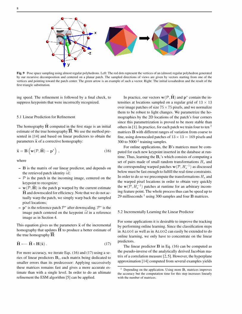
Fig. 7 Normalized cross-correlation between approximated mean

patches and their exact computation as a function of the number of

principal components. The values are averaged over 100 patches from

the Graffiti image set. In this experiment, the patches are 120×120 pix-

els but we need only a small percentage of the principal components to

get a good approximation.

different versions of the incoming patch p, each version ex-

tracted at a different scale.

In practice, as shown in Fig. 7, we can keep only a small

percentage of the first principal components and still get

a good approximation of the mean patches. The graph of

Fig. 8 shows that using only L = 150 principal compo-

nents and 192 mean patches over 3 scales—giving a total of

576 mean patches—already gives reasonably good results.

The computation time is then 15 milliseconds for patches

downsampled from 71 × 71 to 12 × 12 including the com-

putation of α while using Eq. (4) directly takes 1.1 seconds.

Using the GPU to compute the matrix form expressions in

Eqs. (13) and (14), we can reduce the processing time even

further to only 5.5 milliseconds 1.

4.3 Discretizing the Pose Space for ALGO2

The quantized pose space used for ALGO1 represented in

Fig. 2 was designed to keep the number of discrete homo-

graphies small because a finer discretization does not im-

prove the matching score while slowing down the recogni-

tion and increasing the required memory. In ALGO2, how-

ever, we can afford a finer discretization and that results in

better recognition rate.

This discretization is done based on the formula:

H = K

(∆R +

δt · n⊤

d

)K−1 , (15)

which is the expression of the homography H relating two

views of a 3–D plane, where K is the matrix of the camera

internal parameters, [n⊤, d]⊤ the parameters of the plane

0 10 20 30 40 50 6065

70

75

80

85

90

95

100


# c

orr

ectl

y m

atc

hed

an

d r

ecti

fied

[%

]

ALGO2: #pcas: 14400

ALGO2: #pcas: 300

ALGO2: #pcas: 150

ALGO2: #pcas: 75

ALGO2: #pcas: 50

ALGO2: #pcas: 25

Fig. 8 Recognition rates as a function of the viewpoint angle for dif-

ferent number of principal components. The values are averaged over

100 patches from the Graffiti image set. We use synthesized images

to generate more views than the original Graffiti image sequence. In

this experiment, the patches are 120 × 120 pixels but using only 150

principal components over 14400 gives results comparable to the full

method up to 40 degrees and is more than 70 times faster.

in the first view, and ∆R and δt the camera displacement

between the two views. For simplification, we assume that

we have a frontal view of the reference patches.

We first tried discretizing the motion between the views

by simply discretizing the rotation angles around the three

axes. However, for the nearest-neighbor classification to work

well, it must be initialized as close as possible to the correct

solution, and we provide a better solution. As shown by the

left image of Fig. 9, we found that the vertices of (almost)

regular polyhedrons provide a more regular sampling that is

useful to discretize the angle the second view makes with

the patch plane in Eq. (15).

However, there exists only a few convex regular polyhe-

drons —the Platonic solids— with the icosahedron the one

with the largest number of vertices, 12. As the right image

of Fig. 9 illustrates, we obtain a finer sampling by recur-

sively substituting each triangle into four almost equilateral

triangles. The vertices of the created polyhedron give us the

two out-of-plane rotation angles for the sampled pose, that is

around the x- and y-axes of Fig. 9. We discretize the in-plane

rotation angle to cover the 360◦ range with 10◦ steps.

5 Pose Refinement and Final Check

Having the output of the first stage of ALGO1 or ALGO2, the

keypoint’s identity and approximate pose, we want to com-

pute a better estimate of the pose in the form of a homogra-

phy without quantization. This refinement is based on linear

regression, and we show how the linear predictors can be

computed incrementally and how we can improve the train-

8

Fig. 9 Pose space sampling using almost regular polyhedrons. Left: The red dots represent the vertices of an (almost) regular polyhedron generated

by our recursive decomposition and centered on a planar patch. The sampled directions of views are given by vectors starting from one of the

vertices and pointing toward the patch center. The green arrow is an example of such a vector. Right: The initial icosahedron and the result of the

first triangle substitution.

ing speed. The refinement is followed by a final check, to

suppress keypoints that were incorrectly recognized.

5.1 Linear Prediction for Refinement

The homography H computed in the first stage is an initial

estimate of the true homography H. We use the method pre-

sented in [14] and based on linear predictors to obtain the

parameters x of a corrective homography:

x = B(w(P , H)− p∗

), (16)

where

– B is the matrix of our linear predictor, and depends on

the retrieved patch identity id;

– P is the patch in the incoming image, centered on the

keypoint to recognize;

– w(P , H) is the patch p warped by the current estimate

H and downscaled for efficiency. Note that we do not ac-

tually warp the patch, we simply warp back the sampled

pixel locations;

– p∗ is the reference patchP∗ after downscaling.P∗ is the

image patch centered on the keypoint id in a reference

image as in Section 4.

This equation gives us the parameters x of the incremental

homography that updates H to produce a better estimate of

the true homography H:

H←− H ◦H(x) . (17)

For more accuracy, we iterate Eqs. (16) and (17) using a se-

ries of linear predictors Bi, each matrix being dedicated to

smaller errors than its predecessor: Applying successively

these matrices remains fast and gives a more accurate es-

timate than with a single level. In order to do an ultimate

refinement the ESM algorithm [5] can be applied.

In practice, our vectors w(P , H) and p∗ contain the in-

tensities at locations sampled on a regular grid of 13 × 13

over image patches of size 75×75 pixels, and we normalize

them to be robust to light changes. We parametrize the ho-

mographies by the 2D locations of the patch’s four corners

since this parametrization is proved to be more stable than

others in [1]. In practice, for each patch we train four to ten 2

matrices B with different ranges of variation from coarse to

fine, using downscaled patches of 13× 13 = 169 pixels and

300 to 5000 2 training samples.

For online applications, the B’s matrices must be com-

puted for each new keypoint inserted in the database at run-

time. Thus, learning the Bi’s which consists of computing a

set of pairs made of small random transformations Hs and

the corresponding warped patches w(P , H−1s ) as discussed

below must be fast enough to fulfill the real-time constraints.

In order to do so we precompute the transformations Hs and

the warped pixel locations in order to obtain very quickly

the w(P , H−1s ) patches at runtime for an arbitrary incom-

ing feature point. The whole process thus can be speed up to

29 milliseconds 1 using 300 samples and four B matrices.

5.2 Incrementally Learning the Linear Predictor

For some applications it is desirable to improve the tracking

by performing online learning. Since the classification steps

in ALGO1 as well as in ALGO2 can easily be extended to do

online learning, we only have to concentrate on the linear

predictors.

The linear predictor B in Eq. (16) can be computed as

the pseudo-inverse of the analytically derived Jacobian ma-

trix of a correlation measure [2,5]. However, the hyperplane

approximation [14] computed from several examples yields

2 Depending on the application. Using more Bi matrices improves

the accuracy but the computation time for this step increases linearly

with the number of matrices.

9

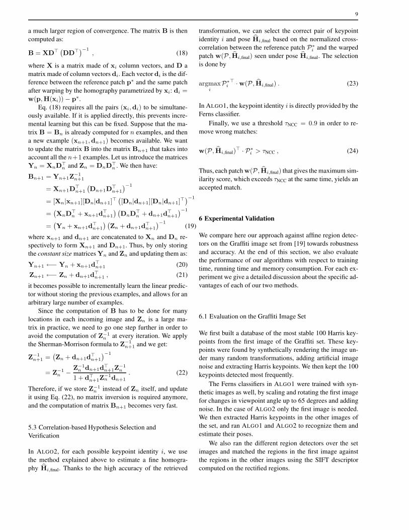
a much larger region of convergence. The matrix B is then

computed as:

B = XD⊤(DD⊤

)−1, (18)

where X is a matrix made of xi column vectors, and D a

matrix made of column vectors di. Each vector di is the dif-

ference between the reference patch p∗ and the same patch

after warping by the homography parametrized by xi: di =

w(p,H(xi))− p∗.

Eq. (18) requires all the pairs (xi,di) to be simultane-

ously available. If it is applied directly, this prevents incre-

mental learning but this can be fixed. Suppose that the ma-

trix B = Bn is already computed for n examples, and then

a new example (xn+1,dn+1) becomes available. We want

to update the matrix B into the matrix Bn+1 that takes into

account all the n+1 examples. Let us introduce the matrices

Yn = XnD⊤n and Zn = DnD⊤

n . We then have:

Bn+1 = Yn+1Z−1

n+1

= Xn+1D⊤n+1

(Dn+1D

⊤n+1

)−1

= [Xn|xn+1][Dn|dn+1]⊤([Dn|dn+1][Dn|dn+1]

⊤)−1

=(XnD⊤

n + xn+1d⊤n+1

) (DnD⊤

n + dn+1d⊤n+1

)−1

=(Yn + xn+1d

⊤n+1

) (Zn + dn+1d

⊤n+1

)−1(19)

where xn+1 and dn+1 are concatenated to Xn and Dn re-

spectively to form Xn+1 and Dn+1. Thus, by only storing

the constant size matrices Yn and Zn and updating them as:

Yn+1 ←− Yn + xn+1d⊤n+1 (20)

Zn+1 ←− Zn + dn+1d⊤n+1 , (21)

it becomes possible to incrementally learn the linear predic-

tor without storing the previous examples, and allows for an

arbitrary large number of examples.

Since the computation of B has to be done for many

locations in each incoming image and Zn is a large ma-

trix in practice, we need to go one step further in order to

avoid the computation of Z−1n at every iteration. We apply

the Sherman-Morrison formula to Z−1

n+1 and we get:

Z−1

n+1 =(Zn + dn+1d

⊤n+1

)−1

= Z−1n −

Z−1n dn+1d

⊤n+1Z

−1n

1 + d⊤n+1Z

−1n dn+1

. (22)

Therefore, if we store Z−1n instead of Zn itself, and update

it using Eq. (22), no matrix inversion is required anymore,

and the computation of matrix Bn+1 becomes very fast.

5.3 Correlation-based Hypothesis Selection and

Verification

In ALGO2, for each possible keypoint identity i, we use

the method explained above to estimate a fine homogra-

phy Hi,final. Thanks to the high accuracy of the retrieved

transformation, we can select the correct pair of keypoint

identity i and pose Hi,final based on the normalized cross-

correlation between the reference patch P∗i and the warped

patch w(P , Hi,final) seen under pose Hi,final. The selection

is done by

argmaxi

P∗i⊤ ·w(P , Hi,final) . (23)

In ALGO1, the keypoint identity i is directly provided by the

Ferns classifier.

Finally, we use a threshold τNCC = 0.9 in order to re-

move wrong matches:

w(P , Hi,final)⊤ · P∗

i > τNCC , (24)

Thus, each patch w(P , Hi,final) that gives the maximum sim-

ilarity score, which exceeds τNCC at the same time, yields an

accepted match.

6 Experimental Validation

We compare here our approach against affine region detec-

tors on the Graffiti image set from [19] towards robustness

and accuracy. At the end of this section, we also evaluate

the performance of our algorithms with respect to training

time, running time and memory consumption. For each ex-

periment we give a detailed discussion about the specific ad-

vantages of each of our two methods.

6.1 Evaluation on the Graffiti Image Set

We first built a database of the most stable 100 Harris key-

points from the first image of the Graffiti set. These key-

points were found by synthetically rendering the image un-

der many random transformations, adding artificial image

noise and extracting Harris keypoints. We then kept the 100

keypoints detected most frequently.

The Ferns classifiers in ALGO1 were trained with syn-

thetic images as well, by scaling and rotating the first image

for changes in viewpoint angle up to 65 degrees and adding

noise. In the case of ALGO2 only the first image is needed.

We then extracted Harris keypoints in the other images of

the set, and ran ALGO1 and ALGO2 to recognize them and

estimate their poses.

We also ran the different region detectors over the set

images and matched the regions in the first image against

the regions in the other images using the SIFT descriptor

computed on the rectified regions.

10

15 20 25 30 35 40 45 50 55 60 650

10

20

30

40

50

60

70

80

90

100


matc

hin

g s

co

re [

%]



Harris Affine

Hessian Affine

MSER

IBR

EBR

15 20 25 30 35 40 45 50 55 60 650

10

20

30

40

50

60

70

80

90

100


matc

hin

g s

co

re [

%]

ALGO1

ALGO2

Harris Affine

Hessian Affine

MSER

IBR

EBR

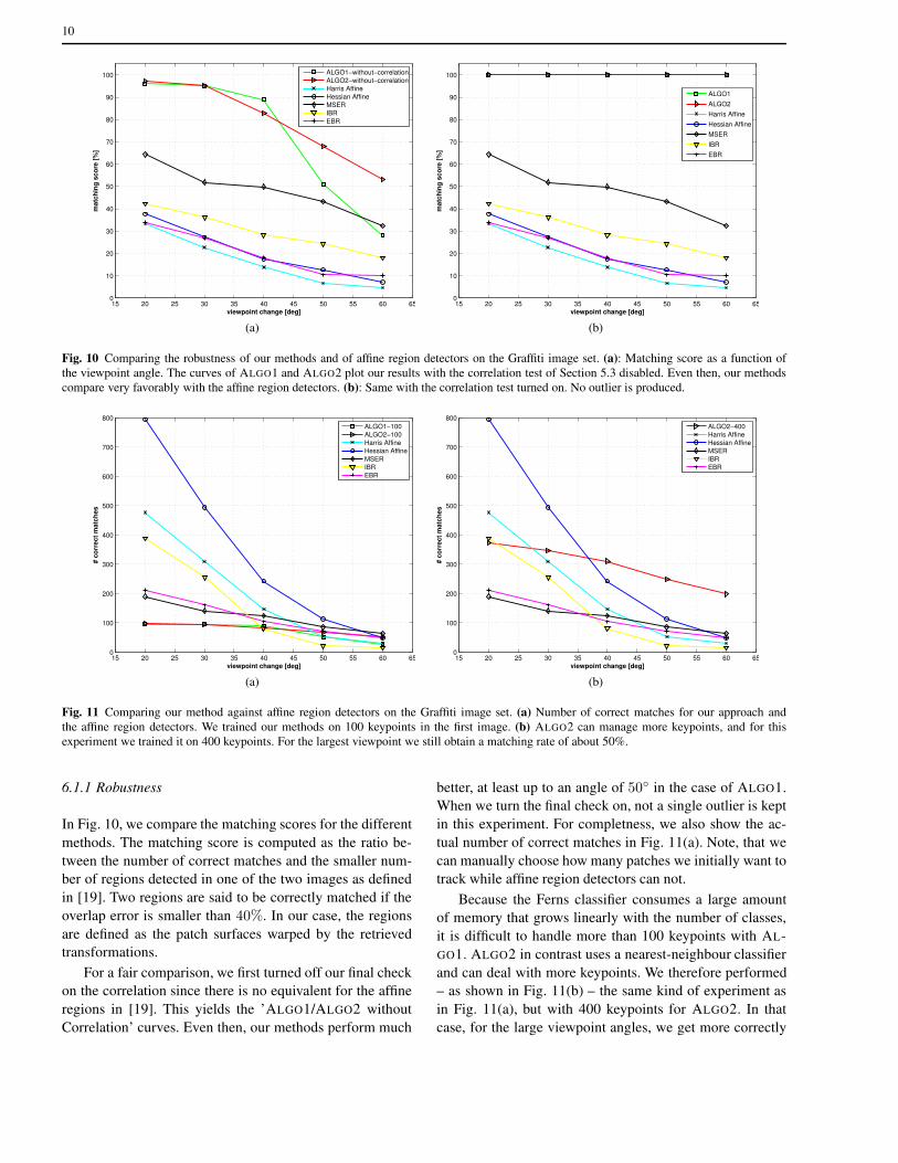
(a) (b)

Fig. 10 Comparing the robustness of our methods and of affine region detectors on the Graffiti image set. (a): Matching score as a function of

the viewpoint angle. The curves of ALGO1 and ALGO2 plot our results with the correlation test of Section 5.3 disabled. Even then, our methods

compare very favorably with the affine region detectors. (b): Same with the correlation test turned on. No outlier is produced.

15 20 25 30 35 40 45 50 55 60 650

100

200

300

400

500

600

700

800


# c

orr

ect

matc

hes

ALGO1−100

ALGO2−100

Harris Affine

Hessian Affine

MSER

IBR

EBR

15 20 25 30 35 40 45 50 55 60 650

100

200

300

400

500

600

700

800


# c

orr

ect

matc

hes

ALGO2−400

Harris Affine

Hessian Affine

MSER

IBR

EBR

(a) (b)

Fig. 11 Comparing our method against affine region detectors on the Graffiti image set. (a) Number of correct matches for our approach and

the affine region detectors. We trained our methods on 100 keypoints in the first image. (b) ALGO2 can manage more keypoints, and for this

experiment we trained it on 400 keypoints. For the largest viewpoint we still obtain a matching rate of about 50%.

6.1.1 Robustness

In Fig. 10, we compare the matching scores for the different

methods. The matching score is computed as the ratio be-

tween the number of correct matches and the smaller num-

ber of regions detected in one of the two images as defined

in [19]. Two regions are said to be correctly matched if the

overlap error is smaller than 40%. In our case, the regions

are defined as the patch surfaces warped by the retrieved

transformations.

For a fair comparison, we first turned off our final check

on the correlation since there is no equivalent for the affine

regions in [19]. This yields the ’ALGO1/ALGO2 without

Correlation’ curves. Even then, our methods perform much

better, at least up to an angle of 50◦ in the case of ALGO1.

When we turn the final check on, not a single outlier is kept

in this experiment. For completness, we also show the ac-

tual number of correct matches in Fig. 11(a). Note, that we

can manually choose how many patches we initially want to

track while affine region detectors can not.

Because the Ferns classifier consumes a large amount

of memory that grows linearly with the number of classes,

it is difficult to handle more than 100 keypoints with AL-

GO1. ALGO2 in contrast uses a nearest-neighbour classifier

and can deal with more keypoints. We therefore performed

– as shown in Fig. 11(b) – the same kind of experiment as

in Fig. 11(a), but with 400 keypoints for ALGO2. In that

case, for the large viewpoint angles, we get more correctly

11

matched keypoints than regions with the affine region detec-

tors.

ALGO2 is also more robust to scale and perspective dis-

tortions than ALGO1. In practice we found out that the limit-

ing factor is by far the repeatability of the keypoint detector.

However, once a keypoint is correctly detected, it is very

frequently correctly matched at least by ALGO2.

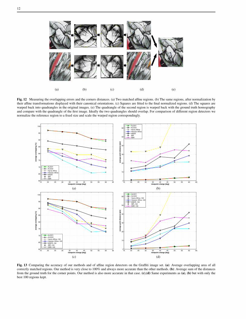
6.1.2 2–D Accuracy

In Figs. 13(a)-(d), we compare the 2–D accuracy for the dif-

ferent methods. To create these graphs, we proceed as shown

in Fig. 12. We first fit a square tangent to the normalized re-

gion, take into account the canonical orientation retrieved by

SIFT and warp these squares back with the inverse transfor-

mation to get a quadrangle. To account for different scales,

we proceed as in [19]: We normalize the reference patch and

the back-warped quadrangle such that the size of the refer-

ence patch is the same for all the patches.

Two corresponding regions should overlap if one of them

is warped using the ground truth homography. A perfect

overlap for the affine regions cannot be expected since their

detectors are unable to retrieve the full perspective. Since in

SIFT several orientations were considered when ambiguity

arises, we decided to keep the one that yields the most accu-

rate correspondence. In the case of our method, the quadran-

gles are simply taken to be the patch borders after warping

by the retrieved transformations.

Fig. 13(a) evaluates the error based on the overlap be-

tween the quadrangles and their corresponding warped ver-

sions. This overlap is between 90% and 100% for our meth-

ods, about 5-10% better than MSER and about 15-25% bet-

ter for the other methods. Fig. 13(b) evaluates the error based

on the distances between the quadrangle corners. Our meth-

ods also perform much better than the other methods. The

error of the patch corner is less than two pixels in average for

ALGO1 and slightly more for ALGO2. Figs. 10(c) and (d)

show the same comparisons, this time when taking only the

best 100 regions into account. The results are very similar.

6.2 3–D Pose Evaluation for Low-Textured Objects

In order to demonstrate the usefulness of our approach espe-

cially for low textured objects and for outdoor environments,

we did two other quantitative experiments.

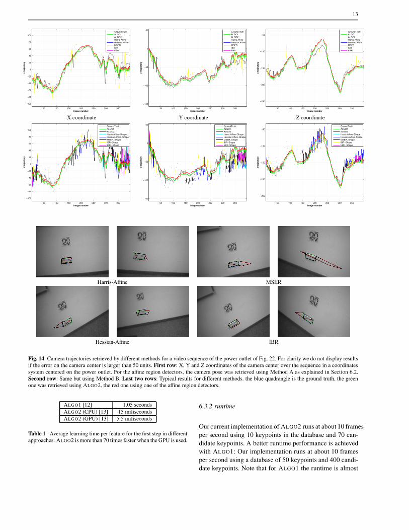
For the first experiment we ran different methods to re-

trieve the camera pose using the power outlet of Fig. 14

in a sequence of 398 real images. To obtain ground truth

data we attached an artificial marker next to the power out-

let and tracked this marker. The marker itself was hidden in

the reference image. We consider errors on the camera cen-

ter larger than 50 units as not correctly matched. For clarity

we do not display these false results. For our approaches we

learned only one single patch on the power outlet to track

in order to emphasize the possibility to track an object with

only a single patch. ALGO2 achieved a successful matching

rate in over 98%, directly followed by ALGO1 with 97%.

For the affine region detectors we tried two different

methods to estimate the pose of the power outlet:

– Method A: For the first row of Fig. 14 we computed the

pose from the 2–D locations of all the correctly matched

affine regions. The correct matches were obtained by

computing the overlap error between the regions that

were matched by SIFT. In order to compute the over-

lap error we used the ground truth transformations. Note

that this gives a strong advantage to the affine region de-

tectors since the ground truth is usually not available.

Each pair of regions was labeled as correctly matched

if the overlap error was below 40%. The IBR detector

obtained the best results with a 18% matching rate.

– Method B: For the second row, we used the shape of two

matched affine regions in order to determine the current

pose of the object. In order to obtain the missing de-

gree of freedom, the orientation was obtained by deter-

mining the dominant orientation within the patch [16].

Since for each image several transformations are avail-

able due to several extracted affine regions, we took the

transformation that corresponds best to the ground truth.

The MSER and the Hessian-Affine detector perform best

with a matching rate of 43% and 35%.

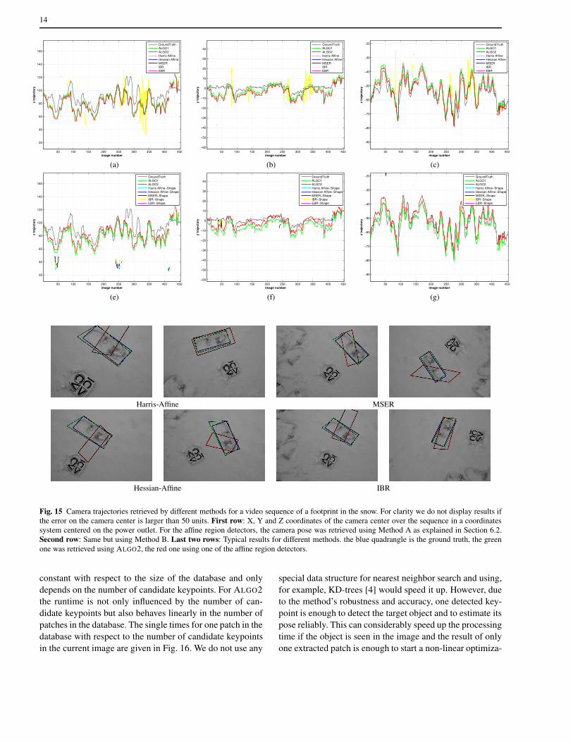
For the second experiment, shown in Fig. 15, we tracked

a foot print in a snowy ground in a sequence of 453 images.

The results are very similar to the first experiment’s results.

The success rates of our algorithms are around 88%. Again,

Method A with the IBR detector performs best among the

affine region detectors with a matching rate of 12%. All

other detectors had success rates of below 1%. For Method

B, all affine region detectors performed around 5% except

the EBR detector which had a matching rate below 1%.

6.3 Speed

We give below the computation times for training and run-

time for both of our methods. All times given were obtained

on a standard notebook 1. Our implementations are written

in C++ using the Intel OpenCV and IPP libraries.

6.3.1 Training

Table 1 shows the advantage of ALGO2 over ALGO1: It is

much faster than ALGO1. When the GPU is used, learning

time drops to 5.5 milliseconds, which is largely fast enough

for frame rate learning, for SLAM applications for example.

Computing the B’s matrices for the refinement stage can be

done in an additional 29 ms on the CPU.

12

(a) (b) (c) (d) (e)

Fig. 12 Measuring the overlapping errors and the corners distances. (a) Two matched affine regions. (b) The same regions, after normalization by

their affine transformations displayed with their canonical orientations. (c) Squares are fitted to the final normalized regions. (d) The squares are

warped back into quadrangles in the original images. (e) The quadrangle of the second region is warped back with the ground truth homography

and compare with the quadrangle of the first image. Ideally the two quadrangles should overlap. For comparison of different region detectors we

normalize the reference region to a fixed size and scale the warped region correspondingly.

15 20 25 30 35 40 45 50 55 60 6560

65

70

75

80

85

90

95

100


avera

ge o

verl

ap

pin

g [

%]

ALGO1

ALGO2

Harris Affine

Hessian Affine

MSER

IBR

EBR

15 20 25 30 35 40 45 50 55 60 650

10

20

30

40

50

60


avera

ge p

oin

t d

ista

nce [

pix

]

ALGO1

ALGO2

Harris Affine

Hessian Affine

MSER

IBR

EBR

(a) (b)

15 20 25 30 35 40 45 50 55 60 6560

65

70

75

80

85

90

95

100


avera

ge o

verl

ap

pin

g [

%]

ALGO1

ALGO2

Harris Affine−100

Hessian Affine−100

MSER−100

IBR−100

EBR−100

15 20 25 30 35 40 45 50 55 60 650

10

20

30

40

50

60


avera

ge p

oin

t d

ista

nce [

pix

]

ALGO1

ALGO2

Harris Affine−100

Hessian Affine−100

MSER−100

IBR−100

EBR−100

(c) (d)

Fig. 13 Comparing the accuracy of our methods and of affine region detectors on the Graffiti image set. (a): Average overlapping area of all

correctly matched regions. Our method is very close to 100% and always more accurate than the other methods. (b): Average sum of the distances

from the ground truth for the corner points. Our method is also more accurate in that case. (c),(d) Same experiments as (a), (b) but with only the

best 100 regions kept.

13

50 100 150 200 250 300 350

−100

−80

−60

−40

−20

0

20

40

60

80

100

image number

x t

raje

cto

ry

GroundTruth

ALGO1

ALGO2

Harris Affine

Hessian Affine

MSER

IBR

EBR

50 100 150 200 250 300 350

−150

−100

−50

0

50

image number

y t

raje

cto

ry

GroundTruth

ALGO1

ALGO2

Harris Affine

Hessian Affine

MSER

IBR

EBR

50 100 150 200 250 300 350

−250

−200

−150

−100

−50

image number

z t

raje

cto

ry

GroundTruth

ALGO1

ALGO2

Harris Affine

Hessian Affine

MSER

IBR

EBR

X coordinate Y coordinate Z coordinate

50 100 150 200 250 300 350

−100

−80

−60

−40

−20

0

20

40

60

80

100

image number

x t

raje

cto

ry

GroundTruth

ALGO1

ALGO2

Harris Affine−Shape

Hessian Affine−Shape

MSER−Shape

IBR−Shape

EBR−Shape

50 100 150 200 250 300 350

−150

−100

−50

0

50

image number

y t

raje

cto

ry

GroundTruth

ALGO1

ALGO2



MSER−Shape

IBR−Shape

EBR−Shape

50 100 150 200 250 300 350

−250

−200

−150

−100

−50

image number

z t

raje

cto

ry

GroundTruth

ALGO1

ALGO2



MSER−Shape

IBR−Shape

EBR−Shape

Harris-Affine MSER

Hessian-Affine IBR

Fig. 14 Camera trajectories retrieved by different methods for a video sequence of the power outlet of Fig. 22. For clarity we do not display results

if the error on the camera center is larger than 50 units. First row: X, Y and Z coordinates of the camera center over the sequence in a coordinates

system centered on the power outlet. For the affine region detectors, the camera pose was retrieved using Method A as explained in Section 6.2.

Second row: Same but using Method B. Last two rows: Typical results for different methods. the blue quadrangle is the ground truth, the green

one was retrieved using ALGO2, the red one using one of the affine region detectors.

ALGO1 [12] 1.05 seconds

ALGO2 (CPU) [13] 15 miliseconds

ALGO2 (GPU) [13] 5.5 miliseconds

Table 1 Average learning time per feature for the first step in different

approaches. ALGO2 is more than 70 times faster when the GPU is used.

6.3.2 runtime

Our current implementation of ALGO2 runs at about 10 frames

per second using 10 keypoints in the database and 70 can-

didate keypoints. A better runtime performance is achieved

with ALGO1: Our implementation runs at about 10 frames

per second using a database of 50 keypoints and 400 candi-

date keypoints. Note that for ALGO1 the runtime is almost

14

50 100 150 200 250 300 350 400 450

20

40

60

80

100

120

140

160

image number

x t

raje

cto

ry

GroundTruth

ALGO1

ALGO2

Harris Affine

Hessian Affine

MSER

IBR

EBR

50 100 150 200 250 300 350 400 450

−60

−50

−40

−30

−20

−10

0

10

20

30

40

image number

y t

raje

cto

ry

GroundTruth

ALGO1

ALGO2

Harris Affine

Hessian Affine

MSER

IBR

EBR

50 100 150 200 250 300 350 400 450

−90

−80

−70

−60

−50

−40

−30

−20

image number

z t

raje

cto

ry

GroundTruth

ALGO1

ALGO2

Harris Affine

Hessian Affine

MSER

IBR

EBR

(a) (b) (c)

50 100 150 200 250 300 350 400 450

20

40

60

80

100

120

140

160

image number

x t

raje

cto

ry

GroundTruth

ALGO1

ALGO2



MSER−Shape

IBR−Shape

EBR−Shape

50 100 150 200 250 300 350 400 450

−60

−50

−40

−30

−20

−10

0

10

20

30

40

image number

y t

raje

cto

ry

GroundTruth

ALGO1

ALGO2



MSER−Shape

IBR−Shape

EBR−Shape

50 100 150 200 250 300 350 400 450

−90

−80

−70

−60

−50

−40

−30

−20

image number

z t

raje

cto

ry

GroundTruth

ALGO1

ALGO2



MSER−Shape

IBR−Shape

EBR−Shape

(e) (f) (g)

Harris-Affine MSER

Hessian-Affine IBR

Fig. 15 Camera trajectories retrieved by different methods for a video sequence of a footprint in the snow. For clarity we do not display results if

the error on the camera center is larger than 50 units. First row: X, Y and Z coordinates of the camera center over the sequence in a coordinates

system centered on the power outlet. For the affine region detectors, the camera pose was retrieved using Method A as explained in Section 6.2.

Second row: Same but using Method B. Last two rows: Typical results for different methods. the blue quadrangle is the ground truth, the green

one was retrieved using ALGO2, the red one using one of the affine region detectors.

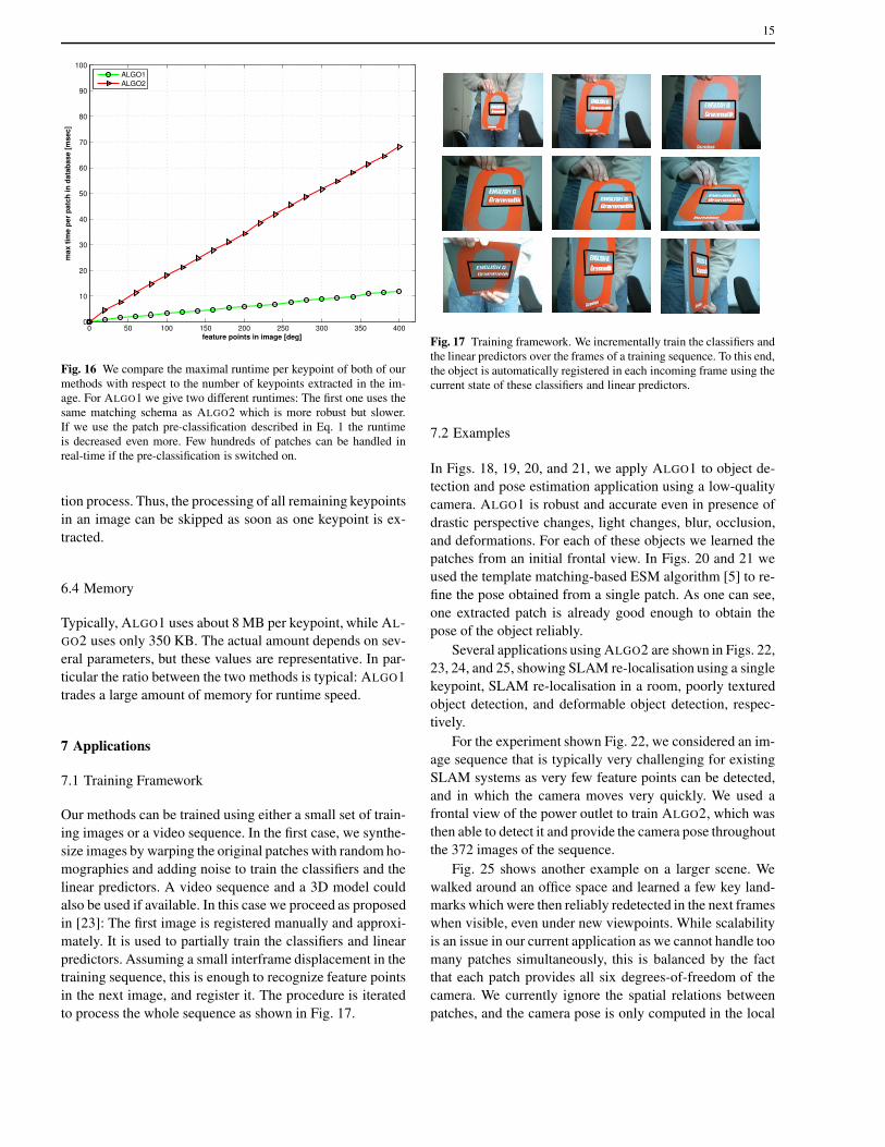
constant with respect to the size of the database and only

depends on the number of candidate keypoints. For ALGO2

the runtime is not only influenced by the number of can-

didate keypoints but also behaves linearly in the number of

patches in the database. The single times for one patch in the

database with respect to the number of candidate keypoints

in the current image are given in Fig. 16. We do not use any

special data structure for nearest neighbor search and using,

for example, KD-trees [4] would speed it up. However, due

to the method’s robustness and accuracy, one detected key-

point is enough to detect the target object and to estimate its

pose reliably. This can considerably speed up the processing

time if the object is seen in the image and the result of only

one extracted patch is enough to start a non-linear optimiza-

15

0 50 100 150 200 250 300 350 4000

10

20

30

40

50

60

70

80

90

100

feature points in image [deg]

max t

ime p

er

patc

h in

data

base [

msec]

ALGO1

ALGO2

Fig. 16 We compare the maximal runtime per keypoint of both of our

methods with respect to the number of keypoints extracted in the im-

age. For ALGO1 we give two different runtimes: The first one uses the

same matching schema as ALGO2 which is more robust but slower.

If we use the patch pre-classification described in Eq. 1 the runtime

is decreased even more. Few hundreds of patches can be handled in

real-time if the pre-classification is switched on.

tion process. Thus, the processing of all remaining keypoints

in an image can be skipped as soon as one keypoint is ex-

tracted.

6.4 Memory

Typically, ALGO1 uses about 8 MB per keypoint, while AL-

GO2 uses only 350 KB. The actual amount depends on sev-

eral parameters, but these values are representative. In par-

ticular the ratio between the two methods is typical: ALGO1

trades a large amount of memory for runtime speed.

7 Applications

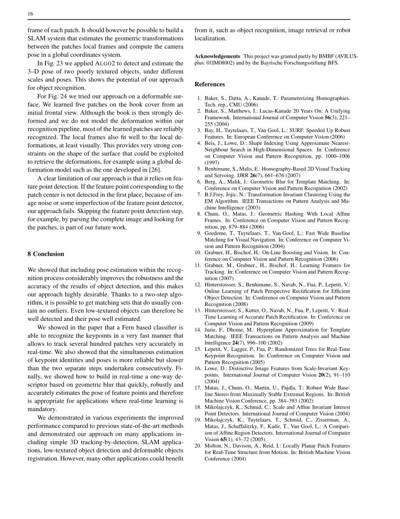
7.1 Training Framework

Our methods can be trained using either a small set of train-

ing images or a video sequence. In the first case, we synthe-

size images by warping the original patches with random ho-

mographies and adding noise to train the classifiers and the

linear predictors. A video sequence and a 3D model could

also be used if available. In this case we proceed as proposed

in [23]: The first image is registered manually and approxi-

mately. It is used to partially train the classifiers and linear

predictors. Assuming a small interframe displacement in the

training sequence, this is enough to recognize feature points

in the next image, and register it. The procedure is iterated

to process the whole sequence as shown in Fig. 17.

Fig. 17 Training framework. We incrementally train the classifiers and

the linear predictors over the frames of a training sequence. To this end,

the object is automatically registered in each incoming frame using the

current state of these classifiers and linear predictors.

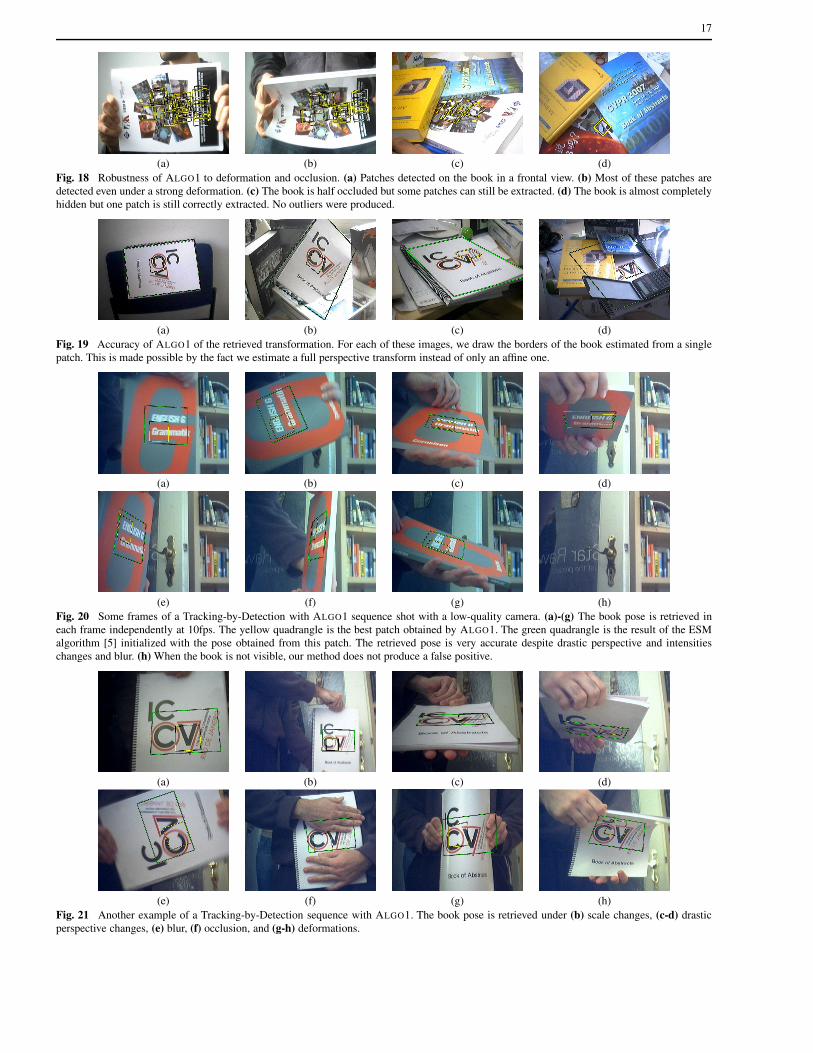
7.2 Examples

In Figs. 18, 19, 20, and 21, we apply ALGO1 to object de-

tection and pose estimation application using a low-quality

camera. ALGO1 is robust and accurate even in presence of

drastic perspective changes, light changes, blur, occlusion,

and deformations. For each of these objects we learned the

patches from an initial frontal view. In Figs. 20 and 21 we

used the template matching-based ESM algorithm [5] to re-

fine the pose obtained from a single patch. As one can see,

one extracted patch is already good enough to obtain the

pose of the object reliably.

Several applications using ALGO2 are shown in Figs. 22,

23, 24, and 25, showing SLAM re-localisation using a single

keypoint, SLAM re-localisation in a room, poorly textured

object detection, and deformable object detection, respec-

tively.

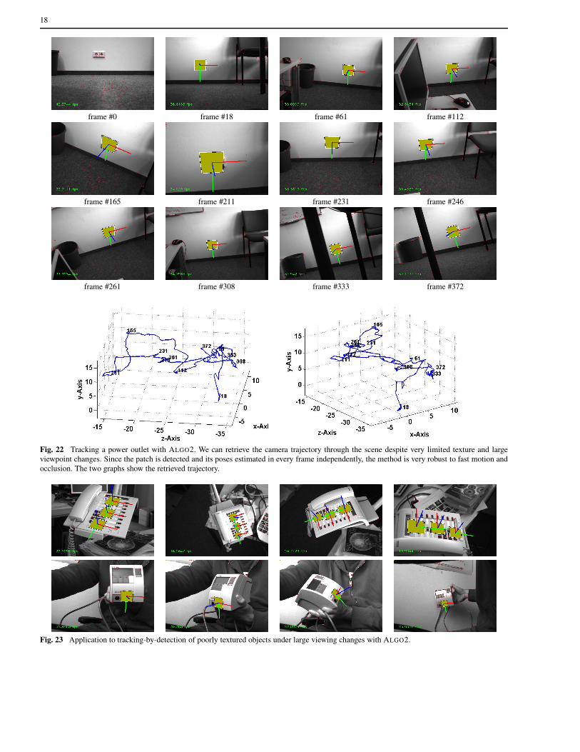
For the experiment shown Fig. 22, we considered an im-

age sequence that is typically very challenging for existing

SLAM systems as very few feature points can be detected,

and in which the camera moves very quickly. We used a

frontal view of the power outlet to train ALGO2, which was

then able to detect it and provide the camera pose throughout

the 372 images of the sequence.

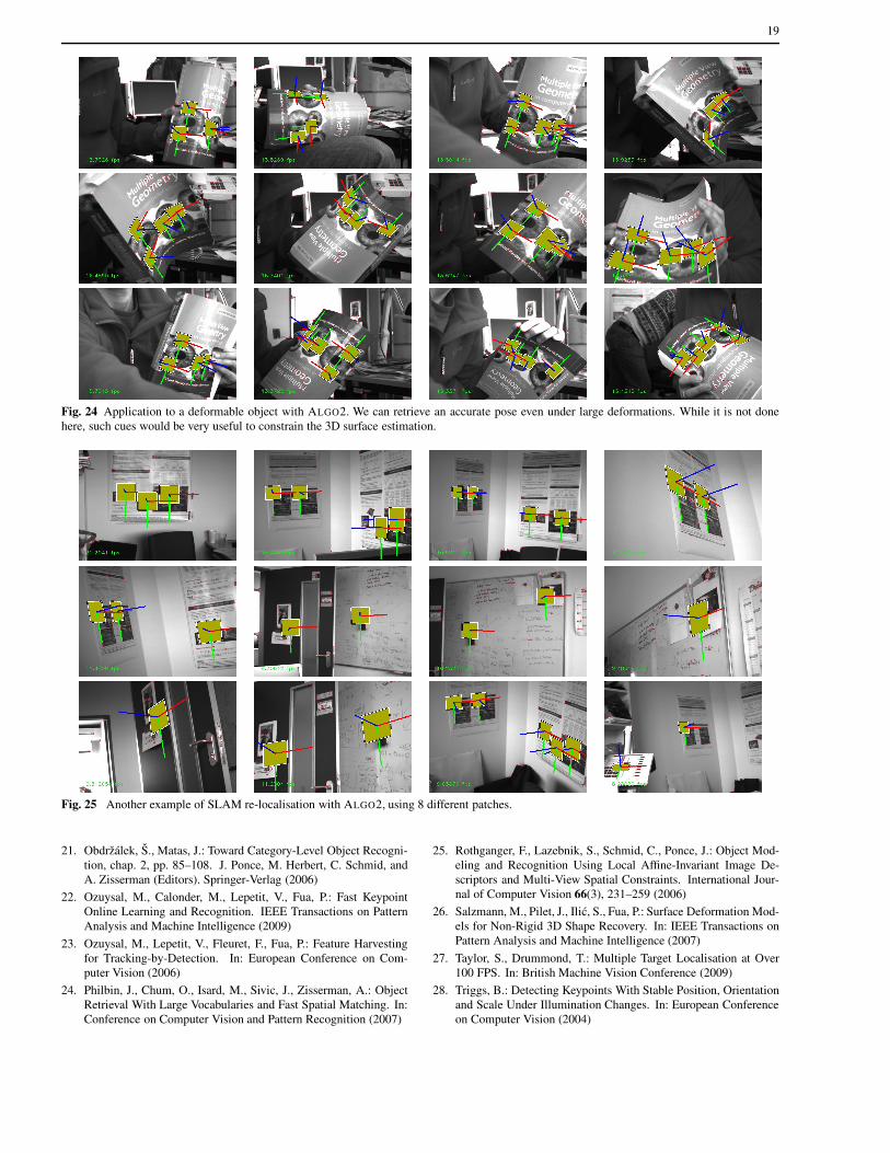
Fig. 25 shows another example on a larger scene. We

walked around an office space and learned a few key land-

marks which were then reliably redetected in the next frames

when visible, even under new viewpoints. While scalability

is an issue in our current application as we cannot handle too

many patches simultaneously, this is balanced by the fact

that each patch provides all six degrees-of-freedom of the

camera. We currently ignore the spatial relations between

patches, and the camera pose is only computed in the local

16

frame of each patch. It should however be possible to build a

SLAM system that estimates the geometric transformations

between the patches local frames and compute the camera

pose in a global coordinates system.

In Fig. 23 we applied ALGO2 to detect and estimate the

3–D pose of two poorly textured objects, under different

scales and poses. This shows the potential of our approach

for object recognition.

For Fig. 24 we tried our approach on a deformable sur-

face. We learned five patches on the book cover from an

initial frontal view. Although the book is then strongly de-

formed and we do not model the deformation within our

recognition pipeline, most of the learned patches are reliably

recognized. The local frames also fit well to the local de-

formations, at least visually. This provides very strong con-

straints on the shape of the surface that could be exploited

to retrieve the deformations, for example using a global de-

formation model such as the one developed in [26].

A clear limitation of our approach is that it relies on fea-

ture point detection. If the feature point corresponding to the

patch center is not detected in the first place, because of im-

age noise or some imperfection of the feature point detector,

our approach fails. Skipping the feature point detection step,

for example, by parsing the complete image and looking for

the patches, is part of our future work.

8 Conclusion

We showed that including pose estimation within the recog-

nition process considerably improves the robustness and the

accuracy of the results of object detection, and this makes

our approach highly desirable. Thanks to a two-step algo-

rithm, it is possible to get matching sets that do usually con-

tain no outliers. Even low-textured objects can therefore be

well detected and their pose well estimated.

We showed in the paper that a Fern based classifier is

able to recognize the keypoints in a very fast manner that

allows to track several hundred patches very accurately in

real-time. We also showed that the simultaneous estimation

of keypoint identities and poses is more reliable but slower

than the two separate steps undertaken consecutively. Fi-

nally, we showed how to build in real-time a one-way de-

scriptor based on geometric blur that quickly, robustly and

accurately estimates the pose of feature points and therefore

is appropriate for applications where real-time learning is

mandatory.

We demonstrated in various experiments the improved

performance compared to previous state-of-the-art methods

and demonstrated our approach on many applications in-

cluding simple 3D tracking-by-detection, SLAM applica-

tions, low-textured object detection and deformable objects

registration. However, many other applications could benefit

from it, such as object recognition, image retrieval or robot

localization.

Acknowledgements This project was granted partly by BMBF (AVILUS-

plus: 01IM08002) and by the Bayrische Forschungsstiftung BFS.

References

1. Baker, S., Datta, A., Kanade, T.: Parameterizing Homographies.

Tech. rep., CMU (2006)2. Baker, S., Matthews, I.: Lucas-Kanade 20 Years On: A Unifying

Framework. International Journal of Computer Vision 56(3), 221–

255 (2004)3. Bay, H., Tuytelaars, T., Van Gool, L.: SURF: Speeded Up Robust

Features. In: European Conference on Computer Vision (2006)

4. Beis, J., Lowe, D.: Shape Indexing Using Approximate Nearest-

Neighbour Search in High-Dimensional Spaces. In: Conference

on Computer Vision and Pattern Recognition, pp. 1000–1006

(1997)5. Benhimane, S., Malis, E.: Homography-Based 2D Visual Tracking

and Servoing. IJRR 26(7), 661–676 (2007)

6. Berg, A., Malik, J.: Geometric Blur for Template Matching. In:

Conference on Computer Vision and Pattern Recognition (2002)

7. B.J.Frey, Jojic, N.: Transformation Invariant Clustering Using the

EM Algorithm. IEEE Transactions on Pattern Analysis and Ma-

chine Intelligence (2003)8. Chum, O., Matas, J.: Geometric Hashing With Local Affine

Frames. In: Conference on Computer Vision and Pattern Recog-

nition, pp. 879–884 (2006)

9. Goedeme, T., Tuytelaars, T., Van Gool, L.: Fast Wide Baseline

Matching for Visual Navigation. In: Conference on Computer Vi-

sion and Pattern Recognition (2004)

10. Grabner, H., Bischof, H.: On-Line Boosting and Vision. In: Con-

ference on Computer Vision and Pattern Recognition (2006)11. Grabner, M., Grabner., H., Bischof, H.: Learning Features for

Tracking. In: Conference on Computer Vision and Pattern Recog-

nition (2007)

12. Hinterstoisser, S., Benhimane, S., Navab, N., Fua, P., Lepetit, V.:

Online Learning of Patch Perspective Rectification for Efficient

Object Detection. In: Conference on Computer Vision and Pattern

Recognition (2008)13. Hinterstoisser, S., Kutter, O., Navab, N., Fua, P., Lepetit, V.: Real-

Time Learning of Accurate Patch Rectification. In: Conference on

Computer Vision and Pattern Recognition (2009)14. Jurie, F., Dhome, M.: Hyperplane Approximation for Template

Matching. IEEE Transactions on Pattern Analysis and Machine

Intelligence 24(7), 996–100 (2002)

15. Lepetit, V., Lagger, P., Fua, P.: Randomized Trees for Real-Time

Keypoint Recognition. In: Conference on Computer Vision and

Pattern Recognition (2005)16. Lowe, D.: Distinctive Image Features from Scale-Invariant Key-

points. International Journal of Computer Vision 20(2), 91–110

(2004)

17. Matas, J., Chum, O., Martin, U., Pajdla, T.: Robust Wide Base-

line Stereo from Maximally Stable Extremal Regions. In: British

Machine Vision Conference, pp. 384–393 (2002)

18. Mikolajczyk, K., Schmid, C.: Scale and Affine Invariant Interest

Point Detectors. International Journal of Computer Vision (2004)19. Mikolajczyk, K., Tuytelaars, T., Schmid, C., Zisserman, A.,

Matas, J., Schaffalitzky, F., Kadir, T., Van Gool, L.: A Compari-

son of Affine Region Detectors. International Journal of Computer

Vision 65(1), 43–72 (2005)

20. Molton, N., Davison, A., Reid, I.: Locally Planar Patch Features

for Real-Time Structure from Motion. In: British Machine Vision

Conference (2004)

17

(a) (b) (c) (d)

Fig. 18 Robustness of ALGO1 to deformation and occlusion. (a) Patches detected on the book in a frontal view. (b) Most of these patches are

detected even under a strong deformation. (c) The book is half occluded but some patches can still be extracted. (d) The book is almost completely

hidden but one patch is still correctly extracted. No outliers were produced.

(a) (b) (c) (d)

Fig. 19 Accuracy of ALGO1 of the retrieved transformation. For each of these images, we draw the borders of the book estimated from a single

patch. This is made possible by the fact we estimate a full perspective transform instead of only an affine one.

(a) (b) (c) (d)

(e) (f) (g) (h)

Fig. 20 Some frames of a Tracking-by-Detection with ALGO1 sequence shot with a low-quality camera. (a)-(g) The book pose is retrieved in

each frame independently at 10fps. The yellow quadrangle is the best patch obtained by ALGO1. The green quadrangle is the result of the ESM

algorithm [5] initialized with the pose obtained from this patch. The retrieved pose is very accurate despite drastic perspective and intensities

changes and blur. (h) When the book is not visible, our method does not produce a false positive.

(a) (b) (c) (d)

(e) (f) (g) (h)

Fig. 21 Another example of a Tracking-by-Detection sequence with ALGO1. The book pose is retrieved under (b) scale changes, (c-d) drastic

perspective changes, (e) blur, (f) occlusion, and (g-h) deformations.

18

frame #0 frame #18 frame #61 frame #112



Fig. 22 Tracking a power outlet with ALGO2. We can retrieve the camera trajectory through the scene despite very limited texture and large

viewpoint changes. Since the patch is detected and its poses estimated in every frame independently, the method is very robust to fast motion and

occlusion. The two graphs show the retrieved trajectory.

Fig. 23 Application to tracking-by-detection of poorly textured objects under large viewing changes with ALGO2.

19

Fig. 24 Application to a deformable object with ALGO2. We can retrieve an accurate pose even under large deformations. While it is not done

here, such cues would be very useful to constrain the 3D surface estimation.

Fig. 25 Another example of SLAM re-localisation with ALGO2, using 8 different patches.

21. Obdrzalek, S., Matas, J.: Toward Category-Level Object Recogni-

tion, chap. 2, pp. 85–108. J. Ponce, M. Herbert, C. Schmid, and

A. Zisserman (Editors). Springer-Verlag (2006)

22. Ozuysal, M., Calonder, M., Lepetit, V., Fua, P.: Fast Keypoint

Online Learning and Recognition. IEEE Transactions on Pattern

Analysis and Machine Intelligence (2009)

23. Ozuysal, M., Lepetit, V., Fleuret, F., Fua, P.: Feature Harvesting

for Tracking-by-Detection. In: European Conference on Com-

puter Vision (2006)

24. Philbin, J., Chum, O., Isard, M., Sivic, J., Zisserman, A.: Object

Retrieval With Large Vocabularies and Fast Spatial Matching. In:

Conference on Computer Vision and Pattern Recognition (2007)

25. Rothganger, F., Lazebnik, S., Schmid, C., Ponce, J.: Object Mod-

eling and Recognition Using Local Affine-Invariant Image De-

scriptors and Multi-View Spatial Constraints. International Jour-

nal of Computer Vision 66(3), 231–259 (2006)

26. Salzmann, M., Pilet, J., Ilic, S., Fua, P.: Surface Deformation Mod-

els for Non-Rigid 3D Shape Recovery. In: IEEE Transactions on

Pattern Analysis and Machine Intelligence (2007)

27. Taylor, S., Drummond, T.: Multiple Target Localisation at Over

100 FPS. In: British Machine Vision Conference (2009)

28. Triggs, B.: Detecting Keypoints With Stable Position, Orientation

and Scale Under Illumination Changes. In: European Conference

on Computer Vision (2004)

20

29. Williams, B., Klein, G., Reid, I.: Real-Time SLAM Relocalisation.

In: International Conference on Computer Vision (2007)

learning real-time perspective patch rectiﬁcation · pdf filelearning real-time perspective...

Documents