learning and identifying desktop macros using an enhanced lz78 … · using an enhanced lz78...
TRANSCRIPT

Department of Computer Science and Engineering University of Texas at Arlington
Arlington, TX 76019
Learning and Identifying Desktop Macros Using an Enhanced LZ78 Algorithm
Forrest Elliott [email protected]
Technical Report CSE-2004-12
This report was also submitted as an M.S. thesis.

LEARNING AND IDENTIFYING DESKTOP MACROS USING AN
ENHANCED LZ78 ALGORITHM
The members of the Committee approve the masters
thesis of Forrest Elliott
Manfred Huber ____________________________________
Supervising Professor
Diane Cook ____________________________________
Lawrence Holder ____________________________________

Copyright © by Forrest Elliott, 2004
All Rights Reserved
LEARNING AND IDENTIFYING DESKTOP MACROS USING AN
ENHANCED LZ78 ALGORITHM
by
FORREST ELLIOTT
Presented to the Faculty of the Graduate School of
The University of Texas at Arlington in Partial Fulfillment
of the Requirements
for the Degree of
MASTER OF SCIENCE IN COMPUTER SCIENCE AND ENGINEERING
THE UNIVERSITY OF TEXAS AT ARLINGTON
December 2004

iv
ACKNOWLEDGMENTS
I would like to express my gratitude to Dr. Huber in guiding and focusing my
research over the months. Especially important, in hindsight, were hints related to creating a
system model. I would also like to thank Dr. Cook for pointing me in the right direction at
the very beginning. The direction being: approach the problem from an information theoretic
perspective. I would also like to thank Dr. Holder, and the defense committee as a whole, for
there assistance and comments.
9 November 2004
v
ABSTRACT
LEARNING AND IDENTIFYING DESKTOP MACROS USING AN
ENHANCED LZ78 ALGORITHM
Publication No. _______
Forrest Elliott, M.S.
The University of Texas at Arlington, 2004
Supervising Professor: Manfred Huber
Important to the evolution of technology is the notion of automation. One way to
increase automation for the PC user is to use macros. The current paradigm for creating
macros is for the user to record a macro and then play the macro back. This is a manual
process. In this thesis we explore a system whereby macros are learned automatically. With
an automated system macro learning can be a continuous background operation. In this way
not only can intended macros be learned but unintended useful macros can be learned as
well. Once a macro is learned it can be offered back to the user for playback at opportune
times. Central to this macro learning system is the Lempel-Ziv algorithm which was
originally developed for data compression. In this thesis we enhance the algorithm for
improved performance from a learning perspective. With the enhanced algorithm it is

vi
possible for a macro to be learned and offered back to the user in as few as three exposures to
a sequence. Actual implementation experiments bear out this capability.
vii
TABLE OF CONTENTS
ACKNOWLEDGMENTS .................................................................................................. iv
ABSTRACT ........................................................................................................................ v
LIST OF FIGURES ............................................................................................................ x
LIST OF TABLES .............................................................................................................. xii
Chapter
1. INTRODUCTION ......................................................................................................... 1
1.1 World Wide Web ............................................................................................. 2
1.2 Macros ............................................................................................................. 4
1.3 Sequence Learning ........................................................................................... 5
1.4 Chapter Organization ....................................................................................... 6
2. MACRO SYSTEM DESIGN ........................................................................................ 7
2.1 Related Work ................................................................................................... 7
2.2 Description ....................................................................................................... 10
2.3 Components ..................................................................................................... 11
2.4 Operating System Interface ............................................................................. 12
3. LEMPEL-ZIV ALGORITHM ....................................................................................... 15
3.1 Related Work ................................................................................................... 15
3.2 Lempel-Ziv Model ........................................................................................... 17
3.3 LZ78 Example ................................................................................................. 18
4. ENHANCED LEMPEL-ZIV ALGORITHM ................................................................ 22
4.1 Three Enhancement Rules ............................................................................... 22

viii
4.1.1 Next Node Pointer ............................................................................ 23
4.1.2 Next Node Duplication ..................................................................... 25
4.1.3 Continue When Duplicating Nodes .................................................. 26
4.2 Side Effects ...................................................................................................... 27
4.3 Learning ........................................................................................................... 28
4.4 Compression and Decompression .................................................................... 30
5. ENHANCED LZ78 AND MACRO RECORDING ...................................................... 32
5.1 User Action Symbols ....................................................................................... 33
5.2 Prediction by Partial Match (PPM) .................................................................. 37
5.3 Macro Start Point ............................................................................................. 39
5.4 Macro End Point .............................................................................................. 41
5.5 Symbol vs. Sequence Probabilities .................................................................. 44
5.6 Macro Utility .................................................................................................... 47
5.7 Example Situations .......................................................................................... 48
5.7.1 Common Prefix Macros .................................................................... 49
5.7.2 Substring Macros .............................................................................. 50
5.7.3 Macro with Noise .............................................................................. 51
6. PERFORMANCE STUDY ............................................................................................ 53
6.1 Representative Scenario ................................................................................... 53
6.1.1 Number of Tree Nodes ...................................................................... 58
6.1.2 Compression ..................................................................................... 59
6.1.3 Macro Subsuming ............................................................................. 62
6.2 Noise Substring Scenario ................................................................................. 63
6.2.1 Utility Threshold Effects ................................................................... 64
6.2.2 Utility Cost Effects ............................................................................ 66

ix
6.3 Human Data Experiment .................................................................................. 69
6.3.1 Analysis ............................................................................................ 73
6.3.2 Generic Problems .............................................................................. 75
7. CONCLUSIONS ............................................................................................................ 77
BIBLIOGRAPHY ............................................................................................................... 79
BIOGRAPHICAL STATEMENT ...................................................................................... 81
x
LIST OF FIGURES
Figure Page
1 User Navigation Domains .............................................................................. 3
2 System Components ....................................................................................... 11
3 Journal Record Hook Point ............................................................................ 13
4 Dictionary Compression Model ..................................................................... 18
5 LZ78 Dictionary for Sequence “AABABC” ................................................. 20
6 LZ78 Dictionary for Sequence “ABCABBCCD” ......................................... 20
7 Loss of Context Information .......................................................................... 24
8 No Loss of Context Information .................................................................... 24
9 Next Node Pointers for Sequence “ABC” ..................................................... 25
10 Sequence “ABCAB” ...................................................................................... 26
11 Sequence “ABCABC” ................................................................................... 27
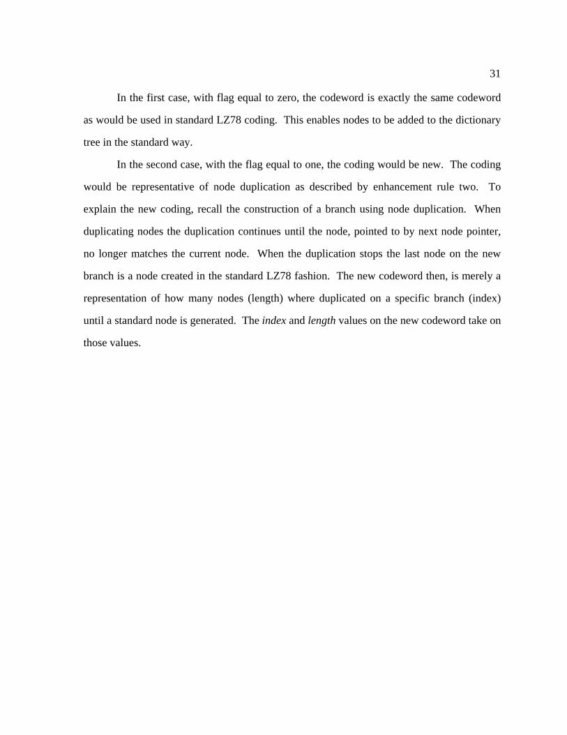
12 Macro in LZ78 Dictionary Tree ..................................................................... 33
13 Macro M with Prefixing Symbols X and Y ................................................... 40
14 Macro M with No Prefixing Symbol ............................................................. 40
15 Last Symbol Test ........................................................................................... 42
16 Macro End Point Identification ...................................................................... 42
17 Symbol Counting vs. Sequence Counting ..................................................... 43
18 Macros with Common Prefix Symbol ........................................................... 50
19 Two Macros, One a Substring of the Other .................................................... 51
20 Macro with Less Frequent Noise-like Substrings .......................................... 52

xi
21 Four Symbol Dictionary Tree Comparison .................................................... 59
22 Approximate Compression for 27 Exposures ................................................ 61
23 Approximate Compression for 500 Exposures .............................................. 61
24 Human Data Experiment Results ................................................................... 71
25 Incremental Human Data Predictions for Trial One through Trial Eight ...... 72
xii
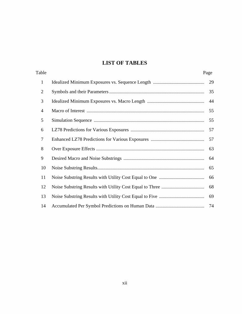
LIST OF TABLES
Table Page
1 Idealized Minimum Exposures vs. Sequence Length ........................................... 29
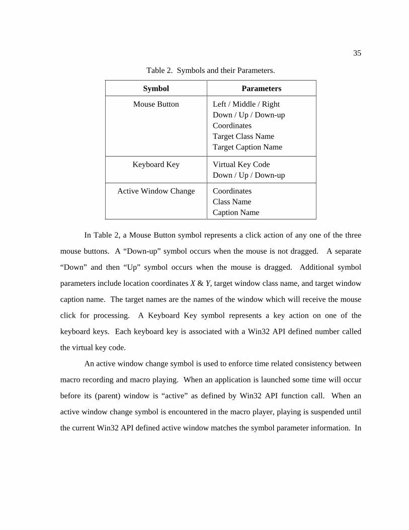
2 Symbols and their Parameters ................................................................................ 35
3 Idealized Minimum Exposures vs. Macro Length ................................................ 44
4 Macro of Interest ................................................................................................... 55
5 Simulation Sequence ............................................................................................. 55
6 LZ78 Predictions for Various Exposures .............................................................. 57
7 Enhanced LZ78 Predictions for Various Exposures ............................................. 57
8 Over Exposure Effects ........................................................................................... 63
9 Desired Macro and Noise Substrings .................................................................... 64
10 Noise Substring Results.......................................................................................... 65
11 Noise Substring Results with Utility Cost Equal to One ...................................... 66
12 Noise Substring Results with Utility Cost Equal to Three .................................... 68
13 Noise Substring Results with Utility Cost Equal to Five ...................................... 69
14 Accumulated Per Symbol Predictions on Human Data ......................................... 74

1
CHAPTER 1
INTRODUCTION
The current personal computer (PC) desktop environment paradigm consists of a
variety of applications running on a single operating system. Each application is designed to
enable specific user tasks and goals to be achieved. During the application development
stage, the programmer will envision an arrangement of windows, sub windows, and buttons
that will allow the user to achieve his goals. For example “file print number of copies
5 ok” is “windows-speak” for the sequence of button clicks needed to achieve a user
goal of printing five copies.
Larger, more powerful applications typically have a very large number of buttons.
Some buttons can be seen when an application is started. Examples of these include “menu”
buttons and “toolbar” buttons. Other buttons are not visible and can only be accessed by first
clicking a menu or toolbar button. As a result of this sort of design complexity, the range
and depth of possible click sequences becomes extremely large.
Hidden in the application’s design are the button click sequences a user is required to
learn in order to make a program function. The sequences are learned by the user over time
through a process of discovery. A user who is more experienced with an application in
essence has learned more button sequences. Naturally, all users start out with zero specific
knowledge of how a program is used.
In this thesis we create a program that monitors the sequences performed by the user.
As the user discovers and learns button sequences, so does the monitoring program. Ideally
the monitoring program is always running so that all the sequences discovered by the user

2
are simultaneously learned by the monitoring program. Such a monitoring program is
described here as a macro recorder.
1.1 World Wide Web
The World Wide Web (WWW) paradigm is similar to the desktop paradigm. In the
WWW environment a user clicks Web page hyperlinks until the information the user seeks is
found. Clicking through a sequence of hyperlinks is similar to clicking through a sequence
of application buttons. The usefulness of learning user sequences is different for Web
navigation though. In the desktop environment the user benefits from the learned sequence
of button clicks. The user has learned how to use a program. In the Web environment an
Internet search engine can benefit. The search engine can improve the quality of the links
returned from a search. If a search engine monitors and learns which pages are actually
being examined from a query it can re-rank those pages higher on all subsequent identical
queries. Internet search engine technology, and the quality of hyperlinks returned, is a
significant area of research.
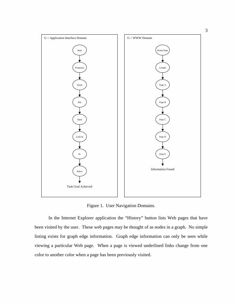
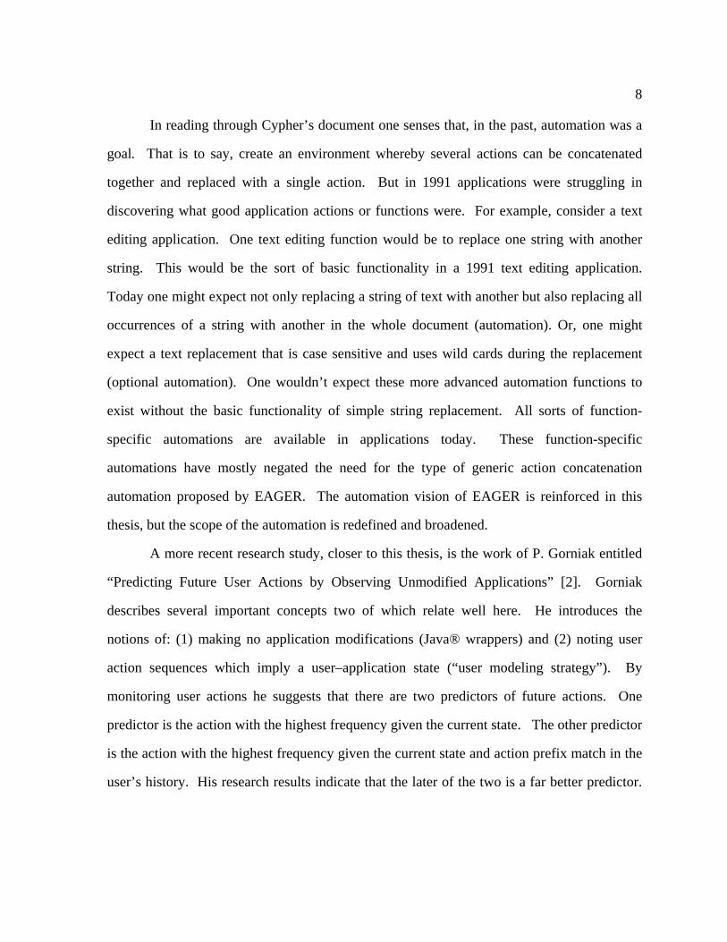
It is interesting to correlate graphs induced by user navigation in an application with
graphs induced by user navigation on the Web. In this comparison we can see that graph
nodes are buttons in the application domain and graph nodes are HTML formatted pages in
the WWW domain. Graph edges can be correlated as well. In the application domain graph
edges are navigation paths used to achieve a goal or task. In the WWW domain graph edges
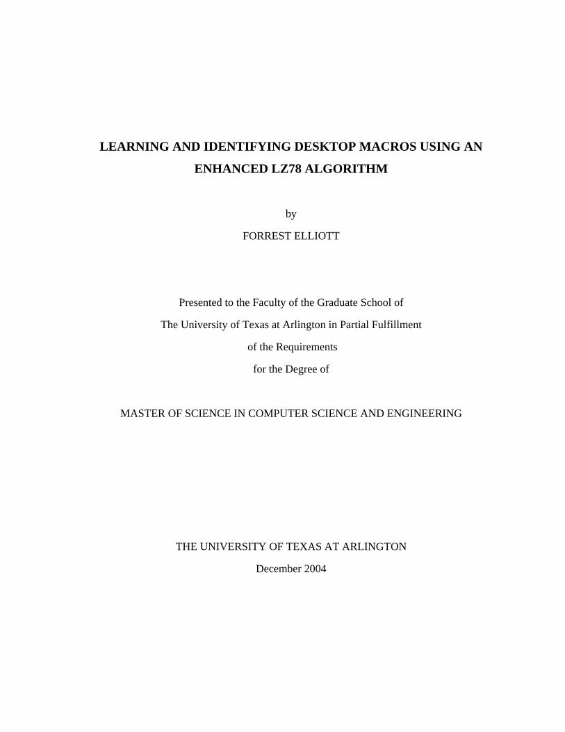
are navigation paths used to find desired information. Figure 1 shows an example.
3
Figure 1. User Navigation Domains.
In the Internet Explorer application the “History” button lists Web pages that have
been visited by the user. These web pages may be thought of as nodes in a graph. No simple
listing exists for graph edge information. Graph edge information can only be seen while
viewing a particular Web page. When a page is viewed underlined links change from one
color to another color when a page has been previously visited.
G = Application Interface Domain
Start
Programs
Word
File
Open
Look In
D:
Select
Home Page
Page A
Page B
Page C
Page D
Page E
Information Found
Task Goal Achieved
G = WWW Domain

4
Learning user navigational paths, and thinking of them in terms of a graph, seems
appropriate in both the application interface domain and the WWW search domain. In the
application interface domain the user clicks hundreds, or perhaps even thousands, of times on
various applications. In the WWW domain identical search queries, and the Web page
ultimately traveled to, could be a fairly common occurrence. Given a large enough
population of searches one could expect an association to be learned. The model used in
learning macros might be a model similar to the one used for learning search results. If so
then improving the ranking of search results should be possible. In both cases prodigious
amounts of input data can be expected to produce only a limited number of relations.
Besides the difference in who benefits for the two cases, another difference would be where
the learning algorithm would be located. The learning algorithm resides on a PC in the
macro learning case and the learning algorithm resides on a search engine in the second case.
1.2 Macros
The term used to describe a single user action, which automates a series of user
actions, is “macro”. The terminology used in creating and using a macro is borrowed from
the terminology used in audio tape recorders. Both involve sequences in time. To create a
macro, a macro is “recorded”. To use a macro, a macro is “played”. A macro may be played
back any number of times and at the discretion of the user. One would operate a macro
recorder just as one would operate a tape recorder.
Some of the more powerful applications, such as Computer Aided Design (CAD)
programs, will normally include some sort of macro record and play functionality.
Engineering often requires the designer to replicate certain facets or pieces of a design. The
designer must therefore iterate a series of mouse or keyboard actions for each replicated
design piece. Macro functionality in a CAD environment speeds development by automating
5
laborious actions. Unfortunately though, macro functionality is confined to the CAD
application. The CAD application only has visibility to its own state and it can only initiate
actions on itself.
1.3 Sequence Learning
Since macros are ordered sequences of user actions, the problem of learning a macro
becomes learning a sequence of user actions. In a typical macro recorder the user is provided
with record, stop and play buttons. With manual macro recording, start and stop buttons
clearly demark when the macro recording starts and stops. But when the sequence is not
delimited by a stop and start command and is embedded somewhere in the users history the
problem becomes more difficult. The macro sequence must be implied based on the
historical evidence. The problem can be made more tractable though by asserting that a
macro can be characterized as a sequence of actions that have repeated in the past. The
intuition to this characterization will develop from a graphical representation and the
Lempel-Ziv algorithm.
The Lempel-Ziv algorithm, in a nut shell, allows us to find repeating sequences in
source data. The problem with the algorithm though is that the algorithm learns slowly. A
brute-force method could be used to identify sequences with fewer user sequence exposures
but the computational overhead of searching all or most of the user’s history on every user
action is prohibitive. The Lempel-Ziv algorithm enables us to find repeating sequences with
much lower overhead. In this thesis we formulate a modification to the algorithm which has
the potential of learning sequences in far fewer sequence exposures. The enhanced algorithm
can learn a sequence in as few as two sequence exposures and the sequence end point can be
identified on the third sequence exposure. On subsequent sequence exposures the learned

6
sequence can be offered to the user for play. Tests of the algorithm implemented on a PC
bears out this capability.
1.4 Chapter Organization
The overall system design, including the operating system record hook and macro
player, is described in chapter 2. The Lempel-Ziv algorithm is described in chapter 3.
Enhancements to the Lempel-Ziv algorithm are described in chapter 4. The details required
to characterize, learn, and predict macros are given in chapter 5. In chapter 6 a macro
learning experiment is performed and the Lempel-Ziv algorithm’s learning rate is compared
to the enhanced Lempel-Ziv algorithm’s learning rate. Also in chapter 6 is a human data
experiment where fellow students created their own macros.
7
CHAPTER 2
MACRO SYSTEM DESIGN
2.1 Related Work
The concept of manual macro recording and playback, using a start and stop button,
is very straight forward. No significant research work exists which is confined to this single
topic. Other areas of functionality, related to macros and close to the ideas presented here,
have been a focus of research in the past. One type of research is “programming by
example”. Other variants exist such as “programming by demonstration” and “macro by
example”. All of these subjects are more involved and less straight forward then merely
recording and playing macros.
In programming by example user actions are monitored. When a pattern is detected,
a script-like program is generated which will automate and complete the remaining actions.
The user may then invoke the script to complete the task. A significant earlier work in
programming by example is the system proposed by A. Cypher in 1991 which he calls
“EAGER: Programming Repetitive Tasks by Example” [1]. In his scenario description, the
application is email and the task is creating a list of received email message subjects. As the
user interacts with the application, the EAGER system detects when an action or button
sequence is duplicated twice in a row. On the third iteration the system highlights the
buttons it believes the user will activate next. Highlighted buttons show the user that
EAGER has identified a sequence of actions. Then at the beginning of the fourth iteration a
special icon pops up. The icon is a graphic of a mouse. Clicking the icon causes EAGER to
perform the action sequence learned in the previous iterations.
8
In reading through Cypher’s document one senses that, in the past, automation was a
goal. That is to say, create an environment whereby several actions can be concatenated
together and replaced with a single action. But in 1991 applications were struggling in
discovering what good application actions or functions were. For example, consider a text
editing application. One text editing function would be to replace one string with another
string. This would be the sort of basic functionality in a 1991 text editing application.
Today one might expect not only replacing a string of text with another but also replacing all
occurrences of a string with another in the whole document (automation). Or, one might
expect a text replacement that is case sensitive and uses wild cards during the replacement
(optional automation). One wouldn’t expect these more advanced automation functions to
exist without the basic functionality of simple string replacement. All sorts of function-
specific automations are available in applications today. These function-specific
automations have mostly negated the need for the type of generic action concatenation
automation proposed by EAGER. The automation vision of EAGER is reinforced in this
thesis, but the scope of the automation is redefined and broadened.
A more recent research study, closer to this thesis, is the work of P. Gorniak entitled
“Predicting Future User Actions by Observing Unmodified Applications” [2]. Gorniak
describes several important concepts two of which relate well here. He introduces the
notions of: (1) making no application modifications (Java® wrappers) and (2) noting user
action sequences which imply a user–application state (“user modeling strategy”). By
monitoring user actions he suggests that there are two predictors of future actions. One
predictor is the action with the highest frequency given the current state. The other predictor
is the action with the highest frequency given the current state and action prefix match in the
user’s history. His research results indicate that the later of the two is a far better predictor.
9
Although Gorniak’s action prediction concepts are fundamental, he fails to establish an
algorithmic model.
Historically it should be mentioned that P. Gorniak’s work is built on B. Davison’s
work. Davison’s work is titled “Predicting Sequences of User Actions” [3]. He describes
predicting user actions based on the “… Markov assumption that each command depends
only on the previous command (i.e., patterns of length two, so that the previous command is
the state)”. Davison experimented with this notion by integrating a command prediction
scheme into the UNIX® shell [4]. Gorniak extended Davison’s prediction idea with the
notion that the previous several commands can be used to identify the current state.
A couple of previous works geared specifically to macro generation include A.
Sugiura “Simplifying Macro Definition in Programming by Automation” [5] and D.
Kurlander “A history-based macro by example system” [6]. In Sugiura’s paper he advocates
the convenience of continuously recording user actions. In effect the macro recorder is
always on. This relieves the user from manually turning on and off the recording as is
required with a normal tape recorder. His system fails to circumvent the application domain
problem though. The described macro functionality only works inside the described
application: “DemoOffice”. By working inside the DemoOffice application, the start and
end points of a macro may be inferred from action side effects; which he calls “action
slicing”.
D. Kurlander’s [6] work is more Graphical User Interface (GUI) based. Kurlander
recognizes the need for the user to be able to visualize what effects a macro will have if
executed. He describes an application called “Chimera”. Chimera allows the user to view
his history of actions in a coalesced graphical form. The coalesced actions are viewed as a
sequence of frames or pictures. With this graphical presentation a Chimera user can edit and
build a macro similar to the way a video clip is created. This thesis espouses to automate the
10
macro creation process via learning rather than leaving the process to the user. Kurlander’s
work does suggest an idea not incorporated here. User mouse button click actions could be
compared with much greater precision if the graphics underneath the mouse pointer was
included in the comparison. This thesis does not extend to this area.
2.2 Description
This thesis proposes that by learning user actions as macros, PC desktop automation
can take a new step; a step up to a higher level of automation. That is, instead of learning
tasks within a single application, learn tasks on a broader scope. Learn tasks as macros at the
PC desktop level. Macros available anywhere on the desktop allow a user to attain higher
levels of efficiency and productivity. They allow the user to automate the entire range of
user work actions. For example, a macro could consist of a series of actions spread across
several applications.
The first question becomes how can macros be learned at the desktop level? Adding
a new application in a normal fashion would not solve the problem. Applications are not
inherently given visibility to button and mouse click actions occurring in other applications
running on the desktop. For security reasons the Operating System (OS) limits application
visibility. The OS inherently confines visibility of an application to itself, its offspring, and
to the public resources provided by the OS.
One way to gain visibility to all running desktop applications is to attach to the
operating system. By integrating into the OS a macro recording application can gain
additional security rights and therefore additional visibility. Such an integrated macro
recording application would have visibility to all running desktop applications. This is the
approach taken here.
11
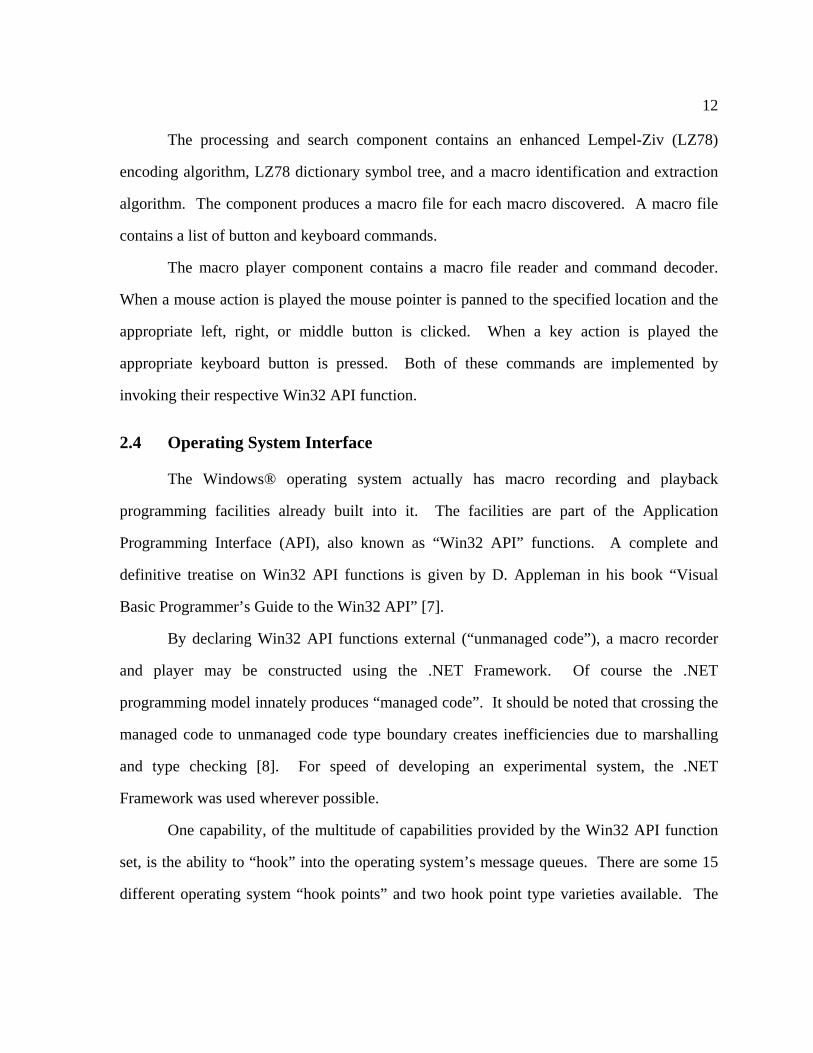
2.3 Components
A system capable of learning user habits and providing automation of the desktop
would include:
1. Mouse button and keyboard key recorder
2. Learning algorithm
3. Button and key player
A top level diagram of the system components and their interconnections is shown in
Figure 2.
Figure 2. System Components.
The history recorder component contains an operating system “hook” procedure to
capture and record user keyboard and mouse actions. The procedure writes the list of actions
to a file for preservation.
History Recorder Macro Player
Operating
System
Record
Hook
User
Mouse
Button
Actions
User
Keyboard
Key
Actions
Play
Actions
History
File
Processing and Search
Mouse
Button
CommandsLZ78
Encode
Parse
Keyboard
Key
Commands
Macro
Files
Macro
Identification
LZ78
Dictionary
Context (last few actions)
12
The processing and search component contains an enhanced Lempel-Ziv (LZ78)
encoding algorithm, LZ78 dictionary symbol tree, and a macro identification and extraction
algorithm. The component produces a macro file for each macro discovered. A macro file
contains a list of button and keyboard commands.
The macro player component contains a macro file reader and command decoder.
When a mouse action is played the mouse pointer is panned to the specified location and the
appropriate left, right, or middle button is clicked. When a key action is played the
appropriate keyboard button is pressed. Both of these commands are implemented by
invoking their respective Win32 API function.
2.4 Operating System Interface
The Windows® operating system actually has macro recording and playback
programming facilities already built into it. The facilities are part of the Application
Programming Interface (API), also known as “Win32 API” functions. A complete and
definitive treatise on Win32 API functions is given by D. Appleman in his book “Visual
Basic Programmer’s Guide to the Win32 API” [7].
By declaring Win32 API functions external (“unmanaged code”), a macro recorder
and player may be constructed using the .NET Framework. Of course the .NET
programming model innately produces “managed code”. It should be noted that crossing the
managed code to unmanaged code type boundary creates inefficiencies due to marshalling
and type checking [8]. For speed of developing an experimental system, the .NET
Framework was used wherever possible.
One capability, of the multitude of capabilities provided by the Win32 API function
set, is the ability to “hook” into the operating system’s message queues. There are some 15
different operating system “hook points” and two hook point type varieties available. The
13
two type varieties are: (1) local or process level and (2) global or operating system level. To
hook into all mouse and keyboard actions at the desktop level a global hook is needed. S.
Teilhet describes the gamut of hooks and how to use them in detail in his book “Subclassing
& Hooking with Visual Basic” [9].
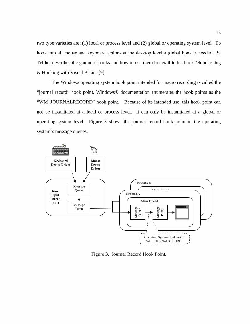
The Windows operating system hook point intended for macro recording is called the
“journal record” hook point. Windows® documentation enumerates the hook points as the
“WM_JOURNALRECORD” hook point. Because of its intended use, this hook point can
not be instantiated at a local or process level. It can only be instantiated at a global or
operating system level. Figure 3 shows the journal record hook point in the operating
system’s message queues.
Figure 3. Journal Record Hook Point.
Process B
Mes
sag
e
Qu
eue
Main Thread
Mes
sag
e
Pu
mp
Keyboard
Device Driver
Mouse
Device
Driver
Message
Queue
Message
Pump
Raw
Input
Thread
(RIT)
Process A
Mes
sag
e
Qu
eue
Main Thread
Mes
sag
e
Pu
mp
Operating System Hook Point
WH JOURNALRECORD

14
Note from Figure 3 that a mouse and keyboard journal record hook point occurs for
each process. But it must also be realized that the operating system can only have one
process running at a time. Therefore as the operating system iterates through processes to
give processing time to (multitasking) the running process’s “Message Pump” will pass
mouse and keyboard messages to the single journal record hook procedure. With this design
the order of mouse and keyboard actions can be identically preserved between:
1. Each process
2. The operating system
3. The journal record hook procedure
With a macro recording system defined the next question becomes: what is an
appropriate learning model or learning algorithm?
15
CHAPTER 3
LEMPEL-ZIV ALGORITHM
Choosing an appropriate learning algorithm is important. Clearly if user actions are
being monitored and listed the problem of learning becomes identifying macros in that list.
The expectation would be that the more examples of a given macro there are in the list the
greater the evidence should be to resolve and define its characteristics. Some
characterizations include: where in the list does the macro start, where does it end, and what
preceding actions are occurring to expect the macro to occur next. The preceding actions are
known as “context”. When the context associated with a macro occurs, the macro can be
predicted. The terminology that will be used here is that a sequence of user actions is a
macro and the actions which precede the macro are the macro’s context.
3.1 Related Work
A landmark contribution to sequential prediction models was provided by M. Feder
in his “Universal Prediction of Individual Sequences” [10]. In his paper he shows that
predictability can be described in terms of compressibility. In particular he shows that the
Lempel-Ziv (LZ78) incremental parsing algorithm [11] in effect becomes a sequence
predictor in the long term.
As an outgrowth of the Lempel-Ziv algorithm a whole class of compression schemes
known as finite-context models (as opposed to finite-state or Markov models) has grown.
Finite context modeling schemes are described by T. Bell [12] as those where “… the last
few characters are used to condition the probability distribution for the next one”. These last
few characters are the central theme behind the Prediction by Partial Match (PPM)
16
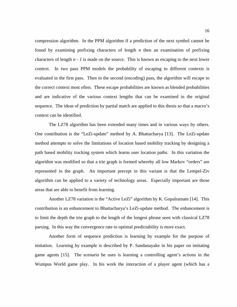
compression algorithm. In the PPM algorithm if a prediction of the next symbol cannot be
found by examining prefixing characters of length n then an examination of prefixing
characters of length n - 1 is made on the source. This is known as escaping to the next lower
context. In two pass PPM models the probability of escaping to different contexts is
evaluated in the first pass. Then in the second (encoding) pass, the algorithm will escape to
the correct context most often. These escape probabilities are known as blended probabilities
and are indicative of the various context lengths that can be examined in the original
sequence. The ideas of prediction by partial match are applied to this thesis so that a macro’s
context can be identified.
The LZ78 algorithm has been extended many times and in various ways by others.
One contribution is the “LeZi-update” method by A. Bhattacharya [13]. The LeZi-update
method attempts to solve the limitations of location based mobility tracking by designing a
path based mobility tracking system which learns user location paths. In this variation the
algorithm was modified so that a trie graph is formed whereby all low Markov “orders” are
represented in the graph. An important precept in this variant is that the Lempel-Ziv
algorithm can be applied to a variety of technology areas. Especially important are those
areas that are able to benefit from learning.
Another LZ78 variation is the “Active LeZi” algorithm by K. Gopalratnam [14]. This
contribution is an enhancement to Bhattacharya’s LeZi-update method. The enhancement is
to limit the depth the trie graph to the length of the longest phrase seen with classical LZ78
parsing. In this way the convergence rate to optimal predictability is more exact.
Another form of sequence prediction is learning by example for the purpose of
imitation. Learning by example is described by P. Sandanayake in his paper on imitating
game agents [15]. The scenario he uses is learning a controlling agent’s actions in the
Wumpus World game play. In his work the interaction of a player agent (which has a

17
playing policy) with the Wumpus World game is monitored for thousands of games. The
intent is to extract the agent’s play strategy. Once extracted, the agent’s policy can then be
compared to the policy learned by the monitoring algorithm. If they match then the imitation
of the agent has been successful. This same sort of imitation and comparison is behind the
“Turing Test” [16]. Imitation is precisely the intent behind identifying and extracting
macros.
As a side note, learning for imitation has other important advantages. An adaptable
system could be created. Such a system would consist of a sequence learning module and an
adapter. The adapter would be environment dependent and interface the scenario at hand to
the learning module. Since the learning module is independent of the environment it can be
highly optimized and generic. In P. Sandanayake’s paper, the environment is the Wumpus
World game. In this thesis, the environment is a personal computer and the actions to be
learned for imitation are the user’s actions. Although not explored here, the described macro
learning system should apply equally well to other PC environments such as Linux. A core
learning module could be developed and various adapters built for the system at hand.
3.2 Lempel-Ziv Model
The Lempel-Ziv 1978 (LZ78) algorithm is a lossless, adaptive dictionary,
compression scheme. The technique is capable of exactly reproducing the original data after
encoding and decoding with no loss of data. In an adaptive dictionary compression scheme
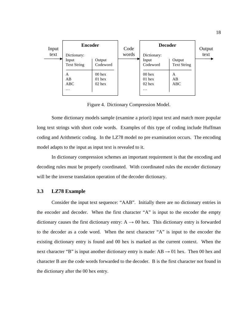
text is translated into dictionary entries and vice versa. See Figure 4.
18
Figure 4. Dictionary Compression Model.
Some dictionary models sample (examine a priori) input text and match more popular
long text strings with short code words. Examples of this type of coding include Huffman
coding and Arithmetic coding. In the LZ78 model no pre examination occurs. The encoding
model adapts to the input as input text is revealed to it.
In dictionary compression schemes an important requirement is that the encoding and
decoding rules must be properly coordinated. With coordinated rules the encoder dictionary
will be the inverse translation operation of the decoder dictionary.
3.3 LZ78 Example
Consider the input text sequence: “AAB”. Initially there are no dictionary entries in
the encoder and decoder. When the first character “A” is input to the encoder the empty
dictionary causes the first dictionary entry: A 00 hex. This dictionary entry is forwarded
to the decoder as a code word. When the next character “A” is input to the encoder the
existing dictionary entry is found and 00 hex is marked as the current context. When the
next character “B” is input another dictionary entry is made: AB 01 hex. Then 00 hex and
character B are the code words forwarded to the decoder. B is the first character not found in
the dictionary after the 00 hex entry.
Input
text
Output
text
Code
words
Encoder
Dictionary:
Input Output
Text String Codeword
A 00 hex
AB 01 hex
ABC 02 hex
…
Decoder
Dictionary:
Input Output
Codeword Text String
00 hex A
01 hex AB
02 hex ABC
…
19
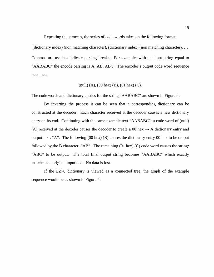
Repeating this process, the series of code words takes on the following format:
(dictionary index) (non matching character), (dictionary index) (non matching character), …
Commas are used to indicate parsing breaks. For example, with an input string equal to
“AABABC” the encode parsing is A, AB, ABC. The encoder’s output code word sequence
becomes:
(null) (A), (00 hex) (B), (01 hex) (C).
The code words and dictionary entries for the string “AABABC” are shown in Figure 4.
By inverting the process it can be seen that a corresponding dictionary can be
constructed at the decoder. Each character received at the decoder causes a new dictionary
entry on its end. Continuing with the same example text “AABABC”; a code word of (null)
(A) received at the decoder causes the decoder to create a 00 hex A dictionary entry and
output text: “A”. The following (00 hex) (B) causes the dictionary entry 00 hex to be output
followed by the B character: “AB”. The remaining (01 hex) (C) code word causes the string:
“ABC” to be output. The total final output string becomes “AABABC” which exactly
matches the original input text. No data is lost.
If the LZ78 dictionary is viewed as a connected tree, the graph of the example
sequence would be as shown in Figure 5.
20
Figure 5. LZ78 Dictionary for Sequence “AABABC”.
Starting from the root node and traveling to node A represents the 00 hex dictionary
entry. Traveling from the root node to node B represents the 01 hex dictionary entry.
Finally, traveling from the root to node C represents the 02 hex dictionary entry. These three
paths enumerate all dictionary entries for this example.
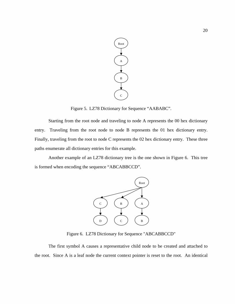
Another example of an LZ78 dictionary tree is the one shown in Figure 6. This tree
is formed when encoding the sequence “ABCABBCCD”.
Figure 6. LZ78 Dictionary for Sequence "ABCABBCCD"
The first symbol A causes a representative child node to be created and attached to
the root. Since A is a leaf node the current context pointer is reset to the root. An identical
Root
ABC
BCD
Root
A
B
C
21
process occurs for input symbols B and C. They too are added as children to the root. Each
added node is a leaf node so the current context pointer resets on each addition.
The next A (“ABCA”) causes the current context to point to node A. No nodes are
added. The next B (“ABCAB”) causes a representative B node to be created and attached to
node A. At this point the current context pointer is reset to the root. An identical process
occurs for the remaining input text BC and CD. The final dictionary parsing is: A, B, C, AB,
BC, CD.
A consequence of LZ78 parsing is that all new nodes are leaf nodes. From the
discussion above we can see that leaf nodes always reset the current context pointer to the
root. Can a leaf node be created without resetting the current context pointer? This is a
significant aspect to the enhanced LZ78 algorithm which is presented next.
22
CHAPTER 4
ENHANCED LEMPEL-ZIV ALGORITHM
One disadvantage of the LZ78 algorithm, or for that matter any of the finite-context
methods, is that it converges slowly when used for predicting. The LZ78 algorithm is a good
sequence predictor only after having been exposed to a long input sample. One could say
that the algorithm learns slowly or that it has a poor learning rate.
4.1 Three Enhancement Rules
The LZ78 enhancement presented here is a learning rate enhancement. Although
LZ78 is a greedy algorithm for learning, the changes presented here turn up the greedy
characteristic to an even higher level. Basically, a statement of the new greed is that: the first
exposure of a string of symbols is the one that should be learned. The goal is to minimize the
number of occurrences required to learn a repeating sequence. So, how can this be done and
what are the side effects?
Recall the construction of the dictionary tree as input text is revealed. A tree branch
is followed until a non-matching character occurs. At this time a new leaf is appended to the
end of the current branch or context. The addition of a leaf causes the current context pointer
to reset or start over at the root. Note that it is this action, resetting the current context
pointer, which causes a loss of sequence or context information.
To address the loss of context issue and increase the learning rate of the Lempel-Ziv
dictionary algorithm, three additional new rules are presented.
23
1. Add a “next node” pointer that represents the next character in the original
sequence.
2. When about to add a new leaf to an existing branch – check the next node pointer.
If the character that the next node pointer points to matches the input character
then duplicate the next node where the new leaf would normally be added.
3. When a duplicate leaf is appended (as outlined in 2), let the current context node
pointer continue on from the duplicate leaf instead of resetting the pointer to the
root.
As a result of rule three and given the right situation, the enhanced LZ78 algorithm
will add a leaf node without resetting the current context pointer to the root. When the
context pointer is not reset context information is not lost. Also by duplicating existing
nodes, and their next node pointers, the learning rate is improved.
4.1.1 Next Node Pointer
Recall the LZ78 dictionary tree structure. Each pointer from parent node to child
node represents exactly one piece of context information. In the sequence “ABC”, for
example, one piece of context information would be that when A occurs, B follows. Another
piece would be that when B occurs, C follows. The LZ78 dictionary tree representation is a
pointer from node A to node B and a pointer from node B to node C.
From a context perspective the worst case tree construction scenario is when all
context information is thrown away. This situation occurs when the input symbols have
never been seen before and are occurring for the first time. An example is the sequence
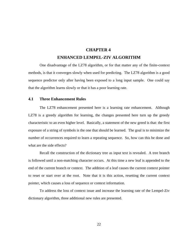
“ABC” and is shown in Figure 7. Each added node is a leaf and a leaf addition causes the
24
current context pointer to reset to the root. When the current context pointer resets all
previous sequence information (the context) is lost.
Figure 7. Loss of Context Information.
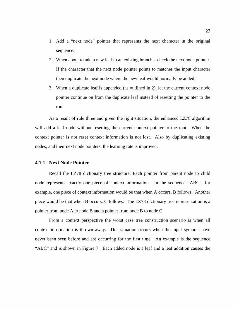
On the other hand no loss of context information occurs when the character sequence
AB is already in the dictionary tree, the current context is B, and character C is received
next. In this case character C is merely appended onto character B. See Figure 8. This is the
best case scenario for dictionary tree construction as the context of C is retained.
Figure 8. No Loss of Context Information.
The “next node pointer” concept is to create a situation whereby the dictionary tree
construction can progress from Figure 7 to Figure 8 on the second exposure to an identical
sequence. That is, when given the sequence “ABCABC” the dictionary tree branch of Figure
Root
ABC
Root
A
B
C
25
8 results. As a side note, notice that the branch ABC (Figure 8) may be constructed with the
sequence “AABABC” using the standard LZ78 algorithm. A repeating input sequence not
equal to (ABC)* producing a branch equal to ABC sounds less than desirable for identifying
repeating sequences.
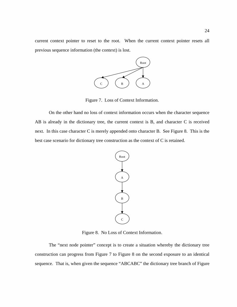
Consider Figure 7 again but with the addition of next node pointers. Next node
pointers represent the sequence ordering in the original string. One next node pointer is from
A to B and another next node pointer is from B to C. The sequence information in the first
exposure of the sequence “ABC” is lost in Figure 7 and is completely intact in Figure 9.
Figure 9. Next Node Pointers for Sequence “ABC”.
From this example it can be seen that the next node pointer reduces the loss of
context information that would normally occur in the standard LZ78 algorithm when the
current context pointer is reset to the root.
4.1.2 Next Node Duplication
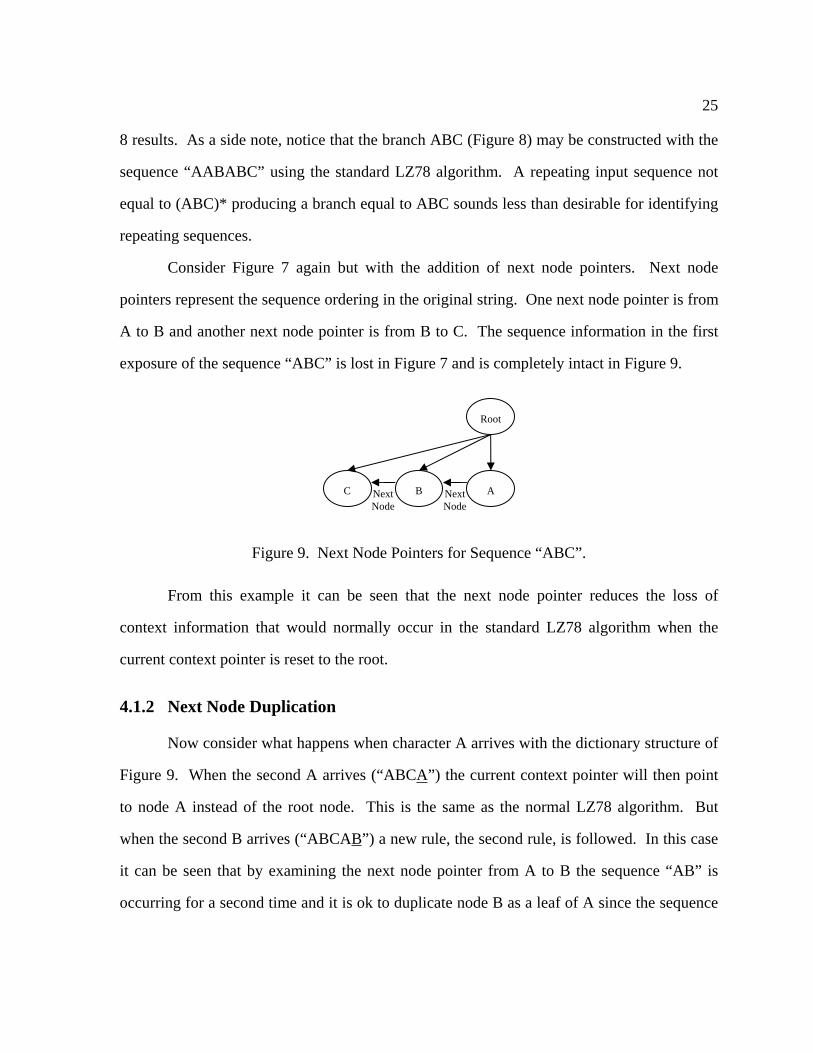
Now consider what happens when character A arrives with the dictionary structure of
Figure 9. When the second A arrives (“ABCA”) the current context pointer will then point
to node A instead of the root node. This is the same as the normal LZ78 algorithm. But
when the second B arrives (“ABCAB”) a new rule, the second rule, is followed. In this case
it can be seen that by examining the next node pointer from A to B the sequence “AB” is
occurring for a second time and it is ok to duplicate node B as a leaf of A since the sequence
Root
ABC Next
Node
Next
Node
26
AB has occurred before. The dictionary tree resulting from the input sequence “ABCAB”,
using next node duplication, is shown in Figure 10.
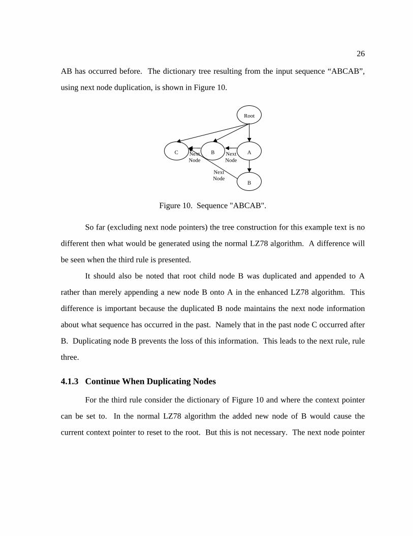
Figure 10. Sequence "ABCAB".
So far (excluding next node pointers) the tree construction for this example text is no
different then what would be generated using the normal LZ78 algorithm. A difference will
be seen when the third rule is presented.
It should also be noted that root child node B was duplicated and appended to A
rather than merely appending a new node B onto A in the enhanced LZ78 algorithm. This
difference is important because the duplicated B node maintains the next node information
about what sequence has occurred in the past. Namely that in the past node C occurred after
B. Duplicating node B prevents the loss of this information. This leads to the next rule, rule
three.
4.1.3 Continue When Duplicating Nodes
For the third rule consider the dictionary of Figure 10 and where the context pointer
can be set to. In the normal LZ78 algorithm the added new node of B would cause the
current context pointer to reset to the root. But this is not necessary. The next node pointer
Root
ABC Next
Node
Next
Node
B
Next
Node
27
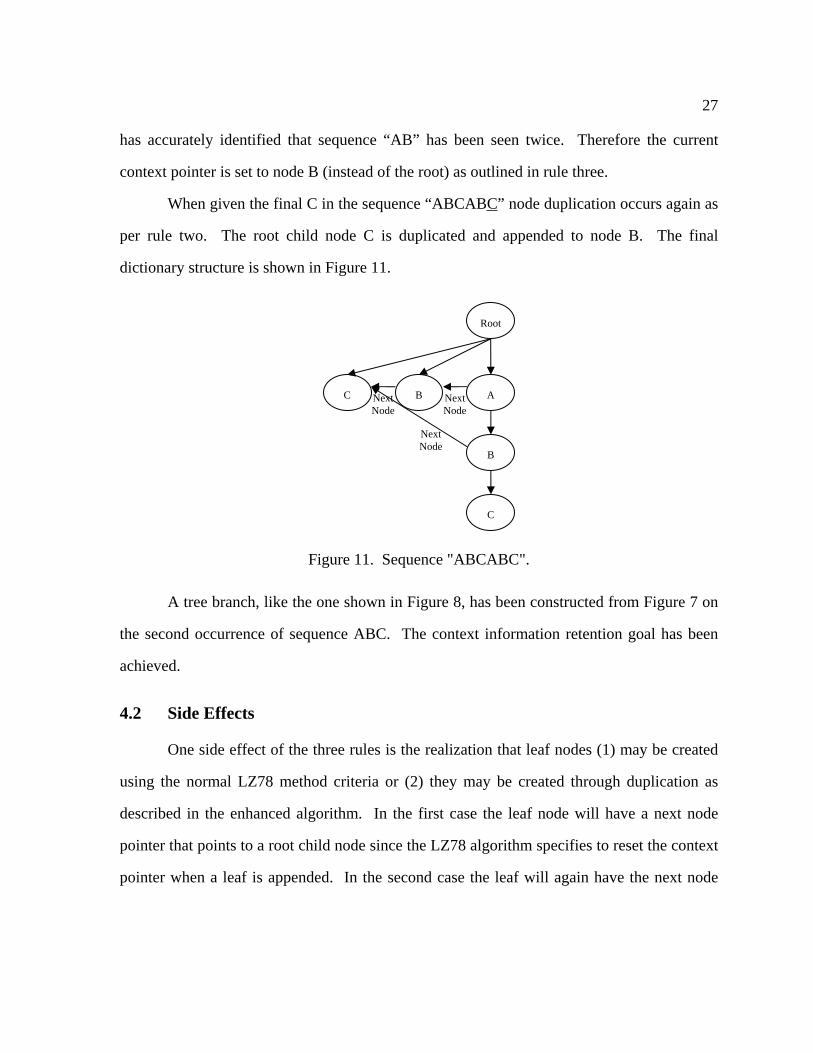
has accurately identified that sequence “AB” has been seen twice. Therefore the current
context pointer is set to node B (instead of the root) as outlined in rule three.
When given the final C in the sequence “ABCABC” node duplication occurs again as
per rule two. The root child node C is duplicated and appended to node B. The final
dictionary structure is shown in Figure 11.
Figure 11. Sequence "ABCABC".
A tree branch, like the one shown in Figure 8, has been constructed from Figure 7 on
the second occurrence of sequence ABC. The context information retention goal has been
achieved.
4.2 Side Effects
One side effect of the three rules is the realization that leaf nodes (1) may be created
using the normal LZ78 method criteria or (2) they may be created through duplication as
described in the enhanced algorithm. In the first case the leaf node will have a next node
pointer that points to a root child node since the LZ78 algorithm specifies to reset the context
pointer when a leaf is appended. In the second case the leaf will again have the next node
Root
ABC Next
Node
Next
Node
B
C
Next
Node

28
pointer that points to a root child node. This is so because the node being duplicated is
always a child of the root and children of the root always have a next node pointer which
points to another child of the root. Children of the root always have next node pointer which
point to another child of the root because when the new root child is created the context
pointer is always reset.
4.3 Learning
Note that in the standard LZ78 dictionary tree construction, one sequence that
constructs Figure 8 (on page 24) would be “AABABC”. With dictionary parsing the
sequence is A, AB, ABC. Another sequence that constructs the branch is
ABC1ABC2ABC3. The sequence parsing is A, B, C, 1, AB, C2, ABC, 3. Note that at least
three exposures are required to construct branch ABC using the standard LZ78 algorithm.
As shown in Figure 11, only two exposures of the sequence ABC were required to construct
the same branch with the enhanced LZ78 algorithm.
From this comparison it can be seen that the enhanced LZ78 algorithm is capable of
learning repeating sequences much faster then the standard LZ78 algorithm. This is
accomplished by speeding the creation of dictionary structures when sequences repeat. It
will always be the case that the first exposure of a sequence of unique symbols will generate
child nodes of the root. It is these child nodes of the root which can be duplicated to create
entire branches when a second repeating sequence occurs in the source.
A best case, or big-Omega, experiment is performed to obtain a lower limit on the
learning rate improvement. The experiment consists of ideal repeating sequence inputs.
Consider, for example, the construction of a dictionary branch ABC using instances of the
sequence ABC. For the standard LZ78 dictionary tree, one sequence (with parsing) which
will construct the branch is:
29
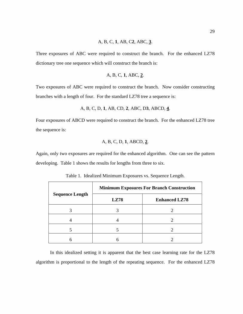
A, B, C, 1, AB, C2, ABC, 3.
Three exposures of ABC were required to construct the branch. For the enhanced LZ78
dictionary tree one sequence which will construct the branch is:
A, B, C, 1, ABC, 2.
Two exposures of ABC were required to construct the branch. Now consider constructing
branches with a length of four. For the standard LZ78 tree a sequence is:
A, B, C, D, 1, AB, CD, 2, ABC, D3, ABCD, 4.
Four exposures of ABCD were required to construct the branch. For the enhanced LZ78 tree
the sequence is:
A, B, C, D, 1, ABCD, 2.
Again, only two exposures are required for the enhanced algorithm. One can see the pattern
developing. Table 1 shows the results for lengths from three to six.
Table 1. Idealized Minimum Exposures vs. Sequence Length.
Minimum Exposures For Branch Construction
Sequence Length
LZ78 Enhanced LZ78
3 3 2
4 4 2
5 5 2
6 6 2
In this idealized setting it is apparent that the best case learning rate for the LZ78
algorithm is proportional to the length of the repeating sequence. For the enhanced LZ78
30
algorithm, the rate is constant. It is possible to learn a sequence in two exposures. In a non
ideal situation, where the next node pointer doesn’t point to the next input symbol, the
enhanced LZ78 learning rate degenerates to the standard LZ78 learning rate.
4.4 Compression and Decompression
The purpose the of the enhanced LZ78 algorithm is to increase the rate of dictionary
tree branch construction. But what are the consequences to the algorithm if the enhancement
was incorporated into a decoder as well? That is, can the enhanced LZ78 encoding algorithm
create code words which could be decoded by an enhanced decoder so that the original text is
compressed and then reconstructed intact? The simplest answer to the question is yes such a
system could be created. The method described here is one of several schemes that may be
possible.
Consider the implementation of the enhancement rules in the decoder and what code
word modifications would be needed to achieve a coding and decoding system. Next node
pointers are easy enough to duplicate in the decoder’s dictionary tree. A next node pointer is
just a pointer assignment between the last two dictionary entries. The fundamental problem
is in the decoder. The decoder must recreate the encoders enhanced dictionary tree in the
decoder’s dictionary tree. To do this it must be able to duplicate nodes as the encoder
duplicates nodes. The decoder must know the difference between (1) adding a dictionary
node via the standard LZ78 way and (2) duplicating one or more nodes via the enhanced
LZ78 way. The following codeword modification is suggested. The modification would
enable the decoder to identify the difference. The format of the proposed codeword is either
of the following depending on the value of flag.
( flag = 0, index, symbol )
( flag = 1, index, length )
31
In the first case, with flag equal to zero, the codeword is exactly the same codeword
as would be used in standard LZ78 coding. This enables nodes to be added to the dictionary
tree in the standard way.
In the second case, with the flag equal to one, the coding would be new. The coding
would be representative of node duplication as described by enhancement rule two. To
explain the new coding, recall the construction of a branch using node duplication. When
duplicating nodes the duplication continues until the node, pointed to by next node pointer,
no longer matches the current node. When the duplication stops the last node on the new
branch is a node created in the standard LZ78 fashion. The new codeword then, is merely a
representation of how many nodes (length) where duplicated on a specific branch (index)
until a standard node is generated. The index and length values on the new codeword take on
those values.
32
CHAPTER 5
ENHANCED LZ78 AND MACRO RECORDING
Given the enhanced sequence learning LZ78 construction described in Chapter 4,
how can the algorithm be used to discover and predict macros? To answer the question lets
first specify formally what a macro is.
Definition: A macro is a sequence of user actions that are repeated.
Implicit in this definition is that there is always some application that receives or is the target
of the user’s actions. Also implied is that a user action may consist of either mouse actions
or a keyboard actions.
Recall from Chapter 3 that the LZ78 algorithm creates a dictionary which can be
viewed as a tree. A macro can be discovered by first quantifying macro like characteristics
and then looking for those characteristics in the tree. From the macro definition above, we
can extrapolate two defining characteristics. A macro has (1) a start point, and (2) an end
point. The job then will be to look for sequences which repeat in the dictionary tree and can
be uniquely identified by pinpointing starting and ending actions.
Intuitively the start point of the macro is the first, or one of the first, symbols in the
dictionary tree and a macro is a sub tree branch. The end point of the macro will require
analysis. A macro in a LZ78 dictionary tree should look something like the structure in
Figure 12.
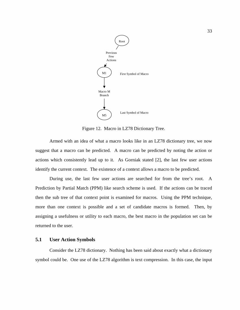
33
Figure 12. Macro in LZ78 Dictionary Tree.
Armed with an idea of what a macro looks like in an LZ78 dictionary tree, we now
suggest that a macro can be predicted. A macro can be predicted by noting the action or
actions which consistently lead up to it. As Gorniak stated [2], the last few user actions
identify the current context. The existence of a context allows a macro to be predicted.
During use, the last few user actions are searched for from the tree’s root. A
Prediction by Partial Match (PPM) like search scheme is used. If the actions can be traced
then the sub tree of that context point is examined for macros. Using the PPM technique,
more than one context is possible and a set of candidate macros is formed. Then, by
assigning a usefulness or utility to each macro, the best macro in the population set can be
returned to the user.
5.1 User Action Symbols
Consider the LZ78 dictionary. Nothing has been said about exactly what a dictionary
symbol could be. One use of the LZ78 algorithm is text compression. In this case, the input
M1
Last Symbol of Macro
Macro M
Branch
M5
Root
Previous
Few
Actions
First Symbol of Macro
34
partition or symbol is an ASCII text character. But the LZ78 algorithm can be used for other
purposes as well. Merely redefining what constitutes a symbol enables us to use the LZ78
algorithm, and more importantly its dictionary, to learn sequences of user actions. For the
algorithm used here, we define a symbol to be a user’s action. Just as ASCII text characters
are symbols in text compression, user actions become the symbols when the LZ78 algorithm
is used to discover and learn macros. The dictionary branches represent learned information
that may be used for imitation.
Having associated LZ78 symbols with user actions the next question becomes what
are the parameters of a user action. A mouse click at a certain screen location is an example.
The action is a mouse click and the screen location is the parameter. The action and its
parameters are used to identify symbol matches. During the dictionary tree construction, a
symbol is considered a match if the symbol has matching parameters. A symbol will not
match if its parameters are different.
Through experiment, the symbols and parameters found necessary to successfully
record and play a sequence of user actions are shown in Table 2. That is to say, most
recorded macros cannot be expected to play properly without at least the parameters
stipulated in the table. It should be noted that the record-play experiment included only a
limited number of desktop applications. Additional symbol parameters would be expected for
a seamless integration of the proposed system into a larger, more encompassing, set of
desktop applications.
35
Table 2. Symbols and their Parameters.
Symbol Parameters
Mouse Button Left / Middle / Right
Down / Up / Down-up
Coordinates
Target Class Name
Target Caption Name
Keyboard Key Virtual Key Code
Down / Up / Down-up
Active Window Change Coordinates
Class Name
Caption Name
In Table 2, a Mouse Button symbol represents a click action of any one of the three
mouse buttons. A “Down-up” symbol occurs when the mouse is not dragged. A separate
“Down” and then “Up” symbol occurs when the mouse is dragged. Additional symbol
parameters include location coordinates X & Y, target window class name, and target window
caption name. The target names are the names of the window which will receive the mouse
click for processing. A Keyboard Key symbol represents a key action on one of the
keyboard keys. Each keyboard key is associated with a Win32 API defined number called
the virtual key code.
An active window change symbol is used to enforce time related consistency between
macro recording and macro playing. When an application is launched some time will occur
before its (parent) window is “active” as defined by Win32 API function call. When an
active window change symbol is encountered in the macro player, playing is suspended until
the current Win32 API defined active window matches the symbol parameter information. In
36
this way, the presence of a new window will be strictly consistent when playing a recorded
macro.
One important aspect with symbol parameters is the characteristics of the sequences
which will be learned. Specifically, with the parameters identified above:
A sequence cannot be learned for a specific document name, independent of
application.
A sequence cannot be learned for a specific application, independent of
document name.
It is possible that three learning systems could be constructed and run simultaneously. One
learning system would use symbols as already described. A second learning system would
employ symbols where application names were not a consideration. Finally a third learning
system would employ symbols where document names were not considered. Macros learned
from all three systems could then be combined into the candidate pool. Such a combined
learning model may have greater use to the user but is not explored here.
Recall from Figure 3 (page 13) that a window is created from the “main thread”. It is
the main thread message pump that receives all keyboard and mouse messages from the
operating system. The thread interprets the messages as it sees fit. This is unlike a UNIX®
X-Window where a mouse and keyboard action maybe associated with a “Widget”. Because
of the interpreting nature of the main thread, an action symbol cannot be directly tied to a
button within a window.
Note that a time stamp symbol, or symbol parameter, has not been defined. This is
because time information is orthogonal to learning a macro sequence. That is, a sequence of
actions may be exhibited to the recording system at any speed. The addition of time stamp
symbols between actions would force all sequences to be twice as long. This would
severally impact the number of exposures required to learn a sequence. In the best case
37
(perfect quantization of time) the learning rate would reduce by a factor of two.
Alternatively, the addition of a time symbol parameter would have a similar detrimental
effect on learning. The user may exhibit a sequence with arbitrary amounts of time between
actions. The learning system is then unable to accurately discern which symbols or actions
match. Regardless, it might be possible to exploit time information to assist in identifying
macro start and end points. The detail of this possibility is not explored here.
5.2 Prediction by Partial Match (PPM)
Prediction by Partial Match (PPM) is a finite context statistical model for text
compression [17]. In this model a symbol is encoded based on an analysis of previously seen
sequences of symbols, or contexts. If the symbol has not been encountered before then no
prediction is made and no special coding takes place. If the symbol has been seen before
then all the sequences leading up to the symbol in the history are enumerated. Usually the
length of prefix sequences is limited to some number such as six. The enumeration forms a
set of tables of prefix strings versus next symbol. One table would be for prefix strings of
length six and another table would be for prefix strings of length five, and so on. These
tables are then used to encode the current symbol in a manor similar to the way a Lempel-Ziv
dictionary table is used. If the current symbol is not found in the prefix length six table then
the prefix length five table is consulted. Analyzing the next lower prefix length is called
“escaping”. Each escape causes an escape codeword to be generated. The index into the
table, of the current symbol to be encoded, becomes the encoder’s outputted codeword.
Arithmetic or Huffman coding is normally used on the index values to further increase
compression.
For example, consider a situation where the current symbol sequence is “…QXYA”
and A is to be encoded. A (hypothetical) search of the symbol history shows that A has
38
occurred only once before. In that case the symbol sequence was “…RXYA”. With a prefix
limit of four, the code words generated would be of the form:
escape, escape, 00 hex.
The encoding algorithm initially searches the prefix length four table. No “A” symbol entry
is found so the first escape codeword is outputted. The prefix length three table is then
searched and once again nothing is found and a second escape is outputted. Finally, the
prefix length two table is searched and A is found and is the only entry. Therefore its index
value is 0 hex. The index value of 0 hex is then outputted.
The Prediction by Partial Match technique is used here to identify macro contexts.
Just as text characters are used as symbols in the PPM algorithm, PC user actions are the
symbols used to learn macros. Consider the case where the two user actions “XY” can
predict the next symbol. In the PPM scheme, the prefix length two table is consulted. If XY
is an entry (there is a history of XY in the past) then the table entry predicts the next symbol.
Now consider an analogous situation in an LZ78 dictionary tree. The root of the tree is
scanned for X followed by Y. If the XY trace does not exist in the tree then no macro is
predicted. If XY does exist then the sub tree, rooted at Y, is searched for macros. All
macros found at Y are then put into a pool. In the terminology used in this thesis, any
qualifying macro is placed into the “candidate pool” or “candidate population”.
Consider the case where the last few actions are not just XY but is actually WXY. If
WXY can be traced from the root of the dictionary tree, then the macros found in that sub
tree are also added to the candidate population. In fact all the short prefix lengths are
scanned for in the dictionary tree. All macros found are added to the candidate population.

39
If context search computational overhead is not a concern longer prefix lengths can
be considered and added to the candidate population. Specifically if the depth of the LZ78
dictionary tree is managed, context prefix lengths up to the tree depth can be considered.
5.3 Macro Start Point
Even though the goal of identifying a macro is finding repeating actions, it must be
realized that repeating sequences have preceding actions. Presumably, the preceding or
prefixing actions may be classified as either (1) related to the macro or (2) unrelated to the
macro. Related prefixing symbols may be said to provide context information. Unrelated
prefixing symbols are random in nature and provide no hint or evidence as to what the next
symbol, or macro, might be.
In the first case, with related prefixing symbols, the LZ78 algorithm is beneficial as
macro sequences are built as sub trees to prefix symbols. The prefixing symbols can then be
used as predictors of upcoming macro sequences as discussed in the PPM section. The
prefixing symbols become the macro’s context. Symbols before the prefix symbols are
normally unrelated which causes the prefix symbols to be children of the root.
As discussed in Chapter 3, the enhanced LZ78 algorithm can build a sub tree branch
in as few as two sequence exposures. In a similar manor, the two (prefix symbol) branches
shown in Figure 13 can be built in as few as three sequence exposures.
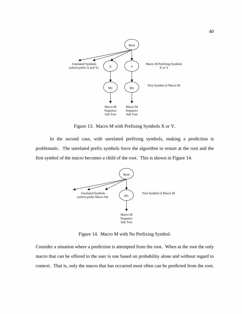
40
Figure 13. Macro M with Prefixing Symbols X or Y.
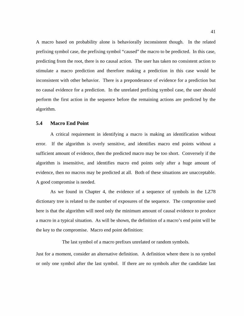
In the second case, with unrelated prefixing symbols, making a prediction is
problematic. The unrelated prefix symbols force the algorithm to restart at the root and the
first symbol of the macro becomes a child of the root. This is shown in Figure 14.
Figure 14. Macro M with No Prefixing Symbol.
Consider a situation where a prediction is attempted from the root. When at the root the only
macro that can be offered to the user is one based on probability alone and without regard to
context. That is, only the macro that has occurred most often can be predicted from the root.
Unrelated Symbols
(which prefix Macro M)
Root
M1 First Symbol of Macro M
Macro M
Sequence
Sub Tree
Macro M Prefixing Symbols
X or Y
Unrelated Symbols
(which prefix X and Y)
Root
Y
Macro M
Sequence
Sub Tree
X
Macro M
Sequence
Sub Tree
M1 M1 First Symbol of Macro M
41
A macro based on probability alone is behaviorally inconsistent though. In the related
prefixing symbol case, the prefixing symbol “caused” the macro to be predicted. In this case,
predicting from the root, there is no causal action. The user has taken no consistent action to
stimulate a macro prediction and therefore making a prediction in this case would be
inconsistent with other behavior. There is a preponderance of evidence for a prediction but
no causal evidence for a prediction. In the unrelated prefixing symbol case, the user should
perform the first action in the sequence before the remaining actions are predicted by the
algorithm.
5.4 Macro End Point
A critical requirement in identifying a macro is making an identification without
error. If the algorithm is overly sensitive, and identifies macro end points without a
sufficient amount of evidence, then the predicted macro may be too short. Conversely if the
algorithm is insensitive, and identifies macro end points only after a huge amount of
evidence, then no macros may be predicted at all. Both of these situations are unacceptable.
A good compromise is needed.
As we found in Chapter 4, the evidence of a sequence of symbols in the LZ78
dictionary tree is related to the number of exposures of the sequence. The compromise used
here is that the algorithm will need only the minimum amount of causal evidence to produce
a macro in a typical situation. As will be shown, the definition of a macro’s end point will be
the key to the compromise. Macro end point definition:
The last symbol of a macro prefixes unrelated or random symbols.
Just for a moment, consider an alternative definition. A definition where there is no symbol
or only one symbol after the last symbol. If there are no symbols after the candidate last
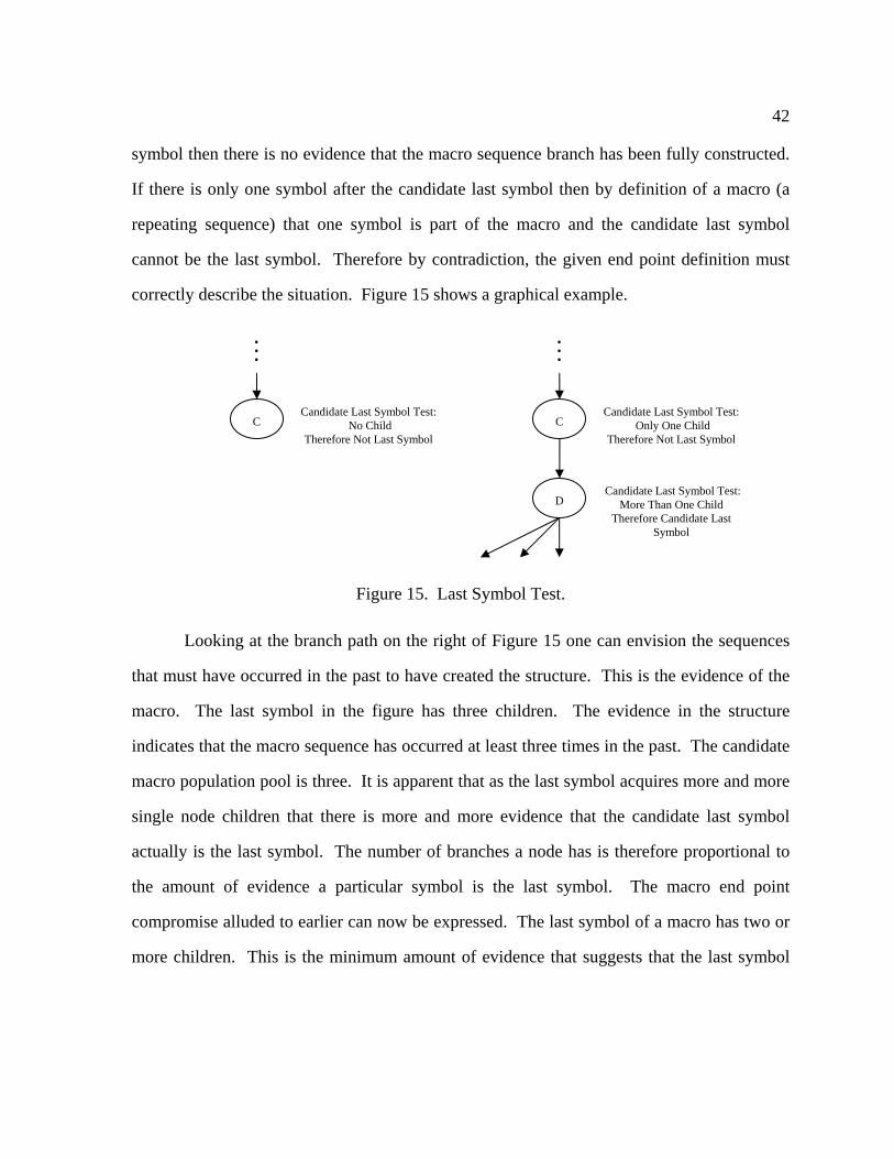
42
symbol then there is no evidence that the macro sequence branch has been fully constructed.
If there is only one symbol after the candidate last symbol then by definition of a macro (a
repeating sequence) that one symbol is part of the macro and the candidate last symbol
cannot be the last symbol. Therefore by contradiction, the given end point definition must
correctly describe the situation. Figure 15 shows a graphical example.
Figure 15. Last Symbol Test.
Looking at the branch path on the right of Figure 15 one can envision the sequences
that must have occurred in the past to have created the structure. This is the evidence of the
macro. The last symbol in the figure has three children. The evidence in the structure
indicates that the macro sequence has occurred at least three times in the past. The candidate
macro population pool is three. It is apparent that as the last symbol acquires more and more
single node children that there is more and more evidence that the candidate last symbol
actually is the last symbol. The number of branches a node has is therefore proportional to
the amount of evidence a particular symbol is the last symbol. The macro end point
compromise alluded to earlier can now be expressed. The last symbol of a macro has two or
more children. This is the minimum amount of evidence that suggests that the last symbol
Candidate Last Symbol Test:
More Than One Child
Therefore Candidate Last
Symbol
Candidate Last Symbol Test:
Only One Child
Therefore Not Last Symbol
. . .
C
D
Candidate Last Symbol Test:
No Child
Therefore Not Last Symbol
. . .
C
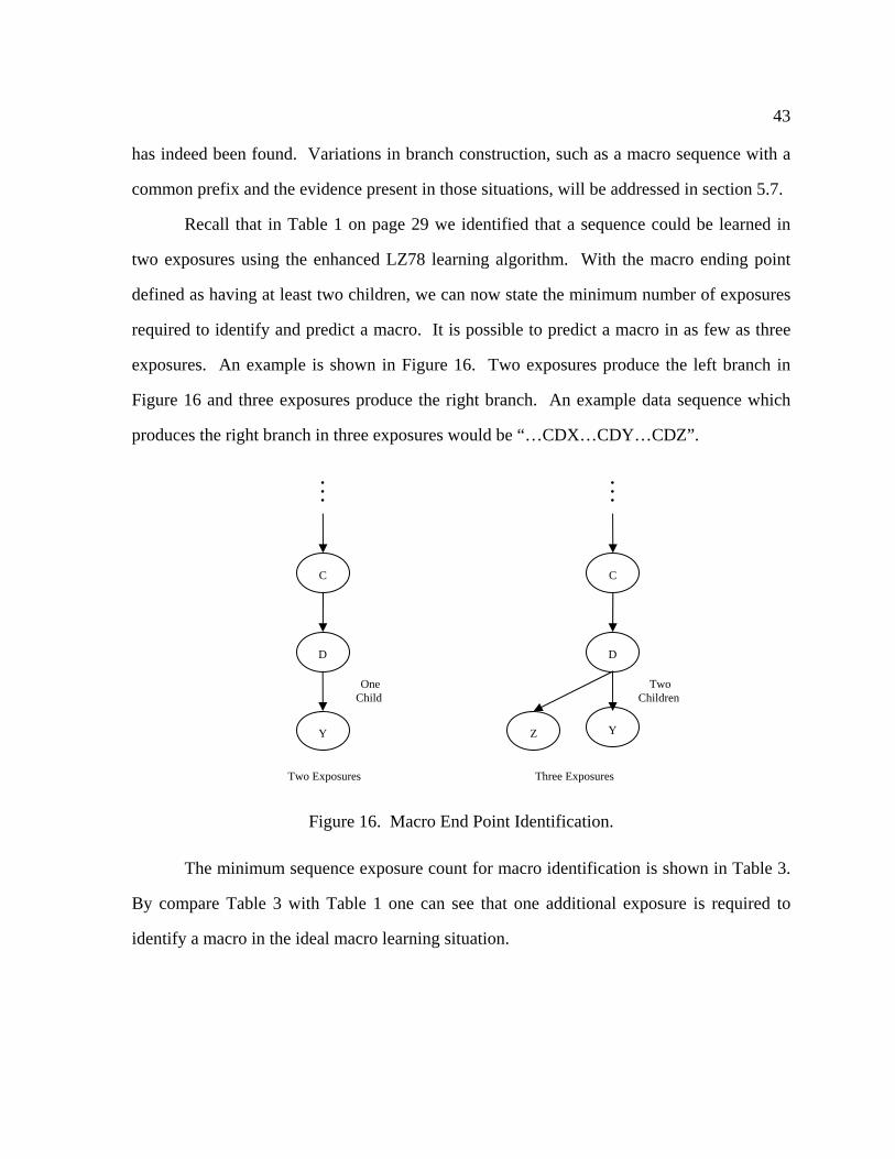
43
has indeed been found. Variations in branch construction, such as a macro sequence with a
common prefix and the evidence present in those situations, will be addressed in section 5.7.
Recall that in Table 1 on page 29 we identified that a sequence could be learned in
two exposures using the enhanced LZ78 learning algorithm. With the macro ending point
defined as having at least two children, we can now state the minimum number of exposures
required to identify and predict a macro. It is possible to predict a macro in as few as three
exposures. An example is shown in Figure 16. Two exposures produce the left branch in
Figure 16 and three exposures produce the right branch. An example data sequence which
produces the right branch in three exposures would be “…CDX…CDY…CDZ”.
Figure 16. Macro End Point Identification.
The minimum sequence exposure count for macro identification is shown in Table 3.
By compare Table 3 with Table 1 one can see that one additional exposure is required to
identify a macro in the ideal macro learning situation.
Two
Children
C
D
Y
Two Exposures
. . .
C
D
Y
. . .
Z
Three Exposures
One
Child

44
Table 3. Idealized Minimum Exposures vs. Macro Length.
Minimum Exposures For Macro Identification Macro Length
LZ78 Enhanced LZ78
3 4 3
4 5 3
5 6 3
6 7 3
5.5 Symbol vs. Sequence Probabilities
An important understanding in evaluating the dictionary tree for macros is realizing
that sequences can be counted as well as symbols. This is important from a probability
calculation stand point. For example consider the tree structure shown in Figure 17. The
symbol visitation counts are given to the right of each symbol.
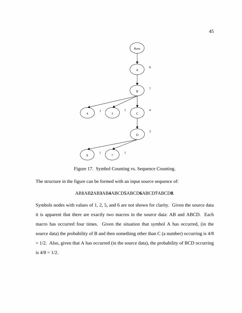
45
Figure 17. Symbol Counting vs. Sequence Counting.
The structure in the figure can be formed with an input source sequence of:
AB1AB2AB3AB4ABCD5ABCD6ABCD7ABCD8.
Symbols nodes with values of 1, 2, 5, and 6 are not shown for clarity. Given the source data
it is apparent that there are exactly two macros in the source data: AB and ABCD. Each
macro has occurred four times. Given the situation that symbol A has occurred, (in the
source data) the probability of B and then something other than C (a number) occurring is 4/8
= 1/2. Also, given that A has occurred (in the source data), the probability of BCD occurring
is 4/8 = 1/2.
3
8
7
4 1
1 1
Root
A
B
3 C
7
D
1 4
8
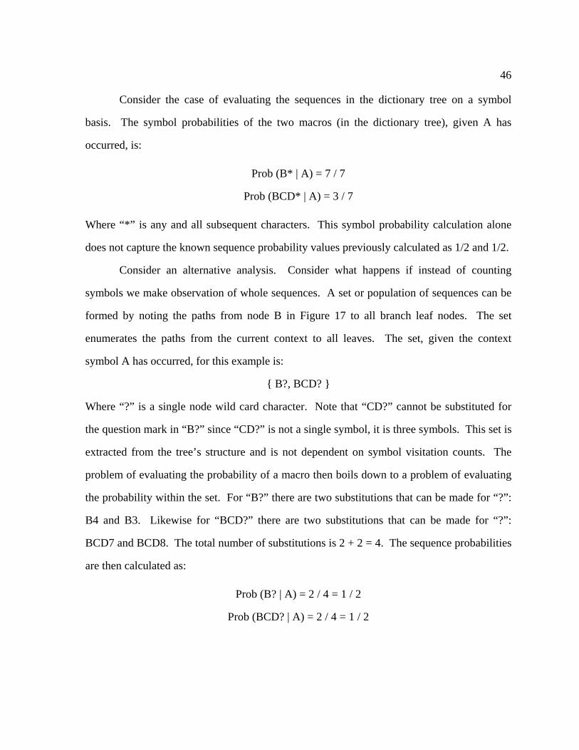
46
Consider the case of evaluating the sequences in the dictionary tree on a symbol
basis. The symbol probabilities of the two macros (in the dictionary tree), given A has
occurred, is:
Prob (B* | A) = 7 / 7
Prob (BCD* | A) = 3 / 7
Where “*” is any and all subsequent characters. This symbol probability calculation alone
does not capture the known sequence probability values previously calculated as 1/2 and 1/2.
Consider an alternative analysis. Consider what happens if instead of counting
symbols we make observation of whole sequences. A set or population of sequences can be
formed by noting the paths from node B in Figure 17 to all branch leaf nodes. The set
enumerates the paths from the current context to all leaves. The set, given the context
symbol A has occurred, for this example is:
{ B?, BCD? }
Where “?” is a single node wild card character. Note that “CD?” cannot be substituted for
the question mark in “B?” since “CD?” is not a single symbol, it is three symbols. This set is
extracted from the tree’s structure and is not dependent on symbol visitation counts. The
problem of evaluating the probability of a macro then boils down to a problem of evaluating
the probability within the set. For “B?” there are two substitutions that can be made for “?”:
B4 and B3. Likewise for “BCD?” there are two substitutions that can be made for “?”:
BCD7 and BCD8. The total number of substitutions is 2 + 2 = 4. The sequence probabilities
are then calculated as:
Prob (B? | A) = 2 / 4 = 1 / 2
Prob (BCD? | A) = 2 / 4 = 1 / 2

47
This sequence probability calculation appears to be more accurate than the symbol
probability calculation. The sequence probability calculation here matches the sequence
probability calculation on the source data. They are both 1/2.
The probability of macro Mi may be calculated on a per-symbol or a per-sequence
basis as either:
Prob (Mi * | Context) symbol probability
Prob (Mi ? | Context) sequence probability
Regardless of which probability metric is used or is preferred, the generic probability
term that will be used in subsequent sections is: Prob(Mi).
5.6 Macro Utility
Each macro can be characterized by its worth or utility to the user. In a macro
learning environment there are two components in evaluating utility. One component, the
benefit component, is the weight of predicting a macro correctly. The other component, the
cost component, is the weight of predicting a macro incorrectly. If the prediction is correct
then the utility should increase and if the prediction is incorrect then the utility should
decrease. The ability to make a prediction of a macro is based on the probability that the
macro will occur. The probability that it will occur is Prob(Mi) and the probability that it
will not occur is (1 - Prob(Mi)).
In some situations it may be more desirable to give additional credence to longer
macros since longer macros reduce the total amount of user work. The benefit should
linearly increase with the length of the macro. The amount of benefit and cost for a given
macro (Mi) are thus given by:

48
Benefit (Mi) = Prob (Mi) * Length of Mi * Benefit Constant
Cost (Mi) = (1 - Prob (Mi)) * Cost Constant.
The Benefit Constant and the Cost Constant are relative terms used to balance the two
components. If the costs are relatively equal then the constants may be evaluated to one.
Finally, the utility (Utilityi) of each macro (Mi) is given by:
Utilityi (Mi) = Benefit (Mi) - Cost (Mi) – Utility Constant
The Utility Constant represents the amount of obtrusiveness the program has on the user to
invoke the macro of choice. For experimental purposes a value of zero may be suitable.
Once each macro is assigned a utility, the population of candidate macros can be
ranked. In this way the macro with the highest utility ranking can be forwarded to the user.
In addition, a minimum utility threshold value may be set. With this criterion, the utility of a
macro must exceed a certain threshold value before the macro is allowed to be returned to the
user. More than one macro may be forwarded to the user in this case. Alternately, a
fractional set of high ranking macros from the candidate population may be returned to the
user. To extract this set a utility cut-off value representative of the fraction is determined.
This value then becomes the threshold utility value. The utility of each candidate macro is
compared to the cut-off threshold value. Only macros with utilities higher than the cut-off
threshold are returned to the user.
5.7 Example Situations
Some macro sequence permutations produce distinctive dictionary tree structures.
Several representative dictionary tree structures, and the calculation of their sequence
probability, are presented in this section.
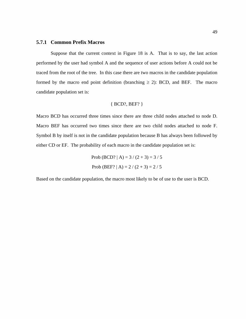
49
5.7.1 Common Prefix Macros
Suppose that the current context in Figure 18 is A. That is to say, the last action
performed by the user had symbol A and the sequence of user actions before A could not be
traced from the root of the tree. In this case there are two macros in the candidate population
formed by the macro end point definition (branching 2): BCD, and BEF. The macro
candidate population set is:
{ BCD?, BEF? }
Macro BCD has occurred three times since there are three child nodes attached to node D.
Macro BEF has occurred two times since there are two child nodes attached to node F.
Symbol B by itself is not in the candidate population because B has always been followed by
either CD or EF. The probability of each macro in the candidate population set is:
Prob (BCD? | A) = 3 / (2 + 3) = 3 / 5
Prob (BEF? | A) = 2 / (2 + 3) = 2 / 5
Based on the candidate population, the macro most likely to be of use to the user is BCD.
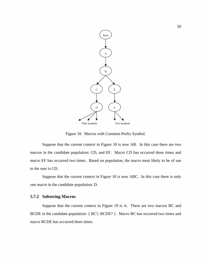
50
Figure 18. Macros with Common Prefix Symbol.
Suppose that the current context in Figure 18 is now AB. In this case there are two
macros in the candidate population: CD, and EF. Macro CD has occurred three times and
macro EF has occurred two times. Based on population, the macro most likely to be of use
to the user is CD.
Suppose that the current context in Figure 18 is now ABC. In this case there is only
one macro in the candidate population: D.
5.7.2 Substring Macros
Suppose that the current context in Figure 19 is A. There are two macros BC and
BCDE in the candidate population: { BC?, BCDE? }. Macro BC has occurred two times and
macro BCDE has occurred three times.
Root
A
B
C E
D F
Thee Symbols Two Symbols
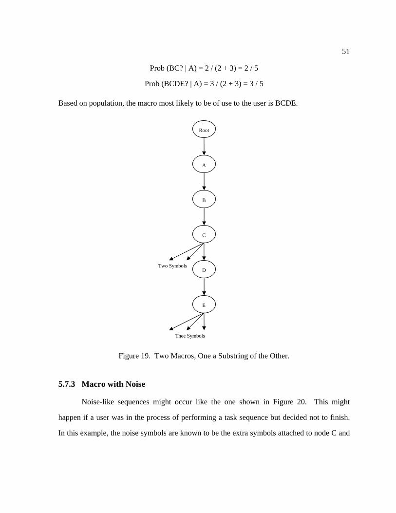
51
Prob (BC? | A) = 2 / (2 + 3) = 2 / 5
Prob (BCDE? | A) = 3 / (2 + 3) = 3 / 5
Based on population, the macro most likely to be of use to the user is BCDE.
Figure 19. Two Macros, One a Substring of the Other.
5.7.3 Macro with Noise
Noise-like sequences might occur like the one shown in Figure 20. This might
happen if a user was in the process of performing a task sequence but decided not to finish.
In this example, the noise symbols are known to be the extra symbols attached to node C and
Root
A
B
C
E
D
Thee Symbols
Two Symbols
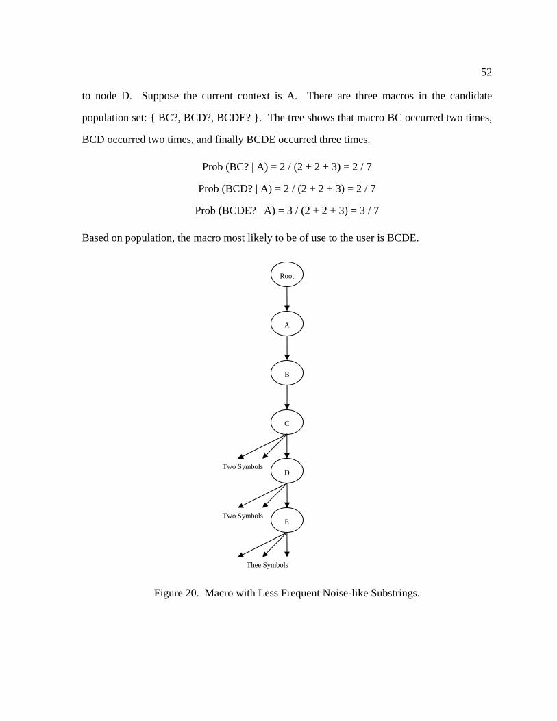
52
to node D. Suppose the current context is A. There are three macros in the candidate
population set: { BC?, BCD?, BCDE? }. The tree shows that macro BC occurred two times,
BCD occurred two times, and finally BCDE occurred three times.
Prob (BC? | A) = 2 / (2 + 2 + 3) = 2 / 7
Prob (BCD? | A) = 2 / (2 + 2 + 3) = 2 / 7
Prob (BCDE? | A) = 3 / (2 + 2 + 3) = 3 / 7
Based on population, the macro most likely to be of use to the user is BCDE.
Figure 20. Macro with Less Frequent Noise-like Substrings.
Root
A
B
C
E
D
Thee Symbols
Two Symbols
Two Symbols
53
CHAPTER 6
PERFORMANCE STUDY
When making drastic changes to an algorithm, side effect questions naturally surface.
What is the effect on the number of nodes in the dictionary tree? Is the compression ratio
now higher? To address these questions the LZ78 and the enhanced LZ78 encoding
algorithms were implemented and fed with identical input data. With identical input, the
approximate amount of compression and the number of dictionary nodes can be directly
compared. A variety of input files where evaluated. In general, it was found that the amount
of compression afforded by the algorithm depended on the type or format of input data.
Notable improvements in compression performance were noted with “.BMP”, and to a lesser
extent “.XLS”, file formats with the enhanced LZ78 algorithm. Also, the increased
compression performance normally coincided with a large number of nodes in the enhanced
LZ78 dictionary tree. Compression performance of other file formats, in general, depended
on the specific file at hand. With some files the LZ78 algorithm exhibited slightly better
compression and with other files the enhanced LZ78 algorithm exhibited slightly better
compression performance. From these tests one would expect that in cases where file
compression performance improved that duplication of long chains of nodes had occurred.
In the context of this thesis, these duplicated node chains are macros.
6.1 Representative Scenario
Further tests were conducted with realistic scenarios in mind to gain additional
insight. A “printing” macro test scenario was created in a situational environment likely to
occur. The goal of the test was to gather statistics so that the learning rate of the standard
54
LZ78 algorithm could be directly compared with the learning rate of the enhanced LZ78
algorithm.
The test scenario calls for the user to launch a file from a desktop shortcut and then
print the file with a certain consistent set of options. The user closes the file and then works
in other applications. The user repeats this process many times. The idea of the scenario is
that the printed document is, for example, a report that must be printed for a weekly team
meeting. The user works in other applications during the week and only at specific times
does the document need to be printed and when doing so it needs to be printed in its own
special way.
The job of the macro learning algorithm is to learn the consistent actions of the user.
In this example the actions are printing a certain document in a certain way. Other user
actions occur before and after the macro of interest. The sequence to be learned is shown in
Table 4.
The macro sequence of interest is then embedded within other symbols. The other
symbols represent other user actions in other applications. For the macro learning system to
succeed, the sequence of interest must be discovered and learned while other user activity is
occurring. The entire desktop simulation sequence with embedded macro subsequence is
shown in Table 5. Items identified with “*” are random numbers with the range specified. A
new random number is generated each iteration.
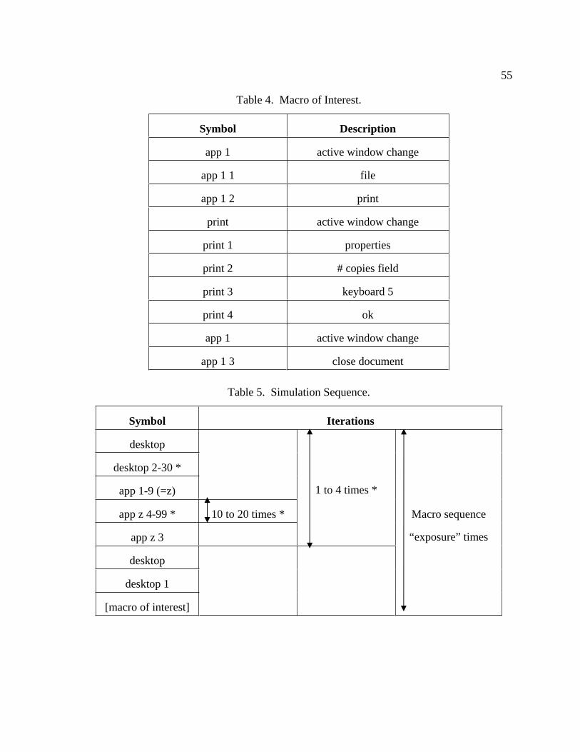
55
Table 4. Macro of Interest.
Symbol Description
app 1 active window change
app 1 1 file
app 1 2 print
print active window change
print 1 properties
print 2 # copies field
print 3 keyboard 5
print 4 ok
app 1 active window change
app 1 3 close document
Table 5. Simulation Sequence.
Symbol Iterations
desktop
desktop 2-30 *
app 1-9 (=z)
app z 4-99 * 10 to 20 times *
app z 3
1 to 4 times *
desktop
desktop 1
[macro of interest]
Macro sequence
“exposure” times
56
In this simulation the macro of interest has two prefixing symbols: “desktop” and
“desktop 1”. As one can see from the symbol column, symbol “desktop” prefixes other
actions in other application sequences. Note the “z” on rows three, four and five. Symbol
“z” takes on the value of one through nine in line three and the value is transferred to lines
four and five. In essence, the macro sequence of interest is intermixed with eight other
applications.
The sequence in Table 5 is repeated 400 times (400 trials) and error statistics were
colleted and averaged. The results are shown in Table 6 and Table 7. Table 6 contains the
results for the standard LZ78 algorithm and Table 7 contains the results for the enhanced
LZ78 algorithm. The macro extraction and prediction algorithm is the same for both
dictionary construction methods.
If the extraction algorithm made an average of zero predictions in the 400 trials then a
value of 0 is entered in the “none” row. If the algorithm predicted one or more macros then
their utility was measured. The macro with the highest utility is the algorithm’s prediction.
The macro benefit constant and macro cost constant relational variables were statically set to
one since the goal of the experiment is to compare learning rates. The macro predicted by
the algorithm was then compared with the macro of interest. Any errors in symbols were
recorded and averaged over the number of trials.
If the algorithm made a prediction but the returned sequence was either too long or
too short in length then the rows labeled “tooShort” or “tooLong” are filled in. If the
algorithm made a prediction, and the length was ok, but one or more mnemonic symbols
were incorrect then the “mismatch” row is filled in. If the algorithm made a prediction and
the prediction was 100% correct then the row labeled “correct” is filled in. The average
number of LZ78 dictionary nodes is shown in the “Number Nodes” row. Finally if the
algorithm were to be used to output compressed code words then the approximate amount of
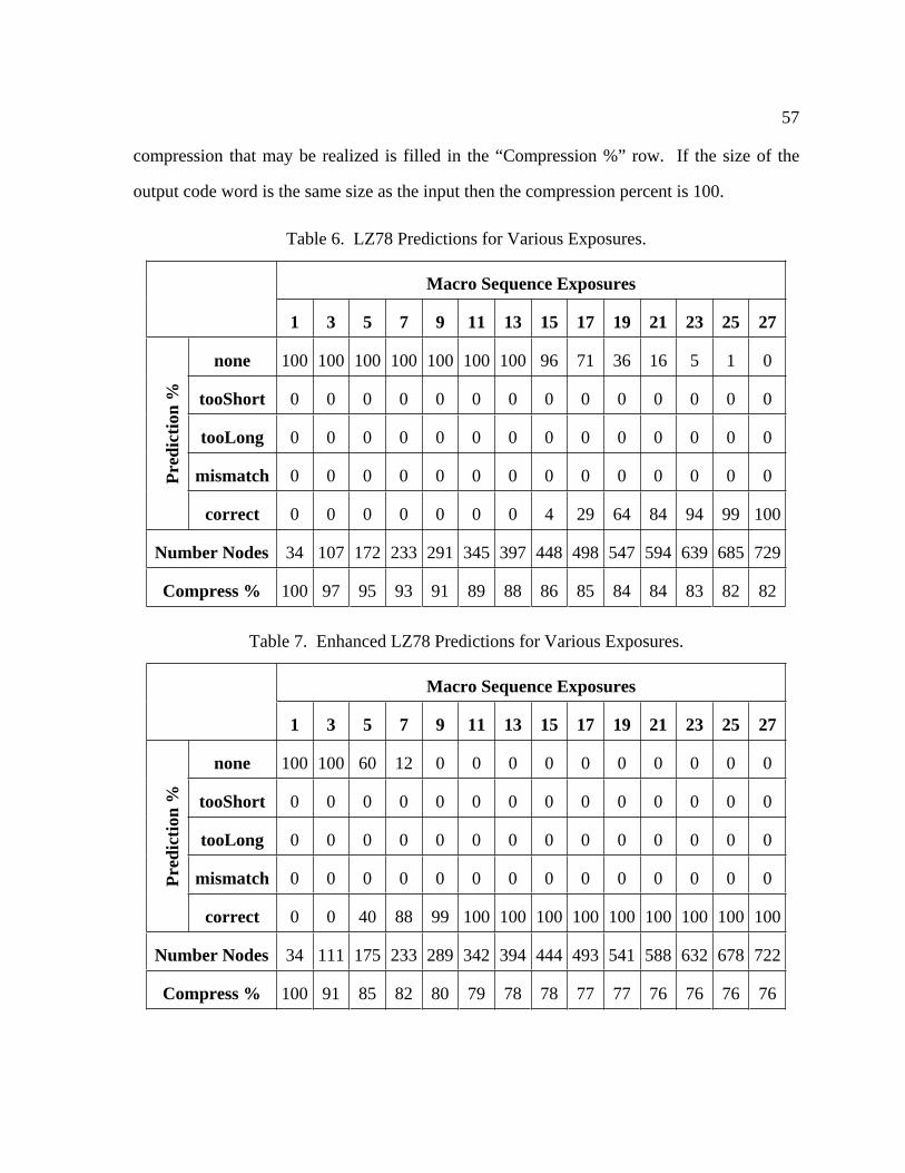
57
compression that may be realized is filled in the “Compression %” row. If the size of the
output code word is the same size as the input then the compression percent is 100.
Table 6. LZ78 Predictions for Various Exposures.
Macro Sequence Exposures
1 3 5 7 9 11 13 15 17 19 21 23 25 27
none 100 100 100 100 100 100 100 96 71 36 16 5 1 0
tooShort 0 0 0 0 0 0 0 0 0 0 0 0 0 0
tooLong 0 0 0 0 0 0 0 0 0 0 0 0 0 0
mismatch 0 0 0 0 0 0 0 0 0 0 0 0 0 0 Pre
dic
tio
n %
correct 0 0 0 0 0 0 0 4 29 64 84 94 99 100
Number Nodes 34 107 172 233 291 345 397 448 498 547 594 639 685 729
Compress % 100 97 95 93 91 89 88 86 85 84 84 83 82 82
Table 7. Enhanced LZ78 Predictions for Various Exposures.
Macro Sequence Exposures
1 3 5 7 9 11 13 15 17 19 21 23 25 27
none 100 100 60 12 0 0 0 0 0 0 0 0 0 0
tooShort 0 0 0 0 0 0 0 0 0 0 0 0 0 0
tooLong 0 0 0 0 0 0 0 0 0 0 0 0 0 0
mismatch 0 0 0 0 0 0 0 0 0 0 0 0 0 0 Pre
dic
tio
n %
correct 0 0 40 88 99 100 100 100 100 100 100 100 100 100
Number Nodes 34 111 175 233 289 342 394 444 493 541 588 632 678 722
Compress % 100 91 85 82 80 79 78 78 77 77 76 76 76 76
58
By comparing the “correct” rows in Table 6 and Table 7 it can be seen that the
learning rates are different between the algorithms. The macro of interest in this experiment
has a length of ten symbols and a context prefix length of two symbols. The macro was
learned with 100% effectiveness in 11 exposures using the enhanced LZ78 algorithm and in
27 exposures using the normal LZ78 algorithm. The learning rate in this example has
improved by a factor of about 2.5.
6.1.1 Number of Tree Nodes
One point worth mentioning about Table 6 and Table 7 is the number of nodes in the
dictionary trees. The number of nodes in the enhanced LZ78 tree is slightly less than the
number of nodes in the standard LZ78 tree after seven exposures. To explain this
phenomenon, consider the converged structural differences between the algorithms. Figure
21 is a generalization of a dictionary tree structure containing the four symbol macro ABCD.
Unrelated symbols in the alphabet are not shown in the generalization. Also not shown are
node symbols A, B, C, and D that may be appended to those unrelated symbols.
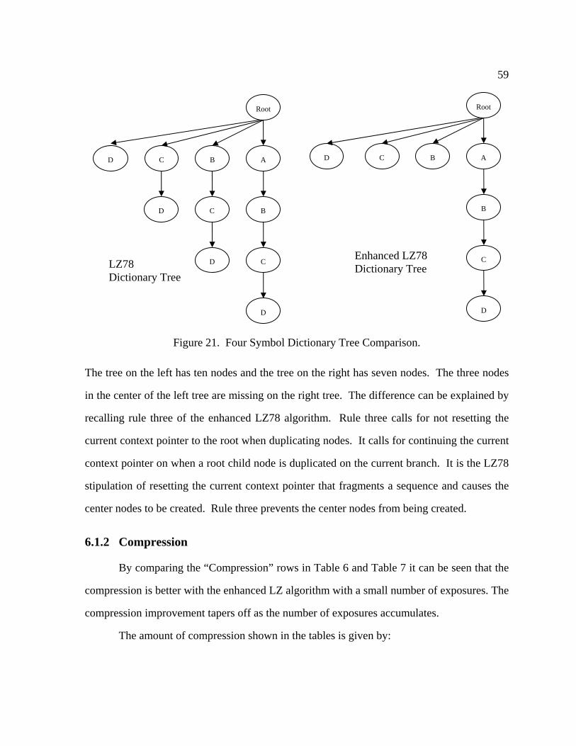
59
Figure 21. Four Symbol Dictionary Tree Comparison.
The tree on the left has ten nodes and the tree on the right has seven nodes. The three nodes
in the center of the left tree are missing on the right tree. The difference can be explained by
recalling rule three of the enhanced LZ78 algorithm. Rule three calls for not resetting the
current context pointer to the root when duplicating nodes. It calls for continuing the current
context pointer on when a root child node is duplicated on the current branch. It is the LZ78
stipulation of resetting the current context pointer that fragments a sequence and causes the
center nodes to be created. Rule three prevents the center nodes from being created.
6.1.2 Compression
By comparing the “Compression” rows in Table 6 and Table 7 it can be seen that the
compression is better with the enhanced LZ algorithm with a small number of exposures. The
compression improvement tapers off as the number of exposures accumulates.
The amount of compression shown in the tables is given by:
Root
ABCD
B
C
D
C
D
D
Root
A
B
C
D
BCD
LZ78
Dictionary Tree
Enhanced LZ78
Dictionary Tree
60
Number of Codeword Symbols * Bits per Codeword Compression Percent = * 100.
Number of Input Symbols * Bits per Input Symbol
If the number of code word symbols equals the number of input symbols then no
compression has taken place and the compression percent is 100. In this calculation, the
ratio of bits per codeword to bits per input symbol is approximated. The approximation has
two components. One approximation is that the number of bits in a “(null, non matching
character)” codeword is the same number of bits as the number of bits in an input symbol.
With this approximation the compression ratio is 100 percent, as defined above, and occurs
as children of the root are added to the dictionary tree. The other approximation component
is that the number of bits in a “(dictionary index, non matching character)” codeword is twice
the number of bits as a “(null, non matching character)” codeword. This is the typical
converging case as the dictionary fills to capacity with entries. In reality, the number of bits
in an input symbol and the number of bits in a codeword are implementation dependent and
their ratio varies as the dictionary tree grows.
A graph of the approximate amount of compression from one to 27 exposures for this
example scenario is shown in Figure 22. In the figure we can see that compression
performance of the enhanced LZ78 algorithm improves quickly as compared to the standard
LZ78 algorithm (LZ). A graph of the approximate amount of compression from one to 500
exposures is shown in Figure 23. In the figure we can more clearly see that the amount of
compression for the two different algorithms is converging very slowly.
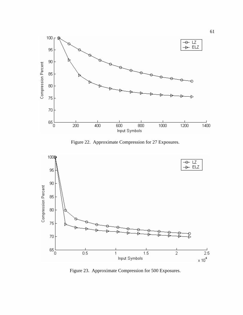
61
Figure 22. Approximate Compression for 27 Exposures.
Figure 23. Approximate Compression for 500 Exposures.
62
It should be noted that most Lempel-Ziv compression schemes in use today also
employ arithmetic coding on top of Lempel-Ziv coding to further improve the compression
ratio [17].
6.1.3 Macro Subsuming
Recall from section 5.5 that a macro’s probability may be calculated based on either
symbol probability or sequence probability. Also recall the Benefit(Mi) calculation on page
47. In that calculation the symbol probability was multiplied by the sequence’s length in
order to not put undo preference to shorter sequences.
Consider another case, a case where the desired macro has occurred hundreds of
times. In this case the dictionary tree structure, and the branch of the macro of interest, is
rich with leaves and branches. Given a bounded symbol alphabet, eventually the desired
macro is subsumed by longer sequences. The leaves, attached to the end of the branch of the
macro of interest, turn into branches. To analyze the effect, experiments were made using
the simulation sequence of Table 5 but with many more exposures. The effects of symbol
probability and sequence probability were also included. The results are shown in Table 8.
As we saw in Table 6 and Table 7, the minimum number of macro exposures required for
100% correct subsequent predictions is 27 exposures with the LZ78 algorithm and 11
exposures for the enhanced LZ78 algorithm. Here we see in Table 8 that, after a large
number of exposures, the algorithm fails to predict the macro of interest with certainty. This
is shown in the last row. After the number of exposures specified, the algorithm begins to
predict macros that are longer than the macro of interest instead of the macro of interest. The
macro of interest becomes subsumed.

63
Table 8. Over Exposure Effects.
Dictionary Type & Probability Method
LZ Enhanced LZ
Sym Seq Sym Seq
Minimum number of macro exposures for 100% correct predictions
27 27 11 11
Maximum number of macro exposures for 100% correct predictions
379 253 379 211
One can see from the table that in the enhanced LZ78 dictionary tree, symbol
counting fairs better than sequence counting after 211 exposures. That is to say, a macro
longer than the one defined in the experiment may be given to the user after 211 exposures of
the desired macro. This improved symbol probability effect can be understood by realizing
that shorter length macros, which have symbols that have occurred in a preponderance of the
times, will be given greater utility as the number of exposures increases. On the other hand,
the sequence probability will dwindle towards zero as leaves attached to the macro become
branches.
6.2 Noise Substring Scenario
A more difficult macro extraction scenario experiment, with common symbol
substrings, was performed. The scenario is similar to the one shown in Figure 20 on page 52.
The simulation sequence for the macro of interest is unchanged for this experiment but the
desired macro is intermixed with substrings macros of the desired macro. There are four
substrings macros and are shown as columns A, B, C, and D in Table 9. The “print 5”
mnemonic in the noise sequences represents closing the print window prematurely.
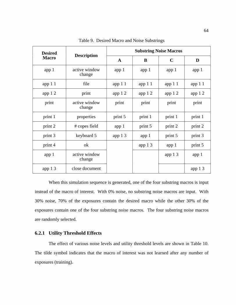
64
Table 9. Desired Macro and Noise Substrings
Substring Noise Macros DesiredMacro
DescriptionA B C D
app 1 active window change
app 1 app 1 app 1 app 1
app 1 1 file app 1 1 app 1 1 app 1 1 app 1 1
app 1 2 print app 1 2 app 1 2 app 1 2 app 1 2
print active window change
print print print print
print 1 properties print 5 print 1 print 1 print 1
print 2 # copes field app 1 print 5 print 2 print 2
print 3 keyboard 5 app 1 3 app 1 print 5 print 3
print 4 ok app 1 3 app 1 print 5
app 1 active window change
app 1 3 app 1
app 1 3 close document app 1 3
When this simulation sequence is generated, one of the four substring macros is input
instead of the macro of interest. With 0% noise, no substring noise macros are input. With
30% noise, 70% of the exposures contain the desired macro while the other 30% of the
exposures contain one of the four substring noise macros. The four substring noise macros
are randomly selected.
6.2.1 Utility Threshold Effects
The effect of various noise levels and utility threshold levels are shown in Table 10.
The tilde symbol indicates that the macro of interest was not learned after any number of
exposures (training).

65
We can see from the table that an increase of utility threshold from zero to two has no
side effect on the learning rate. The macro of interest was learned and could be predicted for
either value of utility threshold and with as much as 60% substring noise. Also, we can see
that with a utility threshold of four the learning rate performance decreased in most
situations.
To select an appropriate utility threshold value we see in this experiment that an
upper bound must be adhered to. That is, when the value is too large the system looses the
ability to make predictions. Also, for small utility threshold values learning performance is
unaffected. The benefit of the utility threshold can be realized by considering a different
situation, a situation whereby a set of top ranking macros are offered back to the user instead
of the highest ranking macro. In this case we can see that by raising the utility threshold
value, macros with lower utility value are filtered out and not offered back to the user.
Table 10. Noise Substring Results.
Exposures for 100% Desired Macro Learning
Noise = 0% Noise = 30% Noise = 60%
LZ ELZ LZ ELZ LZ ELZ
Utility
Threshol
dSym Seq Sym Seq Sym Seq Sym Seq Sym Seq Sym Seq
0 27 27 9 11 49 25 21 11 81 ~ 49 ~
2 27 27 9 11 49 25 21 11 81 ~ 49 ~
4 40 27 9 11 61 25 21 15 ~ ~ ~ ~
Sym = Symbol probability calculations used LZ = Lempel-Ziv algorithm
Seq = Sequence probability calculations used ELZ = Enhanced LZ algorithm
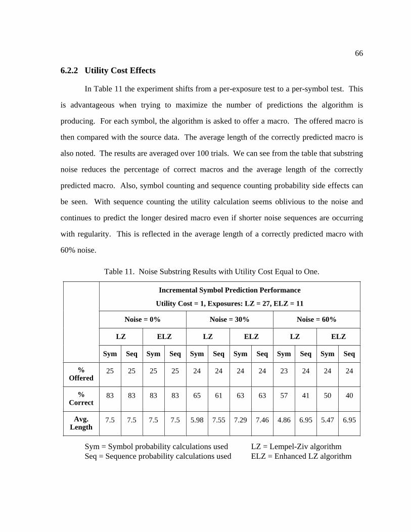
66
6.2.2 Utility Cost Effects
In Table 11 the experiment shifts from a per-exposure test to a per-symbol test. This
is advantageous when trying to maximize the number of predictions the algorithm is
producing. For each symbol, the algorithm is asked to offer a macro. The offered macro is
then compared with the source data. The average length of the correctly predicted macro is
also noted. The results are averaged over 100 trials. We can see from the table that substring
noise reduces the percentage of correct macros and the average length of the correctly
predicted macro. Also, symbol counting and sequence counting probability side effects can
be seen. With sequence counting the utility calculation seems oblivious to the noise and
continues to predict the longer desired macro even if shorter noise sequences are occurring
with regularity. This is reflected in the average length of a correctly predicted macro with
60% noise.
Table 11. Noise Substring Results with Utility Cost Equal to One.
Incremental Symbol Prediction Performance
Utility Cost = 1, Exposures: LZ = 27, ELZ = 11
Noise = 0% Noise = 30% Noise = 60%
LZ ELZ LZ ELZ LZ ELZ
Sym Seq Sym Seq Sym Seq Sym Seq Sym Seq Sym Seq
%Offered
25 25 25 25 24 24 24 24 23 24 24 24
%Correct
83 83 83 83 65 61 63 63 57 41 50 40
Avg.Length
7.5 7.5 7.5 7.5 5.98 7.55 7.29 7.46 4.86 6.95 5.47 6.95
Sym = Symbol probability calculations used LZ = Lempel-Ziv algorithm
Seq = Sequence probability calculations used ELZ = Enhanced LZ algorithm

67
Note in particular in Table 11 that the percentage correct is not 100% with zero noise.
To explain this phenomenon recall Table 4 and Table 5 on pages 55 and 55 respectively.
There are actually two contexts in the simulation sequence that are identical. Note in Table 5
the sequence “app z 3” followed by “desktop”. As we see in line three, “z” can take on
values from one to nine. When z = 1 then this is one context. Also note in Table 4 “app 1 3”
is followed by the topmost “desktop” in Table 5. This is the second duplicate context. Since
the contexts duplicate, the longer macro of interest is being predicted erroneously when the
second context occurs.
Finally with Table 12 and Table 13 the effect of utility cost values of three and five
are compared to the utility cost value of one in Table 11. The symbol probability calculation
seems to have additional merit over the sequence probability calculation. With the symbol
probability calculation, as the utility cost value is increased the percentage of correctly
predicted macros increases and the number of macros offered decreases. With the sequence
probability calculation, the utility cost value has no significant effect.
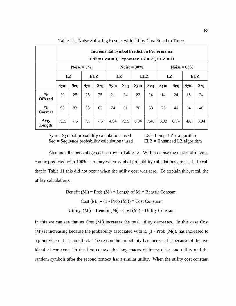
68
Table 12. Noise Substring Results with Utility Cost Equal to Three.
Incremental Symbol Prediction Performance
Utility Cost = 3, Exposures: LZ = 27, ELZ = 11
Noise = 0% Noise = 30% Noise = 60%
LZ ELZ LZ ELZ LZ ELZ
Sym Seq Sym Seq Sym Seq Sym Seq Sym Seq Sym Seq
%Offered
20 25 25 25 21 24 22 24 14 24 18 24
%Correct
93 83 83 83 74 61 70 63 75 40 64 40
Avg.Length
7.15 7.5 7.5 7.5 4.94 7.55 6.84 7.46 3.93 6.94 4.6 6.94
Sym = Symbol probability calculations used LZ = Lempel-Ziv algorithm
Seq = Sequence probability calculations used ELZ = Enhanced LZ algorithm
Also note the percentage correct row in Table 13. With no noise the macro of interest
can be predicted with 100% certainty when symbol probability calculations are used. Recall
that in Table 11 this did not occur when the utility cost was zero. To explain this, recall the
utility calculations.
Benefit (Mi) = Prob (Mi) * Length of Mi * Benefit Constant
Cost (Mi) = (1 - Prob (Mi)) * Cost Constant.
Utilityi (Mi) = Benefit (Mi) - Cost (Mi) – Utility Constant
In this we can see that as Cost (Mi) increases the total utility decreases. In this case Cost
(Mi) is increasing because the probability associated with it, (1 - Prob (Mi)), has increased to
a point where it has an effect. The reason the probability has increased is because of the two
identical contexts. In the first context the long macro of interest has one utility and the
random symbols after the second context has a similar utility. When the utility cost constant
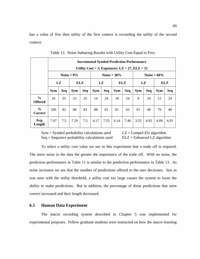
69
has a value of five then utility of the first context is exceeding the utility of the second
context.
Table 13. Noise Substring Results with Utility Cost Equal to Five.
Incremental Symbol Prediction Performance
Utility Cost = 5, Exposures: LZ = 27, ELZ = 11
Noise = 0% Noise = 30% Noise = 60%
LZ ELZ LZ ELZ LZ ELZ
Sym Seq Sym Seq Sym Seq Sym Seq Sym Seq Sym Seq
%Offered
16 25 23 25 14 24 18 24 9 24 12 24
%Correct
100 83 88 83 88 61 81 63 91 40 79 40
Avg.Length
7.07 7.5 7.29 7.5 4.17 7.55 6.14 7.46 3.55 6.92 4.09 6.91
Sym = Symbol probability calculations used LZ = Lempel-Ziv algorithm
Seq = Sequence probability calculations used ELZ = Enhanced LZ algorithm
To select a utility cost value we see in this experiment that a trade off is required.
The more noise in the data the greater the importance of the trade off. With no noise, the
prediction performance in Table 11 is similar to the prediction performance in Table 13. As
noise increases we see that the number of predictions offered to the user decreases. Just as
was seen with the utility threshold, a utility cost too large causes the system to loose the
ability to make predictions. But in addition, the percentage of those predictions that were
correct increased and their length decreased.
6.3 Human Data Experiment
The macro recording system described in Chapter 5 was implemented for
experimental purposes. Fellow graduate students were instructed on how the macro learning

70
system works and shown a few macro creation examples. The demonstration consisted of a
button sequence, or a button and key sequence, (the macro) followed by unrelated desktop or
application mouse clicking’s. In the demonstration, the sequence was repeated three times
and shown that the system identified the desired sequence and was able to play it back to the
user. The students were then asked to:
Create macros they felt might be useful for them
Create macros with a length ranging from three to six actions long
Teach the macro to the system as demonstrated
Teach the system until the number of macro exposures was twice the length of
the desired macro
Each student’s macro creation task is considered a trial and the results of the eight
trials are shown in Figure 24 and Figure 25. There were trials of four, seven, eight, and ten,
and eleven symbols. In many cases students succeeded in creating the macro they desired.
In other cases problems would come into play and hinder successful creation. Figure 24
shows the per-exposure results and enables us to view how well the desired sequence was
reflected into dictionary tree.
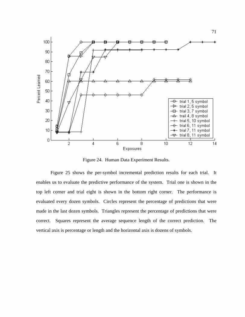
71
Figure 24. Human Data Experiment Results.
Figure 25 shows the per-symbol incremental prediction results for each trial. It
enables us to evaluate the predictive performance of the system. Trial one is shown in the
top left corner and trial eight is shown in the bottom right corner. The performance is
evaluated every dozen symbols. Circles represent the percentage of predictions that were
made in the last dozen symbols. Triangles represent the percentage of predictions that were
correct. Squares represent the average sequence length of the correct prediction. The
vertical axis is percentage or length and the horizontal axis is dozens of symbols.
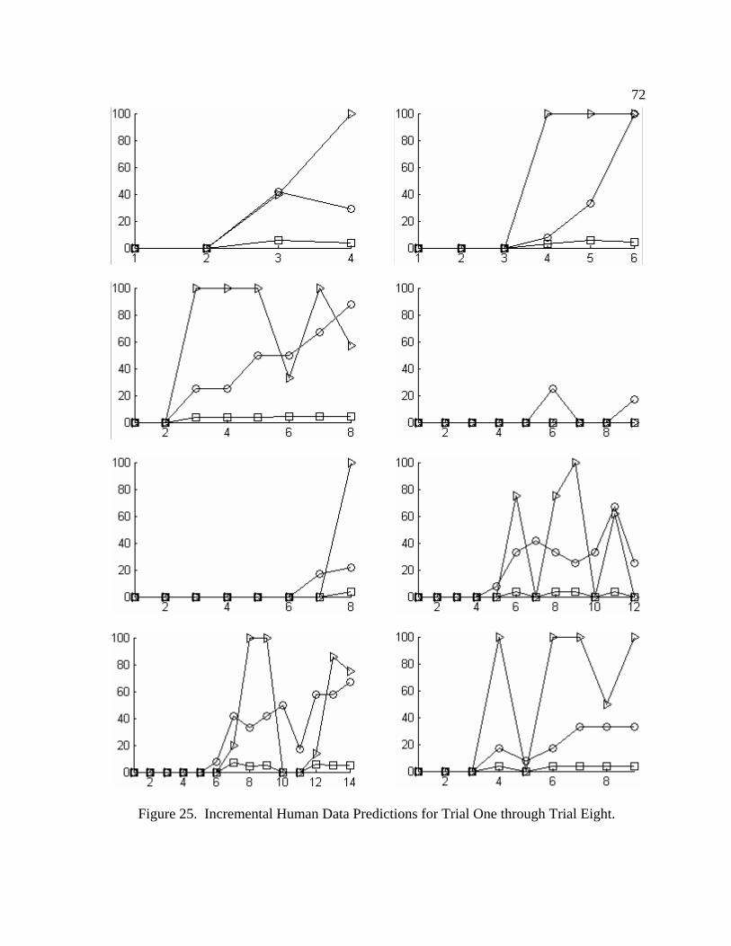
72
Figure 25. Incremental Human Data Predictions for Trial One through Trial Eight.
73
6.3.1 Analysis
Analysis of the trial data reveals several problem sources. The fundamental problem
is that symbols that needed to match for branch construction did not. Recall the coordinate
parameter in the symbol table list shown in Table 2 on page 35. Because the user did not
exactly repeat click button coordinates on each exposure, symbols were not matched. The
algorithm allowed a coordinate tolerance of 70 horizontal pixels and 50 vertical pixels. Not
all buttons are this small. Many buttons are much larger or are oblong shaped. This is
especially true for Web browser hyperlinks. Hyperlinks are often short, wide, and definitely
do not have a fixed size.
Recall that in Table 3 the expectation is that a macro can be learned and predicted in
as few as three exposures. For the human data experiment shown in Figure 24 this occurred
in one of the eight trials. This trial was of a five symbol macro and is listed first in the
figure’s legend. Also shown are two macros which were learned and predicted in four
exposures.
In two trials, no learning progress can be seen after a few exposures. For these cases,
the problem can be primarily attributed to button size variations. Specifically, the width of
hyperlinks can be very wide.
A more detailed post mortem indicates additional problem manifestations. One
problem relates to suffix substrings. Specifically, in most of the cases where the macro was
not learned in a short number of exposures, sequences that were suffixes of the desired macro
were learned. That is, if the macro was not learned in say the fifth exposure then a suffix of
the desired macro might have been offered to the user mid way through the fifth exposure.
This occurred because of dictionary tree fragmenting where the dictionary algorithm reset to
the root node at an inopportune time. Fragments of the desired macro can be seen in the left
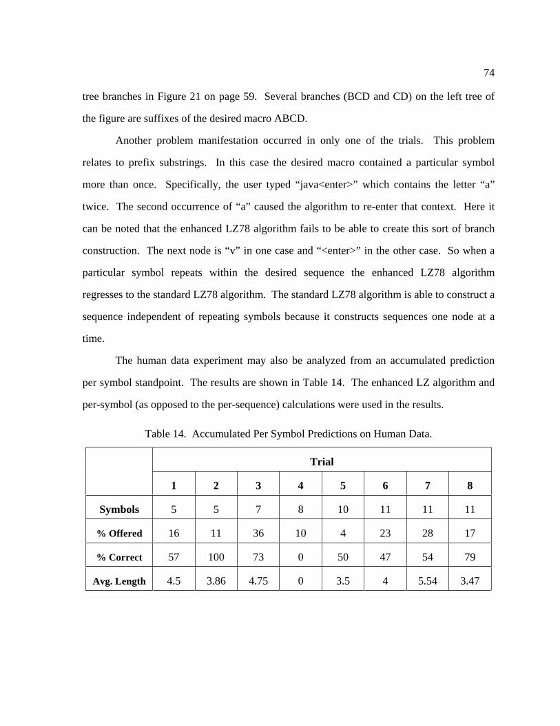
74
tree branches in Figure 21 on page 59. Several branches (BCD and CD) on the left tree of
the figure are suffixes of the desired macro ABCD.
Another problem manifestation occurred in only one of the trials. This problem
relates to prefix substrings. In this case the desired macro contained a particular symbol
more than once. Specifically, the user typed “java<enter>” which contains the letter “a”
twice. The second occurrence of “a” caused the algorithm to re-enter that context. Here it
can be noted that the enhanced LZ78 algorithm fails to be able to create this sort of branch
construction. The next node is “v” in one case and “<enter>” in the other case. So when a
particular symbol repeats within the desired sequence the enhanced LZ78 algorithm
regresses to the standard LZ78 algorithm. The standard LZ78 algorithm is able to construct a
sequence independent of repeating symbols because it constructs sequences one node at a
time.
The human data experiment may also be analyzed from an accumulated prediction
per symbol standpoint. The results are shown in Table 14. The enhanced LZ algorithm and
per-symbol (as opposed to the per-sequence) calculations were used in the results.
Table 14. Accumulated Per Symbol Predictions on Human Data.
Trial
1 2 3 4 5 6 7 8
Symbols 5 5 7 8 10 11 11 11
% Offered 16 11 36 10 4 23 28 17
% Correct 57 100 73 0 50 47 54 79
Avg. Length 4.5 3.86 4.75 0 3.5 4 5.54 3.47
75
Here we see in the table that the two tests which offered the greatest percentage of
macros were trails three and seven. As we see in Figure 24 for those two tests, the desired
macro was learned before the conclusion of the test. Another note is the eight symbol trial
four test in the table. Trial four had zero correct predictions. In Figure 24 we notice that this
test showed the least amount of learning at the conclusion of the test. One novelty is trial
two, the second five symbol test. Predictions were only made on 11% of the symbols yet the
predictions where 100% correct. By examining Figure 25, we see that for this case, the
desired macro was learned and could be predicted effectively.
Note the wild deviation in the correct prediction percentage values in trials six and
seven of Figure 25. Detailed analysis of the data around ten dozen symbols indicates that
there were predictions and the predictions were wrong. The reason for this could be the
imprecise ability to capture user actions with the experimental system used. On some macro
expressions, a similar almost duplicate symbol branch would be created instead of following
an existing branch. The mechanics of this issue are outlined in the following section, section
6.3.2. It is quite possible that the predictions might well have performed the correct actions
had the actions been played by the user. Note that predictions near the beginning of an
experiment are better. This would be explained by the fact that there are no similar almost
duplicate branches at the beginning of a test.
6.3.2 Generic Problems
The failure for the algorithm to learn macros after a short number of exposures can be
attributed to any one of several situational problems. Those problems that bore out from the
tests, and others that come to mind, are listed here.
One problem is window size consistency. When a window is resized, sequences in
the dictionary tree can suddenly become incorrect. Examples include the: minimize,
76
maximize, and close buttons. These buttons are in one location with one window width and
in another location with a different window width.
Another problem, related to coordinates, is window scroll bars. A vertical scroll bar
is typically very tall and narrow. Anywhere on the scroll bar can be clicked for a page up or
page down operation. Also the tab on the scroll bar can be dragged anywhere along the
length of the bar. These “anywhere” mouse operations are normally not duplicated by the
user regardless of the number of exposures. The same is true for horizontal scroll bars.
Dropdown text selection boxes are another problem. In a dropdown box the user
clicks or types in a text box and a new selection window appears just below the current text
box. The list can be context sensitive which causes a different list to be generated on
different occasions. The list variations prevent macro record and play consistency of
dropdown text boxes.
Application toolbars is another problem. Many applications allow for a
customization of toolbar organization. If the organization changes between exposures then
any sequences related to the toolbar buttons are suddenly completely incorrect in the
dictionary tree.
A solution to some of these problems may be possible though. If the macro learning
algorithm were embedded in the operating system then applications could be monitored more
succinctly. That is, the operating systems Inter Process Communication (IPC) messages may
be more revealing to state change then mouse and keyboard actions.
77
CHAPTER 7
CONCLUSION
In this work we examined a macro recording system. The system is capable of
learning the repetitive habits of a PC user on his desktop. Because action and state visibility
is required outside the realm of a single application such a system must be integral to the
operating system. Some sort of “hooking” into the operating system’s GUI is necessary.
As a learning algorithm we employed the Lempel-Ziv LZ78 algorithm as a sequence
prediction model. One problem with the Lempel-Ziv algorithm is its slow learning rate. To
improve the learning rate we added a set of three new algorithmic rules. These rules
enhanced the algorithm by increasing the learning rate. Finally, we saw that a population of
possible macros can be formed using PPM context prediction techniques and then examining
the dictionary sub trees for macro end points.
The macro learning system, and related algorithms, was designed to work at the PC
desktop level. Learned macros should be offered to the user when the user’s desktop context
repeats. The user then has the discretion to play the macro. Playing a macro is automation
for the user and an increased level of automation allows the user to work more productively.
Some of the significant windows related problems revealed in this research may be
worth addressing in future research. These include (1) learning button locations, and (2)
evaluating the graphics underneath each mouse click action. If these issues were addressed
the predictive accuracy of a macro learning system would be expected to increase
significantly.

78
One byproduct of this work is the realization that the learning algorithm could be
encapsulated, as a class, for generic use. The Lempel-Ziv algorithm could be applied to a
variety of learning problems. For each application, symbol parameters can be defined in
accordance with the problem constraints. The learning algorithm’s performance could be
refined and optimized apart from its intended application.
Another byproduct of this work is that a similar form of learning could be extended to
WWW search engines. It may be possible that Web page ranking can be improved by
monitoring and learning Web navigation. That is to say, learning the association between (1)
a specific text query, and (2) discovering a specific web page may be a very valuable
association for a Web search engine.
79
BIBLIOGRAPHY
[1] A. Cypher, "EAGER: Programming Repetitive Tasks by Example", Proceedings of the
SIGCHI conference on Human factors in computing systems: Reaching through
technology, Page 33 - 39, March 1991.
[2] P. Gorniak and D. Poole, "Predicting Future User Actions by Observing Unmodified
Applications", Proceedings of the Seventeenth National Conference on Artificial
Intelligence and Twelfth Conference on Innovative Applications of Artificial
Intelligence, Page 217 - 222, July 2000.
[3] B. Davison and H. Hirsh, "Predicting Sequences of User Actions", Proceedings of the
1998 AAAI/ICML Workshop, Page 5 - 12, 1998.
[4] H. Hirsh and B. Davison, "An adaptive UNIX command-line assistant", Proceedings of
the first international conference on Autonomous agents, Page 542 - 543, February
1997.
[5] A. Sugiura and Y. Koseki, "Simplifying Macro Definition in Programming by
Automation", Proceedings of the 9th annual ACM symposium on User interface
software and technology, Page 173 – 182, November 1996.
[6] D. Kurlander and S. Fiener, "A history-based macro by example system", Proceedings
of the 5th annual ACM symposium on User interface software and technology, Page 99
– 106, December 1992.
[7] D. Appleman, "Visual Basic Programmer's Guide to the Win32 API", Sams Publishing,
Chapters 5 – 6, 1999.
[8] S. Robinson, "Advanced .NET Programming", Wrox Press, Chapter 6, 2002.
80
[9] S. Teilhet, “Subclassing & Hooking”, O’Reilly & Associates, 2001.
[10] M. Feder, N. Merhav, and M. Gutman, “Universal Prediction of Individual Sequences”,
IEEE Transactions on Information Theory, Volume 38, Issue 4, Page 1258 – 1270, July
1992.
[11] J. Ziv and A. Lempel, "Compression of Individual Sequences via Variable-rate
Coding", IEEE Transactions on Information Theory, Volume 24, Issue 5, Page 530 –
536, September 1978.
[12] T. Bell, I. Witten and J. Cleary, "Modeling for Text Compression", ACM Computing
Surveys, Volume 21, Issue 4, Page 557–591, December 1989.
[13] A. Bhattacharya and S. Das, "LeZi-update: An Information-theoretic framework for
personal mobility tracking in PCS networks", Wireless Networks, Volume 8, Issue 2/3,
Page 121 – 135, March 2002.
[14] K. Gopalratnam and D. Cook, "Active Le-Zi: An Incremental Parsing Algorithm for
Sequential Prediction", Proceedings of the Florida Artificial Intelligence Research
Symposium, 2003.
[15] P. Sandanayake and D. Cook, “Imitating Agent Game Strategies Using a Scalable
Markov Model”, Proceedings of the Fifteenth International Florida Artificial
Intelligence Research Society Conference, Page 349 – 353, May 2002.
[16] S. Russell and P. Norvig, "Artificial Intelligence a Modern Approach”, Prentice Hall,
Page 5 – 6, 1995.
[17] I. Witten, A. Moffat and T. Bell, "Managing Gigabytes", Van Nostrand Reinhold,
Chapter 2, 1994.
81
BIOGRAPHICAL INFORMATION
Mr. Elliott received his Bachelor of Science in Electrical Engineering from the
University of Oklahoma, Norman Oklahoma. His areas of study included electronics, digital
design, data communications, and control systems.
After graduation, Mr. Elliott progressed in technical expertise to the level of Senior
Electronics Design Engineer. This occurred while employed at E-Systems Inc. which is now
known as L-3 Communications Corp. His work included numerous embedded
microprocessor designs for aircraft audio communication, control interface, and radar display
systems.
Mr. Elliott switched gears from hardware development to software development
when employed for Nortel Networks as a Member of Scientific Staff. His work included
switch and cell site software development for TDMA and GPRS technologies.
Recently Mr. Elliott received his Master of Science in Computer Science and
Engineering in December of 2004 from the University of Texas at Arlington. His areas of
study include artificial intelligence, prediction algorithms, neural networks, and genetic
algorithms.