laser desorption/ionization- tandem mass spectrometry...
TRANSCRIPT
1
LASER DESORPTION/IONIZATION- TANDEM MASS SPECTROMETRY OF
ANTHRAQUINONE DYES AND LEAD WHITE PIGMENT FOR PAINTED WORKS OF ART
By
MICHAEL PATRICK NAPOLITANO
A DISSERTATION PRESENTED TO THE GRADUATE SCHOOL OF THE UNIVERSITY OF FLORIDA IN PARTIAL FULFILLMENT
OF THE REQUIREMENTS FOR THE DEGREE OF DOCTOR OF PHILOSOPHY
UNIVERSITY OF FLORIDA
2013

2
© 2013 Michael Patrick Napolitano

3
To all the educators in my life who have inspired me
and nurtured my love of empiricism, science, and knowledge; and to the preservation and continuance
of the culture and heritage of the people of the Occident
4
ACKNOWLEDGMENTS
Certainly, I must first humbly extend my most sincere gratitude to my research
advisor, Dr. Richard Yost. The completion of my degree would not have been possible
without his unwavering support. As my life as a chemist develops, I shall hold inviolate
his advice and hope to demonstrate that his efforts have not been in vain. I am also
very grateful for the advice from and friendship of Dr. James Horvath. During our many
discussions in his office, he instilled in me the sense of forthrightness and pride an
educator must have. I thank my committee members Dr. John Eyler, Dr. Leonid Moroz,
Dr. Nicolo Omenetto, and Dr. David Powell for their patience and guidance. Thanks are
also given to Julie Arlsanoglu, Yelena Bobkova, Dr. Phil Brucat, Dr. Mari Prieto
Conaway, Dr. Ron Heeren, Dr. Jodie Johnson, Andras Kiss, Dr. Lennaert Klerk,
Dr. Katrien Kuene, Dr. Ping-Chung Kuo, Dr. Ben Smith, and Dr. Don Smith for all of
their assistance.
I thank all the fellow students and friends that have made my time at UF
memorable and have also provided stimulating, scientific discussions including, in
alphabetical order, Dr. Dodge Baluya, Dr. Stacey Benjamin, Dr. John Bowden, Dr. Tim
Garrett, Dr. Fabrizio Guzzetta, Chris Hilton, Dr. Lloyd Horne, Dr. Kaan Kececi,
Antoinette Knight, Dr. Rachelle Landgraf, Hillary Lathrop, Jessica Leigh, Dr. Dan
Magparangalan, Dr. Antonio Masello, Dr. Rob Menger, Funda Mira, Dr. Giovennella
Moscovici, Dr. David Pirman, Karla Radke, Dr. Rich Reich, Dr. Dave Richardson, Anna
Sberegaeva, Dr. Dosung Sohn, Dr. Jennifer Garrett Williams, and Dr. Alex Wu; with
particularly special attention to Dominic Colosi, Dr. Frank Kero, Whitney Stutts, and Dr.
Marilyn Prieto Tourné. Thanks to the two NSF-REU students, Vivian Estavam-Cornélio

5
and Jennifer Webber, who provided both assistance to my research and a platform to
hone my mentoring skills.
Finally, I want to thank my parents, family, and friends back home in New Jersey.
Their love and constant, unfaltering enthusiasm and support have sustained me during
my seemingly unending pursuit of higher education.
6
TABLE OF CONTENTS
page
ACKNOWLEDGMENTS .................................................................................................. 4
LIST OF TABLES ............................................................................................................ 8
LIST OF FIGURES .......................................................................................................... 9
ABSTRACT ................................................................................................................... 12
CHAPTER
1 INTRODUCTION .................................................................................................... 15
Cultural Heritage ..................................................................................................... 15
Conservation Science ............................................................................................. 16
Archaeometry ................................................................................................... 16
History of Conservation Science ...................................................................... 17
Methods of Analysis ......................................................................................... 18
Instrumentation ....................................................................................................... 20
Laser Desorption/Ionization .............................................................................. 20
Matrix-Assisted Laser Desorption/Ionization .................................................... 22
Electrospray Ionization ..................................................................................... 23
Linear Quadrupole Ion Trap ............................................................................. 25
Orbitrap ............................................................................................................ 26
Figures of Merit ................................................................................................ 28
Overview of Dissertation ......................................................................................... 30
2 TANDEM MASS SPECTROMETRY OF ANTHRAQUINONES ................................. 34
Background ............................................................................................................. 34
Experimental Methods ............................................................................................ 42
Chemicals and Materials .................................................................................. 42
Recrystallization of Standards .......................................................................... 42
Preparation of Chemicals ................................................................................. 43
Electrospray Ionization Parameters .................................................................. 44
Laser Desorption/Ionization and Matrix-Assisted Laser Desorption/Ionization Parameters ................................................................. 45
Ultraviolet–visible (UV) Light Exposure ............................................................ 47
Results and Discussion........................................................................................... 47
Electrospray Ionization of Anthraquinones ....................................................... 48
Laser Desorption/Ionization of Anthraquinones ................................................ 54
Matrix-Assisted Laser Desorption/Ionization of Anthraquinones ...................... 61
Conclusion .............................................................................................................. 64
7
3 TANDEM MASS SPECTROMETRY OF CLUSTERS FROM LEAD WHITE .......... 89
Background ............................................................................................................. 89
Experimental Methods .......................................................................................... 105
Chemicals and Materials ................................................................................ 105
Preparation of Chemicals ............................................................................... 105
Ionization and Instrumental Parameters ......................................................... 105
Results and Discussion......................................................................................... 107
Full-Scan Spectra Analysis ............................................................................. 107
Tandem Mass Spectrometric Analysis ........................................................... 112
Final Mass Assignments................................................................................. 115
Conclusion ............................................................................................................ 117
4 LASER DESORPTION/IONIZATION-TANDEM MASS SPECTROMETRY OF MADDER AND LEAD WHITE DIRECTLY FROM ARTISTIC SAMPLES .............. 136
Background ........................................................................................................... 136
Experimental Methods .......................................................................................... 139
Samples: Painting Fragments and Dyed Silk Swatches ................................. 139
Laser Desorption/Ionization Parameters ........................................................ 140
Instrumental Parameters ................................................................................ 141
Results and Discussion......................................................................................... 141
In Situ Detection of Alizarin from Painting Samples ....................................... 141
In Situ Detection of Madder from Swatches of Dyed Silk ............................... 142
In Situ Detection of Lead White from Painting Samples ................................. 145
Conclusion ............................................................................................................ 146
5 CONCLUSION AND FUTURE DIRECTIONS ....................................................... 161
Conclusions .......................................................................................................... 161
Future Directions .................................................................................................. 163
REFERENCES ............................................................................................................ 167
BIOGRAPHICAL SKETCH .......................................................................................... 177
8
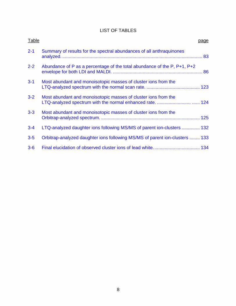
LIST OF TABLES
Table page 2-1 Summary of results for the spectral abundances of all anthraquinones
analyzed. ............................................................................................................ 83
2-2 Abundance of P as a percentage of the total abundance of the P, P+1, P+2 envelope for both LDI and MALDI. ..................................................................... 86
3-1 Most abundant and monoisotopic masses of cluster ions from the LTQ-analyzed spectrum with the normal scan rate. ......................................... 123
3-2 Most abundant and monoisotopic masses of cluster ions from the LTQ-analyzed spectrum with the normal enhanced rate. .......................... ...... 124
3-3 Most abundant and monoisotopic masses of cluster ions from the Orbitrap-analyzed spectrum. ............................................................................ 125
3-4 LTQ-analyzed daughter ions following MS/MS of parent ion-clusters .............. 132
3-5 Orbitrap-analyzed daughter ions following MS/MS of parent ion-clusters ........ 133
3-6 Final elucidation of observed cluster ions of lead white. ................................... 134
9
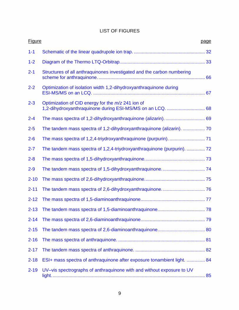
LIST OF FIGURES
Figure page 1-1 Schematic of the linear quadrupole ion trap. ...................................................... 32
1-2 Diagram of the Thermo LTQ-Orbitrap. ................................................................ 33
2-1 Structures of all anthraquinones investigated and the carbon numbering scheme for anthraquinone. ................................................................................. 66
2-2 Optimization of isolation width 1,2-dihydroxyanthraquinone during ESI-MS/MS on an LCQ. ..................................................................................... 67
2-3 Optimization of CID energy for the m/z 241 ion of 1,2-dihydroxyanthraquinone during ESI-MS/MS on an LCQ. ............................. 68
2-4 The mass spectra of 1,2-dihydroxyanthraquinone (alizarin). .............................. 69
2-5 The tandem mass spectra of 1,2-dihydroxyanthraquinone (alizarin). ................. 70
2-6 The mass spectra of 1,2,4-triydroxyanthraquinone (purpurin). ........................... 71
2-7 The tandem mass spectra of 1,2,4-triydroxyanthraquinone (purpurin). .............. 72
2-8 The mass spectra of 1,5-dihydroxyanthraquinone. ............................................. 73
2-9 The tandem mass spectra of 1,5-dihydroxyanthraquinone. ................................ 74
2-10 The mass spectra of 2,6-dihydroxyanthraquinone. ............................................. 75
2-11 The tandem mass spectra of 2,6-dihydroxyanthraquinone. ................................ 76
2-12 The mass spectra of 1,5-diaminoanthraquinone. ................................................ 77
2-13 The tandem mass spectra of 1,5-diaminoanthraquinone. ................................... 78
2-14 The mass spectra of 2,6-diaminoanthraquinone. ................................................ 79
2-15 The tandem mass spectra of 2,6-diaminoanthraquinone. ................................... 80
2-16 The mass spectra of anthraquinone. .................................................................. 81
2-17 The tandem mass spectra of anthraquinone. ..................................................... 82
2-18 ESI+ mass spectra of anthraquinone after exposure tonambient light. .............. 84
2-19 UV–vis spectrographs of anthraquinone with and without exposure to UV light. .................................................................................................................... 85
10
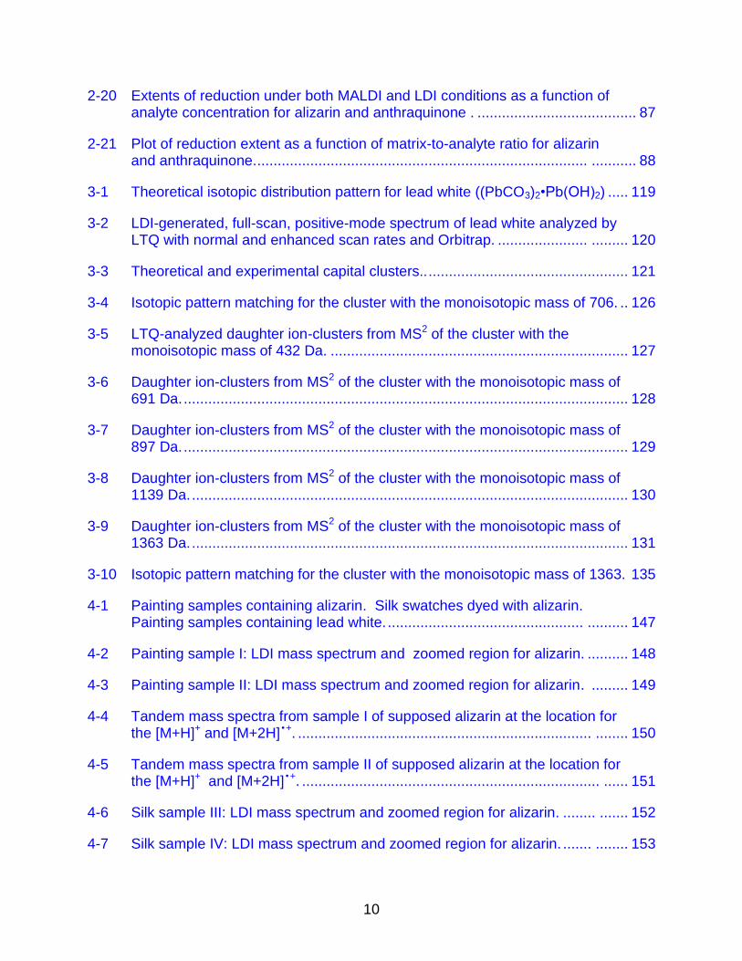
2-20 Extents of reduction under both MALDI and LDI conditions as a function of analyte concentration for alizarin and anthraquinone . ....................................... 87
2-21 Plot of reduction extent as a function of matrix-to-analyte ratio for alizarin and anthraquinone. ................................................................................. ........... 88
3-1 Theoretical isotopic distribution pattern for lead white ((PbCO3)2•Pb(OH)2) ..... 119
3-2 LDI-generated, full-scan, positive-mode spectrum of lead white analyzed by LTQ with normal and enhanced scan rates and Orbitrap. ...................... ......... 120
3-3 Theoretical and experimental capital clusters.. ................................................. 121
3-4 Isotopic pattern matching for the cluster with the monoisotopic mass of 706. .. 126
3-5 LTQ-analyzed daughter ion-clusters from MS2 of the cluster with the monoisotopic mass of 432 Da. ......................................................................... 127
3-6 Daughter ion-clusters from MS2 of the cluster with the monoisotopic mass of 691 Da. ............................................................................................................. 128
3-7 Daughter ion-clusters from MS2 of the cluster with the monoisotopic mass of 897 Da. ............................................................................................................. 129
3-8 Daughter ion-clusters from MS2 of the cluster with the monoisotopic mass of 1139 Da. ........................................................................................................... 130
3-9 Daughter ion-clusters from MS2 of the cluster with the monoisotopic mass of 1363 Da. ........................................................................................................... 131
3-10 Isotopic pattern matching for the cluster with the monoisotopic mass of 1363. 135
4-1 Painting samples containing alizarin. Silk swatches dyed with alizarin. Painting samples containing lead white. ................................................ .......... 147
4-2 Painting sample I: LDI mass spectrum and zoomed region for alizarin. .......... 148
4-3 Painting sample II: LDI mass spectrum and zoomed region for alizarin. ......... 149
4-4 Tandem mass spectra from sample I of supposed alizarin at the location for the [M+H]+ and [M+2H] •+. ........................................................................ ........ 150
4-5 Tandem mass spectra from sample II of supposed alizarin at the location for the [M+H]+ and [M+2H] •+. ......................................................................... ...... 151
4-6 Silk sample III: LDI mass spectrum and zoomed region for alizarin. ........ ....... 152
4-7 Silk sample IV: LDI mass spectrum and zoomed region for alizarin. ....... ........ 153
11
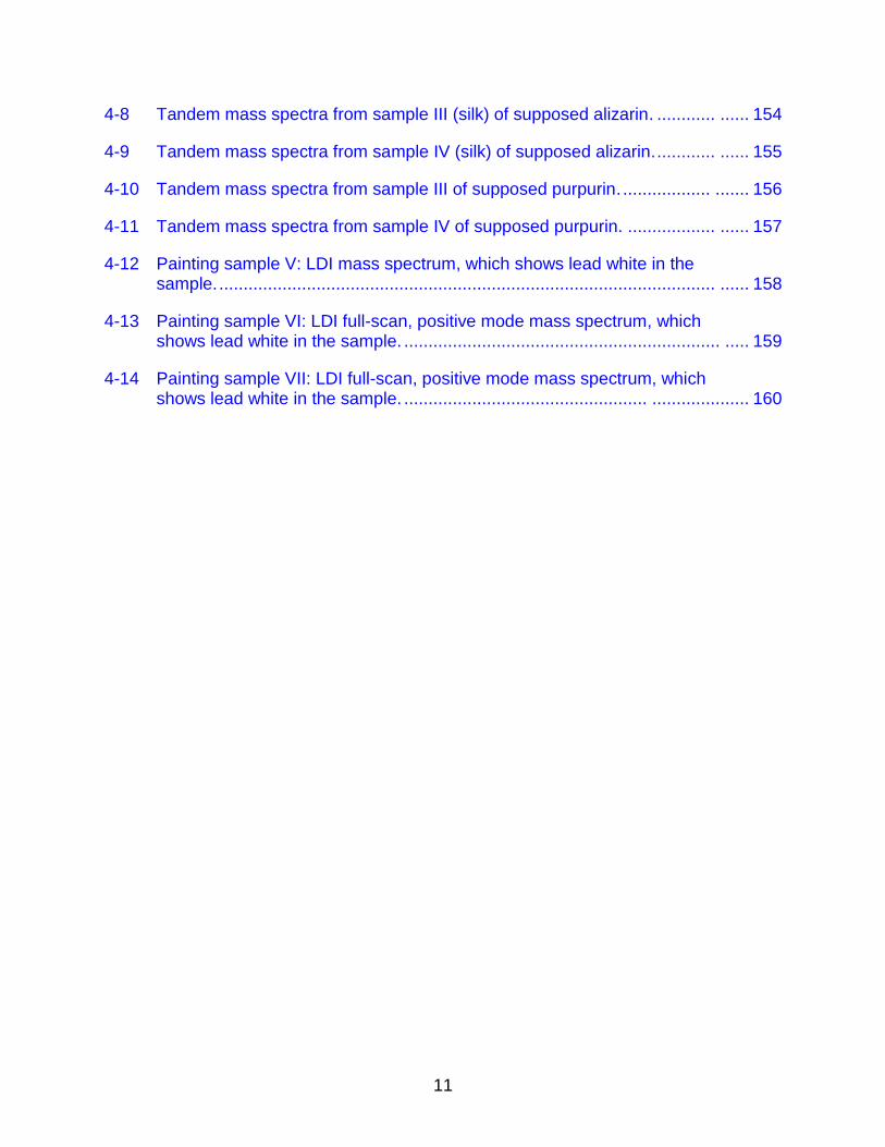
4-8 Tandem mass spectra from sample III (silk) of supposed alizarin. ............ ...... 154
4-9 Tandem mass spectra from sample IV (silk) of supposed alizarin. ............ ...... 155
4-10 Tandem mass spectra from sample III of supposed purpurin. .................. ....... 156
4-11 Tandem mass spectra from sample IV of supposed purpurin. .................. ...... 157
4-12 Painting sample V: LDI mass spectrum, which shows lead white in the sample. ...................................................................................................... ...... 158
4-13 Painting sample VI: LDI full-scan, positive mode mass spectrum, which shows lead white in the sample. ................................................................. ..... 159
4-14 Painting sample VII: LDI full-scan, positive mode mass spectrum, which shows lead white in the sample. .................................................. .................... 160
12
Abstract of Dissertation Presented to the Graduate School of the University of Florida in Partial Fulfillment of the Requirements for the Degree of Doctor of Philosophy
LASER DESORPTION/IONIZATION-
TANDEM MASS SPECTROMETRY OF ANTHRAQUINONE DYES AND LEAD WHITE PIGMENT FOR PAINTED WORKS OF ART
By
Michael Patrick Napolitano
August 2013
Chair: Richard A. Yost Major: Chemistry
The goal of sustaining cultural heritage is manifested by diagnosing and
preserving objects of historical and corporeal significance and artistic beauty. To
achieve this goal, conservation scientists develop and use methods commensurate with
new technologies of traditional analytical chemists. For instance,
gas-chromatography/mass spectrometry (GC/MS) has been extensively used for many
years for the characterization of oil-painting components; however, this method often
requires derivatization, cannot be used for direct surface analyses, and, most
importantly, is destructive. Consequently, laser desorption/ionization (LDI) and
matrix-assisted laser desorption/ionization (MALDI) MS have been gaining popularity
and interest among the conservation community for their non-destructiveness and ability
to interrogate intact surfaces. Furthermore, the single quadrupole mass analyzer of
most GC/MS instruments and the time-of-flight (ToF) mass analyzer of most LDI and
MALDI instruments lack the capability of tandem MS (MS/MS and in general MSn),
13
which is a powerful attribute available on a linear quadrupole ion trap (LIT) to provide
unambiguous structural identification of known and unknown dye and pigment
components of a painted work of art.
This work will present three projects for the analysis of painted works of art that
used both LDI and MALDI-MS on an LIT and Orbitrap, which have been conducted in
collaboration with The Metropolitan Museum of Art, New York. The first project
examined the peculiar ionization of anthraquinone dyes such as alizarin. For instance,
when ionized by either LDI or MALDI, alizarin (MW = 240) exhibited a dominant ion of
[M+2H]+ at m/z 242—with a far greater abundance than the expected ion of [M+H]+ at
m/z 241. For the first time, MS2 analysis of these anomalous [M+2H]+ ions suggested a
laser-induced reduction of one of the anthraquinone’s carbonyl groups, as well as
different relative abundances of neutral losses from either water or ammonia, depending
upon those functional groups’ proximity to the reduced carbonyl.
The second project involved the elucidation of formulae from a suite of
isotopically complex cluster ions from the artists’ pigment lead white,
(PbCO3)2·Pb(OH)2. Using LDI on both an LIT and Orbitrap, the low- and high-resolution
full- and tandem-mass spectra were used in concert with deductive and inductive
reasoning to decipher the peculiar spectra. The results are reported for the first time
and may contribute to a conservation scientist’s ability to rapidly identify a pigment
ubiquitous since antiquity.
The third project employed the results from the above two projects to directly
detect the red anthraquinone dyes alizarin and purpurin and the white pigment lead
white in various artistic samples. For the first time, the LDI-MS2 detection of alizarin and
14
madder was achieved in both paintings and textiles and the LDI-MS detection of lead
white was achieved in paintings, all without any sample pretreatment whatsoever.
The results described herein provide new insight into a unique ionization
phenomenon found in a specific class of dye molecules, have elucidated the isotopically
complex cluster ions formed from a common pigment, and have shown the detection of
those dyes and pigment in artistic samples. Moreover, these results offer new avenues
for the conservation science community to diagnose—and ultimately preserve—painted
works of art for the defense of cultural heritage.
15
CHAPTER 1 INTRODUCTION
Cultural Heritage
A proper grammar on the notion of cultural heritage and the science applied to
that notion must first be established before any meaningful logic or rhetoric may ensue.
After all, the term heritage may have difficulty being either accurately or precisely
defined in the lexicon of either scientists or the general population. The United Nations
Educational, Scientific and Cultural Organization (UNESCO) established a convention in
1972 regarding world cultural and natural heritage’s definition, threat of damage and
destruction, need for economic and scientific investment, and requisite of diffused and
increased knowledge thereof.1 UNESCO’s convention explicitly defined cultural
heritage to include monuments, such as works of architecture, monumental sculpture
and painting, inscriptions, and cave dwellings; groups of buildings; and sites; which are
of outstanding universal value from the point of view of history, art, or science. However
inclusive UNESCO’s convention may seem, it is obviously intended to protect grand
structures, with possible political or economic overtures, and never mentions painted
works of art. Cultural heritage was succinctly defined by Ciliberto in the introductory
chapter of his excellent text as the whole of human cultural patrimony, which is
everything that refers to the history of civilization and may include all works and
documents that are of value from an archaeological, historical, or artistic perspective.2
For the purpose of this dissertation, cultural heritage will be exemplified by painted
works of art whose appreciation is embraced by the public and whose need for analysis
is growing among archaeometrists, conservation scientists, and analytical chemists.
16
Conservation Science
The orthodoxy of contemporary science regrettably perpetuates the atomization
of fields to the unfortunate exclusion of comprehensive disciplinary approaches and the
hierarchical stratification of fields and subfields. Such hypercategorization of fields may
be exemplified by the analysis of painted works of art presented in this dissertation,
which may simultaneously be described broadly as “materials science” and specifically
as “diagnostic conservation science”. To understand this seemingly disparate
nomenclature, its grammatical and historical context must first be addressed.
Archaeometry
Conservation science is defined in the introductory chapter of Artioli’s elementary
text and it is traced back to the broader fields whence it came.3 ”Materials science” is
considered to be the highest strata, a field so vast that a concise definition may not be
readily applied. Thereafter, “archaeometry” follows, which may be defined as the
“quantification and physiochemical analyses of archaeological materials”.4
Archaeometry may be a sufficient term to describe the majority of related work
conducted under its umbrella; nevertheless, it is then divided into 1) “archaeology” and
2) “conservation science”.
Archaeology seeks to “understand past societies from their surviving cultural
materials”3, which is accomplished by dating via physical and chemical methods4, and
studying how artifacts were obtained4, used4, traded3, and distributed3. One common
misconception is that archaeology is restricted to the realm of qualitative methodologies,
but dating methods, such as the exploitation of carbon-14 dating achieved by
accelerator mass spectrometry (AMS), certainly negate that notion.
17
Conservation science is used to diagnose, authenticate, and preserve artifacts,
objects, and works of art for the purposes of curatorship, art history, and museum
conservation and restoration, thereby making it distinct from archaeology.3 Artioli
cleverly describes conservation science as acting with respect to a function of time, that
is, “chemical kinetics related to the human time-scale”.3 Consideration must be given to
an object’s original processing and construction, present condition, and future alteration
via degradation processes.3 Conservation science is practically employed by dating,
characterizing (analyzing), and establishing provenance and original usage of materials
and objects, and consequently identifying and preventing degradation of materials and
objects.2,3 Overall, archaeology may be considered as the attempt to understand the
totality of an object’s history and context, whereas conservation science may be used to
operate on an object for analyses and preservation.
History of Conservation Science
Though conservation science has recently been steadily gaining recognition as
an independently viable and legitimate field, when considered separately from the
distinction of its field-label, it may be seen as simply the application of chemistry and
other natural sciences that have been conducted since the early days of modern
science, as detailed in a interesting survey by Caley5. For instance, Klaproth
determined the metallic composition of Greek and Roman coins using gravimetry ca.
1795, Chaptal published the first ever qualitative analysis of the chemical composition of
ancient pigments in 1809, Humphry Davy examined ancient pigments of Rome and
Pompeii in 1815, Faraday studied for the first time the use of lead in glazes of Roman
pottery ca. 1867, and Kekulé analyzed ancient samples of wood tar that may have
contained benzene-derived compounds.4,5 Moreover, not until the early 1950s was the
18
term archaeometry was first coined, with an eponymous journal launched in 1958.3,4
The Journal of Archaeological Science was started in 1974, but it should be noted that
articles on conservation science are often found in traditional journals of analytical
chemistry.
Though conservation science might be perceived as an ancillary research field, it
has long been popular, as with the Georgian and Victorian era’s contemporaries noted
above. The field has taken root in several museums and some universities;
independent departments for conservation science are commonly housed in the former,
but only rarely in the latter. Many of the most notable conservation science laboratories
coincide with their host museum’s prestige, with some exceptions. Some museums in
the United States with dedicated conservation science departments or laboratories are
(with the year a department or laboratory was established, if known): The Museum of
Fine Arts Boston (1930s), The National Gallery of Art (1950), The Smithsonian
Institution (1963), The J. Paul Getty Museum (1985), The Art Institute of Chicago
(2003), The Indianapolis Museum of Art (2008), Winterthur, and The Metropolitan
Museum of Art. By far, the most prolific and well-known department is the Getty
Conservation Institute at the Getty Museum. Some examples of U.S. colleges or
universities with academic departments in conservation are The University of Delaware,
Buffalo State College, Scripps College, and New York University, though they primarily
teach preservation and not scientific analysis.
Methods of Analysis
As noted above, diagnostic conservation science may be considered subordinate
to materials science and, more relevant to this dissertation, analytical chemistry.
Therefore, virtually all analytical instrumentation and methodologies can be—and
19
indeed have already been—employed for the chemical diagnosis of works of art and
other artifacts and objects. To provide a historical or literature review of the various
types of instrumentation and their myriad range of applications would be unnecessarily
cumbersome. Instead, the reader is directed to the introductory sections in Chapters 2,
3, and 4 of this dissertation for thorough reviews of the analytical methods relevant to
the topics in those Chapters.
Critical to the analysis of objects, artifacts, and works of art is the extent of
destructiveness. Three categories of destructiveness are considered, which are, in
order of increasing degree of destructiveness: non-invasive, non-destructive, and
micro-destructive.2 Non-invasive techniques require no sampling of the object and
leave the object unaltered; examples include micro-X-ray fluorescence on a medieval
painted wooden reliquary6 and micro-Raman spectroscopy for an overpainted
reproduction of a Byzantine icon7. Non-destructive techniques require sampling of the
object, yet the sample can be analyzed by succeeding methods; examples include laser
ablation-inductively coupled plasma-MS of ancient African glass beads8 and
time-of-flight (ToF) secondary ion MS of ancient Tuscan ceramics9. Micro-destructive
techniques require minimal sampling of the object and completely destroy or consume
the sample; examples include pyrolysis-gas chromatography/MS of the coating on an
Oriental lacquered wooden dish10 and direct temperature-resolved MS of organic
residues in Roman-era pottery11. Laser desorption/ionization MS is an example of a
non-destructive technique, and will be thoroughly reviewed in the following Chapters,
particularly Chapter 4. It is the primary means of analysis for the work presented in this
dissertation and its theory and instrumentation shall henceforth be explained.
20
Instrumentation
A mass spectrometer may be conceived to be primarily constructed of three
main, sequential components: 1) ionization source, 2) mass analyzer, and 3) detector.
Early mass spectrometers displayed and recorded spectra on a phosphorescent screen
or a photographic plate. Since the adoption of the microprocessor and the personal
computer, it is quite appropriate to consider a computational/processing unit as a fourth
component. The research presented in this dissertation may be classified as applied
mass spectrometry that ventures into the realm of fundamentals, particularly those
related to ionization. Therefore, the following section shall be presented in a manner
proportional to that of the research. For instance, topics on ionization will include laser
desorption/ionization (LDI), matrix-assisted laser desorption/ionization (MALDI), and
electrospray ionization (ESI); topics on mass analyzers will include the linear
quadrupole ion trap (LIT), and orbital trap (Orbitrap). For thorough reviews of the
literature regarding the precedent of research and historical perspective of the
instrumentation used that is specific to the three projects in this dissertation, the reader
is directed to the introductory sections of the Chapters for those respective projects.
Laser Desorption/Ionization
Soon after the laser was developed in the late 1950s, it was first employed as an
ionization source for a (double focusing) mass spectrometer in 1963 by Honig and
Woolston12. Although the instrument suffered from low spectral resolution from
space-charge effects and low (ppm) sensitivity (that is, to current standard), it was able
to detect singly charged ions from metals, semiconductors, and insulators. Using an arc
discharge just after the sample stage, the instrument was, in effect, also the first to
21
produce singly and doubly charged ions with both laser ablation and electron ionization
(EI).
In 1966, a laser was first coupled to a time-of-flight (ToF) mass analyzer, which
was used for the analysis of metal foils and organic compounds, though only atoms, not
molecular ions, were observed from the latter.13 The mechanism of ionization was
considered to be a result of thermionic electrons being released following the laser
heating the sample, a theory repeated14 without proof for many years afterwards.
Interestingly, the authors comment on the importance and difficulty of finding the “right
laser power for a…sample” to find a balance between low signal and high background—
a feature still well-known to present-day users of an LDI source. The first successful
generation of intact ions using LDI (with a ToF) from organic compounds was reported
in 1970.15 LDI-generated molecular ions are typically comprised of either odd-electron
radical ions ([M] •+) or even-electron ions ([M+H]+ or [M+Z]+, where Z = metal cation).
The prior developments reached a practical conclusion with the 1975 introduction
of the laser microprobe mass analyzer (LAMMA) by Hillenkamp and Kaufmann, which
was able to achieve both high spatial resolution (0.5 μm) through the simple use of a
microscope objective to focus the laser beam and slightly increased sensitivity
(0.4 ppm).16 Hillenkamp’s instrument was the direct influence for the first
commercialized laser-based mass spectrometer, the LAMMA-500, and was primarily
used for probing thin-sliced tissue sections that were embedded in a matrix of polymer
resin.14,17 Indeed, it was “the sensitivity-limiting ‘noise’” resulting from that polymer resin
that contributed to the discovery of the MALDI principle.17
22
Matrix-Assisted Laser Desorption/Ionization
MALDI evolved not only from LDI, but from other “soft” ionization methods that
form gas-phase molecular ions with neither excessive fragmentation nor prior
evaporation.17,18 Such “desorption” methods include field desorption (FD), developed in
196919; plasma desorption (PD), developed in 197420; static secondary-ion MS (SIMS),
developed in 197821; and fast atom bombardment (FAB), developed in 198122. Much
like the polymer resin used with LAMMA, the glycerol matrix used with FAB also
contributed to the MALDI principle.17 The significant difference with MALDI, compared
to the just-mentioned ionization methods, is MALDI’s relatively soft ionization event that
minimizes source fragmentation, creating primarily singly-charged ions, and allowing
ionization of (biological) molecules in excess of 100,000 Da.17
MALDI’s desorption and ionization energy is first obtained via photons from a
laser that are absorbed by an infrared- or ultraviolet (UV)-absorbing matrix, typically an
organic acid of low molecular weight; two of the most commonly used are
2,5-dihydroxybenzoic acid (DHB) and α-cyano-4-hydroxycinnamic acid (CHCA). Yet,
the success of a molecule as a matrix is not solely dependant on its ability to absorb UV
light, as crystallization properties and gas-phase acidity also play significant roles.23
Crucial to the desorption process is the effective co-crystallization of the analyte with
excess matrix. When photons bombard the sample surface, through the intermediary
ionization of the matrix an ablation plume forms that concurrently desorbs and ionizes
the analyte. Interestingly, the exact ionization pathways are still not completely known,
though there are two currently recognized theories: “energy pooling”24 and
“excited-state proton transfer”25. Energy pooling is theorized to occur when multiple
matrix molecules, in the excited state after irradiation, combine their internal energy to
23
form one matrix radical ion (M+), which subsequently ionizes an analyte molecule in the
gas phase by charge transfer.24 Excited-state proton transfer is theorized to occur when
a single photon is absorbed to excite one matrix molecule, which then reacts with a
ground-state matrix molecule to transfer a proton, forming an [M+H]+ ion of the matrix.25
This protonated matrix molecule subsequently protonates an analyte molecule in the
gas phase.26 As in LDI, MALDI-generated molecular ions are typically comprised of
either odd-electron radical ions ([M] •+) or even-electron ions ([M+H]+ or [M+Z]+, where
Z = metal cation).
Electrospray Ionization
Alongside MALDI, electrospray ionization, whose development in 1989 is
credited to Fenn27, is a soft ionization method and has emerged as the premier
ionization method for the analysis of large molecules, particularly peptides and
proteins.28 ESI has also earned popularity for features such as relative ease of use,
high sensitivity, compatibility with liquid chromatographic methods, and allowance for
extension of the ionizable mass range, the last feature being a consequence of
multiply-charged analytes, which permits high mass ions to be detected at lower
mass-to-charge (m/z) values.29
An electrospray interface may appear rudimentary in design, yet the physics of
droplet formation and charge transfer are quite involved. Briefly, a solvated analyte is
pumped through capillary tubing to the ESI needle, which is kept at a high potential
(≈5 kV) relative to a counter electrode. It is this applied potential on the needle, and
ultimately on the analyte by proxy of the solvent, that is at the heart of electrospray. As
the solvent exits the needle in the form of a “Taylor cone,” droplets emerge and the
24
charge applied to the needle is transferred to those droplets as they are propelled
toward the entrance capillary via carrier gas.30 Then, as droplets travel toward the inlet
of the mass analyzer, the solvent evaporates, rapidly decreasing the volume of the
droplets. Despite the decrease in volume, and concurrent decrease in surface area, the
amount of charge on the droplet remains constant. Eventually, a point is reached where
the force of charge repulsion overcomes the force of surface tension of the solvent;
reaching this “Rayleigh limit” results in a “coulombic explosion” of the droplets, creating
smaller droplets.30,31 As this process repeats, the droplets become small enough that
only one or a few ions remain, which are then transported through the ion optics toward
the mass analyzer.
Two competing theories offering explanations of the final ion formation have been
proposed.32 The first proposed theory is the charged residue model (CRM), which
supports the mechanism of continual droplet-size reduction until the droplets are
ultimately small enough to contain only a single ion, yet retain multiple charges.33 The
second theory, ion evaporation mechanism (IEM), also assumes a decrease in droplet
size, yet it proposes that the electric field from the charge potential is great enough as
the droplet decreases in diameter to eject an ion out of the droplet.34 This ejected ion,
free from solvent, is then carried through to the mass analyzer. For many years, these
two theories have had their fair share of detractors and supporters, but most ESI
experiments seem to support the CRM model over the IEM model.32 ESI-generated
molecular ions are typically comprised of even-electron ions ([M+nH]n+ or [M+mY+nZ]n+,
where Y = mobile phase adduct and Z = cation).
25
Linear Quadrupole Ion Trap
The primary mass analyzer used in this dissertation is the two-dimensional linear
quadrupole ion trap. The LIT is a direct descendant of the three-dimensional version
developed in 1953 by Wolfgang Paul, for which he was awarded the 1989 Nobel Prize
in Physics.35 The current 2-D version offers impressive enhancements, including
extension of the analytical mass-to-charge (m/z) range and increases in trapping
efficiency, space-charge limit, ejection rate, and sensitivity.36,37
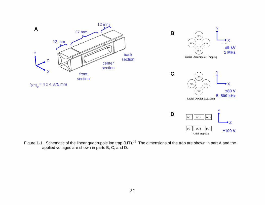
The 2-D trap is constructed of four radially symmetric hyperbolic rods split into
three sections, as shown in Figure 1-1A.36 The end sections are 12 mm in length and
the center section is 37 mm in length with 30 mm 0.25 mm ejection slits in two of the
rods. The two y-axis rods are spaced 8 mm apart, while the two x-axis rods (with the
slits) have an additional 0.75-mm stretch to correct for the field imperfections arising
from the slit, much as the spacing of the endcaps of the 3-D trap was stretched to
correct for the holes in the endcaps.38 Different voltages are applied to the various rod
sections of the trap, as shown in Figure 1-1, parts B, C, and D.36 The primary
alternating current (AC) voltage responsible for trapping is applied with matching
polarity to opposing rods and opposite polarity to adjacent rods, typically ±5 kV at
1 MHz. This voltage, when applied to the hyperbolic rods of the specific geometry,
creates a quadrupolar electric field capable of trapping ions which may be located in az
and qz space according to the solutions given for the general form of the Mathieu
equation38, which are provided in Equations 1-1 & 1-2,
(1-1)
22
0
2
02
16
yxm
eUa
z
26
(1-2)
where az is the dimensionless parameter of stability, e is the charge of an electron, U is
the DC amplitude, m is the mass of ion, x0 = y0 is the radial dimension, Ω is the drive
frequency, qz is the dimensionless parameter of stability, and V is the RF amplitude.
The AC voltages for isolation, excitation and ejection are applied with opposite polarity
to opposing rods in the x-axis, typically ±80 V at 5–500 kHz. If the frequency of this AC
voltage matches (is in resonance with) the oscillatory frequency of a given ion, the
amplitude of its oscillations will increase and the ion is ejected through the radial exit
slits. A broadband AC waveform such as SWIFT39,40 or sum-of-sines41 can be applied
to perform mass isolation of a given packet of ions. After isolation, a relatively small AC
voltage, referred to as resonant excitation or tickle voltage, adds sufficient kinetic
energy to the ions for fragmentation for collision-induced dissociation (CID)
experiments. Increasing this RF voltage (to increase the ion’s qz value) linearly allows
for the mass-selective ejection of ions from low to high mass-to-charge. Ejected ions
exit through both radial slits, and impact onto dual ±15 kV conversion dynodes,
producing secondary charged species (electrons or ions) that are detected by the dual
electron multipliers. The current received on the multipliers is matched by a data
acquisition system to the instance when the aforementioned ion packet was ejected
during the RF ramp, resulting in a mass spectrum.
Orbitrap
The Orbitrap is a relatively new mass analyzer capable of high resolving power
and mass accuracy. Both the geometric and mathematical descriptors of the Orbitrap
can be quite complex; hence, only a rudimentary level of detail will be provided,
22
0
2
02
8
yxm
eVq
z
27
sufficient for the purview of this dissertation. The Orbitrap is based upon an
ion-trapping device first invented by Kingdon in 1922, whose shape and applied electric
fields were modified by Knight in 1981.42 It was Makarov and colleagues who adapted
the Knight-modified Kingdon trap for use as an mass analyzer, first as a stand-alone
instrument with an ESI source43 in 2003, then as the mass analyzer in an LIT-Orbitrap
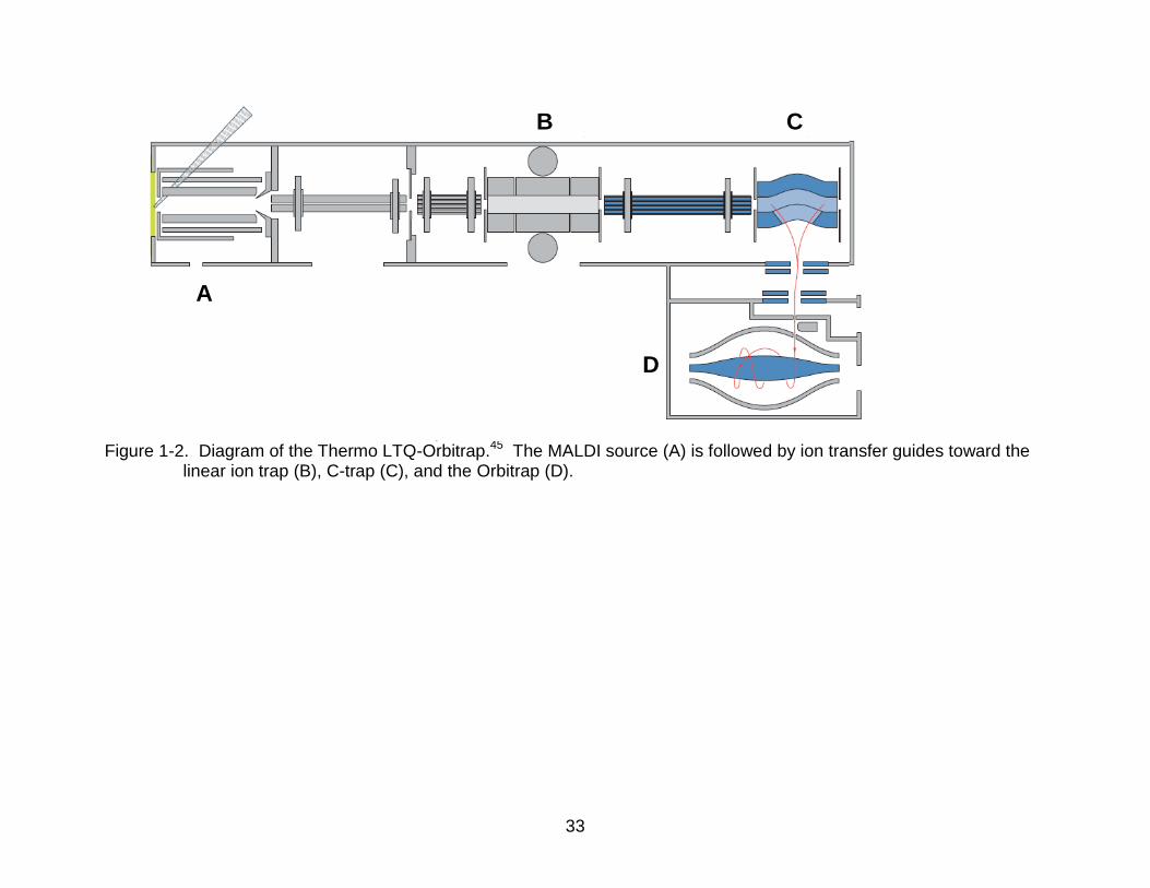
hybrid instrument44 in 2006 (Figure 1-2)45. Because of the Orbitrap’s operational
simplicity, robustness, performance characteristics, and ability to function without a
cryogen or magnet, it has become a principal instrument for proteomics46 and other
applications where high resolution and accurate mass measurements are of paramount
importance.29
The Orbitrap is constructed of a spindle-shaped inner electrode surrounded by a
coaxial barrel-shaped outer electrode, which is split in two halves, and whose inner
surface is nonparallel to that of the spindle, as seen in Figure 1-2D.29 A constant
electrostatic field potential is applied between the two electrodes, which is not constant
across the central axis of the electrodes due to their non-complementary shapes, thus
causing a radial electric field. Following tangential injection, a packet of ions are
effectively “trapped” as they follow a circular (orbital) motion about the spindle electrode
with a radius proportional to the initial kinetic energy of the ion packet from the injection
process and inversely proportional to the electric field from the electrodes, as provided
by Equation 1-3
(1-3)
eE
eVr
2
28
m
zk
where r is the radius of the spindle electrode, eV is the the injected ion packet’s kinetic
energy, and eE is the force of the applied electric field.47 The ion packet is injected via a
specially designed trapping device (C-trap, Figure 1-2C) new to the Orbitrap mass
spectrometer that allows a very narrow pulse of ions from the LIT to be collected and
“cooled down”.48
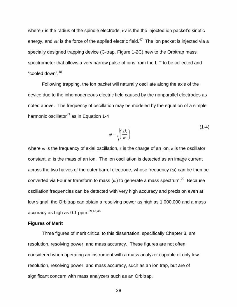
Following trapping, the ion packet will naturally oscillate along the axis of the
device due to the inhomogeneous electric field caused by the nonparallel electrodes as
noted above. The frequency of oscillation may be modeled by the equation of a simple
harmonic oscillator47 as in Equation 1-4
(1-4)
where ω is the frequency of axial oscillation, z is the charge of an ion, k is the oscillator
constant, m is the mass of an ion. The ion oscillation is detected as an image current
across the two halves of the outer barrel electrode, whose frequency (ω) can be then be
converted via Fourier transform to mass (m) to generate a mass spectrum.29 Because
oscillation frequencies can be detected with very high accuracy and precision even at
low signal, the Orbitrap can obtain a resolving power as high as 1,000,000 and a mass
accuracy as high as 0.1 ppm.29,45,46
Figures of Merit
Three figures of merit critical to this dissertation, specifically Chapter 3, are
resolution, resolving power, and mass accuracy. These figures are not often
considered when operating an instrument with a mass analyzer capable of only low
resolution, resolving power, and mass accuracy, such as an ion trap, but are of
significant concern with mass analyzers such as an Orbitrap.
29
12mmm
m
M
mm
MR
12
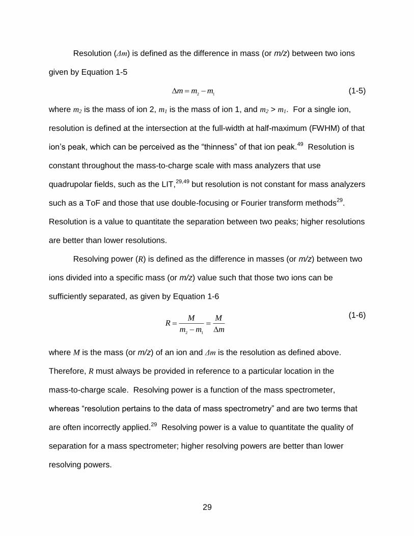
Resolution (Δm) is defined as the difference in mass (or m/z) between two ions
given by Equation 1-5
(1-5)
where m2 is the mass of ion 2, m1 is the mass of ion 1, and m2 > m1. For a single ion,
resolution is defined at the intersection at the full-width at half-maximum (FWHM) of that
ion’s peak, which can be perceived as the “thinness” of that ion peak.49 Resolution is
constant throughout the mass-to-charge scale with mass analyzers that use
quadrupolar fields, such as the LIT,29,49 but resolution is not constant for mass analyzers
such as a ToF and those that use double-focusing or Fourier transform methods29.
Resolution is a value to quantitate the separation between two peaks; higher resolutions
are better than lower resolutions.
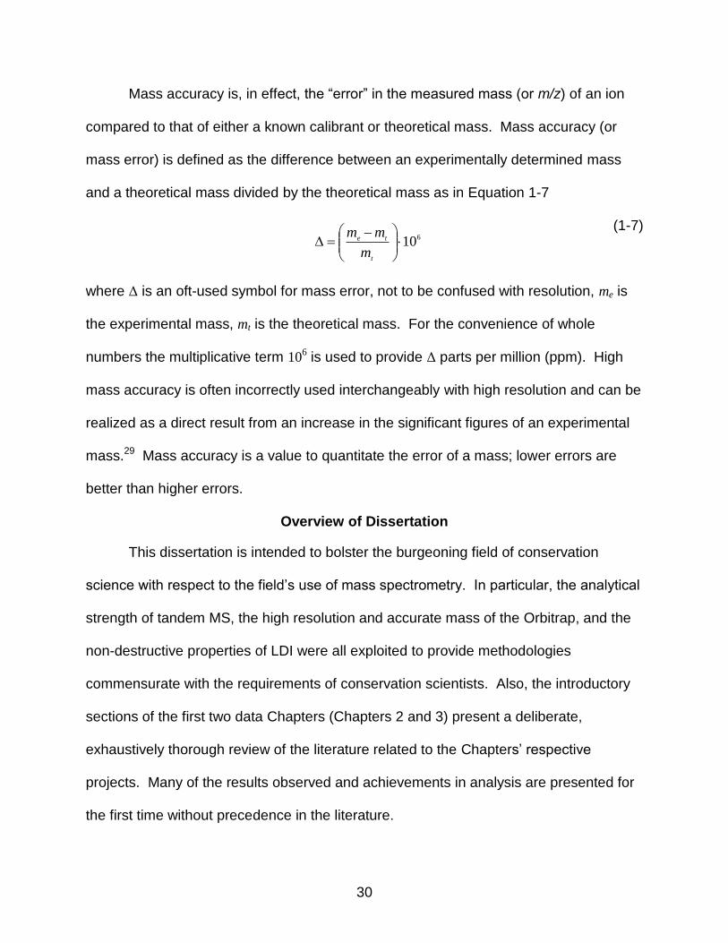
Resolving power (R) is defined as the difference in masses (or m/z) between two
ions divided into a specific mass (or m/z) value such that those two ions can be
sufficiently separated, as given by Equation 1-6
(1-6)
where M is the mass (or m/z) of an ion and Δm is the resolution as defined above.
Therefore, R must always be provided in reference to a particular location in the
mass-to-charge scale. Resolving power is a function of the mass spectrometer,
whereas “resolution pertains to the data of mass spectrometry” and are two terms that
are often incorrectly applied.29 Resolving power is a value to quantitate the quality of
separation for a mass spectrometer; higher resolving powers are better than lower
resolving powers.
30
610
t
te
m
mm
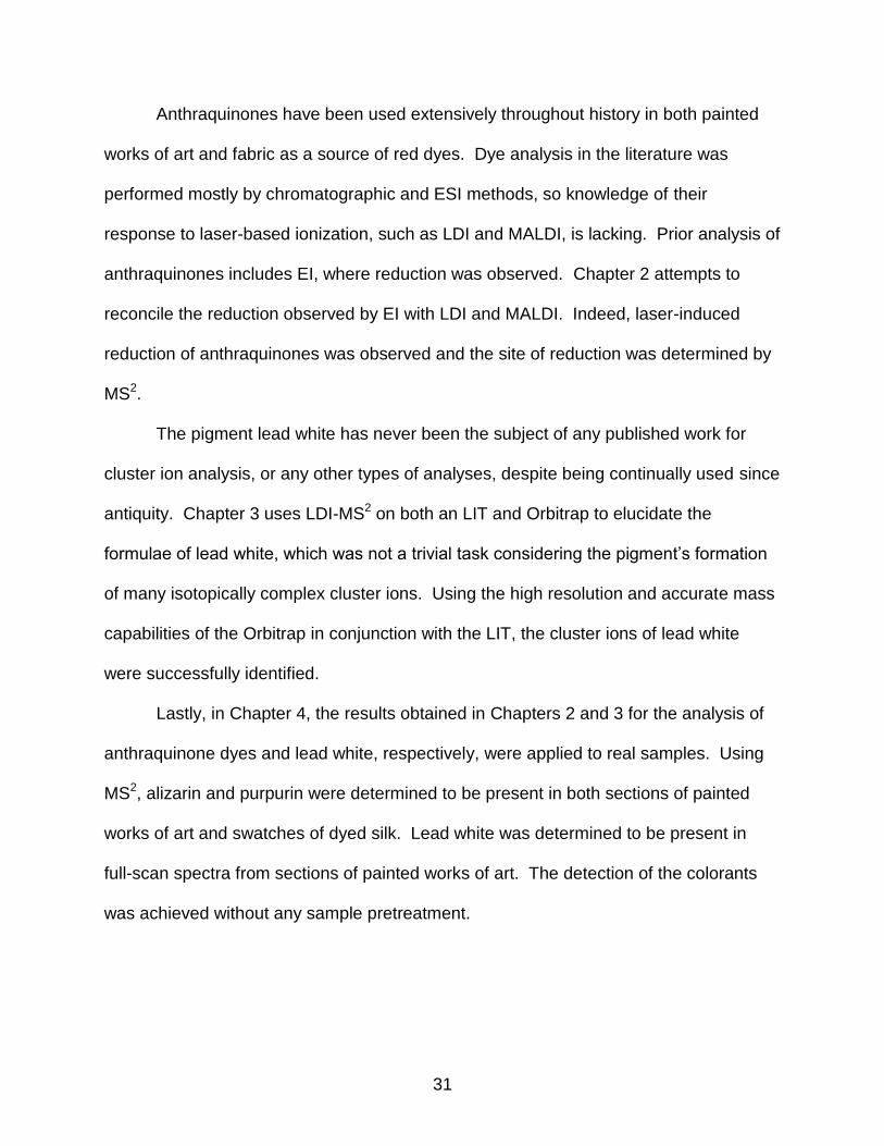
Mass accuracy is, in effect, the “error” in the measured mass (or m/z) of an ion
compared to that of either a known calibrant or theoretical mass. Mass accuracy (or
mass error) is defined as the difference between an experimentally determined mass
and a theoretical mass divided by the theoretical mass as in Equation 1-7
(1-7)
where Δ is an oft-used symbol for mass error, not to be confused with resolution, me is
the experimental mass, mt is the theoretical mass. For the convenience of whole
numbers the multiplicative term 106 is used to provide Δ parts per million (ppm). High
mass accuracy is often incorrectly used interchangeably with high resolution and can be
realized as a direct result from an increase in the significant figures of an experimental
mass.29 Mass accuracy is a value to quantitate the error of a mass; lower errors are
better than higher errors.
Overview of Dissertation
This dissertation is intended to bolster the burgeoning field of conservation
science with respect to the field’s use of mass spectrometry. In particular, the analytical
strength of tandem MS, the high resolution and accurate mass of the Orbitrap, and the
non-destructive properties of LDI were all exploited to provide methodologies
commensurate with the requirements of conservation scientists. Also, the introductory
sections of the first two data Chapters (Chapters 2 and 3) present a deliberate,
exhaustively thorough review of the literature related to the Chapters’ respective
projects. Many of the results observed and achievements in analysis are presented for
the first time without precedence in the literature.
31
Anthraquinones have been used extensively throughout history in both painted
works of art and fabric as a source of red dyes. Dye analysis in the literature was
performed mostly by chromatographic and ESI methods, so knowledge of their
response to laser-based ionization, such as LDI and MALDI, is lacking. Prior analysis of
anthraquinones includes EI, where reduction was observed. Chapter 2 attempts to
reconcile the reduction observed by EI with LDI and MALDI. Indeed, laser-induced
reduction of anthraquinones was observed and the site of reduction was determined by
MS2.
The pigment lead white has never been the subject of any published work for
cluster ion analysis, or any other types of analyses, despite being continually used since
antiquity. Chapter 3 uses LDI-MS2 on both an LIT and Orbitrap to elucidate the
formulae of lead white, which was not a trivial task considering the pigment’s formation
of many isotopically complex cluster ions. Using the high resolution and accurate mass
capabilities of the Orbitrap in conjunction with the LIT, the cluster ions of lead white
were successfully identified.
Lastly, in Chapter 4, the results obtained in Chapters 2 and 3 for the analysis of
anthraquinone dyes and lead white, respectively, were applied to real samples. Using
MS2, alizarin and purpurin were determined to be present in both sections of painted
works of art and swatches of dyed silk. Lead white was determined to be present in
full-scan spectra from sections of painted works of art. The detection of the colorants
was achieved without any sample pretreatment.
32
Figure 1-1. Schematic of the linear quadrupole ion trap (LIT).36 The dimensions of the trap are shown in part A and the
applied voltages are shown in parts B, C, and D.
12 mm
37 mm
12 mm
0 r(X,Y) = 4 x 4.375 mm
±100 V
±5 kV
1 MHz
front section
center section
back section
X
Z
Y
Y
X
Y
X
Y
Z
A B
C
D
±80 V
5–500 kHz
33
Figure 1-2. Diagram of the Thermo LTQ-Orbitrap.45 The MALDI source (A) is followed by ion transfer guides toward the linear ion trap (B), C-trap (C), and the Orbitrap (D).
A
B C
D
34
CHAPTER 2 TANDEM MASS SPECTROMETRY OF ANTHRAQUINONES
Background
The pursuit of improved visual aesthetics is a hallmark of man’s desire for beauty.
That basal desire is manifested in the addition, alteration, and manipulation of color to
common and distinct objects such as garments, décor, and works dedicated as art.
Before the advent of modern chemistry, molecules for coloring were developed from
natural sources. Inorganic, water-insoluble pigments were usually obtained from
minerals, ores, and rudimentary chemical preparation50, while organic, water-soluble
dyes were harvested from animal and plant sources. Organic dyes are classified into
three color groups51,52, which arise (with some exceptions) from different chemical
classes: blue (indigotins), yellow (carotenoids and flavonoids), and red
(anthraquinones), the last of which is the focus of this Chapter. Anthraquinones can be
further sub-classified as either animal, such as lac from the insect Kerria lacca and
cochineal from the insect Dactylopius coccus, or plant, such as madder from the root of
Rubia tinctorum.52,53 Moreover, there are many different isomers and analogues of
dyes from a particular source, and dyes are also found in many genera and species of a
family, as in the case of madder. For instance, madder is the general term for at least
thirty-six different anthraquinone-based red dyes that may be found in at least four
different species of the genus Rubia, which is within the family Rubiaceae.54,55 Because
of such factors as color quality and light fastness, by far the most significant, notable,
and well-studied anthraquinone in madder is alizarin (1,2-dihydroxyanthraquinone), and
to a lesser extent its analogue purpurin (1,2,4-trihydroxyanthraquinone).55,56
35
The use of madder dyes have been known since antiquity, originating first from the
East then west to ancient Persia and Egypt before arriving in ancient Greece and
Rome.57 In fact, madder is the oldest known textile dye, having been found as the dye
of a belt in Tutankhamun’s tomb from 1350 BC.55 Rubia’s importance as the feedstock
for red dye led it to be widely cultivated in Europe until alizarin was first synthesized in
1868, the first chemical synthesis of a natural dye.57,58 Indeed, at the time of alizarin’s
synthesis, up to one-half of a million acres, roughly the area of Luxembourg, was used
in Europe to cultivate the Rubia crop.59 Yet, not all species of the Rubiaceae family
contain alizarin, as is the case of some South American species of the genus
Relbunium, and certainly not all species of the family contain the same relative amount
of anthraquinones.60-62 Indeed, determining the particular species of Rubia from where
madder root extracts were obtain has been a factor in the analyses of madder,
accomplished by HPLC-diode array detection (DAD), HPLC/ESI-MS, and
GC/EI-MS.54,62
Because of the many similarly structured anthraquinones in madder from extracts
of Rubia spp., analyses of madder dyes have understandably used separations such as
HPLC, CE, and GC prior to DAD or MS detection.60,62-65 Because of madder’s history
as a textile dye, many analyses have focused on the detection of anthraquinones
extracted from dyed textiles using GC/EI-MS,66 HPLC/TSP-MS67, HPLC-DAD61, and
HPLC-DAD/ESI-MS54,68-70. When alizarin or purpurin were able to be detected with MS,
in cases not using EI they were observed as the [M+H]+ or [M−H]− ion for positive or
negative mode, respectively. Recently, direct analysis in real time (DART)-MS was
demonstrated to provide rapid analysis of madder on a textile and even directly from
36
madder root.71 Alizarin and purpurin were both detected as [M+H]+ ions. Although
DART may be amenable to the conservation science field because of its
non-destructiveness, DART still suffers from being a relatively esoteric, underutilized
ionization technique that cannot provide the separation of similar molecules with in-line
chromatographic separation. Moreover, the cited DART analysis was conducted on a
TOF instrument incapable of tandem MS. Although DART’s direct detection may be an
improvement compared to the destructiveness of extraction required for HPLC-based
methods, direct detection is still dominated by laser-based ionization sources such as
LDI and MALDI.
The first laser-based ionization mass spectrometric method for the analysis of
artists’ dyes was published in 1990, but was for modern synthetic dyes.72 Then in 1993,
a second article was published on the two-step infrared laser desorption ultraviolet laser
ionization time-of-flight mass spectrometry (L2ToFMS) of natural dyes.73 Although
twelve dyes were analyzed in that work, the one most relevant to this Chapter was
disperse blue 1 (1,4,5,8-tetraaminoanthraquinone) since it is an anthraquinone dye and
was noted to appear as [M]+, [M+Na]+, and [M+2Na]+ ions. In 2003, much highly cited
work was conducted by Donna Grim as a doctoral student in Dr. John Allison’s
laboratory on the LDI-ToFMS, working directly from paper and illuminated
manuscripts.74-76 However, these works primarily deal with inorganic pigments, hence
they will considered in the Chapters 3 and 4 of this dissertation. The first and still one of
the most comprehensive laser-based analyses of both anthraquinones—particularly
alizarin, among other dyes—and direct analysis of painted works of art was the 2003
dissertation of Nicolas Wyplosz as a doctoral student of Jaap Boon.77 Alizarin samples,
37
both neat and from a dyed textile, were analyzed with both LDI and MALDI on a 2-D
QIT, yet no tandem MS was conducted. The displayed LDI spectrum shows alizarin in
the positive ion mode as the [M+H]+ ion at m/z 241. Critically important to the work
present in this Chapter, an ion with very high intensity was shown at m/z 242, which
Wyplosz claimed was the 13C isotope of m/z 241. However, the m/z 242 ion had an
intensity that was ≈95% of the m/z 241 ion even though the theoretical distribution for
the 13C isotope should be 15.4% of an [M+H]+ ion of alizarin, given just 14 carbon atoms
in the molecule. This discrepancy will be thoroughly covered in this Chapter of this
dissertation. In 2007, the MALDI-ToF analysis of dyes and pigments was published in
which the major ions of 58 neat samples were catalogued.78 In this work, alizarin was
detected only in the negative ion mode as the [M−H]− ion at m/z 239. In 2008, the
LDI-ToF analysis of madder standards was published in which alizarin and purpurin
were observed only in the negative ion mode.79 Both molecules were shown in spectra
to appear at mass-to-charge ratios for their respective [M−H]− and [M] •− ions. Lastly, in
2009, work was published on the LDI-ToF analysis of modern pigments and dyes from
standards and samples of painted works of modern art, yet no anthraquinones were
tested.80
Most significant for this Chapter was the work published in 2007 on the
MALDI-ToF analysis of synthesized anthraquinone derivatives.81 The authors, whose
expertise is in synthetic organic chemistry,82 made the remarkable claim that their
anthraquinones underwent never-before-documented “double cationization”, that is, two
protons or sodium ions were adducted, yet the ion remained singly charged. The
peculiar ions observed were [M+2H]+, [M+2Na]+, and [M−H]+. This phenomenon is
38
purportedly caused by the electron-deficient anthraquinones from the dipoles of their
carbonyl groups, although this claim was poorly substantiated by the lack of both direct
evidence and proper citation. Hence, in the hypothesized gas-phase ionization
mechanism, addition of an extra proton occurred concomitantly with the addition of an
electron. The authors justify their claim with the following experimental findings:
1) The electron capture ability (double cationization) of the anthraquinones was significantly increased with the electron-withdrawing capability of the substituents. 2) Negative ion mode shows only negative radical ions, [M] •−.
3) Whether using the thin-layer deposition method or a basic matrix, the phenomenon still was observed. 4) Matrix acidity had no considerable influence.
5) Phenomenon was not observed with ESI+.
Lastly, without support by direct evidence or citation the authors rule out the possibility
of this phenomenon simply stemming from reduction because “anthraquinones have a
very stable conjugated backbone and no bond can be readily reduced.”
Yet, MALDI reduction of analytes has been extensively researched and published
by some notable mass spectrometry groups. The evidence supporting the presence of
electrons generated through the “lucky survivor” model of the MALDI process was
introduced in 2000 by Karas et al.83 Experimental confirmation of free electrons
generated by the MALDI laser occurred in 2002 and 2003 by Zenobi et al. when they
documented the photoelectric effect, from the UV photons interacting with the metal
MALDI sample plate, as the fundamental source of electrons produced.84,85 It was
shown that a decreased number of electrons correlated to the impediment of photons
impinging the sample plate: samples with a thickness >1 mm had negligible production
39
of photoelectrons84, and samples completely separated from the plate with a piece of
adhesive tape experienced a >100-fold increase in positive ions85. With an elegant set
of experiments, Zenobi et al. also definitively proved that laser ionization caused copper
salts to be reduced from Cu(II) to Cu(I) with higher yields at higher laser fluence and
without regard to the presence of matrix, steel substrate, or combination thereof, as
observed in both positive and negative ion modes.86
In 2004, a Japanese group published observations on the MALDI reduction of the
chloride salts of four organic dye cations, which contained fused rings similar to
anthraquinone, although without a quinone moiety.87 The extent of reduction, via
electron transfer and protonation, was shown to increase as a function of both
increased matrix-to-analyte ratio and the analytes’ reduction potential, and decrease
upon addition of Cu(II) as an electron scavenger. Yet, the work tested the dyes only
with MALDI matrix, on a steel sample plate, in positive ion mode, without discussion of
the possible site of protonation, and without CID since a ToF was used.
Lastly, in 2008 a Ukrainian group published comprehensive work on the reduction
of four imidazophenazine dye derivatives, which have four fused nitrogen-containing
rings.88 In the positive ion mode singly and doubly reduced dyes, [M+2H] •+ and
[M+3H]+, respectively, were observed by FAB in glycerol, MALDI, LDI on steel, LDI on
graphite, and low-temperature SIMS. In the negative ion mode singly reduced dyes,
[M] •−, were observed by MALDI, LDI on steel, LDI on graphite, ESI, and low-
temperature SIMS; and doubly reduced dyes, [M+H] −, were observed for only LDI on
graphite. Interestingly, the extent of reduction correlated with the electron affinity of the
dyes in the positive ion mode for FAB in glycerol, LDI on steel, and LDI on graphite; and
40
in the negative ion mode for LDI on graphite and ESI. It should be noted that reduction
is not the only effect laser-based ionization methods may have on an analyte. Recent
observations were published on the laser-induced oxidation of cholesterol, which was
thought to have been caused by hydroxyl radicals from irradiated MALDI matrix,
although no definitive proof was provided.89
Reduction–ionization anomalies of anthraquinones do not occur exclusively from
laser-based methods or as protonated cations. Moreover, it is the central ring of
anthraquinones—indeed the benzoquinone moiety—that appears to be the operative
portion to generate ions of the form M+2. Intriguingly, M+2 ions of p-benzoquinone
were first reported in 1966 in a succinct article by Pike et al. in which radical cations
were produced using an EI source at an elevated temperature (250 °C).90 Pike cleverly
conditioned the source region with D2O and observed M+4 peaks in the resultant mass
spectrum, noting “that water is a probable origin of the hydrogen molecule responsible
for the M+2 [ions]”. The use of D2O was repeated in 1967 by Ukai et al. who also
observed increases of M+2 of benzoquinones as functions of source temperature and
time.91
In 1971, Park et al. reported on the isolation and characterization of a
benzoquinone derivative from fungal cultures.92 As a brief side note in the article, they
commented that [M+2]+ ions, as EI-generated radical cations, had formed if the ion
source “had not recently been baked out”, which gives credence to the claims by Pike
and Ukai regarding the role of water. In a pair of papers, Oliver et al. studied the M+2
ion of naphthoquinones as a function of the source’s temperature and water vapor.93,94
Surprisingly, they found no correlation between the napthoquinones’ extent of formation
41
of M+2 and their aqueous redox potential. Furthermore, Taylor et al. published in 1974
comprehensive experiments to explore the M+2 phenomenon—in particular, the effect
of water—using derivatives of polyporic acid, which are centered on benzoquinone.95
They concluded that the abundance of M+2 EI-generated radical cations was
dependent on the 1) temperature of the sample, 2) pressure in the source, and 3) partial
pressure of water in the instrument. In a repeat of Pike’s experiment, when D2O was
added in the source, M+4 ions were also observed. Taylor concluded that the M+2
phenomenon “requires the reduction of…benzoquinone”. Lastly, four more instances of
M+2 EI-generated radical cations were reported following the characterization of
benzoquinone and its derivatives from various sources96-99.
Following the exhaustive literature review and background above, it is clear that
ionization of quinone-containing molecules—particularly anthraquinone-based dyes—
can form anomalous M+2 ions, yet the exact process is still not definite. It is of
surprising and significant relevance to note that there exist many articles that use either
an EI or a laser source to ionize quinone- and anthraquinone-containing dyes and other
molecules in which M+2 ions are not observed. Unfortunately, scant experimental
details—particularly from works of the 1960s and 1970s that use EI on sector
instruments—preclude critical analyses that might have revealed a trend to explain this
discrepancy. Although work over twenty years ago has shown interesting results
regarding EI, it is laser-based methods’ ability to incite atypical ionization of analytes,
particularly dyes, that is most applicable to the contemporary, growing field of
conservation science.
42
Considering that in all of the aforementioned laser-based publications known
molecules were analyzed, it begets the question on how the ionization phenomena
would complicate the elucidation of unknown analytes or molecules forming ions with
isobaric mass-to-charge ratios. Moreover, none of the publications with laser-based
methods were able to perform tandem mass spectrometry, which might have revealed
sites of reduction, glimpses on mechanisms, or isobaric interferences. With the
exception of the seminal work by Pike, all of the publications with EI-based methods did
provide EI-generated fragmentation. Yet, the fragmentations, which will be discussed
later, were not able to provide conclusive evidence of the cause or site of the M+2
phenomenon. Certainly, the need for MS/MS is apparent and fulfilled herein.
Experimental Methods
Chemicals and Materials
Formic acid (FA) and MALDI matrix 2,5-dihydroxybenzoic acid (DHB), were
purchased from Acros Organics (Morris Plains, NJ). Whatman filter paper, acetonitrile
(ACN), HPLC-grade methanol (MeOH), tetrahydrofuran (THF), and water were
purchased from Fisher Scientific (Fairlawn, NJ). Anthraquinone standards of varying
purity (anthraquinone, 99.5%; 1,2-dihydroxyanthraquinone (alizarin), 85%;
1,2,4-trihydroxy-anthraquinone (purpurin), 90%; 1,5-dihyrdroxyanthraquinone, 85%;
2,6-dihydroxyanthraquinone, 90%; 1,5-diaminoanthraquinone, 85%; and
2,6-diaminoanthraquinone, 97%) were purchased from Sigma Aldrich (St. Louis, MO)
(Figure 2-1).
Recrystallization of Standards
The standards of both anthraquinone and 1,2-dihydroxyanthraquinone were first
recrystallized using established techniques.100 Although there were slight variations in
43
recrystallization parameters such as total solvent volume, required time for dissolution,
and required time for recrystallization, a generalized workflow for the recrystallization
procedure follows:
1) heat 50 mL of MeOH to boiling
2) transfer 0.5 g of unpurified anthraquinone standard to a clean 50-mL Erlenmeyer flask
3) dispense hot MeOH in a slow, dropwise manner
4) stop addition of hot MeOH immediately following full dissolution of standard
5) cover the saturated solution and store in a cool, dark place
6) filter crystals following overnight recrystallization using filter paper and gravity filtration
7) rise filtered crystals with only a few drops of cold MeOH
8) transfer crystals to a watch glass to allow drying
The recrystallized anthraquinones were stored in darkened vials until use to prevent
exposure to ambient light.
Preparation of Chemicals
All recrystallized anthraquinone standards were first dissolved at a concentration
of 1000 ppm in THF. Initial dissolution in THF was a necessary step due to the limited
solubility of most of the anthraquinones in a mobile phase suitable for electrospray.
Furthermore, THF was selected as the initial solvent since it possesses the necessary
lower hydrophobicity to dissolve the anthraquinones, yet is still itself fully soluble in
water. Thereafter, stock solutions were serially diluted in 50/50 ACN/H2O to
concentrations of 100 ppm, 10 ppm, and 1 ppm and stored in a dark drawer at room
temperature until use. For preparation of electrospray mobile phase, 0.1% FA was
44
added. The MALDI matrix DHB was prepared at a concentration of 40 mg/mL in 70/30
MeOH/H2O and stored in a freezer until use.
Electrospray Ionization Parameters
As a set of control experiments that ionize anthraquinones without the use of light
(i.e., laser-generated UV photons), electrospray ionization mass spectrometry was
used. A Finnigan LCQ (San Jose, CA) was used with its standard electrospray source.
All solutions (10 ppm) were directly infused at a flow rate of 10 μL/min. The applied
potential on the ESI needle was +4.00 kV. The heated capillary was kept at 200.0 °C
and at +40.0 V. All other ESI and ion optics parameters such as auxiliary and sheath
gas flow rates, tube lens voltage, and lens and multipole offsets, were separately tuned
for each standard analyzed. All spectra were recorded with automatic gain control
(AGC) enabled for the target value of a normalized signal of 7.0 107 and with three
microscans averaged per recorded analytical scan.
All of the aforementioned parameters for recording a full scan were kept constant
for tandem mass spectrometry. Additionally, the isolation width for all MS/MS spectra
was adjusted to isolate only one profile peak in an isotopic envelope of a given analyte,
which is critical for the experiments in this Chapter. As shown in Figure 2-2, the
optimized value for isolation width was determined to be a 0.8-Da window, which was
based upon the balance between a) obtaining maximal daughter ion intensities and b)
preventing truncation of the peak of the desired parent ion while omitting undesired,
interferent neighboring parent ions. Collision-induced dissociation (CID) parameters
were optimized using manual tuning. The parent mass was first isolated and the CID
energy was increased in increments of 0.5 (arbitrary units) from 20 to 50. Optimized
45
CID values were declared for the observed CID interval at which the signal intensity of
the parent ion dropped to 10% of the sum of intensities for the parent ion and the two
most abundant daughter ions. A representative plot of this CID determination is shown
in Figure 2-3, which would yield an optimized CID energy of 38. The average value for
CID energies was 41 among all tested anthraquinones.
Laser Desorption/Ionization and Matrix-Assisted Laser Desorption/Ionization Parameters
All LDI and MADLI experiments were performed on a Thermo Finnigan LTQ-XL
(San Jose, CA) equipped with an intermediate-pressure (≈170 mTorr) MALDI source
and a N2 laser ( = 337 nm). Standard solutions of anthraquinones were spotted with a
volume of 1 μL on a polished stainless steel MALDI-sample plate or glass microscope
slides. For LDI experiments, the deposited solutions were allowed to dry unaided at
ambient conditions before being inserted and analyzed in the instrument.
For MALDI experiments, a modified dried-droplet method was employed.101 The
dried-droplet method as indicated in the literature has a separate vial that is used to
pre-mix the analyte and matrix solutions before that newly mixed solution is spotted on
a sample plate. The modified dried-droplet method that was employed for this work
avoids the use of a separate vial since the analyte solution (1 μL) and matrix solution
(1 μL) are consecutively and quickly deposited directly on a sample plate. Thereafter,
the deposited solution was allowed to dry unaided at ambient conditions before being
inserted and analyzed in the instrument.
Instrumental parameters such as the front lens voltage were automatically tuned to
maximize the abundance of the base peak, which, in the case of MALDI spectra was
unavoidably the DHB ion at m/z 154. Laser parameters were manually tuned to obtain
46
maximal signal for the ion of interest, yet minimizing the consequent increase in both
baseline and space-charge effects. Typical laser energies were approximately
10 μJ/pulse for LDI and 5.0 μJ/pulse for MALDI. The desired ionization metric of laser
fluence can only be estimated at 1.3 103 J/m2 for LDI and 6.4 102 J/m2 for MALDI due
to the difficulty in an accurate and precise measurement of the laser spot size, which
has an approximate 100-μm spot. The number of laser pulses for each analytical scan
was controlled by the automatic gain control (AGC) to maximize the total ion signal, yet
not exceed the target value of 3.0 104. Most often, the AGC-determined number of
laser pulses was nine. When samples were spotted on a stainless steel MALDI sample
plate with dedicated sample wells, the plate was moved with respect to the stationary
laser in either a “spiral outward” motion or automatically controlled via the software’s
“crystal positioning system”. Considering that samples spotted on glass slides did not
have dedicated sample wells that were recognized by the software, the sample holder
was moved in a raster pattern within a user-defined area via the software’s “imaging”
mode.
All of the aforementioned parameters for recording a full scan were kept constant
for tandem mass spectrometry. The isolation width for all MS/MS spectra was adjusted
to isolate only one profile peak in an isotopic envelope of a given analyte. The
optimized value for isolation width was determined to be a 0.8-Da window. CID
parameters were optimized using the software’s automatic tuning. The parent mass
was isolated and the CID energy was increased in increments of 0.5 (normalized
instrumental values) from 20 to 50. Optimum CID values were defined as the point at
which the parent ion intensity was reduced to 10% of the most intense peak in the
47
daughter-ion spectrum. Typical values for CID energies were approximately 30 for all
tested anthraquinones.
Ultraviolet–visible (UV) Light Exposure
To explore the model of photoreduction, anthraquinone was exposed to UV light
for an hour and its UV–vis spectrum was then recorded. A freshly prepared 10-ppm
solution of anthraquinone was prepared via dilution according to the method above.
The control aliquot was dispensed in to a quartz cuvette and placed in a dark drawer
until analyzed. The test aliquot was dispensed in to a quartz cuvette and placed in a
custom-made chamber (≈30 cm lwh) constructed from black poster board. The
cuvette was placed ≈15 cm from a UVP, Inc. UVG-11 (San Gabriel, CA) 4-W ultraviolet
TLC lamp ( = 254 nm) for 1 h. Thereafter, both cuvettes were analyzed in a
Hewlett-Packard 8450A UV–vis spectrophotometer (Paolo Alto, CA).
Results and Discussion
Upon preliminary analyses for the mass spectrometric imaging of the dyes known
to be present in the obtained painting cross sections, data revealed the peculiar—and
initially quite perplexing—ionization of alizarin. Both laser desorption/ionization and
matrix-assisted laser desorption/ionization analyses of alizarin standards had shown a
base peak whose identity was not readily understood, even after preliminary tandem
mass spectrometric analysis. An initial review of the literature generated the recently
published and seemingly promising article by Meijer et al.81, which suggested
anthraquinones ionize via “‘double cationization”—a manner counter to all previously
published mass spectral data. This phenomenon and how it may affect conservation
scientists’ interpretation of mass spectral data of anthraquinone dyes, such as alizarin,
48
brought the further and thorough tandem mass spectrometric investigations described
herein.
As will be henceforth detailed, alizarin and similar anthraquinones undergo
peculiar ionization via reduction (but not double cationization), which is supported by
both the thorough literature review in the introduction of this Chapter and the following
experimental evidence, as discussed later in this Chapter:
1) LDI and MALDI cause reduction of anthraquinones, which is observed as an ion in the form [M+2H] •+.
2) ESI does not cause appreciable reduction of anthraquinones despite the
aqueous, acidic mobile phase. 3) The site of reduction is the anthraquinones’ carbonyl oxygen, which was
elucidated by tandem mass spectrometry. 4) Anthraquinone undergoes photoreduction at ambient conditions, which was
confirmed by ESI-MS/MS. 5) The extent of reduction for alizarin and anthraquinone increases as a function
of analyte concentration with both LDI and MALDI. 6) The extent of reduction for alizarin and anthraquinone decreases as a function
of matrix-to-analyte ratio with MALDI.
Electrospray Ionization of Anthraquinones
Electrospray ionization was used, in effect, as the control ionization method. With
the lack of UV photons, ESI may provide confirmation of the null hypothesis, which
states that the ionization phenomenon, specifically the formation of [M+2H] •+ ions, of
anthraquinones would not be possible without the presence of UV photons. Naturally,
the fundamental difference between ESI and both LDI and MALDI regarding factors
such as causal mechanisms of ionization (i.e., without or with UV photons), phase (i.e.,
aqueous or solid), and source pressure (i.e., ambient or low vacuum), precluded any
variable control among the two classes of ionization methods. Also, all ESI experiments
49
were performed on an LCQ, which is a three-dimensional quadrupole ion trap, whereas
all LDI and MALDI experiments were performed on an LTQ, which is a two-dimensional
quadrupole ion trap. Despite the geometric differences between the 3-D and 2-D traps
and all the associated ion optics and requisite voltages applied therein, the two versions
of the QIT played no discernable part in experimental variability. That is, experiments
were designed as such to only observe changes in ionization after altering the ionization
variable. When performing tandem mass spectrometry, there is a slight difference in
some instrumental parameters for MS/MS. The internal kinetic energy of the analytes
as imparted by the CID energy, which is a normalized value set by the manufacturer,
may vary between the LCQ and the LTQ. Therefore, all daughter-ion spectra will
slightly vary depending on the instrument used. Nevertheless, the respective
daughter-ion spectra are still amenable for comparison since differences in the CID
among the two instruments would have only differences in imparted—not delivery
modes of—kinetic energy and would simply be observed as providing slightly varying
intensities of daughter ions—and not differences in actual fragmentation pathways and
consequent daughter ions. Lastly, the amount of internal energy imparted into the ions
during ionization will vary among the three methods (i.e., LDI, MALDI, and ESI).
As observed in Figure 2-4A, the positive mode ESI spectrum of
1,2-dihydroxyanthraquinone (alizarin, MW = 240) produced a singly protonated,
non-reduced ion at m/z 241, [M+H]+. Of course, this is the ion one would expect from
alizarin and shall be henceforth referred to as “P” (parent), which is a nomenclature
historically used, albeit increasingly infrequent, by mass spectrometrists. The ion at
m/z 242 shall be henceforth referred to as “P+1” (parent+1 Da) and incorporates the 13C
50
isotope contribution of P. The experimental P+1 peak has an intensity of 20.6, which is
normalized to the experimental P peak, and is marginally higher than the normalized
P+1 peak (15.4) for the theoretical spectrum of a 14-carbon compound. The reason for
the higher experimental P+1 peak for anthraquinone, and some of the other compounds
tested, may be a result of spectral interference that may arise from both impurity of the
standard and limited ESI-induced electrochemical reduction102. The ion at m/z 243 shall
be henceforth referred to as P+2 (parent+2 Da) and incorporates both the 18O isotope
contribution of P and the 13C contribution of P+1. The experimental P+2 peak has an
intensity of 2.72, which is normalized to the experimental P peak, and is quite close to
the normalized P+2 peak (1.93) for the theoretical spectrum given two oxygens.
Considering that the ESI mobile phase was 50% water, the role of water in the
production of M+2 ions, as was observed with prior experiments cited in the
introduction, is questionable and inconclusive.90,92,95 These three ion peaks are all
predicted by the spectrum of theoretical isotopic distribution for alizarin, which is shown
in Figure 2-4B as an overlay on the experimental spectrum. The two spectral plots
closely overlap since they share peaks with similar abundances at the same m/z, yet
there is a slight shift of the experimental spectrum to a higher m/z. This shift might be
explained by the possibilities of both small space charging and unoptimized calibration.
For instance, the lowest-mass calibrant used for the LTQ is the peptide MRFA, which
has an [M+H]+ ion at the monoisotopic m/z of 524.27—close to double the m/z of the
tested anthraquinones.
Alizarin was discussed as the exemplar case. Indeed, for all of the compounds
tested, the ESI-generated experimental and theoretical spectra overlap, as shown in
51
parts A and B in Figures 2-4, 2-6, 2-8, 2-10, 2-12, 2-14, 2-16. The tabulated summary
of theoretical and experimental spectra for all anthraquinones tested appears in Table
2-1. The reason for the higher experimental P+1 peak for anthraquinone;
1,2-dihydroxyanthraquinone; 1,5-dihydroxyanthraquinone; and
2,6-dihydroxyanthraquinone may be a result of spectral interference that may arise from
impurity of the standard and limited ESI-induced electrochemical reduction102.
Although, there was no apparent correlation observed between a higher P+1 peak and
purity of the standards.
Tandem mass spectrometry was performed on both the P and P+1 peaks for all
anthraquinones tested. Again, alizarin will be treated as the exemplar case. As shown
in Figure 2-5, parts A and B, the daughter ion spectrum of m/z 241, P, closely
corresponds to the daughter ion spectrum of m/z 242, P+1. Although the m/z values of
the daughter ions differ by 1 Da, the neutral loss (NL) values, which indicate the
fragmentation of the parent ion, are the same. The NL of 28 is derived from the loss of
CO from one carbonyl functional group about the central quinone backbone that forms
the fluorenone ion, which is supported by numerous articles, albeit by the fragmentation
of EI-generated, odd-electron, radical cations.66,95,97,103-108 Furthermore, as Beynon et
al. proved with 18O-labeled 1-hydroxyanthraquinone, the loss of 28 is highly favorable as
the loss of carbon monoxide from the carbonyl rather than the hydroxyl portion.107 The
loss of 28 is seen with high abundance in all anthraquinones except the two
diaminoanthraquinone compounds (Figures 2-13 and 2-15, parts A and B). Those two
amino compounds preferentially fragment with a cross-ring cleavage, observed as a NL
of 93, which incorporates carbon positions 1, 2, 3, 9, and 13 (or 5, 6, 7, 10, and 11) and
52
respective substituents. Interestingly, when the same two amino compounds were
analyzed in 1960 by Beynon et al. as EI-generated odd-electron, radical cations, a
similar cross-ring cleavage was not observed, but the loss of carbon monoxide was103;
however, Bowie et al. did observe cross-ring cleavage for derivatives of
benzoquinones.104
The NL of 46 is observed in ESI spectra only for alizarin. This loss is attributed to
the loss of one carbonyl functional group and one water. Although this loss, which may
be realized by the possible interaction of the carbonyl and the hydroxy at the 9 and 1
positions, respectively, has a significant role in the fragmentation pathway of
anthraquinones reduced via LDI or MALDI, its appearance is not completely understood
at this time. Also, the other two compounds that might experience a similar interaction
with a hydroxy at the 1 position (1,2,4-trihydroxyanthraquinone, Figure 2-7 A and B, and
1,5-dihyroxyanthraquinone, Figure 2-9 A and B) do not exhibit a loss of 46.
The NL of 56 is derived from the loss of two CO moieties from two carbonyl
functional groups to form an ion of biphenylene. This consecutive loss has been well
documented, albeit for EI-generated odd-electron, radical cations.66,97,103-108 The three
compounds that exhibit cross-ring cleavage thereby losing one carbonyl [1,5- and
2,6-diaminoanthraquinone (Figures 2-9 and 2-11, parts A and B) and
1,2,4-trihydroxyanthraquinone (Figures 2-7 A and B), the latter with cleavage that
incorporates carbon positions 1, 9, and 13 with respective substituents] have the
daughter ion for NL 56 at a relative abundance of less than one percent.
Other losses with relative abundances of note are some cross-ring cleavages,
which ultimately are inconsequential for the aim of this Chapter. For alizarin, the NL of
53
84 suggests a cross-ring cleavage, although the positions about which the cleavage
takes place is unknown (Figure 2-5 A and B). For purpurin, the NL of 42 must be the
loss of carbons 2 and 3 with the attached hydroxyl group (Figure 2-7 A and B).
Interesting bifurcations are observed with the four symmetrical molecules 1,5- and
2,6-dihydroxy (Figures 2-9 and 2-11, parts A and B); and 1,5- and
2,6-diaminoanthraquinone (Figures 2-13 and 2-15, parts A and B) at neutral losses of
120 and 119, respectively. Obviously, the split may occur indistinguishably across
either positions 9–13 and 10–11, or 9–12 and 10–14.
A serendipitous accident allowed for the reduction of anthraquinone to occur under
ambient conditions and be detected with ESI. A volumetric flask containing a 10-ppm
solution of anthraquinone was unintentionally left on a lab bench for the weekend.
Thereafter, an aliquot was used for analysis by ESI, following the addition of 0.1% FA
similar to the normal samples. The resultant spectrum is in Figure 2-18A and shows a
significant P+1-to-P ratio of 2.61, which is much larger than the control’s ratio of 0.223.
In fact, the ambient reduction of anthraquinone has a reduction extent greater than the
1.95 ratio for the LDI-generated spectrum. To confirm that the ion at m/z 210 was
indeed the [M+2H] •+ ion of anthraquinone, tandem mass spectrometry was performed.
As seen in Figure 2-18B, the daughter ion spectrum from m/z 210 clearly shows a
relatively abundant NL of 29 that is assigned as one reduced carbonyl. The reduction of
anthraquinone at ambient and other conditions—especially in an aqueous medium—is a
well-established feature and has been studied spectroscopically for many years.51,59,109-
114 To further explore light-induced reduction, an aliquot from a freshly prepared
10-ppm solution of anthraquinone was irradiated with a UV lamp for 1 h and analyzed
54
by a UV–vis spectrophotometer. When compared to an aliquot of the same solution
that was not exposed to the UV lamp, a hyperchromic (higher) shift of the relatively low
shoulder at 400 nm is apparent, as seen in Figure 2-19A and B. This spectrographic
change in the absorbance of anthraquinone can be reasonably attributed to the
UV-induced reduction phenomenon observed with LDI and MALDI. However, it must be
mentioned that any direct correlation of the two observations warrant caution since the
correlation of molecular structure to UV–vis spectra is ultimately impossible.51 The
UV-irradiated sample was not analyzed with ESI mass spectrometry.
Laser Desorption/Ionization of Anthraquinones
Again using alizarin as the exemplar case, its positive mode LDI spectrum is
shown in Figure 2-4C. What is immediately apparent in this portion of the full spectrum
is that the base peak is not the [M+H]+ ion at m/z 241 (P), but rather, the [M+2H] •+ ion at
m/z 242 (P+1). In fact, as shown in Table 2-1, P+1 is 77% greater than P. Indeed, P+1
is the reduced form of the alizarin ion. Although P is not the dominant ion, it is still
relatively abundant—P is 33.6% of the total ion abundance of the P, P+1, P+2 envelope
(Table 2-2)—and its presence may be explained by the lack of total conversion because
of a limited number of available protons, which will be supported in the following section
on MALDI. The ion at m/z 240 is also present at a very low abundance, which is
undoubtedly the unprotonated radical cation [M] •+. Interestingly, relatively dominant
unprotonated radical cations were observed for 1,2,4-trihydroxy (Figure 2-6C);
1,5-dihydoxy (Figure 2-8C); 2,6-diamino (Figure 2-14C); and 1,5-diaminoanthraquinone
(Figure 2-12C), the last of which has that ion at significantly higher abundance—28.1%
of the P−1 (i.e., radical), P, P+1, P+2 envelope. No discernable trend that correlates the
55
abundance of the radical cations to either structure or functional groups is apparent. It
is important to note that abundance of the P+1 ion peak is produced not solely from the
reduced ion; rather it includes the 1.1% 13C isotope contribution from P. For the
diamino isomers, P+1 also includes the 0.37% 15N isotope from P. Moreover, the
abundance of the P+2 ion peak is a combination of both the 13C and the 0.20% 18O
isotopes contribution of P+1 and P, respectively. The LDI-generated experimental and
theoretical-overlay spectra for all the anthraquinones tested are shown in parts C and D
in Figures 2-4, 2-6, 2-8, 2-10, 2-12, 2-14, 2-16. The tabulated summary of theoretical
and experimental spectra for all anthraquinones is in Table 2-1.
Tandem mass spectrometry was performed on both the P and P+1 peaks for all
anthraquinones tested. The daughter ion spectrum for alizarin, again as the exemplar
case, is shown in Figure 2-5 parts C and D. In Figure 2-5C, the MS/MS spectrum of the
unreduced [M+H]+ ion at m/z 241, P, precisely corresponds to both the P and P+1
daughter ion spectra of the unreduced alizarin ions produced by ESI, as shown in
Figures 2-5A and B. As expected, the neutral losses of the daughter ion mass spectra
of P for all LDI-generated ions of the anthraquinones tested correspond to the neutral
losses of the daughter ion mass spectra of both P and P+1 for all the ESI-generated
ions (Parts A, B, C for Figures 2-5, 2-7, 2-9, 2-11, 2-13, 2-17). The only exception is the
daughter ion at m/z 195 for 2,6-diaminoanthraquinone (Figure 2-15C) that stems from a
neutral loss of 44 Da, which suggests fragmentation to lose CO2; however, this loss is
not seen in any other anthraquinone except as a very low abundant daughter ion for
1,5-diaminoanthraquinone (Figure 2-13C). It follows that the most likely assignment for
the loss that includes nitrogen is one carbonyl and one of the amine groups (i.e.,
56
•CONH2), although the exact structure is neither known nor crucial. This loss seems to
be a violation of the nitrogen rule, which maintains proper parity, but is actually a
commonly observed neutral loss, albeit as a radical. Nevertheless, the appearance of a
relatively abundant NL of 44 from the P ion for 2,6-diaminoanthraquinone in the LDI—
but not the ESI—generated tandem mass spectrum is perplexing.
The heart of these experiments is to elucidate the anomalous P+1 ions, which,
with the following comparison of daughter ions from P+1 to P, will be explained by
model of reduction of one of the carbonyls. Briefly, two critical observations are made
to support the model: 1) reduction of carbonyl produces a decrease in relative
abundance of NLs of 28 and 56, which are losses of CO from one and two carbonyls,
respectively, with the concomitant increase in relative abundance of NL of 29 (HCO•),
which is from one reduced carbonyl (C-O-H); 2) reduction of the carbonyl adjacent to a
substituent at the 1 position causes intramolecular hydrogen bonding and proton
transfer that produces a significant increase in the relative abundance of NLs of 18
(water) or 17 (ammonia) for hydroxyl or amino groups, respectively.
The simplest case to support the first critical observation on the reduction model is
the LDI-generated daughter ion spectrum of reduced anthraquinone, P+1 (Figure
2-17D). It is quite clear that the relative abundance of the daughter ion from the loss of
CO from one carbonyl (NL 28) has drastically decreased while the daughter ion from the
loss of HCO• from one reduced carbonyl (NL 29) is now present. The reason why the
abundance of NL 28 is 40% of the abundance of NL 29 must be due to differences in
the energetics and, perhaps, the kinetics of the two fragmentations. For anthraquinone,
the two carbonyls are indistinguishable, so it would be safe to assume an equimolar
57
reduction of either carbonyl (in a 1:1 ratio). Therefore, the observed 5:2 ratio of the two
daughter ions must be explained by the fragmentation, which stems from the loss of an
odd-electron neutral fragment (HCO•), from the odd-electron parent ion, being more
likely to occur than the loss of an even-electron neutral molecule (CO). Dramatic
decreases in the NL of 28 from P to P+1 can be seen for all other anthraquinones tested
(parts C and D, Figures 2-5, 2-7, 2-9, 2-11, 2-13, 2-15). For the two compounds that do
not exhibit intramolecular hydrogen bonding with a reduced carbonyl (2,6-hydroxy and
2,6-diaminoanthraquinone) similar appearances of NL 29 are seen, also with ratios that
are explained by differences in the energetics of fragmentations (Part D in Figures 2-11
and 2-15). Also, it should be noted that 2,6-diaminoanthraquinone shows a NL of 29—
and not the NL of 28—as a daughter ion from the unreduced form, P (Figure 2-15C).
When judged by itself, the NL of 29 may have been attributed to HCO• from a reduced
carbonyl. Yet, considering the peculiar NL of 44 for this compound noted above it is
apparent that 2,6-diaminoanthraquinone exhibits fragmentation not observed with the
1,5 isomer; therefore, the NL of 29 for P of 2,6-diaminoanthraquinone should be
attributed as loss of CNH3. This NL will nonetheless not violate the reduction model for
this compound, which will be expounded below.
To support the second critical observation on the reduction model, the
LDI-generated daughter ion spectra of the reduced (P+1) isomers of
dihydroxy-anthraquinone must first be compared (Part D in Figures 2-9 and 2-11). The
2,6 isomer has the hydroxyl groups distal to the carbonyl groups at positions 9 and 10;
therefore, no intramolecular hydrogen bonding can occur between a reduced carbonyl
and a hydroxyl group. Observing the daughter ion spectrum from P to P+1, the relative
58
abundance of NL 18 from the loss of water is dramatically decreased and the NL of 17
from the loss of •OH is now present (Figure 2-11C and D). Considering the NL of 17
was not observed from P, this loss might have been erroneously assigned to the OH of
the reduced carbonyl. However, because of the lack of intramolecular hydrogen
bonding, which will soon be described as allowing the hydroxyl group to be lost as
stabilized water, the OH is allowed to be lost on its own. Furthermore, the NL of 45 is
the losses of CO and •OH from both the unreduced carbonyl and a hydroxyl group,
while the NL of 46 is the simultaneous losses from both the reduced carbonyl and a
hydroxyl group. The NL of 46 can also stem from losses of both water and HCO•; yet,
this additional contributing loss would only cause an increase in its abundance relative
to the other important daughter ions (i.e., NLs of 17, 18, 28, 29, 45) and not the
observed decrease. Why the relative abundance of NL 46 is lower than the other
important daughter ions is immediately not clear, except for the possibility of it simply
being a reflection of the difference in energetics arising from the different losses.
The 1,5 isomer of dihydroxyanthraquinone has hydroxyl groups proximal to the
carbonyl groups at positions 9 and 10; therefore, both intramolecular hydrogen bonding
and proton transfer can occur, the latter of which can result in the reduced carbonyl’s
hydrogen transferring to a hydroxyl group that leads to the highly favorable neutral loss
of water. Intramolecular hydrogen bonding in substituted anthraquinones is a well
established feature, particularly in acidic, aqueous media, which has been extensively
studied by spectroscopic methods for many years.51,59,108,109,115,116 As seen in Figure
2-9D, proton transfer leads to a significant daughter ion (m/z 224) with NL of 18 that
dwarfs all other important ions in the spectrum. Since 18O isotopic labeling was not
59
employed for these experiments, it is difficult to differentiate between the loss of water
from the carbon at the 1 (hydroxyl) or 9 (reduced carbonyl) position. MS3 was
performed on the m/z 242 daughter ion (data not shown), generating granddaughter
ions at neutral losses 28 (base peak, bp), 17 (7.0% of bp), and 56 (11% of bp). Since
the NL of 56, which is attributed to the loss of two CO, was seen from the daughter ion,
it is reasonable to assume that the neutral loss of water occurred with the oxygen at the
1 position. Also, there is a still a very low-abundant daughter ion at m/z 214 that is a NL
of 28 (CO), which, at 2.02% of m/z 224, may erroneously be the remnant of the 13C
contribution from P. Yet, a contribution from P is not supported since NL of 46 is seen
as an abundant daughter ion in the reduced form, P+1, of purpurin (Figure 2-7D) and
alizarin (Figure 2-5D), which both have a daughter ion from the NL of 28 from one
unreduced carbonyl. Therefore, by proxy of the presence of a NL of 28 in purpurin and
alizarin, it is reasonable to infer that the NL of 28 in 1,5-dihydroxyanthraquinone is also
from one unreduced carbonyl and, subsequently, the NL of 46 is the combination of
losses of both water and one unreduced carbonyl. Also, along with the very abundant
loss of water, the absence of the loss of a reduced carbonyl (NL 29) for
1,5-dihyrdoxyanthraquinone reinforces the prominence of proton transfer from a
hydroxyl group proximal to the reduced carbonyl and it also suggests proton transfer of
all the reduced carbonyls. Lastly, the bifurcation seen both from P of the 1,5 and 2,6
isomers of dihydroxyanthraquinone and P+1 of the 2,6 isomer is not seen from P+1 of
the 1,5 isomer, which may be attributed to the increased stability given by
intramolecular hydrogen bonds.
60
The daughter ion spectra for both isomers of diaminoanthraquinone (Parts C and
D in Figures 2-13 and 2-15) should have the neutral losses similar to their respective
dihydroxy analogues, but with a mass shift to one Da higher for those NLs that include a
nitrogen. Indeed, this holds true for the P+1 spectra, but with one exception: the
2,6-diaminoanthraquinone has a relatively abundant neutral loss of ammonia (Figure
2-15D), though the loss of water from its dihydroxy analogue was relatively less
abundant (Figure 2-11D). Nevertheless, the model of P+1 stemming from a reduction
process is still upheld. The only peak that lacks definite assignment is the daughter ion
at m/z 210 for P of 2,6-diaminoanthraquinone (Figure 2-15C). If the NL 29 corresponds
to HCO•, then it should be observed only from P+1 as a loss of a reduced carbonyl. If
this loss includes nitrogen, its assignment could be methyleneimine (CH2=NH). Also,
the absence of this loss from the daughter ion spectra from P of all other
anthraquinones tested—including the ESI-generated daughter ion spectra of this
compound in question—is further confounding.
Considering purpurin has two hydroxyl groups proximal to both carbonyls, it is
understandable that its daughter ion spectra from P+1 is quite similar to that of
1,5-dihydroxyanthraquinone (Part D in Figures 2-7 and 2-9). Moreover, considering
alizarin has only one hydroxyl group proximal to one carbonyl, it is understandable that
its daughter ion spectra from P+1 is a pseudo-average between the 1,5 and 2,6 isomers
of dihydroxyanthraquinone (Part D in Figures 2-5, 2-9, and 2-11). This assessment can
be realized by comparing the absolute abundances from NLs 18 (H2O) and 29 (HCO•)
to their relative count of proximate carbonyl–hydroxyl groups. A function of counts of
proximate carbonyl–hydroxyl groups (i.e., 0; 1; 2; for 2,6-dihydroxy; alizarin; and
61
1,5-dihydroxy; respectively) versus the ratio of absolute abundances from NLs 18 and
29 (i.e., H2O/COH) quantifies the observed increase with 0.865, 4.14, and 316 being the
H2O/COH ratio for their respective 0, 1, and 2 proximate groups.
Matrix-Assisted Laser Desorption/Ionization of Anthraquinones
Because LDI and MALDI are similar ionization methods considering their use of
laser-generated UV photons, it is to be expected that their spectra have accordingly
generated P+1. However, when MALDI employs the use of an acidic matrix, as is the
case with the 2,5-dihydroxybenzoic acid used for this work, there is a preponderance of
available protons. If the model of a reduction phenomenon—that is, the addition of one
extra proton along with an electron—is to prevail, then it is reasonable to expect that
MALDI-generated P+1 would be correspondingly greater in abundance. Indeed, that is
exactly the case, as observed in Part E and F in Figures 2-4, 2-6, 2-8, 2-10, 2-12, 2-14,
2-16, where the base peak of the shown m/z range is P+1—far exceeding the
abundance of P for all compounds ionized by ESI, and for most compounds ionized by
LDI. For alizarin, the extent of reduction, that is the ratio of P+1-to-P, from LDI (1.77) to
MALDI (7.48) is increased greater than four-fold, as indicated in Table 2-2. Yet, P is still
present at 10.0% of the total ion abundance of the P, P+1, P+2 envelope, although it
was reduced by two thirds from total ion abundance of the envelope for LDI mentioned
in the preceding section. According to Table 2-2, the compounds with the respective
highest and lowest increase of the P+1-to-P ratio are anthraquinone and
1,5-dihydroxyanthraquinone. No explanation readily exists for the results of these two
compounds—or otherwise apparent trend for all of the compounds as seen in Table 2-2.
Tandem mass spectra for the MALDI experiments were obtained, but are not
provided in this presentation. As expected, the spectra are quite similar to those
62
produced via LDI, despite some added low-abundant spectral complexity from MALDI
matrix interferents that fall at the same nominal m/z as the selected parent ions.
To evaluate the extent of reduction in MALDI as a function of both concentration
and matrix-to-analyte ratio, alizarin and anthraquinone were prepared at concentrations
1, 10, 100, and 1,000 ppm, spotted with a volume of 1 μL, and analyzed with MALDI
and LDI. As seen in parts A and B of Figure 2-20, the attenuated laser power for LDI
was doubled from 30 to 60 so that the total ion count was sufficient to obtain usable
spectra and to satisfy the AGC threshold. This difference in laser attenuation makes the
plotted data (P+1/P ratio) more remarkable since considerably more reduction was
observed with MALDI than LDI despite the reduced laser power. The extent of
reduction for both alizarin and anthraquinone increase with both MALDI and LDI as
concentration in increased. For a given spotted sample, if the concentration of analyte
increases, the thickness of the sample should also increase. According to the Zenobi
model of laser-induced reduction, increasingly thick samples impede UV photons from
emitting photoelectrons from the steel sample plate.84 The sample thickness, therefore,
is inversely proportional to the number of free electrons produced and, consequently,
the extent of reduction.85,86 So, that model does not fit the results present here. To
explore this model by using a glass surface to eliminate the production of
photoelectrons, a single experiment was conducted with a 1000-ppm sample of alizarin
on a glass surface with LDI at the same attenuated laser power of 60 (data not shown).
The resultant extent of reduction, as reflected in the P+1/P ratio, was 0.851, which is
slightly lower than the data point plotted (0.926) at the same concentration on stainless
63
steel and means that Zenobi’s model is upheld. Further experimentation is warranted
on the relationship between extent of reduction and surface substrate.
A different explanation for the increased extent of reduction at high sample
concentrations in MALDI and LDI could be that as more analyte is desorbed (and
ionized) in the desorption plume, more protons are also available. This idea is not
necessarily new, considering the work by Taylor et al. mentioned in the introduction,
which stated that the abundance of the M+2 ion was dependent on the pressure in the
source, among other factors, albeit for EI-generated ions.95 There were multiple articles
published, also with EI-generated ions, that stated the presence of water in the source
directly caused an increase in the M+2 ion.90,92,95 More experiments are ultimately
required to be confident as to the cause of the observed results.
Data from the extent of reduction as a function of sample concentration can also
be extended to determine dependence on the MALDI matrix-to-analyte ratio. The
MALDI matrix was prepared at a concentration of 40 mg/mL, which translates to
40,000 ppm. As seen in Figure 2-21, replotted from Figure 2-20, the extent of reduction
for both alizarin and anthraquinone decreases as the matrix-to-analyte ratio increases.
Again, these results are not in accord with expectations considering two reasons. First,
as the matrix-to-analyte ratio increases, it would be quite safe to assume that the
increase in protons from the acidic matrix would increase the extent of reduction.
Second, the 2004 work by a Japanese group that was mentioned in the introduction87
found that the extent of reduction increased as a function of increased matrix-to-analyte
ratio. Though their result was for MALDI-produced ions, the compounds tested were
chloride salts of four organic dye cations, which contained fused rings similar to
64
anthraquinone, but without a quinone moiety.87 Again, more experiments are ultimately
required to be confident as to the cause of the observed results.
Conclusion
For many years, the appearance of M+2 peaks in the mass spectra of
anthraquinone and other quinone-containing compounds has been a confounding
problem. Although progress on the probable experimental origin of this phenomenon
was gained many years ago with the analyses of EI-generated radical cations,
awareness of this progress seemed to have been overlooked when laser-based mass
spectrometric analyses became in vogue. One of the intentions of this work was to
marry the information gained from both types of analyses with the powerful utility of
tandem mass spectrometry. Indeed, the conclusion drawn thus far from the data
presented in this work validates a gas-phase, UV-photon induced reduction of a
carbonyl functional group in anthraquinones.
Reduction was not observed for ESI-generated spectra of anthraquinones to an
appreciable extent, yet was clearly obvious with laser-based ionization, particularly with
MALDI, which contributes an excess of protons. The LDI-MS/MS spectra of the
anthraquinones tested, particularly alizarin and anthraquinone, show the “smoking gun”
proof of reduction at the site of a carbonyl with the daughter ion at NL 29 (HCO•) for
P+1 and the concomitant decrease in both NL 28 (CO) and NL 56 (2CO) for P.
Furthermore, MS/MS of P+1 shows that anthraquinones with reduced carbonyls in close
proximity to either hydroxyl or amino functional groups participate in intermolecular
hydrogen bonding to show very abundant NLs of water or ammonia.
65
The extent of reduction was seen generally to increase across four increasing
orders of magnitude of analyte concentration for both LDI and MALDI. Surprisingly, the
extent of reduction was seen to decrease as the matrix-to-analyte ratio increased,
despite the supposition that an increase in availability of participating protons from the
MALDI matrix would add to the reduction extent. These concentration studies should
be refined and expounded with further experimentation.
This work presents the first-ever tandem mass spectrometric analysis of any M+2
ions. Moreover, this work proves for the first time that the site of reduced
anthraquinones occurs at one of the carbonyls.
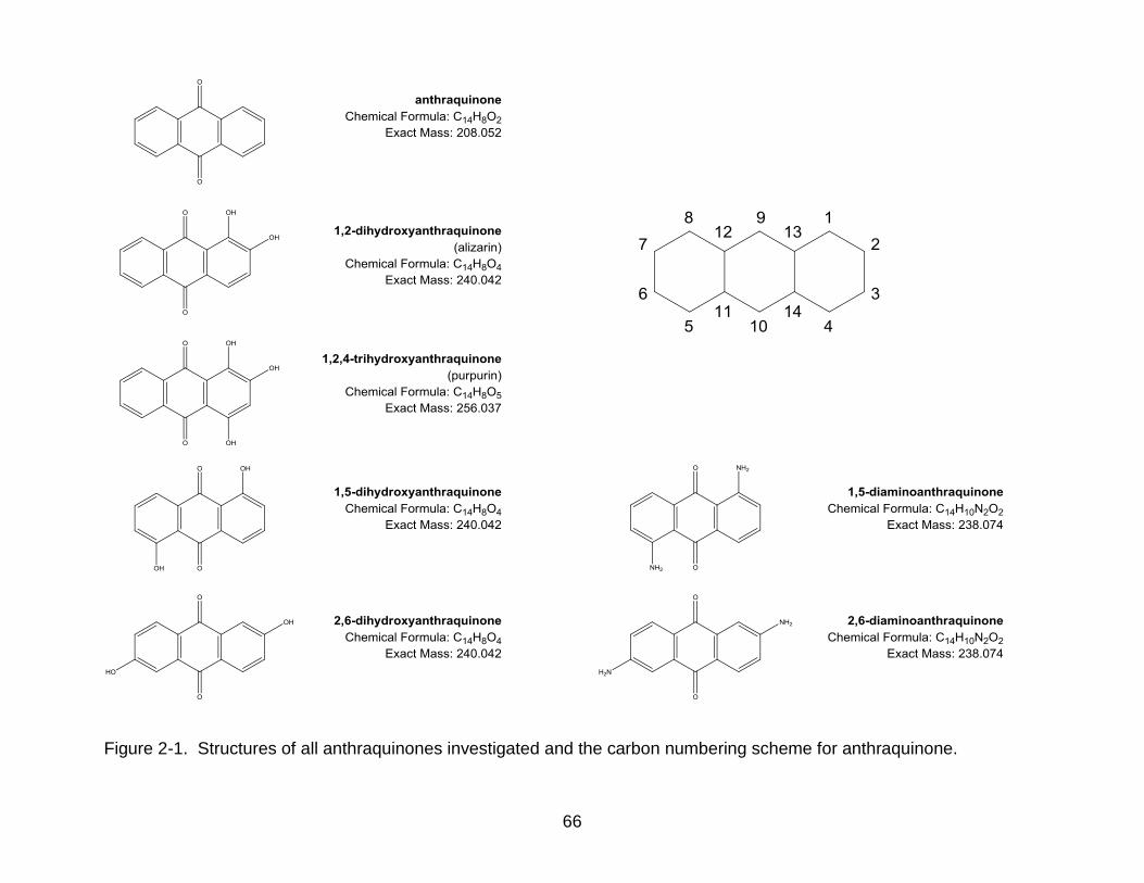
66
Figure 2-1. Structures of all anthraquinones investigated and the carbon numbering scheme for anthraquinone.
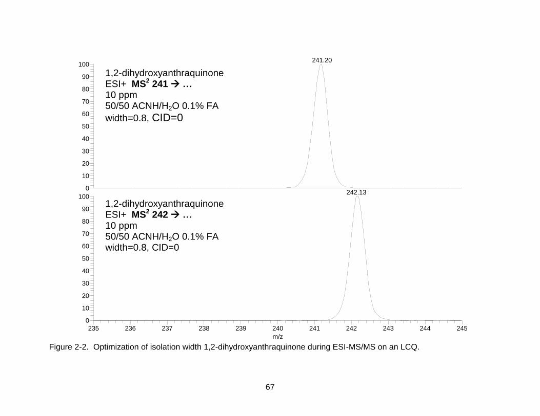
67
Figure 2-2. Optimization of isolation width 1,2-dihydroxyanthraquinone during ESI-MS/MS on an LCQ.
235 236 237 238 239 240 241 242 243 244 245
m/z
0
10
20
30
40
50
60
70
80
90
100
0
10
20
30
40
50
60
70
80
90
100
Rela
tive A
bundance
241.20
242.13
NL: 1.86E6
alizarin_ACN-H2O_FA_MS2_241-isolate#1-25 RT: 0.01-0.33 AV: 25 T: + p Full ms2 [email protected] [65.00-265.00]
NL: 4.03E5
alizarin_acn-h2o_fa_ms2_242-isolate#1-17 RT: 0.01-0.33 AV: 17 T: + p Full ms2 [email protected] [65.00-265.00]
1,2-dihydroxyanthraquinone ESI+ MS2 241 … 10 ppm 50/50 ACNH/H2O 0.1% FA
width=0.8, CID=0
1,2-dihydroxyanthraquinone ESI+ MS2 242 … 10 ppm 50/50 ACNH/H2O 0.1% FA width=0.8, CID=0
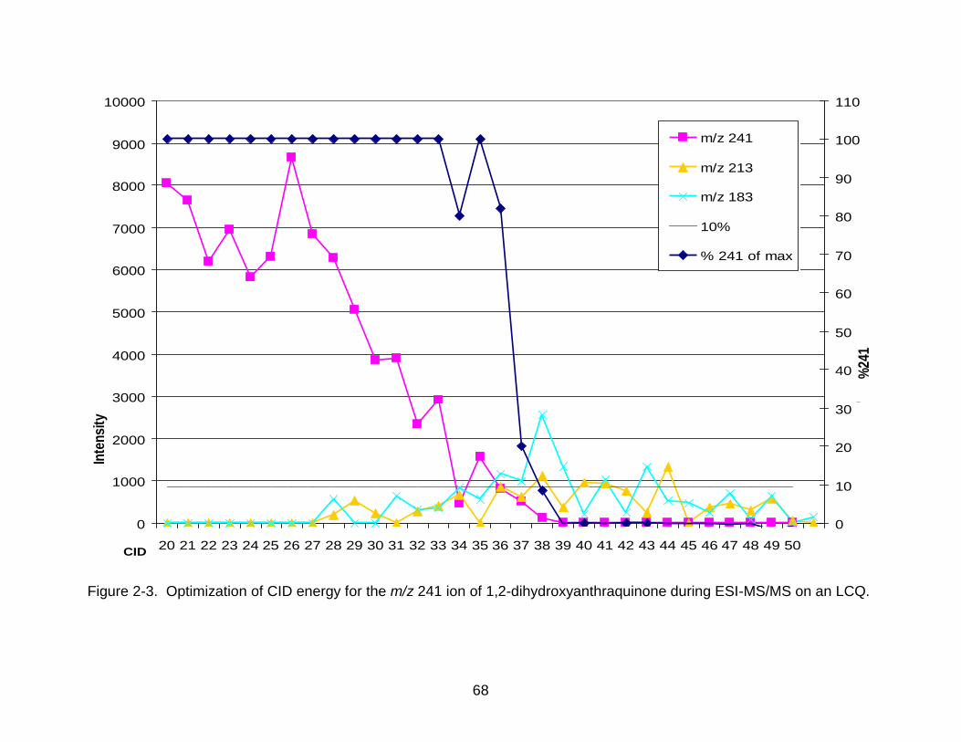
68
Figure 2-3. Optimization of CID energy for the m/z 241 ion of 1,2-dihydroxyanthraquinone during ESI-MS/MS on an LCQ.
1,2-dihydroxyanthraquinone ESI+ CID Optimization
0
1000
2000
3000
4000
5000
6000
7000
8000
9000
10000
20 21 22 23 24 25 26 27 28 29 30 31 32 33 34 35 36 37 38 39 40 41 42 43 44 45 46 47 48 49 50CID
Inte
nsi
ty
0
10
20
30
40
50
60
70
80
90
100
110
% 2
41
m/z 241
m/z 213
m/z 183
10%
% 241 of max
Inte
nsi
ty
%24
1
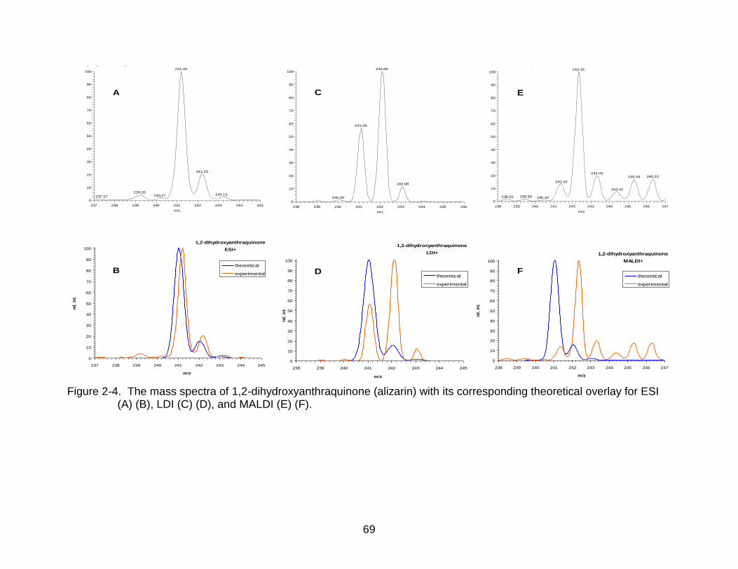
69
Figure 2-4. The mass spectra of 1,2-dihydroxyanthraquinone (alizarin) with its corresponding theoretical overlay for ESI (A) (B), LDI (C) (D), and MALDI (E) (F).
1,2-dihydroxyanthraquinone
ESI+
0
10
20
30
40
50
60
70
80
90
100
237 238 239 240 241 242 243 244 245
m/z
rel.
in
t.
theoretical
experimental
alizarin_ACN-H2O_FA #1-100 RT: 0.01-1.93 AV: 100 NL: 6.03E5
T: + p ms [100.00-1000.00]
237 238 239 240 241 242 243 244 245
m/z
0
10
20
30
40
50
60
70
80
90
100
Re
lativ
e A
bun
dan
ce
241.20
242.20
239.20243.13240.27237.27
A
B
alizarin_recrystallized_G7 #1-100 RT: 0.00-1.68 AV: 100 NL: 3.94E2
T: ITMS + p MALDI Full ms [50.00-1000.00]
238 239 240 241 242 243 244 245 246
m/z
0
10
20
30
40
50
60
70
80
90
100
Re
lativ
e A
bun
dan
ce
242.08
241.08
243.08
240.00
1,2-dihydroxyanthraquinone
LDI+
0
10
20
30
40
50
60
70
80
90
100
238 239 240 241 242 243 244 245
m/z
rel.
in
t.
theoretical
experimental
C
D
alizarin_10ppm_MALDI_F5 #1-100 RT: 0.00-1.34 AV: 100 NL: 3.09E4
T: ITMS + p MALDI Full ms [50.00-1000.00]
238 239 240 241 242 243 244 245 246 247
m/z
0
10
20
30
40
50
60
70
80
90
100
Re
lativ
e A
bun
dan
ce
242.33
243.33246.33245.33
241.42
244.42
239.50238.50 240.42
1,2-dihydroxyanthraquinone
MALDI+
0
10
20
30
40
50
60
70
80
90
100
238 239 240 241 242 243 244 245 246 247
m/z
rel.
in
t.
theoretical
experimental
E
F
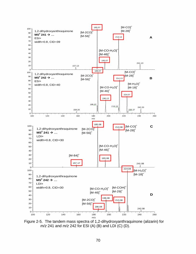
70
Figure 2-5. The tandem mass spectra of 1,2-dihydroxyanthraquinone (alizarin) for m/z 241 and m/z 242 for ESI (A) (B) and LDI (C) (D).
Alizarin, 10 ppm
50/50 ACNH/H2O 0.1% FA
ESI+ MS2 242 …
width=0.8, CID=40
Alizarin, 10 ppm
50/50 ACNH/H2O 0.1% FA
ESI+ MS2 241 …
width=0.8, CID=39
100 120 140 160 180 200 220 240 260
m/z
0
10
20
30
40
50
60
70
80
90
100
0
10
20
30
40
50
60
70
80
90
100
Rel
ativ
e A
bund
ance
185.07
213.13
195.07
241.13
157.13
186.07
214.13
224.07
196.13
185.07213.13
242.20
225.27158.20
NL: 2.72E5
alizarin_ACN-
H2O_FA_MS2_241#1-100
RT: 0.01-1.34 AV: 100 T: +
p Full ms2
[65.00-265.00]
NL: 3.02E4
alizarin_acn-
h2o_fa_ms2_242#1-65 RT:
0.00-1.34 AV: 65 T: + p
Full ms2 [email protected]
[65.00-265.00]
1,2-dihydroxyanthraquinone
MS2 241 …
ESI+
width=0.8, CID=39
1,2-dihydroxyanthraquinone
MS2 242 …
ESI+
width=0.8, CID=40
[M-CO-H2O]+
[M-46]+
[M-H2O]+
[M-18]+
A
B [M-2CO]
+
[M-56]+
[M-CO]+
[M-28]+
[M-CO-H2O]+
[M-46]+
[M-2CO]+
[M-56]+
[M-CO]+
[M-28]+
100 120 140 160 180 200 220 240 260
m/z
0
10
20
30
40
50
60
70
80
90
100
0
10
20
30
40
50
60
70
80
90
100
Rel
ativ
e A
bund
anc
e
185.08
213.08
195.08
157.17 241.08
224.08
196.08213.08
186.08242.08
NL: 1.40E2
alizarin_recrystallized_MS2_241_
nar_G7#1-50 RT: 0.00-0.87 AV:
50 T: ITMS + p MALDI Full ms2
[email protected] [65.00-265.00]
NL: 4.39E2
alizarin_recrystallized_ms2_242_
nar_g7#1-50 RT: 0.00-0.88 AV:
50 T: ITMS + p MALDI Full ms2
[email protected] [65.00-265.00]
1,2-dihydroxyanthraquinone
MS2 241 …
LDI+
width=0.8, CID=30
1,2-dihydroxyanthraquinone
MS2 242 …
LDI+
width=0.8, CID=30
C
D
[M-CO]+
[M-28]+ [M-2CO]
+
[M-56]+
[M-CO-H2O]+
[M-46]+
[M-84]+
[M-H2O]+
[M-18]+
[M-2CO]+
[M-56]+
[M-COH]+
[M-29]+
[M-CO-H2O]+
[M-46]+
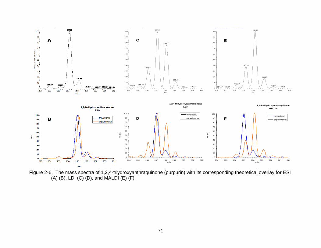
71
Figure 2-6. The mass spectra of 1,2,4-triydroxyanthraquinone (purpurin) with its corresponding theoretical overlay for ESI (A) (B), LDI (C) (D), and MALDI (E) (F).
purpurin_1000ppm_LDI_N20 #1-101 RT: 0.00-1.22 AV: 101 NL: 4.41E3
T: ITMS + p MALDI Full ms [100.00-1000.00]
254 255 256 257 258 259 260 261 262
m/z
0
10
20
30
40
50
60
70
80
90
100
Re
lativ
e A
bun
dan
ce
257.17
258.17
256.17
259.17
255.33254.25 260.17 261.17
1,2,4-trihydroxyanthraquinone
LDI+
0
10
20
30
40
50
60
70
80
90
100
254 255 256 257 258 259 260 261 262m/z
rel.
in
t.
theoretical
experimental
C
D
purpurin_1000ppm_MALDI_N22 #1-100 RT: 0.00-1.42 AV: 100 NL: 9.77E3
T: ITMS + p MALDI Full ms [100.00-1000.00]
254 255 256 257 258 259 260 261 262
m/z
0
10
20
30
40
50
60
70
80
90
100
Re
lativ
e A
bun
dan
ce
258.25
257.25
259.25
256.25
260.25261.25254.17 255.17
1,2,4-trihydroxyanthraquinone
MALDI+
0
10
20
30
40
50
60
70
80
90
100
254 255 256 257 258 259 260 261 262m/z
rel.
in
t.
theoretical
experimental
E
F
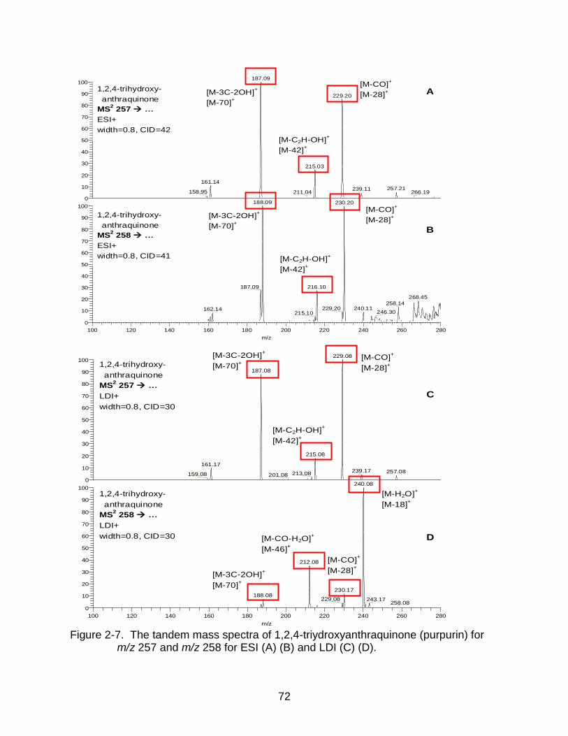
72
Figure 2-7. The tandem mass spectra of 1,2,4-triydroxyanthraquinone (purpurin) for m/z 257 and m/z 258 for ESI (A) (B) and LDI (C) (D).
100 120 140 160 180 200 220 240 260 280
m/z
0
10
20
30
40
50
60
70
80
90
100
0
10
20
30
40
50
60
70
80
90
100
Rel
ativ
e A
bund
ance
187.09
229.20
215.03
161.14
257.21239.11158.95 211.04 266.19
188.09 230.20
187.09 216.10
268.45
258.14229.20 240.11162.14
246.30215.10
NL: 1.59E5
Purpurin_ACN-
H2O_FA_MS2_257#1-100
RT: 0.01-1.38 AV: 100 T: +
p Full ms2
[70.00-290.00]
NL: 2.06E4
purpurin_acn-
h2o_fa_ms2_258#1-67 RT:
0.01-1.37 AV: 67 T: + p
Full ms2 [email protected]
[70.00-290.00]
1,2,4-trihydroxy-
anthraquinone
MS2 258 …
ESI+
width=0.8, CID=41
1,2,4-trihydroxy-
anthraquinone
MS2 257 …
ESI+
width=0.8, CID=42
A
B
[M-3C-2OH]+
[M-70]+
[M-C2H-OH]+
[M-42]+
[M-CO]+
[M-28]+
[M-CO]+
[M-28]+
[M-C2H-OH]+
[M-42]+
[M-3C-2OH]+
[M-70]+
100 120 140 160 180 200 220 240 260 280
m/z
0
10
20
30
40
50
60
70
80
90
100
0
10
20
30
40
50
60
70
80
90
100
Rel
ativ
e A
bund
ance
229.08
187.08
215.08
161.17
239.17 257.08213.08159.08 201.08
240.08
212.08
230.17188.08
229.08 243.17258.08
NL: 3.48E2
purpurin_1000ppm_LDI_MS2_2
57_N21#1-100 RT: 0.00-1.76
AV: 100 T: ITMS + p MALDI Full
[70.00-280.00]
NL: 3.95E2
purpurin_1000ppm_ldi_ms2_258
_n21#1-100 RT: 0.00-1.76 AV:
100 T: ITMS + p MALDI Full
[70.00-280.00]
1,2,4-trihydroxy-
anthraquinone
MS2 258 …
LDI+
width=0.8, CID=30
1,2,4-trihydroxy-
anthraquinone
MS2 257 …
LDI+
width=0.8, CID=30
C
D
[M-3C-2OH]+
[M-70]+
[M-CO]+
[M-28]+
[M-C2H-OH]+
[M-42]+
[M-CO-H2O]+
[M-46]+
[M-CO]+
[M-28]+
[M-H2O]+
[M-18]+
[M-3C-2OH]+
[M-70]+
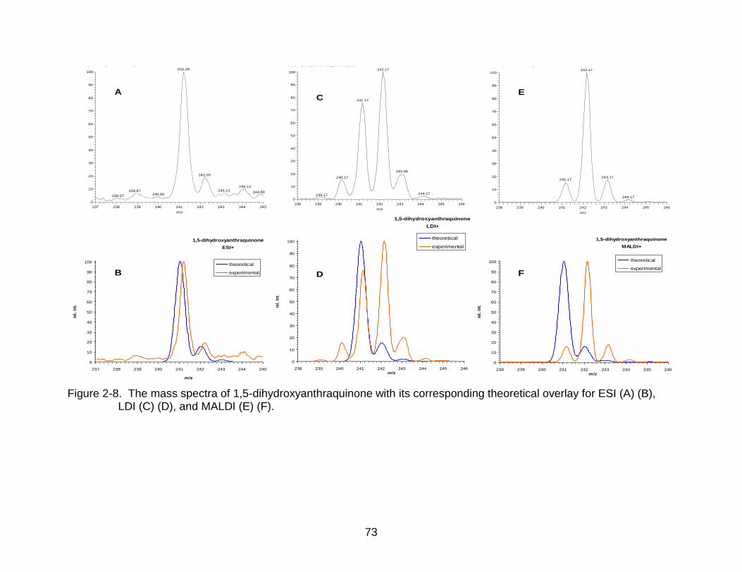
73
Figure 2-8. The mass spectra of 1,5-dihydroxyanthraquinone with its corresponding theoretical overlay for ESI (A) (B), LDI (C) (D), and MALDI (E) (F).
anthrarufin3_ACN-H2O_FA #1-100 RT: 0.01-2.04 AV: 100 NL: 3.92E4
T: + p Full ms [100.00-1000.00]
237 238 239 240 241 242 243 244 245
m/z
0
10
20
30
40
50
60
70
80
90
100
Re
lativ
e A
bun
dan
ce
241.20
242.20
244.13
243.13238.87 244.80240.00238.07
1,5-dihydroxyanthraquinone
ESI+
0
10
20
30
40
50
60
70
80
90
100
237 238 239 240 241 242 243 244 245
m/z
rel.
in
t.
theoretical
experimental
A
B
1,5-dihydroxyanthraquinone
LDI+
0
10
20
30
40
50
60
70
80
90
100
238 239 240 241 242 243 244 245 246m/z
rel.
in
t.
theoretical
experimental
anthrarufin_1500ppm_LDI_L20 #1-100 RT: 0.00-1.53 AV: 100 NL: 7.28E2
T: ITMS + p MALDI Full ms [100.00-1000.00]
238 239 240 241 242 243 244 245 246
m/z
0
10
20
30
40
50
60
70
80
90
100
Re
lativ
e A
bun
dan
ce
242.17
241.17
243.08
240.17
244.17239.17
C
D
anthrarufin_1500ppm_MALDI_L22 #1-100 RT: 0.00-1.45 AV: 100 NL: 1.57E4
T: ITMS + p MALDI Full ms [100.00-1000.00]
238 239 240 241 242 243 244 245 246
m/z
0
10
20
30
40
50
60
70
80
90
100
Re
lativ
e A
bun
dan
ce
242.17
243.17241.17
244.17
1,5-dihydroxyanthraquinone
MALDI+
0
10
20
30
40
50
60
70
80
90
100
238 239 240 241 242 243 244 245 246m/z
rel.
in
t.
theoretical
experimental
E
F
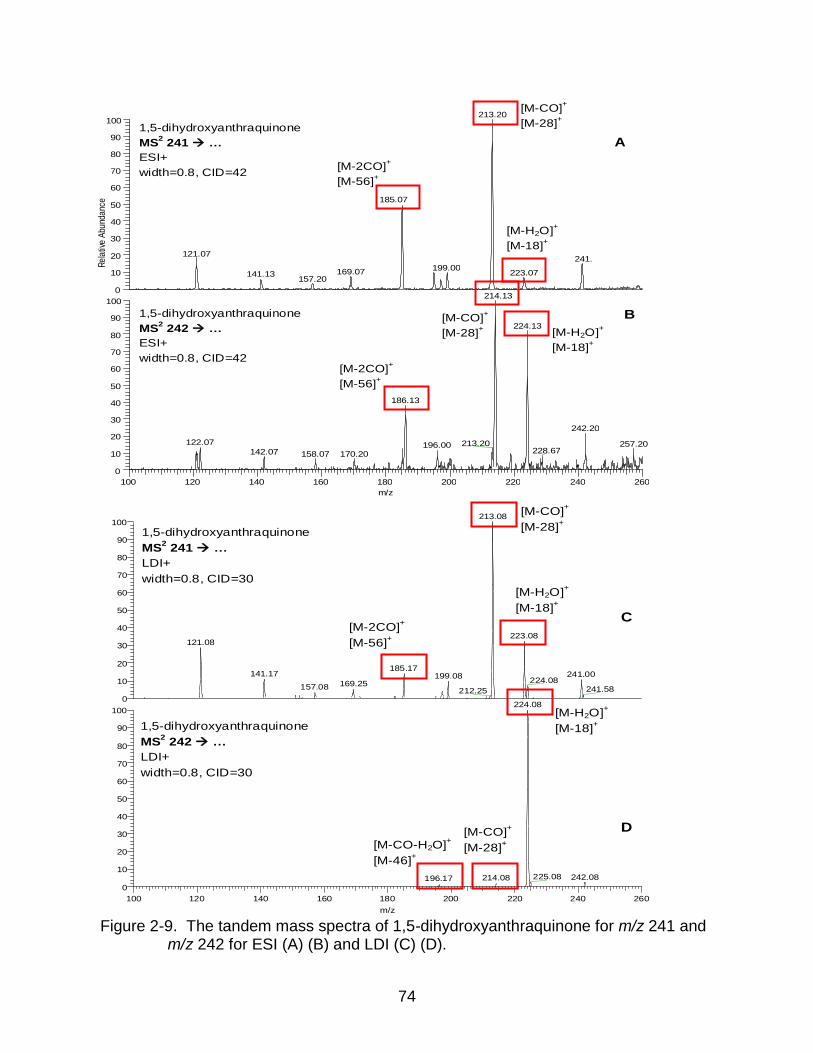
74
Figure 2-9. The tandem mass spectra of 1,5-dihydroxyanthraquinone for m/z 241 and m/z 242 for ESI (A) (B) and LDI (C) (D).
100 120 140 160 180 200 220 240 260 m/z
0
10
20
30
40
50
60
70
80
90
100 0
10
20
30
40
50
60
70
80
90
100
Re
lativ
e A
bund
anc
e
213.20
185.07
121.07 241.
199.00 169.07 223.07
141.13 157.20
224.13
186.13
242.20 122.07 213.20 257.20 196.00
228.67 142.07 170.20 158.07
214.13
1,5-dihydroxyanthraquinone
MS2 242 …
ESI+
width=0.8, CID=42
1,5-dihydroxyanthraquinone
MS2 241 …
ESI+
width=0.8, CID=42
A
B
[M-2CO]+
[M-56]+
[M-CO]+
[M-28]+ [M-H2O]
+
[M-18]+
[M-H2O]+
[M-18]+
[M-CO]+
[M-28]+
[M-2CO]+
[M-56]+
100 120 140 160 180 200 220 240 260
m/z
0
10
20
30
40
50
60
70
80
90
100
0
10
20
30
40
50
60
70
80
90
100
Rel
ativ
e A
bund
ance
213.08
223.08121.08
185.17141.17 241.00199.08
224.08169.25157.08 241.58212.25
224.08
225.08 242.08214.08196.17
NL: 3.23E1
anthrarufin_1500ppm_LDI_MS2_
241_L21#1-100 RT: 0.00-1.61
AV: 100 T: ITMS + p MALDI Full
[65.00-265.00]
NL: 8.60E2
anthrarufin_1500ppm_ldi_ms2_2
42_l21#1-100 RT: 0.00-1.60
AV: 100 T: ITMS + p MALDI Full
[65.00-265.00]
1,5-dihydroxyanthraquinone
MS2 242 …
LDI+
width=0.8, CID=30
1,5-dihydroxyanthraquinone
MS2 241 …
LDI+
width=0.8, CID=30
C
D
[M-2CO]+
[M-56]+
[M-CO-H2O]+
[M-46]+
[M-CO]+
[M-28]+
[M-H2O]+
[M-18]+
[M-H2O]+
[M-18]+
[M-CO]+
[M-28]+
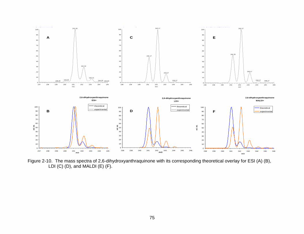
75
AnthraflavicAcid_ACN-H2O_FA #1-100 RT: 0.02-2.02 AV: 100 NL: 1.83E5
T: + p ms [100.00-1000.00]
237 238 239 240 241 242 243 244 245
m/z
0
10
20
30
40
50
60
70
80
90
100
Re
lativ
e A
bun
dan
ce
241.20
242.20
243.13
240.20 244.20239.20 245.00
2,6-dihydroxyanthraquinone
ESI+
0
10
20
30
40
50
60
70
80
90
100
237 238 239 240 241 242 243 244 245m/z
rel.
in
t.
theoretical
experimental
A
B
anthraflavic_acid_1000ppm_LDI_M20 #1-100 RT: 0.00-1.32 AV: 100 NL: 2.45E4
T: ITMS + p MALDI Full ms [100.00-1000.00]
238 239 240 241 242 243 244 245 246
m/z
0
10
20
30
40
50
60
70
80
90
100
Re
lativ
e A
bun
dan
ce
242.17
241.17
243.17
244.17
2,6-dihydroxyanthraquinone
LDI+
0
10
20
30
40
50
60
70
80
90
100
238 239 240 241 242 243 244 245 246m/z
rel.
in
t.
theoretical
experimental
C
D
anthraflavic_acid_1000ppm_MALDI_M22 #1-100 RT: 0.00-1.38 AV: 100 NL: 2.38E4
T: ITMS + p MALDI Full ms [100.00-1000.00]
238 239 240 241 242 243 244 245 246
m/z
0
10
20
30
40
50
60
70
80
90
100
Re
lativ
e A
bun
dan
ce
242.17
241.25
243.17
244.17 245.17
2,6-dihydroxyanthraquinone
MALDI+
0
10
20
30
40
50
60
70
80
90
100
238 239 240 241 242 243 244 245 246
m/z
rel.
in
t.
theoretical
experimental
E
F
Figure 2-10. The mass spectra of 2,6-dihydroxyanthraquinone with its corresponding theoretical overlay for ESI (A) (B), LDI (C) (D), and MALDI (E) (F).
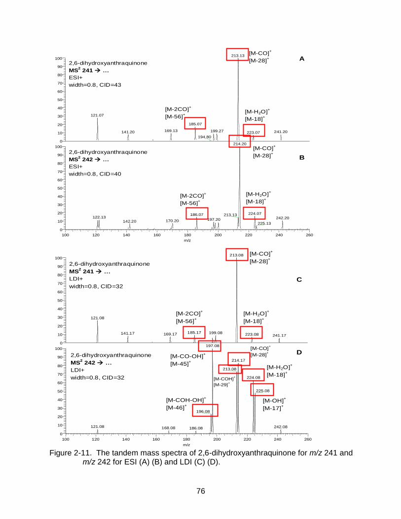
76
Figure 2-11. The tandem mass spectra of 2,6-dihydroxyanthraquinone for m/z 241 and m/z 242 for ESI (A) (B) and LDI (C) (D).
100 120 140 160 180 200 220 240 260
m/z
0
10
20
30
40
50
60
70
80
90
100
0
10
20
30
40
50
60
70
80
90
100
Rel
ativ
e A
bund
ance
213.13
121.07
185.07
169.13 199.27 241.20141.20 223.07
194.80
214.20
224.07186.07 213.13122.13 242.20197.20170.20142.20
225.13
NL: 5.74E4
AnthraflavicAcid_ACN-
H2O_FA_MS2_241#1-100
RT: 0.01-1.39 AV: 100 T: + p
Full ms2 [email protected]
[65.00-270.00]
NL: 1.12E4
anthraflavicacid_acn-
h2o_fa_ms2_242#1-100 RT:
0.01-2.09 AV: 100 T: + p Full
[65.00-270.00]
2,6-dihydroxyanthraquinone
MS2 242 …
ESI+
width=0.8, CID=40
2,6-dihydroxyanthraquinone
MS2 241 …
ESI+
width=0.8, CID=43
A
B
[M-2CO]+
[M-56]+
[M-H2O]+
[M-18]+
[M-CO]+
[M-28]+
[M-H2O]+
[M-18]+
[M-CO]+
[M-28]+
[M-2CO]+
[M-56]+
100 120 140 160 180 200 220 240 260
m/z
0
10
20
30
40
50
60
70
80
90
100
0
10
20
30
40
50
60
70
80
90
100
Rel
ativ
e A
bund
ance
213.08
121.08
185.17 199.08141.17 169.17 223.08 241.17
197.08
214.17
213.08
224.08
225.08
196.08
121.08 242.08168.08 186.08
NL: 3.24E2
anthraflavic_acid_1000ppm_LDI_M
S2_241_M21#1-100 RT:
0.00-1.60 AV: 100 T: ITMS + p
MALDI Full ms2 [email protected]
[65.00-265.00]
NL: 7.85E2
anthraflavic_acid_1000ppm_ldi_ms
2_242_m21#1-100 RT: 0.00-1.61
AV: 100 T: ITMS + p MALDI Full
[65.00-265.00]
2,6-dihydroxyanthraquinone
MS2 242 …
LDI+
width=0.8, CID=32
2,6-dihydroxyanthraquinone
MS2 241 …
LDI+
width=0.8, CID=32
C
D
[M-2CO]+
[M-56]+
[M-CO-OH]+
[M-45]+
[M-COH-OH]+
[M-46]+
[M-COH]+
[M-29]+
[M-CO]+
[M-28]+
[M-H2O]+
[M-18]+
[M-OH]+
[M-17]+
[M-H2O]+
[M-18]+
[M-CO]+
[M-28]+
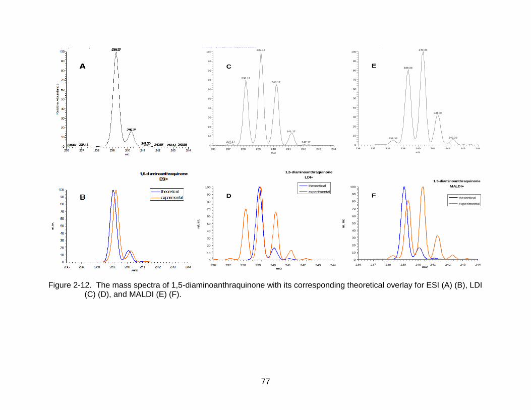
77
Figure 2-12. The mass spectra of 1,5-diaminoanthraquinone with its corresponding theoretical overlay for ESI (A) (B), LDI (C) (D), and MALDI (E) (F).
1,5-diaminoanthraquinone_1000ppm_LDI_M17 #1-100 RT: 0.00-1.50 AV: 100 NL: 1.40E4
T: ITMS + p MALDI Full ms [100.00-1000.00]
236 237 238 239 240 241 242 243 244
m/z
0
10
20
30
40
50
60
70
80
90
100
Re
lativ
e A
bun
dan
ce
239.17
238.17
240.17
241.17
237.17 242.17
1,5-diaminoanthraquinone
LDI+
0
10
20
30
40
50
60
70
80
90
100
236 237 238 239 240 241 242 243 244
m/z
rel.
in
t.
theoretical
experimental
C
D
1,5-diaminoanthraquinone_1000ppm_MALDI_M19 #1-100 RT: 0.00-1.46 AV: 100 NL: 6.61E4
T: ITMS + p MALDI Full ms [100.00-1000.00]
236 237 238 239 240 241 242 243 244
m/z
0
10
20
30
40
50
60
70
80
90
100
Re
lativ
e A
bun
dan
ce
240.33
239.33
241.33
242.33238.33
1,5-diaminoanthraquinone
MALDI+
0
10
20
30
40
50
60
70
80
90
100
236 237 238 239 240 241 242 243 244m/z
rel.
in
t.
theoretical
experimental
E
F
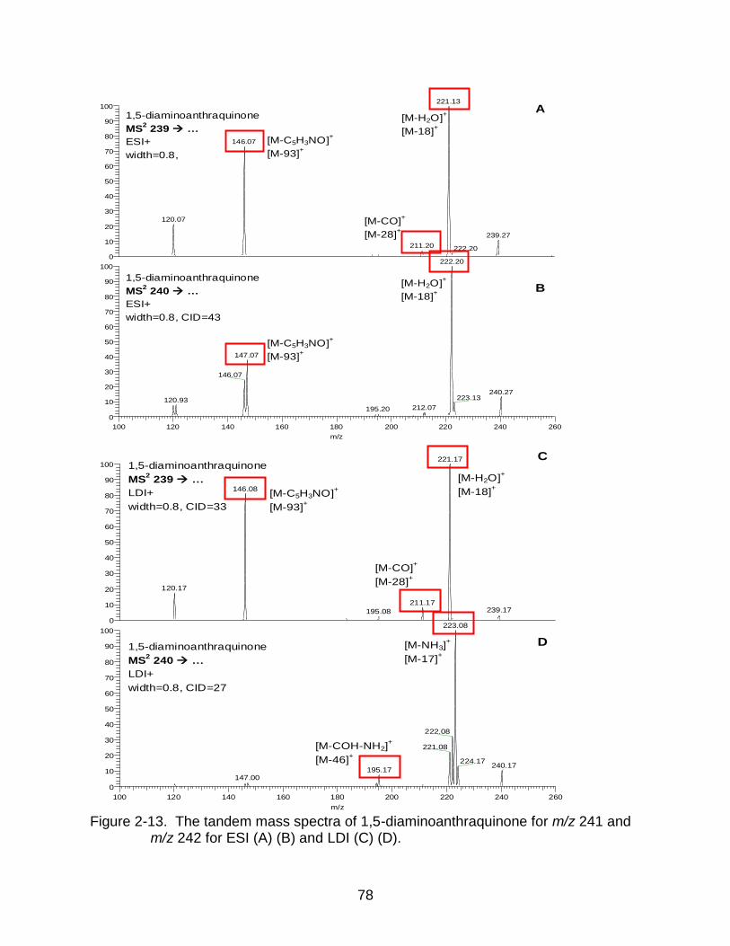
78
Figure 2-13. The tandem mass spectra of 1,5-diaminoanthraquinone for m/z 241 and m/z 242 for ESI (A) (B) and LDI (C) (D).
100 120 140 160 180 200 220 240 260
m/z
0
10
20
30
40
50
60
70
80
90
100
0
10
20
30
40
50
60
70
80
90
100
Rel
ativ
e A
bund
ance
221.17
146.08
120.17
211.17239.17195.08
223.08
222.08
221.08
224.17240.17
195.17147.00
NL: 1.28E2
1,5-
diaminoanthraquinone_1000ppm_LD
I_MS2_239_M18#1-100 RT:
0.00-1.76 AV: 100 T: ITMS + p
MALDI Full ms2 [email protected]
[65.00-260.00]
NL: 4.49E2
1,5-
diaminoanthraquinone_1000ppm_ldi
_ms2_240_m18#1-99 RT:
0.00-1.76 AV: 99 T: ITMS + p
MALDI Full ms2 [email protected]
[65.00-260.00]
1,5-diaminoanthraquinone
MS2 240 …
LDI+
width=0.8, CID=27
C
D
1,5-diaminoanthraquinone
MS2 239 …
LDI+
width=0.8, CID=33
[M-H2O]+
[M-18]+
[M-C5H3NO]+
[M-93]+
[M-CO]+
[M-28]+
[M-NH3]+
[M-17]+
[M-COH-NH2]+
[M-46]+
100 120 140 160 180 200 220 240 260
m/z
0
10
20
30
40
50
60
70
80
90
100
0
10
20
30
40
50
60
70
80
90
100
Rel
ativ
e A
bund
ance
221.13
146.07
120.07
239.27
211.20 222.20
222.20
147.07
146.07
240.27223.13120.93
212.07195.20
NL: 6.06E4
1,5-diaminoanthraquinone_ACN-
H2O_FA_MS2_239#1-100 RT:
0.01-1.49 AV: 100 T: + p Full
[65.00-270.00]
NL: 6.38E3
1,5-diaminoanthraquinone_acn-
h2o_fa_ms2_240#1-100 RT:
0.02-2.17 AV: 100 T: + p Full
[65.00-270.00]
1,5-diaminoanthraquinone
MS2 240 …
ESI+
width=0.8, CID=43
1,5-diaminoanthraquinone
MS2 239 …
ESI+
width=0.8,
A
B [M-H2O]
+
[M-18]+
[M-CO]+
[M-28]+
[M-H2O]+
[M-18]+
[M-C5H3NO]+
[M-93]+
[M-C5H3NO]+
[M-93]+
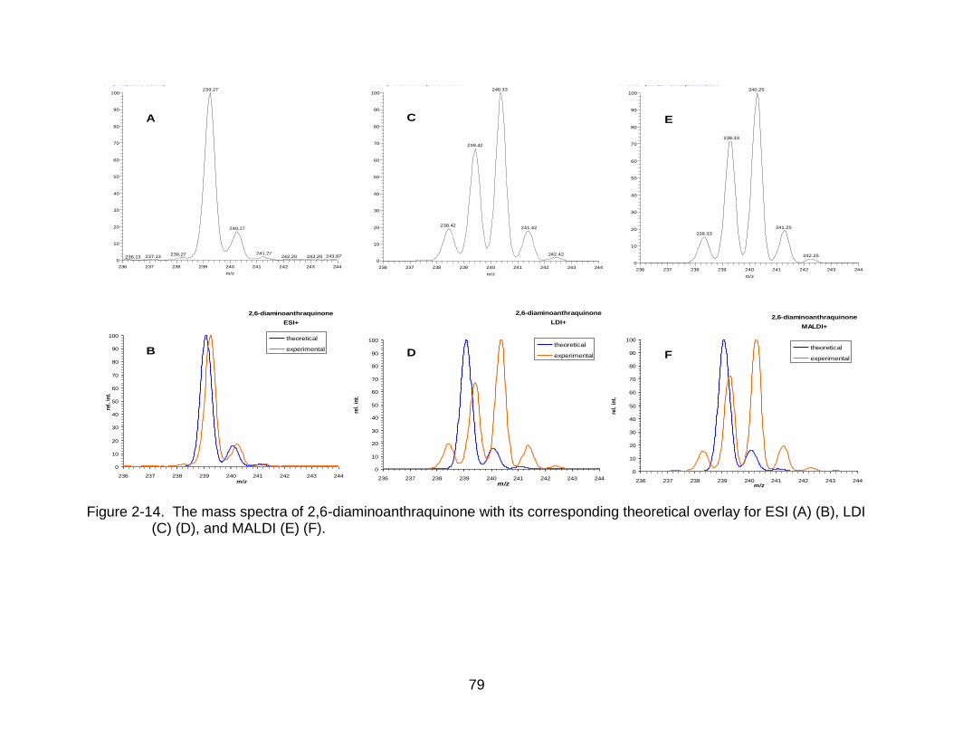
79
Figure 2-14. The mass spectra of 2,6-diaminoanthraquinone with its corresponding theoretical overlay for ESI (A) (B), LDI (C) (D), and MALDI (E) (F).
2,6-diaminoanthraquinone_ACN-H2O_FA #1-100 RT: 0.01-1.89 AV: 100 NL: 1.23E6
T: + p ms [100.00-1000.00]
236 237 238 239 240 241 242 243 244
m/z
0
10
20
30
40
50
60
70
80
90
100
Re
lativ
e A
bun
dan
ce
239.27
240.27
241.27238.27 243.87242.20 243.20237.13236.13
2,6-diaminoanthraquinone
ESI+
0
10
20
30
40
50
60
70
80
90
100
236 237 238 239 240 241 242 243 244m/z
rel.
in
t.
theoretical
experimental
A
B
2,6-diaminoanthraquinone_1500ppm_LDI_L17 #1-100 RT: 0.00-1.05 AV: 100 NL: 5.09E5
T: ITMS + p MALDI Full ms [100.00-1000.00]
236 237 238 239 240 241 242 243 244
m/z
0
10
20
30
40
50
60
70
80
90
100
Re
lativ
e A
bun
dan
ce
240.33
239.42
238.42241.42
242.42
2,6-diaminoanthraquinone
LDI+
0
10
20
30
40
50
60
70
80
90
100
236 237 238 239 240 241 242 243 244m/z
rel.
in
t.
theoretical
experimental
C
D
2,6-diaminoanthraquinone_1500ppm_MALDI_L19 #1-100 RT: 0.00-1.43 AV: 100 NL: 7.63E4
T: ITMS + p MALDI Full ms [100.00-1000.00]
236 237 238 239 240 241 242 243 244
m/z
0
10
20
30
40
50
60
70
80
90
100
Re
lativ
e A
bun
dan
ce
240.25
239.33
241.25
238.33
242.25
2,6-diaminoanthraquinone
MALDI+
0
10
20
30
40
50
60
70
80
90
100
236 237 238 239 240 241 242 243 244m/z
rel.
in
t.
theoretical
experimental
E
F
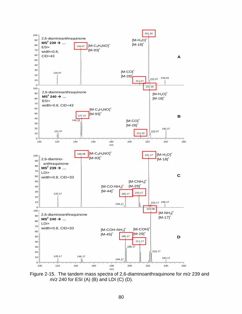
80
Figure 2-15. The tandem mass spectra of 2,6-diaminoanthraquinone for m/z 239 and m/z 240 for ESI (A) (B) and LDI (C) (D).
100 120 140 160 180 200 220 240 260
m/z
0
10
20
30
40
50
60
70
80
90
100
0
10
20
30
40
50
60
70
80
90
100
Rel
ativ
e A
bund
ance
221.20
146.07
120.07
239.20222.07
211.27
222.20
147.13
146.13
240.27121.07 223.07
212.20
NL: 2.48E5
2,6-diaminoanthraquinone_ACN-
H2O_FA_MS2_239#1-100 RT:
0.01-1.25 AV: 100 T: + p Full
[65.00-270.00]
NL: 4.32E4
2,6-diaminoanthraquinone_acn-
h2o_fa_ms2_240#1-100 RT:
0.02-1.64 AV: 100 T: + p Full
[65.00-270.00]
2,6-diaminoanthraquinone
MS2 240 …
ESI+
width=0.8, CID=43
2,6-diaminoanthraquinone
MS2 239 …
ESI+
width=0.8,
CID=43 A
B
[M-C5H3NO]+
[M-93]+
[M-CO]+
[M-28]+
[M-H2O]+
[M-18]+
[M-CO]+
[M-28]+
[M-H2O]+
[M-18]+ [M-C5H3NO]
+
[M-93]+
100 120 140 160 180 200 220 240 260
m/z
0
10
20
30
40
50
60
70
80
90
100
0
10
20
30
40
50
60
70
80
90
100
Rel
ativ
e A
bund
ance
146.08221.17
210.17120.17 195.17
239.17223.17194.17
223.08
195.17
211.17
196.17
224.17
120.17 146.17240.17
194.17
NL: 1.57E4
2,6-
diaminoanthraquinone_1500ppm_LD
I_MS2_239_L18#1-100 RT:
0.00-1.78 AV: 100 T: ITMS + p
MALDI Full ms2 [email protected]
[65.00-260.00]
NL: 2.64E4
2,6-
diaminoanthraquinone_1500ppm_ldi
_ms2_240_l18#1-100 RT: 0.00-1.73
AV: 100 T: ITMS + p MALDI Full
[65.00-260.00]
C
D
2,6-diamino-
anthraquinone
MS2 239 …
LDI+
width=0.8, CID=33
2,6-diaminoanthraquinone
MS2 240 …
LDI+
width=0.8, CID=33
[M-NH3]+
[M-17]+
[M-COH-NH2]+
[M-45]+
[M-C5H3NO]+
[M-93]+
[M-CO-NH2]+
[M-44]+
[M-CNH3]+
[M-29]+
[M-H2O]+
[M-18]+
[M-COH]+
[M-29]+
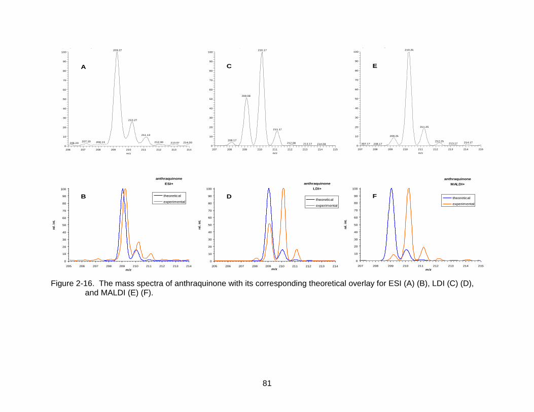
81
Figure 2-16. The mass spectra of anthraquinone with its corresponding theoretical overlay for ESI (A) (B), LDI (C) (D), and MALDI (E) (F).
anthraquinone
ESI+
0
10
20
30
40
50
60
70
80
90
100
205 206 207 208 209 210 211 212 213 214
m/z
rel.
in
t.
theoretical
experimental
Anthraquinone_ACN-H2O_FA_TFA-blewdown #1-100 RT: 0.02-2.01 AV: 100 NL: 1.52E5
T: + p ms [100.00-1000.00]
206 207 208 209 210 211 212 213 214
m/z
0
10
20
30
40
50
60
70
80
90
100
Re
lativ
e A
bun
dan
ce
209.27
210.27
211.13
207.20 208.13 212.00 214.00213.07206.20
A
B
anthraquinone_unrecry_acetone_LDI_G11 #1-100 RT: 0.00-1.68 AV: 100 NL: 1.54E3
T: ITMS + p MALDI Full ms [50.00-1000.00]
207 208 209 210 211 212 213 214 215
m/z
0
10
20
30
40
50
60
70
80
90
100
Re
lativ
e A
bun
dan
ce
210.17
209.08
211.17
208.17212.08 213.17 214.08
anthraquinone
LDI+
0
10
20
30
40
50
60
70
80
90
100
205 206 207 208 209 210 211 212 213 214m/z
rel.
in
t.theoretical
experimental
C
D
anthraquinone_unrecry_acetone_MALDI_DHB_G12 #1-101 RT: 0.00-1.56 AV: 101 NL: 9.15E3
T: ITMS + p MALDI Full ms [50.00-1000.00]
207 208 209 210 211 212 213 214 215
m/z
0
10
20
30
40
50
60
70
80
90
100
Re
lativ
e A
bun
dan
ce
210.25
211.25
209.25
212.25214.17213.17207.17 208.17
anthraquinone
MALDI+
0
10
20
30
40
50
60
70
80
90
100
207 208 209 210 211 212 213 214 215
m/z
rel.
in
t.
theoretical
experimental
E
F
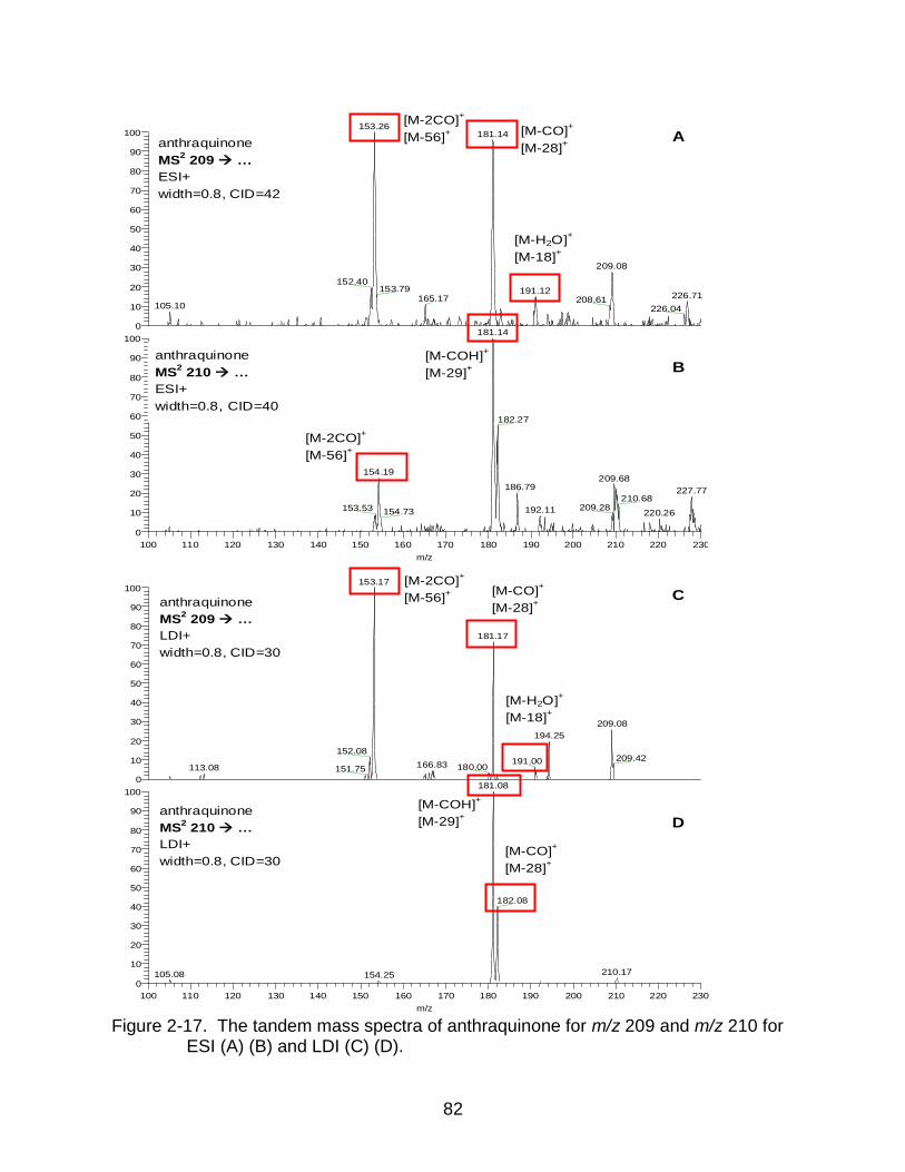
82
Figure 2-17. The tandem mass spectra of anthraquinone for m/z 209 and m/z 210 for ESI (A) (B) and LDI (C) (D).
100 110 120 130 140 150 160 170 180 190 200 210 220 230
m/z
0
10
20
30
40
50
60
70
80
90
100
0
10
20
30
40
50
60
70
80
90
100
Rel
ativ
e A
bund
ance
153.26181.14
209.08
152.40153.79 191.12
226.71165.17 208.61105.10 226.04
181.14
182.27
154.19209.68
186.79 227.77210.68
209.28153.53 192.11154.73 220.26
NL: 1.64E3
Anthraquinone_ACN-
H2O_FA_TFA-
blewdown_MS2_209_CID42#1-
50 RT: 0.00-1.05 AV: 50 T: + p
Full ms2 [email protected]
[55.00-240.00]
NL: 1.16E3
anthraquinone_acn-h2o_fa_tfa-
blewdown_ms2_210_cid40#1-50
RT: 0.00-1.05 AV: 50 T: + p Full
[55.00-240.00]
A
B
anthraquinone
MS2 209 …
ESI+
width=0.8, CID=42
anthraquinone
MS2 210 …
ESI+
width=0.8, CID=40
[M-2CO]+
[M-56]+
[M-CO]+
[M-28]+
[M-H2O]+
[M-18]+
[M-COH]+
[M-29]+
[M-2CO]+
[M-56]+
100 110 120 130 140 150 160 170 180 190 200 210 220 230
m/z
0
10
20
30
40
50
60
70
80
90
100
0
10
20
30
40
50
60
70
80
90
100
Rel
ativ
e A
bund
ance
153.17
181.17
209.08
194.25
152.08209.42191.00166.83 180.00113.08 151.75
181.08
182.08
210.17105.08 154.25
NL: 3.75
anthraquinone_LDI_MS2_209_G
11#1-100 RT: 0.00-2.23 AV:
100 T: ITMS + p MALDI Full
[55.00-235.00]
NL: 7.49E1
anthraquinone_ldi_ms2_210_nar
_g11#1-100 RT: 0.00-1.79 AV:
100 T: ITMS + p MALDI Full
[55.00-245.00]
anthraquinone
MS2 209 …
LDI+
width=0.8, CID=30
anthraquinone
MS2 210 …
LDI+
width=0.8, CID=30
C
D
[M-H2O]+
[M-18]+
[M-CO]+
[M-28]+
[M-2CO]+
[M-56]+
[M-COH]+
[M-29]+
[M-CO]+
[M-28]+
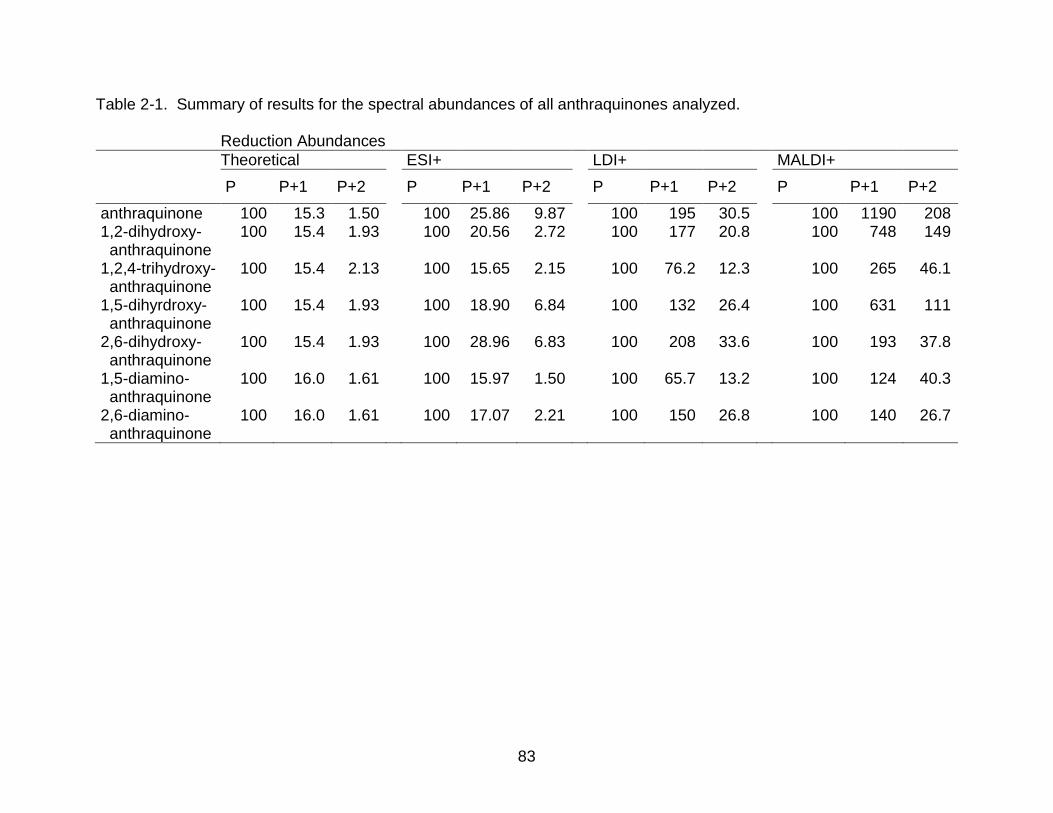
83
Table 2-1. Summary of results for the spectral abundances of all anthraquinones analyzed. Reduction Abundances
Theoretical ESI+ LDI+ MALDI+
P P+1 P+2 P P+1 P+2 P P+1 P+2 P P+1 P+2
anthraquinone 100 15.3 1.50 100 25.86 9.87 100 195 30.5 100 1190 208 1,2-dihydroxy- anthraquinone
100 15.4 1.93 100 20.56 2.72 100 177 20.8 100 748 149
1,2,4-trihydroxy- anthraquinone
100 15.4 2.13 100 15.65 2.15 100 76.2 12.3 100 265 46.1
1,5-dihyrdroxy- anthraquinone
100 15.4 1.93 100 18.90 6.84 100 132 26.4 100 631 111
2,6-dihydroxy- anthraquinone
100 15.4 1.93 100 28.96 6.83 100 208 33.6 100 193 37.8
1,5-diamino- anthraquinone
100 16.0 1.61 100 15.97 1.50 100 65.7 13.2 100 124 40.3
2,6-diamino- anthraquinone
100 16.0 1.61 100 17.07 2.21 100 150 26.8 100 140 26.7
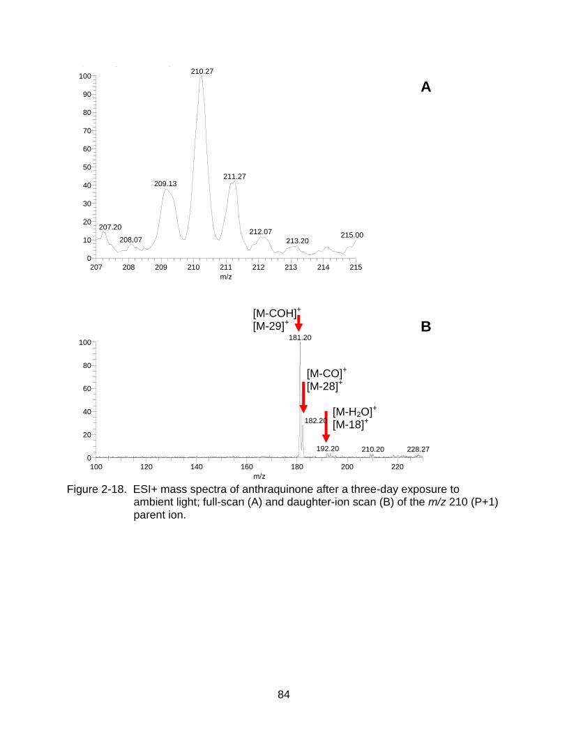
84
Figure 2-18. ESI+ mass spectra of anthraquinone after a three-day exposure to ambient light; full-scan (A) and daughter-ion scan (B) of the m/z 210 (P+1) parent ion.
Anthraquinone_10ppm_FA #1-100 RT: 0.01-1.85 AV: 100 NL: 6.45E4T: + p Full ms [100.00-1000.00]
207 208 209 210 211 212 213 214 215
m/z
0
10
20
30
40
50
60
70
80
90
100
Re
lative
Ab
un
da
nce
210.27
211.27209.13
207.20212.07 215.00
208.07 213.20
Anthraquinone_10ppm_FA_MS2_210 #1-100 RT: 0.02-2.09 AV: 100 NL: 9.51E3T: + p Full ms2 [email protected] [55.00-235.00]
100 120 140 160 180 200 220
m/z
0
20
40
60
80
100
Re
lative
Ab
un
da
nce
181.20
182.20
192.20 228.27210.20
[M-H2O]+ [M-18]+
[M-CO]+ [M-28]+
[M-COH]+ [M-29]+
A
B
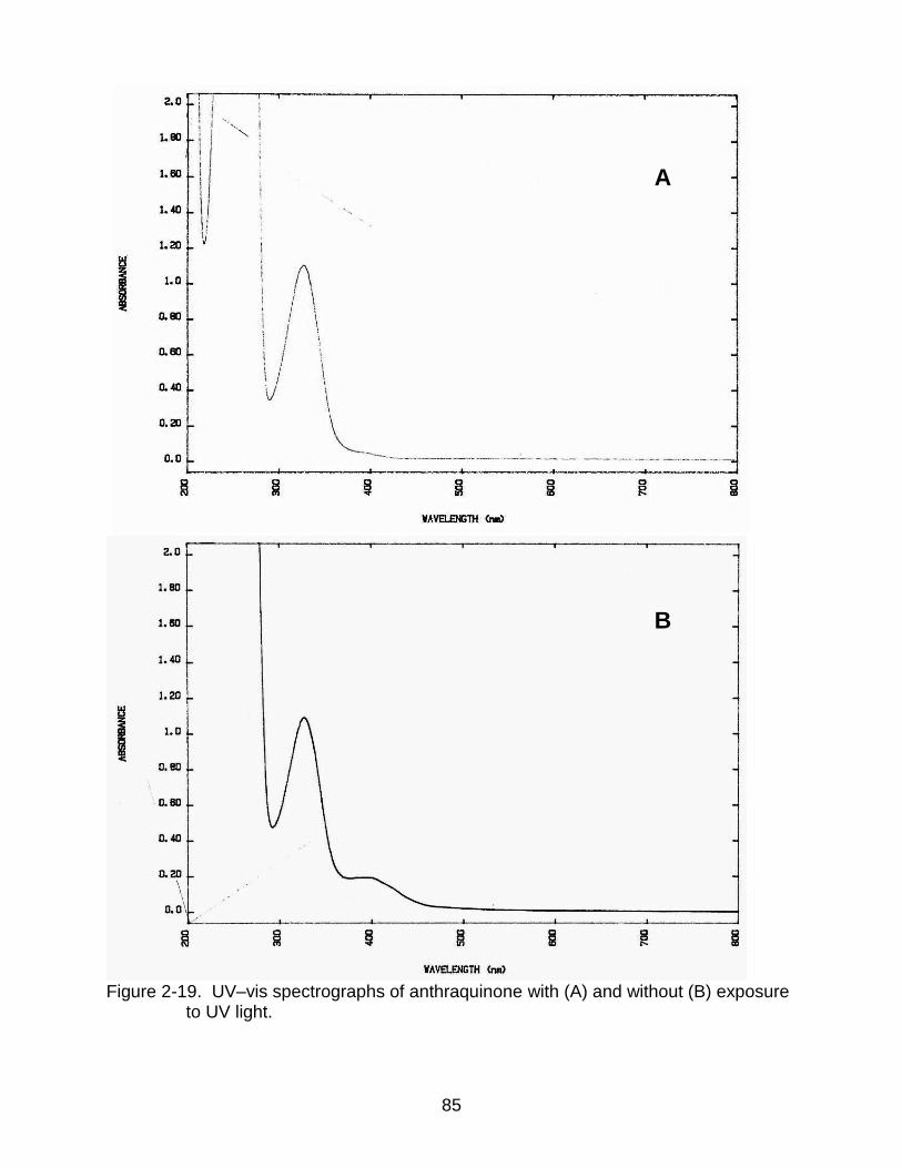
85
Figure 2-19. UV–vis spectrographs of anthraquinone with (A) and without (B) exposure to UV light.
A
B
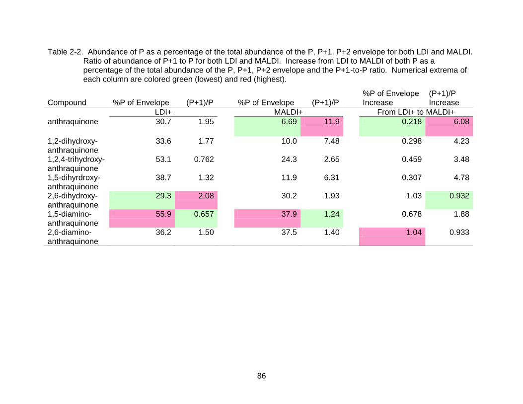
86
Table 2-2. Abundance of P as a percentage of the total abundance of the P, P+1, P+2 envelope for both LDI and MALDI. Ratio of abundance of P+1 to P for both LDI and MALDI. Increase from LDI to MALDI of both P as a percentage of the total abundance of the P, P+1, P+2 envelope and the P+1-to-P ratio. Numerical extrema of each column are colored green (lowest) and red (highest).
Compound %P of Envelope (P+1)/P %P of Envelope (P+1)/P %P of Envelope Increase
(P+1)/P Increase
LDI+ MALDI+ From LDI+ to MALDI+
anthraquinone 30.7 1.95 6.69 11.9 0.218 6.08
1,2-dihydroxy- anthraquinone
33.6 1.77 10.0 7.48 0.298 4.23
1,2,4-trihydroxy- anthraquinone
53.1 0.762 24.3 2.65 0.459 3.48
1,5-dihyrdroxy- anthraquinone
38.7 1.32 11.9 6.31 0.307 4.78
2,6-dihydroxy- anthraquinone
29.3 2.08 30.2 1.93 1.03 0.932
1,5-diamino- anthraquinone
55.9 0.657 37.9 1.24 0.678 1.88
2,6-diamino- anthraquinone
36.2 1.50 37.5 1.40 1.04 0.933
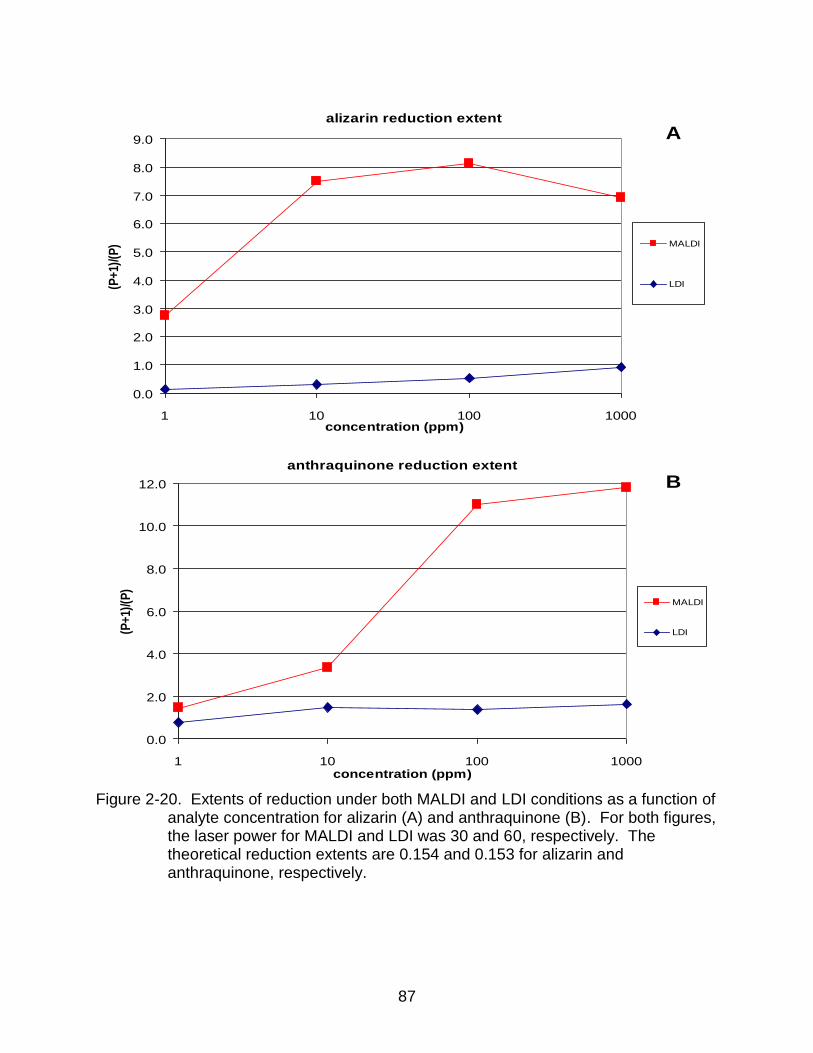
87
Figure 2-20. Extents of reduction under both MALDI and LDI conditions as a function of analyte concentration for alizarin (A) and anthraquinone (B). For both figures, the laser power for MALDI and LDI was 30 and 60, respectively. The theoretical reduction extents are 0.154 and 0.153 for alizarin and anthraquinone, respectively.
anthraquinone reduction extent
0.0
2.0
4.0
6.0
8.0
10.0
12.0
1 10 100 1000concentration (ppm)
(P+
1)/(
P)
MALDI
LDI
alizarin reduction extent
0.0
1.0
2.0
3.0
4.0
5.0
6.0
7.0
8.0
9.0
1 10 100 1000concentration (ppm)
(P+
1)/(
P) MALDI
LDI
B
A (P
+1)
/(P
)
(P+
1)/(
P)
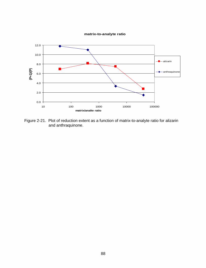
88
Figure 2-21. Plot of reduction extent as a function of matrix-to-analyte ratio for alizarin and anthraquinone.
matrix-to-analyte ratio
0.0
2.0
4.0
6.0
8.0
10.0
12.0
10 100 1000 10000 100000
matrix/analte ratio
(P+
1)/(
P)
alizarin
anthraquinone
(P+
1)/(
P)
89
CHAPTER 3 TANDEM MASS SPECTROMETRY OF CLUSTERS FROM LEAD WHITE
Background
The use and history of lead is inextricably tied to the developments of metallurgy,
art, geology, archaeology, and mass spectrometry. The earliest uses of lead in its
elemental, metallic form can be traced to circa 6,000 B.C. in the Balkans and Near East,
circa 1,500 B.C. in Egypt where it was mixed with tin to form pewter, and the Roman
Empire where it was extensively used as a conduit for water (indeed, the term
“plumbing” is derived from the Latin plumbum).3
Regarding lead in artistic objects, it has seen use as galena (PbS) for the ancient
Egyptian eye makeup known as black kohl2, in Greek and Roman bronze coins and
statues117,118, as litharge and massicot (PbO) for ancient and Art Nouveau glass119, and
as cames for medieval stained glass117. Arguably, lead’s most important artistic role
has been in the pigment known as either lead white or flake white ((PbCO3)2•Pb(OH)2).
Lead white may also be called hydrocerussite, which is a rarer form of the mineral
cerussite (lead carbonate, PbCO3), but its use as a pigment stems from synthetic roots.
Lead white has been in use as a pigment for at least two millennia: there are accounts
of its use in China, circa 300 B.C., and ancient Greece and Rome where Pliny
documented its synthesis.50,117 Indeed, lead white is one of the oldest known pigments
synthetically produced and was the only white pigment used in painted works of art until
the twentieth century development of safer substitutes, such as ZnO and TiO2.50,120 The
process of preparing lead white consists of suspending strips of metallic lead over
vinegar (acetic acid, CH3COOH) in clay pots stored in a shed with horse manure, to
supply carbon dioxide (CO2). After several weeks, the exterior flakes of lead white are
90
scraped off and pulverized.50 Though less frequently used, Naples yellow is another
artistic pigment based on lead, found in the natural mineral lead antimonate (Pb2Sb2O7).
Four other lead-containing pigments are chrome orange (PbCrO4•Pb(OH)2), chrome
yellow (PbCrO4), lead-tin yellow (Pb2SnO4 or Pb(Sn,Si)O3), and red lead (Pb3O4).
In addition to galena, litharge/massicot, and cerussite (vide supra), six other
minerals have historically been used for the smelting of lead: anglesite (PbSO4),
boulangerite (Pb5Sb4S11), bournonite (CuPbSbS3), laurionite (Pb(OH)Cl), phosgenite
(Pb2(CO3)Cl2), and semseyite (Pb9Sb8S21).3 It is from these nine minerals—particularly
the primary ore galena—that quantitative geology and archaeology (archaeometry)
were born, made possible by developments in mass spectrometry. Following J. J.
Thomson’s seminal work on mass spectrometry and isotopes, his student Francis W.
Aston showed in 1927 that lead has multiple isotopes.2 Although there are many
isotopes of lead, by far the most useful are 204Pb, 206Pb, 207Pb, and 208Pb. 204Pb is
primeval (i.e., originating prior to Earth’s formation), the latter three are radiogenic, with
238U (t½ = 4.468 109 yr) , 235U (t½ = 0.7038 109 yr), and 232Th (t½ = 14.01 109 yr) as
their respective parent nuclides and half-lives of formation.4 Amazingly, using just the
decay scheme of uranium to lead in 1929, Ernest Rutherford, also a student of
Thomson, was able to approximate the age of the Earth for the first time, although he
was off by a factor of 2.2 It was not until Alfred Nier developed the first double focusing
(i.e., electric and magnetic sectors) mass spectrometer in 1936 that sufficient precision
and accuracy was available to allow for modern isotopic measurements in geology and
archaeology.2,121 Following digestion in nitric acid and either thermal ionization (TI) or
inductively coupled plasma (ICP) ionization, particular isotopic abundance ratios of lead
91
are used for analyses of lead-containing minerals, metals, pigments, and other objects.
To determine the age of a material, lead isotope abundance ratios of 207/204 and
206/204, and to a lesser extent 208/204, are used in the equations of the
Holmes–Houtermans model and subsequently plotted, extrapolated, and compared to
reference values.2,4 To determine the original location of the ore from which lead was
extracted, the lead isotope abundance ratios of 208/206 and 207/206, and to a lesser
extent 206/204, are plotted without formulaic manipulation and subsequently grouped
via chemometric methods.2,4 Mass spectrometric chronologic and geographic
determination of lead-containing materials both contribute to the provenance of artistic
objects. In fact, analysis of the pigment lead white had been shown to be successful for
both dating paintings across five centuries122 and grouping paintings by their
Renaissance creators such as Rubens, Van Dyck, and Rembrandt120.
Yet, the unique relationship between mass spectrometry and lead goes well
beyond establishing provenance from four isotopes of lead. For example, in 2008,
when cerussite was ionized with laser desorption (LDI) to determine its effect on the
ionization of Greco-Roman cosmetics, lead was observed to form ions of integral
clusters (nPb, n = 1–4) up to mass-to-charge (m/z) ≈1,000.123 In fact, lead and many
other elements and organometallic compounds can ionize to form cluster ions well
above the expected m/z of their chemical formulae, which should not be confused with
oligomeric ions often observed in mass spectra. Indeed, cluster ions and their
experimental analyses and theoretical models have been an active field of research for
both chemists and physicists since the early 1980s.124 Lead has played a pivotal role in
92
this research, since clusters of lead were one of the first to ever have been documented
in 1982,125 and has remained important up to the present126-132.
Lead cluster ions, and cluster ions in general, allow for glimpses into the transition
of matter from the atom to the bulk130 because a countable number of atoms can be
observed with mass spectrometric techniques124. Cluster ion analysis was first
achieved with the condensation of a desired cluster target (e.g., Xe, Pb, In, CO2) in
helium followed by electron ionization (EI) and measurement by a time-of-flight (ToF) or
sector mass analyzer.125,126,133 The ionization technique has since evolved from thermal
desorption with EI or chemical ionization (CI)127, to secondary ion mass spectrometry
(SIMS)128, and finally to LDI129-131,134. Many different types of cluster analysis have been
performed with mass spectrometry: observation of lead cluster ions up to Pb110125,
fragmentation of lead cluster ions as a function of EI energy126, observation of lead
acetate clusters up to m/z 633127, comparison between lead cluster cations and
anions128, comparisons among different bimetallic clusters with lead (viz., M/Pb, M = Au,
Ag, Cu)129, fragmentation pathways of SnNPb and PbNSn clusters130, and observation
and fragmentation of lead acetate cluster ions up to m/z 8,000131.
The aforementioned techniques used for cluster ion analysis have allowed for
greater understanding of the formation of bulk matter and the application of mass
spectrometry to the study of “middle molecules”135 and isotopic distributions. Cluster ion
analyses has contributed to theoretical models such as geometric packing of
atoms125,128,129, stability of clusters based on valence electron counting124,128,129,134, the
“jellium model” regarding delocalization of electrons around the sphere of a cluster136,
and magic numbers125,128,129,133. Magic numbers, which were first observed in 1981 and
93
are symbolized as n*, are the cluster integers of relatively high abundance immediately
preceding a drop of relative abundance (by about a factor of two) of the next highest
integer (n*+1).133 Low-mass magic numbers for cationic clusters of pure lead (Pbn+) are
7, 10, 13, 17, and 19.125 Since lead has four valence electrons and the cationic clusters
have a net charge of +1, the magic numbers of lead listed above correspond to the
following valence electron counts: 27, 39, 51, 67, and 75. The valence electron counts
are all odd numbers and, critically, do not fit any of the electron counting models that
explain the observation of magic numbers, which were succinctly presented in a
detailed review by de Heer.124 This discrepancy will not be further explored since it is
beyond the scope of this work.
Quite relevant to the work presented in this Chapter are organometallic clusters,
particularly those with lead. In 1989, Busch et al. reported on the first observations of
lead–organic clusters from lead acetate (Pb(OAc)2, OAc = C2H3O2), along with clusters
from acetates of magnesium and mercury, using thermal desorption with EI and CI on a
sector analyzer with mass resolution of ≈1,000 or ≈7,500.127 The EI-generated
spectrum did not contain clusters; in fact, the molecular ion was not observed, only a
few fragment ions. However, the ammonia CI-generated spectrum had cluster ions as
large as Pb2(OAc)3C2O+, with the appearance of the C2O moiety being both
unexplained and unique to the mass spectra of lead acetate. In 2000, organometallic
clusters of Rh6(CO)16 were recorded with LDI on a ToF. Anionic clusters of (Rh6)n(CO)y
were observed from n = 1–10 with y varying from losses of CO at the source.134 The
appearance of rhodium atoms in multiples of six indicates that the precursor’s rhodium
core remained intact. Although clusters appeared up to m/z 8,000, mass assignments
94
of the ions were not difficult because rhodium has only one stable isotope. As
mentioned above, in 2008, clusters anions from lead carbonate were observed up to
4Pb with LDI-ToF-MS.123 Only two ions were identified (PbO− and PbO2−) and scant
observations were noted since the LDI of lead carbonate was used solely to determine
spectral suppression of organic dyes; this was a minor experiment subordinate to the
major aim of the project. The most important work on lead–organic clusters was a
seemingly benign article published in 2010 in Rapid Communications in Mass
Spectrometry.131 Lead acetate was analyzed in positive and negative modes and with
tandem mass spectrometry (MS/MS) of selected ions using LDI on a quadrupole-ToF
(QToF) up to m/z 8,000. Interestingly, in the same mass spectrum, clusters were
observed for both Pbn(OAc)y, up to Pb5O5(OAc)+ (m/z 1177); and Pbn, up to Pb38+
(m/z ≈7,904). For the Pbn+ clusters, magic numbers of 7, 10, 13, 17, and 19 were
observed and, surprisingly, there was no signal for the Pb14 ion. Tandem mass
spectrometry of Pb4+, Pb6
+, and Pb13+ showed only the loss of one or two Pb. MS/MS of
m/z 1038, along with isotopic pattern matching, was able to differentiate between two
isobaric ions: Pb5+ and Pb4O2(OAc)3
+. Lastly, in 2012, a unique application of lead-
containing organometallic ions was published using nano-electrospray ionization with a
hybrid linear quadrupole ion trap-orbital trap mass spectrometer
(nano-ESI-LIT-Orbitrap-MS).137 The metal-binding oligopeptide phytochelatin (PCn),
which participates in metal detoxification in plants and algae, was observed to form
small clusters with lead up to Pb2-(PC2)2+ at m/z 1491. Clusters were positively
identified not only by the high resolving power and accurate mass provided by the
Orbitrap, but also by isotopic pattern matching, as will be discussed further below. In
95
contrast to all of the above-cited works, despite lead white being continually used since
antiquity117 and the most important of all white pigments50, other than its analysis by
ICP120 or TI122 for provenance, or acting in a minor test on its spectral effect on organic
dyes by LDI123, it has astoundingly not been the sole subject of any published
experiment for cluster analysis—or any other analysis—whatsoever.
The mass spectrometric analyses of clusters from pure lead and lead-organic
compounds coincided with developments of new ionization methods that heralded a
new era in mass spectrometry that was made possible an expanded m/z range and
insight to isotopic distributions. Prior to the early 1980s, ions of m/z greater than ≈1,000
were seldom observed in spectra due to limitations of available ionization techniques,
primarily EI, CI, and TI. With the proliferation of new methods such as field desorption,
LDI, and SIMS, routine measurements of “middle molecules” (i.e., m/z ≈1,000 to
≈10,000) were possible.135,138 New and improved mass analyzers, detectors, and
electronics, such as the Fourier transform ion cyclotron resonance mass spectrometer
(FTICR-MS), also enhanced the analyses of middle molecules by offering resolving
powers sufficient to separate individual peaks among a distribution of ions created from
combinations of the elements’ different isotopes (viz., isotopic envelope).135,138-142 The
increased awareness of isotopic envelopes lead Fenselau et al. to strictly define four
different types of masses used to describe a middle molecule’s isotopic envelope from
its respective elements139:
1) nominal mass, which is calculated from the whole number, integer value of the elements’ most abundant isotope and may not represent a real ion
2) monoisotopic mass, which is calculated from the exact mass of each element’s
most abundant isotope
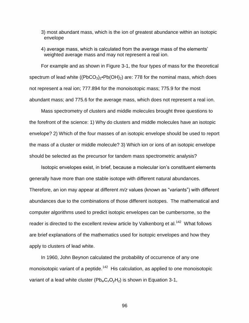
96
3) most abundant mass, which is the ion of greatest abundance within an isotopic envelope
4) average mass, which is calculated from the average mass of the elements’
weighted average mass and may not represent a real ion. For example and as shown in Figure 3-1, the four types of mass for the theoretical
spectrum of lead white ((PbCO3)2•Pb(OH)2) are: 778 for the nominal mass, which does
not represent a real ion; 777.894 for the monoisotopic mass; 775.9 for the most
abundant mass; and 775.6 for the average mass, which does not represent a real ion.
Mass spectrometry of clusters and middle molecules brought three questions to
the forefront of the science: 1) Why do clusters and middle molecules have an isotopic
envelope? 2) Which of the four masses of an isotopic envelope should be used to report
the mass of a cluster or middle molecule? 3) Which ion or ions of an isotopic envelope
should be selected as the precursor for tandem mass spectrometric analysis?
Isotopic envelopes exist, in brief, because a molecular ion’s constituent elements
generally have more than one stable isotope with different natural abundances.
Therefore, an ion may appear at different m/z values (known as “variants”) with different
abundances due to the combinations of those different isotopes. The mathematical and
computer algorithms used to predict isotopic envelopes can be cumbersome, so the
reader is directed to the excellent review article by Valkenborg et al.142 What follows
are brief explanations of the mathematics used for isotopic envelopes and how they
apply to clusters of lead white.
In 1960, John Beynon calculated the probability of occurrence of any one
monoisotopic variant of a peptide.142 His calculation, as applied to one monoisotopic
variant of a lead white cluster (PbwCxOyHz) is shown in Equation 3-1,
97
P = Pr(208Pb)w Pr(12C)x Pr(16O)y Pr(1H)z (3-1)
where P is the probability of the monoisotopic variant and Pr is the probability, given by
the percent natural abundance, of the element’s isotope. The actual number of all the
possible variants for lead white (Pb3C2O8H2) based on the total number of permutations
is actually 6,718,464 (calculated from 43223822).142,143 Though quite large, this number
incorporates all the possibilities of one isotope simply moving to a new position within
the same molecule (i.e., structural isotopomer), which would appear at the same exact
mass and thus would not be differentiated by a mass spectrometer.
So that only observable variants are considered, in 1962 Klaus Biemann
developed the stepwise procedure, which uses a particular atom’s isotopic ratios and
sums them stepwise until the molecule is accumulated.142 It is this stepwise procedure
which McLafferty referred to as “linear superposition of isotopic patterns” in his
far-reaching text.144 Yet, the stepwise procedure is laborious, practical only for very
small molecules, and relied on whole-number rounding of the ratios of isotopic
abundances.
To use exact abundances and to include middle and large molecules, in 1977
Yamamoto and McCloskey developed the polynomial expansion method.142,145
Applying this method, the isotopic envelope for a lead white cluster (PbwCxOyHz) can be
created using Equation 3-2.
(204Pb + 206Pb + 207Pb + 208Pb)w (12C + 13C)x (16O + 17O + 18O)y (1H + 2H)z
(3-2)
Each isotopic term for an element is the probability of that isotope, which is just the
natural abundance. The superscripts w, x, y, z are the count of each elements’ atom in
98
the cluster. Though a significant improvement over the stepwise method, polynomial
expansion requires significant computation because of the many possibilities (6,718,464
for lead white) and those possibilities with the same exact mass must then be
combined; once combined, the total number of possibilities will be significantly reduced
and can be calculated using combinatorial algebra to find the number of simplified
terms. For a polynomial expansion of two, three, and four terms, the respective
formulae are shown in Equation 3-3, and are already multiplied to find the total number
of simplified terms
(3-3)
where r is the power of the binomial term, s is the power of the trinomial term, and t is
the power of the quadrinomial term. The number of simplified terms for lead white using
Equation 3-3 yields 8,100 different permutations. Note that since lead white has two
elements with only two stable isotopes (C and H), the binomial term must be included
twice.
To ease the burden of computation and of combining the isobaric masses, in 1983
Yergey developed the method of multinomial expansion.142,143 Rather than collecting
identical masses as with polynomial expansion, multinomial expansion calculates
multinomial coefficients, which are equal to the frequency a variant appears in the
expansion. The equation for multinomial expansion, which is a direct corollary to
polynomial expansion, determines a variant’s probability for one element.146 Equation
3-4 shows the general form of a multinomial expansion for an element that has two
isotopic variants (e.g., C).
6
6116
2
23)1(
232 tttssr
99
(3-4)
For Equation 3-4, a and b are the abundance of the isotopic variants and n is the
number of atoms of that element in the molecule. Certainly, the left side of the Equation
is just a binomial; but, the right side of the Equation is the sum of multinomial
probability-like terms. Equation 3-5 shows the general form of a multinomial expansion
for an element that has three isotopic variants (e.g., O) and is derived as a series of
binomial expansions.146
(3-5)
For Equation 3-5, the variables from Equation 3-4 are conserved, and c is the third
isotopic variant. Similarly, Equation 3-6 shows the general form of a multinomial
expansion for an element that has four isotopic variants (e.g., Pb).
(3-6)
For Equation 3-6, the variables from Equations 3-3 and 3-4 are conserved, and d
is the fourth isotopic variant. The multinomial expansions indicated in Equations 3-4,
3-5, and 3-6 are only used to find the probability from one isotopic variant from only one
element. To obtain the probability for an entire molecule, following reassignment of the
proper variables, the probabilities for the element-specific isotopic variants must be
multiplied. For larger middle molecules, and certainly for biomolecules such as
inini
i
n baini
nba
0 )!(!
!)(
inj
j
jinjini
i
n cbjinj
ina
ini
ncba
00 )!(!
)!(
)!(!
!)(
inj
j
kjink
jink
k
jini
i
n dckjink
jinb
jinj
ina
ini
ndcba
0 00 )!(!
)!(
)!(!
)!(
)!(!
!)(
100
proteins, polynomial and multinomial expansions can result in a combinatorial explosion
and, hence, require significant amounts of computation time and memory. Therefore,
methods for the reduction of a theoretical spectrum’s complexity are employed such as
pruning of isotopic variants of low abundance and binning of isotopic variants with
differences of mass far below the resolving power of a mass spectrometer.142
Although the methods of polynomial and multinomial expansion most accurately
describe the fundamental mechanisms that create an isotopic envelope and are
sufficient for most applications, more advanced techniques and algorithms have been
introduced to mitigate the expense of computation. Most noteworthy are the methods
by Alan Rockwood, who devised aggregation of isotopic variants with the same nucleon
number and convolution by FT techniques, among others.142 Unfortunately,
Rockwood’s methods often sacrifice the infinite resolution offered by polynomial
expansion.
Finally, it should be mentioned that all of the above methods for calculating the
theoretical isotopic distribution of a molecule produce a “pattern spectrum”, that is, a
matrix of masses and their abundances. The graphical representation of a spectrum,
similar to that generated by a mass spectrometer, is achieved by applying a Gaussian
or Laplacian approximation over the pattern spectrum with a user-defined resolution.142
The second question brought about during the era of middle molecules asks which
of the four defined masses outlined above—or, more broadly applied, which of the many
masses within an isotopic envelope—should be used to report the mass of a molecular
ion. Certainly, for the majority of small-molecule mass spectrometry, only the most
abundant mass is provided, which is indeed appropriate since most elements have
101
either one isotope with a relative abundance far greater than the other isotopes (e.g., C,
N, O, H, S) or only one isotope (e.g., F, Na, P). For most small molecules the most
abundant mass is the first (lowest mass) peak in an isotopic envelope and also the
monoisotopic mass. For mass analyzers of low resolving power, this is often
indistinguishable from the nominal and average masses. Once elements containing
isotopes with relative abundances that are not dominated by the low-mass isotope (e.g.,
Cl, Br) are introduced into a small molecule, however, the most abundant mass may no
longer be the monoisotopic mass. The effect of reducing the prominence of the
monoisotopic mass is much more pronounced when elements such as lead are
introduced, whose most abundant isotope is actually the isotope of highest mass, as
shown with the following relative abundances147: 204Pb, 1.4%; 206Pb, 24.1%; 207Pb,
22.1%; 208Pb, 52.4%. Moreover, when molecules contain an increasingly large number
of a particular atom, the isotopes of low relative abundance have an increasingly large
effect on the relative abundance of the monoisotopic and most abundant mass.135,140
For example, when a hypothetical molecule composed solely of carbon reaches 92
atoms, the abundance of the 12C9113C peak is only 0.538% lower than the 12C92 peak;
when 93 carbons are reached the 12C9213C peak overtakes the 12C93 peak as it then
becomes 0.543% higher. The aforementioned effects are clearly apparent with lead
white’s molecular ion, as previously shown in Figure 3-1.
For middle- to large-mass molecules, the average mass was typically reported
prior to the advent of high resolving power instruments.139 But since the implementation
of FTICR for middle- to large-mass molecules—particularly biomolecules such as
proteins and large peptides—reporting the appropriate mass became a priority.140,141 In
102
the early days of high-resolution MS, the most abundant mass was reported; although
accurate, the actual mass may have had up to a one-Dalton error due to incorrectly
assigning contributions from heavy isotopes.140 What remains is still the monoisotopic
mass as the most reliable mass to report for middle- to large-mass molecules. But, as
noted above, as the number of atoms increase, the monoisotopic mass sharply
decreases in relative abundance. However, the monoisotopic mass as it is known
suffers from the bias in assuming that only the lowest-mass isotopes are relevant.
Indeed, the “other monoisotopic mass”—being composed of only the highest-mass
isotopes—can also be just as useful, assuming of course, that it, too, is of sufficient
abundance.148 This monoisotopic mass composed of highest-mass isotopes should be
particularly crucial to exploit for molecules containing lead since its isotopes have
unusual relative abundances. Lastly, monoisotopic masses are useful for middle- to
large-mass molecules because they do not suffer from natural isotopic variance.140,141
For instance, although the relative abundances of 12C and 13C are commonly cited as
98.93% and 1.07%, respectively, those are the “representative isotopic composition”,
which are composite values and may not represent the true abundance from any single
terrestrial source, according to the International Union of Pure and Applied Chemistry
(IUPAC).147 The isotopic abundances of 12C and 13C can actually have a range of
98.85–99.02% and 1.15–0.98%, respectively.147 So, an ion composed of only one
isotope from each of its constituent elements should not vary from among different
terrestrial samples or portions of that same sample.
The third question brought about during the era of middle molecules asks which of
the ions within an isotopic envelope should be selected as the precursor/parent ion for
103
fragmentation in MS/MS experiments. Overall, the selection of a monoisotopic peak is
preferred so that daughter ion spectra will be minimally complex and is routinely
performed on small molecules.148,149 Yet, fragmentation of non-monoisotopic peaks
may be preferable either if the monoisotopic peaks lack sufficient abundance or if
increased information about the chemical composition and structure of the precursor is
desired.149 The latter reason has been well documented in the literature with
experimental evidence141,150-156 and mathematical formulae148,149,152,153,157,158.
The information gathered from the fragmentation of non-monoisotopic peaks may
be well considered with the following two exemplar, seminal works. In 1982, McLafferty
et al. published the claim that product ions, following MS/MS of a single
non-monoisotopic ion from a precursor with a multi-isotope element, will have a different
isotopic envelope pattern than either full-scan fragments (from EI) or even the natural
abundance of the precursor’s multi-isotope element.151 Yet, the work was shown only
for small molecules with simple, two-isotope elements such Br and Cl. In 1983, Cooks
et al. expanded on McLafferty’s work by showing how a precursor can be identified from
the different isotopic patterns acquired from varying scan modes (i.e., neutral loss,
parent, and daughter) on a triple quadrupole MS.152 The claim was made that in
daughter ion spectra, fragment ions have isotopic ratios that reveal both the variant of
the parent and the number of atoms of the multi-isotopic element in the neutral
fragment. Accordingly—and critically important—if a monoisotopic variant was selected
as the parent, the daughter ion would show only as a single ion. Subsequently, from
the two works mentioned just above, several publications were spawned with both
expanded mathematical theories and applications.153-155,158
104
Lastly, fragmentation of not one ion from an isotopic envelope, but indeed, the
entire isotopic envelope itself, was surmised as a valid technique by Rockwood.148
Although he discussed that fragmentation of an envelope would lead to a complicated
spectrum, he also mentioned reasons when such a process is desired, including to
increase sensitivity for triple quadrupole-MS/MS, and when the monoisotopic peak is of
low abundance with FTICR-MS/MS. It should also be added that non-selective
precursor fragmentation also occurs in some experiments with either skimmer-cone
fragmentation29 during ESI, or with post- or in-source decay17 during matrix-assisted
laser desorption/ionization (MALDI)-ToF-MS. Considering the richness of information
from the peculiar relative abundances of the isotopes of lead, fragmentation of the entire
isotopic envelope of lead-organic clusters should prove fruitful.
The thorough historical and literature review above, regarding lead and its intimate
connection to some underlying aspects of mass spectrometry, provides the foundation
onto which the experimental results herein will be placed as capstone. Preceding
advances in analyses of lead and lead-organic clusters, theories and formulae of
isotopic distributions, and considerations of reporting and fragmentation of isotopic
envelopes, have allowed for the following results to be appreciated with greater
significance than if presented alone. What follows is a report on analysis of the artists’
pigment lead white by MALDI-LIT-MS/MS and MALDI-LIT-Orbitrap-MS/MS. Unique
clustering was observed and, following fragmentation of complete isotopic envelopes,
daughter ion spectra revealed chemical formulae for clusters that would otherwise be
difficult to elucidate. Furthermore, high-resolution and accurate mass analysis on the
Orbitrap, in conjunction with MS/MS, allowed for an alternative, complementary means
105
of cluster identification. The results have contributed to the breadth of knowledge of
organometallic clusters, isotopically complex compounds, and the tandem mass
spectrometry thereof.
Experimental Methods
Chemicals and Materials
HPLC-grade methanol (MeOH) and water were purchased from Fisher Scientific
(Fairlawn, NJ). Lead(II) carbonate basic ((PbCO3)2•Pb(OH)2), commonly referred to as
“lead white”, was purchased from Sigma Aldrich (St. Louis, MO).
Preparation of Chemicals
A slurry of lead(II) carbonate basic ((PbCO3)2•Pb(OH)2) was prepared at a
concentration of 100 μg/mL 70:30 MeOH:H2O and stored at room temperature. The
slurry was sonicated for approximately 20 minutes just prior to use.
Ionization and Instrumental Parameters
All samples were analyzed by laser desorption/ionization with an intermediate
pressure (70 mTorr) source and a N2 laser ( = 337 nm). A volume of 1 μL of sonicated
slurry was spotted on a polished stainless steel MALDI-sample plate and allowed to dry
unaided under ambient conditions. Laser parameters (i.e., laser energy and number of
laser shots) were manually tuned to obtain maximal signal, yet minimize the consequent
increase in both baseline and space charge effects. Typical laser energies were
approximately 10 μJ/pulse. The desired ionization metric of laser fluence can only be
estimated at 1.3 103 J/m2 due to the difficulty in an accurate and precise measurement
of the laser spot size, which has an approximate 100-μm spot. The number of laser
pulses for each analytical scan was controlled by the automatic gain control to maximize
the total ion signal, with fewer than 10 laser shots being typical. The sample plate was
106
moved relative to the laser via the instrument’s crystal positioning system at a rate of
one scan per spot.
Experiments were conducted using a Thermo Finnigan LTQ-XL (hereafter LTQ)
(San Jose, CA) and a Thermo Finnigan LTQ-Orbitrap (hereafter Orbitrap) (San Jose,
CA) hybrid instrument. The LTQ was used for initial experiments at relatively resolving
power and mass accuracy using both the normal (60 μs/Da) and enhanced scan rates.
The Orbitrap was used for later experiments at relatively high resolving power and mass
accuracy.
All of the aforementioned parameters for recording a full scan were kept constant
for tandem mass spectrometry. All collision-induced dissociation (CID) was conducted
in the linear ion trap of both the LTQ and Orbitrap instruments. The isolation width (W)
for all MS/MS spectra was adjusted to isolate the entire isotopic distribution of a cluster
and centered on the most abundant ion. CID parameters were manually optimized to
ensure maximal abundance from daughter cluster-ions while maintaining a relatively low
abundance of the parent cluster-ions, and are presented using the instruments’ arbitrary
unit. The W and CID values for the fragmented clusters were maintained for both LTQ
and Orbitrap experiments. The parameters for MS/MS follow, in the form (center mass,
W, CID): (430.2, 8, 30), (689.0, 8, 55), (895.0, 8, 45), (1135.0, 14, 75), (1358.0, 14, 50).
Theoretical spectra were generated with Qual Browser version 2.0.7 (Thermo
Fisher Scientific, San Jose, CA) with an output style of either “pattern”, which has
infinite resolution, or “profile”, with a full-width half-maximum (FWHM) resolution
adjusted to match that of an experimental spectrum. Automatically generated formulae
were limited to the elements Pb, C, O, and H. After contacting the manufacturer to no
107
avail, it is presumed that the model used to create theoretical spectra is proprietary
information.
Results and Discussion
The identification of ions in a complex spectrum using deductive reasoning alone
can present undue difficulties; this is certainly the case in the spectra of lead white. The
issue at the core of these difficulties is the determination of the ion, out of a broad
distribution of ions with an isotopic envelope, to be selected for the elucidation of an ion
cluster. The complementary approach of inductive reasoning alleviates these difficulties
by 1) finding the number of lead atoms to generate a matching isotopic envelope, 2)
matching daughter ion-clusters from a tandem mass spectrometric spectrum to ion
clusters in full-scan spectra, 3) exploiting patterns in the formulae of cluster ions to fill in
the gaps in the list of elucidated formulae, and 4) matching isotopic distributions
between experimentally- and theoretically-derived spectra. Finally, confirmation of
assignments of ion clusters using the superior mass accuracy of the Orbitrap was a
fail-safe arbiter among competing formulae, with few exceptions. Such an approach
was employed to identify a large number of LDI-generated cluster ions from the artists’
pigment lead white and is reported herein without any precedence in published
literature.
Full-Scan Spectra Analysis
LDI-generated spectra were recorded on an LTQ in both normal and enhanced
scan modes. The slower scan rate of the enhanced mode was used to obtain spectra
of increased mass resolution in an attempt to better identify ions. The even slower scan
rates of zoom and ultrazoom modes caused peak broadening and mass shifts from
space charge effects, and thus were not used here. An Orbitrap was ultimately used to
108
obtain superior resolution and mass accuracy. Among the different spectra, mass
assignments with the lowest error will be used to identify a cluster’s chemical formula,
with some exceptions. The spectra obtained from the LTQ and Orbitrap are in Figure
3-2. What is quite apparent is the grouping of ions into what will be termed
“superclusters”, which is analogous to the grouping observed with oligomers.
Supercluster delineation was obtained following determination of the isotopic pattern of
the most abundant ion cluster within a supercluster, which will be termed the “capital
cluster”. All clusters other than the capital cluster within a supercluster will be termed
“minuscule clusters”. For example, as seen in Figure 3-2 there are six superclusters of
nPb; six capital clusters with a most abundant ion at (rounded) m/z 208, 430, 689, 895,
1135, and 1359; and many miniscule clusters. Interestingly, the maximum abundance
of the two-lead supercluster and the decreasing relative abundances of the larger
superclusters matches the trend that was observed in the published spectra from the
LDI-generated spectra from lead carbonate159 and lead acetate131. Besides the
resolution and mass accuracy, there are no other major differences between the two
LTQ- and Orbitrap-generated spectra such as relative intensities, save for the
appearance of some low abundance miniscule clusters.
Delineation of superclusters was obtained by isotopic pattern matching of the
capital cluster to the theoretical isotopic pattern of pure Pb clusters, as shown in Figure
3-3. It is quite apparent that the unique isotopic distribution of lead (Figure 3-3, top row)
allows for rapid matching and consequent identification of the number of lead atoms in a
capital cluster (Figure 3-3, bottom row), and hence allows for the delineation of
superclusters in Figure 3-2. Also, since the heaviest isotope of lead (208Pb) has a very
109
high relative abundance (52.4%), it is readily identified and, more importantly, allows for
identification of the monoisotopic ion in clusters. Moreover, since the isotopes of the
other elements in lead white have low relative abundances (13C, 1.07%; 18O, 0.205%;
2H, 0.0115%), they have only small contribution to the monoisotopic ion of a cluster
when they are incorporated at experimental resolutions. Therefore, the monoisotopic
ion of an experimentally generated cluster can be identified by matching its relative
location within the isotopic envelope to the highest monoisotopic ion of a theoretically
derived nPb ion and will be primarily composed of 208Pb, 12C, 16O, 1H. As observed in
the bottom row of Figure 3-3, the monoisotopic ion for the superclusters are (rounded)
m/z 208, 432, 691, 898, 1139, and 1363, which contain 1, 2, 3, 4, 5, and 6 lead atoms,
respectively.
Determining the number of lead atoms in the ions of a supercluster and
subsequently determining the monoisotopic ion permits the elucidation of chemical
formulae of clusters. By selecting the monoisotopic ion, automatic formula generation
via the Qual Browser software can commence. Only formulae generated with the
lowest mass error for the normal and enhanced scan rates of the LTQ and for the
Orbitrap spectra are shown in Tables 3-1, 3-2, and 3-3. What is quite apparent is that
limiting the number of lead atoms for a cluster, which was based on supercluster
delineation, is indeed required. The most obvious example of the need to limit the
number of lead atoms is with the monoisotopic mass of 208.14 in the LTQ spectra, as
shown in Tables 3-1 and 3-2. Presumably, m/z 208.14 in the LDI spectra of lead white
results only from the Pb+ ion and not from C10O5H8+ or C13O2H20
+ as generated from
normal or enhanced scan rates, respectively. Furthermore, the need to limit Pb atoms

110
is also shown in the Orbitrap spectrum for the miniscule cluster at the monoisotopic ion
of m/z 705.92415 (Table 3-3). Again, because of supercluster delineation, the cluster
must be considered as Pb3O5H3+ and not Pb2C12O9H2
+ despite the former assignment
having a mass error three times higher than the latter. Therefore, by limiting the
software to a designated number of lead atoms for a cluster, more reliable formulae can
be generated.
The assignment of the cluster with the monoisotopic ion at m/z 705.9 is further
complicated due to lower mass errors from the LTQ with both normal (Pb3C4O2H2+,
−2.40 ppm) and enhanced (Pb3C4O2H2+, −4.60 ppm) scan rates, as compared to the
higher mass error from the Orbitrap (Pb3O5H2+, 6.463 ppm). All of the assignments
have the required number of lead atoms, but vary with the number of carbon and
oxygen atoms. Two methods were devised to reconcile this conflict: isotopic pattern
matching and inductive formula generation. The first method was that of isotopic
pattern fitting whereby experimentally and theoretically generated spectra were
compared, as shown in Figure 3-4, which has precedence in the literature131,137.
Unfortunately, spectral differences regarding either peak presence or relative
abundances are not great enough for unambiguous visual matching and, hence, the
assignment is inconclusive.
The second method, inductive formula generation, which is essentially fitting to the
trend, may be an adequate arbitrator. For instance, the formula trend within a
supercluster in Table 3-3 appears to be PbxOyHz, rather than PbxCwOyHz. Therefore, it
is proper to assign the cluster at m/z 706 as Pb3O5H2. Lastly, MS/MS provides an
additional level of confirmation, as will be later shown in the discussion.
111
The very large error (−152.240 ppm) for the miniscule cluster with the
monoisotopic ion at m/z 246.96251 in the Orbitrap spectrum indicates that the
generated formula is erroneous (Table 3-3). Considering that that ion is 22 Da higher
than the monoisotopic ion of the minuscule cluster immediately preceding it (i.e., PbOH,
m/z 224.98037) the presence of sodium (minus a hydrogen atom) was supposed. So,
one sodium atom was added to override the originally designated pool of potential
isotopes used for automatic formula generation, which resulted in the formula of PbONa
with the low error of 7.038 ppm; therefore the formula for that mass will be identified as
such. Building upon the formula of PbONa, the minuscule cluster with the monoisotopic
ion at m/z 264.7330 in the Orbitrap spectrum was also assigned to include one sodium
atom, which then makes apparent the addition of water (≈18 Da). Therefore, the ion at
m/z 264.7330 will be assigned the formula PbO2H2Na, which reduces the error from
−3.720 to 1.963.
The large errors for the clusters with the monoisotopic masses at (rounded)
m/z 208, 225, 247, 265, 432, and 449 in the LTQ spectrum (Tables 3-1 and 3-2) were
initially surprising; yet, a plausible reason for such errors of these low-m/z ions may be
that they lie outside of the calibrated range. The LTQ uses a mixture of six peptides for
normal mass range calibration: MRFA, bradykinin 1-7, bradykinin, angiotensin I,
neurotensin, and rennin substrate that have [M+H]+ ions at the monoisotopic m/z of
524.27, 757.40, 1060.7, 1296.69, 1672.92, and 1758.93, respectively; thus, a
reasonable assumption for those large errors is that the lack of a calibrant below the
m/z of MRFA. Indeed, as the experimental masses deviate from MRFA (i.e., from
m/z 449 to 208), their error concomitantly increases in an almost linear correlation.
112
Therefore, using the known exact mass of the 208Pb ion as a post-acquisition lock mass
may provide an alternative method to obtain lower errors for those low-m/z clusters; but,
this method was not tried here since the Orbitrap had already provided reliable
identifications with low error.
Tandem Mass Spectrometric Analysis
Tandem mass spectrometry was conducted on all six capital clusters with both the
LTQ at the normal scan rate and the Orbitrap, as shown in Figures 3-5 to 3-9. As
discussed in the articles by McLafferty151 and Cooks152 mentioned in the introduction,
daughter ions have a different isotopic pattern from that of their parent ion that was
individually isolated and fragmented, which stems from a daughter ion’s isotopic pattern
being derived from a combination of the isotopes included in isolation window of the
parent ion. Considering the cluster ions of lead are isotopically complex to begin with,
the entire isotopic envelope of a parent ion-cluster of lead white was selected for
fragmentation via a large isolation window. As shown in the tandem mass spectra,
using a large isolation window resulted in many daughter ion-clusters retaining their
isotopic distribution observed in the full-scan spectra.
However, some daughter ion-clusters did not retain the same isotopic distributions
observed in the full-scan spectra, which will be mentioned as they appear in the
discussion below. The most readily plausible reason for that phenomenon is from
signal attenuation of the parent cluster-ions that resulted from either the isolation or CID
steps. For instance, Reich et al. published a convincing set of experiments whereby it
was shown that the relative abundances of two daughter ions that were three Da apart,
which came from their respective parent ions of the target analyte and the tri-deuterated
form of that analyte, varied as a function of the isolation width used prior to CID of the
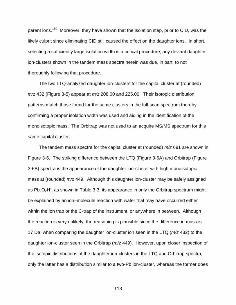
113
parent ions.160 Moreover, they have shown that the isolation step, prior to CID, was the
likely culprit since eliminating CID still caused the effect on the daughter ions. In short,
selecting a sufficiently large isolation width is a critical procedure; any deviant daughter
ion-clusters shown in the tandem mass spectra herein was due, in part, to not
thoroughly following that procedure.
The two LTQ-analyzed daughter ion-clusters for the capital cluster at (rounded)
m/z 432 (Figure 3-5) appear at m/z 208.00 and 225.00. Their isotopic distribution
patterns match those found for the same clusters in the full-scan spectrum thereby
confirming a proper isolation width was used and aiding in the identification of the
monoisotopic mass. The Orbitrap was not used to an acquire MS/MS spectrum for this
same capital cluster.
The tandem mass spectra for the capital cluster at (rounded) m/z 691 are shown in
Figure 3-6. The striking difference between the LTQ (Figure 3-6A) and Orbitrap (Figure
3-6B) spectra is the appearance of the daughter ion-cluster with high monoisotopic
mass at (rounded) m/z 449. Although this daughter ion-cluster may be safely assigned
as Pb2O2H+
, as shown in Table 3-3, its appearance in only the Orbitrap spectrum might
be explained by an ion–molecule reaction with water that may have occurred either
within the ion trap or the C-trap of the instrument, or anywhere in between. Although
the reaction is very unlikely, the reasoning is plausible since the difference in mass is
17 Da, when comparing the daughter ion-cluster ion seen in the LTQ (m/z 432) to the
daughter ion-cluster seen in the Orbitrap (m/z 449). However, upon closer inspection of
the isotopic distributions of the daughter ion-clusters in the LTQ and Orbitrap spectra,
only the latter has a distribution similar to a two-Pb ion-cluster, whereas the former does
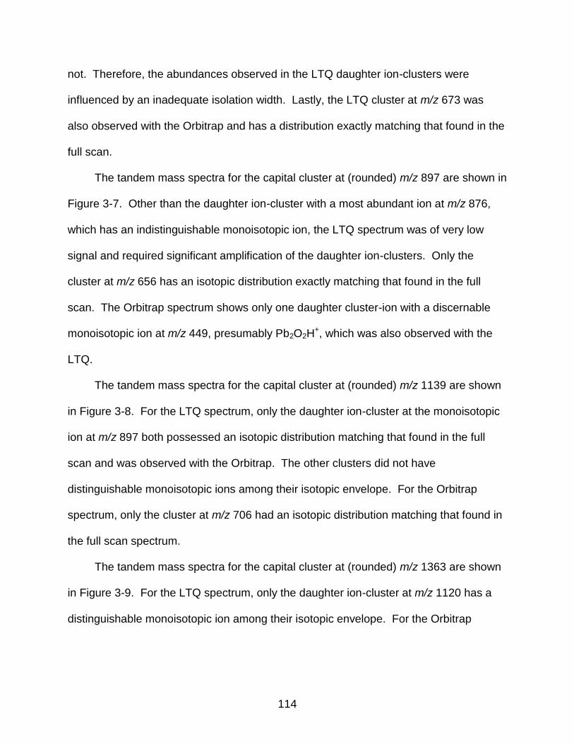
114
not. Therefore, the abundances observed in the LTQ daughter ion-clusters were
influenced by an inadequate isolation width. Lastly, the LTQ cluster at m/z 673 was
also observed with the Orbitrap and has a distribution exactly matching that found in the
full scan.
The tandem mass spectra for the capital cluster at (rounded) m/z 897 are shown in
Figure 3-7. Other than the daughter ion-cluster with a most abundant ion at m/z 876,
which has an indistinguishable monoisotopic ion, the LTQ spectrum was of very low
signal and required significant amplification of the daughter ion-clusters. Only the
cluster at m/z 656 has an isotopic distribution exactly matching that found in the full
scan. The Orbitrap spectrum shows only one daughter cluster-ion with a discernable
monoisotopic ion at m/z 449, presumably Pb2O2H+, which was also observed with the
LTQ.
The tandem mass spectra for the capital cluster at (rounded) m/z 1139 are shown
in Figure 3-8. For the LTQ spectrum, only the daughter ion-cluster at the monoisotopic
ion at m/z 897 both possessed an isotopic distribution matching that found in the full
scan and was observed with the Orbitrap. The other clusters did not have
distinguishable monoisotopic ions among their isotopic envelope. For the Orbitrap
spectrum, only the cluster at m/z 706 had an isotopic distribution matching that found in
the full scan spectrum.
The tandem mass spectra for the capital cluster at (rounded) m/z 1363 are shown
in Figure 3-9. For the LTQ spectrum, only the daughter ion-cluster at m/z 1120 has a
distinguishable monoisotopic ion among their isotopic envelope. For the Orbitrap
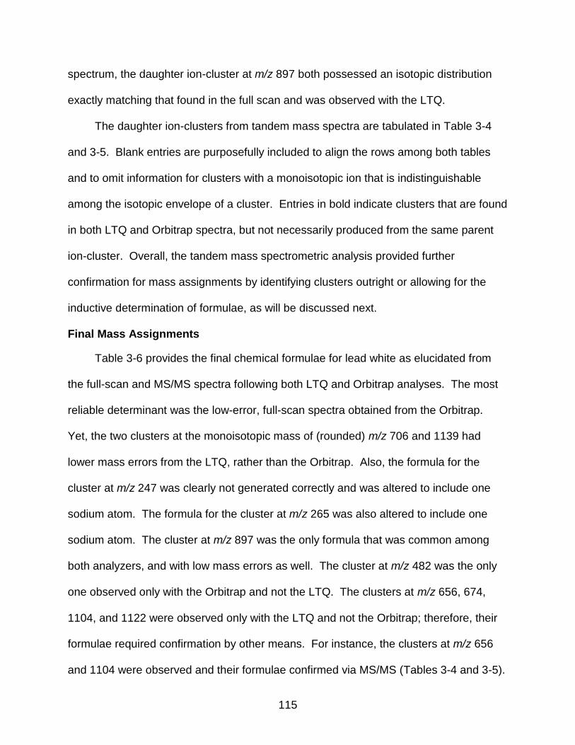
115
spectrum, the daughter ion-cluster at m/z 897 both possessed an isotopic distribution
exactly matching that found in the full scan and was observed with the LTQ.
The daughter ion-clusters from tandem mass spectra are tabulated in Table 3-4
and 3-5. Blank entries are purposefully included to align the rows among both tables
and to omit information for clusters with a monoisotopic ion that is indistinguishable
among the isotopic envelope of a cluster. Entries in bold indicate clusters that are found
in both LTQ and Orbitrap spectra, but not necessarily produced from the same parent
ion-cluster. Overall, the tandem mass spectrometric analysis provided further
confirmation for mass assignments by identifying clusters outright or allowing for the
inductive determination of formulae, as will be discussed next.
Final Mass Assignments
Table 3-6 provides the final chemical formulae for lead white as elucidated from
the full-scan and MS/MS spectra following both LTQ and Orbitrap analyses. The most
reliable determinant was the low-error, full-scan spectra obtained from the Orbitrap.
Yet, the two clusters at the monoisotopic mass of (rounded) m/z 706 and 1139 had
lower mass errors from the LTQ, rather than the Orbitrap. Also, the formula for the
cluster at m/z 247 was clearly not generated correctly and was altered to include one
sodium atom. The formula for the cluster at m/z 265 was also altered to include one
sodium atom. The cluster at m/z 897 was the only formula that was common among
both analyzers, and with low mass errors as well. The cluster at m/z 482 was the only
one observed only with the Orbitrap and not the LTQ. The clusters at m/z 656, 674,
1104, and 1122 were observed only with the LTQ and not the Orbitrap; therefore, their
formulae required confirmation by other means. For instance, the clusters at m/z 656
and 1104 were observed and their formulae confirmed via MS/MS (Tables 3-4 and 3-5).
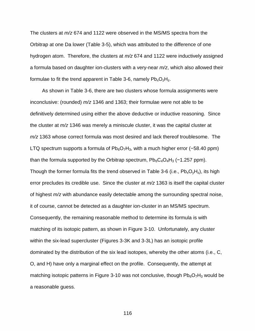
116
The clusters at m/z 674 and 1122 were observed in the MS/MS spectra from the
Orbitrap at one Da lower (Table 3-5), which was attributed to the difference of one
hydrogen atom. Therefore, the clusters at m/z 674 and 1122 were inductively assigned
a formula based on daughter ion-clusters with a very-near m/z, which also allowed their
formulae to fit the trend apparent in Table 3-6, namely PbxOzHz.
As shown in Table 3-6, there are two clusters whose formula assignments were
inconclusive: (rounded) m/z 1346 and 1363; their formulae were not able to be
definitively determined using either the above deductive or inductive reasoning. Since
the cluster at m/z 1346 was merely a miniscule cluster, it was the capital cluster at
m/z 1363 whose correct formula was most desired and lack thereof troublesome. The
LTQ spectrum supports a formula of Pb6O7H3, with a much higher error (−58.40 ppm)
than the formula supported by the Orbitrap spectrum, Pb6C4O4H3 (−1.257 ppm).
Though the former formula fits the trend observed in Table 3-6 (i.e., PbxOyHz), its high
error precludes its credible use. Since the cluster at m/z 1363 is itself the capital cluster
of highest m/z with abundance easily detectable among the surrounding spectral noise,
it of course, cannot be detected as a daughter ion-cluster in an MS/MS spectrum.
Consequently, the remaining reasonable method to determine its formula is with
matching of its isotopic pattern, as shown in Figure 3-10. Unfortunately, any cluster
within the six-lead supercluster (Figures 3-3K and 3-3L) has an isotopic profile
dominated by the distribution of the six lead isotopes, whereby the other atoms (i.e., C,
O, and H) have only a marginal effect on the profile. Consequently, the attempt at
matching isotopic patterns in Figure 3-10 was not conclusive, though Pb6O7H3 would be
a reasonable guess.
117
Final mass assignments were in the form PbxOyHz with the inclusion of sodium for
two low-mass clusters. The reason for the exclusion of integer clusters of Pbn larger
than Pb1 was not immediately apparent from the data, but high laser energy might have
been a cause161. Furthermore, high laser energy may have also contributed to the
exclusion of carbon. Experiments with the LDI-generated clusters of Os3(CO)12 resulted
in an increasing loss of carbonyl groups following a rise in laser power.161 As
mentioned in the introduction, carbon was included in clusters of lead acetate generated
by CI127 and LDI131, which was contained mostly within the acetate moiety, but was
excluded from LDI-generated clusters of lead carbonate123. Lastly, loss of carbon, in
the form of carbonyl, was observed and extensively discussed with the LDI-generated
clusters of Rh6(CO)16.134 Thus, the omission of carbon from the final mass assignments
are not necessarily cause for immediate concern.
Conclusion
For the first time, the LDI-generated, LTQ- and Orbitrap-analyzed full-scan and
tandem mass spectra of the artists’ pigment lead white have been reported. Direct
experimental evidence combined with a variety of deductive and inductive reasoning
allowed for the near-complete elucidation of the peculiar mass spectrum of lead white,
which was composed of numerous cluster ions with both relatively complex isotopic
distributions and wide isotopic envelopes. Mass assignments appeared to fit a general
pattern of PbxOyHz with the exclusion of both carbon and integer clusters of Pbn larger
than Pb1.
Key to the successful assignments of formulae was the multi-step method used
herein. The initial and most critical step was to determine the number of lead atoms of
a cluster that allowed for both the identification of the monoisotopic ion and a limitation
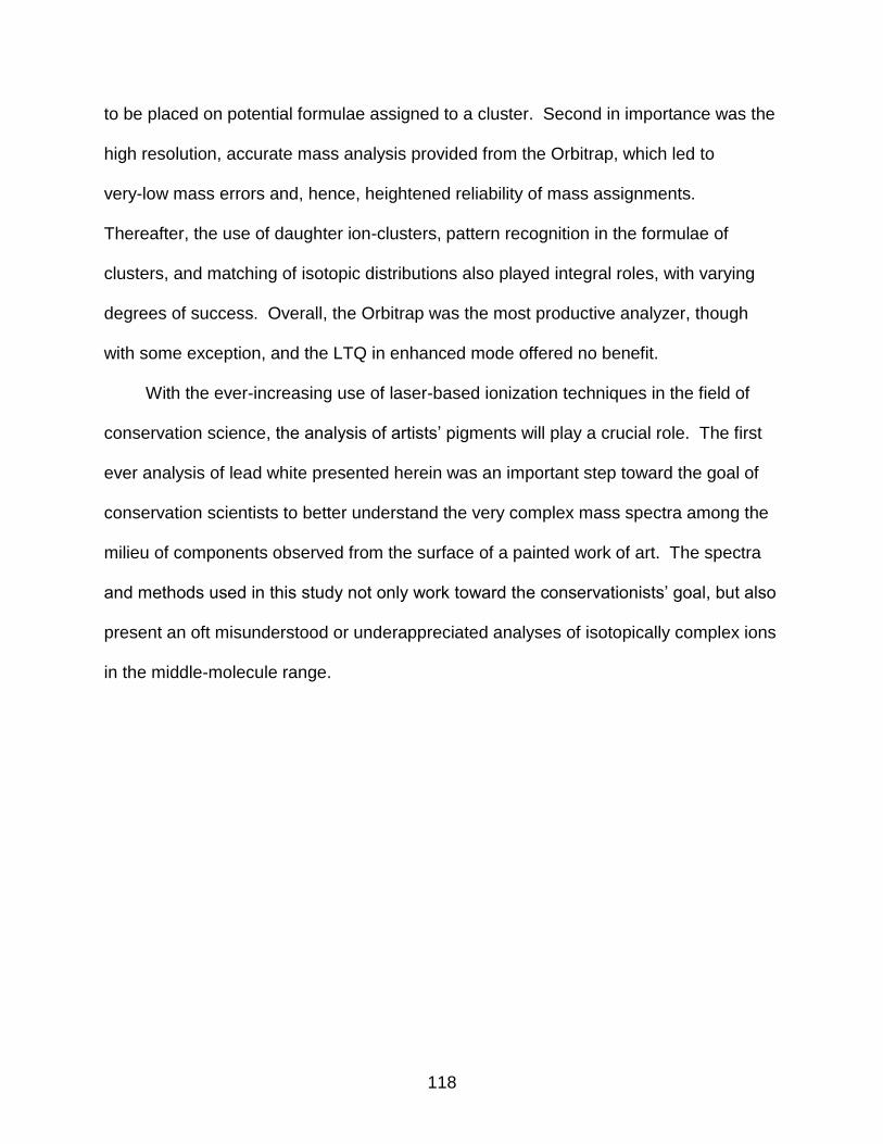
118
to be placed on potential formulae assigned to a cluster. Second in importance was the
high resolution, accurate mass analysis provided from the Orbitrap, which led to
very-low mass errors and, hence, heightened reliability of mass assignments.
Thereafter, the use of daughter ion-clusters, pattern recognition in the formulae of
clusters, and matching of isotopic distributions also played integral roles, with varying
degrees of success. Overall, the Orbitrap was the most productive analyzer, though
with some exception, and the LTQ in enhanced mode offered no benefit.
With the ever-increasing use of laser-based ionization techniques in the field of
conservation science, the analysis of artists’ pigments will play a crucial role. The first
ever analysis of lead white presented herein was an important step toward the goal of
conservation scientists to better understand the very complex mass spectra among the
milieu of components observed from the surface of a painted work of art. The spectra
and methods used in this study not only work toward the conservationists’ goal, but also
present an oft misunderstood or underappreciated analyses of isotopically complex ions
in the middle-molecule range.
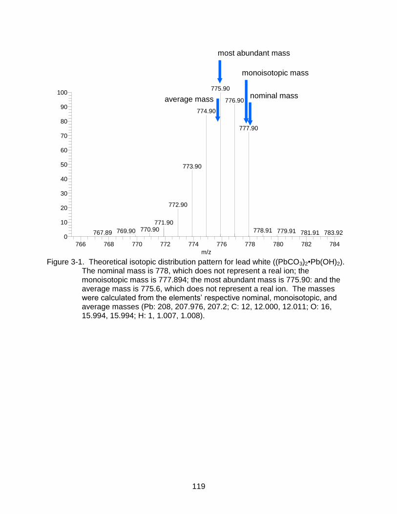
119
Figure 3-1. Theoretical isotopic distribution pattern for lead white ((PbCO3)2•Pb(OH)2). The nominal mass is 778, which does not represent a real ion; the monoisotopic mass is 777.894; the most abundant mass is 775.90: and the average mass is 775.6, which does not represent a real ion. The masses were calculated from the elements’ respective nominal, monoisotopic, and average masses (Pb: 208, 207.976, 207.2; C: 12, 12.000, 12.011; O: 16, 15.994, 15.994; H: 1, 1.007, 1.008).
Pb3C2O8H2: Pb3 C2 O8 H2 pa Chrg 1
766 768 770 772 774 776 778 780 782 784
m/z
0
10
20
30
40
50
60
70
80
90
100
Re
lative
Abu
nd
an
ce
775.90
776.90
774.90
777.90
773.90
772.90
771.90770.90 778.91769.90 779.91767.89 781.91 783.92
most abundant mass
nominal mass
monoisotopic mass
average mass
120
Figure 3-2. LDI-generated, full-scan, positive-mode spectrum of lead white analyzed by LTQ with normal (A) and enhanced (B) scan rates and Orbitrap (C). Lead atom-counts are bracketed into superclusters.
1Pb 2Pb 3Pb 4Pb 5Pb 6Pb
MS_Undil_Pb_L15_E2 #1-17 RT: 0.00-0.71 AV: 17 NL: 9.14E6T: FTMS + p MALDI Full ms [50.00-2000.00]
200 300 400 500 600 700 800 900 1000 1100 1200 1300 1400
m/z
0
20
40
60
80
100
Re
lative
Ab
un
da
nce
429.94844
464.96185688.93537
894.89812
912.90868224.98034 481.951031134.88069634.35137246.96251 1358.85293
927.89554536.98380359.98979
Pb10x_enhanced_J1 #1-50 RT: 0.00-0.75 AV: 50 NL: 9.45E4T: ITMS + p MALDI E Full ms [100.00-2000.00]
200 300 400 500 600 700 800 900 1000 1100 1200 1300 1400
m/z
0
20
40
60
80
100
Re
lative
Ab
un
da
nce
430.12
447.12688.96 894.88
208.28
689.96 895.88671.96465.08
896.881134.80225.24 653.96 703.92414.12 897.88566.04361.16 1358.841117.80806.92 982.92507.04 1151.80 1252.84
Pb10x_normal_J1 #1-50 RT: 0.00-0.38 AV: 50 NL: 1.73E5T: ITMS + p MALDI Full ms [100.00-2000.00]
200 300 400 500 600 700 800 900 1000 1100 1200 1300 1400
m/z
0
20
40
60
80
100
Re
lative
Ab
un
da
nce
430.08
689.00447.08 894.92
208.17
672.00 690.00895.92465.08
1134.83896.92
704.00225.17 913.83654.00 1358.751117.83 1150.75414.08 601.00362.17265.17 807.00507.08 731.17 1030.92930.83 1253.83
B
C
A
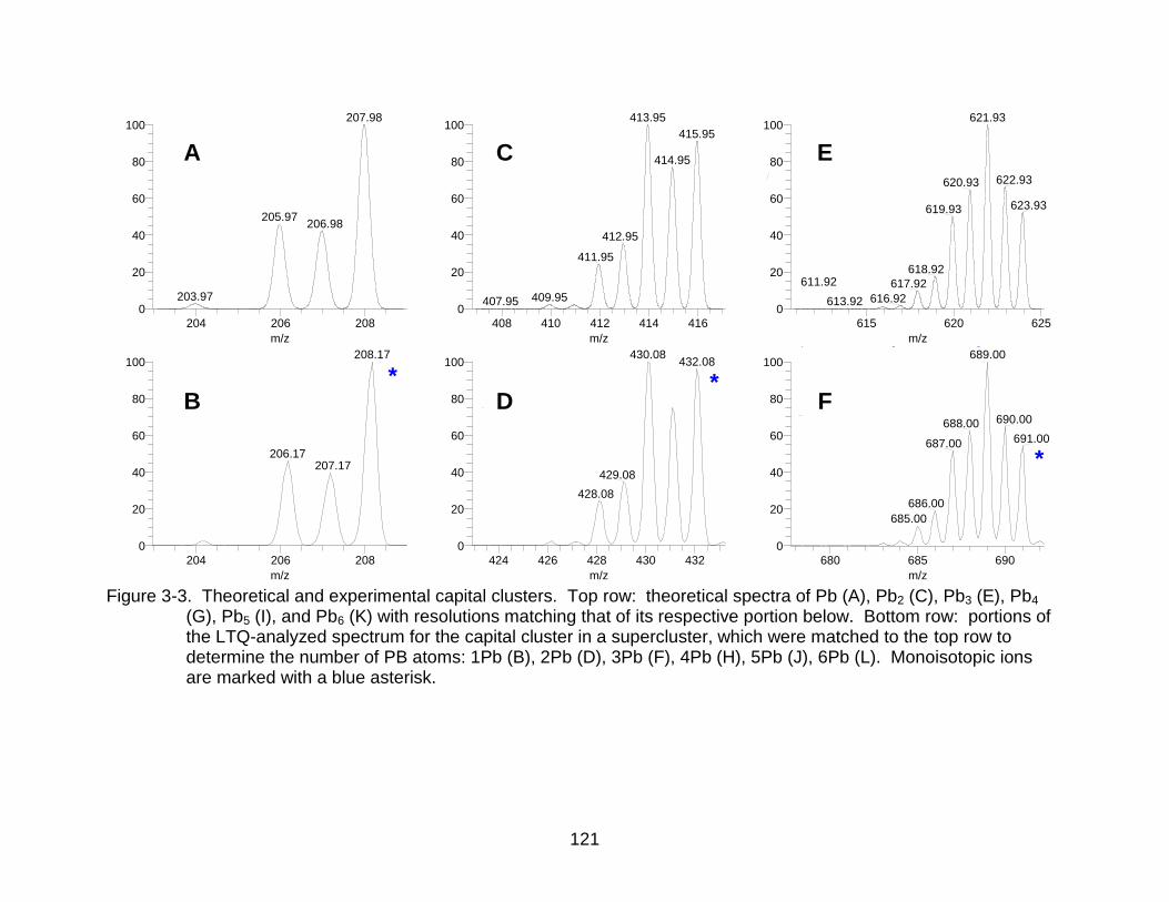
121
Figure 3-3. Theoretical and experimental capital clusters. Top row: theoretical spectra of Pb (A), Pb2 (C), Pb3 (E), Pb4 (G), Pb5 (I), and Pb6 (K) with resolutions matching that of its respective portion below. Bottom row: portions of the LTQ-analyzed spectrum for the capital cluster in a supercluster, which were matched to the top row to determine the number of PB atoms: 1Pb (B), 2Pb (D), 3Pb (F), 4Pb (H), 5Pb (J), 6Pb (L). Monoisotopic ions are marked with a blue asterisk.
Pb: Pb1 p(gss, s/p:40) Chrg 1R: 669 Res.Pwr. @FWHM
204 206 208
m/z
0
20
40
60
80
100
Re
lative
Ab
un
da
nce
207.98
205.97206.98
203.97
Pb10x_normal_J1 #1-50 RT: 0.00-0.38 AV: 50 NL:T: ITMS + p MALDI Full ms [100.00-2000.00]
204 206 208
m/z
0
20
40
60
80
100
Re
lative
Ab
un
da
nce
208.17
206.17207.17
Pb10x_normal_J1 #1-50 RT: 0.00-0.38 AV: 50 NL:T: ITMS + p MALDI Full ms [100.00-2000.00]
424 426 428 430 432
m/z
0
20
40
60
80
100
Re
lative
Ab
un
da
nce
430.08432.08
429.08
428.08
Pb2: Pb2 p(gss, s/p:40) Chrg 1R: 1196 Res.Pwr. @FWHM
408 410 412 414 416
m/z
0
20
40
60
80
100
Re
lative
Ab
un
da
nce
413.95
415.95
414.95
412.95
411.95
409.95407.95
Pb10x_normal_J1 #1-50 RT: 0.00-0.38 AV: 50 NL:T: ITMS + p MALDI Full ms [100.00-2000.00]
680 685 690
m/z
0
20
40
60
80
100
Re
lative
Ab
un
da
nce
689.00
690.00688.00
691.00687.00
686.00
685.00
Pb3: Pb3 p(gss, s/p:40) Chrg 1R: 1750 Res.Pwr. @FWHM
615 620 625
m/z
0
20
40
60
80
100
Re
lative
Ab
un
da
nce
621.93
622.93620.93
623.93619.93
618.92
617.92
616.92613.92
611.92
A
B
C
D
E
F * *
*
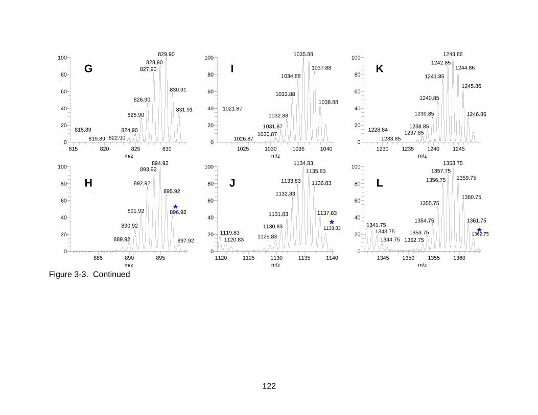
122
Figure 3-3. Continued
Pb6: Pb6 p(gss, s/p:40) Chrg 1R: 3231 Res.Pwr. @FWHM
1230 1235 1240 1245
m/z
0
20
40
60
80
100
Re
lative
Ab
un
da
nce
1243.86
1242.851244.86
1241.85
1245.86
1240.85
1239.85 1246.86
1238.851237.85
1233.85
1228.84
Pb10x_normal_J1 #1-50 RT: 0.00-0.38 AV: 50 NL:T: ITMS + p MALDI Full ms [100.00-2000.00]
1345 1350 1355 1360
m/z
0
20
40
60
80
100
Re
lative
Ab
un
da
nce
1358.75
1357.75
1359.751356.75
1360.751355.75
1361.751354.751341.75
1343.75 1353.75
1344.75 1352.75
Pb10x_normal_J1 #1-50 RT: 0.00-0.38 AV: 50 NL:T: ITMS + p MALDI Full ms [100.00-2000.00]
1120 1125 1130 1135 1140
m/z
0
20
40
60
80
100
Re
lative
Ab
un
da
nce
1134.83
1135.83
1133.83 1136.83
1132.83
1137.831131.83
1130.831119.83
1129.831120.83
Pb5: Pb5 p(gss, s/p:40) Chrg 1R: 2544 Res.Pwr. @FWHM
1025 1030 1035 1040
m/z
0
20
40
60
80
100
Rela
tive A
bundance
1035.88
1037.88
1034.88
1033.88
1038.88
1032.88
1031.87
1030.871026.87
1021.87
Pb4: Pb4 p(gss, s/p:40) Chrg 1R: 2270 Res.Pwr. @FWHM
815 820 825 830
m/z
0
20
40
60
80
100
Re
lative
Ab
un
da
nce
829.90
828.90
827.90
830.91
826.90
831.91825.90
824.90
822.90819.89
815.89
Pb10x_normal_J1 #1-50 RT: 0.00-0.38 AV: 50 NL:T: ITMS + p MALDI Full ms [100.00-2000.00]
885 890 895
m/z
0
20
40
60
80
100
Re
lative
Ab
un
da
nce
894.92893.92
892.92
895.92
891.92 896.92
890.92
889.92 897.92
G
H
I
J
K
L
* 1138.83
*
* 1362.75
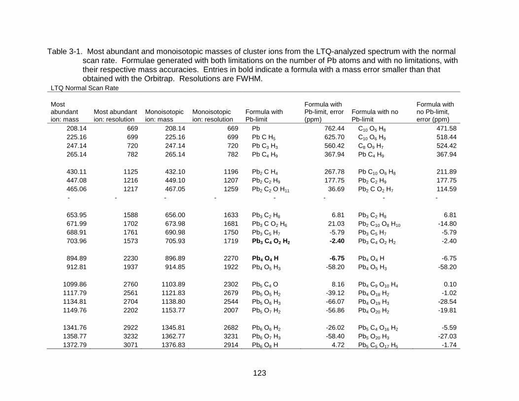
123
Table 3-1. Most abundant and monoisotopic masses of cluster ions from the LTQ-analyzed spectrum with the normal scan rate. Formulae generated with both limitations on the number of Pb atoms and with no limitations, with their respective mass accuracies. Entries in bold indicate a formula with a mass error smaller than that obtained with the Orbitrap. Resolutions are FWHM.
LTQ Normal Scan Rate
Most abundant ion: mass
Most abundant ion: resolution
Monoisotopic ion: mass
Monoisotopic ion: resolution
Formula with Pb-limit
Formula with Pb-limit, error (ppm)
Formula with no Pb-limit
Formula with no Pb-limit, error (ppm)
208.14 669 208.14 669 Pb 762.44 C10 O5 H8 471.58
225.16 699 225.16 699 Pb C H5 625.70 C10 O6 H9 518.44
247.14 720 247.14 720 Pb C3 H3 560.42 C8 O9 H7 524.42
265.14 782 265.14 782 Pb C4 H9 367.94 Pb C4 H9 367.94
430.11 1125 432.10 1196 Pb2 C H4 267.78 Pb C10 O6 H8 211.89
447.08 1216 449.10 1207 Pb2 C2 H9 177.75 Pb2 C2 H9 177.75
465.06 1217 467.05 1259 Pb2 C2 O H11 36.69 Pb2 C O2 H7 114.59
- - - - - - - -
653.95 1588 656.00 1633 Pb3 C2 H8 6.81 Pb3 C2 H8 6.81
671.99 1702 673.98 1681 Pb3 C O2 H6 21.03 Pb2 C10 O8 H10 -14.80
688.91 1761 690.98 1750 Pb3 C5 H7 -5.79 Pb3 C5 H7 -5.79
703.96 1573 705.93 1719 Pb3 C4 O2 H2 -2.40 Pb3 C4 O2 H2 -2.40
894.89 2230 896.89 2270 Pb4 O4 H -6.75 Pb4 O4 H -6.75
912.81 1937 914.85 1922 Pb4 O5 H3 -58.20 Pb4 O5 H3 -58.20
1099.86 2760 1103.89 2302 Pb5 C4 O 8.16 Pb4 C9 O10 H4 0.10
1117.79 2561 1121.83 2679 Pb5 O5 H2 -39.12 Pb4 O18 H2 -1.02
1134.81 2704 1138.80 2544 Pb5 O6 H3 -66.07 Pb4 O19 H3 -28.54
1149.76 2202 1153.77 2007 Pb5 O7 H2 -56.86 Pb4 O20 H2 -19.81
1341.76 2922 1345.81 2682 Pb6 O6 H2 -26.02 Pb5 C4 O16 H2 -5.59
1358.77 3232 1362.77 3231 Pb6 O7 H3 -58.40 Pb5 O20 H3 -27.03
1372.79 3071 1376.83 2914 Pb6 O8 H 4.72 Pb5 C5 O17 H5 -1.74
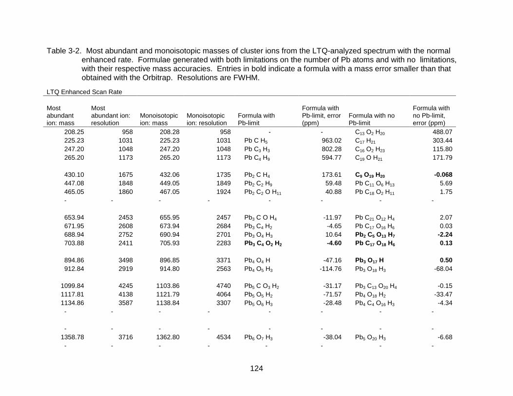
124
Table 3-2. Most abundant and monoisotopic masses of cluster ions from the LTQ-analyzed spectrum with the normal enhanced rate. Formulae generated with both limitations on the number of Pb atoms and with no limitations, with their respective mass accuracies. Entries in bold indicate a formula with a mass error smaller than that obtained with the Orbitrap. Resolutions are FWHM.
LTQ Enhanced Scan Rate
Most abundant ion: mass
Most abundant ion: resolution
Monoisotopic ion: mass
Monoisotopic ion: resolution
Formula with Pb-limit
Formula with Pb-limit, error (ppm)
Formula with no Pb-limit
Formula with no Pb-limit, error (ppm)
208.25 958 208.28 958 - - C13 O2 H20 488.07
225.23 1031 225.23 1031 Pb C H5 963.02 C17 H21 303.44
247.20 1048 247.20 1048 Pb C3 H3 802.28 C16 O2 H23 115.80
265.20 1173 265.20 1173 Pb C4 H9 594.77 C19 O H21 171.79
430.10 1675 432.06 1735 Pb2 C H4 173.61 C9 O19 H20 -0.068
447.08 1848 449.05 1849 Pb2 C2 H9 59.48 Pb C11 O6 H13 5.69
465.05 1860 467.05 1924 Pb2 C2 O H11 40.88 Pb C18 O2 H11 1.75
- - - - - - - -
653.94 2453 655.95 2457 Pb3 C O H4 -11.97 Pb C21 O12 H4 2.07
671.95 2608 673.94 2684 Pb3 C4 H2 -4.65 Pb C17 O16 H6 0.03
688.94 2752 690.94 2701 Pb3 O4 H3 10.64 Pb2 C5 O13 H7 -2.24
703.88 2411 705.93 2283 Pb3 C4 O2 H2 -4.60 Pb C17 O18 H6 0.13
894.86 3498 896.85 3371 Pb4 O4 H -47.16 Pb3 O17 H 0.50
912.84 2919 914.80 2563 Pb4 O5 H3 -114.76 Pb3 O18 H3 -68.04
1099.84 4245 1103.86 4740 Pb5 C O3 H2 -31.17 Pb3 C13 O20 H4 -0.15
1117.81 4138 1121.79 4064 Pb5 O5 H2 -71.57 Pb4 O18 H2 -33.47
1134.86 3587 1138.84 3307 Pb5 O6 H3 -28.48 Pb4 C4 O16 H3 -4.34
- - - - - - - -
- - - - - - - -
1358.78 3716 1362.80 4534 Pb6 O7 H3 -38.04 Pb5 O20 H3 -6.68
- - - - - - - -
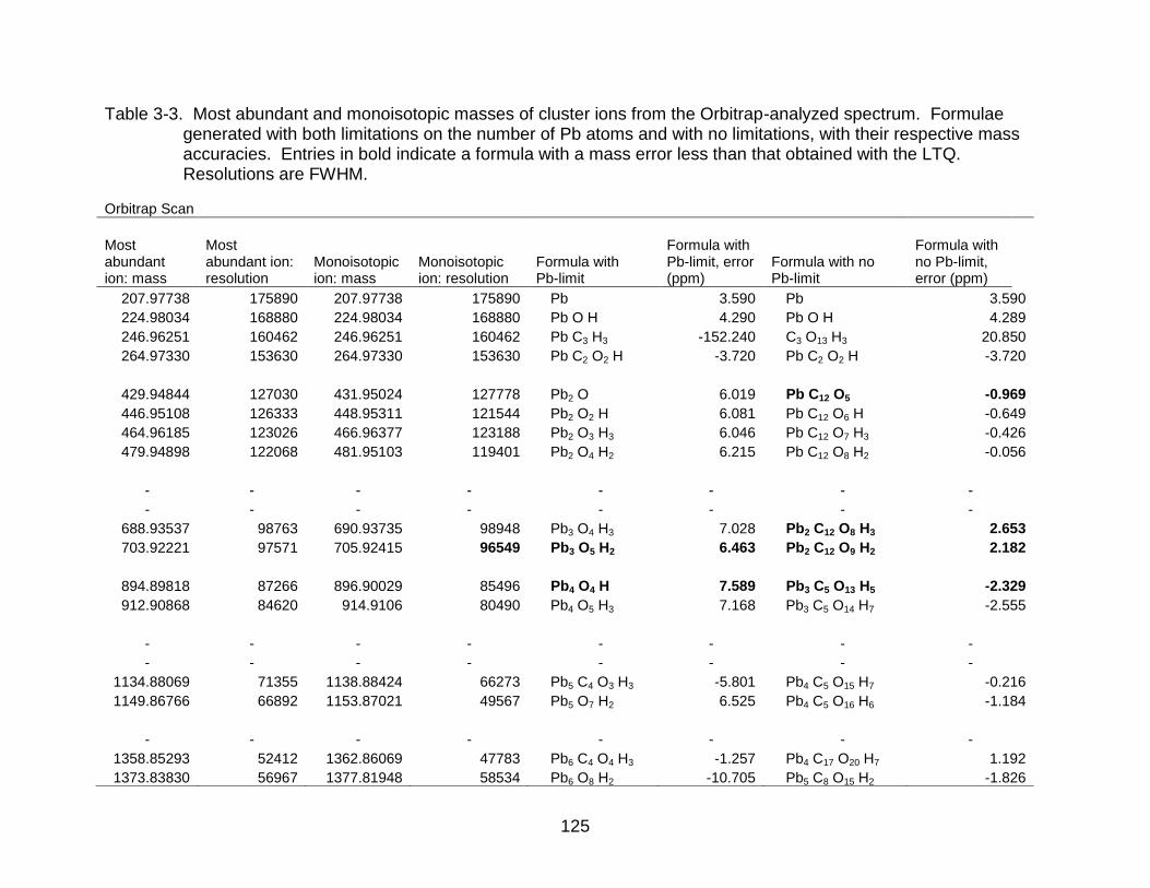
125
Table 3-3. Most abundant and monoisotopic masses of cluster ions from the Orbitrap-analyzed spectrum. Formulae generated with both limitations on the number of Pb atoms and with no limitations, with their respective mass accuracies. Entries in bold indicate a formula with a mass error less than that obtained with the LTQ. Resolutions are FWHM.
Orbitrap Scan
Most abundant ion: mass
Most abundant ion: resolution
Monoisotopic ion: mass
Monoisotopic ion: resolution
Formula with Pb-limit
Formula with Pb-limit, error (ppm)
Formula with no Pb-limit
Formula with no Pb-limit, error (ppm)
207.97738 175890 207.97738 175890 Pb 3.590 Pb 3.590
224.98034 168880 224.98034 168880 Pb O H 4.290 Pb O H 4.289
246.96251 160462 246.96251 160462 Pb C3 H3 -152.240 C3 O13 H3 20.850
264.97330 153630 264.97330 153630 Pb C2 O2 H -3.720 Pb C2 O2 H -3.720
429.94844 127030 431.95024 127778 Pb2 O 6.019 Pb C12 O5 -0.969
446.95108 126333 448.95311 121544 Pb2 O2 H 6.081 Pb C12 O6 H -0.649
464.96185 123026 466.96377 123188 Pb2 O3 H3 6.046 Pb C12 O7 H3 -0.426
479.94898 122068 481.95103 119401 Pb2 O4 H2 6.215 Pb C12 O8 H2 -0.056
- - - - - - - -
- - - - - - - -
688.93537 98763 690.93735 98948 Pb3 O4 H3 7.028 Pb2 C12 O8 H3 2.653
703.92221 97571 705.92415 96549 Pb3 O5 H2 6.463 Pb2 C12 O9 H2 2.182
894.89818 87266 896.90029 85496 Pb4 O4 H 7.589 Pb3 C5 O13 H5 -2.329
912.90868 84620 914.9106 80490 Pb4 O5 H3 7.168 Pb3 C5 O14 H7 -2.555
- - - - - - - -
- - - - - - - -
1134.88069 71355 1138.88424 66273 Pb5 C4 O3 H3 -5.801 Pb4 C5 O15 H7 -0.216
1149.86766 66892 1153.87021 49567 Pb5 O7 H2 6.525 Pb4 C5 O16 H6 -1.184
- - - - - - - -
1358.85293 52412 1362.86069 47783 Pb6 C4 O4 H3 -1.257 Pb4 C17 O20 H7 1.192
1373.83830 56967 1377.81948 58534 Pb6 O8 H2 -10.705 Pb5 C8 O15 H2 -1.826
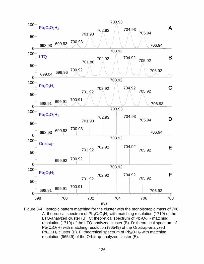
126
Figure 3-4. Isotopic pattern matching for the cluster with the monoisotopic mass of 706. A: theoretical spectrum of Pb3C4O2H2 with matching resolution (1719) of the LTQ-analyzed cluster (B). C: theoretical spectrum of Pb3O5H2 matching resolution (1719) of the LTQ-analyzed cluster (B). D: theoretical spectrum of Pb3C4O2H2 with matching resolution (96549) of the Orbitrap-analyzed Pb3O5H2 cluster (B). F: theoretical spectrum of Pb3O5H2 with matching resolution (96549) of the Orbitrap-analyzed cluster (E).
698 700 702 704 706 708
m/z
0
50
100
0
50
100
0
50
100
0
50
100
Rela
tive A
bundance 0
50
100
0
50
100703.93
704.93702.93705.94701.93
700.93699.93 706.94698.93
703.92
704.92702.92705.92701.88
700.92 706.92699.96699.04
703.92
704.92702.92705.92701.92
700.91699.91698.91 706.93
703.93
704.93702.93705.94701.93
700.93699.93 706.94698.93
703.92
704.92702.92701.92 705.92
700.92699.92
703.92
704.92702.92705.92701.92
700.91699.91
698.91 706.92
NL:6.35E3
Pb 3 C 4 O 2 H 2: Pb 3 C 4 O 2 H 2
p (gss, s /p:40) Chrg 1R: 1719 Res .Pwr . @FWHM
NL:8.47E3
Pb10x_enhanced_J1#1-50 RT: 0.00-0.75 AV: 50 T: ITMS + p MALDI E Full ms [100.00-2000.00]
NL:6.42E3
Pb 3 O 5 H 2: Pb 3 O 5 H 2
p (gss, s /p:40) Chrg 1R: 1719 Res .Pwr . @FWHM
NL:6.26E3
Pb 3 C 4 O 2 H 2: Pb 3 C 4 O 2 H 2
p (gss, s /p:40) Chrg 1R: 96549 Res .Pwr . @FWHM
NL:3.80E6
ms_undil_pb_l15_e2#1-17 RT: 0.00-0.71 AV: 17 T: FTMS + p MALDI Full ms [50.00-2000.00]
NL:6.38E3
Pb 3 O 5 H 2: Pb 3 O 5 H 2
p (gss, s /p:40) Chrg 1R: 96549 Res .Pwr . @FWHM
A
B
C
D
E
F
Pb3C4O2H2
LTQ
Pb3O5H2
Pb3C4O2H2
Orbitrap
Pb3O5H2
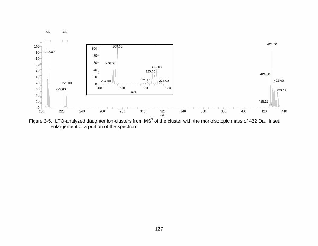
127
Figure 3-5. LTQ-analyzed daughter ion-clusters from MS2 of the cluster with the monoisotopic mass of 432 Da. Inset: enlargement of a portion of the spectrum
x20 PbBasic_MS2_430_wide_J7 #1-100 RT: 0.00-1.62 AV: 100 NL: 1.41E4T: ITMS + p MALDI Full ms2 [email protected] [115.00-450.00]
200 220 240 260 280 300 320 340 360 380 400 420 440
m/z
0
10
20
30
40
50
60
70
80
90
100
Re
lative
Ab
un
da
nce
428.00
426.00
429.00
433.17
425.17
208.00
225.00
223.00
PbBasic_MS2_430_wide_J7 #1-100 RT: 0.00-1.62 AV:T: ITMS + p MALDI Full ms2 [email protected] [115.00-4 ...
200 210 220 230
m/z
0
20
40
60
80
100R
ela
tive
Ab
un
da
nce
208.00
206.00
225.00
223.00
221.17 226.08204.00
x20
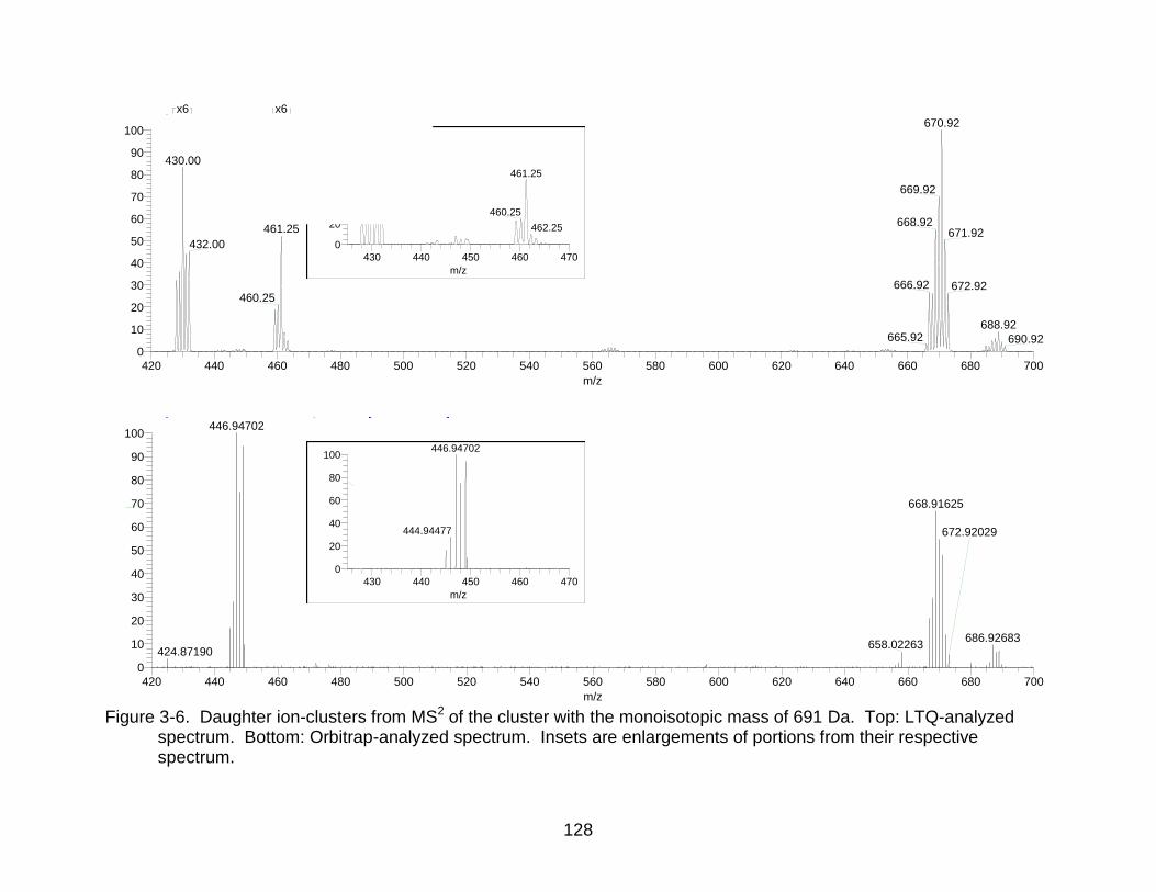
128
Figure 3-6. Daughter ion-clusters from MS2 of the cluster with the monoisotopic mass of 691 Da. Top: LTQ-analyzed spectrum. Bottom: Orbitrap-analyzed spectrum. Insets are enlargements of portions from their respective spectrum.
PbBasic_MS2_689_wide_J7 #1-100 RT: 0.00-1.69 AV:T: ITMS + p MALDI Full ms2 [email protected] [185.00-7 ...
430 440 450 460 470
m/z
0
20
40
60
80
100
Rela
tive A
bundance
430.00
461.25432.00
460.25
462.25
Pb_pigment_WA_CID_689_CE55_Width8_L35 #1-50 RT: 0.02-1.40 AV: 50 NL: 7.20E5T: FTMS + p MALDI w Full ms2 [email protected] [185.00-700.00]
420 440 460 480 500 520 540 560 580 600 620 640 660 680 700
m/z
0
10
20
30
40
50
60
70
80
90
100
Re
lative
Ab
un
da
nce
446.94702
668.91625
686.92683658.02263
672.92029
424.87190
Pb_pigment_WA_CID_689_CE55_Width8_L35 #1-50 RT:T: FTMS + p MALDI w Full ms2 [email protected] [185.0 ...
430 440 450 460 470
m/z
0
20
40
60
80
100
Rela
tive A
bundance
446.94702
444.94477
PbBasic_MS2_689_wide_J7 #1-100 RT: 0.00-1.69 AV: 100 NL: 1.10E4T: ITMS + p MALDI Full ms2 [email protected] [185.00-710.00]
420 440 460 480 500 520 540 560 580 600 620 640 660 680 700
m/z
0
10
20
30
40
50
60
70
80
90
100
Re
lative
Ab
un
da
nce
670.92
669.92
668.92671.92
666.92 672.92
430.00
688.92
461.25
432.00
460.25
665.92 690.92
x6 x6
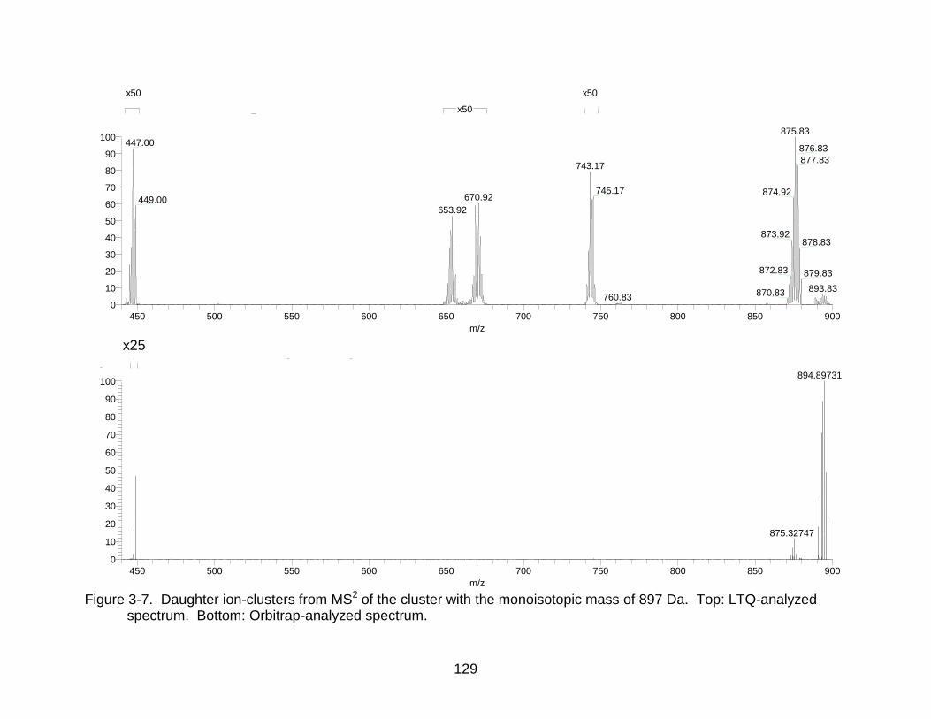
129
Figure 3-7. Daughter ion-clusters from MS2 of the cluster with the monoisotopic mass of 897 Da. Top: LTQ-analyzed spectrum. Bottom: Orbitrap-analyzed spectrum.
CID_895_width_8_Pb_L8_E2_090414175306 #1-150 RT: 0.00-4.94 AV: 150 NL: 6.14E5T: FTMS + p MALDI Full ms2 [email protected] [245.00-925.00]
450 500 550 600 650 700 750 800 850 900
m/z
0
10
20
30
40
50
60
70
80
90
100
Re
lative
Ab
un
da
nce
894.89731
875.32747
x25
x50
PbBasic_MS2_894_wide_J7 #1-100 RT: 0.00-1.68 AV: 100 NL: 4.49E3T: ITMS + p MALDI Full ms2 [email protected] [245.00-920.00]
450 500 550 600 650 700 750 800 850 900
m/z
0
10
20
30
40
50
60
70
80
90
100
Re
lative
Ab
un
da
nce
875.83
876.83
877.83
874.92
873.92878.83
872.83 879.83
893.83870.83
447.00
743.17
745.17670.92449.00
653.92
760.83
x50
x50
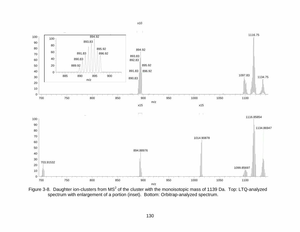
130
Figure 3-8. Daughter ion-clusters from MS2 of the cluster with the monoisotopic mass of 1139 Da. Top: LTQ-analyzed spectrum with enlargement of a portion (inset). Bottom: Orbitrap-analyzed spectrum.
PbBasic_MS2_1134_wide_J4 #1-100 RT: 0.00-1.71 AV: 100 NL: 3.49E3T: ITMS + p MALDI Full ms2 [email protected] [310.00-1155.00]
700 750 800 850 900 950 1000 1050 1100
m/z
0
10
20
30
40
50
60
70
80
90
100
Re
lative
Ab
un
da
nce
1116.75
1097.831134.75
894.92
893.83
892.83
895.92
891.83 896.92
890.83
PbBasic_MS2_1134_wide_J4 #1-100 RT: 0.00-1.71 AV:T: ITMS + p MALDI Full ms2 [email protected] [310.00- ...
885 890 895 900
m/z
0
20
40
60
80
100
Re
lative
Ab
un
da
nce
894.92
893.83
895.92
891.83 896.92
890.83
889.92
x10
x15 x15 Pb_pigment_CID_1135_CE75_Width16_L35 #1-200 RT: 0.07-13.19 AV: 200 NL: 8.62E4T: FTMS + p MALDI Full ms2 [email protected] [310.00-1150.00]
700 750 800 850 900 950 1000 1050 1100
m/z
0
10
20
30
40
50
60
70
80
90
100
Re
lative
Ab
un
da
nce
1116.85854
1134.86947
703.91532
1099.85697
1014.90878
894.88976
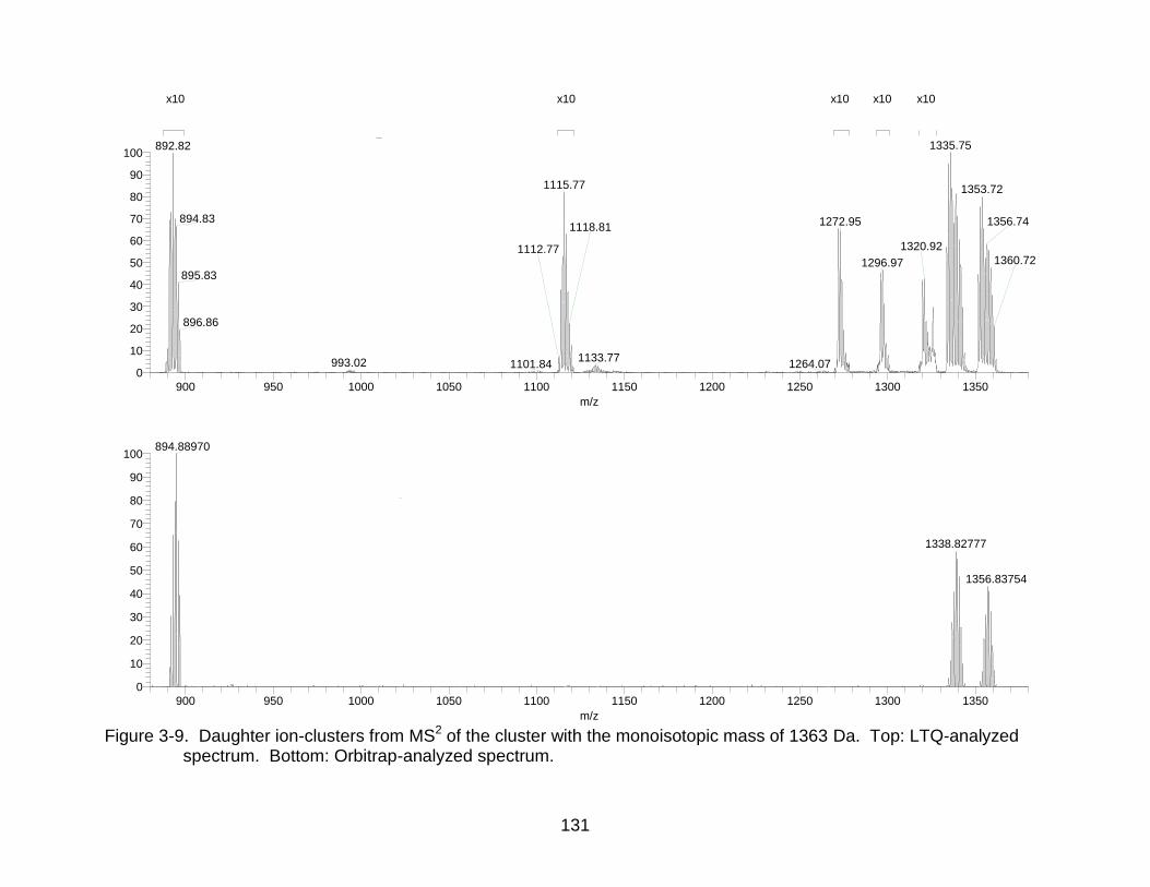
131
Figure 3-9. Daughter ion-clusters from MS2 of the cluster with the monoisotopic mass of 1363 Da. Top: LTQ-analyzed spectrum. Bottom: Orbitrap-analyzed spectrum.
WA_MS2_1358_CID_50_Width14_L35_E6 #1-37 RT: 0.00-2.53 AV: 37 NL: 2.11E5T: FTMS + p MALDI w Full ms2 [email protected] [370.00-1400.00]
900 950 1000 1050 1100 1150 1200 1250 1300 1350
m/z
0
10
20
30
40
50
60
70
80
90
100
Re
lative
Ab
un
da
nce
894.88970
1338.82777
1356.83754
x10 x10 x10 x10 PbBasic_MS2_1358_wide_J4_080718180033 #1-100 RT: 0.00-1.68 AV: 100 NL: 3.81E2T: ITMS + p MALDI Full ms2 [email protected] [370.00-1380.00]
900 950 1000 1050 1100 1150 1200 1250 1300 1350
m/z
0
10
20
30
40
50
60
70
80
90
100
Re
lative
Ab
un
da
nce
1335.75
1353.72
1356.74
1360.72
892.82
1115.77
1272.95894.83
1296.97
1320.92
1133.77
895.83
1118.81
896.86
993.02 1264.07
1112.77
1101.84
x10
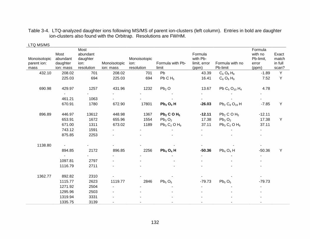
132
Table 3-4. LTQ-analyzed daughter ions following MS/MS of parent ion-clusters (left column). Entries in bold are daughter ion-clusters also found with the Orbitrap. Resolutions are FWHM.
LTQ MS/MS
Monoisotopic parent ion: mass
Most abundant daughter ion: mass
Most abundant daughter ion: resolution
Monoisotopic ion: mass
Monoisotopic ion: resolution
Formula with Pb-limit
Formula with Pb-limit, error (ppm)
Formula with no Pb-limit
Formula with no Pb-limit, error (ppm)
Exact match in full scan?
432.10 208.02 701 208.02 701 Pb 43.39 C6 O8 H8 -1.89 Y
225.03 694 225.03 694 Pb C H5 16.41 C6 O9 H9 7.52 Y
690.98 429.97 1257 431.96 1232 Pb2 O 13.67 Pb C5 O10 H4 4.78
- - - - - - - -
461.21 1063 - - - - - -
670.91 1780 672.90 17801 Pb3 O3 H -26.03 Pb2 C8 O19 H -7.85 Y
896.89 446.97 13612 448.98 1367 Pb2 C O H5 -12.11 Pb2 C O H5 -12.11
653.91 1672 655.96 1554 Pb3 O2 17.38 Pb3 O2 17.38 Y
671.00 1311 673.02 1189 Pb3 C2 O H9 37.11 Pb3 C2 O H9 37.11
743.12 1591 - - - - - -
875.85 2253 - - - - - -
1138.80 - - - - - - - -
894.85 2172 896.85 2256 Pb4 O4 H -50.36 Pb4 O4 H -50.36 Y
- - - - - - - -
1097.81 2797 - - - - - -
1116.79 2711 - - - - - -
1362.77 892.82 2310 - - - - - -
1115.77 2623 1119.77 2846 Pb5 O5 -79.73 Pb5 O5 -79.73
1271.92 2504 - - - - - -
1295.96 2503 - - - - - -
1319.94 3331 - - - - - -
1335.75 3139 - - - - - -
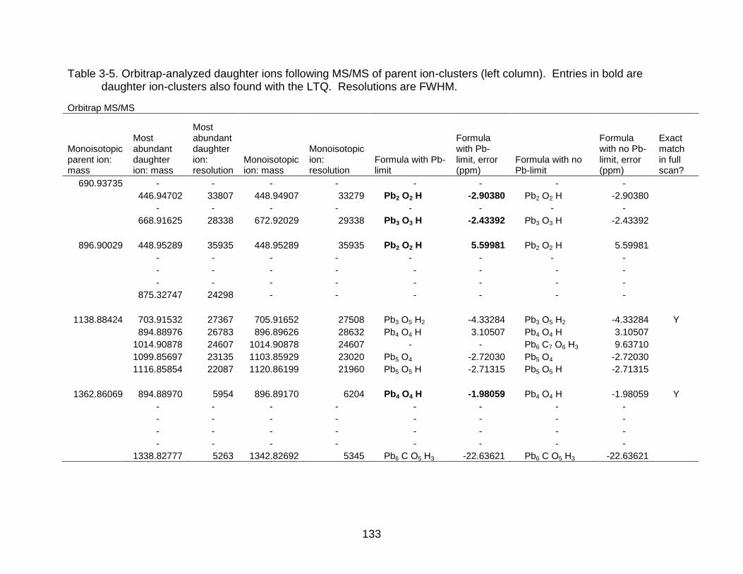
133
Table 3-5. Orbitrap-analyzed daughter ions following MS/MS of parent ion-clusters (left column). Entries in bold are daughter ion-clusters also found with the LTQ. Resolutions are FWHM.
Orbitrap MS/MS
Monoisotopic parent ion: mass
Most abundant daughter ion: mass
Most abundant daughter ion: resolution
Monoisotopic ion: mass
Monoisotopic ion: resolution
Formula with Pb-limit
Formula with Pb-limit, error (ppm)
Formula with no Pb-limit
Formula with no Pb-limit, error (ppm)
Exact match in full scan?
690.93735 - - - - - - - -
446.94702 33807 448.94907 33279 Pb2 O2 H -2.90380 Pb2 O2 H -2.90380
- - - - - - - -
668.91625 28338 672.92029 29338 Pb3 O3 H -2.43392 Pb3 O3 H -2.43392
896.90029 448.95289 35935 448.95289 35935 Pb2 O2 H 5.59981 Pb2 O2 H 5.59981
- - - - - - - -
- - - - - - - -
- - - - - - - -
875.32747 24298 - - - - - -
1138.88424 703.91532 27367 705.91652 27508 Pb3 O5 H2 -4.33284 Pb3 O5 H2 -4.33284 Y
894.88976 26783 896.89626 28632 Pb4 O4 H 3.10507 Pb4 O4 H 3.10507
1014.90878 24607 1014.90878 24607 - - Pb6 C7 O6 H3 9.63710
1099.85697 23135 1103.85929 23020 Pb5 O4 -2.72030 Pb5 O4 -2.72030
1116.85854 22087 1120.86199 21960 Pb5 O5 H -2.71315 Pb5 O5 H -2.71315
1362.86069 894.88970 5954 896.89170 6204 Pb4 O4 H -1.98059 Pb4 O4 H -1.98059 Y
- - - - - - - -
- - - - - - - -
- - - - - - - -
- - - - - - - -
1338.82777 5263 1342.82692 5345 Pb6 C O5 H3 -22.63621 Pb6 C O5 H3 -22.63621
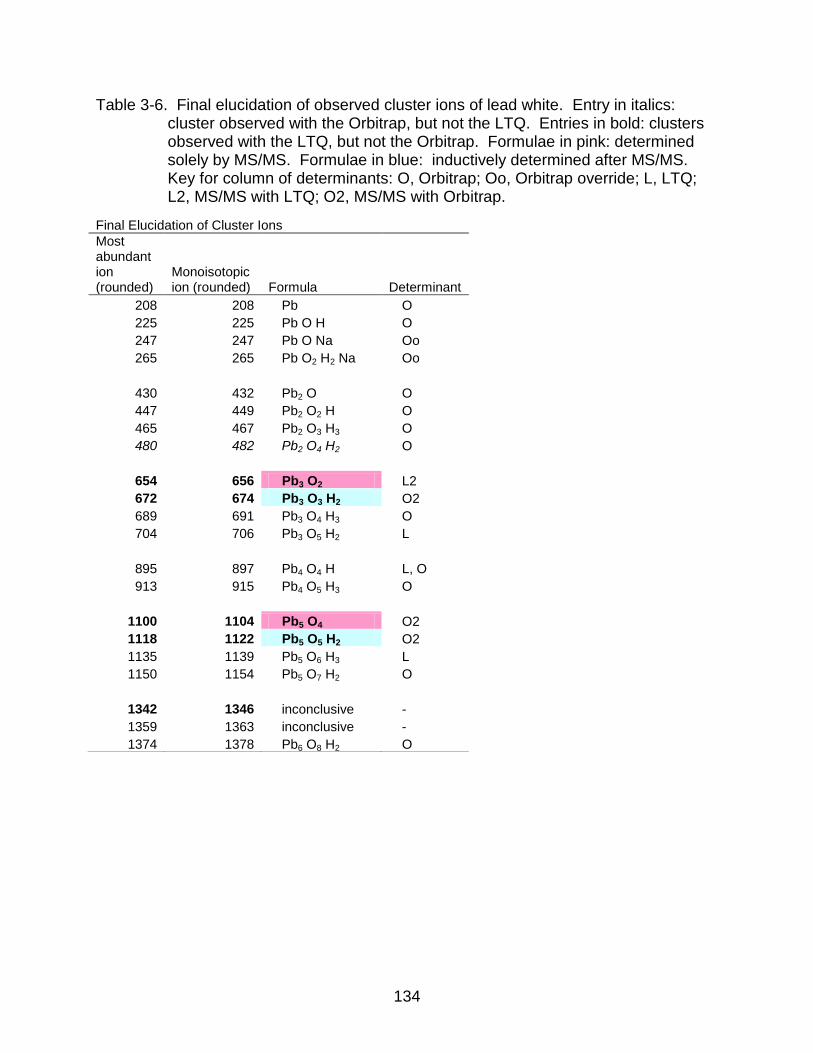
134
Table 3-6. Final elucidation of observed cluster ions of lead white. Entry in italics: cluster observed with the Orbitrap, but not the LTQ. Entries in bold: clusters observed with the LTQ, but not the Orbitrap. Formulae in pink: determined solely by MS/MS. Formulae in blue: inductively determined after MS/MS. Key for column of determinants: O, Orbitrap; Oo, Orbitrap override; L, LTQ; L2, MS/MS with LTQ; O2, MS/MS with Orbitrap.
Final Elucidation of Cluster Ions
Most abundant ion (rounded)
Monoisotopic ion (rounded) Formula Determinant
208 208 Pb O
225 225 Pb O H O
247 247 Pb O Na Oo
265 265 Pb O2 H2 Na Oo
430 432 Pb2 O O
447 449 Pb2 O2 H O
465 467 Pb2 O3 H3 O
480 482 Pb2 O4 H2 O
654 656 Pb3 O2 L2
672 674 Pb3 O3 H2 O2
689 691 Pb3 O4 H3 O
704 706 Pb3 O5 H2 L
895 897 Pb4 O4 H L, O
913 915 Pb4 O5 H3 O
1100 1104 Pb5 O4 O2
1118 1122 Pb5 O5 H2 O2
1135 1139 Pb5 O6 H3 L
1150 1154 Pb5 O7 H2 O
1342 1346 inconclusive -
1359 1363 inconclusive -
1374 1378 Pb6 O8 H2 O
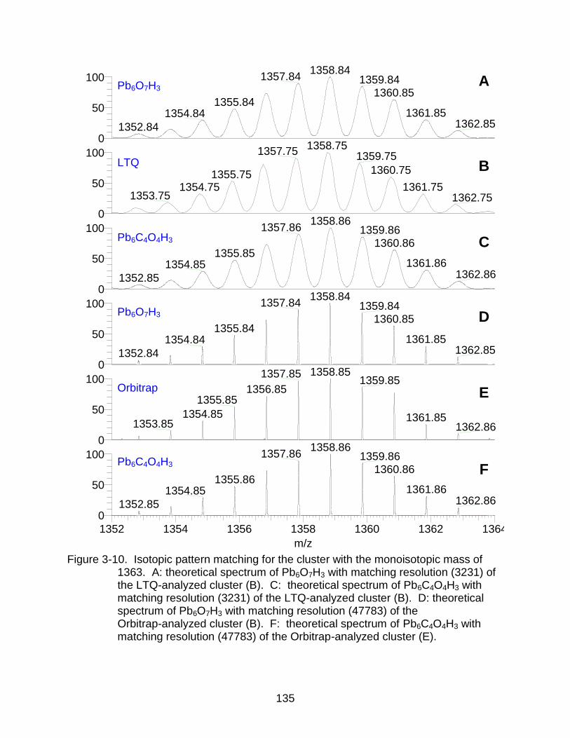
135
Figure 3-10. Isotopic pattern matching for the cluster with the monoisotopic mass of 1363. A: theoretical spectrum of Pb6O7H3 with matching resolution (3231) of the LTQ-analyzed cluster (B). C: theoretical spectrum of Pb6C4O4H3 with matching resolution (3231) of the LTQ-analyzed cluster (B). D: theoretical spectrum of Pb6O7H3 with matching resolution (47783) of the Orbitrap-analyzed cluster (B). F: theoretical spectrum of Pb6C4O4H3 with matching resolution (47783) of the Orbitrap-analyzed cluster (E).
1352 1354 1356 1358 1360 1362 1364
m/z
0
50
100
0
50
100
0
50
100
0
50
100
Re
lative
Ab
un
da
nce 0
50
100
0
50
1001358.84
1357.84 1359.841360.85
1355.841361.851354.84
1362.851352.84
1358.751357.75 1359.75
1360.751355.751361.751354.75
1353.75 1362.75
1358.861357.86 1359.86
1360.861355.85
1361.861354.851362.861352.85
1358.841357.84 1359.84
1360.851355.84
1361.851354.841362.851352.84
1358.851357.851359.85
1356.851355.85
1354.85 1361.851353.85 1362.86
1358.861357.86 1359.86
1360.861355.86
1361.861354.851362.861352.85
NL:4.22E3
Pb 6 O 7 H 3: Pb 6 O 7 H 3
p (gss, s /p:40) Chrg 1R: 3231 Res .Pwr . @FWHMNL:1.45E4
Pb10x_normal_J1#1-50 RT: 0.00-0.38 AV: 50 T: ITMS + p MALDI Full ms [100.00-2000.00]
NL:4.21E3
Pb 6 C 4 O 4 H 3: Pb 6 C 4 O 4 H 3
p (gss, s /p:40) Chrg 1R: 3231 Res .Pwr . @FWHMNL:4.21E3
Pb 6 O 7 H 3: Pb 6 O 7 H 3
p (gss, s /p:40) Chrg 1R: 47783 Res .Pwr . @FWHMNL:2.69E5
ms_undil_pb_l15_e2#10 RT: 0.38 AV: 1 T: FTMS + p MALDI Full ms [50.00-2000.00]
NL:4.20E3
Pb 6 C 4 O 4 H 3: Pb 6 C 4 O 4 H 3
p (gss, s /p:40) Chrg 1R: 47783 Res .Pwr . @FWHM
A
B
C
D
E
F
Pb6O7H3
LTQ
Pb6C4O4H3
Pb6O7H3
Orbitrap
Pb6C4O4H3
136
CHAPTER 4 LASER DESORPTION/IONIZATION-TANDEM MASS SPECTROMETRY OF MADDER
AND LEAD WHITE DIRECTLY FROM ARTISTIC SAMPLES
Background
The mass spectrometric analysis of artistic samples often garners interest from the
general public due to its appeal as a practical technology to preserve objects of cultural
heritage, rather than as an unapproachably esoteric chemistry experiment. Such
analyses also win acclaim from the scientific community as way to make known the
universal application of chemistry to preserve empathetic objects of beauty. Yet,
interest in the analysis of artistic samples must be limited and focused: its novelty lies
not necessarily with either the advancement or application of new technologies, but with
the new sets of information obtained from such analyses for the conservation science
community, which includes conservators, curators, and art historians. To the analytical
chemist, particularly the analytical mass spectrometrist, artistic samples are simply
another genre of analysis, whether it be derived from direct interrogation or following
extraction, separation, or derivatization. It is not significantly different from the analysis
of neat samples, geological specimens, or biological tissues.
Considering the above perspective on the mass spectrometric analysis of artistic
samples, any attempt at an exhaustive review of the literature, such as was conducted
for Chapters 2 and 3, would be unnecessarily cumbersome. Therefore, only a cursory
review shall be provided, focusing on desorption/ionization methods applied directly to
artistic samples of textile fibers and painting cross sections. For a primer on the
application of analytical chemistry for artistic samples and, more broadly, for the
preservation of art and archaeological objects, the reader is referred to an existing
selection of books2-4,53,117,162,163 on this topic.
137
Desorption/ionization methods such as laser desorption/ionization (LDI),
secondary ion mass spectrometry (SIMS), and direct analysis in real time (DART) have
been conducted on samples and surfaces such as fibers77, textiles71, newspaper74,
illuminated manuscripts74,76, ancient cosmetics123, ceramics9, statuettes164, and painting
cross sections74,77,165-170. Other direct MS methods used to characterize art objects
include laser ablation-inductively coupled plasma MS on glass119 and matrix-assisted
laser desorption/ionization (MALDI) on painting fragments171. Many of the other direct
analytical methods for artistic samples are spectroscopic, including Raman, infrared (IR)
and its Fourier transform variant (FTIR), X-ray fluorescence, and particle-induced X-ray
emission (PIXE).2-4
Crucial for the work presented in this Chapter is the precedence of direct
analyses of painting cross sections and textiles. Attention must be given to relevant
direct analyses with respect to their sample preparation and introduction, since both
seem to be the only real novelty gleaned from such experiments. Although seemingly
important, ionization and instrumental settings established in the literature are not
necessarily worthy of note for two reasons. First, the majority of direct analyses have
been conducted with SIMS for imaging experiments, which is not the method employed
here. Second, the LDI74,76,77 analyses followed the standard, long-espoused practice of
using minimal laser fluence, such that it is just above the ionization threshold and below
the fluence causing in-source fragmentation and noise. As Wyplosz mentioned in his
thorough dissertation77, an important aspect to consider for painting cross sections is
the surface morphology and localization of pigments or dyes, which may alter
138
spot-to-spot variation, and the risk of ablating away the sample, which is critically
important for precious samples.
To account for the peculiar morphology and topography of artistic samples,
particularly painting cross sections, and to allow these samples to be effectively
introduced into the vacuum chamber of an instrument’s ionization region, four methods
have generally been employed. The most rudimentary method is to simply affix the
unaltered sample to the sample plate using double-sided tape, which has been applied
to painting cross sections.74,77 Wyplosz created and used a specially modified sample
holder to support fiber samples.77 In Grim’s dissertation, she immersed a chip from a
painting in linseed oil atop the sample plate.74 A necessity for SIMS analysis is to
create a smooth, flat surface by slicing or polishing the sample.9 To aid in the creation
of a flat surface for SIMS, the popular method of first embedding the sample in a
polymer resin is often used164-170, and with some variation such as washing the sample
with hexane to remove contaminants9,165-168 and coating the sample with sputtered
gold165,168.
Considering that only LDI was used in the work presented here, the simple method
of affixing unaltered chips from paintings and fabrics with double-sided tape was used
with adequate results. The analyses were conducted to determine if the pigment lead
white and the dye alizarin were detectable in chips of both authentic and experimental
paintings, and if components of madder (i.e., alizarin or purpurin) were detectable in
dyed fabrics of silk. For a comprehensive review of the LDI-mass spectrometric
analysis of alizarin and lead white, the reader is referred to Chapter 2 and 3 in this
dissertation, respectively. Briefly, the in situ detection by LDI of alizarin was attempted
139
by Wyplosz in his 2003 dissertation.77 His analysis of alizarin in a painting produced no
significant ions, but his analysis of an ancient dyed fiber did show an abundant ion
indicative of alizarin; in both samples, tandem mass spectrometry (MS/MS) was not
attempted despite the use of an ion trap. The 2003 dissertation by Grim did show some
LDI-ToF-generated spectra from a paint chip that may have been indicative of lead
white, but she was unable to conclude that the signal did not originate from two
competing lead-containing pigments, lead chromate (PbCrO4) or red lead (Pb3O4).74
There has been no published work on the in situ detection by LDI of lead white thus far;
what follows is the first-time LDI-tandem mass spectrometric detection of
(laser-reduced) alizarin from samples of both a painting and dyed textile, and the first
ever LDI detection of lead white from a painting sample, all without any sample
preparation whatsoever.
Experimental Methods
Samples: Painting Fragments and Dyed Silk Swatches
Several samples of paintings, from both historical and experimental paintings,
and swatches of dyed silk were donated by Julie Arslanoglu, conservation scientist at
The Metropolitan Museum of Art, New York, NY, and are shown in Figure 4-1. The
provided descriptions for samples I–VII follows.
I: Paint composition: linseed oil and alizarin in a single layer. Ground: calcium sulfate and gelatine on panel. Created: 1997. II: Paint composition: linseed oil and alizarin, possibly more than one layer of paint. Ground: calcium sulfate and gelatine on panel. Created: 1997. III: Silk fabric dyes with madder, which contains alizarin and purpurin. IV: Silk fabric probably dyed with munjeet, which contains alizarin and purpurin.
140
V: Paint composition: unknown paint and oil in multiple layers with wax. Ground: calcium carbonate and collagen glue. Created: 15th century with extensive restoration. VI: Paint composition: lead white in oil with a dammar varnish. Ground: board. VII: Paint composition: yellow ochre (FeO(OH)), linseed oil, and elemi (resin). Ground: paper. Created: 2006. All samples were untreated and affixed with double-sided adhesive tape to either
a glass microscope slide or directly on the steel sample plate, which was machined to a
lower height to fit a microscope slide.
Laser Desorption/Ionization Parameters
All laser desorption/ionization experiments were performed on a Thermo
Finnigan LTQ-XL (San Jose, CA) equipped with an intermediate-pressure source and a
N2 laser ( = 337 nm). For all samples and for both full-scan and tandem mass
spectrometry, the laser was attenuated to the lowest power just above the ionization
threshold, which varied by sample, but was typically set between 5.0 and 35 μJ per
pulse. Thus, the desired ionization metric of laser fluence can only be estimated
between 6.4 102 J/m2 and 4.5 103 J/m2 due to the difficulty in an accurate and precise
measurement of the laser spot size, which has an approximate 100-μm spot. Automatic
gain control was set to limit the number of laser shots per analytical scan, which was
generated from just one microscan. After each analytical scan, the samples were
moved in a raster pattern with respect to the laser, within a user-defined area manually
selected via the software’s “imaging” mode.
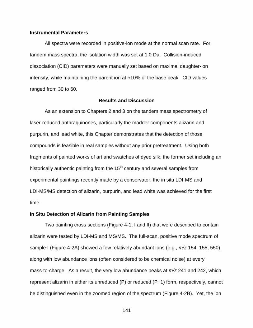
141
Instrumental Parameters
All spectra were recorded in positive-ion mode at the normal scan rate. For
tandem mass spectra, the isolation width was set at 1.0 Da. Collision-induced
dissociation (CID) parameters were manually set based on maximal daughter-ion
intensity, while maintaining the parent ion at ≈10% of the base peak. CID values
ranged from 30 to 60.
Results and Discussion
As an extension to Chapters 2 and 3 on the tandem mass spectrometry of
laser-reduced anthraquinones, particularly the madder components alizarin and
purpurin, and lead white, this Chapter demonstrates that the detection of those
compounds is feasible in real samples without any prior pretreatment. Using both
fragments of painted works of art and swatches of dyed silk, the former set including an
historically authentic painting from the 15th century and several samples from
experimental paintings recently made by a conservator, the in situ LDI-MS and
LDI-MS/MS detection of alizarin, purpurin, and lead white was achieved for the first
time.
In Situ Detection of Alizarin from Painting Samples
Two painting cross sections (Figure 4-1, I and II) that were described to contain
alizarin were tested by LDI-MS and MS/MS. The full-scan, positive mode spectrum of
sample I (Figure 4-2A) showed a few relatively abundant ions (e.g., m/z 154, 155, 550)
along with low abundance ions (often considered to be chemical noise) at every
mass-to-charge. As a result, the very low abundance peaks at m/z 241 and 242, which
represent alizarin in either its unreduced (P) or reduced (P+1) form, respectively, cannot
be distinguished even in the zoomed region of the spectrum (Figure 4-2B). Yet, the ion
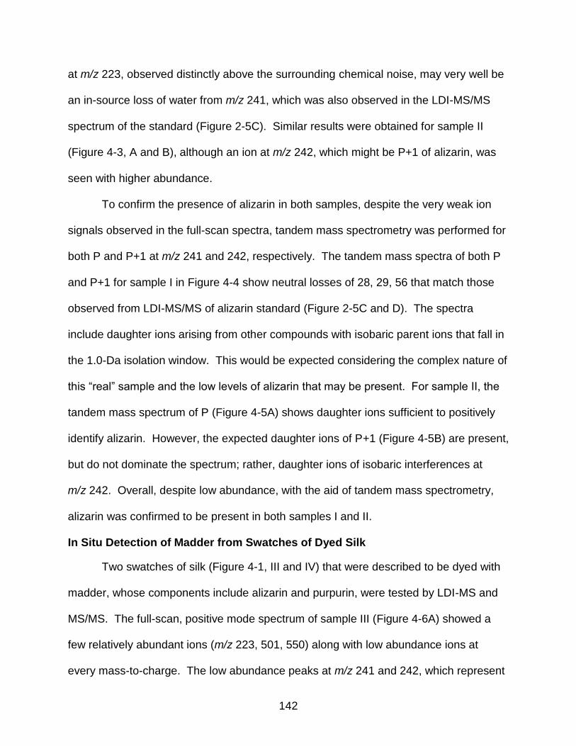
142
at m/z 223, observed distinctly above the surrounding chemical noise, may very well be
an in-source loss of water from m/z 241, which was also observed in the LDI-MS/MS
spectrum of the standard (Figure 2-5C). Similar results were obtained for sample II
(Figure 4-3, A and B), although an ion at m/z 242, which might be P+1 of alizarin, was
seen with higher abundance.
To confirm the presence of alizarin in both samples, despite the very weak ion
signals observed in the full-scan spectra, tandem mass spectrometry was performed for
both P and P+1 at m/z 241 and 242, respectively. The tandem mass spectra of both P
and P+1 for sample I in Figure 4-4 show neutral losses of 28, 29, 56 that match those
observed from LDI-MS/MS of alizarin standard (Figure 2-5C and D). The spectra
include daughter ions arising from other compounds with isobaric parent ions that fall in
the 1.0-Da isolation window. This would be expected considering the complex nature of
this “real” sample and the low levels of alizarin that may be present. For sample II, the
tandem mass spectrum of P (Figure 4-5A) shows daughter ions sufficient to positively
identify alizarin. However, the expected daughter ions of P+1 (Figure 4-5B) are present,
but do not dominate the spectrum; rather, daughter ions of isobaric interferences at
m/z 242. Overall, despite low abundance, with the aid of tandem mass spectrometry,
alizarin was confirmed to be present in both samples I and II.
In Situ Detection of Madder from Swatches of Dyed Silk
Two swatches of silk (Figure 4-1, III and IV) that were described to be dyed with
madder, whose components include alizarin and purpurin, were tested by LDI-MS and
MS/MS. The full-scan, positive mode spectrum of sample III (Figure 4-6A) showed a
few relatively abundant ions (m/z 223, 501, 550) along with low abundance ions at
every mass-to-charge. The low abundance peaks at m/z 241 and 242, which represent
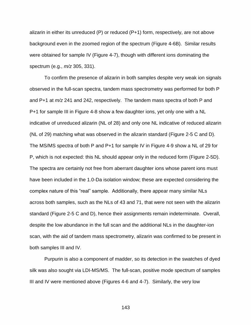
143
alizarin in either its unreduced (P) or reduced (P+1) form, respectively, are not above
background even in the zoomed region of the spectrum (Figure 4-6B). Similar results
were obtained for sample IV (Figure 4-7), though with different ions dominating the
spectrum (e.g., m/z 305, 331).
To confirm the presence of alizarin in both samples despite very weak ion signals
observed in the full-scan spectra, tandem mass spectrometry was performed for both P
and P+1 at m/z 241 and 242, respectively. The tandem mass spectra of both P and
P+1 for sample III in Figure 4-8 show a few daughter ions, yet only one with a NL
indicative of unreduced alizarin (NL of 28) and only one NL indicative of reduced alizarin
(NL of 29) matching what was observed in the alizarin standard (Figure 2-5 C and D).
The MS/MS spectra of both P and P+1 for sample IV in Figure 4-9 show a NL of 29 for
P, which is not expected: this NL should appear only in the reduced form (Figure 2-5D).
The spectra are certainly not free from aberrant daughter ions whose parent ions must
have been included in the 1.0-Da isolation window; these are expected considering the
complex nature of this “real” sample. Additionally, there appear many similar NLs
across both samples, such as the NLs of 43 and 71, that were not seen with the alizarin
standard (Figure 2-5 C and D), hence their assignments remain indeterminate. Overall,
despite the low abundance in the full scan and the additional NLs in the daughter-ion
scan, with the aid of tandem mass spectrometry, alizarin was confirmed to be present in
both samples III and IV.
Purpurin is also a component of madder, so its detection in the swatches of dyed
silk was also sought via LDI-MS/MS. The full-scan, positive mode spectrum of samples
III and IV were mentioned above (Figures 4-6 and 4-7). Similarly, the very low
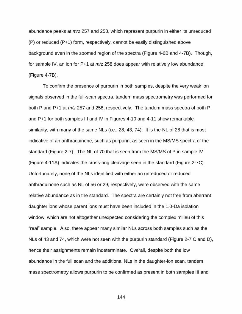
144
abundance peaks at m/z 257 and 258, which represent purpurin in either its unreduced
(P) or reduced (P+1) form, respectively, cannot be easily distinguished above
background even in the zoomed region of the spectra (Figure 4-6B and 4-7B). Though,
for sample IV, an ion for P+1 at m/z 258 does appear with relatively low abundance
(Figure 4-7B).
To confirm the presence of purpurin in both samples, despite the very weak ion
signals observed in the full-scan spectra, tandem mass spectrometry was performed for
both P and P+1 at m/z 257 and 258, respectively. The tandem mass spectra of both P
and P+1 for both samples III and IV in Figures 4-10 and 4-11 show remarkable
similarity, with many of the same NLs (i.e., 28, 43, 74). It is the NL of 28 that is most
indicative of an anthraquinone, such as purpurin, as seen in the MS/MS spectra of the
standard (Figure 2-7). The NL of 70 that is seen from the MS/MS of P in sample IV
(Figure 4-11A) indicates the cross-ring cleavage seen in the standard (Figure 2-7C).
Unfortunately, none of the NLs identified with either an unreduced or reduced
anthraquinone such as NL of 56 or 29, respectively, were observed with the same
relative abundance as in the standard. The spectra are certainly not free from aberrant
daughter ions whose parent ions must have been included in the 1.0-Da isolation
window, which are not altogether unexpected considering the complex milieu of this
“real” sample. Also, there appear many similar NLs across both samples such as the
NLs of 43 and 74, which were not seen with the purpurin standard (Figure 2-7 C and D),
hence their assignments remain indeterminate. Overall, despite both the low
abundance in the full scan and the additional NLs in the daughter-ion scan, tandem
mass spectrometry allows purpurin to be confirmed as present in both samples III and
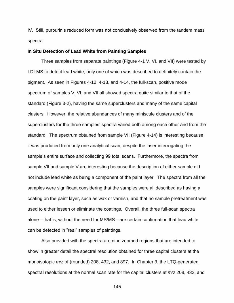
145
IV. Still, purpurin’s reduced form was not conclusively observed from the tandem mass
spectra.
In Situ Detection of Lead White from Painting Samples
Three samples from separate paintings (Figure 4-1 V, VI, and VII) were tested by
LDI-MS to detect lead white, only one of which was described to definitely contain the
pigment. As seen in Figures 4-12, 4-13, and 4-14, the full-scan, positive mode
spectrum of samples V, VI, and VII all showed spectra quite similar to that of the
standard (Figure 3-2), having the same superclusters and many of the same capital
clusters. However, the relative abundances of many miniscule clusters and of the
superclusters for the three samples’ spectra varied both among each other and from the
standard. The spectrum obtained from sample VII (Figure 4-14) is interesting because
it was produced from only one analytical scan, despite the laser interrogating the
sample’s entire surface and collecting 99 total scans. Furthermore, the spectra from
sample VII and sample V are interesting because the description of either sample did
not include lead white as being a component of the paint layer. The spectra from all the
samples were significant considering that the samples were all described as having a
coating on the paint layer, such as wax or varnish, and that no sample pretreatment was
used to either lessen or eliminate the coatings. Overall, the three full-scan spectra
alone—that is, without the need for MS/MS—are certain confirmation that lead white
can be detected in ”real” samples of paintings.
Also provided with the spectra are nine zoomed regions that are intended to
show in greater detail the spectral resolution obtained for three capital clusters at the
monoisotopic m/z of (rounded) 208, 432, and 897. In Chapter 3, the LTQ-generated
spectral resolutions at the normal scan rate for the capital clusters at m/z 208, 432, and
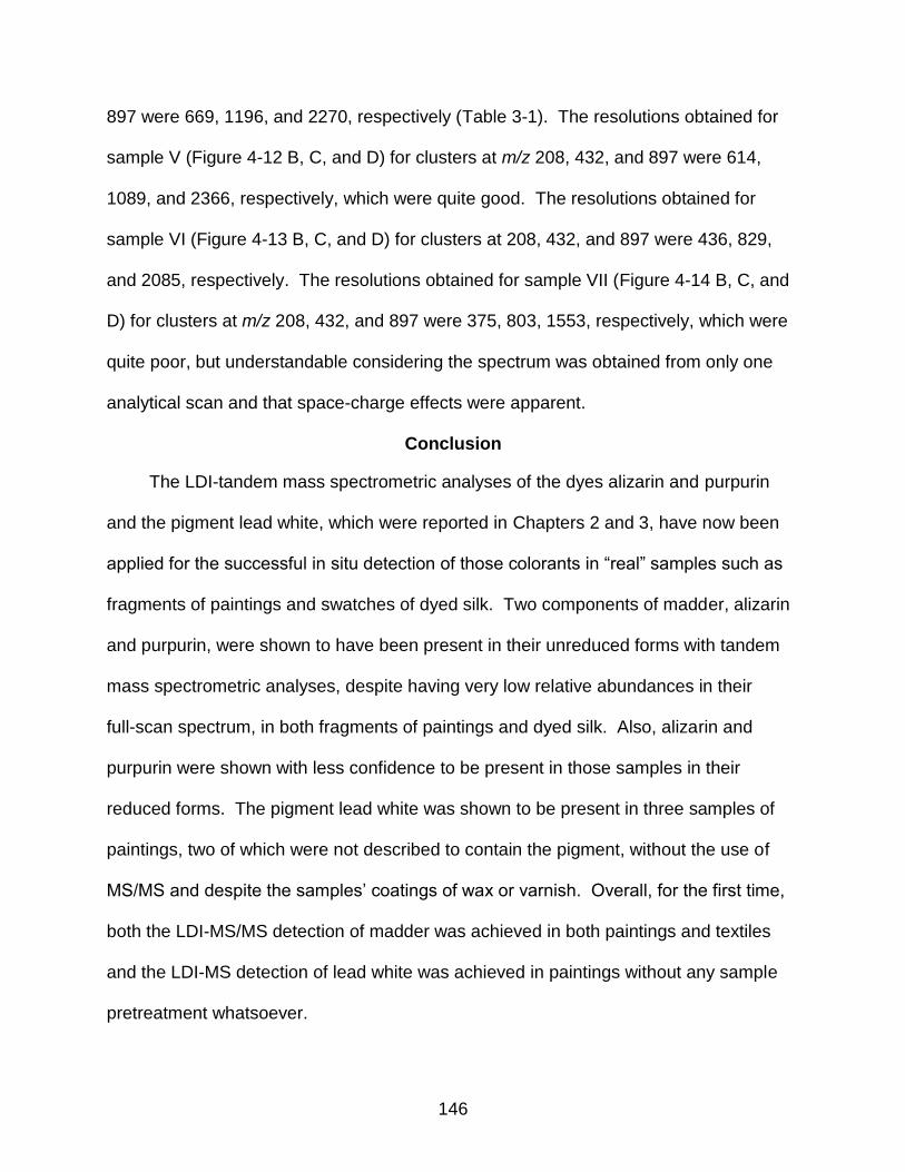
146
897 were 669, 1196, and 2270, respectively (Table 3-1). The resolutions obtained for
sample V (Figure 4-12 B, C, and D) for clusters at m/z 208, 432, and 897 were 614,
1089, and 2366, respectively, which were quite good. The resolutions obtained for
sample VI (Figure 4-13 B, C, and D) for clusters at 208, 432, and 897 were 436, 829,
and 2085, respectively. The resolutions obtained for sample VII (Figure 4-14 B, C, and
D) for clusters at m/z 208, 432, and 897 were 375, 803, 1553, respectively, which were
quite poor, but understandable considering the spectrum was obtained from only one
analytical scan and that space-charge effects were apparent.
Conclusion
The LDI-tandem mass spectrometric analyses of the dyes alizarin and purpurin
and the pigment lead white, which were reported in Chapters 2 and 3, have now been
applied for the successful in situ detection of those colorants in “real” samples such as
fragments of paintings and swatches of dyed silk. Two components of madder, alizarin
and purpurin, were shown to have been present in their unreduced forms with tandem
mass spectrometric analyses, despite having very low relative abundances in their
full-scan spectrum, in both fragments of paintings and dyed silk. Also, alizarin and
purpurin were shown with less confidence to be present in those samples in their
reduced forms. The pigment lead white was shown to be present in three samples of
paintings, two of which were not described to contain the pigment, without the use of
MS/MS and despite the samples’ coatings of wax or varnish. Overall, for the first time,
both the LDI-MS/MS detection of madder was achieved in both paintings and textiles
and the LDI-MS detection of lead white was achieved in paintings without any sample
pretreatment whatsoever.
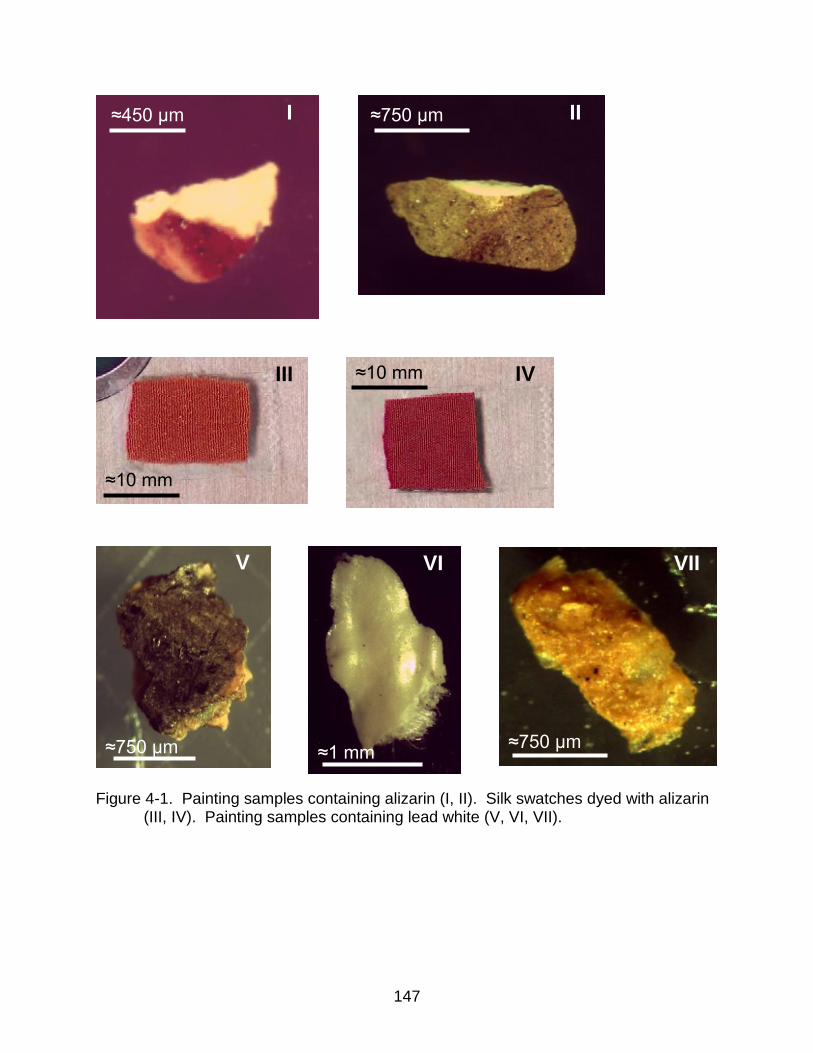
147
Figure 4-1. Painting samples containing alizarin (I, II). Silk swatches dyed with alizarin (III, IV). Painting samples containing lead white (V, VI, VII).
≈10 mm
III
≈750 μm II ≈450 μm I
≈10 mm IV
≈750 μm
V
≈750 μm
VII
≈1 mm
VI
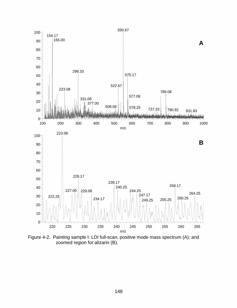
148
Figure 4-2. Painting sample I: LDI full-scan, positive mode mass spectrum (A); and zoomed region for alizarin (B).
A_surface_TI #1-25 RT: 0.00-0.35 AV: 25 NL: 9.82E1T: ITMS + p MALDI Full ms [50.00-2000.00]
220 225 230 235 240 245 250 255 260 265
m/z
0
10
20
30
40
50
60
70
80
90
100
Rela
tive A
bundance
223.08
228.17
239.17258.17240.25
227.00 244.25229.08264.25247.17222.25 260.25234.17 255.25249.25
A_surface_TI #1-25 RT: 0.00-0.35 AV: 25 NL: 3.12E2T: ITMS + p MALDI Full ms [50.00-2000.00]
100 200 300 400 500 600 700 800 900 1000
m/z
0
10
20
30
40
50
60
70
80
90
100
Re
lative
Abu
nd
an
ce
550.67
154.17155.00
298.33575.17
522.67223.08
789.08
577.08331.08
377.00508.58 578.25 737.33 790.92 931.83
A
B
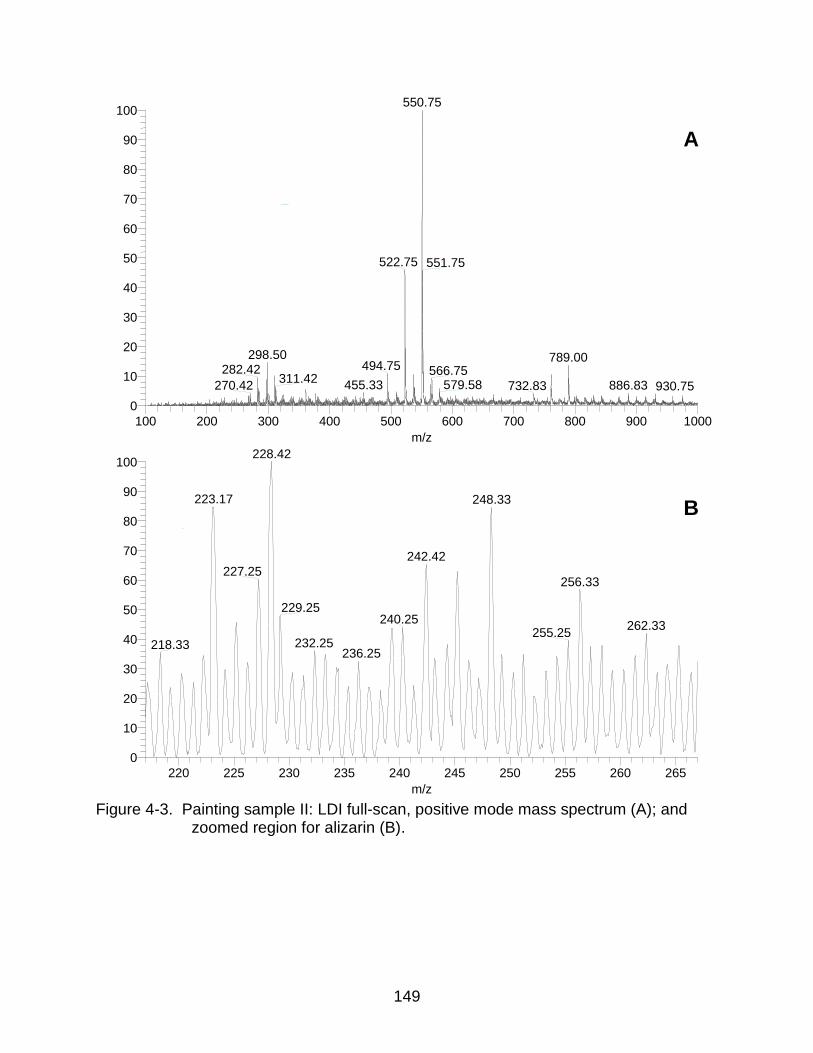
149
Figure 4-3. Painting sample II: LDI full-scan, positive mode mass spectrum (A); and zoomed region for alizarin (B).
B_surface_TI #1-25 RT: 0.00-0.31 AV: 25 NL: 2.09E2T: ITMS + p MALDI Full ms [50.00-1000.00]
220 225 230 235 240 245 250 255 260 265
m/z
0
10
20
30
40
50
60
70
80
90
100
Rela
tive A
bundance
228.42
223.17 248.33
242.42
227.25256.33
229.25240.25
262.33255.25
232.25218.33236.25
B_surface_TI #1-25 RT: 0.00-0.31 AV: 25 NL: 7.29E3T: ITMS + p MALDI Full ms [50.00-1000.00]
100 200 300 400 500 600 700 800 900 1000
m/z
0
10
20
30
40
50
60
70
80
90
100
Re
lative
Abu
nd
an
ce
550.75
522.75 551.75
298.50 789.00494.75282.42 566.75
311.42579.58455.33 886.83270.42 732.83 930.75
A
B
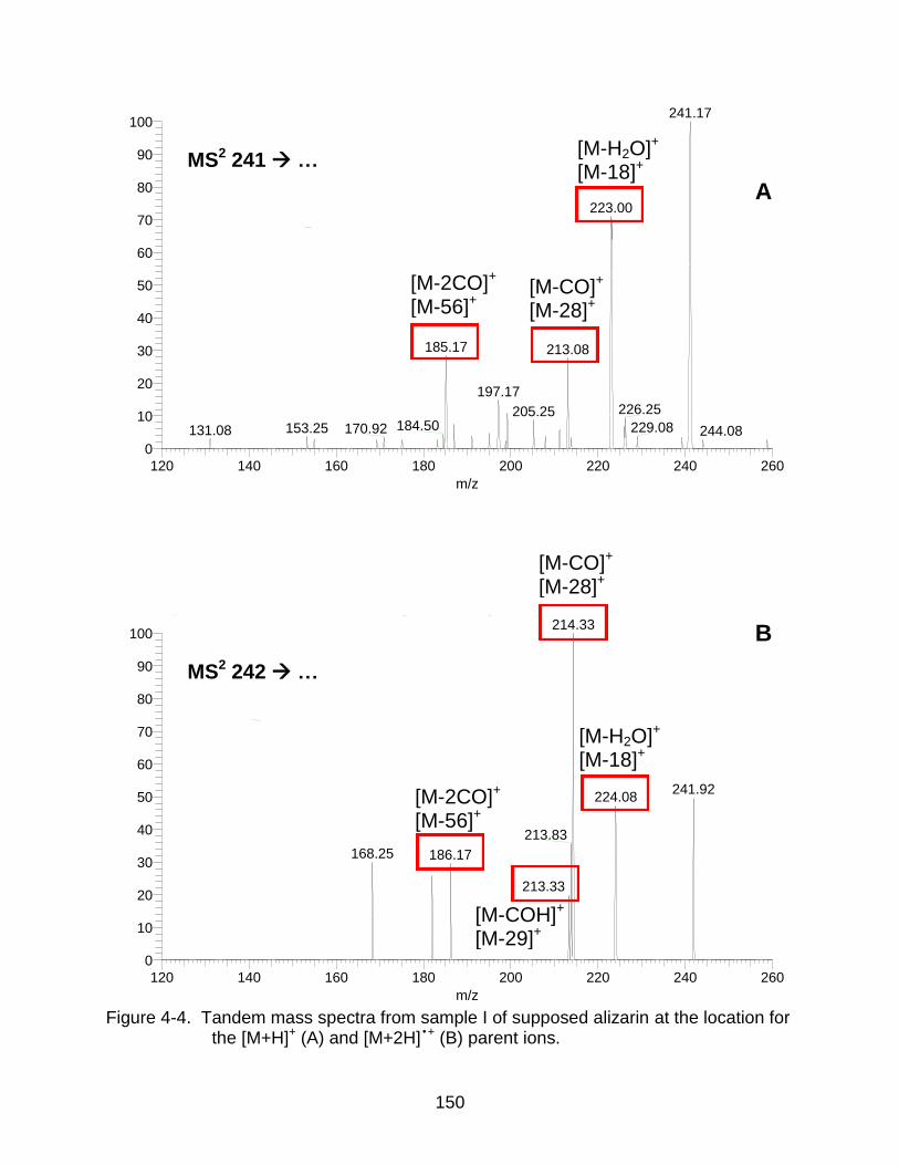
150
Figure 4-4. Tandem mass spectra from sample I of supposed alizarin at the location for the [M+H]+ (A) and [M+2H] •+ (B) parent ions.
A_MS2_242_TI_090127152321 #1-66 RT: 0.00-0.76 AV: 66 NL: 7.45E-1T: ITMS + p MALDI Full ms2 [email protected] [65.00-260.00]
120 140 160 180 200 220 240 260
m/z
0
10
20
30
40
50
60
70
80
90
100
Re
lative
Abu
nd
an
ce
214.33
241.92224.08
213.83
168.25 186.17
213.33
A_MS2_241_TI #1-39 RT: 0.00-0.47 AV: 39 NL: 1.09E1T: ITMS + p MALDI Full ms2 [email protected] [65.00-260.00]
120 140 160 180 200 220 240 260
m/z
0
10
20
30
40
50
60
70
80
90
100
Rela
tive A
bund
ance
241.17
223.00
185.17 213.08
197.17
226.25205.25184.50 229.08153.25 170.92131.08 244.08
[M-H2O]+ [M-18]+
[M-CO]+ [M-28]+
A
B
MS2 241 …
MS2 242 …
[M-CO]+ [M-28]+
[M-2CO]+ [M-56]+
[M-H2O]+ [M-18]+
[M-2CO]+ [M-56]+
[M-COH]+ [M-29]+
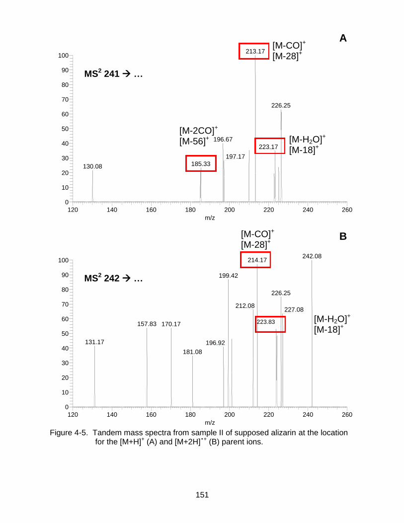
151
Figure 4-5. Tandem mass spectra from sample II of supposed alizarin at the location for the [M+H]+ (A) and [M+2H] •+ (B) parent ions.
B_MS2_241_TI #1-152 RT: 0.00-1.80 AV: 152 NL: 2.92E-1T: ITMS + p MALDI Full ms2 [email protected] [65.00-260.00]
120 140 160 180 200 220 240 260
m/z
0
10
20
30
40
50
60
70
80
90
100
Rela
tive A
bundance
213.17
226.25
196.67
223.17
197.17185.33130.08
A
B B_MS2_242_TI #1-151 RT: 0.00-1.78 AV: 151 NL: 1.69E-1T: ITMS + p MALDI Full ms2 [email protected] [65.00-260.00]
120 140 160 180 200 220 240 260
m/z
0
10
20
30
40
50
60
70
80
90
100
Re
lative
Abu
nd
an
ce
242.08214.17
199.42
226.25
212.08227.08
157.83 170.17
131.17 196.92
181.08
[M-2CO]+ [M-56]+ [M-H2O]+
[M-18]+
[M-CO]+ [M-28]+
MS2 241 …
MS2 242 …
[M-CO]+ [M-28]+
223.83 [M-H2O]+ [M-18]+
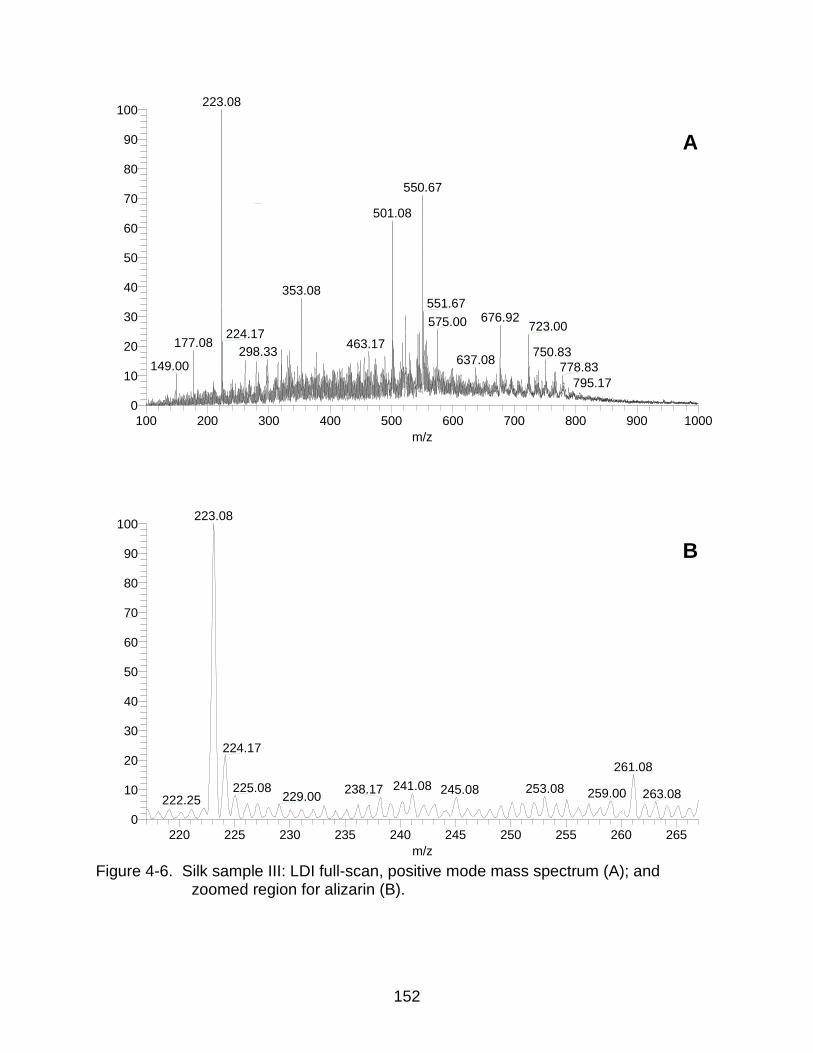
152
Figure 4-6. Silk sample III: LDI full-scan, positive mode mass spectrum (A); and zoomed region for alizarin (B).
A
Sample3_fullscan_LE11_TI #1-100 RT: 0.00-0.83 AV: 100 NL: 9.88E3T: ITMS + p MALDI Full ms [50.00-1000.00]
100 200 300 400 500 600 700 800 900 1000
m/z
0
10
20
30
40
50
60
70
80
90
100
Re
lative
Abu
nd
an
ce
223.08
550.67
501.08
353.08551.67
676.92575.00 723.00224.17
177.08 463.17298.33 750.83
637.08149.00 778.83
795.17
Sample3_fullscan_LE11_TI #1-100 RT: 0.00-0.83 AV: 100 NL: 9.88E3T: ITMS + p MALDI Full ms [50.00-1000.00]
220 225 230 235 240 245 250 255 260 265
m/z
0
10
20
30
40
50
60
70
80
90
100
Re
lative
Abu
nd
an
ce
223.08
224.17
261.08
241.08225.08 253.08238.17 245.08 259.00 263.08229.00222.25
B
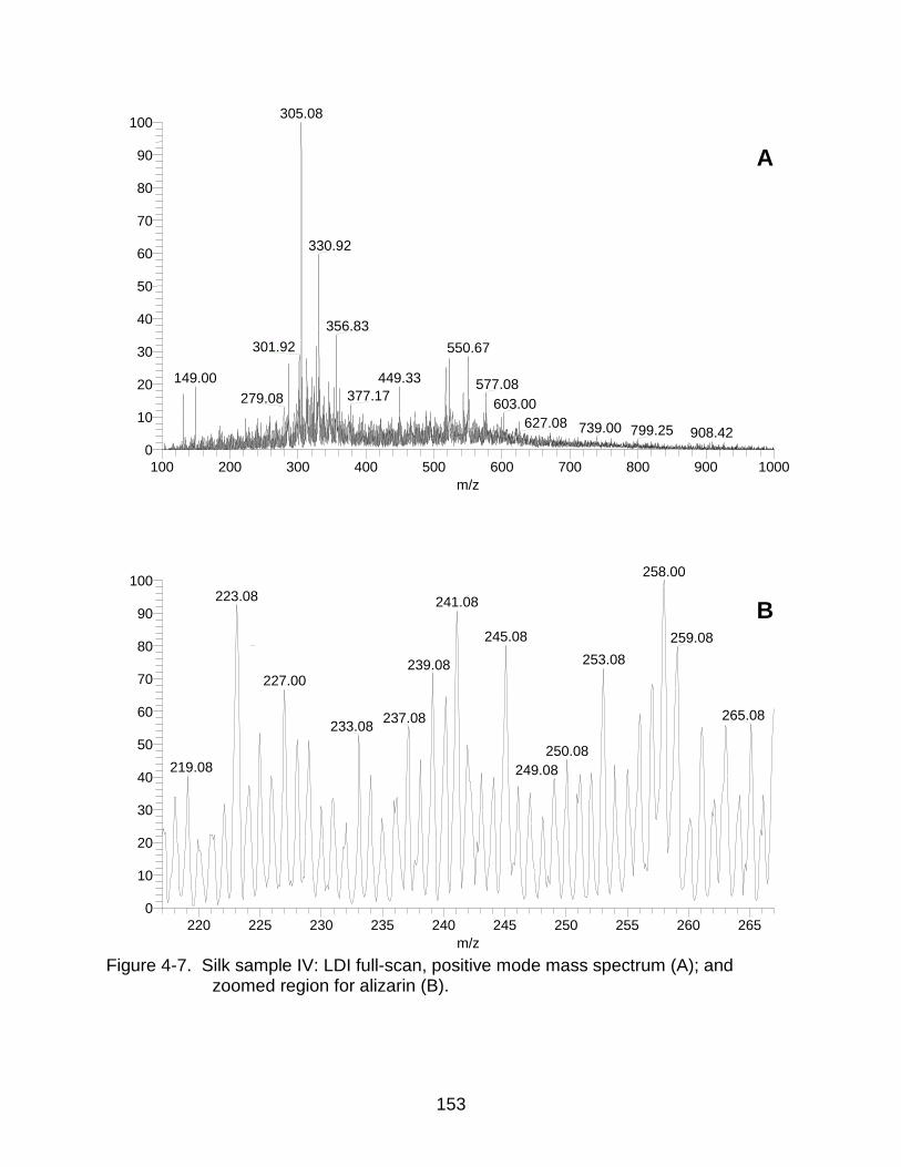
153
Figure 4-7. Silk sample IV: LDI full-scan, positive mode mass spectrum (A); and zoomed region for alizarin (B).
Sample5_full_scan_LE5_TI #1-101 RT: 0.00-1.14 AV: 101 NL: 2.92E3T: ITMS + p MALDI Full ms [50.00-1000.00]
100 200 300 400 500 600 700 800 900 1000
m/z
0
10
20
30
40
50
60
70
80
90
100
Re
lative
Abu
nd
an
ce
305.08
330.92
356.83
301.92 550.67
449.33149.00 577.08377.17279.08 603.00
627.08 739.00 799.25 908.42
Sample5_full_scan_LE5_TI #1-101 RT: 0.00-1.14 AV: 101 NL: 3.03E2T: ITMS + p MALDI Full ms [50.00-1000.00]
220 225 230 235 240 245 250 255 260 265
m/z
0
10
20
30
40
50
60
70
80
90
100
Re
lative
Abu
nd
an
ce
258.00
223.08 241.08
245.08 259.08
253.08239.08227.00
265.08237.08233.08
250.08219.08 249.08
A
B
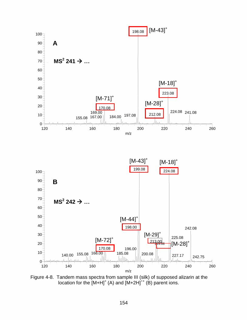
154
Figure 4-8. Tandem mass spectra from sample III (silk) of supposed alizarin at the location for the [M+H]+ (A) and [M+2H] •+ (B) parent ions.
Sample3_MS2_241_CID50_TI #1-101 RT: 0.00-1.22 AV: 101 NL: 2.60E2T: ITMS + p MALDI Full ms2 [email protected] [65.00-265.00]
120 140 160 180 200 220 240 260
m/z
0
10
20
30
40
50
60
70
80
90
100
Re
lative
Abu
nd
an
ce
198.08
223.08
170.08224.08169.00 241.08
212.08197.08184.00167.00155.08
Sample3_ms2_242_AGC_off_TI_121216160224 #1-101 RT: 0.00-0.61 AV: 101 NL: 2.45E2T: ITMS + p MALDI Full ms2 [email protected] [65.00-300.00]
120 140 160 180 200 220 240 260
m/z
0
10
20
30
40
50
60
70
80
90
100
Re
lative
Abu
nd
an
ce
199.08224.08
198.00 242.08
225.08213.00
170.08 196.00168.00 185.08 200.08155.08140.00 227.17 242.75
A
B
MS2 241 …
MS2 242 …
[M-18]+
[M-28]+
[M-43]+
[M-18]+ [M-43]+
[M-29]+
[M-71]+
[M-72]+
[M-44]+
[M-28]+ 214.08
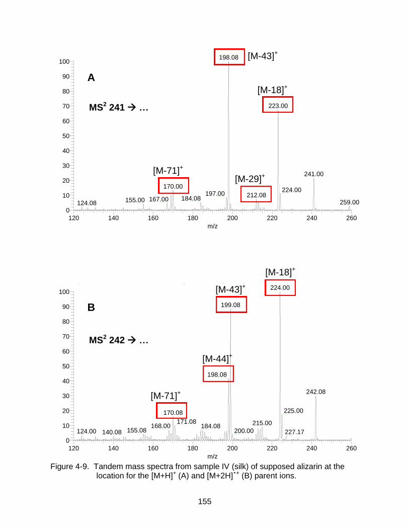
155
Figure 4-9. Tandem mass spectra from sample IV (silk) of supposed alizarin at the location for the [M+H]+ (A) and [M+2H] •+ (B) parent ions.
Sample5_ms2_241_AGC_off_TI _ 1 #1-101 RT: 0.00-0.62 AV: 101 NL: 4.37E3T: ITMS + p MALDI Full ms2 [email protected] [65.00-300.00]
120 140 160 180 200 220 240 260
m/z
0
10
20
30
40
50
60
70
80
90
100
Re
lative
Abu
nd
an
ce
198.08
223.00
241.00
170.00224.00
197.00 212.08184.08167.00155.00 259.00124.08
Sample5_ms2_242_AGC_off_TI #1-101 RT: 0.00-0.61 AV: 101 NL: 3.72E2T: ITMS + p MALDI Full ms2 [email protected] [65.00-300.00]
120 140 160 180 200 220 240 260
m/z
0
10
20
30
40
50
60
70
80
90
100
Re
lative
Abu
nd
an
ce
224.00
199.08
198.08
242.08
225.00170.08
171.08 215.00168.00 184.08155.08 200.00124.00 227.17140.08
A
B
MS2 241 …
MS2 242 …
[M-18]+
[M-18]+
[M-29]+ [M-71]+
[M-43]+
[M-44]+
[M-71]+
[M-43]+
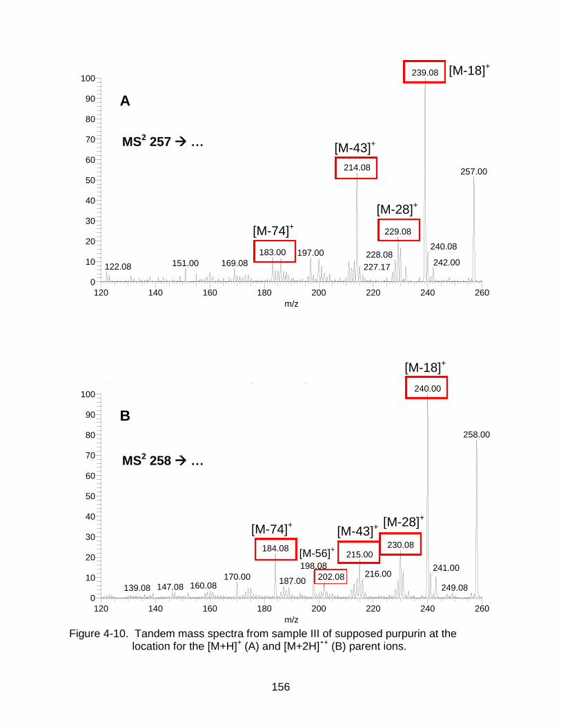
156
Figure 4-10. Tandem mass spectra from sample III of supposed purpurin at the location for the [M+H]+ (A) and [M+2H] •+ (B) parent ions.
Sample3_MS2_257_CID60_TI #1-100 RT: 0.00-1.22 AV: 100 NL: 5.28E1T: ITMS + p MALDI Full ms2 [email protected] [70.00-280.00]
120 140 160 180 200 220 240 260
m/z
0
10
20
30
40
50
60
70
80
90
100
Re
lative
Abu
nd
an
ce
239.08
214.08 257.00
229.08
240.08183.00 197.00 228.08
242.00169.08151.00122.08 227.17
Sample3_ms2_258_AGC_off_TI #1-100 RT: 0.00-0.61 AV: 100 NL: 5.42E2T: ITMS + p MALDI Full ms2 [email protected] [70.00-300.00]
120 140 160 180 200 220 240 260
m/z
0
10
20
30
40
50
60
70
80
90
100
Re
lative
Abu
nd
an
ce
240.00
258.00
230.08184.08215.00
198.08 241.00216.00170.00 202.08
187.00160.08147.08 249.08139.08
A
B
MS2 257 …
MS2 258 …
[M-28]+
[M-43]+
[M-18]+
[M-74]+
[M-74]+
[M-18]+
[M-43]+ [M-28]+
[M-56]+
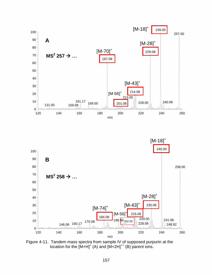
157
Figure 4-11. Tandem mass spectra from sample IV of supposed purpurin at the location for the [M+H]+ (A) and [M+2H] •+ (B) parent ions.
Sample5_ms2_258_AGC_off_TI #1-101 RT: 0.00-0.62 AV: 101 NL: 6.56E2T: ITMS + p MALDI Full ms2 [email protected] [70.00-300.00]
120 140 160 180 200 220 240 260
m/z
0
10
20
30
40
50
60
70
80
90
100
Re
lative
Abu
nd
an
ce
240.00
258.00
230.08
215.08184.08
229.00 241.08198.08170.08228.08160.17 248.92146.08
Sample5_ms2_257_AGC_off_TI #1-101 RT: 0.00-0.62 AV: 101 NL: 8.62E2T: ITMS + p MALDI Full ms2 [email protected] [70.00-300.00]
120 140 160 180 200 220 240 260
m/z
0
10
20
30
40
50
60
70
80
90
100
Re
lative
Abu
nd
an
ce
239.00
257.00
229.08
187.08
214.08
213.00
161.17 240.08228.00169.00 201.08131.00 159.08
A
B
MS2 257 …
MS2 258 …
[M-43]+
[M-28]+
[M-70]+
[M-74]+
[M-18]+
[M-28]+
[M-43]+
[M-18]+
[M-56]+
[M-56]+
202.00
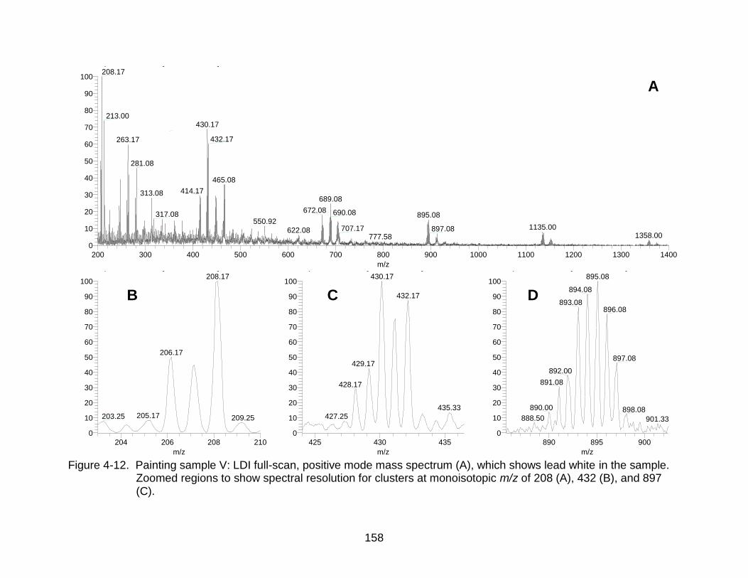
158
Figure 4-12. Painting sample V: LDI full-scan, positive mode mass spectrum (A), which shows lead white in the sample. Zoomed regions to show spectral resolution for clusters at monoisotopic m/z of 208 (A), 432 (B), and 897 (C).
D_surface_lp25_TI #1-70 RT: 0.00-1.25 AV: 70 NL: 7.49E2T: ITMS + p MALDI Full ms [100.00-2000.00]
200 300 400 500 600 700 800 900 1000 1100 1200 1300 1400
m/z
0
10
20
30
40
50
60
70
80
90
100
Rela
tive A
bundance
208.17
213.00430.17
432.17263.17
281.08
465.08
414.17313.08689.08
672.08 690.08317.08 895.08550.92
1135.00707.17 897.08622.081358.00777.58
D_surface_lp25_TI #1-70 RT: 0.00-1.25 AV: 70 NL:T: ITMS + p MALDI Full ms [100.00-2000.00]
204 206 208 210
m/z
0
10
20
30
40
50
60
70
80
90
100
Re
lative
Ab
un
da
nce
208.17
206.17
205.17203.25 209.25
D_surface_lp25_TI #1-70 RT: 0.00-1.25 AV: 70 NL:T: ITMS + p MALDI Full ms [100.00-2000.00]
425 430 435
m/z
0
10
20
30
40
50
60
70
80
90
100
Re
lative
Ab
un
da
nce
430.17
432.17
429.17
428.17
435.33427.25
D_surface_lp25_TI #1-70 RT: 0.00-1.25 AV: 70 NL:T: ITMS + p MALDI Full ms [100.00-2000.00]
890 895 900
m/z
0
10
20
30
40
50
60
70
80
90
100
Re
lative
Ab
un
da
nce
895.08
894.08
893.08896.08
897.08
892.00
891.08
890.00 898.08888.50 901.33
A
B C D
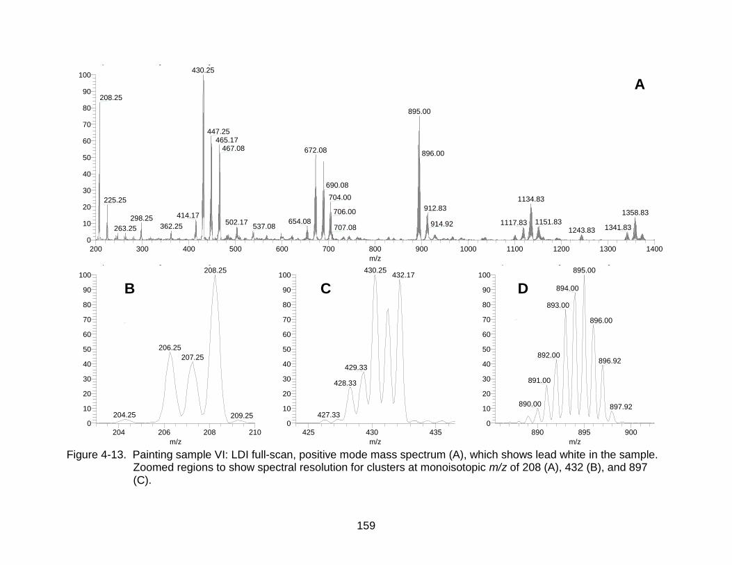
159
Figure 4-13. Painting sample VI: LDI full-scan, positive mode mass spectrum (A), which shows lead white in the sample. Zoomed regions to show spectral resolution for clusters at monoisotopic m/z of 208 (A), 432 (B), and 897 (C).
F_surface_TI #194-241 RT: 4.77-5.97 AV: 48 NL: 6.34E3T: ITMS + p MALDI Full ms [50.00-2000.00]
200 300 400 500 600 700 800 900 1000 1100 1200 1300 1400
m/z
0
10
20
30
40
50
60
70
80
90
100
Rela
tive A
bundance
430.25
208.25
895.00
447.25465.17
467.08 672.08 896.00
690.08
704.00 1134.83225.25912.83
706.00 1358.83414.17298.25 654.08 1151.83502.17 1117.83914.92362.25 537.08 1341.83707.08263.25 1243.83
F_surface_TI #194-241 RT: 4.77-5.97 AV: 48 NL:T: ITMS + p MALDI Full ms [50.00-2000.00]
204 206 208 210
m/z
0
10
20
30
40
50
60
70
80
90
100
Re
lative
Ab
un
da
nce
208.25
206.25
207.25
204.25 209.25
F_surface_TI #194-241 RT: 4.77-5.97 AV: 48 NL:T: ITMS + p MALDI Full ms [50.00-2000.00]
425 430 435
m/z
0
10
20
30
40
50
60
70
80
90
100
Re
lative
Ab
un
da
nce
430.25432.17
429.33
428.33
427.33
F_surface_TI #194-241 RT: 4.77-5.97 AV: 48 NL:T: ITMS + p MALDI Full ms [50.00-2000.00]
890 895 900
m/z
0
10
20
30
40
50
60
70
80
90
100
Re
lative
Ab
un
da
nce
895.00
894.00
893.00
896.00
892.00896.92
891.00
890.00 897.92
A
B C D
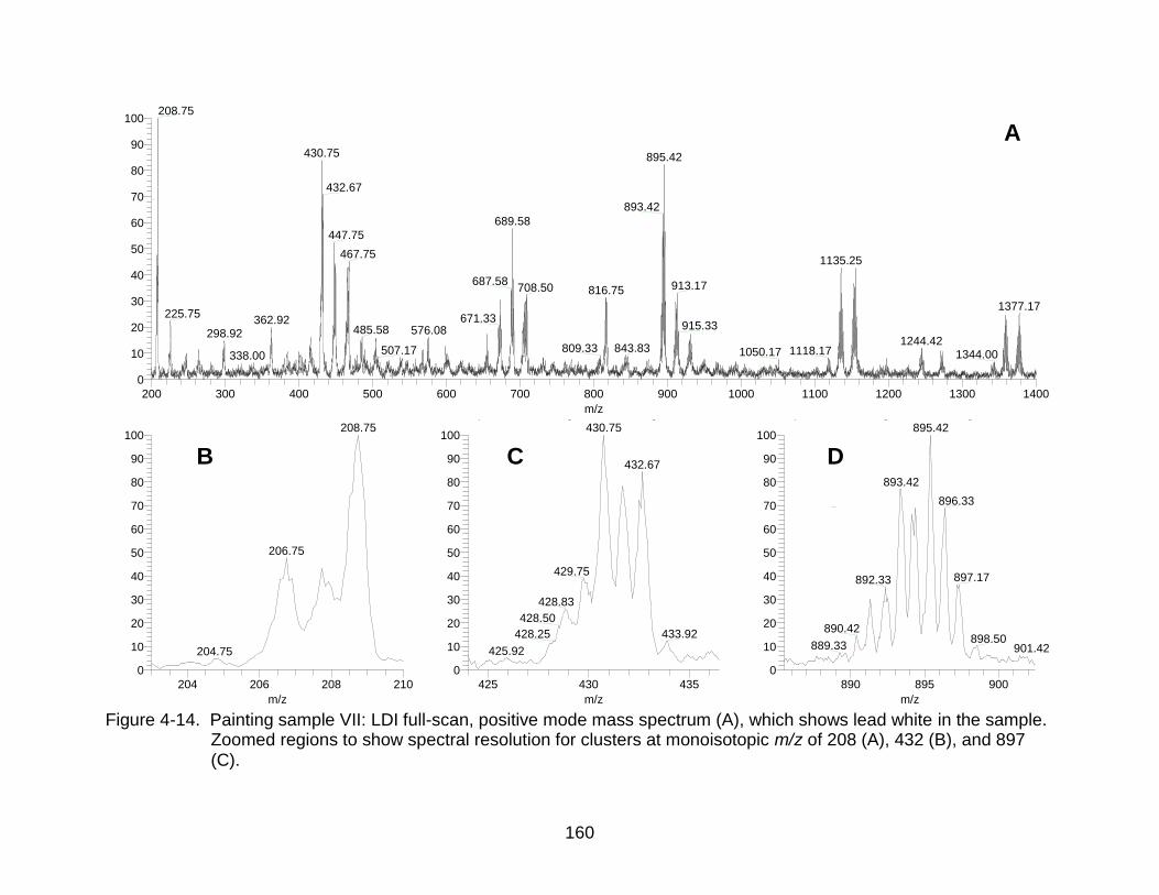
160
Figure 4-14. Painting sample VII: LDI full-scan, positive mode mass spectrum (A), which shows lead white in the sample. Zoomed regions to show spectral resolution for clusters at monoisotopic m/z of 208 (A), 432 (B), and 897 (C).
Hagain_TI #69 RT: 1.09 AV: 1 NL: 8.26E3T: ITMS + p MALDI Full ms [150.00-2000.00]
200 300 400 500 600 700 800 900 1000 1100 1200 1300 1400
m/z
0
10
20
30
40
50
60
70
80
90
100
Rela
tive A
bundance
208.75
430.75 895.42
432.67
893.42
689.58
447.75
467.751135.25
687.58 913.17708.50 816.75
1377.17225.75 671.33362.92
915.33485.58 576.08298.921244.42
843.83809.33507.17 1118.171050.17 1344.00338.00
Hagain_TI #69 RT: 1.09 AV: 1 NL: 8.26E3T: ITMS + p MALDI Full ms [150.00-2000.00]
204 206 208 210
m/z
0
10
20
30
40
50
60
70
80
90
100
Re
lative
Ab
un
da
nce
208.75
206.75
204.75
Hagain_TI #69 RT: 1.09 AV: 1 NL: 6.93E3T: ITMS + p MALDI Full ms [150.00-2000.00]
425 430 435
m/z
0
10
20
30
40
50
60
70
80
90
100
Re
lative
Ab
un
da
nce
430.75
432.67
429.75
428.83
428.50
433.92428.25
425.92
Hagain_TI #69 RT: 1.09 AV: 1 NL: 6.80E3T: ITMS + p MALDI Full ms [150.00-2000.00]
890 895 900
m/z
0
10
20
30
40
50
60
70
80
90
100
Re
lative
Ab
un
da
nce
895.42
893.42
896.33
897.17892.33
890.42898.50
889.33 901.42
A
B C D
161
CHAPTER 5 CONCLUSION AND FUTURE DIRECTIONS
Conclusions
The preservation of cultural heritage is of critical importance to the continuance
of a people, their connection to their past, their outlook toward their future, and their
pride, celebration, and enjoyment thereof. The spectacularly rich and voluminous
amount of art created over millennia is resoundingly worthy of the efforts engaged
toward its preservation. Over the past few decades, scientists—particularly analytical
chemists—and conservation scientists have applied and, to a lesser extent, developed
state-of-the-art analytical technologies for the analyses of artistic and archaeological
objects for such purposes as component detection, dating, provenance, and taphonomy
with the ultimate goals of restoration and preservation (viz., conservation). Thus, the
underlying philosophy of this dissertation was to utilize scientific positivistic, empirical,
and experimental approaches to further strengthen the union of analytical chemistry—
particularly mass spectrometry—to the field of conservation science.
The practical goal of the research presented in this dissertation was to develop
and employ laser desorption/ionization-tandem mass spectrometric techniques
(LDI-MS/MS) in the analysis of the dye madder—particularly the anthraquinones alizarin
and purpurin—and the pigment lead white in fragments of paintings and swatches of
dyed silk. To achieve that goal, neat standards of selected anthraquinones and lead
white were initially tested with LDI-MS and LDI-MS/MS to observe their ionization and
fragmentation behavior and to elucidate the structure of the ions formed, and then those
data were applied to the detection of those colorants in real samples.
162
In the analyses of the anthraquinones, the peculiar ionization that formed
anomalous [M+2H] •+ ions was fully explored with LDI-MS/MS for the first time. The
results show that anthraquinones exhibit laser-induced reduction about the carbonyl
central to the anthracene skeleton, observed as the neutral loss of 29 (COH) with the
concomitant decrease in neutral losses of 28 (CO) and 56 (2CO). Furthermore,
differences in fragmentation were exhibited for anthraquinones with functional groups
(e.g., hydroxyl or amine) proximal to the reduced carbonyl versus anthraquinones with
those groups distal to the reduced carbonyl. These results, new to LDI mass
spectrometry, stand to benefit the conservation science community by alerting them to
the presence and correct interpretation of otherwise unexpected ionization of this
important class of compounds in artistic dyes.
The ubiquitous pigment lead white was analyzed by LDI-MS/MS and
LDI-Orbitrap-MS/MS for the first time. The distinct pattern of superclusters, capital
clusters, and miniscule clusters makes the observation of the pigment relatively simple
and quick. Through deductive and inductive reasoning, the formulae of the majority of
clusters was determined via the superior spectral resolving power and mass accuracy of
the Orbitrap for ions observed in both the full and daughter-ion scans. Exploiting the
distinctive isotopic pattern of lead to match isotopic patterns between experimental and
theoretical spectra, the full-scan spectrum was first divided into superclusters based
upon the number of lead atoms. The isotopic pattern of lead was subsequently used to
identify the monoisotopic mass of each cluster, from which a lead-limited, accurate
formula could be derived. Formulae that remained indeterminate were inductively
determined using tandem mass spectra and pattern matching to the already-determined
163
formulae. These methods, completely new to mass spectrometry, can benefit the
communities of mass spectrometrists and conservation scientists by offering a new
method of interpretation of isotopically complex cluster ions of a pigment ubiquitous
since antiquity.
Lastly, the preceding methodologies were applied to the in situ detection of
madder and lead white in “real” samples, including fragments of paintings and swatches
of dyed silk. Two components of the red dye madder, alizarin and purpurin, were
detected in their reduced and unreduced forms using tandem mass spectrometry,
despite their not being present at detectable levels in the full-scan spectra. The pigment
lead white was easily detected in painting fraqments using only full-scan spectra despite
the presence of wax or varnish atop the paint layer. The successful in situ LDI-MS/MS
analysis of alizarin and purpurin and LDI-MS analysis of lead white were the first
instances ever documented for fragments of paintings or swatches of dyed silk, and
both were accomplished without any sample pretreatment whatsoever.
Overall, the results obtained and conclusions drawn are not a dramatic leap
forward for science as a whole, but they do represent a significant step forward for the
relatively young and burgeoning field of conservation science. Therefore, it is
recommended that the material presented in this dissertation be disseminated
throughout the community.
Future Directions
Though the work presented in this dissertation includes well-researched literature
reviews, complete experiments, and definitive conclusions, there exist several aspects
open to further exploration and experimentation. These future directions can neither
negate nor supplant the findings presented here, they may only bolster the findings.
164
Although the laser-induced reduction of anthraquinones was definitively proven
by the appearance of the [M+2H] •+ ion, neutral loss of a reduced carbonyl, and
decrease in the relative abundance of the neutral loss of one and two carbonyls, there
are still three sets of experiments that should be conducted. First, anthraquinones that
are deliberately exposed to UV light in a controlled environment should be analyzed
with electrospray ionization tandem mass spectrometry. The anthraquinone that was
analyzed was only unintentionally exposed to UV after not having been stored in a
darkened container over several days. A controlled time-course study of UV exposure
may reveal a dependence on the abundance of P+1 relative to P, which may provide
further insight to the underlying physiochemical process of photon-induced reduction.
Second, many more experiments could be devised and conducted to control the many
variables influencing LDI in the source chamber. These variables include, but are not
limited to, source pressure, partial pressure of water, temperature, surface substrate,
and the use of electron-capturing additives. Third, to test the influence of UV photons
on the laser-induced reduction, a laser that delivers IR photons, such as a CO2 laser
( ≈ 10 μm), should be used, rather than the N2 laser, which delivers UV photons
( = 337 nm).
The analysis of lead white is novel not only because of the elucidation of the
clusters themselves, but because of the limited precedent in the literature of deciphering
isotopically complex middle molecules. To improve the elucidation of all isotopically
complex middle molecules—not just lead white—experiments exercising
thermodynamic control at the ionization source and kinetic control at the ion trap are
proposed, though lead white will be discussed as the exemplar case.
165
Thermodynamically controlled experiments at the ionization source are intended to
observe changes, if any, in the presence and relative intensity of clusters and should
include variables such as source pressure and laser fluence. Indeed, the quality of the
lead white spectra was negatively affected by high laser energies, since the pigment
has a very low ionization threshold and produces significant signal at a very low laser
energy. The analysis presented was focused on elucidating the clusters in clean,
low-noise spectra—a challenge in itself—and not did not venture in to creating even
more complex spectra at higher laser power. Kinetic control at the ion trap should
include varying the activation time with and without a change in the value of
collision-activated dissociation (CID). Since cluster formation may occur in the gas
phase after ionization, varying activation time—particularly with zero CID—may produce
different clusters in full-scan or daughter-ion spectra. This dependence on residence
time within the mass spectrometer may have already been observed in Figure 3-6,
which shows different daughter-ion clusters from the same precursor cluster using the
ion trap and Orbitrap, the latter of which necessitates a much longer ion transport as an
ion travels from the LIT to the Orbitrap.
Lastly, analysis of real art samples might be improved and expanded upon by
altering or examining the samples’ surface. The samples tested had no pretreatment
other than the use of double-sided tape to adhere them to the sample plate. However,
the surface of the fragments of paintings could have been cleaned with solvent to
remove the wax or varnish or other surface chemicals and contaminants to promote
interaction of the laser’s UV photons with the dyes and/or pigments in the paint layer.
Moreover, the laser itself may have been used, such as with the instrument’s “sweep
166
shot” setting to ablate a top layer from the sample as a pseudo “cleaning” process. One
objective of a conservation scientist is to have a totally non-invasive analytical
technique. Considering that LDI is a non-destructive process, it will be useful to gather
some information as to the extent of its destruction of the surface. This information can
be obtained via visible light microscopy or scanning electron microscopy, depending on
the level of resolution desired, before and after LDI analysis. Other future directions for
real samples might be dictated as needed simply by the types of sample and analysis at
hand.
167
REFERENCES
(1) UN UNESCO World Heritage Centre - Convention Concerning the Protection of the World Cultural and Natural Heritage. http://whc.unesco.org/?cid=175 (accessed April 2013)
(2) Ciliberto, E.; Spoto, G. Modern analytical methods in art and archaeology; Wiley: New York, 2000.
(3) Artioli, G. Scientific Methods and Cultural Heritage: An introduction to the application of materials science to archaeometry and conservation science; OUP Oxford: Oxford, 2010.
(4) Pollard, A. M.; Heron, C. Archaeological Chemistry; Royal Society of Chemistry: Cambridge, 2008.
(5) Caley, E. R. J. Chem. Educ. 1951, 28, 64-66.
(6) Fremout, W.; Saverwyns, S.; Peters, F.; Deneffe, D. J. Raman Spectrosc. 2006, 37, 1035-1045.
(7) Andrikopoulos, K. S.; Daniilia, S.; Roussel, B.; Janssens, K. J. Raman Spectrosc. 2006, 37, 1026-1034.
(8) Dussubieux, L.; Robertshaw, P.; Glascock, M. D. Int. J. Mass Spectrom. 2009, 284, 152-161.
(9) Tognazzi, A.; Dattilo, A. M.; Bracchini, L.; Aggravi, M.; Benetti, F.; Mugnaini, E.; Magnani, A.; Rossi, C. Surf. Interface Anal. 2011, 43, 1108-1119.
(10) Niimura, N. Int. J. Mass Spectrom. 2009, 284, 93-97.
(11) Oudemans, T. F. M.; Eijkel, G. B.; Boon, J. J. J. Archaeol. Sci. 2007, 34, 173-193.
(12) Honig, R. E.; Woolston, J. R. Appl. Phys. Lett. 1963, 2, 138-139.
(13) Fenner, N. C.; Daly, N. R. Rev. Sci. Instrum. 1966, 37, 1068-1070.
(14) Denoyer, E.; van Grieken, R.; Adams, F.; Natusch, D. F. S. Anal. Chem. 1982, 54, 26A-41A.
(15) Vastola, F. J.; Mumma, R. O.; Pirone, A. J. Org. Mass Spectrom. 1970, 3, 101-104.
(16) Hillenkamp, F.; UnsoLd, E.; Kaufmann, R.; Nitsche, R. Nature 1975, 256, 119-120.
(17) Hillenkamp, F.; Peter-Katalinic, J. MALDI MS; Wiley-VCH: Weinheim, 2007.
168
(18) Aberth, W.; Straub, K. M.; Burlingame, A. L. Anal. Chem. 1982, 54, 2029-2034.
(19) Beckey, H. D. Int. J. Mass Spectrom. Ion Phys. 1969, 2, 500-502.
(20) Torgerson, D. F.; Skowronski, R. P.; Macfarlane, R. D. Biochem. Biophys. Res. Commun. 1974, 60, 616-621.
(21) Benninghoven, A.; Sichtermann, W. K. Anal. Chem. 1978, 50, 1180-1184.
(22) Barber, M.; Bordoli, R. S.; Sedgwick, R. D.; Tyler, A. N. J. Chem. Soc., Chem. Commun. 1981, 0, 325-327.
(23) Liao, P. C.; Allison, J. J. Mass Spectrom. 1995, 30, 408-423.
(24) Bourcier, S.; Bouchonnet, S.; Hoppilliard, Y. Int. J. Mass Spectrom. 2001, 210/211, 59-69.
(25) Karbach, V.; Knochenmuss, R.; Zenobi, R. Rapid Commun. Mass Spectrom. 1998, 12.
(26) Karas, M.; Bachmann, D.; Hillenkamp, F. Anal. Chem. 1985, 57.
(27) Fenn, J. B.; Mann, M.; Meng, C. K.; Wong, S. F.; Whitehouse, C. M. Science 1989, 246, 64-71.
(28) Watson, J. T. Introduction to Mass Spectrometry, Third ed.; Lippincott-Raven: New York, NY, 1997.
(29) Watson, J. T.; Sparkman, O. D. Introduction to Mass Spectrometry: Instrumentation, Applications, and Strategies for Data Interpretation; Wiley: West Sussex, 2008.
(30) Cech, N. B.; Enke, C. G. Mass Spectrom. Rev. 2001, 20, 362-387.
(31) Gomez, A.; Tang, K. Phys. Fluids 1994, 6, 404-414.
(32) Cole, R. B. J. Mass Spectrom. 2000, 35, 763-772.
(33) Dole, M.; Mack, L. L.; Hines, R. L.; Mobley, R. C.; Ferguson, L. D.; Alice, M. B. J. Chem. Phys. 1968, 49, 2240-2249.
(34) Iribarne, J. V.; Thomson, B. A. J. Chem. Phys. 1976, 64, 2287-2294.
(35) Nobel The Nobel Prize in Physics 1989. http://nobelprize.org/nobel_prizes/physics/laureates/1989/index.html (accessed May 2013)
(36) Schwartz, J. C.; Senko, M. W.; Syka, J. E. P. J. Am. Soc. Mass Spectrom. 2002, 13, 659-669.
169
(37) Blackler, A. R.; Klammer, A. A.; MacCoss, M. J.; Wu, C. C. Anal. Chem. 2006, 78, 1337-1344.
(38) March, R. E. J. Mass Spectrom. 1997, 32, 351-369.
(39) Julian, R. K.; Cooks, R. G. Anal. Chem. 1993, 65, 1827-1833.
(40) Guan, S.; Marshall, A. G. Anal. Chem. 1993, 65, 1288-1294.
(41) Louris, J. N.; Taylor, D. M. Method and apparatus for ejecting unwanted ions in an ion trap mass spectrometer. U.S. Patent 5,324,939, 1994.
(42) Hu, Q.; Noll, R. J.; Li, H.; Makarov, A.; Hardman, M.; Graham Cooks, R. J. Mass Spectrom. 2005, 40, 430-443.
(43) Hardman, M.; Makarov, A. A. Anal. Chem. 2003, 75, 1699-1705.
(44) Makarov, A.; Denisov, E.; Kholomeev, A.; Balschun, W.; Lange, O.; Strupat, K.; Horning, S. Anal. Chem. 2006, 78, 2113-2120.
(45) Strupat, K.; Kovtoun, V.; Bui, H.; Viner, R.; Stafford, G.; Horning, S. J. Am. Soc. Mass Spectrom. 2009, 20, 1451-1463.
(46) Scigelova, M.; Makarov, A. Proteomics 2006, 6, 16-21.
(47) Perry, R. H.; Cooks, R. G.; Noll, R. J. Mass Spectrom. Rev. 2008, 27, 661-699.
(48) Olsen, J. V.; de Godoy, L. M. F.; Li, G.; Macek, B.; Mortensen, P.; Pesch, R.; Makarov, A.; Lange, O.; Horning, S.; Mann, M. Mol. Cell. Proteomics 2005, 4, 2010-2021.
(49) Xian, F.; Hendrickson, C. L.; Marshall, A. G. Anal. Chem. 2012, 84, 708-719.
(50) Roy, A. Artists' Pigments: A Handbook of Their History and Characteristics; Cambridge University Press: Cambridge 1993.
(51) Zollinger, H. Color Chemistry: Syntheses, Properties, and Applications of Organic Dyes and Pigments; Wiley-VCH: Weinheim, 2004.
(52) de Graaff, J. H. H.; Roelofs, W. G. T.; van Bommel, M. R. The colourful past: origins, chemistry and identification of natural dyestuffs; Archetype: London, 2004.
(53) Mills, J. S.; White, R. The Organic Chemistry of Museum Objects, 2 ed.; Butterworth-Heinemann, 1994.
(54) Mouri, C.; Laursen, R. Microchim. Acta 2012, 179, 105-113.
170
(55) Derksen, G. C. H.; Van Beek, T. A.; Atta-ur, R. In Studies in Natural Products Chemistry; Elsevier, 2002; Vol. 26, Part G, pp 629-684.
(56) Saunders, D.; Kirby, J. Nat. Gall. Tech. Bull. 1994, 15, 79-97.
(57) Thomson, R. H. Naturally Occurring Quinones, 2nd ed.; Academic Press: New York, 1971.
(58) Graebe, C.; Liebermann, C. Chem. Ber. 1869, 2, 332.
(59) Gordon, P. F.; Gregory, P. Organic Chemistry in Colour; Springer: New York, 1983.
(60) Puchalska, M.; Orlinska, M.; Ackacha, M. A.; Potec-Pawlak, K.; Jarosz, M. J. Mass Spectrom. 2003, 38, 1252-1258.
(61) Wouters, J.; Rosario-Chirinos, N. J. Am. Instit. Conserv. 1992, 31, 237-255.
(62) Boldizsar, I.; Szucs, Z.; Fuzfai, Z.; Molnar-Perl, I. J. Chromatogr. A 2006, 1133, 259-274.
(63) Ackacha, M. A.; Potec-Pawlak, K.; Jarosz, M. J. Sep. Sci. 2003, 26, 1028-1034.
(64) Degano, I.; Ribechini, E.; Modugno, F.; Colombini, M. P. Appl. Spectrosc. Rev. 2009, 44, 363-410.
(65) Derksen, G. C. H.; Neiderlander, H. A. G.; van Beek, T. A. J. Chromatogr. A 2002, 978, 119-127.
(66) Ahn, C.; Obendorf, S. K. Text. Res. J. 2004, 74, 949-954.
(67) Shibayama, N.; Yamaoka, R.; Sato, M. Analysis of Colored Compounds found in Natural Dyes by Thermospray Liquid Chromatography-Mass Spectrometry (TSP LC-MS) and a Preliminary Study of the Application to Analysis of Natural Dyes used on Historic Textiles. Instituut Collectie Nederland, Dyes in History and Archaeology 20, Amsterdam, The Netherlands 2001; Archetype Publications; 51-69.
(68) Surowiec, I.; Szostek, B.; Trojanowicz, M. J. Sep. Sci. 2007, 30, 2070-2079.
(69) Szostek, B.; Orska-Gawrys, J.; Surowiec, I.; Trojanowicz, M. J. Chromatogr. A 2003, 1012, 179-192.
(70) Epolito, W. J.; Lee, Y. H.; Bottomley, L. A.; Pavlostathis, S. G. Dyes Pigm. 2005, 67, 35-46.
(71) DeRoo, C. S.; Armitage, R. A. Anal. Chem. 2011, 83, 6924-6928.
171
(72) Bennett, J. A.; Schweikert, E. A.; van Vaeck, L.; Adams, F. C. J. Trace Microprobe Tech. 1990, 7, 279-292.
(73) Dale, M. J.; Jones, A. C.; Langridge-Smith, P. R. R.; Costello, K. F.; Cummins, P. G. Anal. Chem. 1993, 65, 793-801.
(74) Grim, D. M. Dissertation, Michigan State University, 2003.
(75) Grim, D. M.; Allison, J. Int. J. Mass Spectrom. 2003, 222, 85-99.
(76) Grim, D. M.; Allison, J. Archaeometry 2004, 46, 283-299.
(77) Wyplosz, N. Dissertation, FOM-Institute for Atomic and Molecular Physics, Amsterdam, 2003.
(78) Soltzberg, L. J.; Hagar, A.; Kridaratikorn, S.; Mattson, A.; Newman, R. J. Am. Soc. Mass Spectrom. 2007, 18, 2001-2006.
(79) Van Elslande, E.; Guérineau, V.; Thirioux, V.; Richard, G.; Richardin, P.; Laprévote, O.; Hussler, G.; Walter, P. Anal. Bioanal. Chem. 2008, 390, 1873-1879.
(80) Kirby, D. P.; Khandekar, N.; Sutherland, K.; Price, B. A. Int. J. Mass Spectrom. 2009, 284, 115-122.
(81) Lou, X.; Sinkeldam, R. W.; van Houts, W.; Nicolas, Y.; Janssen, P. G. A.; van Dongen, J. L. J.; Vekemans, J. A. J. M.; Meijer, E. W. J. Mass Spectrom. 2007, 42, 293-303.
(82) Meijer, W. W. prof.dr. E.W. (Bert) Meijer - Expertises. http://www.tue.nl/en/employee/ep/e/d/ep-uid/19911632 (accessed November 1, 2012)
(83) Karas, M.; Glückmann, M.; Schäfer, J. J. Mass Spectrom. 2000, 35, 1-12.
(84) Frankevich, V.; Knochenmuss, R.; Zenobi, R. Int. J. Mass Spectrom. 2002, 220, 11-19.
(85) Frankevich, V. E.; Zhang, J.; Friess, S. D.; Dashtiev, M.; Zenobi, R. Anal. Chem. 2003, 75, 6063-6067.
(86) Zhang, J.; Frankevich, V.; Knochenmuss, R.; Friess, S. D.; Zenobi, R. J. Am. Soc. Mass Spectrom. 2003, 14, 42-50.
(87) Okuno, S.; Nakano, M.; Matsubayashi, G.-e.; Arakawa, R.; Wada, Y. Rapid Commun. Mass Spectrom. 2004, 18, 2811-2817.
172
(88) Kosevich, M. V.; Chagovets, V. V.; Shmigol, I. V.; Snegir, S. V.; Boryak, O. A.; Orlov, V. V.; Shelkovsky, V. S.; Pokrovskiy, V. A.; Gomory, A. J. Mass Spectrom. 2008, 43, 1402-1412.
(89) McAvey, K. M.; Guan, B.; Fortier, C. A.; Tarr, M. A.; Cole, R. B. J. Am. Soc. Mass Spectrom. 2011, 22, 659-669.
(90) Aplin, R. T.; Pike, W. T. Chem. Ind. (London) 1966, 2009.
(91) Ukai, S.; Hirose, K.; Tatematsu, A.; Goto, T. Tetrahedron Lett. 1967, 8, 4999-5002.
(92) Cornforth, J. W.; Ryback, G.; Robinson, P. M.; Park, D. J. Chem. Soc. C: Org. 1971, 2786-2788.
(93) Oliver, R. W. A.; Rashman, R. M. J. Chem. Soc. B: Phys. Org. 1968, 1141-1143.
(94) Oliver, R. W. A.; Rashman, R. M. J. Chem. Soc. B: Phys. Org. 1971, 341-344.
(95) Grigsby, R. D.; Jamieson, W. D.; McInnes, A. G.; Maass, W. S. G.; Taylor, A. Can. J. Chem. 1974, 52, 4117-4122.
(96) Beaumont, P. C.; Edwards, R. L. J. Chem. Soc. C: Org. 1969, 2398-2403.
(97) Gaylord, M. C.; Brady, L. R. J. Pharm. Sci. 1971, 60, 1503-1508.
(98) Das, B. C.; Lounasmaa, M.; Tendille, C.; Lederer, E. Biochem. Biophys. Res. Commun. 1965, 21, 318-322.
(99) Patai, S.; Rappoport, Z. The Chemistry of the Quinonoid Compounds; John Wiley & Sons: New York, 1974.
(100) Fessenden, R. J.; Fessenden, J. S.; Feist, P. Organic Laboratory Techniques; Brooks/Cole: Pacific Grove, 2001.
(101) Karas, M.; Hillenkamp, F. Anal. Chem. 1988, 60, 2299-2301.
(102) de la Mora, J. F.; Van Berkel, G. J.; Enke, C. G.; Cole, R. B.; Martinez-Sanchez, M.; Fenn, J. B. J. Mass Spectrom. 2000, 35, 939-952.
(103) Beynon, J. H.; Williams, A. E. Appl. Spectrosc. 1960, 14, 156-160.
(104) Bowie, J. H.; Cameron, D. W.; Giles, R. G. F.; Williams, D. H. J. Chem. Soc. B: Phys. Org. 1966, 335-339.
(105) Filyugina, A. D.; Kolokolov, B. N.; Bragina, S. I.; Rotermel, I. A.; Dubrovia, A. A. Russ. J. Org. Chem. 1972, 8, 2151-2155.
173
(106) Vasileva, A. D.; Rotermel, I. A.; Artamonova, N. N.; Gaeva, L. A.; Dubrovia, A. A.; Kolokolov, B. N. Russ. J. Org. Chem. 1972, 8, 2156-2159.
(107) Proctor, C. J.; Kralj, B.; Larka, E. A.; Porter, C. J.; Maquestiau, A.; Beynon, J. H. Org. Mass Spectrom. 1981, 16, 312-322.
(108) Pan, Y.; Zhang, L.; Zhang, T.; Guo, H.; Hong, X.; Qi, F. J. Mass Spectrom. 2008, 43, 1701-1710.
(109) Patai, S.; Rappoport, Z. The Chemistry of the Quinonoid Compounds; John Wiley & Sons: New York, 1988.
(110) Carlson, S. A.; Hercules, D. M. Photochem. Photobiol. 1973, 17, 123-131.
(111) Carlson, S. A.; Hercules, D. M. Anal. Chem. 1973, 45, 1794-1799.
(112) Gorner, H. Photochem. Photobiol. 2003, 77, 171-179.
(113) Tickle, K.; Wilkinson, F. Trans. Faraday Soc. 1965, 61, 1981-1990.
(114) Wakisaka, A.; Ebbesen, T. W.; Sakuragi, H.; Tokumaru, K. J. Phys. Chem. 1987, 91, 6547-6551.
(115) Flom, S. R.; Barbara, P. F. J. Phys. Chem. 1985, 89, 4489-4494.
(116) Gollnick, K.; Held, S.; Mártire, D. O.; Braslavsky, S. E. J. Photochem. Photobiol., A 1992, 69, 155-165.
(117) Young, W. J. Application of Science in Examination of Works of Art: Proceedings of the Seminar: June 15-19, 1970; Museum of Fine Arts: Boston, 1973.
(118) De Wannemacker, G.; Vanhaecke, F.; Moens, L.; Van Mele, A.; Thoen, H. J. Anal. At. Spectrom. 2000, 15, 323-327.
(119) Schultheis, G.; Prohaska, T.; Stingeder, G.; Dietrich, K.; Jembrih-Simburger, D.; Schreiner, M. J. Anal. At. Spectrom. 2004, 19, 838-843.
(120) Fortunato, G.; Ritter, A.; Fabian, D. Analyst 2005, 130, 898-906.
(121) De Laeter, J.; Kurz, M. D. J. Mass Spectrom. 2006, 41, 847-854.
(122) Keisch, B.; Callahan, R. C. Archaeometry 1976, 18, 181-193.
(123) Van Elslande, E.; Guerineau, V.; Thirioux, V.; Richard, G.; Richardin, P.; Laprevote, O.; Hussler, G.; Walter, P. Anal. Bioanal. Chem. 2008, 390, 1873-1879.
(124) de Heer, W. A. Rev. Mod. Phys. 1993, 65, 611-676.
174
(125) Mühlbach, J.; Sattler, K.; Pfau, P.; Recknagel, E. Phys. Lett. A 1982, 87, 415-417.
(126) Hoareau, A.; Mélinon, P.; Cabaud, B.; Rayane, D.; Tribollet, B.; Broyer, M. Chem. Phys. Lett. 1988, 143, 602-608.
(127) Dean, L. K. L.; Didonato, G. C.; Busch, K. L. Inorg. Chim. Acta 1989, 157, 175-185.
(128) Katakuse, I.; Ichihara, T.; Ito, H.; Matsuo, T.; Sakurai, T.; Matsuda, H. Int. J. Mass Spectrom. Ion Processes 1989, 91, 93-97.
(129) Xing, X.; Tian, Z.; Liu, H.; Tang, Z. Rapid Commun. Mass Spectrom. 2003, 17, 1411-1415.
(130) Waldschmidt, B.; Barman, S.; Rajesh, C.; Majumder, C.; Das, G. P.; Schäfer, R. Phys. Rev. B 2009, 79, 045422.
(131) Prussakowska, M.; Sokalska, M.; Gierczyk, B.; Kozik, T.; Frański, R. Rapid Commun. Mass Spectrom. 2010, 24, 1925-1929.
(132) Kelting, R.; Otterstatter, R.; Weis, P.; Drebov, N.; Ahlrichs, R.; Kappes, M. M. J. Chem. Phys. 2011, 134, 024311.
(133) Echt, O.; Sattler, K.; Recknagel, E. Phys. Rev. Lett. 1981, 47, 1121-1124.
(134) Dyson, P.; McGrady, J.; Reinhold, M.; Johnson, B. G.; McIndoe, J. S.; Langridge-Smith, P. R. J. Cluster Sci. 2000, 11, 391-401.
(135) Fenselau, C. Anal. Chem. 1982, 54, 105A-116A.
(136) Brack, M. Rev. Mod. Phys. 1993, 65, 677-732.
(137) Scheidegger, C.; Suter, M. J. F.; Behra, R.; Sigg, L. Front. Microbiol. 2012, 3.
(138) Fenselau, C.; Cotter, R.; Hansen, G.; Chen, T.; Heller, D. J. Chrom. A 1981, 218, 21-30.
(139) Yergey, J.; Heller, D.; Hansen, G.; Cotter, R. J.; Fenselau, C. Anal. Chem. 1983, 55, 353-356.
(140) Senko, M. W.; Beu, S. C.; McLafferty, F. W. J. Am. Soc. Mass Spectrom. 1995, 6, 229-233.
(141) O'Connor, P. B.; Little, D. P.; McLafferty, F. W. Anal. Chem. 1996, 68, 542-545.
(142) Valkenborg, D.; Mertens, I.; Lemière, F.; Witters, E.; Burzykowski, T. Mass Spectrom. Rev. 2012, 31, 96-109.
175
(143) Yergey, J. A. Int. J. Mass Spectrom. Ion Phys. 1983, 52, 337-349.
(144) McLafferty, F. W.; Tureček, F. Interpretation of Mass Spectra, 4th ed.; Univ. Science Books: Mill Valley, 1993.
(145) Yamamoto, H.; McCloskey, J. A. Anal. Chem. 1977, 49, 281-283.
(146) Hibbert, D. B. Chemom. Intell. Lab. Syst. 1989, 6, 203-212.
(147) Rosman, K. J. R.; Taylor, P. D. P. 4th International Symposium on Bioorganic Chemistry 1997, 70, 217-235.
(148) Rockwood, A. L. Rapid Commun. Mass Spectrom. 1997, 11, 241-248.
(149) Rockwood, A.; Kushnir, M.; Nelson, G. J. Am. Soc. Mass Spectrom. 2003, 14, 311-322.
(150) Bozorgzadeh, M. H.; Morgan, R. P.; Beynon, J. H. Analyst 1978, 103, 613-622.
(151) Todd, P. J.; Barbalas, M. P.; McLafferty, F. W. Org. Mass Spectrom. 1982, 17, 79-80.
(152) Singleton, K. E.; Cooks, R. G.; Wood, K. V. Anal. Chem. 1983, 55, 762-764.
(153) Bozorgzadeh, M. H. Rapid Commun. Mass Spectrom. 1988, 2, 61-64.
(154) de Hoffman, E.; Auriel, M. Org. Mass Spectrom. 1989, 24, 748-758.
(155) Glish, G.; McLuckey, S.; Asano, K. J. Am. Soc. Mass Spectrom. 1990, 1, 166-173.
(156) Cataldi, T. R. I.; Lelario, F.; Orlando, D.; Bufo, S. A. Anal. Chem. 2010, 82, 5686-5696.
(157) Tou, J. C. Anal. Chem. 1983, 55, 367-372.
(158) Bozorgzadeh, M. H.; Lapp, R. L.; Gross, M. L. Org. Mass Spectrom. 1988, 23, 712-718.
(159) Elslande, E.; Guérineau, V.; Thirioux, V.; Richard, G.; Richardin, P.; Laprévote, O.; Hussler, G.; Walter, P. Anal. Bioanal. Chem. 2008, 390, 1873-1879.
(160) Reich, R. F.; Cudzilo, K.; Levisky, J. A.; Yost, R. A. J. Am. Soc. Mass Spectrom. 2010, 21, 564-571.
(161) Critchley, G.; Dyson, P. J.; Johnson, B. F. G.; McIndoe, J. S.; O'Reilly, R. K.; Langridge-Smith, P. R. R. Organometallics 1999, 18, 4090-4097.
176
(162) Colombini, P. M. P.; Modugno, F. Organic Mass Spectrometry in Art and Archaeology; John Wiley & Sons: West Sussex, 2009.
(163) Glascock, M. D.; Speakman, R. J.; Popelka-Filcoff, R. S. Archaelogical Chemistry #968: Analytical Techniques and Archaeological Interpretation; OUP USA: Washington, DC, 2007.
(164) Mazel, V.; Richardin, P.; Touboul, D.; Brunelle, A.; Walter, P.; Laprévote, O. Anal. Chim. Acta 2006, 570, 34-40.
(165) Keune, K. Dissertation, FOM-Institute for Atomic and Molecular Physics, Amsterdam, 2005.
(166) Keune, K.; Boon, J. J. Anal. Chem. 2004, 76, 1374-1385.
(167) Keune, K.; Boon, J. J. Anal. Chem. 2005, 77, 4742-4750.
(168) Keune, K.; Hoogland, F.; Boon, J. J.; Peggie, D.; Higgitt, C. Int. J. Mass Spectrom. 2009, 284, 22-34.
(169) Sanyova, J.; Cersoy, S.; Richardin, P.; Laprévote, O.; Walter, P.; Brunelle, A. Anal. Chem. 2011, 83, 753-760.
(170) Richardin, P.; Mazel, V.; Walter, P.; Laprévote, O.; Brunelle, A. J. Am. Soc. Mass Spectrom. 2011, 22, 1729-1736.
(171) Kuckova, S.; Nemec, I.; Hynek, R.; Hradilova, J.; Grygar, T. Anal. Bioanal. Chem. 2005, 382, 275-282.
177
BIOGRAPHICAL SKETCH
Michael (Mike) Patrick Napolitano was born and raised in Rahway, New Jersey.
Both his father, whom emigrated alone from Italy and without a command of English,
and mother, she a child of immigrants, instilled in him the value of higher education and
the idea of the American Dream while holding true the virtues of both the Catholic
Church and the Occident. To that effect, Michael attended twelve years of Catholic
grammar and high school, and then earned his ACS-certified Bachelor of Science in
chemistry from the Pennsylvania State University in 2003. During his time at Penn
State, he was a research assistant in the mass spectrometry research laboratory of
Dr. A. Daniel Jones. Following graduation, Michael first traveled to Europe where, for
the first time, he met many of his relatives in Italy, and then interned at Honeywell in
Chester, Virginia.
In the fall of 2004, Michael started graduate school at the University of Florida and
soon joined the research group of Dr. Richard Yost. Michael’s first research project,
which was a collaboration with Dr. Leonid Moroz from the Whitney Laboratory for
Marine Bioscience at UF, explored methods for the MALDI-MS analysis of both singly
isolated and cultured neurons of the sea slug Aplysia californica. To prepare for his
literature seminar, Michael traveled in the fall of 2007 to New York City to take a tour of
the conservation laboratories at the Metropolitan Museum of Art and interview Julie
Arslanoglu, who is a conservation scientist there, which began a collaboration that led to
this dissertation. With funding from the MSPIRE grant, Michael returned to Europe in
the spring of 2010 to conduct experiments in the laboratory of Dr. Ron Heeren at FOM
AMOLF, Amsterdam.

178
During most of his time at UF, Michael was the head teaching assistant for the
general chemistry laboratory course, CHM 2045L, which garnered him departmental
and university-wide TA awards. He is also very proud of and thankful for his opportunity
as instructor of the spring-2008 consumer chemistry course, CHM 1083. After
departing Florida, Michael was an adjunct instructor at Middlesex County College for
one year for general chemistry lecture and laboratory courses. Thereafter, he returned
to State College, PA, and all of its bucolic splendor to complete his dissertation.
Michael’s future plans will not be limited by the myopia of fortune or materialism,
but to see beyond, toward the virtue and idealism of empiricism and truth, regardless of
manifestation of employment.