ICESat LASER ALTIMETER POINTING, RANGING AND TIMING CALIBRATION FROM INTEGRATED RESIDUAL ANALYSIS: A SUMMARY OF EARLY MISSION RESULTS

Scott B. Luthcke, David D. Rowlands, David J. Harding NASA Goddad Space Flight Center

Jack L. Bufton NASA Goddard Space night Center (ret.)

Claudia C. Carabajal NVI Inc.

Teresa A. Williams Raytheon ITSS

ABSTRACT

On January 12, 2003 the Ice, Cloud and land Elevation Satellite (ICESat) was successfUlly placed into orbit. The ICESat mission canies the Geoscience Laser Altimeter System (GLAS), which consists of three near- infrared lasers that operate at 40 short pulses per second. The instrument has collected precise elevation measurements of the ice sheets, sea ice roughness and thichess, ocean and land surface elevations and surface reflectivity. The accurate geolocation of GLAS's surface returns, the spots fiom which the laser energy reflects on the Earth's surface, is a critical issue in the scientific application of these data Pointing, ranging, timing and orbit errors must be compensated to accurately geolocate the laser altimeter surface returns. Towards this end, the laser range observations can be fully exploited in an integrated residual analysis to accurately calibrate these geolocatiodiustrument parameters. Early mission ICESat data have been simultaneously processed as direct altimetry fiom ocean sweeps along with dynamic crossovers resulting in a preliminary calibration of laser pointing, ranging and timing. The calibration methodology and early mission analysis results are summarized in this paper along with future calibration activities

INTRODUCTION

To further extend the capabilities of NASA's Earth Observing System (EOS) of satellites, the Ice, Cloud and Land Elevation Satellite was successfully placed into orbit on January 12,2003. IcEsat orbits the Earth in a -600 km altitude near-circular orbit with a 94" inclination. The satellite carries the Geoscience Laser Altimeter System (GLAS). This instrument consists of three twochannel lasers to be operated sequentially over the life of the mission. Altimeter derived surface elevations are obtained from the 1064 nm near-infrared channel, while cloud and aerosol elevations are derived from the 532 nm channel. The surface spot size is approximately 60 m in diameter with an along-track spacing of 172 m. The near-infrared channel makes it possible to obtain precise measurements of the ice sheets, sea ice roughness and thickness, ocean and land surface elevations and surface reflectivity.

The laser-altimeter system measures the time of flight of the laser pulse and provides a digital time series of the returned laser pulse energy or the waveform. The time of flight determines the range to the surface retum, which coupled with the knowledge of the position and pointing of the laser enables the position of the surface mum and elevation of the surface at that location to be computed. Analysis of the waveform is used to further refine the estimate of range and therefore surface elevation. Additionally, the waveform provides a detailed observation of the vertical distribution of intercepted surfaces within a laser footprint. These measurements collected over the life of the mission will enable the determination of ice sheet mass balance, the study of associations between observed ice changes and polar climate, and the estimation of the present and future contributions of the ice sheets to global sea level rise.'

ICESat requires decimeter single footprint elevation accuracy on low sloping ice sheet topography. This is the primary driver for high-accuracy (< 5 m horizontal) geolocation of the laser surface return, the spot from which the

1

https://ntrs.nasa.gov/search.jsp?R=20040082135 2020-04-26T14:17:53+00:00Z

I .

laser energy reflects on the Earth’s surface. Additionally, the 60 m ground spot size of the laser altimeter is over 30 times smaller than spacebome radar altimeters currently in use (e.g. Jason-1, TOPEXPoseidon). The surface characteristics within each small footprint are derived from the returned waveform. Therefore, a secondary driver of high-accuracy geolocation is the small laser footprints and the small spatial scale over which the surface characteristics of interest vary. Accurate geolocation of the surface return is a critical issue in the scientific application of spacebome laser altimeter data. The geolocation of the laser surface return is computed from the laser-altimeter surface range observation along with the precise knowledge of the spacecraft position, instrument tracking points, spacecraft attitude, laser pointing and observation times. This would be a straightforward computation except for the fact that these data have errors and their pre-launch p a r a m e values and models must either be verified or more likely corrections must be estimated once the instrument is in orbit.* I C E S ~ ~ is no exception and pointing, ranging and timing corrections must be calibrated and validated (calval) post-launch.

In order to support the calval of these geolocation parameters several techniques have been developed including: (1) detailed measurements over small target areas, (2) aircraft underflights and (3) integrated residual analysis.’ The integrated residual analysis approach is what will be described and applied in this paper. In this approach, orbit and geolocation parameters (pointing, ranging and timing) are simultaneously estimated from a combined reduction of laser range and spacecraft tracking data, The laser range can be processed in the form of direct altimetry and/or dynamic crossover observations. The integrated residual analysis approach has been successfully applied to both Shuttle Laser Altimeter (SLA) and Mars Global Surveyor (MGS) laser altimeter data significantly improving the resulting geolocation acc~racy.~’~ Details of the integrated residual analysis methodolo and measurement models can be found in Luthcke et al.(2002), Luthcke et al.(2000) and Rowlands et

in this paper before the al.(2000). However, for completeness, the methodology will be briefly s m prelimimy ICESat geolocation parameter calibration analysis is discussed.

. 2,Y 5

SYMBOLS

Laser pointing unit vector in GCS Laser pointing unit vector in 52000 Corrected laser pointing unit vector in 52000 Rotation, 52000 to GCS Rotation, “correction matrix” GCS corrected to GCS Euler angle (“) Euler angle bias parameter ( O )

Euler angle rate parameter ( O h )

Euler angle quadratic parameter ( O l s ” 2 ) Amplitude of Euler angle sine term (“) Amplitude of Euler angle cosine term ( O )

angular frequency, (2n/T), where T is period of satellite orbit elapsed time within current time period (s) Euler angle index (1 = roll, 2 = pitch, 3 = yaw) time period index

INTEGRATED RESIDUAL ANALYSIS - CALIBRATION METHODOLOGY SUMMARY

At the core of the integrated residual analysis is NASA/Goddard Space Flight Center’s (GSFC) GEODYN precise orbit determination and geodetic parameter estimation system.6 The laser altimeter range measurement model algorithms have been implemented within the GEODYN system. Therefore, the laser altimeter range processing can take advantage of GE0DY”s reference frame modeling, geophysical modeling and its formal estimation process. A Bayesian least-squares differential correction algorithm is used to iteratively solve for model parameters. Three laser altimeter measurement models have been implemented within the GEODYN system. The

2

first is the classic.geolocation measurement model that takes into account the motion of the laser tracking points over the round trip light time of the laser pulse. This measurement model is not directly used for parameter estimation, but is used in constructing the dynamic crossover measurement model and for geolocation file output.

The second measurement model is the dynamic crossover capability. The dynamic crossover measurement model is discussed in detail in Rowlands et al. ( ~ Y N ) . ~ To summarize, the dynamic crossover measurement model has been implemented to take into account the small footprint of the laser altimeter along with the observed sloping terrain, and therefore, the horizontal sensitivity of these data. The formulation can exploit change in horizontal crossover location as well as change in radial position of the satellite. It is termed “dynamic crossovers” because, unlike standad radar altimeter crossovers, the pair of observations that form the crossover will likely change as the parameter (e.g. pointing and timing biases) solutions change from iteration to iteration.

Direct altimetry is the third measurement model implemented. The round trip range is computed using knowledge of the spacecraft position, laser pointing, timing and ranging parameters along with surface height. The surface height is represented by a grid and GEODYN has the capability to ingest multiple surface height grids that can represent various land areas and the ocean surface. The differences between the observed and computed ranges (residuals) are then minimized through the estimation of orbit, pointing, timing and ranging parameters. A detailed discussion and mathematical description of the direct altimetry measurement model can be found in Luthcke et al. (20001.~

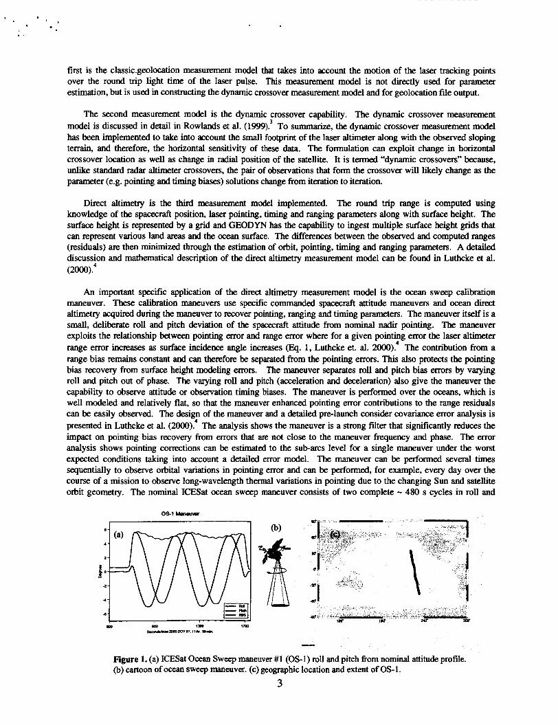
An important specific application of the direct altimetry measurement model is the ocean sweep calibration maneuver. These calibration maneuvers use specific commanded spacecraft attitude maneuvers and ocean direct altimetry acquired during the maneuver to recover pointing, ranging and timing parameters. The maneuver itself is a small, deliberate roll and pitch deviation of the spacecraft attitude from nominal nadir pointing. The maneuver exploits the relationship between pointing error and range error where for a given pointing error the laser althxter range error increases as surface incidence angle increases (Eq. 1, Luthcke et. al. The contribution from a range bias remains constant and can thedore be separated from the pointing errors. This also protects the pointing bias recovery from surface height modeling errors. The maneuver separates roll and pitch bias errors by varying roll and pitch out of phase. The varying roll and pitch (acceleration and deceleration) also give the maneuver the capability to observe attitude or observation timing biases. The maneuver is performed over the oceans, which is well modeled and relatively flat, so that the maneuver enhanced pointing error contributions to the range residuals can be easily observed. The design of the maneuver and a detailed pre-launch consider covariance error analysis is presented in Luthcke et al. ( ~ w o ) . ~ The analysis shows the maneuver is a strong filter that significantly reduces the impact on pointing bias recovery from errors that are not close to the maneuver frequency and phase. The error analysis shows pointing corrections can be estimated to the sub-arcs level for a single maneuver under the worst expected conditions taking into account a detailed error model. The maneuver can be performed several times sequentially to observe orbital variations in pointing error and can be performed, for example, every day over the course of a mission to observe long-wavelength thermal variations in pointing due to the changing Sun and satellite orbit geometry. The nominal ICESat ocean sweep maneuver consists of two complete - 480 s cycles in roll and

os1 Mawrrver

r - - I

--.

Figure 1. (a) ICESat Ocean Sweep maneuver #1 (OS-1) roll and pitch from nominal attitude profile. (b) cartoon of ocean sweep maneuver. (c) geographic location and extent of OS- 1.

3

0 .

. .

pitch where roll and pitch are offset in phase by onequarter of a cycle. Due to operational limitations an octagon, rather than a sinusoid, is used for both roll and pitch to approximate a cone “sweeped” out in space. For ICESat, the amplitude of the “cone” can be either 3 or 5 degrees, determined to be the optimal range in the analysis discussed in Luthcke et al. ( ~ o o o ) . ~ The total time for a single maneuver takes approximately twenty minutes. An ICESat Ocean sweep maneuver is shown in Figure 1.

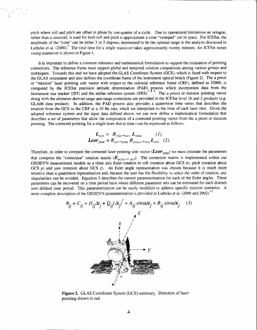
It is important to define a common reference and mathematical formulation to support the estimation of pointing corrections. The reference frame must support global and temporal solution comparisons among various groups and techniques. Towards this end we have adopted the GLAS Coordinate System (GCS), which is fixed with respect to the GLAS instrument and also defines the coordinate frame of the instrument optical bench (Figure 2). The a priori or “mission” laser pointing unit vector with respect to the celestial reference frame (CRF), defined as 52000, is computed by the ICESat precision attitude determination (PAD) process which incorporates data from the instrument star tracker (IST) and the stellar reference system (SRS). The a priori or mission pointing vector along with the altimeter derived range and range corrections are provided in the ICESat level l b and 2 products (e.g. GLA06 data product). In addition, the PAD process also provides a quaternion time series that describes the rotation from the GCS to the CRF at a 10 Hz rate, which we interpolate to the time of each laser shot. Given the adopted reference system and the input data defined above, we can now define a mathematical formulation that describes a set of parameters that allow the computation of a corrected pointing vector from the a priori or mission pointing. The corrected pointing for a single laser shot at time t can be expressed as follows.

7 8 9

Therefore, in order to compute the corrected laser pointing unit vector (fior,,) we must estimate the parameters that comprise the “correction” rotation mamx (RGCScor-) &. The correction matrix is implemented within our GEODYN measurement models as a three axis Euler rotation in roll (rotation about GCS x), pitch (rotation about GCS y) and yaw (rotation about GCS z). An Euler angle representation was chosen because it is much more intuitive than a quaternion representation and, because the user has the flexibility to select the order of rotation, any singularities can be avoided. Equation 3 describes the current parameterization for each of the Euler angles. These parameters can be recovered on a time period basis where different parameter sets can be estimated for each distinct user defied time period. This parameterization can be easily modified to address specific mission scenarios. A more complete description of the GEODYN parameterization is provided in Luthcke et al. (2000 and 2o02).4”

8..=C..+D..Af.+Q..(At.f+A..sin0At.+B..sinwAt (3) 9 9 9 1 9 1 9 I 9 j

Figure 2. GLAS Coordinate System (GCS) summary. Direction of laser pointing shown in red.

4

In practice, there are two references from which we compute the corrected laser pointing unit vector: (1) from the mission pointing as shown in the equations above (L,) and (2) with respect to the z axis of the GCS (substitute a O,O,l column vector for LGcs in Eq. 2. By design the GLAS laser pointing unit vector will be updated with new estimates of biases and corrections as the mission and calibration analysis progresses. For example, various releases of the GLA06 data product have different laser pointing biases applied as the knowledge of these biases has improved from our calibration analysis. Therefore, the recovered Euler angle correction matrix paramems will be different between these product releases. However, the G C S z axis provides a constant reference to compute the correction matrix. Therefore, we can compute our Euler angle correction parameters with respect to the mission pointing to understand the errors present in the current estimate of the laser pointing, and with respect to the GCS z axis to compare pointing in a common reference frame over the course of the mission.

EARLY MISSION POINTING, RANGING AND T ” G CALIBRATION

At the time of writing this paper, approximately 36 days of data have been collected from the operation of laser number one in the 8day repeat calibration orbit. Beginning on February 20,2003 laser #1 collected approximately 29 days of data while in sailboat attitude mode (GCS y axis along velocity vector), and another 7 days of data while in airplane attitude mode (GCS x axis along velocity vector). During this time period, data from six Pacific ocean sweeps were acquired with two ocean sweeps on each day of year (MY) 67,75 and 87. The details of each of the ocean sweeps that acquired data during this initial phase of the mission are given in Table 1. Our initial calibration efforts have focused on the analysis of the ocean sweep direct altimetry range data and dynamic crossovers from a nine-day time period encompassing the four sailboat mode ocean sweeps. The 9-day time period begins with track 59 of ICESat repeat cycle 3 and ends with track 74 of cycle 4 (approximately March 8’-17’ of 2003) we term this time period “cycle 3.5”. While future plans include the processing of crossovers from all available repeat cycles and direct altimetry to precisely mapped surfaces along with the ocean sweeps, the ocean sweeps and cycle 3.5 crossovers are the data selected for our initial calibration analysis presented here.

Table 1. Pacific ocean sweep details.

Ocean DOY Night/Day Maneuver Attitude Sweep 2003 Amplitude Mode os- 1 67 Night 5O Sailboat o s - 2 67 Day 5O Sailboat O S 3 75 Night 3 O Sailboat os-4 75 Day 3 O Sailboat OS-5 87 Night 5” Airplane OS-6 87 Night 5O Airplane

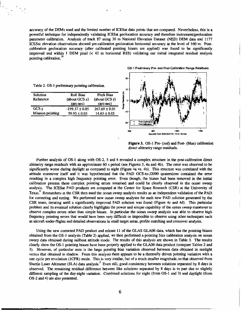
Our preliminary calibration efforts were focused on removing large-scale pointing biases to provide an initial significant improvement in geolocation. Towards this end, we analyzed the direct altimeter range data from ocean sweep 1 (OS-1) as soon as these data were made available. The recovered pointing biases are presented in Table 2 along with the solution formal errors. The results are shown relative to both the GCS z axis and the mission pointing provided on release 9 of the GLA06 data product. Figure 3 shows the pre- and post-calibration solution ocean sweep direct altimetry range residuals computed using a mean sea surface grid derived from over a decade of satellite radar altimetry.’ The pointing error is quite evident in the pre-calibration residuals (red data points) and a range residual reduction from 10.15 m RMS pre-calibration (red data) to 1.43 m Rh4S post-calibration (blue data) has been observed.

The pointing bias calibration has been independently validated using a profile matching technique where digital elevation models (DEMs) of sufficient accuracy and varying topography are compared with ICESat altimeter derived elevation The profiles are shifted in both the North-South and East-West directions until an optimal match is obtained. The magnitude of the shift represents a sample estimate of the geolocation accuracy in the horizontal direction. The accuracy of this validation technique is of course limited by the resolution and

5

accuracy of the DEMs used and the limited number of ICESat data points that are compared. Nevertheless, this is a powerful technique for independently validating ICESat geolocation accuracy and therefore instrumentlgeolocation parameter calibration. Analysis of track 87 using 30 m National Elevation Dataset (NED) DEM data and 1177 ICESat elevation observations showed precalibration geolocation horizontal accuracy at the level of 160 m. Post- calibration geolocation accuracy (after calibrated pointing biases are applied) was found to be significantly improved and within 1 DEM pixel (< 42 m horizontal RSS) validating our initial integrated residual analysis pointing calibration.'o

OS-1 Preliminary Pre- and Post-Calibration Range Residuals

Table 2. OS-1 preliminary pointing calibration.

Solution Roll Bias Pitch Bias Reference (about GCS x) (about GCS y)

(arc-Sec) (iUC-SeC)

GCS z -199.37 k 0.05 267.69 f 0.05 Mission pointing 59.93 k 0.05 14.65 f 0.05

P

10

-10

I I

Figure 3. OS-1 Pre- (red) and Post- (blue) calibration direct altimetry range residuals.

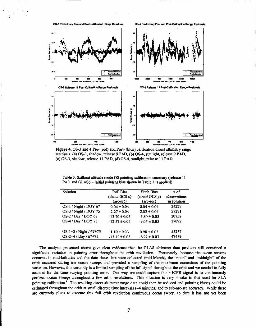
Further analysis of OS-1 along with OS-2, 3 and 4 revealed a complex structure in the postcalibration direct altimetry range residuals with an approximate 60 s period (see Figures 3,4a and 4b). The error was observed to be significantly worse during daylight as compared to night (Figure 4a vs. 4b). This structure was correlated with the attitude maneuver itself and it was hypothesized that the PAD GCS-to-J2000 quaternions contained the error resulting in a complex high frequency pointing error. Even though, the biases had been removed in the initial calibration process these complex pointing errors remained and could be clearly observed in the ocean sweep analysis. The ICESat PAD products are computed at the Center for Space Research (CSR) at the University of Texas.' Researchers at the CSR then used the ocean sweep analysis results as an independent validation of the PAD for correcting and tuning. We performed new ocean sweep analyses for each new PAD solution generated by the CSR team, iterating until a significantly improved PAD solution was found (Figure 4c and 4d). This particular problem and its eventual solution clearly highlights the power and unique capability of the ocean sweep maneuver to observe complex errors other than simple biases. In particular the ocean sweep analysis was able to observe high frequency pointing errors that would have been very difficult or impossible to observe using other techniques such as aircraft under-flights and detailed observations in small target areas, profile matching and crossover analysis.

Using the new corrected PAD product and release 11 of the GLAS GLA06 data, which has the pointing biases obtained from the OS-1 analysis (Table 2) applied, we then performed a pointing bias calibration analysis on ocean sweep data obtained during sailboat attitude mode. The results of this analysis are shown in Table 3. The results clearly show the OS-1 pointing biases have been properly applied to the GLAO6 data product (compare Tables 2 and 3). However, of particular note is the large pointing bias variation observed between data obtained in sunlight versus that obtained in shadow. From this analysis there appears to be a thermally driven pointing variation with a one cycle per revolution (ICPR) mode. This is very similar, but of a much smaller magnitude, to that observed from Shuttle Laser Altimeter (SLA) data analysis.2 Even still, good consistency between solutions separated by 8 days is observed. The remaining residual difference between like solutions separated by 8 days is in part due to slightly different sampling of the day-night variation. Combined solutions for night (from OS-1 and 3) and daylight (from OS-2 and 4) are also presented.

6

* . ‘ . ..

‘1 W

OS-3 Reham 11 PossCalbratpn Range Residuals OS4 R- 11 Post-Qllba(ion Rang@ RWidua$

- ‘ O l

‘1 10

-20 -I Figure 4.0s-3 and 4 Pre- (red) and Post- (blue) calibration direct altimetry range residuals. (a) OS-3, shadow, release 9 PAD, (b) OS-4, sunlight, release 9 PAD, (c) OS-3, shadow, release 11 PAD, (d) OS-4, sunlight, release 1 1 PAD.

Table 3. Sailboat attitude mode OS pointing calibration summary (release 11 PAD and GLA06 - initial pointing bias shown in Table 2 is applied).

Solution Roll Bias Pitch Bias # of (about GCS x) (about GCS y) observations

(arc-sec) (XC-SeC) in solution OS- 1 / Night / DOY 67 0.04 f 0.04 0.05 f 0.04 24227 OS-3 / Night / DOY 75 2.27 f 0.04 2.02 f 0.04 2927 1 OS-2 / Day / DOY 67 -13.70 f 0.05 -5.80 f 0.05 20758 O S 4 / Day / DOY 75 -12.57 f 0.04 -9.05 f 0.05 27092

OS-1+3 /Night / 67+75 1.10 f 0.03 0.98 f 0.03 53237 OS-2+4 / Day l67+75 -13.12 f 0.03 -6.92 f 0.03 47439

The analysis presented above gave clear evidence that the GLAS altimeter data products still contained a significant variation in pointing error throughout the orbit revolution. Fortunately, because the ocean sweeps occurred in mid-latitudes and the date these data were collected (mid-March), the “noon” and “midnight” of the orbit occurred during the ocean sweeps and provided a sampling of the maximum excursions of the pointing variation. However, this certainly is a limited sampling of the full signal throughout the orbit and we needed to fully account for the time varying pointing error. One way we could capture this -1CPR signal is to continuously perform ocean sweeps throughout a few orbit revolutions. This situation is very similar to that used for SLA pointing calibration.’ The resulting direct altimeter range data could then be reduced and pointing biases could be estimated throughout the orbit at small discrete time intervals (-4 minutes) and to sub-arc-sec accuracy. While there are currently plans to execute this full orbit revolution continuous ocean sweep, to date it has not yet been

7

* .

..

implemented. Therefore, in order to capture the orbital pointing error variation, we simultaneously processed the GLAS direct altimeter range data from the four sailboat mode ocean sweeps along with dynamic crossovers computed using 9days of data acquired during cycle 3.5. The crossovers are predominantly in the high-latitudes (-90% above 60" latitude), while the ocean sweeps provide a wealth of data in the mid-latitudes. Therefore, processed together these two data types compliment each other well and provide the ability to observe the pointing variation throughout the orbit revolution

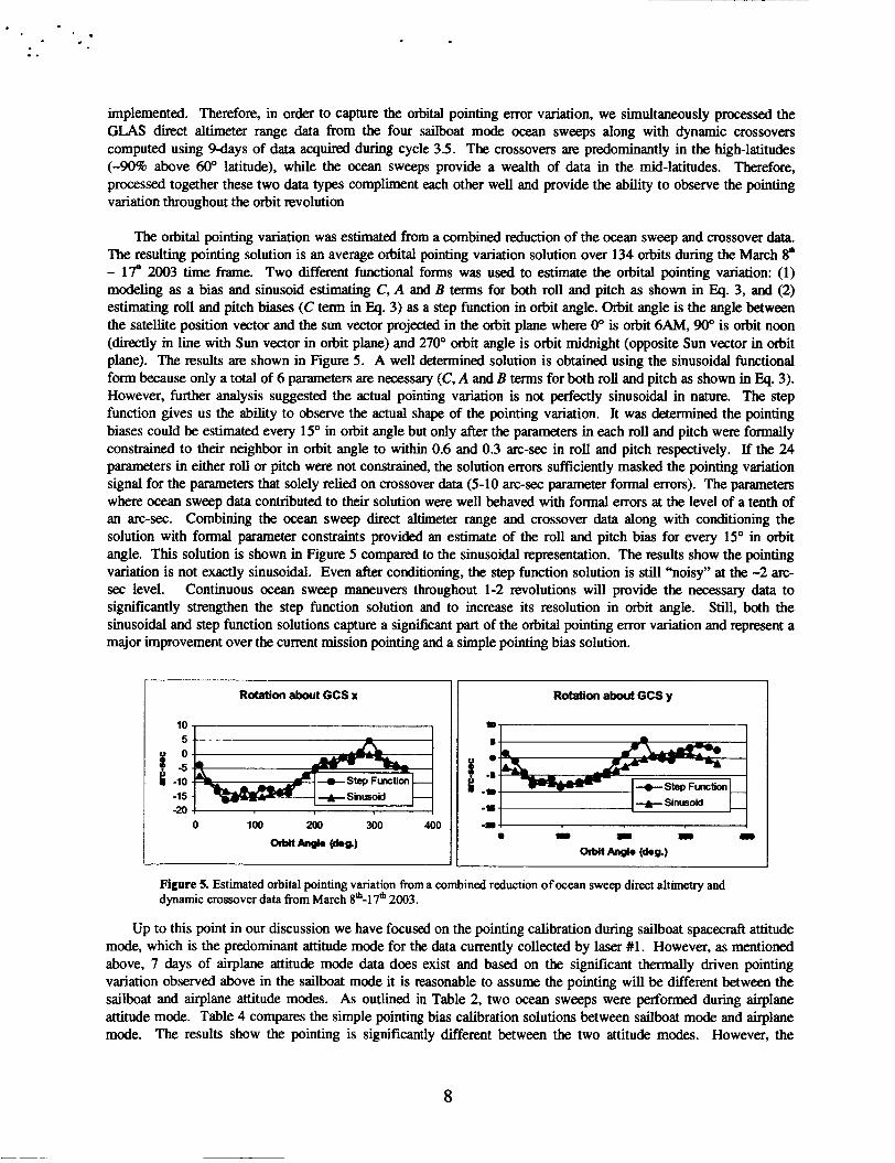
The orbital pointing variation was estimated from a combined reduction of the ocean sweep and crossover data. The resulting pointing solution is an average orbital pointing variation solution over 134 orbits during the March 8" - l? 2003 time frame. Two different functional forms was used to estimate the orbital pointing variation: (1) modeling as a bias and sinusoid estimating C, A and B terms for both roll and pitch as shown in Eq. 3, and (2) estimating roll and pitch biases (C term in Eq. 3) as a step function in orbit angle. Orbit angle is the angle between the satellite position vector and the sun vector projected in the orbit plane where 0" is orbit 6AM, 90" is orbit noon (directly in line with Sun vector in orbit plane) and 270" orbit angle is orbit midnight (opposite Sun vector in orbit plane). The results are shown in Figure 5. A well determined solution is obtained using the sinusoidal functional form because only a total of 6 parameters are necessary (C, A and B terms for both roll and pitch as shown in Eq. 3). However, further analysis suggested the actual pointing variation is not perfectly sinusoidal in nature. The step function gives us the ability to observe the actual shape of the pointing variation. It was determined the pointing biases could be estimated every 15" in orbit angle but only after the parameters in each roll and pitch were formally constrained to their neighbor in orbit angle to within 0.6 and 0.3 arc-sec in roll and pitch respectively. If the 24 parameters in either roll or pitch were not constrained, the solution errors sufficiently masked the pointing variation signal for the parameters that solely relied on crossover data (5-10 arc-sec parameter formal errors). The parameters where ocean sweep data contributed to their solution were well behaved with formal errors at the level of a tenth of an arc-sec. Combining the ocean sweep direct altimeter range and crossover data along with conditioning the solution with formal parameter constraints provided an estimate of the roll and pitch bias for every 15" in orbit angle. This solution is shown in Figure 5 compared to the sinusoidal representation. The results show the pointing variation is not exactly sinusoidal. Even after conditioning, the step function solution is still "noisy" at the -2 arc- sec level. Continuous ocean sweep maneuvers throughout 1-2 revolutions will provide the necessary data to significantly strengthen the step function solution and to increase its resolution in orbit angle. Still, both the sinusoidal and step function solutions capture a significant part of the orbital pointing error variation and represent a major improvement over the current mission pointing and a simple pointing bias solution.

Rotation about GCS x

-20 .I I

Rotation about GCS y

+Sinusoid --

Figure 5. Estimated orbital pointing variation from a combined reduction of Ocean sweep direct altimetry and dynamic crossover data from March 8*-17* 2003.

Up to this point in our discussion we have focused on the pointing calibration during sailboat spacecraft attitude mode, which is the predominant attitude mode for the data currently collected by laser #l. However, as mentioned above, 7 days of airplane attitude mode data does exist and based on the significant thermally driven pointing variation observed above in the sailboat mode it is reasonable to assume the pointing will be different between the sailboat and airplane attitude modes. As outlined in Table 2, two ocean sweeps were performed during airplane attitude mode. Table 4 compares the simple pointing bias calibration solutions between sailboat mode and airplane mode. The results show the pointing is significantly different between the two attitude modes. However, the

8

' . ..

magnitude of the pointing change observed between the two attitude modes is certainly consistent with the thermally induced orbital pointing variation observed during sailboat mode. These results emphasize a detailed pointing calibration will be necessary for each attitude mode and instrument laser change. Further analysis is necessary to fully calibrate laser pointing in the airplane attitude mode.

Table 4. Comparison of pointing calibration between sailboat and airplane attitude modes (release 11 PAD and GLA06 - initial pointing bias shown in Table 2 is applied)

Solution Roll Bias Pitch Bias # of (about GCS x) (about GCS y) observations

(iUC-SeC) (iUOSeC) in solution Sailboat mode OS-1+3 /Night 1.10 f0.03 0.98 f0.03 53237 DOY 67+75 Airplane mode OS-7+8 / Night -5.39 f 0.03 25.16 f 0.03 58383 DOY 87

Although our efforts have been concentrated on pointing calibration during this initial mission calibration effort, we have performed some limited analysis towards calibrating both range and timing. In order to calibrate range bias we performed a reduction of 1 s rate ocean direct altimeter range data from -9days during the cycle 3.5 time period. A summary of the range bias recovery is presented in Table 5 and indicates the altimeter is ranging long by 43.2 cm. Of course, this is a function of the altimeter tracking point offset used and the way in which the ranges are computed (waveform centroid) for this particular analysis. By design, pointing bias recovery from ocean sweep direct altimetry is insensitive to timing bias. However, pointing bias recovery from crossovers is sensitive to observation timing bias, and therefore, an observation timing bias must be simultaneously estimated when performing a calibration based on crossover data. Table 5 presents the recovered observation timing bias solution determined from the combined reduction of cycle 3.5 crossover and ocean sweep direct altimeter range data.

Table 5. Preliminary Range and Observation Timing Bias Solution

BiasType Dataused Estimate

43.2 k 0.1 cm Range 165357, l/s ocean direct

Observation Timing Bias altimeter range and 7441 6.5 f 0.3 ms

altimeter range observations 103 126 ocean sweep direct

dynamic crossover observations

CONCLUSIONS and FUTURE WORK

From the analysis presented in this paper it is evident that much progress has been made in calibrating the ICESat instrument/geolocation parameters of pointing, ranging and timing. While this analysis is preliminary and based on a limited amount of early mission data we have already significantly improved upon the initial calibration efforts. The ocean sweep technique was shown to be a powerful tool for the calibration of pointing biases at the sub-arc-sec level. In addition, the ocean sweep technique uniquely observed significant high-frequency errors in the early mission PAD solutions that have now been corrected. Analysis of direct altimetry from ocean sweep data taken in both sunlight and shadow has revealed a large (amplitude -17 arc-sec) thermally driven orbital variation in the pointing. Through the combined reduction of both ocean sweep direct altimeter range and dynamic crossover data we have been able to calibrate the orbital variation in pointing below the 2 arc-sec level. Even at this early stage of the mission and calibration efforts the analysis shows we are very close to the mission pointing requirement of 1.5 arc-sec. A preliminary solution for ranging and timing biases was performed using both direct altimeter range and

9

dynamic crossover data. ms. Additionally, initial in sailboat mode.

Range bias was found to be 43.2 cm while the observation timing bias was found to be 6.5 analysis of airplane mode data has revealed a significant pointing change from that found

While significant improvement in pointing, ranging and timing has been realized through this preliminary calibration effort, errors still remain and further improvement will be made. Future efforts will include the incorporation of SRS data into our orbital variation pointing calibration. In addition, a more detailed and complete analysis of airplane mode pointing, ranging and timing will be performed. An ocean sweep campaign is also planned. During this campaign at least two ocean sweep maneuvers will be performed on each day for an entire 8- day repeat. In addition, the ocean sweep maneuver will be continuously performed for at least one orbit revolution in the 8-day campaign period. These data along with dynamic crossover and SRS data will significantly improve our knowledge of the orbital pointing variation and biases. Additional improvements will be gained from a more detailed waveform analysis and resultant refmed range observation to be used in our calibration analysis. A more complete independent validation of our calibration and resultant improved geolocation will be performed using profile and waveform matching techniques. Even with these planned improvements, the prelimhary analysis presented in this paper has demonstrated the power of ocean sweeps and dynamic crossovers to calibrate pointing, ranging and timing in the presence of significant errors such as high-frequency PAD errors and large thermally driven orbital variations in pointing. The results emphasize the importance and demonstrate the capability of the integrated residual analysis calibration methodology to fully accommodate complex errors and not just simple biases.

The authors wish to thank the ICESat project for supporting this research effort. The authors also wish to thank the following individuals for the many fruitful technical discussions and various support: B. Schutz, C. Webb, S. Sirota, J. Abshire, S. Bae, L. Magruder and P. Millar. The authors also wish to thank members of the ICESat Science Computing Facility team for their continued efforts in providing and helping with the details of the ICESat data. In particular the authors wish to thank K. Barbieri, A. Brenner, J. Dimarzio and S. Bhardwaj.

REFERENCES

1 Zwally et. al., “ICESat’s laser measurements of polar ice, atmosphere, ocean and land,” Jouml of Geodymmics, Vol. 34, No. 34,2002, pp. 405-445.

2 Luthcke, S.B., C.C. Carabajal, D.D. Rowlands, “Enhanced geolocation of spaceborne laser altimeter surface returns: parameter calibration from the simultaneous reduction of altimeter range and navigation tracking data,” Journal of Geodynamics, Vol. 34, No. 34,2002, pp. 447-475.

3 Rowlands, D.D., D.E. Pavlis, F.G. Lemoine, G.A. Newumann, S.B. Luthcke, ‘The use of laser altimetry in the orbit and attitude determination of Mars Global Surveyor,” Geophysical Research Letters, Vol. 26, No. 9,1999, pp. 1191-1 194.

4 Luthcke, S.B., D.D. Rowlands, JJ . McCarthy, D.E. Pavlis, E. Stoneking, “Spaceborne laser-altimeter-pointing bias calibration from range residual analysis,” Journal of Spacecraft and Rockets, Vol. 37, No. 3,2000, pp. 374-384.

Rowlands, D.D., C.C. Carabajal, S.B. Luthcke, DJ. Hading, J.M. Sauber, J.L. Bufton, “Satellite laser altimetry: on-orbit calibration techniques for precise geolocation,” The Review of Laser Engineering, Vol. 28, No. 12,2000, pp. 7%-803.

5

GEODYN Operations Manual - 5 Volumes, NASNGSFC, Space Geodesy Branch, Code 926.

Bae, S.and B. Schutz, “Laser pointing determination using stellar reference system in Geoscience Laser Altimeter

6

7

System,” American Astronautical Society (00-123), 2000.

10

. . . c

b -

8 Bae, S. and B. Schutz, “GLAS Spacecraft Attitude Determination Using CCD Star Tracker and 3-axis Gyros,” American Astronautical Society (99-165),1999.

9 Sirota, M., P. Millar, E. Ketchurn, B. Schutz and S. Bae, “System to Attain Accurate Pointing Knowledge of The Geoscience Laser Altimeter,” American Astronautical Society (01-003), 2001.

Carabajal, C.C., D.J. Harding, J.L. Bufton, S.B. Luthcke and D.D. Rowlands, “ICESat Geolocation and Land Products Validation: Laser Altimetry Profile and Waveform Matching,” International Archives of Photogrammetry and Remote Sensing, ISPRS workshop proceedings, WG W3-WGIY2, Portland, OR, 17-19 June, 2003.

10

11