large-scale structure formation for power spectra with ... · large-scale structure formation for...

arX

iv:a

stro

-ph/

9507

036v

3 1

3 Ju

l 199

5Mon. Not. R. Astron. Soc. 000, 1–?? (1995) Printed 20 March 2018 (MN LATEX style file v1.4)

Large-scale structure formation

for power spectra with broken scale invariance

R. Kates, V. Muller, S. Gottlober, J.P. Mucket, J. RetzlaffAstrophysikalisches Institut Potsdam, Germany

Accepted Received ; in original form 1995

ABSTRACT

We have simulated the formation of large-scale structure arising from COBE-normalized spectra computed by convolving a primordial double-inflation perturbationspectrum with the CDM transfer function. Due to the broken scale invariance (’BSI’)characterizing the primordial perturbation spectrum, this model has less small-scalepower than the (COBE-normalized) standard CDM model. The particle-mesh code(with 5123 cells and 2563 particles) includes a model for thermodynamic evolution ofbaryons in addition to the usual gravitational dynamics of dark matter. It providesan estimate of the local gas temperature. In particular, our galaxy-finding procedureseeks peaks in the distribution of gas that has cooled. It exploits the fact that “cold”particles trace visible matter better than average and thus provides a natural biasingmechanism. The basic picture of large-scale structure formation in the BSI model isthe familiar hierarchical clustering scenario. We obtain particle in cell statistics, thegalaxy correlation function, the cluster abundance and the cluster-cluster correlationfunction and statistics for large and small scale velocity fields. We also report here ona semi-quantitative study of the distribution of gas in different temperature ranges.Based on confrontation with observations and comparison with standard CDM, weconclude that the BSI scenario could represent a promising modification of the CDMpicture capable of describing many details of large-scale structure formation.

Key words: primordial power spectrum – CDM – large-scale structure – galaxyclustering – cosmological velocity fields

1 INTRODUCTION

The search for a self-consistent model for the formation oflarge-scale structure capable of explaining the vast rangeof available observational data poses one of the greatestchallenges in theoretical astrophysics. In this paper, we willpresent strong evidence that a large body of observations isconsistent with a picture of structure formation based on a“double-inflationary” model (to be reviewed shortly). Themost directly relevant observations include the measuredlarge-scale anisotropy of the microwave background spec-trum (Smoot et al. 1992, Gorski et al. 1994), power spec-tra analysis of galaxy catalogs (Park et al. 1992, Vogeleyet al. 1992, Fisher et al. 1993), count-in-cell analysis of galax-ies (Efstathiou et al., 1990, Loveday et al. 1992), the galaxycorrelation function based on IRAS, CfA, and other cat-alogs (Loveday et al. 1992, Vogeley et al. 1992, Baugh &Efstathiou 1993), the angular correlation function of APMgalaxies (Maddox et al. 1990), abundance of clusters (Bah-call & Cen, 1993)) as a function of mass, rms line-of-sightpeculiar relative velocity of galaxy pairs (Davis & Peebles,

1983, Mo et al. 1993). Other observational quantities includelarge-scale velocity fields in general, the line-of-sight distri-bution of quasar absorption clouds, X-ray observations giv-ing information on the temperature and distribution of hotgas, the observed network of filaments and “walls”, the ex-istence of voids and their observed properties, and evidencefor the epoch of galaxy and cluster formation.

Prior to the analysis of the APM catalog and the COBEmeasurement of the large-scale microwave anisotropy, thebiased, σ8-normalized, flat CDM model (Blumenthal et al.1982) was quite successful in predicting the observed hier-archical network of filaments, pancakes and nodes and ob-served galaxy clustering (White et al. 1987). Biasing, orig-inally devised for explaining the enhanced correlation ofAbell clusters (Kaiser 1984), also had the advantage of re-ducing small-scale velocity dispersions to reasonable levels.These advantages disappear with the COBE normalizationof the CDM spectrum, because the antibiasing needed to ex-plain the observed variances of counts in cells is quite diffi-cult to reconcile with our observational knowledge of velocityfields and with other tests. More precisely: The normaliza-

c© 1995 RAS

http://arxiv.org/abs/astro-ph/9507036v3

2 R. Kates, V. Muller, S. Gottlober, J.P. Mucket, J. Retzlaff

tion fixed by the COBE anisotropy measurement appearsto imply excessive power in the small-scale (< 10h−1Mpc)regime of the primordial fluctuation spectrum P (k), whichmanifests itself in various conflicts with observations. Pre-dicted local velocity fluctuations seem to be quite in excessof measured relative pairwise line-of-sight projected veloc-ities (Davis & Peebles 1983), although the measurementsmay be sensitive to sampling effects (Mo et al. 1993).

COBE-normalized (flat) CDM simulations also predictmuch more pronounced and numerous bound structuressuch as massive galaxies and galaxy clusters than observed(Efstathiou et al. 1992). Relative to these massive structures,COBE-normalized CDM appears to imply fewer galaxies infilamentary structures than would be expected from obser-vations. In contrast, as we shall see, the double-inflationarymodels reproduce the observed filamentary structures rathereasily and predict fewer massive galaxies and clusters. Thedifferent evolution of filamentary structures may be intu-itively understood within the Zel’dovich (1970) picture ofanisotropic collapse of overdense regions leading to the for-mation of pancakes on a broad range of scales. In partic-ular, filaments are transitory structures: Due to the highnormalisation, the COBE-normalized CDM is further de-veloped, and therefore it is plausible that cooled materialin filaments will have more time to flow into large clumps(compare Doroshkevich et al. 1995).

On the other hand, “tilted” models (compare e.g. Cenet al. 1993) seem to have insufficient small-scale power: asa consequence, the predicted epoch of galaxy formation isdifficult to reconcile with the observation of high-redshiftobjects. Moderate-scale (60h−1Mpc) power may also be toolow, resulting in rather small streaming velocities. Mixeddark matter models (Davis et al. 1992, Klypin et al. 1993,Cen & Ostriker 1994) appear to agree better with a largebody of observations, but again the late epoch of galaxyformation may be problematic (Mo &Miralda-Escude, 1994,Kauffmann & Charlot, 1994).

Estimates of hot gas in clusters derived from X-rayobservations seem to imply that a high percentage of thedynamical mass may be in the form of baryons. E.g., forthe Coma cluster, White et al. (1994) compute that about30 % of the dynamical mass is in the form of hot gas. Ifthe estimate for Ωbh

2 ≈ 0.013 obtained from nucleosynthe-sis is applicable in clusters (unless significant segregationof hot gas in clusters has occurred), then the total mat-ter density in the universe would be restricted to the range0.1 < Ω < 0.3. Indeed, low-mass CDM models (Kofmanet al. 1993, Cen, Gnedin, & Ostriker 1993) with nonvanishingcosmological constant or low-mass and open CDM models(Kamionkowski et al. 1994) can explain the enhanced APMangular correlation function, probably the extended rangeof positive correlation of spatial galaxy correlation above30h−1Mpc, the cluster mass function, and the cluster-clustercorrelation function; however, the epoch of galaxy and clus-ter formation appears to be rather early. In particular, clus-ters in open models tend to be highly developed and tightlybound, exhibiting less substructure than observed (Kaiser1991, Evrard et al., 1993).

In addition to strictly observational constraints, thetheoretical appeal of a model and its consistency with ourknowledge of particle physics also play an important role inits acceptance. Standard CDMwas very appealing because it

involved only one true fit parameter (the amplitude of pri-mordial fluctuations) together with one phenomenologicalparameter (biasing). “Low-mass” models are theoreticallyless attractive because they require a nonvanishing cosmo-logical constant in order to achieve a flat universe, as pre-ferred in an inflationary scenario. Tilted models introduceone additional parameter; however, the simplest scenario as-suming an exponential inflaton potential is not theoreticallywell founded. Mixed dark matter models also involve onlyone additional parameter: (essentially) the neutrino mass(since their number density is fixed). The double-inflationarymodel requires two independent parameters. In Section 2,we review this model and describe fits to data in the lin-ear regime (Gottlober, Muller & Starobinsky 1991, GMS91;Gottlober, Mucket & Starobinsky, 1994, GMS94) and in thePress-Schechter theory (Muller 1994a) resulting in the par-ticular “BSI” (Broken Scale Invariance) spectrum studied inthis paper.

Encouraged by the success of the BSI model in the lin-ear regime, we now present the results of numerical n-bodysimulations in order to test observational results requiringaccurate predictions in the nonlinear regime. Now, one ofthe subtleties of the nonlinear regime is that our incom-plete understanding of physical processes at relevant lengthscales causes theoretical uncertainties that may be compara-ble to observational uncertainties (cp. for example, Ostriker1993). Complicated, nonlinear feedback mechanisms governthe dynamics at scales below our numerical resolution. Inparticular, an adequate theory of galaxy formation (and per-haps evolution) together with significantly improved com-putational resources would obviate the necessity for intro-ducing simple phenomenological concepts such as biasing.However, an accurate description of galaxy formation re-quires a robust treatment of gas dynamics over vast rangesof scales, densities, and other conditions; dynamic computa-tion of heating and cooling, including thermal instability andionization; star formation, supernovae; proper handling ofthe chemical evolution of a multi-component medium — toname a few considerations. Significant progress in applyinga hydrodynamic approach to cosmology has been achievedby Katz & Gunn (1991), Navarro & Benz (1991), Cen & Os-triker (1992), Katz, Hernquist & Weinberg (1992), and bySteinmetz & Muller (1995). In particular, a hydrodynami-cal description is essential for studying the formation andinternal dynamics of clusters (Evrard 1990). A compara-tive review containing additional references is now available(Kang et al. 1994). An alternative hydrodynamical approachemphasizing thermal instability and the importance of feed-back mechanisms such as supernovae has been studied byKlypin, Kates & Khokhlov (1992; KKK92). Hydrodynamicsimulations are clearly superior for obtaining reliable small-scale predictions from models of large-scale structure forma-tion. However, a lack of computer resources still precludestheir general use for high-resolution cosmological applica-tions.

The numerical particle-mesh code used here (Kateset al. 1991, KKK91; Klypin & Kates 1992, KK) includes amodel for thermodynamic evolution of baryons in additionto the usual gravitational dynamics of dark matter (see Sec-tion 3). The code provides an estimate of the (suitably aver-aged) local gas temperature without the enormous computa-tional cost of a full hydrodynamical description. A resolution

c© 1995 RAS, MNRAS 000, 1–??

Large-scale structure formation for power spectra with broken scale invariance 3

of 5123 cells (2563 particles) was achieved. High resolutionis crucial in the present study in order to include the effectsof both enhanced large-scale power and modest (comparedto CDM) small-scale power in the same simulation.

As discussed in Section 2, considerable preliminary test-ing using both linear analysis (compare GMS94) and moder-ate (2563 cells) resolution (compare Gottlober 1994, Muller1994b, Amendola et al. 1995) was first carried out to obtainoptimal estimates for the parameters kbr and ∆ (see Section2 ). These preliminary investigations also provided roughestimates of the sensitivity of our results to “fine-tuning”of parameters (see Conclusions), box size, etc. The powerspectrum used in the highest-resolution simulations and itsimplementation in the numerical simulations will be givenin Section 2.

Simulation of the coupling of thermodynamic evolutionto gravitational dynamics provides us with important indi-rect information concerning observable quantities; see Sec-tion 4. In Section 5, we present our results on the evolu-tion of the mass distribution and, in Section 6, its relation-ship to thermodynamic evolution. Of particular interest arethe particle in cell fluctuations, the evolution of clusteringwith redshift and its dependence on the spectrum, redshift-dependence of thermodynamics and percentage of cooledparticles, the relation between density peaks and hot andcold particles.

In Sections 7 and 8 we discuss the results of galaxy iden-tification and galaxy clustering: galaxy mass function versusPress-Schechter theory; dependence on spectrum and red-shift; galaxy correlation function versus correlation functionof density peaks; clustering and other properties of galaxyclusters. The characteristic features of large- and small-scalevelocity fields for BSI spectra are presented in Section 9. InSection 10, we draw our conclusions.

2 BSI POWER SPECTRUM

Standard inflation produces primordial adiabatic densityperturbations P (k) ∝ kn with a spectral index n = 1 plussmall logarithmic corrections which stem from the slowlychanging horizon length during inflation, i.e. they dependon the inflaton potential. We propose an early cosmologicalevolution which produces a power spectrum with a breakat a characteristic scale by introducing more than one effec-tive field responsible for inflation (Starobinsky, 1985). Weuse the combined action of renormalization corrections anda massive scalar field as the source of a non-flat primordialperturbation spectrum (GMS91). This model decouples theclustering properties at large and small scales. It requirestwo new parameters in addition to the amplitude: First, theratio of the masses ∆ ≃ m/(6.5M) appearing in the La-grangian

L =1

16πG(R −

R2

6M2) +

1

2(φαφ

α −m2φ2) ; (1)

this ratio essentially determines the ratio of power at small(galactic) scales to that at very large cosmic scales. Second,the epoch of the transition between inflationary phases isrelated to the initial energy density m2φ2

0 of the scalar field.This epoch determines a characteristic length scale lbr ≡2π/kbr where the shape of the spectrum changes.

Figure 1. BSI power spectrum (solid line) compared with stan-dard CDM (dashed line), a ΛCDM model (dotted line), and aMDM spectrum (dash-dotted line).

In GMS94, linear theory predictions of double-inflationary models were compared with observational con-straints. Assuming COBE normalization, the tests appliedwere as follows: “counts in cells” of the IRAS and APM sur-veys, the APM galaxy angular correlation function, bulk-flow peculiar velocities, the Mach number test, and quasarabundance. The BSI models were shown to be in good agree-ment with all of these tests for the parameter regime definedby 2 ≤ ∆ < 4 and 0.5h−1Mpc< k−1

br< 5h−1Mpc, the lat-

ter corresponding to length scales lbr ≈ (3 − 30)h−1Mpc.Although some freedom is permitted by these constraints inthe choice of kbr (or lbr), the best fit seems to be given byk−1

br= 1.5h−1Mpc, ∆ = 3. These values also led to reason-

able effective biasing parameters in preliminary test simula-tions. In all simulation results reported here, the terminol-ogy “BSI spectrum” refers to these values of the parametersunless otherwise stated.

After convolution with the standard CDM transferfunction of Bond & Efstathiou (1984), taking Ω = 1 andh = 0.5, the power spectrum is used to generate the initialcondition of the numerical simulations described in the nextsection. Fig. 1 plots the transformed BSI spectrum in com-parison with the power spectra of the standard CDM model,a ΛCDM (λ ≡ Λ/3H2 = 0.8, Ω = 0.2) and an MDM model(ΩCDM = 0.7, Ων = 0.2, Ωb = 0.1). The standard CDMspectrum has much more power at all the relevant scalesfor galaxy formation, while BSI mostly resembles MDM atlarge scales, but has more power on small scales, almost ashigh as the ΛCDM model. An analytical fit to the primordialpotential spectrum is given by

k3Φ(k) =

4.2× 10−6[log (ks/k)]0.6 + 4.7 × 10−6 (k ≤ ks)

9.4× 10−8 log (kf/k) (k > ks)(2)

with ks = (2π/24)hMpc−1, kf = e56hMpc−1. However, fora proper representation of the transition regime, the numer-ically tabulated spectrum is preferable.

In Fig. 2 we show the predicted multipole moments ofthe anisotropies of CMB fluctuations calculated followingGottlober & Mucket (1991) in comparison with new mea-surements on the angular scale 2 < l < 1200. Our spec-

c© 1995 RAS, MNRAS 000, 1–??


Figure 2. Comparison of the cosmic background fluctuation mul-tipoles of BSI (solid line) and standard CDM (dashed line) witha series of experiments.

tra are normalized with the 10-variance of the fluctua-tions σT = (30± 7.5) µK/2.735K from the COBE first-yeardata (Smoot et al. 1992). The triangle denotes the first-yearCOBE result Qrms-PS = (16.7 ± 4)µK (for the spectralindex n = 1) which is approximately equivalent to our nor-malization. The other experimental data (courtesy of B. Ra-tra, from Bond 1994) are from left to right COBE, FIRS,Tenerife, SP91, SK93, the lower end of the PYTHON error,ARGO, MAX1 and MAX2, full and source free MSAM2and MSAM3, and the upper limits of WD and OVRO (fordetails see Bond 1994). The reanalysis of the COBE second-year data by Gorski et al. (1994) implies an about 25 percent higher normalization of the spectra (Gottlober 1994).Consequences of such an increase will be discussed in theconclusions.

3 NUMERICAL REALIZATION

Initial fluctuations corresponding to BSI and standard CDMpower spectra were generated as realizations of a Gaussianrandom field. Positions and velocities were assigned accord-ing to the Zel’dovich approximation at redshift z = 25 (al-though for larger boxes the Zel’dovich approximation couldhave been continued until a later epoch). The Euler–Poissonsystem describing the evolution of self-gravitating, collision-less matter was then evolved from z = 25 to z = 0 using theparticle-mesh (PM) code described in KKK91 and KK.

To cover a large range of the spectra, we performeda series of simulations with different box sizes (see Table1). Asterisks denote high resolution simulations(5123 cellsand 2563 particles); the remainder of the simulations wereperformed using 2563 cells and 1283 particles. The twohigh-resolution BSI simulations were performed in boxes of200h−1Mpc and 25h−1Mpc. BSI-200* is intended for anal-ysis of the large-scale matter distribution, while BSI-25*should provide good working accuracy on galactic scales.In order to highlight differences between BSI and standardCDM, a series of simulations with half of this resolutionwere performed using the same random seed in boxes ofsize 25h−1Mpc, 75h−1Mpc, 200h−1Mpc, and 500h−1Mpc.

Figure 3. Range of spectra realized in the simulations BSI-25 –500 (horizontal lines indicate kmin to kmax); also shown is thelinear theory BSI spectrum (dash-dotted line) and a reconstruc-tion assembled from the BSI simulations at z = 0 (full line).

lgrid gives the size of the particles used in the cloud-in-cell

mass assignment scheme as well as the formal resolution ofthe grid on which the gravitational force is calculated. TheNyquist wavelength 2π/kmax, which depends on the number

of particles used in the simulation, is four times larger thanlgrid. It corresponds to an upper limit for the realization of

initial perturbations in k-space. MB+DM is the total mass ofa particle. Finally, we compare the grid variances of densitycontrast σδ and peculiar velocities σv of the initial realiza-tion of the Gaussian random field with the expectations ofthe linear power spectrum,

σ2δ =

1

2π2

kmax∫

kmin

dk k2P (k), σ2v =

H20

2π2

kmax∫

kmin

dk P (k), (3)

where the numbers are given at z = 0 transformed accordingto the linear theory growth law. They describe the qualityof the realizations of the power spectra in the different sim-ulation boxes.

On the scale of 8 h−1Mpc, one often refers to the mea-sured unit variance of galaxy counts in spheres as deter-mined from the CfA-catalog ((Davis & Peebles, 1983). Usingthe first integral of Eq. 3 with a top-hat window of radius8 h−1Mpc, we infer σδ = 0.46 for the BSI power spectrum.Therefore we predict a (linear) bias of galaxies with respectto dark matter of b ≈ 2.2. For the standard CDM modelwe have on the other hand σ2

δ = 1.12, i.e. there the galaxiesshould be slightly antibiased.

4 THERMODYNAMIC ESTIMATES OF GAS

TEMPERATURES

As described in KKK91 and KK, estimates of the averagevalues of the local dark matter density and velocity and ofthe local baryon temperature can be obtained from simula-tions of large-scale structure (without direct simulation ofhydrodynamics) by following the thermal history of the gaswhile imagining that, smeared out over a sufficiently coarse

c© 1995 RAS, MNRAS 000, 1–??


Table 1. Parameters of the simulations

Simulation lgrid MB+DM σδ σδ σv σv

[h−1Mpc] [M⊙] [km s−1] [km s−1]

BSI-200* 0.39 2.6× 1011 2.28 2.25 490 483BSI-25* 0.05 5.2× 1008 4.60 4.69 223 219BSI-500 1.95 3.3× 1013 0.94 0.93 512 508CDM-500 1.95 3.3× 1013 3.02 2.99 1049 1040BSI-200 0.78 2.1× 1012 1.62 1.60 516 479CDM-200 0.78 2.1× 1012 5.43 5.36 1103 1068BSI-75 0.29 1.1× 1011 2.59 2.54 441 376CDM-75 0.29 1.1× 1011 8.79 8.65 1064 979BSI-25 0.10 4.1× 1009 3.85 3.76 269 219CDM-25 0.10 4.1× 1009 13.1 12.8 857 735

scale, baryons are transported with the dark matter; i.e.,ρgas ≡ ρΩb, where Ωb = 0.1 is the background fraction ofbaryons. The practical advantage of this picture is that thethermal history of the gas reduces to integration of one ormore ordinary differential equations along known trajecto-ries (those of the dark matter).

This description is certainly unproblematic before theformation of the first shocks, when the medium is still coldand fluctuations are small (we put Tgas = 0 at zstart = 25).As perturbations grow, eventually the first objects start tocollapse, producing caustics in the dark matter and shocks inthe gas. As simple pancake models show (Shapiro & Struck-Marcell 1985), shocks occur close to caustics.

The label “shocked” may be assigned to a particle in oneof two ways: First, particles for which the Jacobian deter-minant of the transformation from Lagrangian to Euleriancoordinates is negative are classified as shocked. (Particlelabels (i, j, k) are the numerical realization of Lagrangiancoordinates. The position assigned to a particle is the nu-merical representation of its Eulerian coordinates.) The Ja-cobian is determined for each particle by considering thevolume element constructed from the position vectors to itsnearest Lagrangian neighbors. Second, a particle inherits thelabel “shocked” by passing through a shocked region. Moreprecisely, if particle (i, j, k) is in cell (I, J,K), then the la-bel shocked is assigned to particle (i, j, k) if the density ofpreviously shocked gas is nonzero in cell (I, J,K) and allneighboring cells.

At a shock, the temperature acquired by gas particleswith velocity ~v is given by

kT ≈ µMmH(~v − ~U)2/3, (4)

where ~U is the local velocity determined by interpolation ofthe velocity field onto a coarse grid of twice the usual cellsize. (If it should happen that too few particles are presentto determine ~U , the temperature assignment is simply post-poned.) This estimate is relatively insensitive to small er-rors in the position of the shock. Here, mH is the massof hydrogen, and µM is the molecular weight per particle,µM ≈ (nH + 4nHe)/(2nH + 3nHe) ≈ 0.6.

When a particle crosses a shock and is assigned a tem-perature, we start to integrate the energy equation along thetrajectory of the particle:

dT

dt= (γ − 1)

(

T

nH

dnH

dt−

µM

µH

1

knH

(Λrad + ΛComp)

)

, (5)

where µH is the molecular weight per hydrogen atom, µH ≈(nH + 4nHe)/(nH ) ≈ 1.4, ρgas ≡ ρΩb = nHµHmH , andγ = 5/3. Here, Λrad represents radiative losses in the hotplasma with assumed primordial abundances, and ΛCompis the cooling rate due to Compton scattering. To estimateΛrad, we used analytic fits as in KK and KKK91 to thecooling curves given in Fall & Rees (1985). The medium istreated as optically thin and in collisional equilibrium.

Computation of the increment in T due to the (La-grangian) time derivative of nH in Eq. 5 requires a knowl-edge of nH at the present and at the previous timestep. Foreach timestep, we construct the “gas density” on the grid,defined by counting only contributions of shocked (hot) par-ticles. (For the dark matter density, one of course counts allparticles). For the evolution of Eq. 5, the present value ofnH for Eq. 5 is computed simply by interpolation to the po-sition of the particle and then stored for use at the followingtimestep.

Now, when material cools below 104 K, stars will form,producing luminous matter. By assigning the label “cooled”to the particles with T < 104 K, we have a measure for theamount of visible matter. However, we know that the effi-ciency for the conversion of gas to stars is low. One nonlin-ear feedback mechanism limiting star formation could be theenergy provided to the medium by supernova explosions. Asecond (also nonlinear) mechanism inhibiting star formationis ionization and heating due to ambient ultraviolet radia-tion. As emphasized by Efstathiou (1992), a similar mecha-nism could be responsible for suppressing the formation ofdwarf galaxies. It should be emphasized that some mecha-nism preventing conversion of the gas to luminous matter isnecessary in BSI models as well as in CDM and in the pre-COBE version of CDM: otherwise, all the gas would simplycollapse, forming stars and ending up in globular clusterslong before the formation of large objects.

In the present realization of the code, we take theseeffects into account in a crude and purely local manner:we “reheat” those particles to the temperature Treheat =5× 104 K which have cooled to below 104 K with a proba-bility Preheat and assign to the remaining particles the la-bel “cooled.” Some of the reheated particles later will attainhigh temperatures, provided they enter collapsing regions ofhigh density. Reheated particles can simply cool again andturn into “visible” matter. However, once cooled, a particlecannot be reshocked. The value Preheat was held constantat 85 per cent, the value estimated in KK for a 50 h−1Mpc

c© 1995 RAS, MNRAS 000, 1–??


grid and a σ8 normalized CDM spectrum to give a reason-able fraction of hot gas in clumps of galactic mass (about10 per cent). The fraction of cooled gas (88 per cent) for acell size of about 0.05h−1Mpc in the highest resolution BSIsimulation seems to be reasonable. The distribution of par-ticles of different temperature ranges, variation with cell sizeand spectrum, and related considerations will be discussedbelow in Section 6.

We recall that the mean density of stars (and othercomponents of the baryonic matter) in some comoving celldepends in principle on the entire past history of the cell andnot just on its density at some particular epoch. As discussedin KKK91 and KK, comparison of the density distributionof “cold” material – which is related to the density of visiblematter – with the dark-matter density thus yields informa-tion useful for testing cooling as a physical mechanism for“biased galaxy formation.”

A reasonable upper bound for the aforementioned“coarse graining” (i.e., error in predicting positions ofbaryons) is the local sound velocity integrated over a Hubbletime (e.g., for T ≈ 5×106 K it is 2 or 3h−1Mpc). However, intests – leaving aside conditions prevailing in clusters – for abox of 75 h−1Mpc (cell length 200 h−1kpc), the error seemsto be of the order of the cell resolution only. The explanationseems to be that both components move in the same poten-tial well. The dark matter spends a large fraction of its timeat about the same radius as the gas, because they originallyhad the same kinetic energy. Due to mixing, the dynam-ics of dark matter particles bears some resemblance to thedynamics of a gas whose temperature corresponds to the lo-cal velocity dispersion. Incidentally, from experiments withtruncated spectra in KKK91 and from theoretical consider-ations, we know that temperature predictions are somewhatsensitive to the portion of the spectrum actually simulated.This fact implies that the same spectrum simulated in boxesof varying sizes can yield varying estimates of temperaturedistributions.

Results of a 1D-pancake test presented in KKK91 showgood agreement of our model with hydrodynamical simula-tions (20 per cent of gas cooled, position of cooling front andshock wave). Proper inclusion of hydrodynamics and the ef-fects of thermal instability would be expected to make a sig-nificant difference in at least two situations: First, when gasstarts to cool efficiently – this happens inside dense regionsand/or if the temperature becomes too low (T < 2×105 K).Second, when gas undergoes secondary shocking – for ex-ample, in collapse to objects with masses smaller than agalactic mass (for more detailed comparison, see, KKK92).Thus, the code does not properly treat the internal regionsof galaxies and clusters, but it would be expected to give areasonable approximation for the temperature and distribu-tion of gas which leaves voids and is trapped in the potentialwells of superclusters and filaments. Comparison with Cen &Ostriker (1992) supports this expectation: the baryonic anddark matter distributions look remarkably similar; most ofthe gas in regions with density ρ > 10〈ρ〉 has a tempera-ture between 106 K and 107 K, similarly to what was foundin KK. Comparison with hydrodynamic simulations of peri-odic disturbances reported in KKK92 also lead to reasonablequalitative agreement in this regime.

Figure 4. Comparison of the variances of counts in cells of galax-ies of the Stromlo–APM (full circles) and IRAS (triangles) surveywith the variances of the dark matter particles in the simulations.The BSI curve (solid line) composed from the simulations withdifferent box sizes fits the data quite well. The dashed line corre-sponds to the CDM simulations. Dashed-dotted and dotted linesare the linear theory predictions of BSI and CDM, respectively.

5 COUNT-IN-CELL ANALYSIS FOR DARK

MATTER

One useful method of characterizing the dynamics of clus-tering is to study the statistics of counts in cells. It is arobust measure for distinguishing different power spectra.For example, the rms fluctuations of simulated dark matterparticles in a sphere of radius 8h−1Mpc are often used todetermine the linear biasing factor. The fluctuations on thescale of a galactic halo provide an estimate of the thresholddensity contrast required in galaxy identification algorithms.Comparison of the simulated count fluctuations as a functionof radius with rms fluctuations observed in the IRAS cata-log (Efstathiou et al. 1990a) and the Stromlo-APM survey(Loveday et al. 1992) provides an important test of models.

In Fig. 4 the curves representing COBE-normalized BSIhave been shifted vertically by a “biasing” factor bBSI = 2 inorder to normalize fluctuations to observations at 8h−1Mpc,while the CDM curves had bCDM = 0.9. CDM fluctua-tions are too low (significantly outside the 1-σ error rangeon the low side) on scales (15− 50)h−1Mpc, after which themeasurement errors increase. In contrast, the interpolationcurves in the range of BSI simulations fit the data quitewell. The good fit beyond about 15h−1Mpc is consistentwith the predictions of linear analysis (GMS94). The slightdifferences at small scales are due to the difference betweenlinear and nonlinear evolution. The variances of cell countsare calculated in real space. At the scales studied the lineartheory predicts a constant amplification factor which can beincorporated in the value of the bias parameter. The mea-sured variances provide a good test of the slope of the BSIpower spectrum. In contrast, the CDM counts in cells areinconsistent with observations at about the 2-σ level.

The redshift dependence of the probability distributionof particle-in-cell counts delivers an estimate of the non-linearity of clustering. Using the counts on a 1283 grid ofthe 200 h−1Mpc-simulations, we compare BSI and CDMsimulations in Fig. 5. Over four decades in the probability

c© 1995 RAS, MNRAS 000, 1–??


Figure 5. Particle-in-cell distribution of BSI-200 (full lines)and CDM-200 (dashed lines) simulations. The curves (z =2, 1.5, 1, 0.5, 0) show the dependence of the probability distribu-tion of grid cells on the number of particles in the cell; the curvesare steeper at higher redshift. For reference, a curve of slope −3 isdrawn, corresponding to an evolved stage of pancake formation.

it is remarkably well described by a power law φ(n) ∝ n−3,which is a prediction of the pancake model (Kofman et al.1993). The CDM models at z = 0 are less steep, correspond-ing to more big clumps in the matter distribution. The CDMmodels at about z = 2 had a similar slope to the BSI modelat z = 0. The subsequent evolution to a less rapid fall off is aquantitative measure of the substantially increased cluster-ing of CDM compared to BSI models. The large dynamicalrange of the dark-matter probability distribution as com-puted using the simulation cells is more of theoretical inter-est, and it cannot be compared directly with the one-pointdistribution function estimated from galaxy surveys.

6 GAS TEMPERATURES: STATISTICS AND

SPATIAL STRUCTURE

As explained in Section 4, the “temperature” assigned toeach particle depends on its complete history, including theepoch and conditions under which it was shocked and theenvironment (in particular the local density) at all interme-diate times since shocking. At a particular time, say z = 0,the gas temperature distribution thus contains more infor-mation than the density and velocity distributions alone.

In interpreting the numerically computed gas tempera-ture distribution, one should keep in mind the idealizationsand limitations involved. As discussed above, a proper hy-drodynamic treatment of the gas would be expected to makea systematic difference in regions with secondary shockingand/or very high density, in particular inside clusters andgalaxies. However, any treatment of the gas, even includinghydrodynamics, will contain numerical inaccuracies (result-ing both from limited resolution and from systematic errors)as well as theoretical uncertainties due to incomplete mod-elling. Bearing all of these errors and uncertainties in mind,we take a brief look at what can be learned from particletemperature statistics.

In Fig. 6, the percentage of particles in selected temper-ature ranges at z = 0 for BSI and CDM simulations is plot-

Figure 6. Percentage of particles in different temperature rangesas a function of cell size at redshift z = 0. Plus signs indicateCDM simulations, asterisks BSI, and diamonds high-resolution(5123 cells) BSI simulations. a) never shocked, b) cooled, c)temperature range 104 < T < 5 × 104, d) temperature range105 < T < 1.5× 106, e) temperature range T > 107.

ted against cell size, which for all simulations shown is in-versely proportional to the highest resolved wavenumber. In-deed, studies of truncated spectra in high-resolution simula-tions (KKK91) indicate that the wavenumber limit is crucialto temperature statistics, i.e., qualitatively similar trendswould be observed even if the spatial resolution were to beimproved while keeping the wavenumber limit constant. (In-cidentally, percentages do not add up to one, because thetemperature ranges shown are not exhaustive.) Plus signsindicate CDM simulations, asterisks and diamonds BSI; di-amonds indicate the high-resolution simulations, in whichthe ratio of highest to lowest resolved wavenumber is twice

c© 1995 RAS, MNRAS 000, 1–??


(a) (b)

Figure 7. Comparison of slices through 200h−1Mpc BSI (a) andCDM (b) simulations in the temperature range 104 K < T <

5× 104 K.

as large. One expects the (limited) spectral range to havean influence on gas temperature statistics, and this expec-tation is borne out in Fig. 6. The trend with respect to cellsize is different in different temperature ranges. However, themost striking regularity is that in all temperature regimes,a smooth (in most cases monotonic) trend is apparent uponplotting percentage against cell size (equivalently here: high-est resolved wavenumber) rather than box size (equivalentlyhere: lowest resolved wavenumber). A plot with respect tobox size would be obtained by shifting the high-resolutionpoints (diamonds) by one point to the right, which in allcases would move them off an otherwise smooth curve.

Fig. 7 illustrates a typical slice in the range 104 K< T < 5× 104 K for both BSI and CDM simulations. (Notethat the random seed used in BSI and CDM simulations wasthe same, resulting in the same phase relations for each per-turbation mode.) Slices are about 12h−1Mpc thick. About9000 particles are plotted in each slice (all of the particlesin the CDM slice and about 40 per cent of the particles inthe BSI slice). In Fig. 8, spatial distributions for BSI simu-lations are illustrated in the same thin slice for particles inthe ranges 105 K < T < 1.5 × 106 K, T > 107 K, cooled(T < 104 K), and never shocked. The different temperatureranges highlight quite different features of the distributionin a way that would not be possible using simple peak statis-tics.We now consider various temperature ranges in detail:Never shocked: This percentage is a measure of the frac-tion of particles not in pancakes. The fraction increasesmonotonically with cell size for both BSI and CDM (Fig.6a). The trend may be attributable to the fact that for largercell size, the portion of the spectrum actually simulated isshifted toward smaller wavenumbers, with correspondinglysmaller values of k3P (k), resulting in longer timescales forformation of structures such as pancakes. The number of un-shocked particles is consistently lower by a factor of aboutthree for CDM than for BSI, directly reflecting the signif-icantly enhanced small and medium-scale power of CDMcompared to BSI. In Fig. 8a, the spatial distribution of un-shocked particles is shown for a 25h−1Mpc high-resolutionsimulation. The distribution shows practically no structure,aside from being absent in regions of high density, whereall of the particles are shocked. Visual inspection of slicesconfirms one’s expectation that material in voids consistsmainly of unshocked particles.

Cooled: From plausibility arguments one expects the distri-bution of “cooled” particles to trace the galaxy (halo) distri-bution more accurately than does the unbiased dark-matterdistribution. (A higher probability of cold gas obviously fa-vors star formation.) The results of KKK91 in the contextof high-resolution, 2D simulations lend additional supportto this expectation: There, halos were found with high con-fidence by a (“friends-to-friends”) clustering algorithm ap-plied to all particles. The percentage of cold particles insidehalos was significantly higher than outside. Moreover, theepoch of galaxy formation (estimated by cluster analysis atvarious redshifts) agreed with the average redshift zgal at

which the cold particles in galaxies “cooled.” In three dimen-sions, we exploit the affinity of cooled particles for galaxiesin our galaxy-finding routines: As discussed in Section 7, theroutines begin by searching for peaks in the cooled-particledistribution.

As seen in Fig. 6b, the percentage of cooled particlesat z = 0 varies strongly with cell length (more precisely,with Nyquist frequency), mainly because power at smallerlength scales leads to early formation of small pancakes and,in spite of “reheating,” subsequent cooling. (The redshiftat cooling is recorded for each cooled particle.) Consider astructure of characteristic size L. Smaller structures are as-sociated on the average with smaller characteristic initialtemperatures (∝ L2, since typical relative velocities in Eq. 4scale with H0L). The CDM simulations have more small-scale power and therefore consistently fewer unshocked par-ticles and more cooled particles. In KKK91, it was shownthat truncation of the spectrum below the Nyquist frequencyleads to significant reduction of the number of cooled par-ticles (keeping spatial resolution constant). Thus, as in thecase of unshocked particles, the variations with “cell size”seen here can probably be attributed to changes in the rangeof the spectrum actually simulated. Filaments and voids areevident in the cold particle distribution; the hierarchy of fil-ament separations and void sizes give the visual impressionof a broad distribution of characteristic length scales.

Particles in the temperature range (1 − 5) × 104 K:

This temperature range would tend to be associated withLyman-α clouds. However, a more realistic treatment of theeffect of the ultraviolet background on the matter (includingionization and heating) would be required to draw quantita-tive conclusions concerning Lyman-α clouds. Such a treat-ment is discussed by (Mucket et al. 1995). Nevertheless, wemay obtain some hints as to what to expect from a morerealistic treatment by examining the trend in Figs. 6c. Thefraction grows monotonically both in BSI and in CDM withcell scale, except for the 500h−1MpcBSI simulation, withCDM consistently lower. A reasonable interpretation maybe that earlier pancake formation and efficient cooling atmoderate redshifts in the present code deplete the reservoirof particles (especially those near galaxies) that would other-wise be candidates for this temperature range. The turnoverof the BSI curve at large scales is not surprising, since atthe largest scales, the reservoir of shocked particles sets thelimit. (In any case, quantitative studies of Lyman-α cloudswould require resolution of about 50− 100 kpc.)

With proper treatment of ionization and heating, therelative fraction of cold particles would be expected to dropsignificantly in favor of particles in the range of tempera-tures (1 − 5) × 104 K, except in very dense regions. Upon

c© 1995 RAS, MNRAS 000, 1–??


examination of numerous slices, there is the visual impres-sion that particles in the temperature range (1− 5)× 104 Kat least roughly trace the distribution of cold particles atz = 0. This may be a hint that a population of Lyman-αclouds could be associated with galaxies (cp. Petitjean et al.1995).

Comparing BSI and CDM slices for the temperaturerange considered in Fig. 7, there is a strong impression ofthinner, better defined filaments and emptier voids in CDMthan in BSI simulations. (Note that the total number ofparticles is the same.) This impression is consistent withthe interpretation that the standard CDM looks like theBSI model would look like if it were evolved to a largerfluctuation amplitude.Particles in the temperature range 105 K < T <1.5×106 K: As explained in KK, there are strong theoreticaland observational reasons for an association between gas inthis “warm” temperature range and filamentary structures.In Fig. 8c, it is evident that warm particles trace filamentsquite closely in BSI. The same qualitative picture is foundin all boxes. Comparison of CDM and BSI simulations inthis warm regime shows little qualitative difference in fila-mentary structures, except that CDM consistently leads tosomewhat more gas in the warm regime than BSI. This oc-curs despite CDM’s enhanced accumulation of material inclusters, which would tend to transfer gas from the warm tothe hot regime (see discussion of hot gas below). The trendtoward more warm gas at larger simulations may be relatedboth to the increased reservoir of shocked, but not yet cooledparticles (an essentially small-scale effect) and perhaps theinfluence of large-scale power in the portion of the spectrumactually simulated. This second cause is consistent with arise just visible in the BSI curve at cell-size 0.39h−1Mpc(high-resolution simulation).Particles in the temperature range T > 107 K: The“hot” gas represented by these particles is generally associ-ated with the deep potential wells of clusters, and thereforeit is no surprise that in Fig. 8d hot gas traces clusters (alsoverified by comparison with galaxy catalogs). The percent-age of “hot” particles with T > 107 K, which are nearlyall associated with clusters or large galaxy groups, is consis-tently an order of magnitude higher for CDM than for BSI,the trend becoming even stronger at larger cell size. Thistrend is consistent with the general conclusion that CDMcauses more and larger massive structures (also evident inslices). Moreover, these structures seem to be farther evolvedin CDM, so that deep potential wells would also tend to bebroader. Broader cluster potential wells would explain whythe disparity between CDM and BSI grows at larger celllengths (Fig. 6e). Cluster potential wells are still fairly wellresolved at the poorest resolution in CDM, but not in BSI.

7 GALAXY IDENTIFICATION AND

STATISTICS

The galaxy finding procedure used here was a modified den-sity peak prescription: Based on the results of KKK91, KK,cooled particles are preferred tracers of the galaxy distribu-tion. We therefore began by searching for local maxima ofthe density field of cold particles exceeding a predeterminedthreshold value δth. (The local maxima were also required

(a) (b)

(c) (d)

Figure 8. Slices of BSI-25* simulation at z=0. a) unshocked; b)cooled; c) 105 K < T < 1.5× 106 K; d) T > 107 K.

to be maxima within a 53 cell neighborhood.) The mass ofthe corresponding galaxy was then computed by summingthe contributions of all particles within 0.5 cell lengths ofthe maximum in the lower resolution simulations and withinone cell lengths of the maximum in the high resolution sim-ulations. This leads to the same physical length for selectinghalos in simulations of the same box size, i.e. to comparablecatalogues. Since the centroid can shift due to addition ofnew particles, the procedure was iterated six times, and acentroid, velocity, and mass were assigned to the galaxy. Foreach simulation, several galaxy catalogs were constructed us-ing various choices of threshold. Appropriate choices lie inthe range δth = (1.5−3)σδ . In the end, one seeks a catalog in-cluding at least as many galaxies as would be expected fromobservational counts of galaxies with luminosities exceed-ing the characteristic Schechter luminosity L∗ in the givenvolume. For numerical simulations, the mass correspondingto “L∗”-galaxies can only be determined from this require-ment a posteriori. We observed that reducing the thresholdsimply resulted in including additional galaxies at the lowend of the mass spectrum, but had virtually no effect onthe galaxies at higher masses. Thus we can extract one biggalaxy catalog from each simulation, which can be cut off atthe low-mass end as required. A natural cut-off is impliedby the finite resolution of the simulations. At later stages,this cut-off grows due to the overmerging effect.

In Fig. 9 we compare mass functions derived from thesmall box simulations where we expect the most reliableidentification of single galactic halos. The halo masses spanthe range from 1010M⊙ to 4 × 1012M⊙, and they can befitted by Schechter curves of the form

dn/d logM = n∗(M/M∗)−p exp(−M/M∗), (6)

For BSI-25* we get M∗ = 1012M⊙, n∗ = 2.6×10−2h3Mpc−3

c© 1995 RAS, MNRAS 000, 1–??


Figure 9. The ’galaxy’ mass function of BSI-25 (thin solid his-togram), of BSI-25* (thick solid histogram) compared with theCDM-25 function (dashed histogram). The solid and dash-dottedcurves correspond to comparison Schechter curves with parame-ters provided in the text.

Figure 10. The halo mass function of BSI-25 at redshifts z =2, 1.5, 1, 0.5, 0. For z = 0 a best fit Schechter distribution is shownusing a characteristic mass M∗ = 6 × 1011M⊙, a power indexp = −1.1 and mass density n∗ = 1.4× 10−2h3Mpc−3.

and p = 0.8, compare the solid line in Fig. 9. The lowerdashed line represents the observational results from Efs-tathiou et al. (1988), n∗ = 1.6 × 10−2h3Mpc−3, p = 0.1,and also M∗ = 1012M⊙ (assuming a quite high M/L ratioof about 100M⊙/L⊙). Similar parameters of the Schechterfunction are derived in Loveday et al. (1992).

The simulated mass spectra lead to approximately thesame abundance of M∗ galaxies as the observations. Com-parison of galaxy mass spectra between CDM and BSI sim-ulations at the same resolution shows that the CDM leadsto a slower inclination at small masses, despite of the ex-cessive power at small scales. Due to overmerging (Katz &White 1993; Kauffmann et al. 1993), however, we know thatspectra from PM simulations may not be directly comparedwith observational data. One way to imagine how overmerg-ing comes about is as follows: Potential wells associated withgalaxies can generally bind particles with velocities of about250 km s−1. However, the potential wells in clusters can bind

Figure 11. The cumulative halo mass function of BSI-200* atredshifts z = 1.8, 0.67, 0.43, 0.25, 0.1, 0. The mass range corre-sponds to small groups of galaxies which undergo substantialgrowth after z = 1.8.

particles with velocities of about 1000 km s−1. The proba-bility that a particle within a cluster will be near one of thedeeper troughs may be slightly elevated, but not enough todistinguish galaxies, at least not using the present scheme atthe presently attainable resolution. In a hydrodynamic sim-ulation with proper treatment of cooling (Katz & Weinberg,1992, Katz & White, 1993, and Evrard, Summers & Davis1994), one would expect baryons to condense earlier in thegalaxy (halo) potential wells, before the galaxies are assem-bled in the cluster. On the other hand, the PM dynamicsleads to an merging of halos per se. We do not intend tomake predictions on the galaxy mass functions in BSI fromour simulations. We only use the halo identification schemeto get a catalog of objects with a reasonable number density,whose clustering properties should be characteristic for theprimordial perturbation spectrum.

In order to understand the development of (over-) merg-ing in a qualitative way, we studied the evolution of the massspectra of halos (massive galaxies and groups). The redshiftdependence of the differential galaxy mass function of BSI-25 is shown in Fig. 10. A Schechter fit is possible for allredshifts, only at z = 0 the number of very massive halosbegins to exceed the exponential fall-off. Note that whilethe number of low-mass halos (M < 1011M⊙) grows by lessthan a factor of two between z = 1 and z = 0, the number ofgalaxies of M > 5×1011M⊙ grows by a factor of about 10 ormore. The redshift dependence of cumulative mass functionsfor BSI-200* is shown in Fig. 11. Focusing our attention onthe behavior of the curves beyond 2 × 1013M⊙, we foundan increasing of the number of high-mass halos after aboutz = 0.67, suggesting that at earlier epochs (before clusterformation), overmerging may be less severe.

Summarizing, CDM appears to lead to more massiveobjects than BSI (compare in Fig. 9 the thin solid anddashed lines for BSI and CDM distributions, respectively).However, in view of overmerging, the apparent disagreementof mass spectra derived in both scenarios with mass spectrainferred from luminosity functions cannot be interpreted asa weakness of either model at the present stage.

We can gain important information from the spatial

c© 1995 RAS, MNRAS 000, 1–??


Figure 12. The correlation function of galactic halos (identifiedin BSI-200*, (dash-dotted line) and of cluster halos (using BSI-500, solid line). For comparison we show a straight line with slope1.6

distribution and velocities of galaxies that are derived fromour catalogs.

In Fig. 12, we show the two-point correlation functionfor the galaxy catalog constructed from the simulation BSI-200*. It is well described by a power law ξ = (r/r0)

−γ for1h−1Mpc < r < 15h−1Mpc, with slope γ ≈ 1.6 and corre-lation length r0 ≈ 6h−1Mpc. Both values are in reasonableagreement with galaxy surveys. (Because the existence of apower law for the slope of the correlation function is a quitestable property of hierarchical clustering, as demonstratedin numerous simulations, it is not a strong discriminator be-tween models.) The slope is a bit on the shallow side, indi-cating that our spectrum could have a slight power deficit atgalaxy scales. The correlation radius is also bit high; the ha-los in this galaxy catalog may be biased toward high massesand probably include small groups. Nevertheless, consider-ing the uncertainties in identifying galaxies and the effectof overmerging, the BSI simulation results are quite com-patible with observations. On the contrary, the correlationfunction for ’galaxies’ identified in the COBE-normalizedCDM simulations is much too steep (and one might expectthat without overmerging it would have been even steeper).Finally, the break in the correlation function at 20h−1Mpcand the zero crossing over 25h−1Mpc are quite remarkable.

A robust measure of clustering is provided by the count-in-cell variances, which are volume averages of the two-pointcorrelation function. The (mass-weighted) variance of galaxycounts in spheres of radius 8h−1Mpc in the BSI-200 simula-tion is consistent with the observed variance 1. We comparethe variances of galaxy and dark matter counts for spheresof different radii to get a measure of the integral bias,

b(r) = σgal(r)/σDM(r). (7)

To minimize the effect of overmerging, we use in any casemass-weighted cell variances. Fig. 13 shows this bias param-eter as a function of the chosen length scale. For the CDMmodels with more power on galactic scales, we obtain a slightantibiasing, while the bias of the BSI halos varies from 1 to2.5, if one inspects the simulations BSI-25 to BSI-500. Itshould be noted that the bias factors within one simulation

Figure 13. Integral bias of different BSI vs. CDM simulations,the error bar are 1 − σ errors estimated from the count in cellvariances.

are almost constant. For deriving the counts-in-cells, we usedrandomly placed spheres with a total volume not exceedingthe sample volume. Therefore we obtain statistically signif-icant results. The mean errors in the cell counts are used toestimate the error bars in the ’bias’ in Fig. 13. The some-what surprising antibias of the ’peak-selected’ galaxies inCDM is connected with the low threshold of the galaxy cat-alog used in this analysis (compare the mass functions ofthe galaxies). On the other hand this result is in accordancewith the normalization of the corresponding simulations, thecomparison of the linear theory σDM (8h−1Mpc) variances,cp. Fig. 4, and the measured unit variance of galaxy counts.The results of the integral bias are summarized in Table 2.

8 ANALYSIS OF GALAXY CLUSTERS

Clusters of galaxies are widely acknowledged as a sensitivetest of cosmological scenarios. Their formation is connectedwith the very recent decoupling of large masses from cos-mic evolution. Henry and Arnaud (1991) were the first toderive restrictions on the power index of the primordial per-turbation spectrum from X-ray cluster data. Using a cat-alog of 25 clusters with X-ray flux LX ≥ 3 × 10−11 ergcm−2s−1 (flux measured in the range 2− 10 keV), they de-rived the dependence of the spatial number density on theX-ray temperature. Since the latter can be used as an in-dicator of of the cluster mass (cp. the estimates of Evrard1990), they obtained an estimate of the condensation prob-ability of different mass scales. The results of Henry and Ar-naud (1991) are based on the Press–Schechter (1974) theory,which supposes a Gaussian distribution of rare mass fluctu-ations when smoothed with a top-hat filter of the respectivescale. Henry & Arnaud used in their analysis a power lawspectrum P (k) ∝ kn from which they obtained a spectralindex n ≃ −1.7 (−2.4 < n < −1.3) at k ≃ 0.3h Mpc−1. Thisis shallower than the standard CDM model on the relevantscale (compare also Bartlett & Silk, 1993). Here we identifygalaxy clusters in the largest simulations (BSI/CDM-500)using a effective search radius of 1.5h−1Mpc, the Abell ra-dius. The resulting mass function of cluster halos is shown inFig. 14. The observational points stem from a collection of

c© 1995 RAS, MNRAS 000, 1–??


Table 2. Integral bias of galaxy halos

Simulation radii of spheres r mean bias standardh−1Mpc 〈b〉 deviation

BSI-200* 5 – 40 1.4 0.2BSI-500 12.5 – 100 2.5 0.5BSI-200 5 – 40 1.7 0.4BSI-75 2 – 12.5 1.0 0.1BSI-25 0.8 – 5 0.8 0.3CDM-500 12.5 – 100 0.9 0.3CDM-200 5 – 40 0.8 0.2CDM-75 2 – 12.5 0.6 0.1CDM-25 0.8 – 5 0.5 0.2

Figure 14. The cumulative number density of cluster halos ofthe BSI model (solid line, BSI-500) is a good description of thedata of Cen & Bahcall (1993); full dots: optical data mainly fromAbell clusters; squares: X-ray observations from EXOSAT andHEAO II. CDM simulations (dashed line) significantly overpro-duce cluster halos.

both optical and X-ray data superimposed to get an univer-sal empirical mass function (Cen & Bahcall 1993). The BSI-simulation fits the observational data quite well, althoughat M < 6× 1013M⊙ we see a slight overproduction of clus-ters. Cluster formation is a quite recent process, as Fig. 11demonstrates. The CDM model leads to a tremendous over-production of halos; in particular, the mass function is toosteep on the cluster scale, this conclusion is typical for Ω = 1models. The break length of BSI is strongly restricted by thecluster mass function as shown by a Press–Schechter analy-sis (Muller 1994a).

The cluster number density is a sensitive test of thepower spectrum at the transition scale between the differ-ent inflationary stages. An independent test of the powerspectrum on these scales is the cluster-cluster correlationfunction (Bahcall & Soneira 1983, Klypin & Kopylov 1983).While the BSI correlation function, shown in Fig. 12 as adashed line, has the correct slope, it has a comparativelysmall correlation radius, r0 ≈ 10 h−1Mpc. Only slightlylarger correlation radii are derived by Dalton et al. using theAPM survey (r0 = 14.3±2.35 h−1Mpc) and by Collins et al.(1994) for a ROSAT selected cluster survey. Our estimate ofr0 ≈ 10h−1Mpc may be marginal consistent with the opti-cal catalog. Of similar importance is the range of the region

of positive correlation of cluster-cluster correlation. We findfrom our simulation a positive cluster-cluster correlation upto at least 80h−1Mpc. The same seems to be indicated by(up till now somewhat uncertain) observational results.

9 LARGE AND SMALL-SCALE VELOCITY

FIELDS

Using catalogs of objects (large galaxies or clusters) con-structed from the 200h−1Mpc (M > 2 × 1012M⊙) and500h−1Mpc (M > 3 × 1013M⊙) simulations, we estimatedtypical bulk velocities (and standard deviations) by com-puting unweighted average velocities in spheres of radius R(from 2.5 to 75h−1Mpc) centered about 512 equally spacedobservers. A top-hat filter was used. (Note that with 83

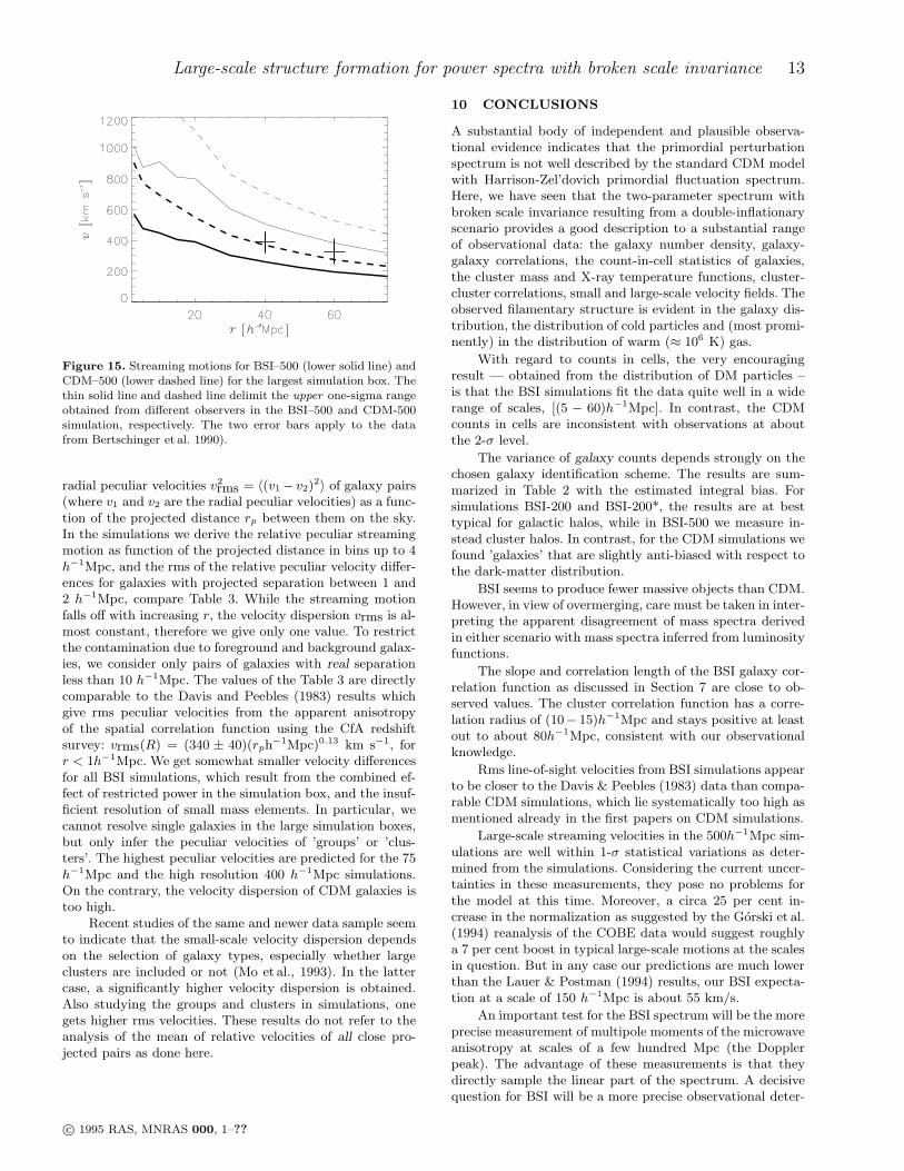
spheres considered there is of course some overlap in thelarger spheres.) The results of the 500 h−1Mpc simulationare shown in Fig. 15. Bertschinger et al. (1990) estimatedthe average velocities of the mass within spheres of radius40 and 60h−1Mpc centered at the Local Group as 388± 67and 327±82 km s−1, respectively (see data points in Fig. 14).At the 1-σ level, these estimates are compatible both withthe BSI results and with CDM. The rms velocities for BSI-200* (not plotted) and BSI-500 are both well fitted by curvesof the form vrms = v0 exp(−x/x0), with v0 ≈ 490 km s−1,x0 = 41.7h−1Mpc for simulation BSI-200*, and v0 ≈ 520km s−1, x0 = 66.7h−1Mpc for simulation BSI-500. The min-imum mass included in the catalogs was 2.6×1011M⊙ for thehigh-resolution simulation BSI-200*, 2×1011M⊙ for the sim-ulations BSI-200 and CDM-200, and 3×1013M⊙ for the sim-ulations BSI-500 and CDM-500. However, varying the mini-mummass had little effect (i.e., resulted in a shift well withinthe range of statistical uncertainty). The Lauer and Postman(1994) measurement (689 ± 178) km s−1at 150h−1Mpc liesabove the bulk velocity in any of 512 bins for all CDM andBSI simulations at the largest radius computed (75h−1Mpc).

An important property of BSI models as studied inGMS94 is to provide a natural mechanism for a relativelyhigh Mach-number or “cold” flow (Ostriker & Suto 1990,Strauss et al., 1993). Small-scale velocity fields may be stud-ied by measuring the rms line-of-sight relative peculiar ve-locity derived from galaxy catalogs (Turner 1976; Davis &Peebles 1983; Mo et al. 1993).

Davis and Peebles (1983) first inferred the small-scalevelocity field of galaxy clustering from the anisotropy of thesmall-scale velocity dispersion. They derived the rms relative

c© 1995 RAS, MNRAS 000, 1–??


Figure 15. Streaming motions for BSI–500 (lower solid line) andCDM–500 (lower dashed line) for the largest simulation box. Thethin solid line and dashed line delimit the upper one-sigma rangeobtained from different observers in the BSI–500 and CDM-500simulation, respectively. The two error bars apply to the datafrom Bertschinger et al. 1990).

radial peculiar velocities v2rms = 〈(v1− v2)2〉 of galaxy pairs

(where v1 and v2 are the radial peculiar velocities) as a func-tion of the projected distance rp between them on the sky.In the simulations we derive the relative peculiar streamingmotion as function of the projected distance in bins up to 4h−1Mpc, and the rms of the relative peculiar velocity differ-ences for galaxies with projected separation between 1 and2 h−1Mpc, compare Table 3. While the streaming motionfalls off with increasing r, the velocity dispersion vrms is al-most constant, therefore we give only one value. To restrictthe contamination due to foreground and background galax-ies, we consider only pairs of galaxies with real separationless than 10 h−1Mpc. The values of the Table 3 are directlycomparable to the Davis and Peebles (1983) results whichgive rms peculiar velocities from the apparent anisotropyof the spatial correlation function using the CfA redshiftsurvey: vrms(R) = (340 ± 40)(rph

−1Mpc)0.13 km s−1, forr < 1h−1Mpc. We get somewhat smaller velocity differencesfor all BSI simulations, which result from the combined ef-fect of restricted power in the simulation box, and the insuf-ficient resolution of small mass elements. In particular, wecannot resolve single galaxies in the large simulation boxes,but only infer the peculiar velocities of ’groups’ or ’clus-ters’. The highest peculiar velocities are predicted for the 75h−1Mpc and the high resolution 400 h−1Mpc simulations.On the contrary, the velocity dispersion of CDM galaxies istoo high.

Recent studies of the same and newer data sample seemto indicate that the small-scale velocity dispersion dependson the selection of galaxy types, especially whether largeclusters are included or not (Mo et al., 1993). In the lattercase, a significantly higher velocity dispersion is obtained.Also studying the groups and clusters in simulations, onegets higher rms velocities. These results do not refer to theanalysis of the mean of relative velocities of all close pro-jected pairs as done here.

10 CONCLUSIONS

A substantial body of independent and plausible observa-tional evidence indicates that the primordial perturbationspectrum is not well described by the standard CDM modelwith Harrison-Zel’dovich primordial fluctuation spectrum.Here, we have seen that the two-parameter spectrum withbroken scale invariance resulting from a double-inflationaryscenario provides a good description to a substantial rangeof observational data: the galaxy number density, galaxy-galaxy correlations, the count-in-cell statistics of galaxies,the cluster mass and X-ray temperature functions, cluster-cluster correlations, small and large-scale velocity fields. Theobserved filamentary structure is evident in the galaxy dis-tribution, the distribution of cold particles and (most promi-nently) in the distribution of warm (≈ 106 K) gas.

With regard to counts in cells, the very encouragingresult — obtained from the distribution of DM particles –is that the BSI simulations fit the data quite well in a widerange of scales, [(5 − 60)h−1Mpc]. In contrast, the CDMcounts in cells are inconsistent with observations at aboutthe 2-σ level.

The variance of galaxy counts depends strongly on thechosen galaxy identification scheme. The results are sum-marized in Table 2 with the estimated integral bias. Forsimulations BSI-200 and BSI-200*, the results are at besttypical for galactic halos, while in BSI-500 we measure in-stead cluster halos. In contrast, for the CDM simulations wefound ’galaxies’ that are slightly anti-biased with respect tothe dark-matter distribution.

BSI seems to produce fewer massive objects than CDM.However, in view of overmerging, care must be taken in inter-preting the apparent disagreement of mass spectra derivedin either scenario with mass spectra inferred from luminosityfunctions.

The slope and correlation length of the BSI galaxy cor-relation function as discussed in Section 7 are close to ob-served values. The cluster correlation function has a corre-lation radius of (10− 15)h−1Mpc and stays positive at leastout to about 80h−1Mpc, consistent with our observationalknowledge.

Rms line-of-sight velocities from BSI simulations appearto be closer to the Davis & Peebles (1983) data than compa-rable CDM simulations, which lie systematically too high asmentioned already in the first papers on CDM simulations.

Large-scale streaming velocities in the 500h−1Mpc sim-ulations are well within 1-σ statistical variations as deter-mined from the simulations. Considering the current uncer-tainties in these measurements, they pose no problems forthe model at this time. Moreover, a circa 25 per cent in-crease in the normalization as suggested by the Gorski et al.(1994) reanalysis of the COBE data would suggest roughlya 7 per cent boost in typical large-scale motions at the scalesin question. But in any case our predictions are much lowerthan the Lauer & Postman (1994) results, our BSI expecta-tion at a scale of 150 h−1Mpc is about 55 km/s.

An important test for the BSI spectrum will be the moreprecise measurement of multipole moments of the microwaveanisotropy at scales of a few hundred Mpc (the Dopplerpeak). The advantage of these measurements is that theydirectly sample the linear part of the spectrum. A decisivequestion for BSI will be a more precise observational deter-

c© 1995 RAS, MNRAS 000, 1–??


Table 3. First (vstr, defined positive inwards) and second (vrms) moments of distributionof line-of-sight projected relative peculiar velocity differences of galaxy halo pairs.

Simulation vstr [km s−1] vrms [km s−1](0 - 1) (1 - 2) (2 - 3) (3 - 4) (1 - 2)h−1Mpc h−1Mpc h−1Mpc h−1Mpc h−1Mpc

BSI-200* 183 159 142 130 256BSI-25* 50 40 27 18 192BSI-500 176 169 139 106 243BSI-200 141 117 111 101 241BSI-75 106 104 97 88 253BSI-25 82 78 69 62 192CDM-500 362 373 316 266 469CDM-200 224 216 201 172 484CDM-75 204 218 207 199 644CDM-25 100 126 131 110 469

mination of the epoch of formation of the first objects. Asmentioned in Sect. 5, improved treatment of ionization andheating processes could allow use of quasar abundance andquasar absorption line data to obtain more stringent limitson structure evolution in BSI. Of comparable importanceare data expected to be available in the near future on theevolution of the cluster mass function at redshifts z ≈ 0.5.This problem presents a theoretical challenge, because it re-quires an accurate hydrodynamical treatment of cluster gasdynamics in the context of large-scale structure simulations.

The most important success of the BSI scenario is theexcellent agreement with present observational data on verylarge scale structure. In this paper, we have seen throughnumerical simulations that smaller scales are generally inexcellent agreement with available data. In the future, itwill be important to investigate additional characteristics oflarge-scale structure using methods such as topological stud-ies, percolation analysis and computation of void probabilityfunctions.

In order to study mass spectra and statistics in a morereliable manner, hydrodynamic simulations should be per-formed. However, the results of our PM simulations stronglysuggest that the BSI model studied here deserves full at-tention as a reliable description of cosmological structureformation.

Acknowledgements:

We would like to express our thanks to Andrei Dorosh-kevich and Anatoly Klypin for stimulating discussions. Ourreferee, David Weinberg, made a lot of constructive remarkswhich helped us very much in improving the paper. Karl-Heinz Boning provided invaluable support in computer man-agement.

REFERENCES

Amendola, L., Gottlober, S., Mucket, J. P., & Muller, V. 1995,ApJ in press

Bahcall, N. A., & Soneira, R. A. 1983, ApJS, 70, 1Bahcall, N. A., & Cen, R. 1993, ApJ. 407, L49Bartlett, J. G., & Silk, J. 1993, ApJ. 407, L45

Baugh, C. M., & Efstathiou, G. 1993, MNRAS 265, 145Bertschinger, E., Dekel, A., Faber, S., Dressler, A., & Burstein,

D. 1990 ApJ 364, 370

Blumenthal, G. R., Pagels, H., & Primack, J. R. 1982, Nature299, 37

Bond, J. R., & Efsthathiou, G. 1984, ApJ 285, L45

Bond, J. R., 1994, CITA-94-5 (Proceedings of the Capri meeting)

Cen, R., Gnedin, N.Y., Kofman, L. A., & Ostriker, J. 1992, ApJ399, L11

Cen, R., Gnedin, N.Y., & Ostriker, J. 1993, ApJ 417, 387

Cen, R., & Ostriker J. 1992a, ApJ 392, 22

Cen, R., & Ostriker J. 1994, ApJ 431 451

Cen, R. 1004, ApJ 437, 12

Collins, C. A., Cruddace, R. G., Ebling, H., MacGillivray, H. T.,& Voges, W. 1994 in: ’Studying the Universe with clusters ofgalaxies’, eds. H. Bohringer, S. Schindler, MPE Report 256,107

Davis, M., Summers, F. J. & Schlegel, D. 1992, Nature 359, 393

Davis, M. & Peebles, P.J.E. 1983, ApJ 267, 465

Doroshkevich, A. G., Fong, D., Gottlober, S., Mucket, J. P., &Muller, V. 1995 MNRAS submitted

Efstathiou, G., Ellis, R.S., & Peterson, B.S. 1992, MNRAS 232,431

Efstathiou, G. 1992, MNRAS 256, 43P

Efstathiou, G., Bond, J. R., & White, S. 1992, MNRAS 258, 1P

Efstathiou, G., Kaiser, N., Saunders, W., Lawrence, A., Rowan-Robinson, M., Ellis, R.S., & Frenk, C. S. 1990a, MNRAS 247,

10P

Evrard, A.E. 1990, ApJ. 363, 349

Evrard, A.E., Mohr, J.J., Fabricant, D.G., & Geller, M.J. 1993,Astr.J. 95, 985

Fall, S.M., & Rees, M. 1985, ApJ 298, 18

Fisher, K. B., Davis, M., Strauss, M. A. Yahil, A., & Huchra, J.P. 1993, ApJ 402, 44

Gorski, K. M., Hinshaw, G., Banday, A. J., Bennett, C. L.,Wright, E. L., Kogut, A., Smoot, G. F., & Lubin, P. 1994,ApJ 430, L89

Gottlober, S., & Mucket, J. P. 1993, A&A 272, 1

Gottlober, S., Mucket, J. P., & Starobinsky A. A. 1994, ApJ, 434,417, GMS94

Gottlober, S., Muller, V., & Starobinsky, A. A. 1991, Phys. Rev.D43, 2510 GMS91

Gottlober, S. 1994, in: ’Studying the Universe with clusters ofgalaxies’, Ringberg workshop, eds. H. Bohringer, S. Schindler,MPE Report 256, 79

Henry, J. P., & Arnaud, K. A. 1991, ApJ 372, 410

Kaiser, N. 1984, ApJ 284, L9

Kaiser, N. 1991, ApJ 383, 104

Kamionkowski, M. Spergel, D., & Sugiyama, N. 1994, ApJ 426,L57

Kang, H., Ostriker, J.P., Cen, R., Ryu, D., Hernquist, L., Evrard,

c© 1995 RAS, MNRAS 000, 1–??


A.E., Bryan, G.,& Norman, M.L., 1994, ApJ 430, 83

Kates, R., Kotok E., & Klypin, A. 1991, A& A 243, 295 (KKK91)Katz N., & Gunn, J. 1991, ApJ 377, 365Katz N., Hernquist, L. & Weinberg, D. H. 1992, ApJ 399, L109Katz N., & White, S. 1993, ApJ. 412, 455Kauffmann, G., White, S., & Guiderdoni, B. 1993, MNRAS 264,

201Kauffmann, G., & Charlot, S. 1994, ApJ 430, L97Klypin, A., Holtzman, J. Primack. J., & Regos, E. 1993, ApJ 416,

1Klypin, A., & Kates, R. 1991, MNRAS 251, 41P (KK)Klypin, A., Kates, R, & Khokhlov, A. 1992, in: ’New Insights

into the Universe’, Lecture Notes in Physics 171 Springer,157 (KKK92)

Klypin, A., & Kopylov, A. I. 1983, Soviet Astr. Letters 9, 41Kofman, L., Gnedin, N., & Bahcall, N. 1993, ApJ 413, 1.Lauer, T., & Postman, M. 1994, ApJ 425, 418.Lilje, P. B. 1992, ApJ 386, L33Loveday, J., Peterson P., Efstathiou, G., & Maddox, S. 1992, ApJ

390, 338Maddox, S. J., Efstathiou, G., Sutherland, W.J., & Loveday, J.

1990, MNRAS 242, 43Mo, H.J., Jing, Y.P., Borner, G. 1993, in: Borner & Buchert (eds.),

‘Proc. 4. MPG-CAS Workshop on High Energy Physics andCosmology’ MPA/P8

Mo, H.J., & Miralda-Escude, J. 1994, ApJ 430, L25Mucket, J.P., Kates, R., Petitjean, P., & Riediger, R. 1995, in

preparationMuller, V. 1994a, in: ’Cosmological Aspects of X-Ray Clusters of

Galaxies’, NATO ASI Series Vol 441, Kluwer, 439Muller, V. 1994, in: ’Studying the Universe with clusters of galax-

ies’, Ringberg workshop, eds. H. Bohringer, S. Schindler, MPEReport 256, 85

Navarro, J. F., & Benz, W. 1991, ApJ 380, 320Ostriker, J. 1993, Ann. Rev. Astron. Astrophys. 31, 689Ostriker, J., & Suto 1990, ApJ 348, 378Park, C., Gott, J., & da Costa, L. 1992, ApJ 392, L51Petitjean, P., Mucket, J. P., & Kates, R. 1995, A&A 295, L9Press, W. H., & Schechter, P. 1974, ApJ 187, 425Shapiro, P., & Struck-Marcell, C. 1985, ApJ Suppl 57, 205Smoot, G. F. et al. 1992, ApJ 396, 1Starobinsky, A. A., 1985, JETP Lettt. 42, 152Steinmetz, M., & Muller, E. 1995, MNRAS in pressThoul, A.A., & Weinberg, D.H. 1994, preprint astro-ph/941000Turner, E. L. 1976, ApJ 208, 20Vogeley, M. S., Park, C., Geller, M., & Huchra, J. P. 1992, ApJ

391, L5

White, S., Frenk, C. S., Davis, M., & Efstathiou, S. 1987, ApJ313, 505 MNRAS 258, 1P

White, S., Navarro, J. F., Evrard, A. E., & Frenk, C. S. 1994,Nature 366, 429

Zel‘dovich, Y. B. 1970, A&A 5, 84

c© 1995 RAS, MNRAS 000, 1–??

large-scale structure formation for power spectra with ... · large-scale structure formation for...

Documents