Working Paper/Document de travail 2015-21

Large-Scale Asset Purchases: Impact on Commodity Prices and International Spillover Effects

by Sharon Kozicki, Eric Santor and Lena Suchanek

2

Bank of Canada Working Paper 2015-21

June 2015

Large-Scale Asset Purchases: Impact on Commodity Prices and International

Spillover Effects

by

Sharon Kozicki, Eric Santor and Lena Suchanek

Bank of Canada

Ottawa, Ontario, Canada K1A 0G9 Corresponding author: ESantor@bankofcanada.ca

Bank of Canada working papers are theoretical or empirical works-in-progress on subjects in economics and finance. The views expressed in this paper are those of the authors.

No responsibility for them should be attributed to the Bank of Canada.

ISSN 1701-9397 © 2015 Bank of Canada

ii

Acknowledgements

The authors would like to thank David Laidler (University of Western Ontario and C.D. Howe Institute), participants at the “Zero Bound on Interest Rates and New Directions in Monetary Policy 2011” conference in Waterloo and the “Birmingham Econometrics and Macroeconomics Conference 2012,” and seminar participants at the Bank of Canada and the Bank of England for useful comments.

iii

Abstract

Prices of commodities, including metals, energy and agricultural products, rose markedly over the 2009–2010 period. Some observers have attributed a significant part of this increase in commodity prices to the U.S. Federal Reserve’s large-scale asset purchase (LSAP) programs. Using event-study methodologies, this paper investigates whether the announcement and subsequent implementation of the Fed’s LSAPs, and communication of the tapering of these purchases, affected commodity prices. Our empirical results suggest that LSAP announcements did not lead to higher commodity prices. However, there is some evidence that the currencies of commodity exporters appreciated and that their stock markets posted gains. The results suggest that other factors, such as supply constraints and robust demand from emerging-market economies, were the likely drivers behind the increase in commodity prices. Last, the paper finds that commodity prices have become more sensitive to macroeconomic news when monetary policy is at the effective lower bound.

JEL classification: E58, G14, Q00 Bank classification: International topics

Résumé

Les cours des matières premières, dont les métaux, l’énergie et les produits agricoles, ont connu une forte hausse entre 2009 et 2010. Certains observateurs ont attribué une part importante de cette augmentation aux programmes d’achat massif d’actifs pilotés par la Réserve fédérale américaine. L’objet de notre étude est d’évaluer, au moyen de méthodes appliquées aux études événementielles, si les cours des matières premières ont été influencés par l’annonce et la mise en œuvre de ces programmes, ainsi que par l’annonce de la normalisation du rythme d’achat des actifs. Au vu des résultats empiriques, tout porte à croire que les annonces n’ont pas entraîné de renchérissement des matières premières. Il y a néanmoins lieu de penser que les devises des exportateurs de matières premières se sont appréciées, et que les marchés boursiers ont enregistré des gains. D’autres facteurs, qu’il s’agisse de contraintes liées à l’offre ou de la demande robuste des pays émergents, auraient donc fait monter les prix des matières premières. Enfin, les prix des matières premières sont plus sensibles aux nouvelles macroéconomiques depuis que le taux directeur se situe à sa valeur plancher.

Classification JEL : E58, G14, Q00 Classification de la Banque : Questions internationales

iv

Non-Technical Summary Motivation and Question

The Great Recession provoked an unprecedented policy response from the U.S. Federal Reserve, including the implementation of quantitative easing (QE). Although most observers agree that QE has been successful, some have criticized the programs for having significant spillover effects, for instance on commodity prices. While the appreciation of commodity prices over the 2009–2010 period can largely be explained by fundamentals, it is nevertheless important that central banks understand to what extent QE may have contributed to this development. In our paper, we investigate whether the announcement and implementation of QE programs, as well as communication related to the eventual exit from the last round of purchases, affected commodity prices.

Methodology

To identify the effect of QE, we conduct two types of event studies. That is, we examine movements in commodity prices, as well as commodity-exporter stock market indexes and currencies, on days when the Fed publicly announced intended or actual asset purchases. The rationale for focusing on a short time window surrounding the announcement is that forward-looking financial markets should quickly incorporate all information from a public announcement shortly after the announcement is made.

Key Results and Contributions

Overall, we do not find any evidence that QE led to a rise in the prices for metals, energy and agricultural commodities. In fact, oil prices tended to fall on announcement dates, particularly with QE1. The results suggest that other factors, such as supply constraints and improving demand on the back of the global recovery, were most likely the primary drivers behind the increase in commodity prices. Nevertheless, results suggest that QE did have spillover effects on commodity-producing countries. Indeed, commodity-exporter currencies tended to appreciate upon QE announcements, while commodity-exporter stock markets posted gains. This suggests that while investors might not have reacted to QE by directly investing into commodities, they may have increased their exposure to commodities by investing in commodity-related assets such as commodity currencies and commodity-heavy equity markets. Last, we find that commodity prices appear to have become more responsive to macroeconomic shocks during the periods covered by QE policies, when compared with the pre-recession period. Positive macroeconomic surprises tend to be associated with higher oil prices during periods when monetary policy is at the effective lower bound.

Future Work and Comments

Several possible extensions are left for future work. First, it would be interesting to construct a measure of the surprise element of QE announcements. Second, one caveat about event studies is that they cannot estimate the duration impact of QE announcements. Whether QE had a permanent impact on commodity-exporter stock markets and currencies is beyond the scope of our research, but would be worthwhile to address through alternative models.

1

1. Introduction In response to the global financial crisis and subsequent Great Recession, the U.S. Federal Reserve Board (the Fed) responded aggressively, lowering its policy rate to near zero and engaging in a wide array of “unconventional” monetary policies. In particular, it implemented large-scale asset purchases (LSAPs) of Treasury securities, as well as mortgage-backed securities and agency debt (often referred to as quantitative easing, or QE), in order to lower long-term interest rates and stimulate economic activity. As the recovery showed renewed weakness in 2010, a second round of LSAPs (QE2) was announced. With sovereign debt concerns in Europe and ongoing weakness in the U.S. labour and housing markets weighing on economic activity, the Fed announced further LSAPs in September 2011 (this time sterilized by sales of its short-term debt holdings) and open-ended purchases in September 2012. Over the summer of 2013, the Fed discussed reducing monthly purchases, and announced the first reduction in December 2013, beginning in January 2014.

The initial assessments of the effectiveness of these policies have been largely positive.1 However, some observers have argued that exceptionally accommodative monetary policy also has significant spillover effects, including contributing to an increase in capital flows to emerging-market economies (EMEs), a depreciation of the U.S. dollar and rising commodity prices.2 Indeed, commodity prices (as measured by the Thomson Reuters/Jefferies CRB Index) rose 42 per cent throughout 2009 following the implementation of the first round of LSAPs, and surged another 37 per cent between the Jackson Hole speech in August 2010 and the end of March 2011 (i.e., the second round of LSAPs) (Chart 1). The increase in commodity prices appeared to be broad based, with oil and metals prices rising from early 2009 onwards, and agricultural prices gaining momentum from late 2010 (Chart 2).

While this widespread run-up in the prices of crude oil and other commodities can largely be explained by fundamentals (Murray 2011), it is nevertheless important that central banks understand to what extent unconventional monetary policy may have contributed to higher commodity prices. In particular, rising energy and food prices can feed both directly and indirectly into higher inflation. Moreover, for energy importers, the rise in oil prices restrains consumer spending and weakens confidence, and is thus a potential drag on the recovery.

Despite the often-elevated rhetoric with respect to the spillover effects of quantitative easing on commodity prices, there is surprisingly little empirical evidence to support (or deny) these claims. Glick and Leduc (2012) study the response of commodity prices on announcement

1 For a review, see Santor and Suchanek (2013). 2 For instance, see Reinhart (2011).

2

dates; they find that commodity prices actually fell, on average, around LSAP announcement dates.

In our paper, we use two different event-study methodologies to empirically investigate whether the announcement of LSAPs, their subsequent implementation and the communication of the eventual exit from QE3 affected commodity prices. Detecting the effects of LSAPs on commodity prices, however, may be complicated by (i) specific supply and demand factors, or (ii) the fact that commodity assets are not easily accessible to a broad class of investors. To this end, we also explore the effect of LSAPs on equity markets and exchange rates in commodity-producing countries. Last, we study whether the sensitivity of commodity prices to macroeconomic news has changed during periods where monetary policy is at the effective lower bound.

We come to three main conclusions:

(i) LSAPs do not appear to have had a measurable abnormal effect on overall commodity price movements. In fact, no consistent pattern emerges when the prices for metals, energy and agricultural commodities are examined. The results appear to be robust to the methodology or specification of the model.

(ii) LSAPs appear to have had positive spillover effects on the currencies and stock markets of commodity exporters, including Australia, Brazil, Canada, Mexico, New Zealand, Norway and South Africa.

(iii) Commodity prices appear to have become more responsive to macroeconomic shocks during the periods covered by LSAPs, when compared with pre-LSAP periods. Positive macroeconomic surprises tend to be associated with higher oil prices during periods when monetary policy is at the effective lower bound.

Overall, our results suggest that, while other factors, such as supply constraints and ongoing demand growth from EMEs were the primary drivers behind the increase in commodity prices since 2009, LSAPs did have spillover effects on commodity-exporting countries.

The paper proceeds as follows: Section 2 examines the channels through which monetary policy may affect commodity prices. Section 3 introduces the event-study methodology and the data. Section 4 presents the estimated impact of LSAPs on commodity prices. Section 5 estimates the impact of LSAP-related announcements on the currencies of commodity exporters, as well as on their broad and energy-specific stock market indexes. Section 6 examines the impact of surprises in macroeconomic announcements on oil prices and Section 7 concludes.

3

2. Monetary Policy and Commodity Prices There are five main transmission channels from monetary policy to commodity prices.

(i) Portfolio reallocation: The primary objective of LSAPs is to reduce long-term Treasury yields. A fall in yields would lead to a reallocation of investors’ portfolios, under the hypothesis that different assets are imperfect substitutes (portfolio-balance channel). In particular, investors would sell Treasuries and purchase other, riskier assets, including commodities, resulting in higher prices (Glick and Leduc 2012).

(ii) Inventory demand: Lower interest rates would, ceteris paribus, increase inventory demand for commodities because the cost of carrying inventories decreases. This in turn would lead to a rise in the spot prices of storable commodities.

(iii) Exchange rate depreciation: Commodity prices may be affected indirectly via exchange rates. An easing of U.S. monetary policy is generally associated with a weakening U.S. dollar. Commodities, most of which are priced in U.S. dollars, would become more affordable for holders of other currencies, thus increasing demand and prices.

(iv) Supply restrictions: Low interest rates may lead oil-producing countries to keep crude in the ground if the returns from pumping oil and investing the proceeds at low interest rates are lower than the return to leaving it in the ground. This decrease in supply, together with higher demand, would contribute to a rise in oil prices (Frankel and Rose 2010).3

(v) Economic growth: More stimulative monetary conditions should improve economic growth, and thus the demand for commodities.

While these transmission channels would suggest that lower interest rates are associated with a rise in commodity prices, LSAPs may cause commodity prices to fall through other channels. For instance, LSAP announcements may signal that policy-makers perceive that the outlook has become weaker. In this case, market worries about the economic outlook may lead investors to increase their demand for safe Treasuries, lowering their yields. If investors simultaneously reduce their demand for risky assets, such as commodities, prices would fall (Glick and Leduc 2012). Thus, how LSAP announcements affect commodity prices depends crucially on underlying financial and economic conditions at the time of the announcement. For example, Kozicki, Santor and Suchanek (2011) argue that the magnitude of the effects of the Federal Reserve’s second round of LSAPs on financial markets may have been more modest than the first round of purchases, which was implemented at a time of considerable strain in financial markets, severely weakened macroeconomic conditions and low confidence. Consequently, the

3 However, anecdotal evidence does not suggest that firms behave in a manner consistent with this hypothesis.

4

reaction of commodity prices has likely been different during the pre- and post-LSAP periods ̶ a question that we will analyze in turn.

The impact on commodities may not just be limited to commodities themselves. If the transmission mechanism of LSAPs works as suggested by the portfolio-rebalancing effect, we would expect to see investors move into commodity currencies other than the U.S. dollar. That is, if investors wanted to get exposure to commodities without investing directly in commodities, they could do so by investing in either commodity-heavy equity markets or commodity currencies. Importantly, commodity-exporter currency and stock markets remained liquid throughout the crisis, and thus provide an appropriate testing field to study the international spillover effects of LSAPs. Thus, our analysis includes the reaction not only of commodity prices themselves, but also of commodity-exporter currencies and stock price indexes.

3. Event-Study Methodology and Data This section briefly describes the event-study approach, explains the two different methodologies, and introduces the relevant data and event dates.

3.1. Event-study approach

Assessing the financial market impact of LSAPs is complicated by many conceptual and empirical hurdles, especially those related to identification (Kozicki, Santor and Suchanek 2011). For example, gauging the effectiveness of individual measures is complicated by numerous identification issues, including:

(i) Contemporaneous measures and effects: The impact of asset purchases on longer-term interest rates may be difficult to gauge, owing to contemporaneous financial sector and macro-policy initiatives, and macroeconomic developments.

(ii) Ongoing nature of the crisis: While many central banks have exited from some unconventional policies, the effects of the crisis (or for that matter, the evolution of the crisis from a financial crisis to a sovereign-debt crisis) are still being felt and some unconventional policies are either still in place or have been expanded.

(iii) Policy lags: Certain measures might have affected markets with a long lag, owing to uncertainty about the features of the measure, skepticism regarding its implementation, and the nature of the transmission mechanism.

(iv) Fiscal policy: Unconventional monetary policies and extraordinarily low interest rates may have amplified the effects of fiscal policy.

To identify the effect of LSAPs, we conduct two types of event studies on movements in commodity prices on “announcement dates,” i.e., days when the Fed publicly announced intended or actual asset purchases. The rationale for this approach is that forward-looking

5

financial markets should quickly incorporate all information from a public announcement shortly after the announcement is made. Intuitively, financial markets would not be expected to forgo large, riskless, profitable trading opportunities for more than a few days or even hours, and thus the impact would be reflected in prices within a short period of time following the announcement. Another advantage of event-study analysis over lower-frequency regression is that it holds other fundamental drivers of commodity prices, such as supply shocks, essentially constant. Simply, by considering changes in commodity prices across a two- or three-day window surrounding the announcement, fundamentals (beyond those associated with the announcement itself) can be argued to have changed very little.4 Event studies would also appear to avoid endogeneity problems that can arise when monthly or quarterly data are used, which can make estimating the effects of LSAPs difficult.

Previous studies have used the event-study approach to estimate the impact of announcements on asset prices. For example, Swanson (2011) uses an event-study analysis to estimate the impact of the “Maturity Extension Program,” as well as QE2, on Treasury yields. Some studies have analyzed the impact of news on commodity prices, but few studies have used an event study to do so (see for instance Roache and Rossi 2009).5 Glick and Leduc (2012) use an event study to estimate the impact of LSAP on global financial and commodity markets.

3.2. Event-study methodology

There are two types of event studies. The first involves regression methods where the impact of an event is estimated as a coefficient of a dummy variable that corresponds to each event date. The second approach, the constant mean- or the market-return model, measures abnormal returns as prediction errors from some benchmark model of normal return.

As for the first approach, we use a GARCH(1,1) model6 to regress the return 𝑅𝑖 of commodity i (or the daily change in) and explanatory variables 𝑋𝑖𝑡 and a dummy variable 𝑍𝑡that takes the value one on days of major announcements:

𝑅𝑖𝑡 = 𝛼𝑖 + 𝛽𝑖𝑍𝑡 + 𝛽𝑖𝑋𝑖𝑡 + 𝜀𝑖𝑡. (1)

4 Swanson (2011) argues that this requires that no other major macroeconomic data surprises or announcements occur on the same day as the respective announcement. We are in the process of verifying this assumption by analyzing macroeconomic and commodity market related news for LSAP announcement dates. Swanson (2011) further notes that quarterly regression models have residual standard errors that are too large to detect small, but statistically significant, effects of announcements even if the model is correctly specified and the size of those effects is correctly estimated. 5 Likewise, McKenzie, Thomsen and Dixon (2004) analyze the statistical performance of event-study approaches using daily commodity futures returns data. 6 McKenzie, Thomsen and Dixon (2004) argue that this model is the most powerful when compared with OLS and other GARCH specifications.

6

Note that this approach simply estimates whether the return increased or decreased in a statistically significant way on days of announcements, rather than estimating an abnormal return. Such a response may not indicate that LSAPs had an impact on commodity prices over and above normal market functioning, but simply reflects responses in line with other financial variables such as interest rates. Thus, to determine whether LSAPs disproportionately affected commodity prices or had abnormal international spillover effects, we use the second approach, which estimates the abnormal return of financial variables in response to LSAPs.

Event studies of the second type typically proceed in three steps. First, a model is used to calculate the normal return of a commodity over the event window,7 i.e., the return that would be expected if the event did not take place. We use two types of models to calculate normal returns: a market-price model and a constant-mean-return model. The market-price model assumes a stable linear relationship between the market return and the commodity return, i.e., the return 𝑅𝑖 of commodity i is modelled as a function of the market return 𝑅𝑚, where t denotes time:

𝑅𝑖𝑡 = 𝛼𝑖 + 𝛽𝑖𝑅𝑚𝑡 + 𝜀𝑖𝑡. (2)

The constant-mean-return model assumes that the mean return of a given commodity is constant through time, i.e.:

𝑅𝑖𝑡 = 𝑅_𝚤���� + 𝜀𝑖𝑡. (3)

The respective model is estimated over the estimation window (we use an estimation window of 30 days prior to the event).8 The model can then be used to calculate the normal return 𝐸[𝑅𝑖𝑡|Xit] over the event window, where Xit is the conditioning information, i.e., the market return or the mean return, respectively.

Second, the abnormal return can be calculated for each commodity i and event date. The abnormal return 𝜀𝑖𝑡∗ is defined as the actual ex post return 𝑅𝑖𝑡 of the commodity over the event window minus the normal return:

𝜀𝑖𝑡∗ = 𝑅𝑖𝑡 − 𝐸[𝑅𝑖𝑡|𝑋𝑖𝑡]. (4)

In a final step, we test whether the abnormal return on the dates of the events (or the cumulative abnormal return over the event window) is statistically significant. The null hypothesis for our analysis is that announcements related to LSAPs had no effect on commodity

7 The event window refers to the period over which the commodity prices will be examined, e.g., the day before the announcement to the day after the announcement. We use an event window of five days around the actual event, which implies that the effects of LSAPs on commodity prices are less likely to be contaminated by other important news that could move prices. 8 Under the assumption that commodity returns are jointly multivariate normal and independently and identically distributed through time, the model can be estimated using ordinary least squares. The length of the window is varied in our sensitivity analysis.

7

returns.9 A failure to reject the null hypothesis would suggest that there is no evidence that LSAP announcements caused commodity returns to fall or increase.

3.3. The data

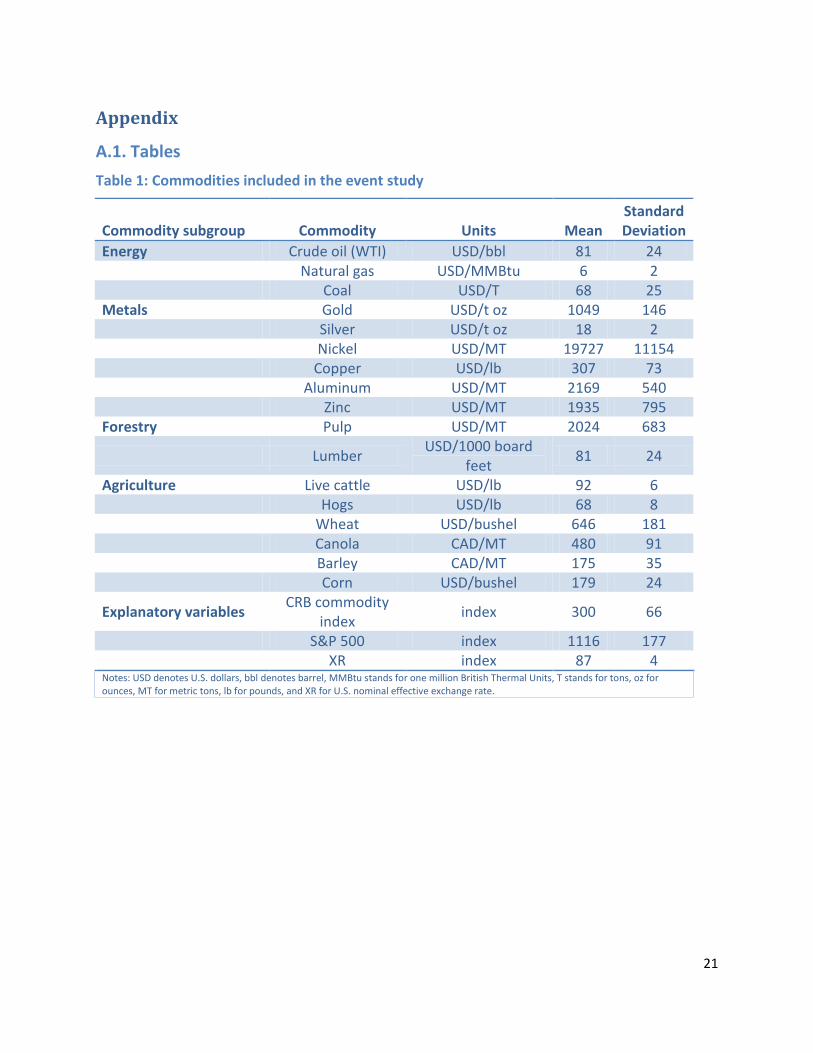
We use data for the 17 major commodities included in the Bank of Canada commodity price index (BCPI) for which price data on commodity futures contracts are available over the period from January 2008 to January 2014 from Bloomberg. The commodities examined include energy, metals, forestry and agricultural commodities (see Table 1 for details). Futures prices are taken from the nearest contract used as the benchmark for that commodity, most of which are traded on exchanges in the United States. For oil prices, we use the West Texas Intermediate (WTI) price, which is the benchmark oil price in the United States.10

Following Roache and Rossi (2009), we focus on the futures market rather than the spot market, for two reasons. First, the spot market for some commodities, including certain precious and base metals, is dominated by trading in London, which means that official fixing prices have less time to respond to daily developments in the United States owing to the five-hour time difference. Second, spot prices are often positively correlated with futures prices with a one-day lag, which indicates that the impact of U.S. announcements on the futures price is likely to affect the spot price the following day. This is consistent with previous research indicating that commodities futures markets lead developments in spot markets (e.g., Antoniou and Foster 1992; Yang, Balyeat and Leatham 2005). We use daily data which appear to better capture the reaction of markets to news, rather than intraday data (Payne 2003). Last, following the event-study literature, we use the log change of commodity prices (i.e., the return) to measure announcement effects.

To assess international spillover effects on commodity-exporting countries, we use the bilateral exchange rates of commodity exporters vis-à-vis the U.S. dollar (including Australia, Brazil, Canada, Mexico, Norway, New Zealand and South Africa), broad stock price indexes of those countries, as well as energy stock indexes and metal stock indexes where available.11

The non-event-related explanatory variables used in the GARCH model and as market-return variables in the market-return model include daily returns on the Commodity Research Bureau (CRB) futures price index, daily returns on the Standard and Poor’s (S&P) 500 stock market index, and the JPMorgan broad nominal U.S. effective exchange rate (i.e., the U.S. nominal trade-weighted exchange rate). The CRB index tracks movements in both nearby and deferred

9 H0: The event had no impact, i.e. 𝜀𝑖𝑡∗ =0, or ∑ 𝜀𝑖𝑡∗𝑒𝑣𝑒𝑛𝑡𝑑𝑎𝑡𝑒+2

𝑒𝑣𝑒𝑛𝑡𝑑𝑎𝑡𝑒−2 =0 for the cumulative abnormal return. 10 One might argue that WTI prices have diverged from Brent oil prices as an increase in Cushing stocks dampened WTI crude prices. However, using the Brent benchmark instead of WTI does not significantly change our results. 11 As a control, we also run regressions on non-commodity currencies, including the Swiss franc, the euro, the yen and the British pound. Future work will include the interest rate differential.

8

futures contracts for 19 commodities.12 It is important to note that 9 of the 17 commodities examined here are included in the CRB index and, hence, there is a potential simultaneity problem.13 Thus, for these commodities, only the S&P market index and the U.S. nominal effective exchange rate are used as explanatory and market-return variables. In contrast, model specifications for the remaining eight commodities include the CRB index, nominal exchange rate, and the S&P market index as explanatory and market-return variables, respectively.

The inclusion of exchange rates and a stock market index is intended to capture the correlation of commodity prices to other financial variables. For example, LSAP announcements may exert an indirect influence through a commodity’s role as an effective hedge against lower interest rates or a depreciating U.S. dollar. In that case, the sensitivity of commodity prices to announcements would merely reflect a relationship between the commodity and other financial assets, rather than the announcements themselves. Indeed, there is strong evidence that commodity prices have been sensitive to the U.S. dollar over a long period. Following Roache and Rossi (2009), we assume that the causality runs from the U.S. dollar to the commodity price, as recent evidence suggests that exchange rates play the dominant role as a forcing variable.14

3.4. Event dates

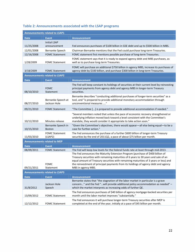
The impact of QE on commodity prices may be measured on days when Fed officials hinted at possible future purchases, as well as firm statements of planned purchases, including time frames and quantities (Neely 2010). Several FOMC statements and speeches also discussed the objectives and the assessment of LSAPs. Gagnon et al. (2010) suggest that there are eight events/announcements associated with the first round of LSAPs that had potentially important information, while Glick and Leduc (2012) suggest six event dates related to the second round of LSAPs (see Table 2 in the Appendix for more details); we add three more events for the Maturity Extension Program (MEP) announced in 2011, three dates for LSAP3 in 2012, and four dates in 2013 for the mention and implementation of a tapering of purchases, i.e., the start of the exit from LSAPs.

LSAPs: Phase 1

On 25 November 2008, the Fed first announced purchases of GSE debt and mortgage-backed securities (MBS), and on 1 December 2008, Chairman Bernanke first hinted at the purchase of

12 Aluminum, cocoa, coffee, copper, corn, cotton, crude oil, gold, heating oil, lean hogs, live cattle, natural gas, nickel, orange juice, silver, soybeans, sugar, unleaded gas and wheat. 13 Ramsey’s (1969) regression specification error test is used to determine whether the inclusion of the return on the CRB index is appropriate for the regression models. Test results indicate that a potential simultaneity problem does exist for regressions using the corn futures returns series. 14 Augmented Dickey-Fuller (ADF) tests indicate that each futures returns series and the three market index returns series are stationary and, hence, equations (1-2) are estimated in the levels of the data.

9

longer-term Treasury securities. The anticipation of LSAPs was further reinforced in the 16 December 2008 FOMC press release. However, the FOMC disappointed markets because it did not announce any concrete purchases in the 28 January 2009 FOMC statement. Purchases of Treasury securities and an extension of mortgage-related securities were finally announced on 18 March 2009.15

LSAPs: Phase 2

The second phase of LSAPs began with the FOMC statement of 10 August 2010, when the Fed announced that it would roll over its holdings of agency securities as they matured into Treasuries, thus avoiding a reduction in the Fed’s balance sheet. Chairman Bernanke’s Jackson Hole speech on 27 August 2010 further reinforced market expectations of renewed purchases, which were finally announced on 3 November 2010.16

Maturity Extension Program (MEP)

The third round of purchases, announced in 2011 (sometimes referred to as “Operation Twist”), differed from the first two because the purchases of longer-dated government debt were “sterilized” by the sale of an equal amount of shorter-term debt in the Fed’s Treasury portfolio. However, given that the short end of the yield curve was anchored at close to zero per cent because the Fed, in August 2011, had committed to hold rates low until mid-2013, the yield curve again flattened (and did not “twist” as would have been the case without anchoring the short end), similar to the effect of LSAP1 and LSAP2.

In terms of the timeline, the Fed’s commitment in August 2011 to keep rates low until mid-2013, including its hint at further easing, can be interpreted as a first announcement of MEP. The minutes of 30 August 2011 show that FOMC members discussed further options for easing. Finally, sterilized LSAPs were announced in September 2011.

LSAPs: Phase 3

The third round of outright purchases was designed as open-ended monthly purchases of MBS and Treasury securities. Bernanke first hinted at additional QE in a speech in Jackson Hole in August 2012, which was implemented shortly thereafter in September, and expanded in December 2012.

15 Over the course of 2009, there were three announcements related to slower or reduced purchases: on 18 August and 23 September 2009, the Fed announced that the pace of Treasury purchases and mortgage-related securities, respectively, would be reduced, followed by the announcement of a slight reduction in the total amount of agency debt to be purchased on 4 November 2009. In this paper, for 2008-2009 we focus on the announcements that would typically be associated with an increase in asset purchases. 16 We further consider three more dates related to the QE2 announcement, which are also considered in Glick and Leduc (2012): the FOMC statement (9/21/2010), the Minutes release (10/12/2010) and the Fed Chairman’s speech, Boston (10/15/2010).

10

The exit

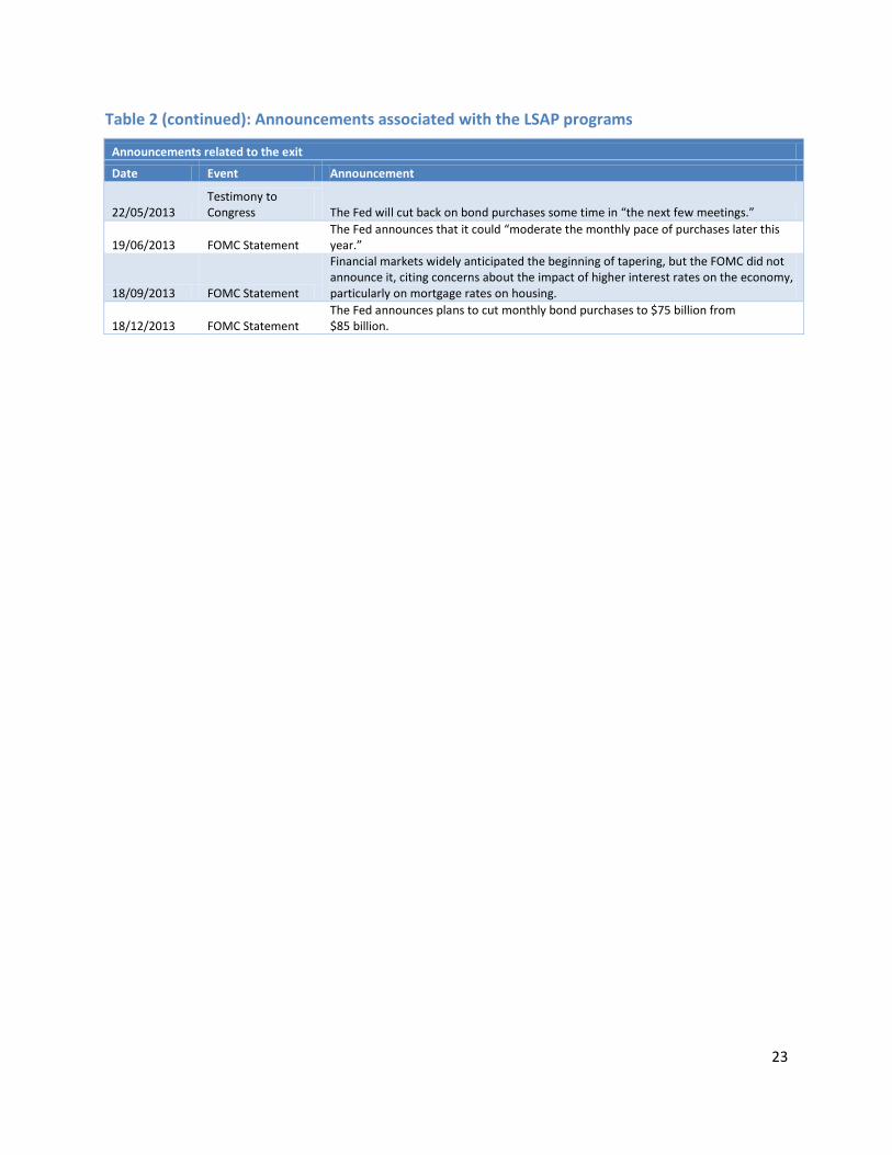
As the labour market improved and the effects of fiscal restraint on the U.S. economy were less severe than expected in 2013, the Fed hinted at an eventual “tapering,” i.e., a reduction in the pace of purchases. In May and June, it explicitly stated that the pace of purchases would be reduced some time during “the next few meetings.” These events may be interpreted as the beginning of an exit policy, followed by the actual first reduction of purchases in January 2014. We refer to these events as “the exit.”

4. Results This section first discusses the estimated impact of LSAP events on commodity prices, as estimated using the dummy regression, followed by results from the mean-return and market-return model.

4.1. Regression analysis using dummy variables

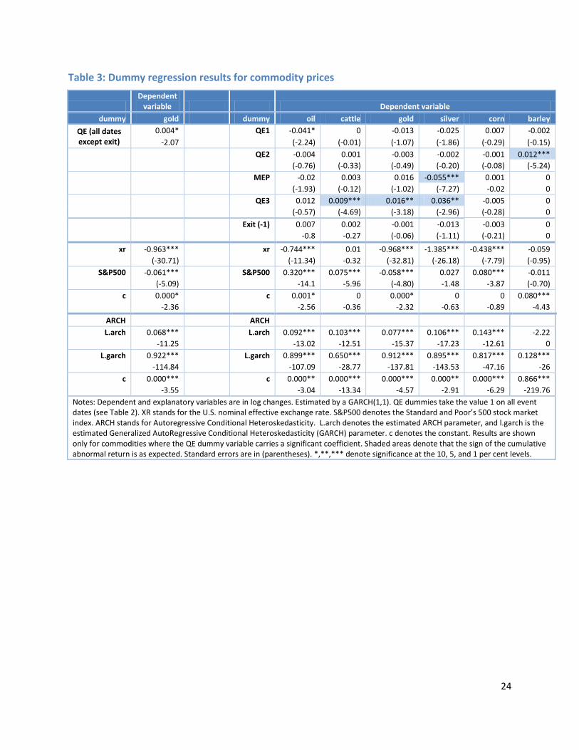
Table 3 shows results for the GARCH(1,1) regression of log changes in commodity prices on one dummy variable for all QE events (first two columns) and on separate dummies (last seven columns) for QE1, QE2, MEP, QE3, and the exit. Of all the commodities, only the response of gold prices on QE announcement days is positive and statistically significant (although it is small). Separating QE events shows that this result is driven by a strong (positive) response on QE3 events. On the other hand, oil prices actually decreased on QE1 events. Overall, only a few commodities other than gold show a statistically significant positive response, including silver (decreasing on MEP events, but increasing on QE3 events), cattle and barley. Results thus far do not suggest that LSAPs led to an overall increase in commodity prices.

We also include dummies for the exit, since if the announcement of purchases is claimed to have led to an increase in commodity prices, the announcement of a reduction of purchases, which can be interpreted as a first step toward an exit from QE, should have led to a fall in commodity prices. Results for events where the Fed mentioned the “tapering” of purchases do not suggest that tapering had an impact on commodity prices. Corn prices increased, but all other responses are not statistically significant. Results are robust to the specification, e.g., using standard OLS regression or using return changes as dependent and explanatory variables (not shown).

The fact that we do not find a consistently positive response of commodity prices on QE announcement dates could be related to the challenge that the announcement of QE may have two effects working against each other: first, QE announcements may be taken as a sign that economic conditions were worse than previously anticipated, and this could dominate the positive effect of QE (Glick and Leduc 2012). Second, lower interest rates implicitly lower the costs of holding commodity inventories and would thus raise demand and prices. While the first

11

effect would lead to weaker commodity prices, the second would lead to stronger commodity prices, thus partially offsetting each other. In addition, if QE, as intended, affects interest rates further out the yield curve, then it is possible that these interest rates are less relevant for financing commodity inventories, suggesting that there might not be an effect on spot commodity prices.

Mean-return and market-return model

This section presents results from the event study using a mean-return and market-return model for each round of the LSAPs.

LSAP: Round 1

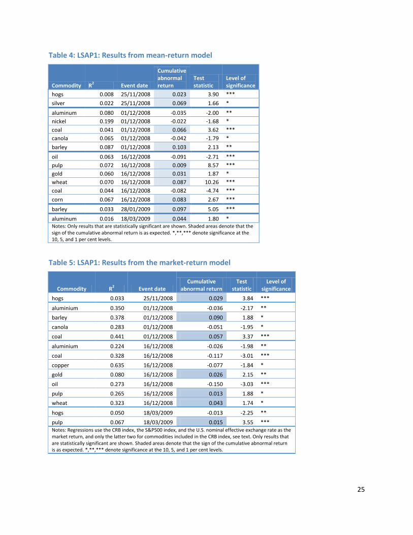
Table 4 shows the R2 from the mean-return regression, the cumulative abnormal return, the two-sided t-test statistic, and the level of significance for each commodity-event combination for the mean-return model using the CRB, the S&P500 and the U.S. nominal effective exchange rate. Table 5 shows the results for the market-return model. We show only statistically significant abnormal returns.

The results suggest that LSAPs had no measurable “abnormal” effect on commodity prices for the market-return model: the cumulative abnormal return is significantly different from zero for only 14 out of 80 commodities and events. In seven cases, the abnormal return is positive, but in the remaining seven cases, it is negative. For instance, the fall in oil prices around the 16 December 2008 FOMC is statistically significant in both models (a cumulative fall of 9-15 per cent in oil prices), consistent with results from the dummy variable regression. Coal prices reacted both positively and negatively (increasing on 1 December 2008, but falling on 16 December 16 2008), while gold prices increased on two occasions. For most other commodities, announcements of LSAPs do not appear to have had a measurable effect; no consistent pattern emerges when one looks at agricultural products17 and forestry products. The results are robust to the length of the event window (for instance, estimating the cumulative abnormal return over a three-day window does not change the results materially), the estimation window, and the specification (mean-return versus market-return model using different explanatory variables).

LSAP: Round 2

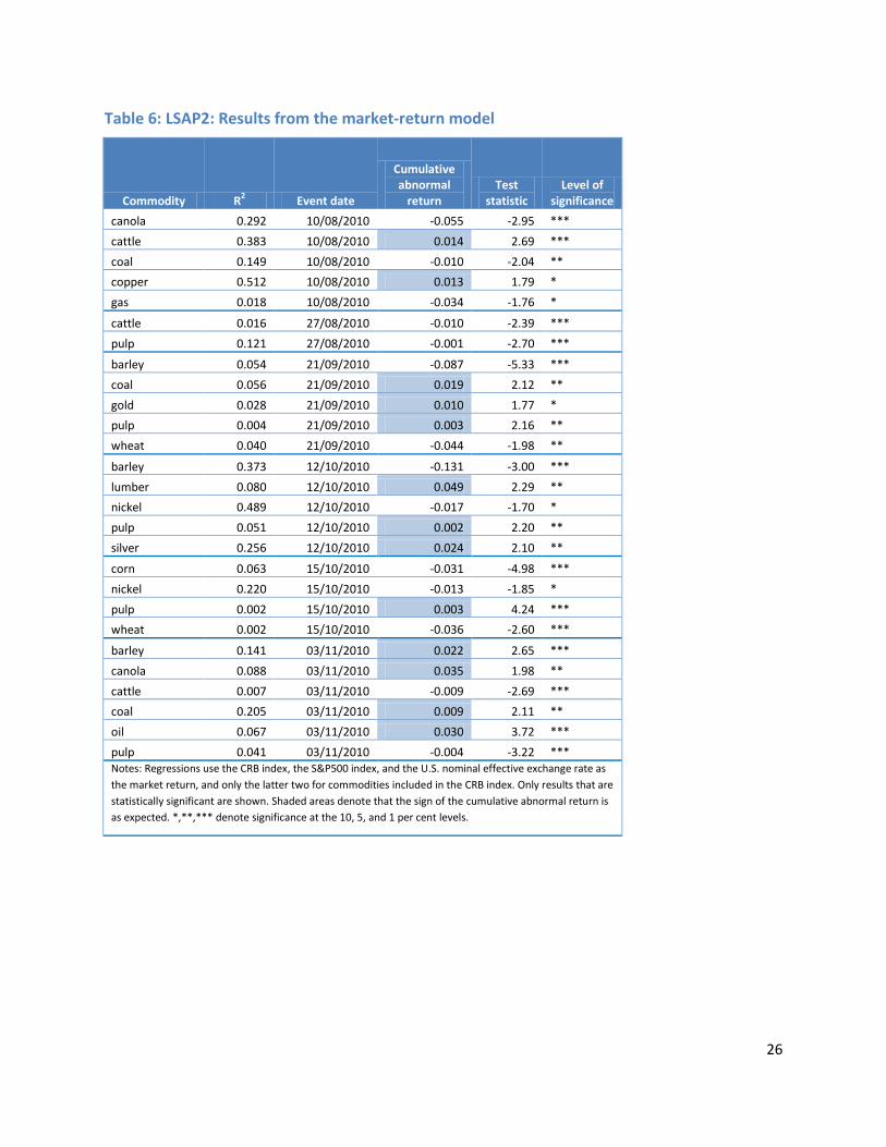
Event-study results for LSAP2, presented in Table 6, suggest that, overall, LSAP announcement dates did not consistently have a significant positive impact on commodity prices. Again, most individual cumulative commodity returns are not statistically different from normal returns (i.e., in 75 out of 97 cases). This result is robust to alternative specifications, i.e., using the mean-

17 For instance, on 16 December 2008, canola prices fell, while wheat prices rose.

12

return model or the market-return model (not shown). A few exceptions stand out: First, the rise in oil prices on 3 November 2010 (a cumulative abnormal return of 3 to 3.5 per cent) is statistically significant, regardless of the specification. Second, natural gas prices fell on the first announcement (cumulative negative abnormal return of 3.4 to 3.8 per cent). A few agricultural commodity price returns show statistically significant abnormal returns, but the pattern is not consistent.18 Overall, about half of the statistically significant abnormal returns are negative. The results are again robust to the length of the event window, the estimation window and the specification.

Chart 3 shows the cumulative abnormal average return for four commodities around the time of the Jackson Hole announcement. In the case of oil and natural gas, the Jackson Hole announcement did not lead to an increase in abnormal returns: at best, they may have mitigated a declining trend. Interestingly, given the very different supply-side conditions affecting these two commodities, and the lack of a clear positive effect, it would seem unlikely that LSAPs were affecting prices significantly. The evidence for wheat reinforces this conclusion, as the announcement did not have any effect. On the other hand, aluminum prices did appear to rebound—however, this may have more to do with demand and supply developments in China, than the stance of U.S. monetary policy.

Maturity Extension Program (MEP)

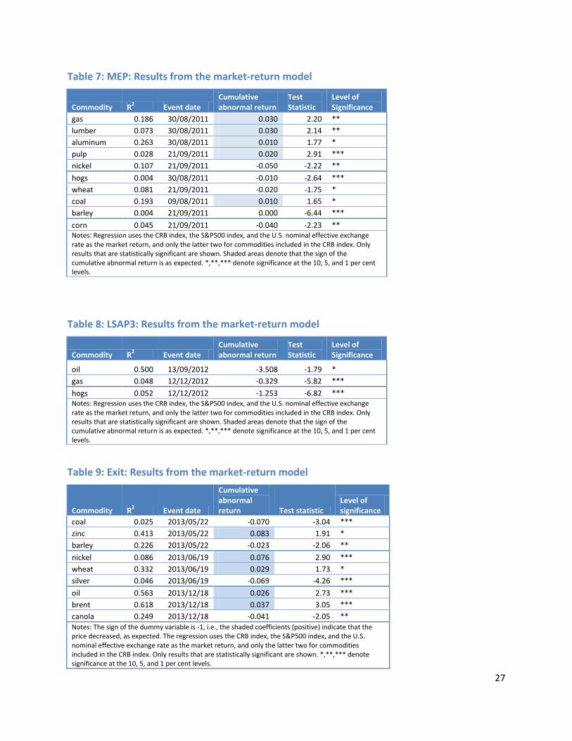
The event-study results for purchases under MEP are presented in Table 7. Again, there appears to be very little evidence that commodity prices reacted in a consistently positive way to LSAP announcements. In particular, only coal prices show a statistically significant abnormal return when the Fed first hinted at another round of easing in its August 2011 statement, whereas other commodity prices did not react. The release of the minutes by the end of August led a statistically significant increase in the prices of some commodities, such as natural gas, but for the actual announcement of MEP in September most statistically significant responses are negative. In sum, the results suggest that LSAP announcements had a significant impact on commodity prices.

LSAP: Round 3

The event-study results for the third round of purchases are presented in Table 8. Again, the impact of purchases appears to become less and less important over time, as commodity prices did not react strongly to LSAP3 announcements. If anything, commodity prices fell on announcement dates, particularly prices for oil, gas and hogs.

18 For instance, corn and wheat prices fell on 15/10/2010, while canola and barley prices increased on the announcement of QE2 (03/11/2010).

13

The exit

Results for the two instances where the Fed hinted at a possible “tapering” of purchases and the day it actually decided to announce the reduction in the pace of purchases are presented in Table 9.19 There is no clear pattern for the response of commodity prices: in four statistically significant cases, commodity prices increased (note that the dummy variable takes the value -1 for exit events, so that a positive coefficient implies a fall), while commodity prices fell in six instances. Oil prices fell on the actual announcement in a statistically significant way, suggesting some evidence that the beginning of the exit led to a decline in oil prices. However, no other commodity prices show a fall on the exit announcement. One explanation might be that while commodity prices fell on the announcement, the S&P index also receded. Thus, the abnormal return, i.e., the movement of commodity prices beyond their correlation with S&P500 and the U.S. nominal effective exchange rate, is not statistically significant, which is to say that commodity prices did not react any more strongly than the usual correlation with other variables would suggest.

Overall, our results are in line with Glick and Leduc (2012). Frankel and Rose (2010), studying the reasons for the run-up in commodity prices until 2008, also find little support for the hypothesis that easy monetary policy and low real interest rates are an important source of upward pressure on real commodity prices, beyond any effect they might have via real economic activity and inflation. The authors conclude that other factors, such as strong demand growth from emerging markets and perhaps speculation, may have contributed to the rise in commodity prices in the 2007‒2008 period. Our results do however not rule out that QE announcements affected financial markets over and above what would be implied by the indirect effects working through real economic activity. As commodities are well financialized, commodity prices, similar to stock markets, reacted to QE announcements, including any impacts on risk premiums, for instance. In this sense, QE announcements triggered a portfolio reallocation, including via commodities, that may have been by more than rational expectations of economic conditions would justify.

Robustness

Several extensions are possible to test the robustness of our results. First, instead of using the one-month futures price, we use 6- and 12-month commodity futures, as well as the spread of 6- and 12-month futures in the event study to capture the potential impact of LSAP on expected commodity prices.20 Results are qualitatively similar to our previous results. For few

19 We also study the impact of the “non-taper” in September 2013, i.e., when the Fed was widely expected to announce the reduction of purchases, but decided to delay the tapering. Results are, however, inconclusive. 20 Data are not available for all commodities at longer horizons. In particular, there are no 12-month futures data for lumber, cattle, hogs, wheat, canola and barley.

14

commodities and events, LSAP announcements appear to have had a statistically significant impact.

5. International Spillover Effects of LSAP Announcements This section discusses results for the spillover impact of LSAP announcements on the currencies and stock markets of commodity exporters.

5.1. Regression analysis using dummy variables

Using the same methodologies as in the previous section, we analyze the reaction of the bilateral exchange rates of commodity-exporting countries vis-à-vis the U.S. dollar, broad stock price indexes of those countries, as well as energy stock indexes and metals stock indexes, where available. As explanatory variables and the market-return variable, we use the CRB futures price index and the S&P500.

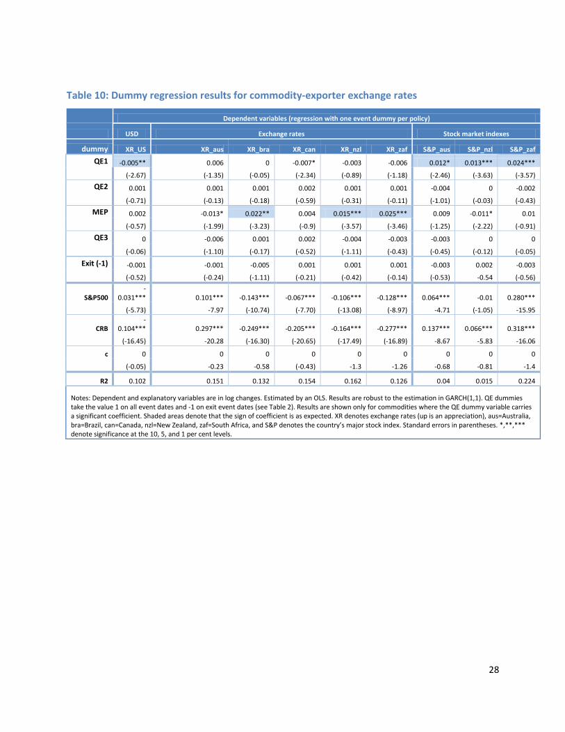
Dummy regression results of log changes in the exchange rates of commodity exporters on separate dummies for LSAP1, LSAP2, and MEP, LSAP3 and the exit are shown in Table 10. Contrary to our findings in the previous section, most statistically significant responses are now as expected: most commodity currencies appreciated (when coefficients are statistically significant).21 This suggests that markets are not segmented, but that there were important spillover effects into currencies. Moreover, the results for commodity-exporter stock indexes (last three columns) showed an increase for all statistically significant responses on LSAP1 announcement days.22 Thus, while we do not find that commodity prices themselves rose in a consistent way on LSAP announcement days, investors might have instead sought exposure to commodity-related assets such as commodity-exporter currencies or stock markets in response to LSAP announcements. Again, results are robust to the specification.

The results could suggest that LSAP announcements have been taken as a signal that economic conditions were worse than previously anticipated, implying a weaker U.S. currency in the first place, mechanically leading to an appreciation of other currencies vis-à-vis the U.S. dollar. However, signaling weaker U.S. growth could also trigger a downward revision to expectations for commodity exports, partly offsetting the first effect. In addition, for commodity producers, lower U.S. interest rates would lead to stronger commodity prices and an appreciation of commodity currencies. Alternatively, results could imply that portfolio reallocation effects

21 In contrast, when estimating the impact on the currencies of major advanced countries that do not primarily export commodity products (Japan, United Kingdom, Switzerland, euro area), we find that their currencies depreciated. 22 We also test for the impact on commodity-specific stock indexes (metals, energy), but do not find any statistically significant responses.

15

(including international reallocations) dominated the near-term positive economic effects on the U.S. economy.

5.2. Mean-return and market-return models

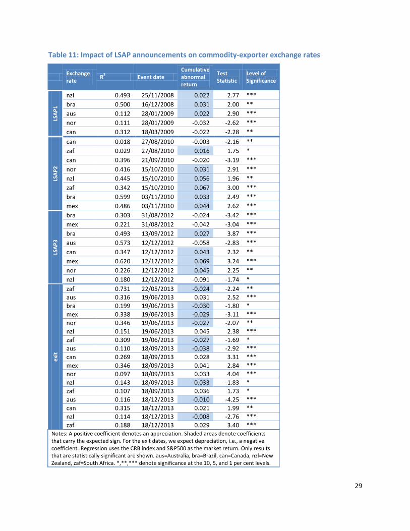
Table 11 presents the results of the event-study analysis (market-return model) estimating the impact of LSAPs on commodity-exporter exchange rates. Most statistically significant responses are again as expected and confirm our results from the dummy variable regression: commodity currencies appreciated on LSAP announcement dates. We do not find any evidence for an impact of MEP announcement dates on commodity-exporter currencies. One interpretation is that, although MEP had a similar impact on long-term yields compared with LSAPs, it did not change the amount of liquidity within the financial system and thus might not have had the same impact on other countries. Results are consistent for all three LSAP programs, however. The notable recurrent exception is the Norwegian krone, which depreciated in most statistically significant instances. This may be related to the fact that the country operates a large sovereign wealth fund that likely cushions the impact of international news such as QE announcements on the exchange rate. Abstracting from this exception, currency responses are largely as expected.23 LSAPs triggered lower U.S. interest rates, and international investors appear to have turned to commodity-exporter currencies in search of higher yields, leading to an appreciation of commodity currencies.

Last, the evidence of an impact of the exit on commodity-exporter exchange rates is less clear (with some currencies appreciating, while others depreciated). As noted above, this might be related to the fact that commodity-exporter exchange rates reacted in a similar fashion to exit announcements as the explanatory variables, i.e., the S&P and the CRB index. In this case, the abnormal return, i.e., the movement of commodity-exporter exchange rates beyond their correlation with S&P500 and the U.S. nominal effective exchange rate, is not statistically significant, which is to say that exchange rates did not react any more strongly than usual correlation with other variables would suggest. Also, the overall smaller effect of exit announcements on commodity-exporter exchange rates may relate to factors outside the analysis. In particular, while emerging markets were growing strongly over the 2008-2011 period (“decoupling”), portfolio reallocation effects may have initially been directed more toward emerging markets, and thus also toward countries exporting commodities to these markets. By 2013, however, emerging markets were no longer expected to continue to strongly outperform developed world markets. The effects of QE exit announcements may thus have

23 Similarly, the response of the Canadian dollar is sometimes opposite to other commodity-exporter currencies. If LSAP announcements were interpreted as a signal that U.S. economic conditions were worse than previously anticipated, this could possibly have also been interpreted as a signal for weaker economic growth in Canada, which is closely tied to the U.S. economy, and thus a weaker Canadian currency.

16

been dissipated across a broader set of countries. Alternatively, the news may have been of “smaller magnitude” relative to the earlier LSAP announcements.

Turning to commodity-exporter stock indexes, whether broad or commodity-specific, we find that the latter increased (Table 12) on LSAP announcement dates (again with the exception of Norwegian and Canadian stock markets, where results are less clear). This confirms our previous results that there were important spillover effects into commodity-exporter stock markets. Cumulative abnormal returns are also statistically significant in subsequent LSAP rounds, even for the MEP, and carry the predicted sign in most cases. Moreover, we observe the opposite effect for exit announcements, i.e., a fall in commodity-exporter stock indexes in almost all cases. As the tone of U.S. monetary policy turned to the tapering of asset purchases, U.S. bond yields increased. This likely attracted international investors, who might have sold commodity-exporter stock assets to increase their U.S. exposure. As a result, stock indexes in commodity-producing countries fell. Thus, while there is little evidence of a direct impact of exit announcements on commodity prices, commodity-exporter countries were indeed affected indirectly via the reaction of their stock markets.

6. LSAP vs. non-LSAP and macroeconomic surprises Another means to analyze whether LSAPs had an impact on commodity prices is to compare the response of macroeconomic surprises pre- and post-LSAP. Under normal economic circumstances, it has been shown that positive macroeconomic surprises lead to increases in some commodity prices, albeit much less than with financial assets.24 This should also be true in the case of macro surprises in an LSAP environment, but with one notable difference: in normal times, a positive macro surprise might also result in a change in the expectations for the future path of monetary policy (i.e., positive surprises should lead to a tightening). Thus, the effect on commodity prices might be partially offset by the expected increase in interest rates. But in the context of LSAPs conducted at the effective lower bound, a positive macro surprise may not translate immediately into an expected increase in interest rates (or a change in a previously announced plan of asset purchases). Thus, in principle, commodity prices could be more responsive to positive macro surprises in an environment of LSAPs.25

To test this hypothesis, we use a GARCH(1, 1) model to estimate the effect of macro surprises on oil prices prior to, and since, the introduction of LSAPs. The methodology resembles the approach in the first event study: the log change in oil prices is simply regressed on a surprise variable over two different sample periods (pre-LSAP: 2005 to October 2008; post-LSAP: December 2008 to March 2011). Surprise variables take the value 0 whenever there was no 24 See, for instance, Roache and Rossi (2009). 25 In this way, just as fiscal policy may be “supercharged” at the effective lower bound, so would the effect on commodity prices.

17

announcement, and the scaled magnitude of the surprise, computed as the z-score (i.e., the actual value announced minus the expected value, divided by the standard deviation of the surprises), on announcement dates.26 Independent variables include the surprise variables and their lags, as well as the change in the log U.S. nominal effective exchange rate. A set of 15 U.S. macroeconomic surprises are considered, including FOMC announcements, GDP, jobless claims, non-farm payrolls, PMIs and industrial production.

Table 13 shows the regression results for a selection of macro surprises. Overall, we find that oil prices appear to have become more sensitive to macroeconomic surprises during the period of LSAPs, consistent with our priors. In particular, there is a statistically significant response of the change in oil prices to the surprise in the announcement of eight macroeconomic variables during LSAP periods, whereas there is little evidence of a response of oil prices pre-LSAP.27 Most positive macroeconomic surprises are associated with an increase in oil prices: in six out of eight cases, the log oil price change increases following a positive macroeconomic surprise. In addition, a dummy variable that regroups all surprise dummy variables is now statistically significant and carries a positive coefficient. This suggests that oil prices have become more sensitive to macroeconomic surprises in LSAP periods and tend to increase with positive surprises.

Commodity prices and fundamentals

The results give some support to the view that LSAPs by the Fed did not have a significant impact on commodity prices. This suggests that other factors were the primary drivers behind the increase in commodity prices that started in mid-2010, including:

• Strong ongoing demand from EMEs across most commodity groups. For example, while there was a slowdown in advanced-economy oil demand, EME demand (and Chinese demand in particular) remained robust (Charts 4 and 5).

• Supply constraints meant that supply responses were limited—long lag times in bringing new reserves on stream and unfavourable weather (for agricultural commodities) did not allow the supply of commodities to respond swiftly to counter the increase in prices.

• Stocks of crude oil and agricultural products have generally been falling since the summer of 2010 (Yellen 2011).

26 The expected value is the median Bloomberg survey. The surprise variable carries a positive sign for news that is positive in an economic sense (e.g., the unemployment rate has an inverted sign). 27 The fact that we do not find a statistically significant response of oil prices to macroeconomic news is consistent with the literature. See, for instance, Roache and Rossi (2009).

18

These fundamental factors, among others, are the most likely reasons why commodity prices rose sharply after March 2009.28

7. Conclusion In this paper, we study the response of commodity prices to the Federal Reserve’s LSAPs from 2008 to 2012, as well as to the beginning of the communication of an exit policy in 2013. Our analysis does not provide evidence that LSAPs fuelled the rise in commodity prices. Using two types of event studies, we show that abnormal returns of commodity prices were typically not statistically significantly different from zero. In fact, oil prices tended to fall on announcement dates, particularly with LSAP1. The results are robust to different estimation and specification methods. The results suggest that other factors, such as supply constraints and recovering demand on the back of the global recovery, were most likely the primary drivers behind the increase in commodity prices that started in mid-2010 (Charts 4 and 5).

Nevertheless, results suggest that LSAPs did have spillover effects on commodity-producing countries, i.e., on commodity currencies and stock indexes. Indeed, commodity-exporter currencies tended to appreciate upon LSAP announcements, while commodity-exporter stock markets posted gains. Similarly, commodity-exporter stock markets fell upon tapering announcements. This suggests that while investors might not have reacted to LSAPs by directly investing into commodities, they may have increased their exposure to commodities by investing in commodity-related assets such as commodity currencies and commodity-heavy equity markets. Similarly, as the Fed started to reduce the pace of its LSAP purchases in 2013, U.S. bond yields rose and attracted foreign investors, leading to a decline in interest in commodity-exporter exchange rates and stock indexes.

Last, our results suggest that oil prices have become more sensitive to surprises in macroeconomic announcements during LSAP periods―where positive macroeconomic news tends to be associated with a rise in commodity prices when monetary policy is at the effective lower bound. This result does not, however, suggest that unconventional policy per se contributed to higher commodity prices.

Several possible extensions are left for future work. First, it would be interesting to construct a measure of the surprise element of QE announcements. Second, one caveat about event studies is that they cannot estimate the duration impact of QE announcements. Whether QE had a permanent impact on commodity-exporter stock markets and currencies is beyond the scope of our research, but would be worthwhile to address through alternative models.

28 Some observers argue that the growing financialization of commodity markets has also led to elevated prices, but the evidence is mixed, at best.

19

8. References Antoniou, A. and A.J. Foster. 1992. “The Effect of Futures Trading on Spot Price Volatility:

Evidence for Brent Crude Oil using GARCH.” Journal of Business Finance and Accounting 19(4): 473‒84.

Frankel, J.A. and A.K. Rose. 2010. “Determinants of Agricultural and Mineral Commodity Prices.” HKS Faculty Research Working Paper No. RWP10-038.

Gagnon, J., M. Raskin, J. Remache and B. Sack. 2010. "Large-Scale Asset Purchases by the Federal Reserve: Did They Work?" FRB of New York Staff Report No. 441.

Glick, R. and S. Leduc. 2012. “Central Bank Announcements of Asset Purchases and the Impact on Global Financial and Commodity Markets.” Journal of International Money and Finance 31(8): 2078‒101.

Kozicki, S., E. Santor and L. Suchanek. 2011. “Unconventional Monetary Policy: The International Experience with Central Bank Asset Purchases.” Bank of Canada Review (Spring 2011): 13–25.

McKenzie, A.M., M.R. Thomsen and B. Dixon. 2004. “The performance of event study approaches using daily commodity futures returns.” Journal of Futures Markets, vol. 24, no. 6, pp. 533–55.

Murray, J. 2011. “Commodity Prices: The Long and the Short of It.” Remarks at the IPAC-Saskatchewan/Johnson/Shoyama Graduate School of Public Policy, 10 February.

Neely, C.J. 2010. “The Large-Scale Asset Purchases Had Large International Effects.” Federal Reserve Bank of St. Louis Working Paper No. 2010-018, July.

Payne, R. 2003. “Informed Trade in Spot Foreign Exchange Markets: An Empirical Investigation.” Journal of International Economics, vol. 61, issue 2, pp. 307─28.

Ramsey, J. B. (1969). "Tests for Specification Errors in Classical Linear Least Squares Regression Analysis". Journal of the Royal Statistical Society Series B, vol. 31, issue 2, pp. 350–371.

Reinhart, V. 2011. “Hearing on How Federal Reserve Policies Add to Hard Times at the Pump.” Statement before the United States House of Representatives, 25 May.

Roache S.K. and M. Rossi. 2009. “The Effects of Economic News on Commodity Prices: Is Gold Just Another Commodity?” International Monetary Fund Working Paper No. 09/140.

Santor, E. and L. Suchanek. 2013. “Unconventional Monetary Policies: Evolving Practices, Their Effects and Potential Costs.” Bank of Canada Review (Spring 2013): 1‒15.

20

Swanson, E.T. 2011. “Let’s Twist Again: A High-Frequency Event-Study Analysis of Operation Twist and Its Implications for QE2.” Federal Reserve Bank of San Francisco Working Paper No. 2011-08.

Yang, J., R. B. Balyeat and D. J. Leatham. 2005. “Futures Trading Activity and Commodity Cash Price Volatility.” Journal of Business Finance & Accounting 32(1-2): 297‒323.

Yellen, J. 2011. “Commodity Prices, the Economic Outlook, and Monetary Policy.” Speech at the Economic Club of New York, New York, 11 April.

21

Appendix

A.1. Tables Table 1: Commodities included in the event study

Commodity subgroup Commodity Units Mean Standard Deviation

Energy Crude oil (WTI) USD/bbl 81 24

Natural gas USD/MMBtu 6 2 Coal USD/T 68 25 Metals Gold USD/t oz 1049 146 Silver USD/t oz 18 2

Nickel USD/MT 19727 11154 Copper USD/lb 307 73

Aluminum USD/MT 2169 540 Zinc USD/MT 1935 795 Forestry Pulp USD/MT 2024 683

Lumber USD/1000 board feet 81 24

Agriculture Live cattle USD/lb 92 6 Hogs USD/lb 68 8

Wheat USD/bushel 646 181 Canola CAD/MT 480 91

Barley CAD/MT 175 35 Corn USD/bushel 179 24

Explanatory variables CRB commodity index index 300 66

S&P 500 index 1116 177 XR index 87 4 Notes: USD denotes U.S. dollars, bbl denotes barrel, MMBtu stands for one million British Thermal Units, T stands for tons, oz for ounces, MT for metric tons, lb for pounds, and XR for U.S. nominal effective exchange rate.

22

Table 2: Announcements associated with the LSAP programs

Announcements related to LSAP1

Date Event Announcement

11/25/2008 Initial LSAP announcement Fed announces purchases of $100 billion in GSE debt and up to $500 billion in MBS.

12/01/2008 Bernanke Speech Chairman Bernanke mentions that the Fed could purchase long-term Treasuries. 12/16/2008 FOMC Statement FOMC statement first mentions possible purchase of long-term Treasuries.

1/28/2009 FOMC Statement FOMC statement says that it is ready to expand agency debt and MBS purchases, as well as to purchase long-term Treasuries.

3/18/2009 FOMC Statement FOMC will purchase an additional $750 billion in agency MBS, increase its purchases of agency debt by $100 billion, and purchase $300 billion in long-term Treasuries.

Announcements related to LSAP2

Date Event Announcement

08/10/2010 FOMC Statement

The Fed will keep constant its holdings of securities at their current level by reinvesting principal payments from agency debt and agency MBS in longer-term Treasury securities.

08/27/2010 Bernanke Speech at Jackson Hole

Bernanke describes "conducting additional purchases of longer-term securities" as a tool, and "is prepared to provide additional monetary accommodation through unconventional measures ...."

09/21/2010 FOMC Statement "The Committee [...] is prepared to provide additional accommodation if needed."

10/12/2010 Minutes release

"Several members noted that unless the pace of economic recovery strengthened or underlying inflation moved back toward a level consistent with the Committee’s mandate, they would consider it appropriate to take action soon."

10/15/2010 Bernanke Speech in Boston

"Given the Committee's objectives, there would appear―all else being equal―to be a case for further action."

11/03/2010 FOMC Statement (LSAP2)

The Fed announces the purchase of a further $600 billion of longer-term Treasury securities by the end of 2011Q2, a pace of about $75 billion per month.

Announcements related to MEP

Date Event Announcement 08/09/2011 FOMC Statement The Fed will keep low levels for the federal funds rate at least through mid-2013.

09/21/2011 FOMC Statement

The Fed announces the Maturity Extension Program (purchase of $400 billion of Treasury securities with remaining maturities of 6 years to 30 years and sale of an equal amount of Treasury securities with remaining maturities of 3 years or less) and the reinvestment of principal payments from its holdings of agency debt and agency MBS in agency MBS.

Announcements related to LSAP3

Date Event Announcement

31/8/2012 Jackson Hole Speech

Bernanke states that “the stagnation of the labor market in particular is a grave concern…” and the Fed “…will provide additional policy accommodation as needed” – which the market interprets as increasing odds of further QE.

13/09/2012 FOMC Statement The Fed announces purchases of $40 billion of agency mortgage-backed securities per month until the labor market improves "substantially."

12/12/2012 FOMC Statement The Fed announces it will purchase longer-term Treasury securities after MEP is completed at the end of the year, initially at a pace of $45 billion per month.

23

Table 2 (continued): Announcements associated with the LSAP programs

Announcements related to the exit

Date Event Announcement

22/05/2013 Testimony to Congress The Fed will cut back on bond purchases some time in “the next few meetings.”

19/06/2013 FOMC Statement The Fed announces that it could “moderate the monthly pace of purchases later this year.”

18/09/2013 FOMC Statement

Financial markets widely anticipated the beginning of tapering, but the FOMC did not announce it, citing concerns about the impact of higher interest rates on the economy, particularly on mortgage rates on housing.

18/12/2013 FOMC Statement The Fed announces plans to cut monthly bond purchases to $75 billion from $85 billion.

24

Table 3: Dummy regression results for commodity prices

Dependent

variable Dependent variable dummy gold dummy oil cattle gold silver corn barley

QE (all dates except exit)

0.004* QE1 -0.041* 0 -0.013 -0.025 0.007 -0.002 -2.07 (-2.24) (-0.01) (-1.07) (-1.86) (-0.29) (-0.15)

QE2 -0.004 0.001 -0.003 -0.002 -0.001 0.012*** (-0.76) (-0.33) (-0.49) (-0.20) (-0.08) (-5.24) MEP -0.02 0.003 0.016 -0.055*** 0.001 0 (-1.93) (-0.12) (-1.02) (-7.27) -0.02 0 QE3 0.012 0.009*** 0.016** 0.036** -0.005 0 (-0.57) (-4.69) (-3.18) (-2.96) (-0.28) 0 Exit (-1) 0.007 0.002 -0.001 -0.013 -0.003 0 -0.8 -0.27 (-0.06) (-1.11) (-0.21) 0

xr -0.963*** xr -0.744*** 0.01 -0.968*** -1.385*** -0.438*** -0.059 (-30.71) (-11.34) -0.32 (-32.81) (-26.18) (-7.79) (-0.95)

S&P500 -0.061*** S&P500 0.320*** 0.075*** -0.058*** 0.027 0.080*** -0.011 (-5.09) -14.1 -5.96 (-4.80) -1.48 -3.87 (-0.70) c 0.000* c 0.001* 0 0.000* 0 0 0.080*** -2.36 -2.56 -0.36 -2.32 -0.63 -0.89 -4.43

ARCH ARCH L.arch 0.068*** L.arch 0.092*** 0.103*** 0.077*** 0.106*** 0.143*** -2.22

-11.25 -13.02 -12.51 -15.37 -17.23 -12.61 0 L.garch 0.922*** L.garch 0.899*** 0.650*** 0.912*** 0.895*** 0.817*** 0.128***

-114.84 -107.09 -28.77 -137.81 -143.53 -47.16 -26 c 0.000*** c 0.000** 0.000*** 0.000*** 0.000** 0.000*** 0.866*** -3.55 -3.04 -13.34 -4.57 -2.91 -6.29 -219.76

Notes: Dependent and explanatory variables are in log changes. Estimated by a GARCH(1,1). QE dummies take the value 1 on all event dates (see Table 2). XR stands for the U.S. nominal effective exchange rate. S&P500 denotes the Standard and Poor’s 500 stock market index. ARCH stands for Autoregressive Conditional Heteroskedasticity. L.arch denotes the estimated ARCH parameter, and l.garch is the estimated Generalized AutoRegressive Conditional Heteroskedasticity (GARCH) parameter. c denotes the constant. Results are shown only for commodities where the QE dummy variable carries a significant coefficient. Shaded areas denote that the sign of the cumulative abnormal return is as expected. Standard errors are in (parentheses). *,**,*** denote significance at the 10, 5, and 1 per cent levels.

25

Table 4: LSAP1: Results from mean-return model

Commodity R2 Event date

Cumulative abnormal return

Test statistic

Level of significance

hogs 0.008 25/11/2008 0.023 3.90 *** silver 0.022 25/11/2008 0.069 1.66 *

aluminum 0.080 01/12/2008 -0.035 -2.00 ** nickel 0.199 01/12/2008 -0.022 -1.68 * coal 0.041 01/12/2008 0.066 3.62 *** canola 0.065 01/12/2008 -0.042 -1.79 * barley 0.087 01/12/2008 0.103 2.13 **

oil 0.063 16/12/2008 -0.091 -2.71 *** pulp 0.072 16/12/2008 0.009 8.57 *** gold 0.060 16/12/2008 0.031 1.87 * wheat 0.070 16/12/2008 0.087 10.26 *** coal 0.044 16/12/2008 -0.082 -4.74 *** corn 0.067 16/12/2008 0.083 2.67 ***

barley 0.033 28/01/2009 0.097 5.05 *** aluminum 0.016 18/03/2009 0.044 1.80 * Notes: Only results that are statistically significant are shown. Shaded areas denote that the sign of the cumulative abnormal return is as expected. *,**,*** denote significance at the 10, 5, and 1 per cent levels.

Table 5: LSAP1: Results from the market-return model

Commodity R2 Event date Cumulative

abnormal return Test

statistic Level of

significance hogs 0.033 25/11/2008 0.029 3.84 ***

aluminium 0.350 01/12/2008 -0.036 -2.17 ** barley 0.378 01/12/2008 0.090 1.88 * canola 0.283 01/12/2008 -0.051 -1.95 * coal 0.441 01/12/2008 0.057 3.37 ***

aluminium 0.224 16/12/2008 -0.026 -1.98 ** coal 0.328 16/12/2008 -0.117 -3.01 *** copper 0.635 16/12/2008 -0.077 -1.84 * gold 0.080 16/12/2008 0.026 2.15 ** oil 0.273 16/12/2008 -0.150 -3.03 *** pulp 0.265 16/12/2008 0.013 1.88 * wheat 0.323 16/12/2008 0.043 1.74 *

hogs 0.050 18/03/2009 -0.013 -2.25 ** pulp 0.067 18/03/2009 0.015 3.55 *** Notes: Regressions use the CRB index, the S&P500 index, and the U.S. nominal effective exchange rate as the market return, and only the latter two for commodities included in the CRB index, see text. Only results that are statistically significant are shown. Shaded areas denote that the sign of the cumulative abnormal return is as expected. *,**,*** denote significance at the 10, 5, and 1 per cent levels.

26

Table 6: LSAP2: Results from the market-return model

Commodity R2 Event date

Cumulative abnormal

return Test

statistic Level of

significance canola 0.292 10/08/2010 -0.055 -2.95 *** cattle 0.383 10/08/2010 0.014 2.69 *** coal 0.149 10/08/2010 -0.010 -2.04 ** copper 0.512 10/08/2010 0.013 1.79 * gas 0.018 10/08/2010 -0.034 -1.76 *

cattle 0.016 27/08/2010 -0.010 -2.39 *** pulp 0.121 27/08/2010 -0.001 -2.70 ***

barley 0.054 21/09/2010 -0.087 -5.33 *** coal 0.056 21/09/2010 0.019 2.12 ** gold 0.028 21/09/2010 0.010 1.77 * pulp 0.004 21/09/2010 0.003 2.16 ** wheat 0.040 21/09/2010 -0.044 -1.98 **

barley 0.373 12/10/2010 -0.131 -3.00 *** lumber 0.080 12/10/2010 0.049 2.29 ** nickel 0.489 12/10/2010 -0.017 -1.70 * pulp 0.051 12/10/2010 0.002 2.20 ** silver 0.256 12/10/2010 0.024 2.10 **

corn 0.063 15/10/2010 -0.031 -4.98 *** nickel 0.220 15/10/2010 -0.013 -1.85 * pulp 0.002 15/10/2010 0.003 4.24 *** wheat 0.002 15/10/2010 -0.036 -2.60 ***

barley 0.141 03/11/2010 0.022 2.65 *** canola 0.088 03/11/2010 0.035 1.98 ** cattle 0.007 03/11/2010 -0.009 -2.69 *** coal 0.205 03/11/2010 0.009 2.11 ** oil 0.067 03/11/2010 0.030 3.72 *** pulp 0.041 03/11/2010 -0.004 -3.22 *** Notes: Regressions use the CRB index, the S&P500 index, and the U.S. nominal effective exchange rate as the market return, and only the latter two for commodities included in the CRB index. Only results that are statistically significant are shown. Shaded areas denote that the sign of the cumulative abnormal return is as expected. *,**,*** denote significance at the 10, 5, and 1 per cent levels.

27

Table 7: MEP: Results from the market-return model

Commodity R2 Event date Cumulative abnormal return

Test Statistic

Level of Significance

gas 0.186 30/08/2011 0.030 2.20 ** lumber 0.073 30/08/2011 0.030 2.14 ** aluminum 0.263 30/08/2011 0.010 1.77 * pulp 0.028 21/09/2011 0.020 2.91 *** nickel 0.107 21/09/2011 -0.050 -2.22 ** hogs 0.004 30/08/2011 -0.010 -2.64 *** wheat 0.081 21/09/2011 -0.020 -1.75 * coal 0.193 09/08/2011 0.010 1.65 * barley 0.004 21/09/2011 0.000 -6.44 *** corn 0.045 21/09/2011 -0.040 -2.23 ** Notes: Regression uses the CRB index, the S&P500 index, and the U.S. nominal effective exchange rate as the market return, and only the latter two for commodities included in the CRB index. Only results that are statistically significant are shown. Shaded areas denote that the sign of the cumulative abnormal return is as expected. *,**,*** denote significance at the 10, 5, and 1 per cent levels.

Table 8: LSAP3: Results from the market-return model

Commodity R2 Event date Cumulative abnormal return

Test Statistic

Level of Significance

oil 0.500 13/09/2012 -3.508 -1.79 * gas 0.048 12/12/2012 -0.329 -5.82 *** hogs 0.052 12/12/2012 -1.253 -6.82 *** Notes: Regression uses the CRB index, the S&P500 index, and the U.S. nominal effective exchange rate as the market return, and only the latter two for commodities included in the CRB index. Only results that are statistically significant are shown. Shaded areas denote that the sign of the cumulative abnormal return is as expected. *,**,*** denote significance at the 10, 5, and 1 per cent levels.

Table 9: Exit: Results from the market-return model

Commodity R2 Event date

Cumulative abnormal return Test statistic

Level of significance

coal 0.025 2013/05/22 -0.070 -3.04 *** zinc 0.413 2013/05/22 0.083 1.91 * barley 0.226 2013/05/22 -0.023 -2.06 ** nickel 0.086 2013/06/19 0.076 2.90 *** wheat 0.332 2013/06/19 0.029 1.73 * silver 0.046 2013/06/19 -0.069 -4.26 *** oil 0.563 2013/12/18 0.026 2.73 *** brent 0.618 2013/12/18 0.037 3.05 *** canola 0.249 2013/12/18 -0.041 -2.05 ** Notes: The sign of the dummy variable is -1, i.e., the shaded coefficients (positive) indicate that the price decreased, as expected. The regression uses the CRB index, the S&P500 index, and the U.S. nominal effective exchange rate as the market return, and only the latter two for commodities included in the CRB index. Only results that are statistically significant are shown. *,**,*** denote significance at the 10, 5, and 1 per cent levels.

28

Table 10: Dummy regression results for commodity-exporter exchange rates

Dependent variables (regression with one event dummy per policy)

USD Exchange rates Stock market indexes

dummy XR_US XR_aus XR_bra XR_can XR_nzl XR_zaf S&P_aus S&P_nzl S&P_zaf

QE1 -0.005** 0.006 0 -0.007* -0.003 -0.006 0.012* 0.013*** 0.024*** (-2.67) (-1.35) (-0.05) (-2.34) (-0.89) (-1.18) (-2.46) (-3.63) (-3.57)

QE2 0.001 0.001 0.001 0.002 0.001 0.001 -0.004 0 -0.002 (-0.71) (-0.13) (-0.18) (-0.59) (-0.31) (-0.11) (-1.01) (-0.03) (-0.43)

MEP 0.002 -0.013* 0.022** 0.004 0.015*** 0.025*** 0.009 -0.011* 0.01 (-0.57) (-1.99) (-3.23) (-0.9) (-3.57) (-3.46) (-1.25) (-2.22) (-0.91)

QE3 0 -0.006 0.001 0.002 -0.004 -0.003 -0.003 0 0 (-0.06) (-1.10) (-0.17) (-0.52) (-1.11) (-0.43) (-0.45) (-0.12) (-0.05)

Exit (-1) -0.001 -0.001 -0.005 0.001 0.001 0.001 -0.003 0.002 -0.003

(-0.52) (-0.24) (-1.11) (-0.21) (-0.42) (-0.14) (-0.53) -0.54 (-0.56)

S&P500 -

0.031*** 0.101*** -0.143*** -0.067*** -0.106*** -0.128*** 0.064*** -0.01 0.280***

(-5.73) -7.97 (-10.74) (-7.70) (-13.08) (-8.97) -4.71 (-1.05) -15.95

CRB -

0.104*** 0.297*** -0.249*** -0.205*** -0.164*** -0.277*** 0.137*** 0.066*** 0.318***

(-16.45) -20.28 (-16.30) (-20.65) (-17.49) (-16.89) -8.67 -5.83 -16.06

c 0 0 0 0 0 0 0 0 0

(-0.05) -0.23 -0.58 (-0.43) -1.3 -1.26 -0.68 -0.81 -1.4

R2 0.102 0.151 0.132 0.154 0.162 0.126 0.04 0.015 0.224

Notes: Dependent and explanatory variables are in log changes. Estimated by an OLS. Results are robust to the estimation in GARCH(1,1). QE dummies take the value 1 on all event dates and -1 on exit event dates (see Table 2). Results are shown only for commodities where the QE dummy variable carries a significant coefficient. Shaded areas denote that the sign of coefficient is as expected. XR denotes exchange rates (up is an appreciation), aus=Australia, bra=Brazil, can=Canada, nzl=New Zealand, zaf=South Africa, and S&P denotes the country’s major stock index. Standard errors in parentheses. *,**,*** denote significance at the 10, 5, and 1 per cent levels.

29

Table 11: Impact of LSAP announcements on commodity-exporter exchange rates

Exchange rate R2 Event date

Cumulative abnormal return

Test Statistic

Level of Significance

LSAP

1

nzl 0.493 25/11/2008 0.022 2.77 *** bra 0.500 16/12/2008 0.031 2.00 ** aus 0.112 28/01/2009 0.022 2.90 *** nor 0.111 28/01/2009 -0.032 -2.62 *** can 0.312 18/03/2009 -0.022 -2.28 **

LSAP

2

can 0.018 27/08/2010 -0.003 -2.16 ** zaf 0.029 27/08/2010 0.016 1.75 * can 0.396 21/09/2010 -0.020 -3.19 *** nor 0.416 15/10/2010 0.031 2.91 *** nzl 0.445 15/10/2010 0.056 1.96 ** zaf 0.342 15/10/2010 0.067 3.00 *** bra 0.599 03/11/2010 0.033 2.49 *** mex 0.486 03/11/2010 0.044 2.62 ***

LSAP

3

bra 0.303 31/08/2012 -0.024 -3.42 *** mex 0.221 31/08/2012 -0.042 -3.04 *** bra 0.493 13/09/2012 0.027 3.87 *** aus 0.573 12/12/2012 -0.058 -2.83 *** can 0.347 12/12/2012 0.043 2.32 ** mex 0.620 12/12/2012 0.069 3.24 *** nor 0.226 12/12/2012 0.045 2.25 ** nzl 0.180 12/12/2012 -0.091 -1.74 *

exit

zaf 0.731 22/05/2013 -0.024 -2.24 ** aus 0.316 19/06/2013 0.031 2.52 *** bra 0.199 19/06/2013 -0.030 -1.80 * mex 0.338 19/06/2013 -0.029 -3.11 *** nor 0.346 19/06/2013 -0.027 -2.07 ** nzl 0.151 19/06/2013 0.045 2.38 *** zaf 0.309 19/06/2013 -0.027 -1.69 * aus 0.110 18/09/2013 -0.038 -2.92 *** can 0.269 18/09/2013 0.028 3.31 *** mex 0.346 18/09/2013 0.041 2.84 *** nor 0.097 18/09/2013 0.033 4.04 *** nzl 0.143 18/09/2013 -0.033 -1.83 * zaf 0.107 18/09/2013 0.036 1.73 * aus 0.116 18/12/2013 -0.010 -4.25 *** can 0.315 18/12/2013 0.021 1.99 ** nzl 0.114 18/12/2013 -0.008 -2.76 *** zaf 0.188 18/12/2013 0.029 3.40 ***

Notes: A positive coefficient denotes an appreciation. Shaded areas denote coefficients that carry the expected sign. For the exit dates, we expect depreciation, i.e., a negative coefficient. Regression uses the CRB index and S&P500 as the market return. Only results that are statistically significant are shown. aus=Australia, bra=Brazil, can=Canada, nzl=New Zealand, zaf=South Africa. *,**,*** denote significance at the 10, 5, and 1 per cent levels.

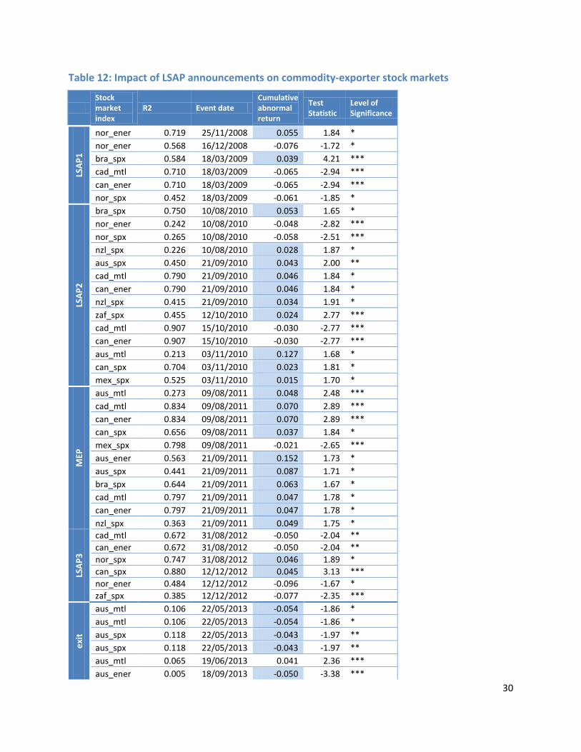
30

Table 12: Impact of LSAP announcements on commodity-exporter stock markets

Stock market index

R2 Event date Cumulative abnormal return

Test Statistic

Level of Significance

LSAP

1

nor_ener 0.719 25/11/2008 0.055 1.84 * nor_ener 0.568 16/12/2008 -0.076 -1.72 * bra_spx 0.584 18/03/2009 0.039 4.21 *** cad_mtl 0.710 18/03/2009 -0.065 -2.94 *** can_ener 0.710 18/03/2009 -0.065 -2.94 *** nor_spx 0.452 18/03/2009 -0.061 -1.85 *

LSAP

2

bra_spx 0.750 10/08/2010 0.053 1.65 * nor_ener 0.242 10/08/2010 -0.048 -2.82 *** nor_spx 0.265 10/08/2010 -0.058 -2.51 *** nzl_spx 0.226 10/08/2010 0.028 1.87 * aus_spx 0.450 21/09/2010 0.043 2.00 ** cad_mtl 0.790 21/09/2010 0.046 1.84 * can_ener 0.790 21/09/2010 0.046 1.84 * nzl_spx 0.415 21/09/2010 0.034 1.91 * zaf_spx 0.455 12/10/2010 0.024 2.77 *** cad_mtl 0.907 15/10/2010 -0.030 -2.77 *** can_ener 0.907 15/10/2010 -0.030 -2.77 *** aus_mtl 0.213 03/11/2010 0.127 1.68 * can_spx 0.704 03/11/2010 0.023 1.81 * mex_spx 0.525 03/11/2010 0.015 1.70 *

MEP

aus_mtl 0.273 09/08/2011 0.048 2.48 *** cad_mtl 0.834 09/08/2011 0.070 2.89 *** can_ener 0.834 09/08/2011 0.070 2.89 *** can_spx 0.656 09/08/2011 0.037 1.84 * mex_spx 0.798 09/08/2011 -0.021 -2.65 *** aus_ener 0.563 21/09/2011 0.152 1.73 * aus_spx 0.441 21/09/2011 0.087 1.71 * bra_spx 0.644 21/09/2011 0.063 1.67 * cad_mtl 0.797 21/09/2011 0.047 1.78 * can_ener 0.797 21/09/2011 0.047 1.78 * nzl_spx 0.363 21/09/2011 0.049 1.75 *

LSAP

3

cad_mtl 0.672 31/08/2012 -0.050 -2.04 ** can_ener 0.672 31/08/2012 -0.050 -2.04 ** nor_spx 0.747 31/08/2012 0.046 1.89 * can_spx 0.880 12/12/2012 0.045 3.13 *** nor_ener 0.484 12/12/2012 -0.096 -1.67 * zaf_spx 0.385 12/12/2012 -0.077 -2.35 ***

exit

aus_mtl 0.106 22/05/2013 -0.054 -1.86 * aus_mtl 0.106 22/05/2013 -0.054 -1.86 * aus_spx 0.118 22/05/2013 -0.043 -1.97 ** aus_spx 0.118 22/05/2013 -0.043 -1.97 ** aus_mtl 0.065 19/06/2013 0.041 2.36 *** aus_ener 0.005 18/09/2013 -0.050 -3.38 ***

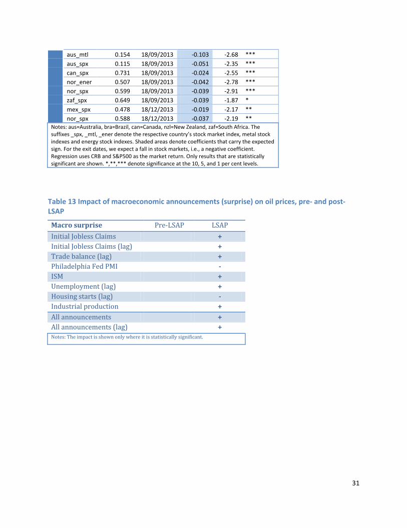
31

aus_mtl 0.154 18/09/2013 -0.103 -2.68 *** aus_spx 0.115 18/09/2013 -0.051 -2.35 *** can_spx 0.731 18/09/2013 -0.024 -2.55 *** nor_ener 0.507 18/09/2013 -0.042 -2.78 *** nor_spx 0.599 18/09/2013 -0.039 -2.91 *** zaf_spx 0.649 18/09/2013 -0.039 -1.87 * mex_spx 0.478 18/12/2013 -0.019 -2.17 ** nor_spx 0.588 18/12/2013 -0.037 -2.19 **

Notes: aus=Australia, bra=Brazil, can=Canada, nzl=New Zealand, zaf=South Africa. The suffixes _spx, _mtl, _ener denote the respective country’s stock market index, metal stock indexes and energy stock indexes. Shaded areas denote coefficients that carry the expected sign. For the exit dates, we expect a fall in stock markets, i.e., a negative coefficient. Regression uses CRB and S&P500 as the market return. Only results that are statistically significant are shown. *,**,*** denote significance at the 10, 5, and 1 per cent levels.

Table 13 Impact of macroeconomic announcements (surprise) on oil prices, pre- and post- LSAP

Macro surprise Pre-LSAP LSAP Initial Jobless Claims + Initial Jobless Claims (lag) + Trade balance (lag) + Philadelphia Fed PMI - ISM + Unemployment (lag) + Housing starts (lag) - Industrial production

+

All announcements + All announcements (lag) + Notes: The impact is shown only where it is statistically significant.

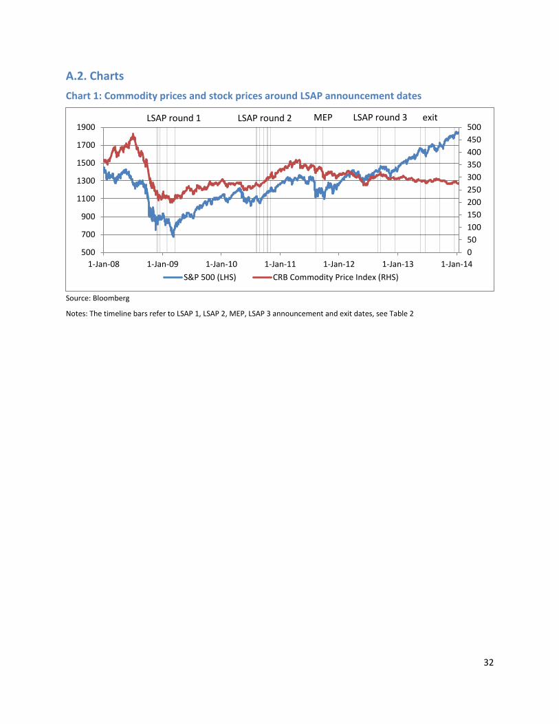
32

A.2. Charts Chart 1: Commodity prices and stock prices around LSAP announcement dates

Source: Bloomberg

Notes: The timeline bars refer to LSAP 1, LSAP 2, MEP, LSAP 3 announcement and exit dates, see Table 2

050100150200250300350400450500

500

700

900

1100

1300

1500

1700

1900

1-Jan-08 1-Jan-09 1-Jan-10 1-Jan-11 1-Jan-12 1-Jan-13 1-Jan-14S&P 500 (LHS) CRB Commodity Price Index (RHS)

LSAP round 1 LSAP round 2 LSAP round 3 exit MEP

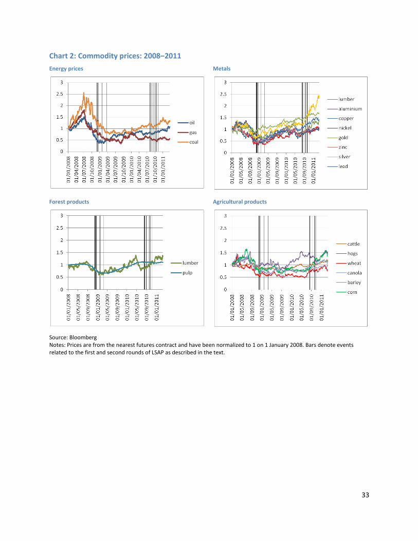
33

Chart 2: Commodity prices: 2008‒2011 Energy prices

Metals

Forest products

Agricultural products

Source: Bloomberg Notes: Prices are from the nearest futures contract and have been normalized to 1 on 1 January 2008. Bars denote events related to the first and second rounds of LSAP as described in the text.

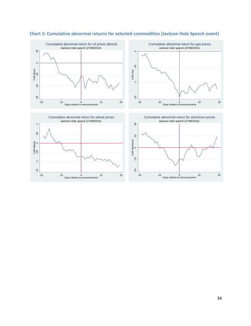
34

Chart 3: Cumulative abnormal returns for selected commodities (Jackson Hole Speech event)

-.06

-.04

-.02

0.0

2C

AR

Bre

nt

-20 -10 0 10 20Days relative to announcement

Jackson Hole speech (27/08/2010)Cumulative abnormal return for oil prices (Brent)

-.15

-.1-.0

50

CA

R G

as

-20 -10 0 10 20Days relative to announcement

Jackson Hole speech (27/08/2010)Cumulative abnormal return for gas prices

-.15

-.1-.0

50

.05

.1C

AR

Whe

at

-20 -10 0 10 20Days relative to announcement

Jackson Hole speech (27/08/2010)Cumulative abnormal return for wheat prices

-.04

-.02

0.0

2.0

4C

AR

Alu

min

um

-20 -10 0 10 20Days relative to announcement

Jackson Hole speech (27/08/2010)Cumulative abnormal return for aluminum prices

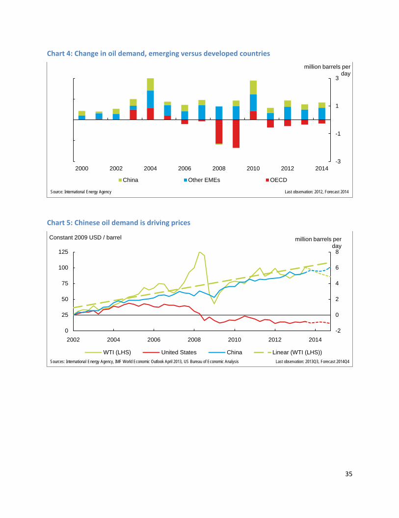
35

Chart 4: Change in oil demand, emerging versus developed countries

Chart 5: Chinese oil demand is driving prices

2000 2002 2004 2006 2008 2010 2012 2014-3

-1

1

3

million barrels per day

China Other EMEs OECD

Last observation: 2012, Forecast 2014 Source: International Energy Agency

2002 2004 2006 2008 2010 2012 2014-2

0

2

4

6

8

0

25

50

75

100

125

million barrels per day

WTI (LHS) United States China Linear (WTI (LHS))

Constant 2009 USD / barrel

Last observation: 2013Q3, Forecast 2014Q4 Sources: International Energy Agency, IMF World Economic Outlook April 2013, US Bureau of Economic Analysis