laplace transformation of linear time-varying systems transformation.pdf · laplace transformation...

RESEARCH CENTRE FOR INTEGRATED MICROSYSTEMS - UNIVERSITY OF WINDSORRESEARCH CENTRE FOR INTEGRATED MICROSYSTEMS - UNIVERSITY OF WINDSOR

Aug. 14, 2009

Laplace Transformationof

Linear Time-Varying Systems

Shervin ErfaniResearch Centre for Integrated MicroelectronicsElectrical and Computer Engineering Department

University of WindsorWindsor, Ontario N9B 3P4, Canada


Aug. 14, 20098/24/2009 2

Outline of the Presentation

• From LTV Elements to LTV Systems• Observations on LTV Systems

– Generalized-Delay System Representation– Circularly Symmetric Functions– Bivariate Time and Bifrequency Characterization

• Two-Dimensional Laplace Transform (2DLT)– The Hankel Transformation– The Mellin Transformation

• An Illustrative Example• Conclusions• References


Aug. 14, 20098/24/2009 3

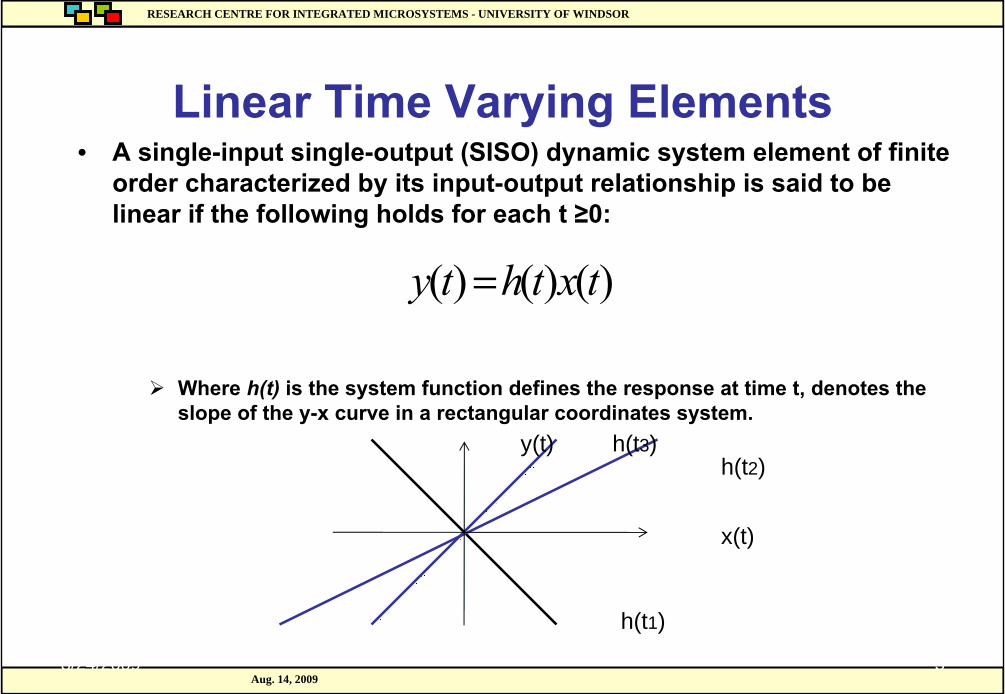
Linear Time Varying Elements

Where h(t) is the system function defines the response at time t, denotes the slope of the y-x curve in a rectangular coordinates system.

• A single-input single-output (SISO) dynamic system element of finite order characterized by its input-output relationship is said to be linear if the following holds for each t ≥0:

)()()( txthty =

h(t1)

h(t2)h(t3)

x(t)

y(t)


Aug. 14, 20098/24/2009 4

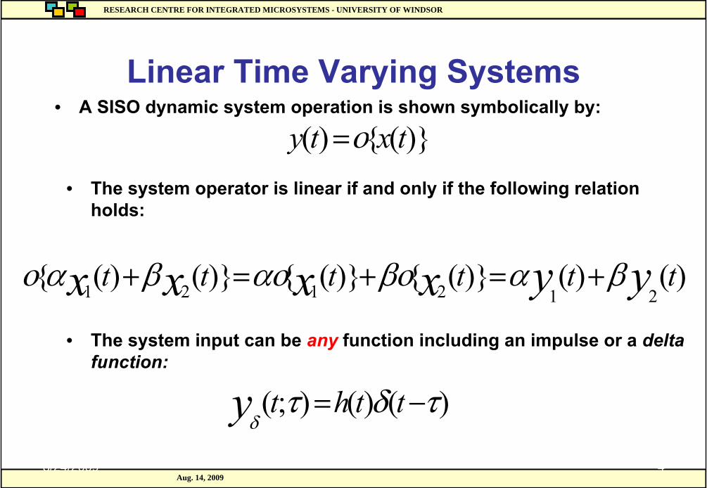
Linear Time Varying Systems• A SISO dynamic system operation is shown symbolically by:

)}({)( txty ο=• The system operator is linear if and only if the following relation

holds:

)()()}({)}({)}()({212121

tttttt yyxxxx βαβοαοβαο +=+=+

• The system input can be any function including an impulse or a delta function:

)()();( τδτδ

−= tthty


Aug. 14, 20098/24/2009 5

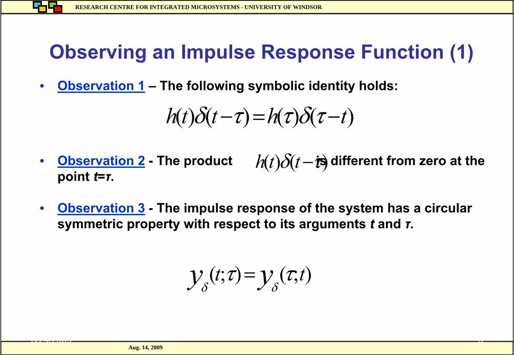
Observing an Impulse Response Function (1)• Observation 1 – The following symbolic identity holds:

)()()()( thtth −=− τδττδ

• Observation 2 - The product is different from zero at thepoint t=τ.

• Observation 3 - The impulse response of the system has a circular symmetric property with respect to its arguments t and τ.

);();( tt yy ττδδ

=

)()( τδ −tth


Aug. 14, 20098/24/2009 6

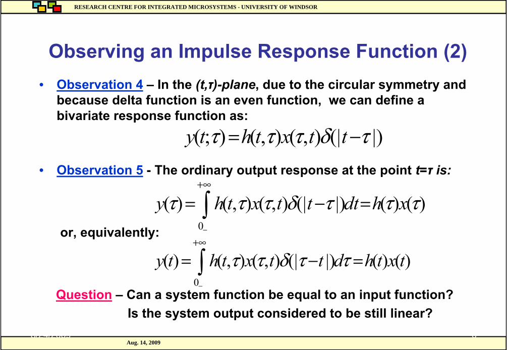
Observing an Impulse Response Function (2)• Observation 4 – In the (t,τ)-plane, due to the circular symmetry and

because delta function is an even function, we can define a bivariate response function as:

|)(|),(),();( τδτττ −= ttxthty• Observation 5 - The ordinary output response at the point t=τ is:

or, equivalently:

)()(|)(|),(),()(0

τττδτττ xhdtttxthy =−= ∫+∞

−

)()(|)(|),(),()(0

txthdttxthty =−= ∫+∞

−

ττδττ

Question – Can a system function be equal to an input function?Is the system output considered to be still linear?


Aug. 14, 20098/24/2009 7

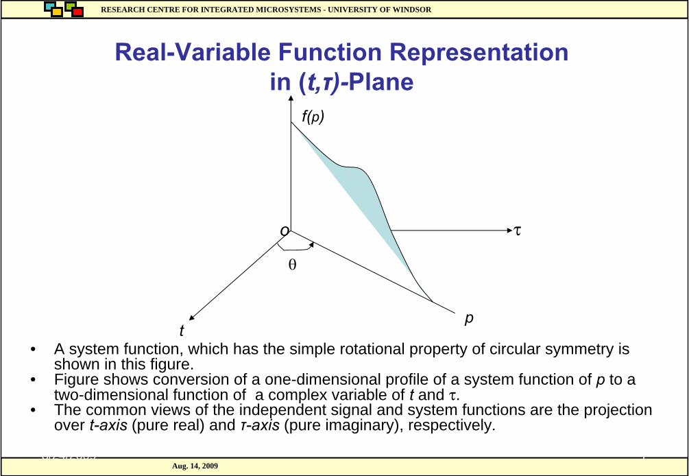
Real-Variable Function Representationin (t,τ)-Plane

• A system function, which has the simple rotational property of circular symmetry is shown in this figure.

• Figure shows conversion of a one-dimensional profile of a system function of p to a two-dimensional function of a complex variable of t and τ.

• The common views of the independent signal and system functions are the projection over t-axis (pure real) and τ-axis (pure imaginary), respectively.

t

f(p)

τ

p

o

θ


Aug. 14, 20098/24/2009 8

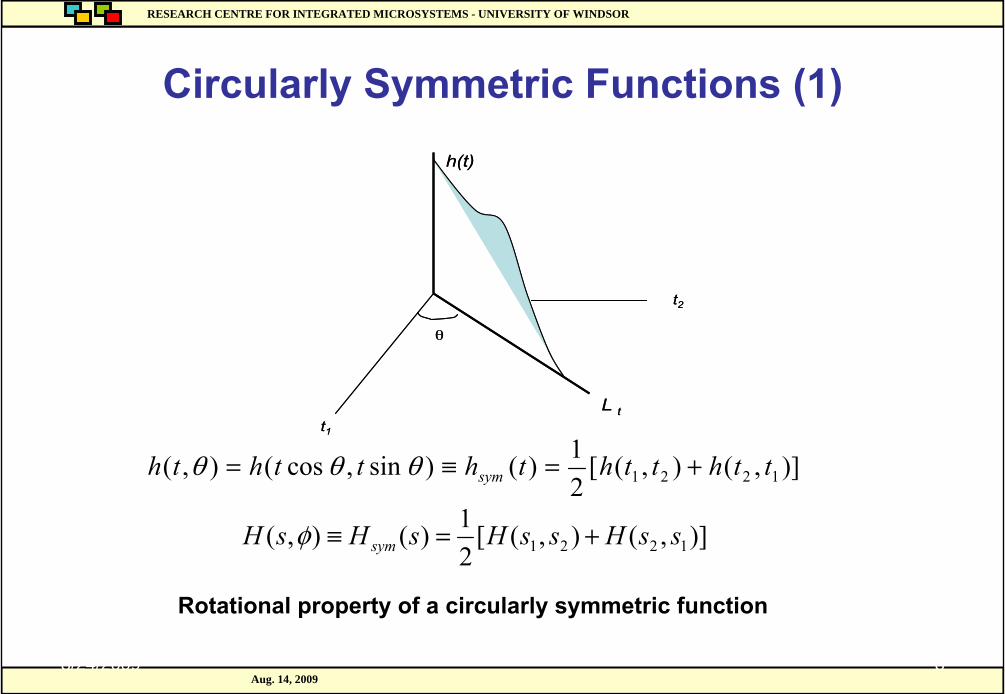
Circularly Symmetric Functions (1)

t1

h(t)

t2

L t

θ

t1

h(t)

t2

L t

θ

Rotational property of a circularly symmetric function

)],(),([21)()sin,cos(),( 1221 tthtththtthth sym +=≡= θθθ

)],(),([21)(),( 1221 ssHssHsHsH sym +=≡φ


Aug. 14, 20098/24/2009 9

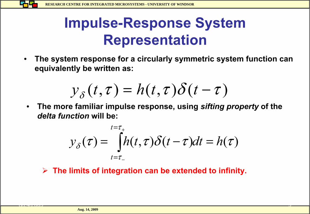
Impulse-Response System Representation

• The more familiar impulse response, using sifting property of the delta function will be:

• The system response for a circularly symmetric system function can equivalently be written as:

)()(),()( ττδτττ

τδ hdttthy

t

t

=−= ∫+

−

=

=

)(),(),( τδττδ −= tthty

The limits of integration can be extended to infinity.


Aug. 14, 20098/24/2009 10

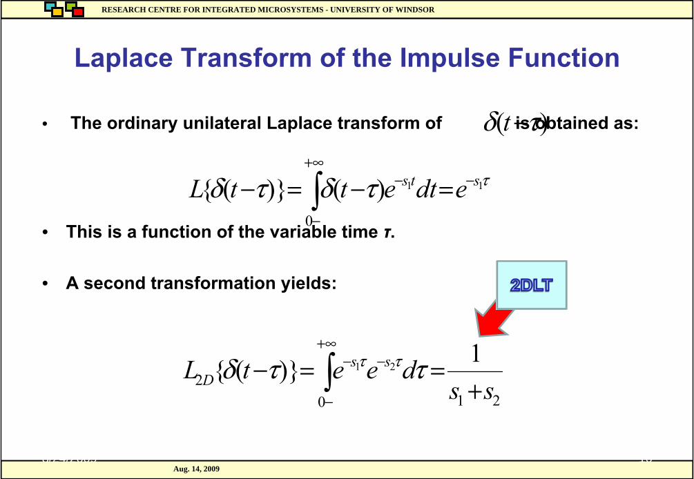
• The ordinary unilateral Laplace transform of is obtained as:

• This is a function of the variable time τ.

• A second transformation yields:

Laplace Transform of the Impulse Function

)( τδ −t

ττδτδ 11

0

)()}({ sts edtettL −+∞

−

− =−=− ∫

2102

1)}({ 21

ssdeetL ss

D +==− ∫

+∞

−

−− ττδ ττ


Aug. 14, 20098/24/2009 11

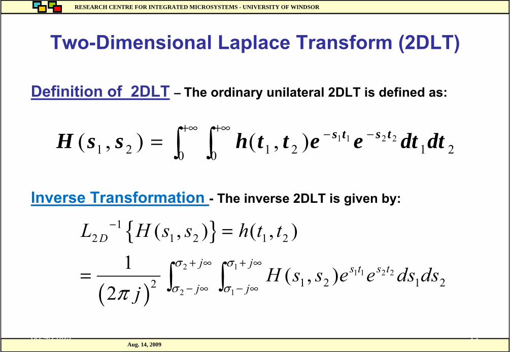
Definition of 2DLT – The ordinary unilateral 2DLT is defined as:

Inverse Transformation - The inverse 2DLT is given by:

Two-Dimensional Laplace Transform (2DLT)

20 10 21212211),(),( dtdteetthssH tsts∫ ∫

+∞ +∞ −−=

{ }

( )2 1

1 1 2 2

2 1

12 1 2 1 2

1 2 1 22

( , ) ( , )1 ( , )

2

D

j j s t s t

j j

L H s s h t t

H s s e e ds dsj

σ σ

σ σπ

−

+ ∞ + ∞

− ∞ − ∞

=

= ∫ ∫


Aug. 14, 20098/24/2009 12

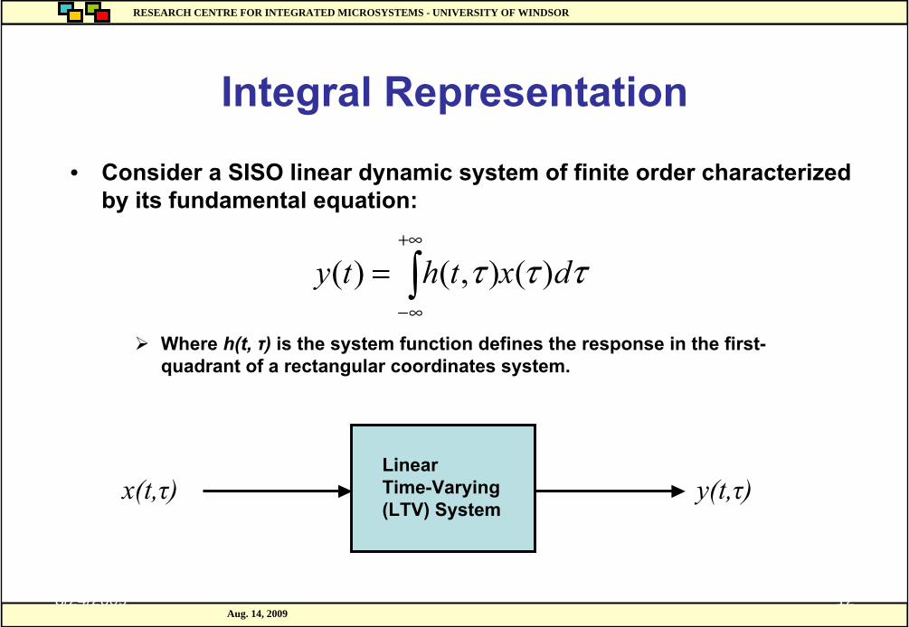
Integral Representation

Where h(t, τ) is the system function defines the response in the first-quadrant of a rectangular coordinates system.

x(t,τ) LinearTime-Varying (LTV) System

• Consider a SISO linear dynamic system of finite order characterized by its fundamental equation:

y(t,τ)

τττ dxthty )(),()( ∫+∞

∞−

=


Aug. 14, 20098/24/2009 13

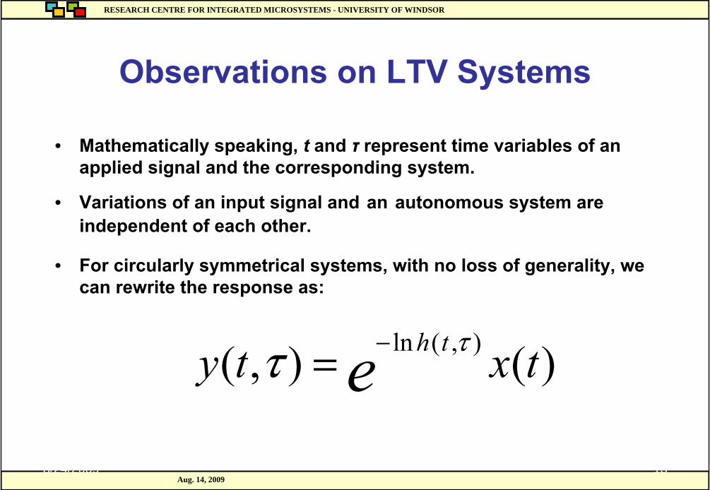
Observations on LTV Systems

• For circularly symmetrical systems, with no loss of generality, we can rewrite the response as:

• Mathematically speaking, t and τ represent time variables of an applied signal and the corresponding system.

• Variations of an input signal and an autonomous system are independent of each other.

)(),( ),(ln txty e th ττ −=


Aug. 14, 20098/24/2009 14

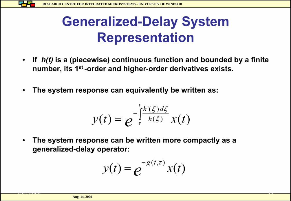
Generalized-Delay System Representation

• The system response can be written more compactly as a generalized-delay operator:

• If h(t) is a (piecewise) continuous function and bounded by a finite number, its 1st -order and higher-order derivatives exists.

• The system response can equivalently be written as:

)()( ),( txty e tg τ−=

)()( )()('

txty et

hdh

∫= −τ

ξξξ


Aug. 14, 20098/24/2009 15

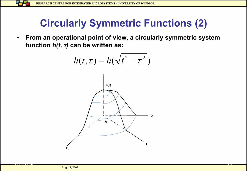
Circularly Symmetric Functions (2)• From an operational point of view, a circularly symmetric system

function h(t, τ) can be written as:

)(),( 22 ττ += thth


Aug. 14, 20098/24/2009 16

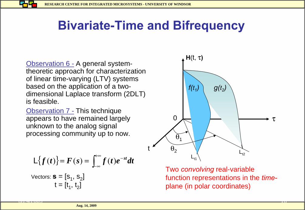
Bivariate-Time and Bifrequency

Two convolving real-variable function representations in the time-plane (in polar coordinates)

Lt1

t

τ

Lt2

f(t1) g(t2)

0

θ1

θ2

H(t, τ)

{ } ∫+∞

∞−

−== dtetfsFtf st)()()(L

Observation 6 - A general system-theoretic approach for characterization of linear time-varying (LTV) systems based on the application of a two-dimensional Laplace transform (2DLT) is feasible.Observation 7 - This technique appears to have remained largely unknown to the analog signal processing community up to now.

Vectors: s = [s1, s2]t = [t1, t2]


Aug. 14, 20098/24/2009 17

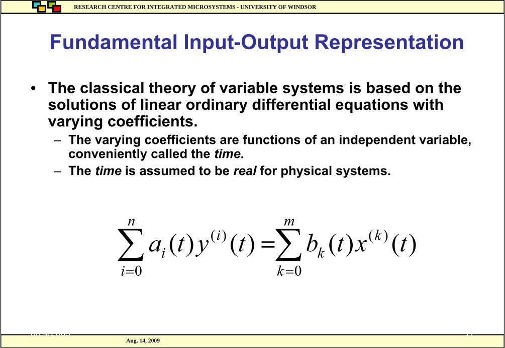
Fundamental Input-Output Representation

• The classical theory of variable systems is based on the solutions of linear ordinary differential equations with varying coefficients. – The varying coefficients are functions of an independent variable,

conveniently called the time.– The time is assumed to be real for physical systems.

∑∑==

=m

k

kk

n

i

ii txtbtyta

0

)(

0

)( )()()()(


Aug. 14, 2009

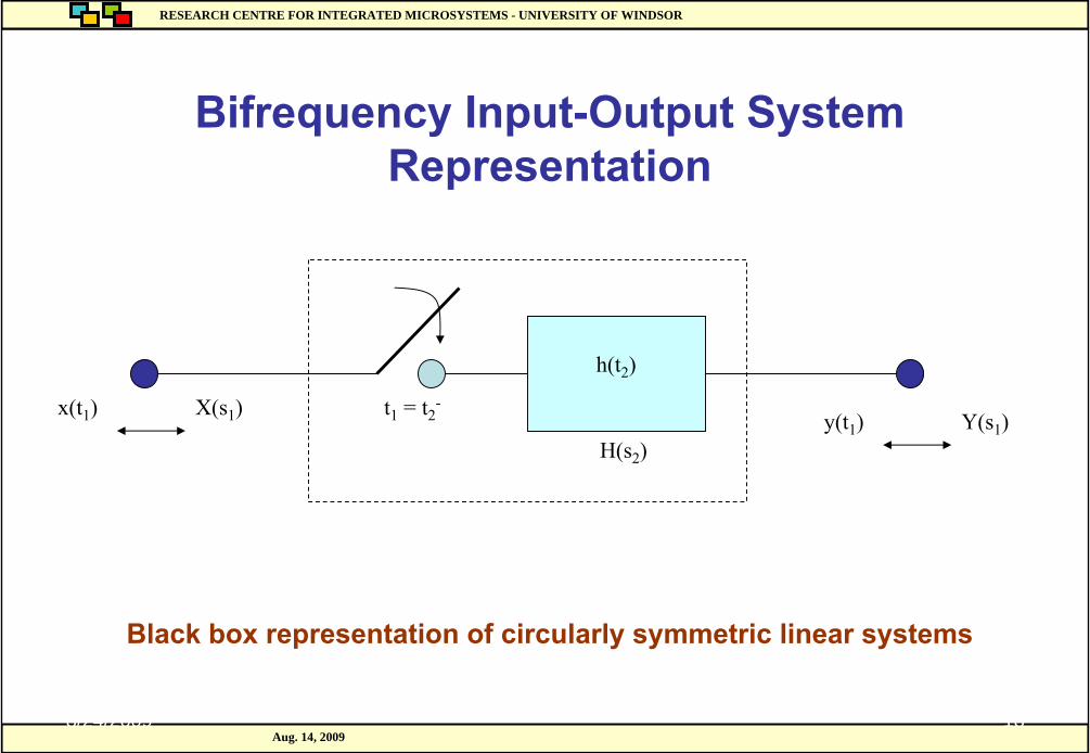
Bifrequency Input-Output System Representation

Black box representation of circularly symmetric linear systems

8/24/2009 18

h(t2)

H(s2)y(t1) Y(s1)

x(t1) X(s1) t1 = t2-


Aug. 14, 2009

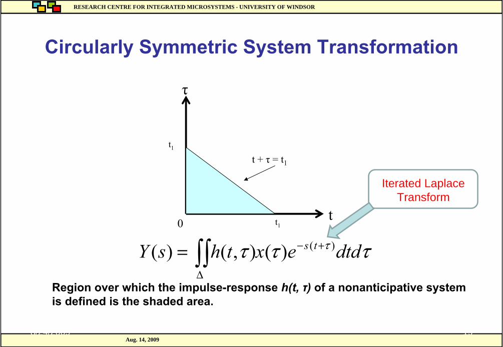
Circularly Symmetric System Transformation

Region over which the impulse-response h(t, τ) of a nonanticipative system is defined is the shaded area.

8/24/2009 19

t1

t1

t

τ

t + τ = t1

0

τττ τ dtdexthsY ts )()(),()( +−

∆∫∫=

Iterated LaplaceTransform


Aug. 14, 20098/24/2009 20

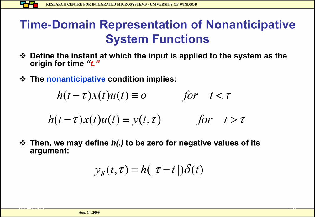
Define the instant at which the input is applied to the system as the origin for time “t.”

The nonanticipative condition implies:

Then, we may define h(.) to be zero for negative values of its argument:

Time-Domain Representation of NonanticipativeSystem Functions

ττ <≡− tforotutxth )()()(

τττ >≡− tfortytutxth ),()()()(

)(|)(|),( tthty δττδ −=


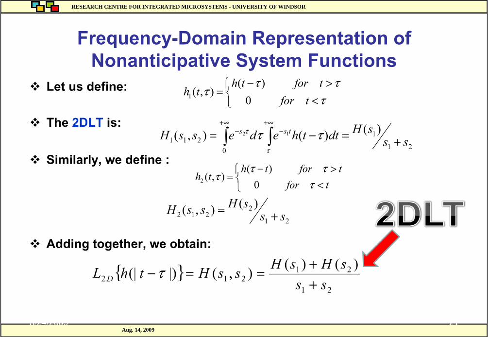
Aug. 14, 20098/24/2009 21

Let us define:

The 2DLT is:

Similarly, we define :

Adding together, we obtain:

Frequency-Domain Representation of Nonanticipative System Functions

⎩⎨⎧

<>−

=τ

τττ

tfortforth

th0

)(),(1

21

1

0211

)()(),( 12

sssHdtthedessH tss

+=−= ∫ ∫+∞ +∞

−− τττ

τ

⎩⎨⎧

<>−

=tfor

tforthth

τττ

τ0

)(),(2

21

2212

)(),( sssHssH +=

{ }21

21212

)()(),(|)(|ss

sHsHssHthL D ++==−τ


Aug. 14, 2009

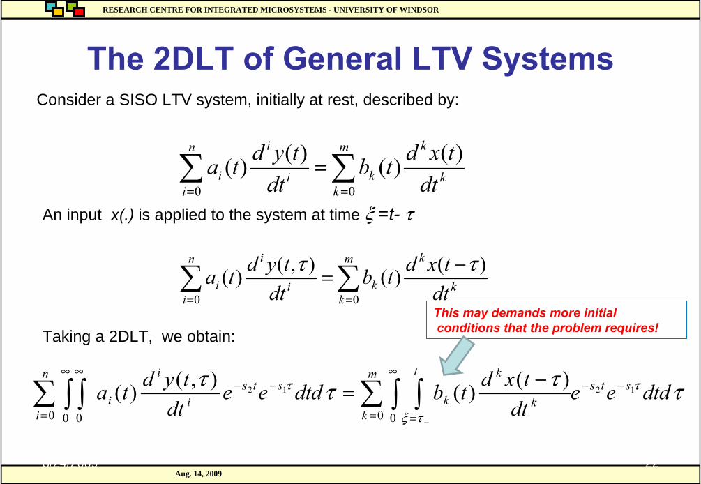
The 2DLT of General LTV Systems

8/24/2009 22

Consider a SISO LTV system, initially at rest, described by:

An input x(.) is applied to the system at time ξ =t- τ

Taking a 2DLT, we obtain:

∑∑==

=m

kk

k

ki

in

ii dt

txdtbdt

tydta00

)()()()(

∑∑==

−=m

kk

k

ki

in

ii dt

txdtbdt

tydta00

)()(),()( ττ

ττττ τ

τξ

τ dtdeedt

txdtbdtdeedt

tydta stsm

kk

k

k

tsts

i

in

ii

1212

0 00 0 0

)()(),()( −−

=

∞

=

−−

=

∞ ∞

∑ ∫ ∫∑ ∫ ∫−=

−

This may demands more initialconditions that the problem requires!


Aug. 14, 2009

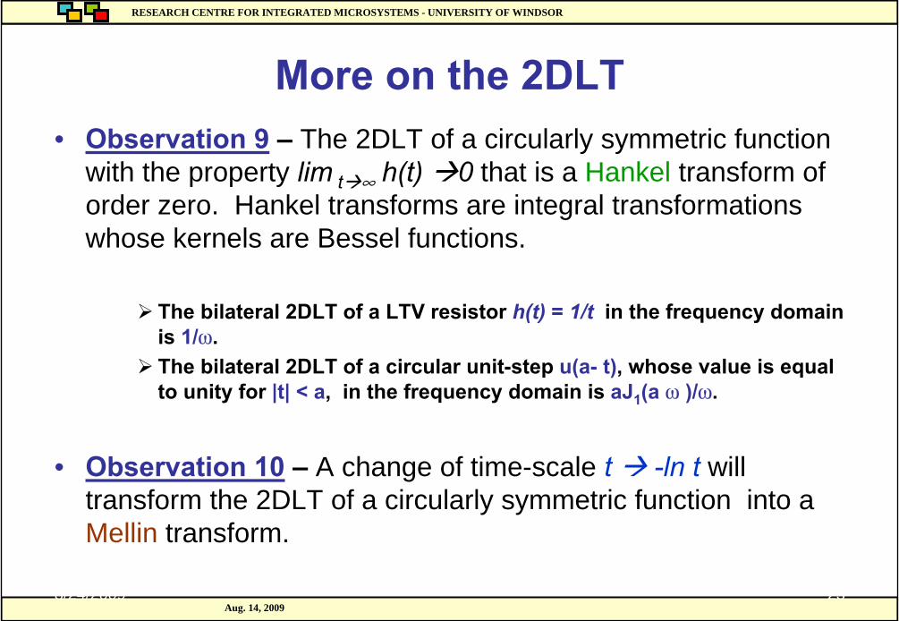
More on the 2DLT• Observation 9 – The 2DLT of a circularly symmetric function

with the property lim t ∞ h(t) 0 that is a Hankel transform of order zero. Hankel transforms are integral transformations whose kernels are Bessel functions.

The bilateral 2DLT of a LTV resistor h(t) = 1/t in the frequency domain is 1/ω.The bilateral 2DLT of a circular unit-step u(a- t), whose value is equal to unity for |t| < a, in the frequency domain is aJ1(a ω )/ω.

• Observation 10 – A change of time-scale t -ln t will transform the 2DLT of a circularly symmetric function into a Mellin transform.

8/24/2009 23


Aug. 14, 20098/24/2009 24

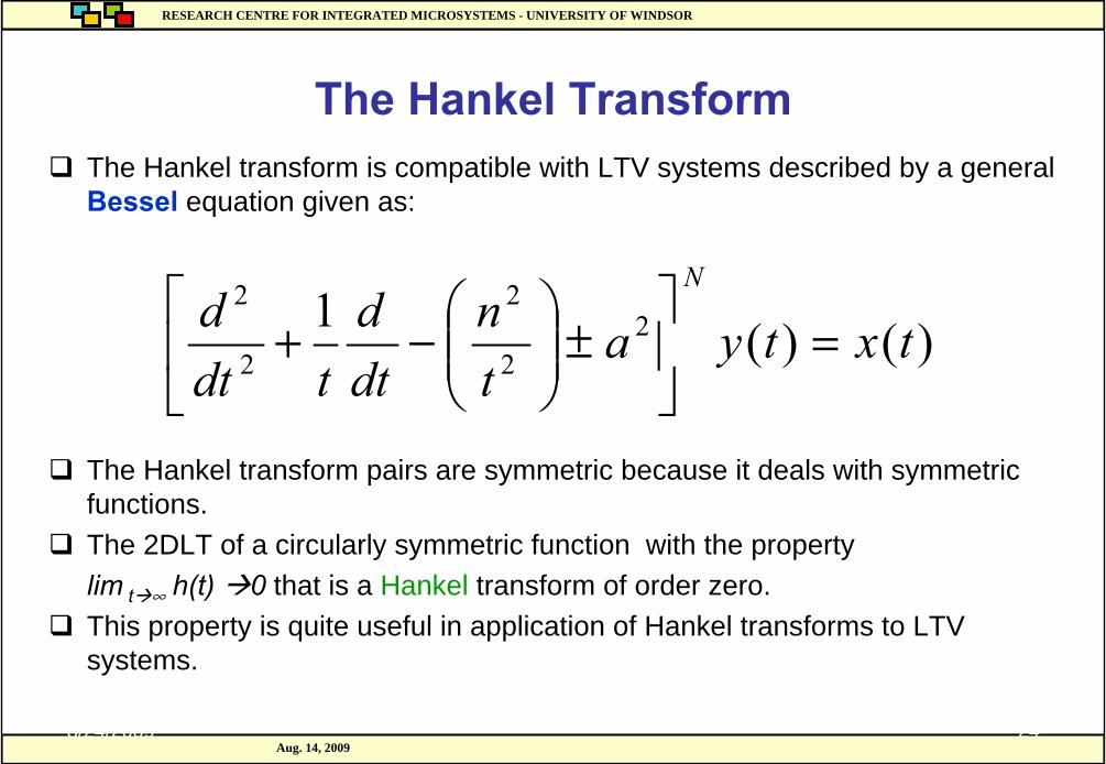
The Hankel transform is compatible with LTV systems described by a generalBessel equation given as:

The Hankel transform pairs are symmetric because it deals with symmetric functions.The 2DLT of a circularly symmetric function with the property lim t ∞ h(t) 0 that is a Hankel transform of order zero.This property is quite useful in application of Hankel transforms to LTV systems.

The Hankel Transform

)()(1 22

2

2

2

txtyatn

dtd

tdtd

N

=⎥⎦

⎤⎢⎣

⎡±⎟⎟

⎠

⎞⎜⎜⎝

⎛−+


Aug. 14, 20098/24/2009 25

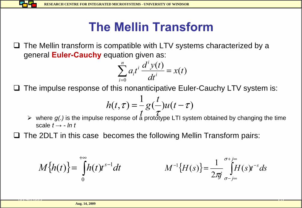
The Mellin transform is compatible with LTV systems characterized by a general Euler-Cauchy equation given as:

The impulse response of this nonanticipative Euler-Cauchy LTV system is:

where g(.) is the impulse response of a prototype LTI system obtained by changing the time scale t → - ln t

The 2DLT in this case becomes the following Mellin Transform pairs:

The Mellin Transform

)()(0

txdt

tydta i

ii

n

ii =∑

=

)()(1),( ττ

τ −= tutgt

th

{ } dttththM s 1

0

)()( −+∞

∫= { } dstsHj

sHM sj

j

−∞+

∞−

− ∫=σ

σπ)(

21)(1


Aug. 14, 2009

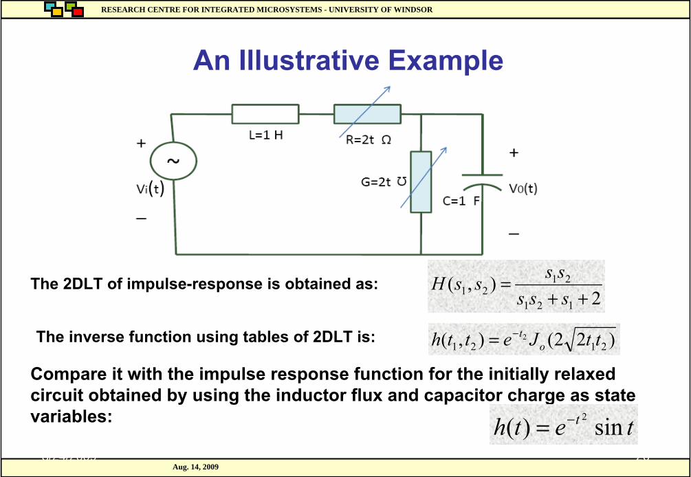
Compare it with the impulse response function for the initially relaxed circuit obtained by using the inductor flux and capacitor charge as state variables:

The 2DLT of impulse-response is obtained as:

8/24/2009 26

An Illustrative Example

The inverse function using tables of 2DLT is:

2),(

121

2121 ++=

sssssssH

)22(),( 21212 ttJetth o

t−=

teth t sin)( 2−=


Aug. 14, 20098/24/2009 27

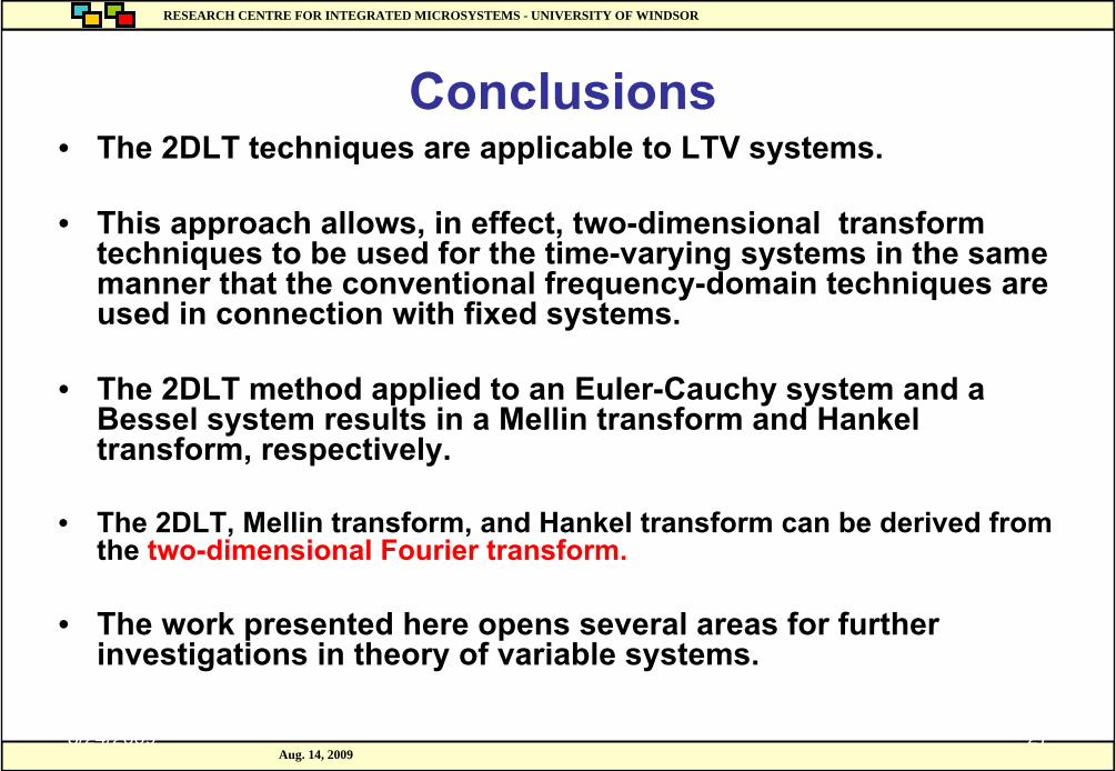
Conclusions• The 2DLT techniques are applicable to LTV systems.

• This approach allows, in effect, two-dimensional transform techniques to be used for the time-varying systems in the same manner that the conventional frequency-domain techniques are used in connection with fixed systems.

• The 2DLT method applied to an Euler-Cauchy system and a Bessel system results in a Mellin transform and Hankeltransform, respectively.

• The 2DLT, Mellin transform, and Hankel transform can be derived from the two-dimensional Fourier transform.

• The work presented here opens several areas for further investigations in theory of variable systems.


Aug. 14, 20098/24/2009 28

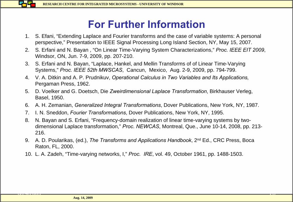
For Further Information1. S. Efani, “Extending Laplace and Fourier transforms and the case of variable systems: A personal

perspective,” Presentation to IEEE Signal Processing Long Island Section, NY, May 15, 2007.2. S. Erfani and N. Bayan , “On Linear Time-Varying System Characterizations,” Proc. IEEE EIT 2009,

Windsor, ON, Jun. 7-9, 2009, pp. 207-210.3. S. Erfani and N. Bayan, “Laplace, Hankel, and Mellin Transforms of of Linear Time-Varying

Systems,” Proc. IEEE 52th MWSCAS, Cancun, Mexico, Aug. 2-9, 2009, pp. 794-799.4. V. A. Ditkin and A. P. Prudnikuv, Operational Calculus in Two Variables and Its Applications,

Pergaman Press, 1962.5. D. Voelker and G. Doetsch, Die Zweirdimensional Laplace Transformation, Birkhauser Verleg,

Basel, 1950.6. A. H. Zemanian, Generalized Integral Transformations, Dover Publications, New York, NY, 1987.7. I. N. Sneddon, Fourier Transformations, Dover Publications, New York, NY, 1995.8. N. Bayan and S. Erfani, “Frequency-domain realization of linear time-varying systems by two-

dimensional Laplace transformation,” Proc. NEWCAS, Montreal, Que., June 10-14, 2008, pp. 213-216.

9. A. D. Poularikas, (ed.), The Transforms and Applications Handbook, 2nd Ed., CRC Press, Boca Raton, FL, 2000.

10. L. A. Zadeh, “Time-varying networks, I,” Proc. IRE, vol. 49, October 1961, pp. 1488-1503.


Aug. 14, 20098/24/2009 29


Aug. 14, 2009

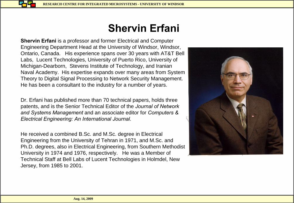
Shervin ErfaniShervin Erfani is a professor and former Electrical and Computer Engineering Department Head at the University of Windsor, Windsor, Ontario, Canada. His experience spans over 30 years with AT&T Bell Labs, Lucent Technologies, University of Puerto Rico, University of Michigan-Dearborn, Stevens Institute of Technology, and Iranian Naval Academy. His expertise expands over many areas from System Theory to Digital Signal Processing to Network Security Management. He has been a consultant to the industry for a number of years.

Dr. Erfani has published more than 70 technical papers, holds three patents, and is the Senior Technical Editor of the Journal of Network and Systems Management and an associate editor for Computers & Electrical Engineering: An International Journal.

He received a combined B.Sc. and M.Sc. degree in Electrical Engineering from the University of Tehran in 1971, and M.Sc. and Ph.D. degrees, also in Electrical Engineering, from Southern Methodist University in 1974 and 1976, respectively. He was a Member of Technical Staff at Bell Labs of Lucent Technologies in Holmdel, New Jersey, from 1985 to 2001.

laplace transformation of linear time-varying systems transformation.pdf · laplace transformation...

Documents