Langmuir Turbulence Parameterization in Tropical Cyclone Conditions

BRANDON G. REICHL

Graduate School of Oceanography, University of Rhode Island, Narragansett, Rhode Island

DONG WANG

College of Earth, Ocean, and Environment, University of Delaware, Newark, Delaware

TETSU HARA AND ISAAC GINIS

Graduate School of Oceanography, University of Rhode Island, Narragansett, Rhode Island

TOBIAS KUKULKA

College of Earth, Ocean, and Environment, University of Delaware, Newark, Delaware

(Manuscript received 8 June 2015, in final form 3 November 2015)

ABSTRACT

The Stokes drift of surface waves significantly modifies the upper-ocean turbulence because of the Craik–

Leibovich vortex force (Langmuir turbulence). Under tropical cyclones the contribution of the surface waves

varies significantly depending on complex wind and wave conditions. Therefore, turbulence closure models

used in ocean models need to explicitly include the sea state–dependent impacts of the Langmuir turbulence.

In this study, the K-profile parameterization (KPP) first-moment turbulence closure model is modified to

include the explicit Langmuir turbulence effect, and its performance is tested against equivalent large-eddy

simulation (LES) experiments under tropical cyclone conditions. First, theKPPmodel is retuned to reproduce

LES results without Langmuir turbulence to eliminate implicit Langmuir turbulence effects included in the

standard KPP model. Next, the Lagrangian currents are used in place of the Eulerian currents in the KPP

equations that calculate the bulk Richardson number and the vertical turbulent momentum flux. Finally, an

enhancement to the turbulent mixing is introduced as a function of the nondimensional turbulent Langmuir

number. The retuned KPP, with the Lagrangian currents replacing the Eulerian currents and the turbulent

mixing enhanced, significantly improves prediction of upper-ocean temperature and currents compared to the

standard (unmodified)KPPmodel under tropical cyclones and shows improvements over the standardKPP at

constant moderate winds (10m s21).

1. Introduction

Tropical cyclone prediction models require sea surface

temperature and currents to accurately compute air–sea

heat and momentum fluxes. These air–sea fluxes are the

primary contributors to the energy budget of a tropical

cyclone and therefore greatly affect the storm intensity

(see Emanuel 1991, 1999). Tropical cyclones are known

to generate vigorous responses in the upper ocean, which

include surface waves with amplitudes larger than 15m,

upper-ocean currents in excess of 1ms21, and sea surface

temperature cooling of several degrees (Ginis 2002). The

surface temperature and current responses to wind forc-

ing are determined by turbulent mixing throughout the

upper-ocean boundary layer, which must be carefully

accounted for in ocean models that are coupled to trop-

ical cyclone forecast models.

As a hurricane passes over a particular location, the

upper-ocean mixing develops in the following manner:

First, near-surface ocean currents and surface waves

increase as momentum from the wind is transferred into

the ocean. The large vertical shear below the developing

surface current generates turbulence and drives the

deepening of the active surface mixing layer. Surface

gravity waves also contribute to the upper-ocean mixing

Corresponding author address: B. G. Reichl, Graduate School of

Oceanography, University of Rhode Island, 215 S. Ferry Rd.,

Narragansett, RI 02882.

E-mail: breichl@my.uri.edu

MARCH 2016 RE I CHL ET AL . 863

DOI: 10.1175/JPO-D-15-0106.1

� 2016 American Meteorological Society

and the turbulent kinetic energy (TKE) budget through

breaking and the Stokes drift; the latter significantly

modifies upper-ocean turbulence (Langmuir turbu-

lence). The near-surface temperature cools due to the

entrainment of cold water from the thermocline below

as the mixing layer deepens (Price 1981). Although

these are primarily one-dimensional (vertical) mixing

processes, the cool-water entrainment under a tropical

cyclone can be further enhanced by three-dimensional

processes, notably by upwelling due to Ekman pump-

ing (Yablonsky and Ginis 2009). Evaporation is an-

other source of surface cooling, although this is

generally a second-order process during strong winds

and active entrainment (Ginis 2002).

In three-dimensional ocean circulation models that

utilize Reynolds-averaged equations of motion, the

upper-ocean turbulent fluxes are typically parameterized

by closure models. The traditional turbulence closure

models (e.g., Mellor and Yamada 1982; Large et al. 1994)

determine the evolution of the mixing layer turbulence

through inputs including the wind stress t (or the friction

velocity u*5ffiffiffiffiffiffiffiffit/ra

p, where ra is the air density) and the

surface buoyancy flux B*. These closure models do not

explicitly capture the contribution of surface gravity

waves to the upper-ocean turbulence. One source of

upper-ocean turbulence due to surface gravity waves is

the injection of TKE from wave breaking to the ocean

(Melville 1996). The elevated turbulence due to breaking

waves decays within depths scaling with the significant

wave height (i.e., Craig and Banner 1994; Terray et al.

1996). Another significant source of turbulence derived

from surface waves is the Langmuir turbulence. The

depth scale of the Langmuir turbulence is typically larger

and is determined by the mixed layer depth and/or the

Stokes drift e-folding depth (Harcourt andD’Asaro 2008;

Grant and Belcher 2009; Sullivan et al. 2012).

First observed by Langmuir (Langmuir 1938), it took

several decades for themechanism that drives Langmuir

circulations to be identified. This is the Craik–Leibovich

(CL) vortex force, which results from interaction be-

tween the Stokes drift of surface waves and the upper-

ocean Eulerian current vorticity (Craik and Leibovich

1976). In the high Reynolds number planetary boundary

layer turbulence, the Langmuir turbulence (turbulence

that is modified by the CL vortex force) exists over

scales ranging from O(1) m to the mixed layer depth,

even when not organized as coherent Langmuir circu-

lations (McWilliams et al. 1997). Langmuir turbulence

has been extensively studied for the last two decades

using large-eddy simulation (LES) models that can re-

solve explicitly the dominant scales of Langmuir tur-

bulence (Skyllingstad and Denbo 1995; McWilliams

et al. 1997; Skyllingstad et al. 2000; Noh et al. 2004; Min

and Noh 2004; Polton and Belcher 2007; Sullivan et al.

2007; Harcourt and D’Asaro 2008; Grant and Belcher

2009; Kukulka et al. 2009; Teixeira and Belcher 2010;

Kukulka et al. 2010; Noh et al. 2011; Van Roekel et al.

2012). All support the conclusion that the CL vortex

force strengthens upper-ocean mixing in many dif-

ferent regimes. Studies that qualitatively and quanti-

tatively compare LES results to in situ data confirm

that including the CL vortex force improves the model

observation agreement (Kukulka et al. 2009; D’Asaro

et al. 2014).

LES has also been used to study stochastic momen-

tum injection via wave breaking in the presence of

Langmuir turbulence in the planetary boundary layer

(Noh et al. 2004; Sullivan et al. 2007; McWilliams et al.

2012). These studies show that the impact of inter-

mittent breaking momentum injection is mostly limited

to the upper several meters when compared to constant

surface momentum fluxes. Therefore, the CL vortex

force (which impacts scales of 10–200m) is a much more

effective mechanism to enhance mixed layer deepening.

Various scalings for the enhancement of the turbulence

closure models based on the Langmuir number have

been proposed, which will be discussed in detail later

(sections 2 and 8).

Sullivan et al. (2012) have employed LES to study

Langmuir turbulence under strong, transient wind stress

and Stokes drift conditions characteristic of tropical cy-

clones. This idealized study shows large variation in

Langmuir turbulence from the right to the left side of the

storm track. The right side of the storm (Northern

Hemisphere convention) has inertially resonant wind and

current rotation, which significantly deepens the mixing

layer compared to the nonresonant left side (Price 1981;

Skyllingstad et al. 2000; Sanford et al. 2011). The right

side also has larger waves due to resonance between the

wind and the storm translation (Young 2003; Moon et al.

2003), which results in a stronger, deeper Stokes drift

profile (Sullivan et al. 2012).

Recently, Rabe et al. (2015) investigated Langmuir

turbulence under Hurricane Gustav (2008) by combin-

ing in situ measurements of turbulence obtained by

Lagrangian floats deployed ahead of the storm and LES

hindcasts of the upper-ocean turbulence at the float lo-

cations. The observations show a regime behind the eye

of a tropical cyclone where the turbulent vertical ve-

locity variance w02 is reduced compared to traditional

wind-driven u* scaling. The LES results suggest that

such a regime may be due to large variability of the

Langmuir turbulence, since the local wave field varies

significantly (both in time and in space) under a tropical

cyclone. Comparisons between the turbulent quantities

from the LES and the observations are imperfect for

864 JOURNAL OF PHYS ICAL OCEANOGRAPHY VOLUME 46

various reasons, particularly because of uncertainty of

the drag coefficient in tropical cyclone conditions (see

Rabe et al. 2015). Nevertheless, the results suggest that

the Langmuir turbulence is an important, spatially var-

iable source of mixing under a tropical cyclone and that

the additional mixing due to the CL vortex force is

necessary to best match the simulations and the field

observations.

To improve the comparison between models con-

taining the Langmuir turbulence and in situ data,

large-scale three-dimensional processes such as up-

welling and advection must be included. However,

such models are computationally expensive and can-

not be run at resolutions that are needed to resolve the

dominant Langmuir turbulence scale. Therefore, tur-

bulence closure models that parameterize Langmuir

turbulence must be developed and be included in

coarse-resolution [O(103–104)m] basin-scale numeri-

cal ocean models. Such an approach would contribute

to improved performance of coupled hurricane–

wave–ocean simulation/prediction models.

The main objective of this study is to develop a robust

turbulence closure model that accurately accounts for

the Langmuir turbulence effects under tropical cyclone

conditions. Such a model is constructed and tested using

an extensive set of LES Langmuir turbulence experi-

ments under a wide range of tropical cyclone wind and

wave conditions.

2. Geophysical turbulence closure models

In typical ocean models based on Reynolds-averaged

Navier–Stokes (RANS) equations, the horizontal mo-

mentum equations, with the hydrostatic and Boussinesq

approximations, can be expressed as

›Uh

›t1

�U

h� ›

›xh

1W›

›z

�U

h1 f3U

h

521

r0

›P

›xh

2›

›z

�n›U

h

›z1 u0

hw0�, (1)

where xh are the horizontal coordinates, z is the ver-

tical coordinate (positive upward), f is the Coriolis

parameter (vector), n is the molecular viscosity, and

r0 is the reference density. The instantaneous hori-

zontal velocity vector uh and vertical velocity w are

decomposed into the Reynolds mean (Uh, W ) and

fluctuation (u0h, w

0), and P is the Reynolds-averaged

dynamic pressure. The overbar represents the Rey-

nolds mean, and u0hw

0 is the vertical turbulent mo-

mentum flux. The horizontal turbulent fluxes have

been neglected. The temperature advective–diffusive

equation can be expressed as

›Q

›t1U

h� ›Q›x

h

1W›Q

›z52

›

›z

�nu

›Q

›z1 u0w0

�, (2)

where the potential temperature u is similarly decom-

posed into the Reynolds mean Q and fluctuation u0, andnu is the molecular diffusion of heat. Again, horizontal

turbulent fluxes have been dropped.

In the presence of the wave-induced Stokes drift profile

uS, the advective and planetary terms in the momentum

equation contain the Stokes drift (following McWilliams

and Restrepo 1999):

›Uh

›t1

�U

h� ›

›xh

1W›

›z

�U

h1 f3 (U

h1u

S)

1v3uS52

1

r0

› ~P

›x2

›

›z

�n›U

h

›z1 u0

hw0�, (3)

where v 5 = 3 Uh is the vertical (relative) vorticity

vector, the advective Stokes drift component is repre-

sented through the vortex force v 3 uS, the planetary

rotation term is modified to include the Stokes drift (the

Coriolis–Stokes term), and the dynamic pressure ~P has

been modified to include the Stokes drift correction.

Similarly, the Stokes drift is introduced to the advective

terms of the temperature equation

›Q

›t1 (U

h1 u

S) � ›Q

›xh

1W›Q

›z52

›

›z

�nu

›Q

›z1 u0w0

�.

(4)

The Stokes drift should be calculated from the full

wave spectra, which are prescribed based on observations

or surface wave models. Therefore, the only components

of the system that cannot be solved for by the horizontal

momentum equation [(3)], the temperature–advection

equation [(4)], the equation of state, and the continuity

equation are the vertical turbulent flux terms. A turbu-

lence closure model is used to calculate these terms,

which can be expressed as

u0hw

0 52KM

›Uh

›z1G

U, and (5)

u0w0 52Ku

›Q

›z1G

u, (6)

where the vertical turbulent flux of a property is equal to

the vertical gradient of the mean property multiplied by

an eddy viscosity KM (or an eddy diffusivity Ku for

temperature) plus a nonlocal (or countergradient) term

G. The K-profile parameterization (KPP; Large et al.

1994) is one example of a turbulent closure model for

geophysical applications that solves for the turbulent

fluxes following this form. Recently, several studies

MARCH 2016 RE I CHL ET AL . 865

(McWilliams and Sullivan 2000; Smyth et al. 2002;

McWilliams et al. 2012, 2014; Sinha et al. 2015) proposed

modifications to the KPP model that include the Lang-

muir turbulence.

In McWilliams and Sullivan (2000), the Langmuir

turbulence is included via an enhancement factor to

the eddy viscosity (and diffusivity) through an en-

hanced turbulent velocity scale. The enhancement

factor is parameterized from the turbulent Langmuir

number:

Lat5

ffiffiffiffiffiffiffiffiffiffiffiffiffiffiffiffiffiffiffiffiffiffiu*

juS(z5 0)j

s, (7)

where juS(z5 0)j is the magnitude of the surface Stokes

drift. This approach was later modified by Smyth et al.

(2002) to include dependency on the surface buoyancy

flux. Fan and Griffies (2014) showed that using this en-

hanced turbulent velocity scale in the MOM global

ocean circulation model had significant impacts on the

evolution of the temperature and mixed layer depth in

certain regions. However, the enhanced velocity scale

did not properly resolvemodel differences against in situ

observations, suggesting the need for additional model

improvements.

McWilliams et al. (2012) proposed further modifica-

tions to the KPP model that include an additional

component of the turbulent momentum flux down the

gradient of the Stokes drift:

u0hw

0 52KL

›UhL

›z, (8)

where KL is the Lagrangian eddy viscosity, and UhL is

the Lagrangian current (UhL5 uS1Uh). This approach

was demonstrated to improve simulations of the mean

current profiles in idealized, unstratified conditions

when compared to LES. McWilliams et al. (2014) sug-

gest that for more accurate prediction of the mixing

depth the KPP model may also require enhancement of

the turbulent velocity scale to compute the unresolved

contributions to the bulk mixed layer shear.

Other studies investigated second-moment turbu-

lence closure models by including the CL vortex force in

the TKE equation (D’Alessio et al. 1998), the dissipa-

tion length scale (Kantha and Clayson 2004), and the

stability functions (Harcourt 2013, 2015). The additional

turbulent flux down the gradient of the Stokes drift is a

key component to the modifications presented by

Harcourt (2013, 2015). These studies demonstrate that

prediction of the upper-ocean current is improved if the

Langmuir turbulence parameterization via Stokes drift

is included in the closure model.

In this study we focus on the KPP turbulence closure

model under tropical cyclone conditions. First, the per-

formance of the standard KPP model without explicit

Langmuir turbulence effects is investigated under tropi-

cal cyclone conditions. Next, we investigate how different

modifications to the KPP model that include Langmuir

turbulence improve the comparison with equivalent LES

simulations.

3. Experimental design

Although anymodel performance should be validated

against observations in principle, it is difficult to test the

KPP model using in situ data in tropical cyclone condi-

tions. Reliable observational data are extremely rare in

high-wind environments. Furthermore, to test the KPP

model it is preferable to utilize one-dimensional exper-

iments (where horizontal variations are neglected) in

order to isolate the vertical turbulent mixing from large-

scale three-dimensional processes that introduce addi-

tional complications. In situ observations are inherently

three-dimensional and lack the temporal and spatial

distributions needed to properly test the KPP model

over a robust range of conditions. Instead, we will vali-

date the KPP model against idealized computational

experiments using a LES model that explicitly resolves

the Langmuir turbulence. The performance of the KPP

model embedded in a one-dimensional RANS model is

tested against the one-dimensional solutions derived by

horizontally averaging the LES results.

The ocean surface waves are simulated using the

WAVEWATCH III (WW3; Tolman 2009) surface

wave model. The WW3 (v3.14) model is used with a

modification to the wind input source function that has

been demonstrated to well predict the peak wave

spectrum under tropical cyclone conditions (Fan et al.

2009). The computational domain has a uniform deep-

water (4000m) bathymetry. The horizontal dimensions

are 1800 km in the direction perpendicular to the storm

translation and 3000 km in the direction of storm

translation, which are large enough that the boundaries

are not dynamically important to the study location.

The horizontal resolution of the wave model is 8.33 km,

and the wave spectrum is defined over 40 logarithmi-

cally spaced frequencies (with a minimum frequency of

0.0285Hz) and 48 evenly spaced directions. Surface

forcing is applied using a defined, idealized tropical

cyclone wind stress. The wind field is constructed fol-

lowing the model of Holland (1980) with a realistic

wind inflow angle model following Zhang and Uhlhorn

(2012). The radius of maximum wind (RMW) is set as

50 km, and the maximum wind speed is set at 65m s21.

The wave field is initially at rest.

866 JOURNAL OF PHYS ICAL OCEANOGRAPHY VOLUME 46

The identical wind stress is applied in the LES and

one-dimensional RANS models, which are calculated

using the bulk formula with the drag coefficient formu-

lation as Sullivan et al. (2012):

Cd5

8<:0:0012, : ju

10j, 11m s21

(0:491 0:065ju10j)3 1023 , : 11m s21 # ju

10j# 20m s21

0:0018, : 20m s21 , ju10j

, (9)

where ju10j is the neutral 10-m windmagnitude. A very

weak (5Wm22) destabilizing surface buoyancy flux is

also applied, which is insignificant after the initial

onset of turbulence. Even a realistic surface heat flux

does not significantly contribute to the turbulent

mixing within the peak region of a tropical cyclone

(wind speeds greater than ;15m s21). We therefore

neglect this contribution.

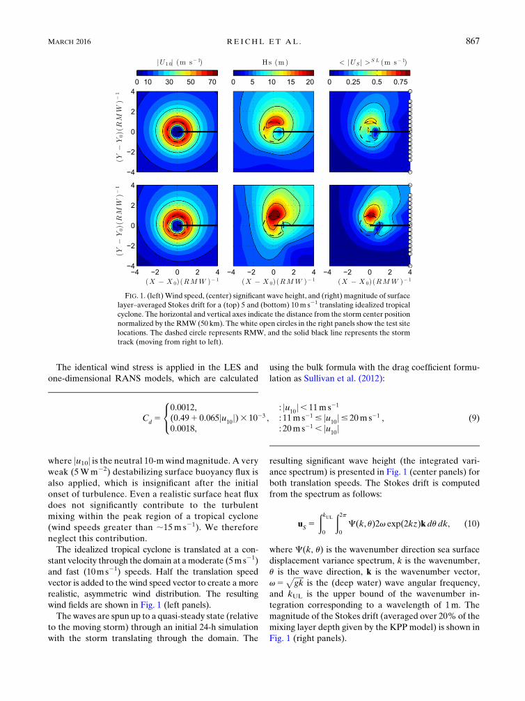
The idealized tropical cyclone is translated at a con-

stant velocity through the domain at amoderate (5ms21)

and fast (10ms21) speeds. Half the translation speed

vector is added to the wind speed vector to create a more

realistic, asymmetric wind distribution. The resulting

wind fields are shown in Fig. 1 (left panels).

The waves are spun up to a quasi-steady state (relative

to the moving storm) through an initial 24-h simulation

with the storm translating through the domain. The

resulting significant wave height (the integrated vari-

ance spectrum) is presented in Fig. 1 (center panels) for

both translation speeds. The Stokes drift is computed

from the spectrum as follows:

uS5

ðkUL

0

ð2p0

C(k, u)2v exp(2kz)k du dk, (10)

where C(k, u) is the wavenumber direction sea surface

displacement variance spectrum, k is the wavenumber,

u is the wave direction, k is the wavenumber vector,

v5ffiffiffiffiffiffigk

pis the (deep water) wave angular frequency,

and kUL is the upper bound of the wavenumber in-

tegration corresponding to a wavelength of 1m. The

magnitude of the Stokes drift (averaged over 20% of the

mixing layer depth given by the KPP model) is shown in

Fig. 1 (right panels).

FIG. 1. (left) Wind speed, (center) significant wave height, and (right) magnitude of surface

layer–averaged Stokes drift for a (top) 5 and (bottom) 10m s21 translating idealized tropical

cyclone. The horizontal and vertical axes indicate the distance from the storm center position

normalized by the RMW (50 km). The white open circles in the right panels show the test site

locations. The dashed circle represents RMW, and the solid black line represents the storm

track (moving from right to left).

MARCH 2016 RE I CHL ET AL . 867

The 20 test locations perpendicular to the translation

direction are selected. They are given in Table 1 and

plotted for reference in Fig. 1 as white circles in the right

panels. At each location the time series of the wind stress

andwaves are used to force theLESand one-dimensional

RANS models. An additional test is conducted to assess

the performance of the model in lower wind conditions.

A constant 10ms21 wind is applied over the entire do-

main. The fully developed (steady state) wave spectrum

at a fetch of 2000km is used to calculate a Stokes drift

profile. The LES and one-dimensional models then cal-

culate the turbulence and mean ocean properties for 24h

with this Stokes drift input, which is held constant. This

ensures that waves are neither time or fetch limited for

the constant wind experiments.

For the tropical cyclone experiments, one-dimensional

and LES simulations are performed for 48 h, with the

wind maximum occurring at 36 h. Comparison between

the two models is performed for a duration of 24 h at

each location, from 12h before the wind maximum to

12 h after the wind maximum. This restricts the com-

parison between the one-dimensional simulation and

the LES model to periods with higher wind. The initial

potential temperature profile has a homogenous mixed

layer of u 5 29.258C and a constant stratification in the

interior of 20.04 8Cm21, which are identical to Sullivan

et al. (2012). Two initial mixed layer depths are

investigated, a shallower depth of 10m and a deeper

depth of 32m. The simulations are performed across all

20 test locations for the 10-m depth and at 11 stations for

the 32-m depth. The 32-mmixed layer depth is chosen to

correspond to the Sullivan et al. (2012) experiment,

while the 10-m mixed layer depth is chosen as a rea-

sonable upper limit for a shallow, summer mixed layer.

For the constant wind simulation the initial mixed layer

depth is 10m, but the stratification is reduced to

20.018Cm21.

The LES and one-dimensional RANS model are run

with identical forcing, physical parameters, and the lin-

ear equations of state, which is defined as

r5 r01a(u2 u

0) , (11)

where the reference density r0 is 1026.95kgm23 for u0 5

108C and the salinity S 5 35psu. The salinity is kept

constant and the thermal expansion coefficient is

a520.2kgm23 (8C)21. For the one-dimensional model,

the General Ocean Turbulence Model (GOTM; Umlauf

et al. 2005) is used, which includes the Coriolis–Stokes

force and a modified KPP routine to account for the

Langmuir turbulence.

The LES domain for the tropical cyclone experiments

is (x, y, and z)5 (750, 750, and 240m) with a resolution

of (dx, dy, and dz) 5 (2.92, 2.92, and 1m). For the

constant wind experiment, a smaller domain is used with

(x, y, and z) 5 (300, 300, and 180m) and a resolution of

(dx, dy, and dz) 5 (1.56, 1.56, and 0.7m). Our previous

sensitivity tests indicated that a higher resolution or a

larger domain size does not substantially change our

results, indicating that our resolution is adequate. We

also assessed the TKE partitioning between resolved

and subgrid scale (SGS). The resolved TKE is usually

greater than 75% of the total (resolved 1 SGS) TKE,

which also supports that our resolution is sufficient. The

LES model solves the SGS-averaged equations of mo-

mentum, density, and continuity following previous LES

Langmuir turbulence studies (McWilliams et al. 1997).

The phase-averaged momentum equations are solved in

the three-dimensional coordinate system:

Du

Dt1 f z3 (u1 u

S)

52=p2 gz

�r

r0

�1 u

S3 (=3 u)1 SGS, (12)

where the model variables are SGS averaged, D/Dt 5›/›t 1 u � ›/›x, x is the coordinate vector, u is the ve-

locity vector, uS is the Stokes drift vector (the vertical

component is set to 0), f is the Coriolis parameter, p is

the generalized pressure [p/r1 0.5(ju1 uSj22 juj2)], pis the pressure, and SGS are the subgrid-scale terms

described in detail by Rabe et al. (2015). Scalar

(temperature) distribution is solved by the advective–

diffusive equation:

Dr

Dt1u

S� =r5 SGS, (13)

where r is the density [determined entirely by the tem-

perature via Eq. (11)]. Volume conservation is ensured

via the incompressible continuity equation:

TABLE 1. Location of 20 test sites for one-dimensional and LES models.

Site number 1a 2a 3a 4a 5a 6a 7a 8a,b 9a,b 10a,b

Location (km) 300 200 150 130 110 90 70 50 30 10

Site number 11a,b 12a,b 13a,b 14a,b 15a,b 16a,b 17a,b 18a 19a,b 20a

Location (km) 0 220 240 260 280 2100 2120 2140 2200 2300

a 10-m mixed layer.b 32-m mixed layer.

868 JOURNAL OF PHYS ICAL OCEANOGRAPHY VOLUME 46

= � u5 0. (14)

The Stokes drift is included in themomentumequation via

the Stokes–Coriolis force [term two on the LHS of Eq.

(12)], the CL vortex force [term three on the RHS of Eq.

(12)], and the generalized pressure. The Stokes drift also

contributes to the temperature equation via the additional

Stokes drift advection term. In general, the Langmuir

turbulence has amuch greater impact on themean current

profile than the Stokes–Coriolis force.

The LES is initialized in a similar manner as that de-

scribed by Rabe et al. (2015). In each case, the stationary

simulation is run with the initial wind, wave, and density

profile until statistically stationary turbulence is achieved

(e.g., for multiple eddy turnover times; h/u*). The re-

sulting field is then used as the initial condition for the

transient LES simulation. Unlike Rabe et al. (2015),

however, the mean current in the stationary solution is

removed from the initial condition, such that the initial

mean current is zero in both the LES and the one-

dimensional model.

The LES model is first run at each test location with

the Stokes drift set to zero. This means that both the

Langmuir turbulence and the Coriolis–Stokes force are

not simulated and the turbulence is primarily driven by

vertical current shear. The results from these simula-

tions are referred to as LES–shear turbulence (ST).

Next, the LES model is run at each location with the

Stokes drift computed from the WW3 wave variance

spectrum. The Stokes drift profile is calculated di-

rectly from the spectrum on the LES model vertical

grid levels and linearly interpolated from the WW3 to

the LES model time step. The results of these simu-

lations will be referred to as LES–Langmuir turbu-

lence (LT). The LES results are averaged horizontally

into vertical profiles for comparing with results in the

one-dimensional model.

4. LES results

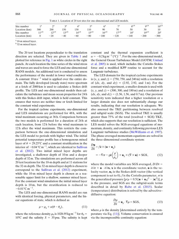
In Fig. 2, we present the difference between the mean

near-surface fields (temperature and currents at 5-m

depth) in LES–LT and LES–ST for the tropical cyclone

with 5m s21 translation speed and the 10-m initial mixed

layer depth. The results with the larger translation speed

and/or the deeper initial mixed layer depth are qualita-

tively similar. Although the actual simulations are con-

ducted over time at fixed locations, we use the time and

translation speed of the storm to transform from the

temporal coordinate to the spatial coordinate (in the

direction of the storm translation) to simplify the pre-

sentation. This transformation is possible because all

results are presented after the wave field has reached a

quasi-steady state with respect to the frame of reference

FIG. 2. (top) LES results of near-surface (at 5-m depth) current magnitude and (bottom)

temperature anomaly (temperature minus initial temperature) for a 5m s21 translating

tropical cyclone. The results are shown for (left) LES–ST, (center) LES–LT, and (right) the

difference between the two. Note the white regions in the upper-right panel have small

negative values. The horizontal and vertical axes indicate the distance from the storm center

position normalized by the RMW (50 km).

MARCH 2016 RE I CHL ET AL . 869

moving with the storm. Since our simulations are

performed with a reasonably high spatial resolution in

the direction perpendicular to the storm translation

(Fig. 1), we can present the spatial snapshots of the

current and temperature fields in Fig. 2. These spatial

patterns remain independent of time after the wave field

has reached quasi-steady state.

The contribution of Langmuir turbulence to cooling is

greatest near the location of maximum Stokes drift

shown in Fig. 1. The additional cooling due to Langmuir

turbulence reaches a maximum of nearly 0.48C on the

right-hand side in a region where the total cooling is

between 2.58 and 38C. This is the region where the peak

waves are longest and the Stokes drift penetrates deep-

est into the water column. This is also the location of

rapid mixed layer deepening, suggesting that Langmuir

turbulence is a significant contributor to the deepening

of the mixing layer. The region of significant enhanced

cooling (0.18C or more) due to Langmuir turbulence is

quite large, extending to about 3 (2) times the RMW to

the right (left).

The near-surface current magnitude in LES–LT is

smaller by as much as 0.7m s21 than that in LES–ST

near the location of the maximum current. The Lang-

muir turbulence significantly increases the turbulent

momentum transport within the upper portion of the

water column where the Stokes drift and its vertical

gradient are greatest. There is a small location near the

center and in the left rear of the hurricane where the

currents are slightly stronger in the presence of

Langmuir turbulence. Overall, Langmuir turbulence

has a more noticeable impact on the mixing of currents

than temperature in the upper water column, since the

current gradients are strong, but temperature is well

mixed and nearly uniform. This does not imply that the

contribution to surface cooling is trivial, since even a

temperature change of O(0.1) 8C may have significant

implications for the tropical cyclone development

(Emanuel 1999).

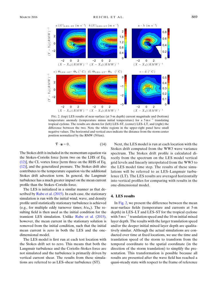
To demonstrate the vertical dependence of the

Langmuir turbulence impact in this study, we present

vertical transects of the upper-ocean current magnitude

and temperature from 50km to the right of the storm

center (Fig. 3). The current is significantly decreased

near the surface in LES–LT compared to the LES–ST in

the area where the Stokes drift is large and the Langmuir

turbulence is strong. The difference between the LES–

LT and LES–ST currents decreases gradually from the

surface down to about 50m, suggesting that the impact

of the Langmuir turbulence penetrates quite deep

compared to the Stokes drift itself, which mostly decays

within 10m or so from the surface. Near the base of the

mixing layer the LES–LT current is greater than the

LES–ST currents, which is due to the increased mixing

depth in LES–LT. The LES–LT temperature is cooler

than the LES–ST temperature down to about 100m, but

there is less vertical dependence of the temperature

difference compared to the current difference. At the

FIG. 3. LES transect (at 50 km to right of storm center) of (top) current magnitude and

(bottom) temperature for a 5m s21 translating tropical cyclone. The results are shown for

(left) LES–ST, (center) LES–LT, and (right) the difference between the two. The horizontal

axes indicate the distance from the storm center position normalized by the RMW (50 km).

870 JOURNAL OF PHYS ICAL OCEANOGRAPHY VOLUME 46

base of the mixing layer the LES–LT is warmer than

LES–ST due to the increased mixing depth.

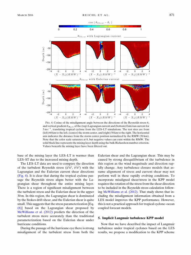
The LES–LT data are used to compare the direction

of the turbulent Reynolds stress (u0w0, y0w0) with the

Lagrangian and the Eulerian current shear directions

(Fig. 4). It is clear that during the tropical cyclone pas-

sage the Reynolds stress aligns better with the La-

grangian shear throughout the entire mixing layer.

There is a region of significant misalignment between

the turbulent stress and the Eulerian shear in the upper

30m. In this region, the Lagrangian shear is dominated

by the Stokes drift shear, and the Eulerian shear is quite

small. This suggests that the stress parameterization [Eq.

(8)] based on the Lagrangian shear proposed by

McWilliams et al. (2012) predicts the direction of the

turbulent stress more accurately than the traditional

parameterization based on the Eulerian shear under

hurricane conditions.

During the passage of the hurricane eye there is strong

misalignment of the turbulent stress from both the

Eulerian shear and the Lagrangian shear. This may be

caused by strong disequilibrium of the turbulence in

this region as the wind magnitude and direction rap-

idly change. Any turbulence closure models that as-

sume alignment of stress and current shear may not

perform well in these rapidly evolving conditions. To

incorporate misaligned shear/stress in the KPP model

requires the rotation of the stress from the shear direction

to be included in the Reynolds stress calculation follow-

ing McWilliams et al. (2012). That study shows that in-

cluding the misalignment information obtained from a

LES model improves the KPP performance. However,

this is not a practical approach for tropical cyclone–ocean

coupled forecast models.

5. Implicit Langmuir turbulence KPP model

Now that we have described the impact of Langmuir

turbulence under tropical cyclones based on the LES

results, we propose a modification to the KPP scheme

FIG. 4. Cosine of the misalignment angle between the directions of the Reynolds stress utand vertical gradient u›Uh/›z of the (top) Lagrangian current and (bottom)Eulerian current for

5m s21, translating tropical cyclone from the LES–LT simulations. The test sites are from

(left) 60 km to the left, (center) the storm center, and (right) 50 km to the right. The horizontal

axis indicates the distance from the storm center position normalized by the RMW (50 km).

Note that the color scale saturates at 0, but negative values can exist within the RMW. The

solid black line represents themixing layer depth using the bulkRichardson number criterion.

Values beneath the mixing layer have been filtered out.

MARCH 2016 RE I CHL ET AL . 871

that can reproduce the LES–LT results in the one-

dimensional model. This modification will proceed in

the following manner. First, we demonstrate that the

standard KPP scheme, which implicitly includes the typ-

ical (sea state independent) Langmuir turbulence impact,

is not adequate to reproduce the simulated temperature

and currents from the LES–LT (this section). Next, we

remove the implicit Langmuir turbulence impact from

the KPP model so that the one-dimensional simulation

accurately reproduces the LES–ST results (section 6).We

then introduce the explicit Langmuir turbulence impact

in two steps. In step one, we replace the Eulerian cur-

rent with the Lagrangian current in KPP because the

LES results have clearly demonstrated that the turbu-

lent fluxes are more closely aligned to the Lagrangian

shear than the Eulerian shear. We find that this step

does not produce enough mixing in the KPP model

compared to the LES–LT (section 7). In step two, we

introduce enhancement factors of the turbulent mixing

coefficient and the unresolved shear in KPP so that the

one-dimensional simulations best agree with the LES–

LT results (section 8).

a. Method

We first investigate the performance of the standard

KPP model (without explicit Langmuir turbulence ef-

fects) in tropical cyclone conditions. We define the

standard KPP model following Large et al. (1994) in

which the turbulent fluxes are calculated as the product

of the eddy viscosityKM (or diffusivityKu) and themean

vertical gradient of the momentum (or scalar) plus an

additional nonlocal (countergradient) component [Eqs.

(5) and (6)]. Because our experiments include only an

insignificant surface buoyancy flux, the nonlocal com-

ponents are neglected.

The vertical profile of Kx (where x can be u orM) is a

function of normalized depth s 5 2z/h, where h is the

mixing layer depth (which is defined for KPP later in this

section). With the countergradient term dropped,Kx(s)

is equal to the product of the mixing layer depth h, the

turbulent velocity scaleWx, and a nondimensional shape

function Gx(s):

Kx(s)5 hW

xG

x(s) . (15)

The nondimensional turbulent mixing shape function is

approximated by a cubic polynomialGx(s)5 a0 1 a1s 1a2s

2 1 a3s3. The coefficients are determined following

arguments of Large et al. (1994), where a0must be equal to

zero (turbulent eddies do not cross the surface), a1 equals

one (to match the near-surface value ofKx ;2ku*z), and

a2 and a3 can be determined by matching the value and

curvature ofKx to the interior. Since the interior turbulent

mixing parameter is negligible in this study, a2;22 and

a3; 1; thus,Gx(s); s(12 s)2 for bothmomentum and

temperature. The turbulent velocity scale is Wx 5u*k/fx(sh/L), where k is the von Kármán constant, fx is

the universal stability function, and L is the Monin–

Obhukhov length u3

*/(kB*). In this study, L � h and

Wx ; u*k for both momentum and temperature.

Therefore, Kx, Wx, and Gx are all identical for temper-

ature and momentum.

The mixing layer depth h is calculated by the KPP

model using a bulk Richardson number Rib threshold,

which compares the relative contribution of stabilizing

buoyancy and destabilizing shear:

Rib(z)5

[Br 2B(z)]jzj[Ur 2U(z)]2 1 [Vr 2V(z)]2 1V2

t (z),Ri

c,

(16)

where B is the buoyancy, Vt is the unresolved turbulent

velocity shear, and the superscript r denotes a reference

value. At the bottom of the mixing layer Rib(z52h)5Ric. The Ekman depth (hE ; 0:7u*/f ), which is impor-

tant when stratification is weak, and the Monin–

Obhukov depth (hMO 5L5 u3

*/B*k), which is impor-

tant during surface heating (restratification) events,

further restrict this mixing layer. The value of Ric varies

based on the model resolution, but a typical value is 0.3.

The unresolved turbulence term contains the contribu-

tion of convection to mixing:

V2t (z)5

Cy(2b

T)1/2

Rick2

(cs�)21/2jzjNW

u, (17)

whereN is the stability frequency and the constants are

Cy 5 1.6, bT 5 20.2, cs 5 98.96, and � 5 0.1, following

Large et al. (1994). ThisV2t term should also include the

unresolved Langmuir turbulence contribution to

deepening the mixing layer (McWilliams et al. 2014).

The reference variables in the bulk Richardson number

(Ur, Vr, and Br) are defined as the average over the

upper 10% of the mixing layer, following Large et al.

(1994) and Griffies et al. (2013). This averaging is a

standard procedure because it reduces the resolution

dependence of the bulk Richardson number. We also

find that this averaging prevents overpredicting the

mixing depth when the current is surface intensified,

particularly under extreme wind speeds.

This version of KPP with Ric 5 0.3 is defined as the

implicit Langmuir turbulence (iLT) version for this

study (hereinafter KPP–iLT) (see Table 2 for the list of

all KPP experiment descriptions). It should be noted

that this version of the model implicitly includes mean

wave impacts (including Langmuir turbulence) because

872 JOURNAL OF PHYS ICAL OCEANOGRAPHY VOLUME 46

the coefficients (particularly Ric) have been determined

empirically from in situ data and the real ocean always

contains waves when there is significant wind.

b. Results

We first compare the mean near-surface (z 5 25m)

values of both temperature anomaly (where the initial

temperature is subtracted from the simulated tempera-

ture) and currents. We evaluate the results at the near-

surface since this is most relevant for the hurricane

modeling application, but the conclusions are essentially

the same if we choose a deeper (z5230m) transect for

comparison. The root-mean-square difference between

the KPP (one-dimensional GOTM) and LES results is

used as a metric to evaluate the KPP performance. RMS

difference is computed over 24 h (612h relative to the

passage of the peak winds) in all test experiments (both

translation speeds, both initial mixed layer depths) and

at all locations. For the 5ms21 translating storm this

corresponds to the spatial study transect of 432 km, and

for the 10m s21 translating storm this corresponds to the

spatial study transect of 864km. As long as the time and

location are consistent, this is a useful metric to compare

different KPP methods within this study. Note that be-

cause both the LES and the one-dimensional model are

initialized with zero mean current, the phases of the

inertial oscillations remain almost identical between the

two models.

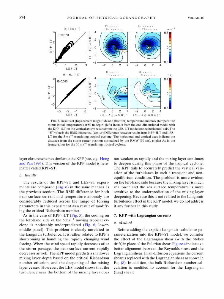
The results of the KPP–iLT and LES–LT experiments

are compared in Fig. 5. All results (both initial mixed

layer depths and both translation speeds) are included in

the left panels. The small difference in the temperature

anomaly between KPP–iLT and LES–LT (less than

0.18C at most locations) suggests KPP–iLT does a rea-

sonable job predicting the mean mixing layer depth and

surface cooling over the range of Langmuir turbulence

conditions under the tropical cyclones. KPP–iLT gives a

slight warm bias (Fig. 5, bottom-center and bottom-right

panels), but this bias could be corrected by adjusting the

critical Richardson number. The cooling on the left-

hand side of the 5ms21 moving tropical cyclone is no-

ticeably underpredicted, which is discussed further in

the following section.

The currents predicted by KPP–iLT are much differ-

ent from those predicted by LES–LT. The error is al-

most as large as the contribution of Langmuir turbulence

itself shown in Fig. 2. This suggests that increased near-

surface mixing from Langmuir turbulence is not cap-

tured well by KPP–iLT and that accurate current

predictions require introducing explicit Langmuir

turbulence effects in the KPP model. In the upper-left

panel, the time history of the current magnitude at

each LES location can be seen. Initially, both LES–

LT and KPP–iLT currents are zero. They increase and

diverge as the wind and Stokes drift increase and the

Langmuir turbulence becomes more important. They

eventually converge as the wind decreases and the

turbulent mixing becomes less important. Part of the

difference between the KPP–iLT current and the LES–

LT current is due to the presence of the Stokes drift itself.

Since the turbulent mixing occurs in response to the La-

grangian shear in LES–LT, the behavior of the Lagrang-

ian current in LES–LT is more similar to the behavior of

the Eulerian current in KPP–iLT. Nevertheless, the dif-

ference between the KPP–iLT current and the LES–LT

current remains significant even below the depth of sig-

nificant Stokes drift because of the enhanced Langmuir

turbulence mixing.

6. Shear turbulence KPP without wave effects

a. Method

Before introducing explicit Langmuir turbulence ef-

fects to rectify the underprediction of mixing in the KPP

model, it is necessary to remove the implicit wave im-

pacts that are already included in KPP–iLT. To remove

the implicit Langmuir turbulence, we retune the critical

Richardson number by optimizing (reducing) the near-

surface RMS difference of temperature and current

between the one-dimensional simulations and the LES–

ST results. An alternative way to retune the KPP model

would be to keep the critical Richardson number un-

changed and to reduce the turbulent velocity scaleWx at

large Langmuir numbers (to reduce the shear-driven

turbulence). This method, however, is not consistent

with the traditional near-surface wall layer turbulence

Wx ; ku* and does not yield good performance in the

KPPmodel.We find that the retuned critical Richardson

number of 0.235 gives optimal agreement between the

KPP and the LES–ST results for surface temperature

anomaly and currents. Interestingly, this is also similar

to the value of 0.25 found for atmospheric boundary

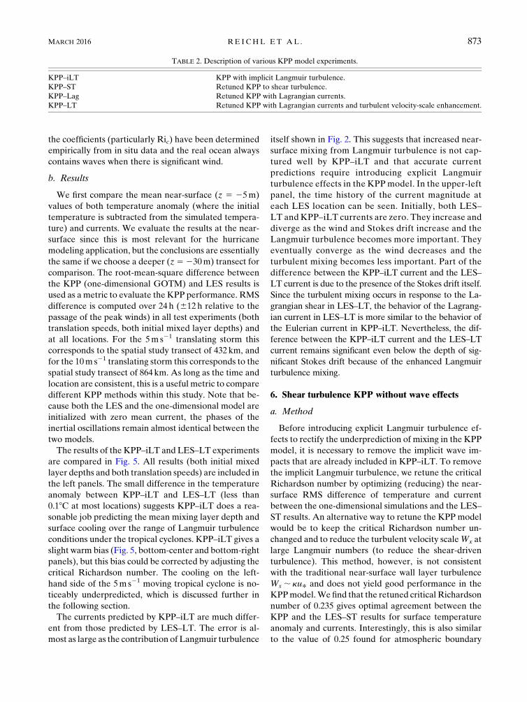
TABLE 2. Description of various KPP model experiments.

KPP–iLT KPP with implicit Langmuir turbulence.

KPP–ST Retuned KPP to shear turbulence.

KPP–Lag Retuned KPP with Lagrangian currents.

KPP–LT Retuned KPP with Lagrangian currents and turbulent velocity-scale enhancement.

MARCH 2016 RE I CHL ET AL . 873

layer closure schemes similar to the KPP (see, e.g., Hong

and Pan 1996). This version of the KPP model is here-

inafter called KPP–ST.

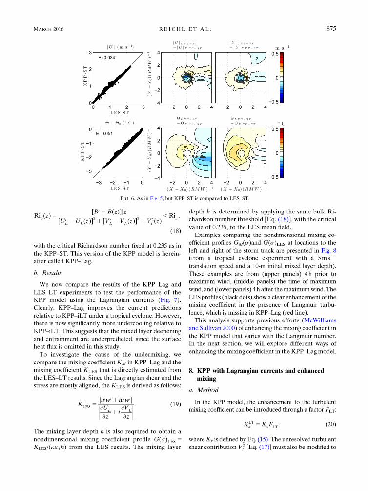
b. Results

The results of the KPP–ST and LES–ST experi-

ments are compared (Fig. 6) in the same manner as

the previous section. The RMS difference for both

near-surface current and temperature anomaly are

considerably reduced across the range of forcing

parameters in this experiment as a result of modify-

ing the critical Richardson number.

As in the case of KPP–iLT (Fig. 5), the cooling on

the left-hand side of the 5m s21 moving tropical cy-

clone is noticeably underpredicted (Fig. 6, lower-

middle panel). This problem is clearly unrelated to

the Langmuir turbulence. It is rather related to KPP’s

shortcoming in handling the rapidly changing wind

forcing. When the wind speed rapidly decreases after

the storm passage, the near-surface current rapidly

decreases as well. The KPPmodel predicts a shallower

mixing layer depth based on the critical Richardson

number criterion, and the deepening of the mixing

layer ceases. However, the LES model shows that the

turbulence near the bottom of the mixing layer does

not weaken as rapidly and the mixing layer continues

to deepen during this phase of the tropical cyclone.

The KPP fails to accurately predict the vertical vari-

ation of the turbulence in such a transient and non-

equilibrium condition. The problem is more evident

on the left-hand side because the mixing layer is much

shallower and the sea surface temperature is more

sensitive to the underprediction of the mixing layer

deepening. Because this is not related to the Langmuir

turbulence effect in the KPP model, we do not address

it any further in this study.

7. KPP with Lagrangian currents

a. Method

Before adding the explicit Langmuir turbulence pa-

rameterization into the KPP–ST model, we consider

the effect of the Lagrangian shear (with the Stokes

drift) in place of the Eulerian shear. Figure 4 indicates a

better alignment between the Reynolds stress and the

Lagrangian shear. In all diffusion equations the current

shear is replaced with the Lagrangian shear as shown in

Eq. (8). In addition, the bulk Richardson number cal-

culation is modified to account for the Lagrangian

(Lag) shear:

FIG. 5. Results of (top) current magnitude and (bottom) temperature anomaly (temperature

minus initial temperature) at 50-m depth. (left) Results from the one-dimensional model with

the KPP–iLT on the vertical axis vs results from the LES–LTmodel on the horizontal axis. The

‘‘E’’ value is theRMSdifference. (center)Difference between results fromKPP–iLT andLES–

LT for the 5m s21 translating tropical cyclone. The horizontal and vertical axes indicate the

distance from the storm center position normalized by the RMW (50 km). (right) As in the

(center), but for the 10m s21 translating tropical cyclone.

874 JOURNAL OF PHYS ICAL OCEANOGRAPHY VOLUME 46

Rib(z)5

[Br 2B(z)]jzj[Ur

L 2UL(z)]2 1 [Vr

L 2VL(z)]2 1V2

t (z),Ri

c,

(18)

with the critical Richardson number fixed at 0.235 as in

the KPP–ST. This version of the KPP model is herein-

after called KPP–Lag.

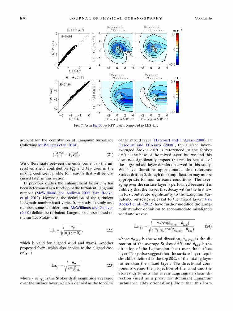
b. Results

We now compare the results of the KPP–Lag and

LES–LT experiments to test the performance of the

KPP model using the Lagrangian currents (Fig. 7).

Clearly, KPP–Lag improves the current predictions

relative to KPP–iLT under a tropical cyclone. However,

there is now significantly more undercooling relative to

KPP–iLT. This suggests that the mixed layer deepening

and entrainment are underpredicted, since the surface

heat flux is omitted in this study.

To investigate the cause of the undermixing, we

compare the mixing coefficient KM in KPP–Lag and the

mixing coefficient KLES that is directly estimated from

the LES–LT results. Since the Lagrangian shear and the

stress are mostly aligned, the KLES is derived as follows:

KLES

5ju0w0 1 iy0w0j����›UL

›z1 i

›VL

›z

����. (19)

The mixing layer depth h is also required to obtain a

nondimensional mixing coefficient profile G(s)LES 5KLES/(ku*h) from the LES results. The mixing layer

depth h is determined by applying the same bulk Ri-

chardson number threshold [Eq. (18)], with the critical

value of 0.235, to the LES mean field.

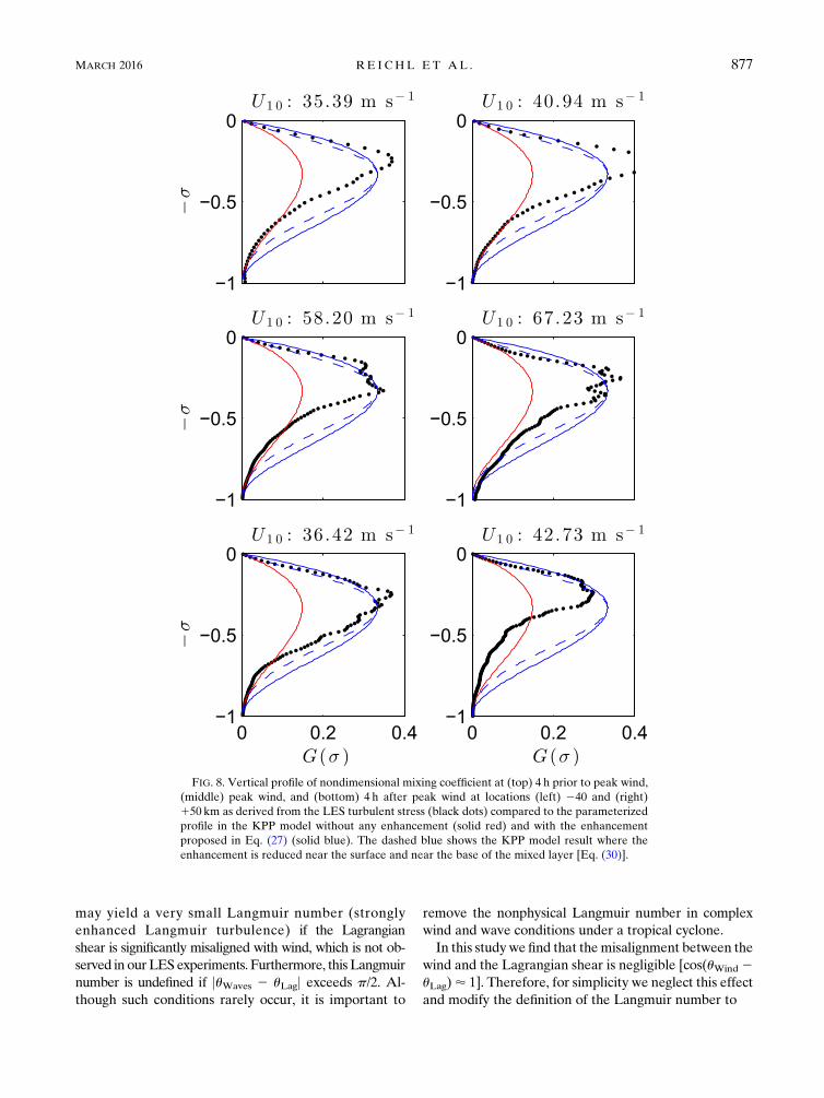
Examples comparing the nondimensional mixing co-

efficient profiles GM(s)and G(s)LES at locations to the

left and right of the storm track are presented in Fig. 8

(from a tropical cyclone experiment with a 5ms21

translation speed and a 10-m initial mixed layer depth).

These examples are from (upper panels) 4h prior to

maximum wind, (middle panels) the time of maximum

wind, and (lower panels) 4h after themaximumwind. The

LESprofiles (black dots) show a clear enhancement of the

mixing coefficient in the presence of Langmuir turbu-

lence, which is missing in KPP–Lag (red line).

This analysis supports previous efforts (McWilliams

and Sullivan 2000) of enhancing themixing coefficient in

the KPP model that varies with the Langmuir number.

In the next section, we will explore different ways of

enhancing themixing coefficient in the KPP–Lagmodel.

8. KPP with Lagrangian currents and enhancedmixing

a. Method

In the KPP model, the enhancement to the turbulent

mixing coefficient can be introduced through a factor FLT:

KLTx 5K

xFLT

, (20)

whereKx is defined byEq. (15). The unresolved turbulent

shear contributionV2t [Eq. (17)] must also be modified to

FIG. 6. As in Fig. 5, but KPP–ST is compared to LES–ST.

MARCH 2016 RE I CHL ET AL . 875

account for the contribution of Langmuir turbulence

(following McWilliams et al. 2014):

(VLTt )2 5V2

t FVtLT . (21)

We differentiate between the enhancement to the un-

resolved shear contribution FVtLT and FLT used in the

mixing coefficient profile for reasons that will be dis-

cussed later in this section.

In previous studies the enhancement factor FLT has

been determined as a function of the turbulent Langmuir

number (McWilliams and Sullivan 2000; Van Roekel

et al. 2012). However, the definition of the turbulent

Langmuir number itself varies from study to study and

requires some consideration. McWilliams and Sullivan

(2000) define the turbulent Langmuir number based on

the surface Stokes drift:

Lat5

ffiffiffiffiffiffiffiffiffiffiffiffiffiffiffiffiffiffiffiffiffiffiu*

juS(z5 0)j

s, (22)

which is valid for aligned wind and waves. Another

proposed form, which also applies to the aligned case

only, is

LaSL

5

ffiffiffiffiffiffiffiffiffiffiffiffiffiffiffiffiu*

hjuSjiSL

s, (23)

where hjuSjiSL is the Stokes drift magnitude averaged

over the surface layer, which is defined as the top 20%

of the mixed layer (Harcourt and D’Asaro 2008). In

Harcourt and D’Asaro (2008), the surface layer–

averaged Stokes drift is referenced to the Stokes

drift at the base of the mixed layer, but we find this

does not significantly impact the results because of

the large mixed layer depths observed in this study.

We have therefore approximated this reference

Stokes drift as 0, though this simplification may not be

appropriate for nonhurricane conditions. The aver-

aging over the surface layer is performed because it is

unlikely that the waves that decay within the first few

meters contribute significantly to the Langmuir tur-

bulence on scales relevant to the mixed layer. Van

Roekel et al. (2012) have further modified the Lang-

muir number definition to accommodate misaligned

wind and waves:

LaSLu

5

ffiffiffiffiffiffiffiffiffiffiffiffiffiffiffiffiffiffiffiffiffiffiffiffiffiffiffiffiffiffiffiffiffiffiffiffiffiffiffiffiffiffiffiffiffiffiffiffiffiffiffiffiu* cos(uWind

2 uLag

)

hjuSjiSL

cos(uWaves

2 uLag

)

vuut , (24)

where uWind is the wind direction, uWaves is the di-

rection of the average Stokes drift, and uLag is the

direction of the Lagrangian shear over the surface

layer. They also suggest that the surface layer depth

should be defined as the top 20% of the mixing layer

rather than the mixed layer. The directional com-

ponents define the projection of the wind and the

Stokes drift into the mean Lagrangian shear di-

rection (used as a proxy for dominant Langmuir

turbulence eddy orientation). Note that this form

FIG. 7. As in Fig. 5, but KPP–Lag is compared to LES–LT.

876 JOURNAL OF PHYS ICAL OCEANOGRAPHY VOLUME 46

may yield a very small Langmuir number (strongly

enhanced Langmuir turbulence) if the Lagrangian

shear is significantly misaligned with wind, which is not ob-

served in ourLES experiments. Furthermore, this Langmuir

number is undefined if juWaves 2 uLagj exceeds p/2. Al-

though such conditions rarely occur, it is important to

remove the nonphysical Langmuir number in complex

wind and wave conditions under a tropical cyclone.

In this studywe find that themisalignment between the

wind and the Lagrangian shear is negligible [cos(uWind 2uLag)’ 1]. Therefore, for simplicity we neglect this effect

and modify the definition of the Langmuir number to

FIG. 8. Vertical profile of nondimensional mixing coefficient at (top) 4 h prior to peak wind,

(middle) peak wind, and (bottom) 4 h after peak wind at locations (left) 240 and (right)

150 km as derived from the LES turbulent stress (black dots) compared to the parameterized

profile in the KPP model without any enhancement (solid red) and with the enhancement

proposed in Eq. (27) (solid blue). The dashed blue shows the KPP model result where the

enhancement is reduced near the surface and near the base of the mixed layer [Eq. (30)].

MARCH 2016 RE I CHL ET AL . 877

LaSLu0 5

ffiffiffiffiffiffiffiffiffiffiffiffiffiffiffiffiffiffiffiffiffiffiffiffiffiffiffiffiffiffiffiffiffiffiffiffiffiffiffiffiffiffiffiffiffiffiffiffiffiffiffiffiffiffiffiffiffiffiffiffiffiffiffiffiffiffiffiffiffiffiffiffiffiffiffiffiu*

hjuSjiSL

1

max[cos(uWaves

2 uLag

), 1028]

s, (25)

that is, the misalignment between the waves, and the La-

grangian shear is limited to p/2 in the Langmuir number

calculation. We also define the surface layer as the top

20% of the mixing layer instead of the mixed layer. Note

that when the misalignment between the waves (Stokes

drift) and the Lagrangian shear exceeds p/2, there is a

possibility that the upper-ocean turbulence is suppressed

instead of enhanced due to surface waves (Rabe et al.

2015), that is, the enhancement factor may become less

than 1. However, we find that such occurrences are rare

(short lived at a particular location) and do not signifi-

cantly affect the mixed layer deepening process. There-

fore, we do not find it necessary to accommodate such

cases in the modified KPP model.

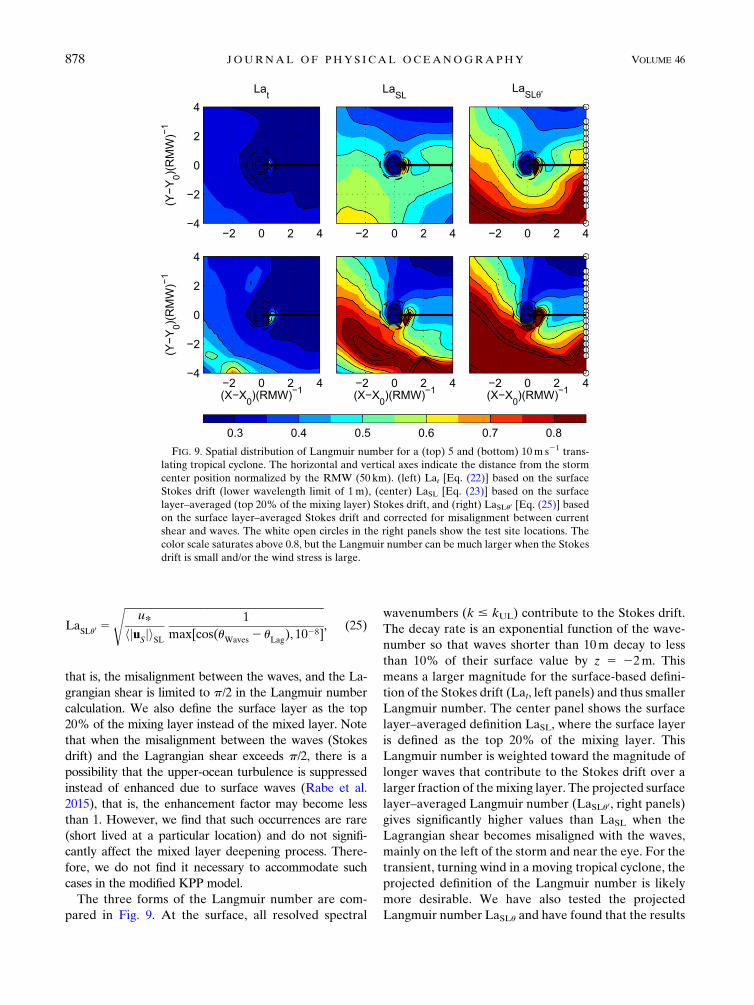
The three forms of the Langmuir number are com-

pared in Fig. 9. At the surface, all resolved spectral

wavenumbers (k # kUL) contribute to the Stokes drift.

The decay rate is an exponential function of the wave-

number so that waves shorter than 10m decay to less

than 10% of their surface value by z 5 22m. This

means a larger magnitude for the surface-based defini-

tion of the Stokes drift (Lat, left panels) and thus smaller

Langmuir number. The center panel shows the surface

layer–averaged definition LaSL, where the surface layer

is defined as the top 20% of the mixing layer. This

Langmuir number is weighted toward the magnitude of

longer waves that contribute to the Stokes drift over a

larger fraction of themixing layer. The projected surface

layer–averaged Langmuir number (LaSLu0, right panels)

gives significantly higher values than LaSL when the

Lagrangian shear becomes misaligned with the waves,

mainly on the left of the storm and near the eye. For the

transient, turning wind in a moving tropical cyclone, the

projected definition of the Langmuir number is likely

more desirable. We have also tested the projected

Langmuir number LaSLu and have found that the results

FIG. 9. Spatial distribution of Langmuir number for a (top) 5 and (bottom) 10m s21 trans-

lating tropical cyclone. The horizontal and vertical axes indicate the distance from the storm

center position normalized by the RMW (50 km). (left) Lat [Eq. (22)] based on the surface

Stokes drift (lower wavelength limit of 1m), (center) LaSL [Eq. (23)] based on the surface

layer–averaged (top 20% of the mixing layer) Stokes drift, and (right) LaSLu0 [Eq. (25)] based

on the surface layer–averaged Stokes drift and corrected for misalignment between current

shear and waves. The white open circles in the right panels show the test site locations. The

color scale saturates above 0.8, but the Langmuir number can be much larger when the Stokes

drift is small and/or the wind stress is large.

878 JOURNAL OF PHYS ICAL OCEANOGRAPHY VOLUME 46

are almost identical to the LaSLu0 except for very small

areas (mainly inside the RMW) where LaSLu0 becomes

extremely small or undefined.

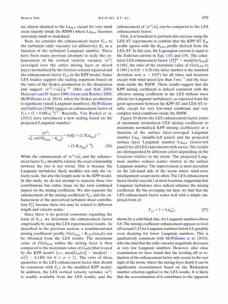
Next, we consider the enhancement factor FLT to

the turbulent eddy viscosity (or diffusivity) Kx as a

function of the turbulent Langmuir number. There

have been many previous attempts to scale the en-

hancement of the vertical velocity variance hw02i(averaged over the entire mixing layer or mixed

layer) normalized by the friction velocity squared and

the enhancement factor FLT in the KPP model. Some

LES studies support the scaling argument based on

the ratio of the Stokes production to the dissipation

and suggest hw02i} u2

*La24/3t (Min and Noh 2004;

Harcourt and D’Asaro 2008; Grant and Belcher 2009;

McWilliams et al. 2014), when the Stokes production

is significant (small Langmuir numbers). McWilliams

and Sullivan (2000) suggest an enhancement factor of

FLT 5 (11 0:08La24t )1/2. Recently, Van Roekel et al.

(2012) have introduced a new scaling based on the

projected Langmuir number:

hw02iu2

*cos2(u

Wind2 u

Lag)5 0:6[11 (1:5La

SLu)22

1 (5:4LaSLu

)24]. (26)

While the enhancement of hw02i/u2

* and the enhance-

ment factor FLT should be related, the exact relationship

between the two is not trivial. This is because the

Langmuir turbulence likely modifies not only the ve-

locity scale, but also the length scale in the KPP model.

In this study, we do not attempt to separate these two

contributions but rather focus on the total combined

impact on the mixing coefficient. We also separate the

enhancement of the mixing coefficient FLT and the en-

hancement of the unresolved turbulent shear contribu-

tion FVtLT because these two may be related to different

length and velocity scales.

Since there is no general consensus regarding the

form of FLT, we determine the enhancement factor

empirically by using the LES experimental results. As

described in the previous section, a nondimensional

mixing coefficient profile G(s)LES 5KLES/(ku*h) can

be obtained from the LES results. The maximum

value of G(s)LES within the mixing layer is then

compared to the maximum value ofGM(s)that is used

by the KPP model fi.e., max[GM(s)] ; max[s(1 2s)2] ; 0.1481 for 0 # s # 1g. The ratio of these

quantities is the LES enhancement factor that should

be consistent with FLT in the modified KPP model.

In addition, the LES vertical velocity variance hw02iis readily available from the LES results, and the

enhancement of hw02i/u2

* can be compared to the LES

enhancement factor.

First, it is beneficial to perform this exercise using the

LES–ST experiments to confirm that the KPP–ST KM

profile agrees with the KLES profile derived from the

LES–ST. In this case, the Lagrangian current is equal to

the Eulerian current in Eqs. (18) and (19). The calcu-

lated LES enhancement factor fFLESLT 5 max[G(s)LES]/

0.1481, the ratio of the maximum value of G(s)LES to

0.1481g is 0.81 6 0.20 (the latter number is the standard

deviation over n 5 6337) for all times and locations

except with wind speed less than 5ms21 and the loca-

tions inside the RMW. These results suggest that the

KPP mixing coefficient is indeed consistent with the

effective mixing coefficient in the LES without wave

effects (no Langmuir turbulence), as expected from the

good agreement between the KPP–ST and LES–ST re-

sults, except for very low-wind conditions and very

complex wind conditions inside the RMW.

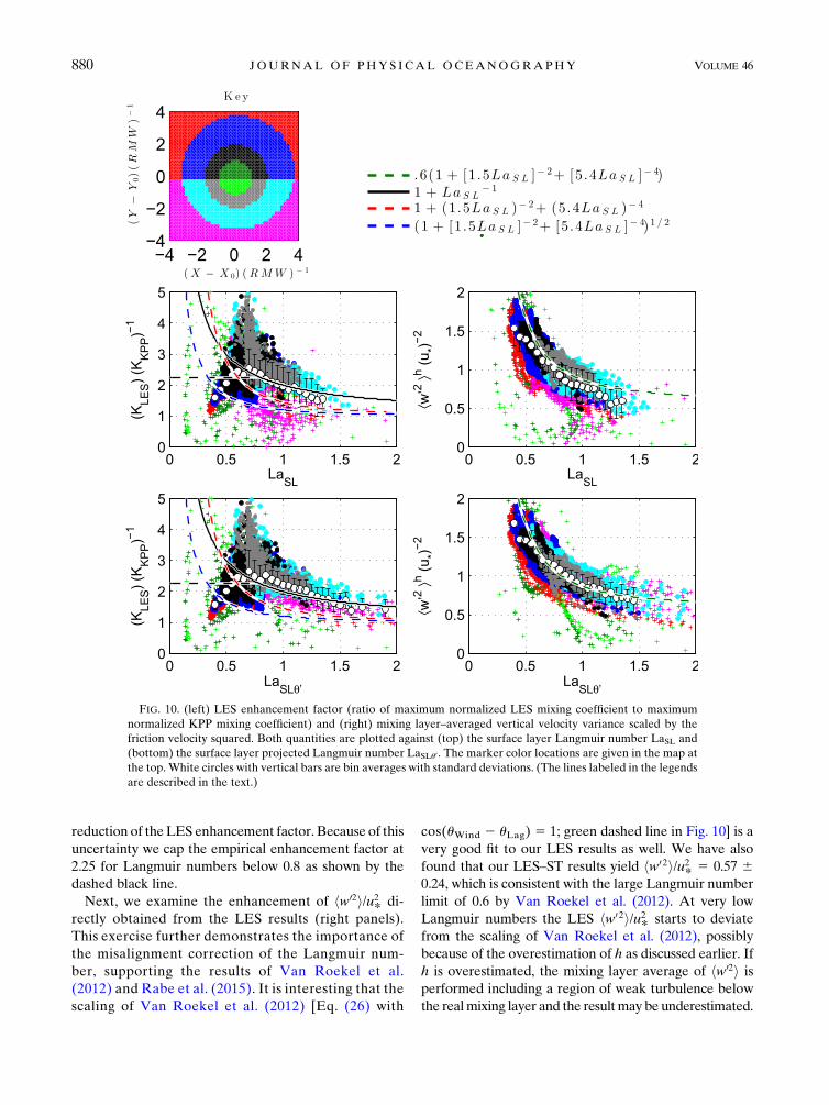
Figure 10 shows the LES enhancement factor (ratio

of maximum normalized LES mixing coefficient to

maximum normalized KPP mixing coefficient) as a

function of the surface layer–averaged Langmuir

number LaSL (middle-left panel) and the projected

surface layer Langmuir number LaSLu0 (lower-left

panel) for all LES experiments with waves. The results

are distinguished by different colors depending on the

locations relative to the storm. The projected Lang-

muir number reduces scatter relative to the surface

Langmuir number. The improvement is most prevalent

on the left-hand side of the storm where wind-wave

misalignment occurs more often. The LES enhancement

factor clearly exceeds 1 atmost locations, suggesting that

Langmuir turbulence does indeed enhance the mixing

coefficient. By bin averaging our data, we find that the

LES enhancement factor scales well with a simple em-

pirical form of

FLT

5 11La21SLu0 , (27)

shown by a solid black line, for Langmuir numbers above

0.8. The mixing coefficient enhancement appears to level

off around 2.25 for Langmuir numbers below 0.8, possibly

even decaying for lower Langmuir numbers. This is

qualitatively consistent with McWilliams et al. (2014),

who also find that the eddy viscositymagnitude decreases

at very low Langmuir numbers. However, after close

examination we have found that the leveling off or re-

duction of the enhancement factor only occurs in the rear

right of the storm, where the mixing layer depth h can be

significantly overestimated based on the Richardson

number criterion applied to the LES results. It is likely

that the overestimation of h contributes to the apparent

MARCH 2016 RE I CHL ET AL . 879

reduction of theLES enhancement factor. Because of this

uncertainty we cap the empirical enhancement factor at

2.25 for Langmuir numbers below 0.8 as shown by the

dashed black line.

Next, we examine the enhancement of hw02i/u2

* di-

rectly obtained from the LES results (right panels).

This exercise further demonstrates the importance of

the misalignment correction of the Langmuir num-

ber, supporting the results of Van Roekel et al.

(2012) and Rabe et al. (2015). It is interesting that the

scaling of Van Roekel et al. (2012) [Eq. (26) with

cos(uWind 2 uLag) 5 1; green dashed line in Fig. 10] is a

very good fit to our LES results as well. We have also

found that our LES–ST results yield hw02i/u2

* 5 0.57 60.24, which is consistent with the large Langmuir number

limit of 0.6 by Van Roekel et al. (2012). At very low

Langmuir numbers the LES hw0 2i/u2

* starts to deviate

from the scaling of Van Roekel et al. (2012), possibly

because of the overestimation of h as discussed earlier. If

h is overestimated, the mixing layer average of hw02i is

performed including a region of weak turbulence below

the realmixing layer and the resultmay be underestimated.

FIG. 10. (left) LES enhancement factor (ratio of maximum normalized LES mixing coefficient to maximum

normalized KPP mixing coefficient) and (right) mixing layer–averaged vertical velocity variance scaled by the

friction velocity squared. Both quantities are plotted against (top) the surface layer Langmuir number LaSL and

(bottom) the surface layer projected Langmuir number LaSLu0. The marker color locations are given in the map at

the top. White circles with vertical bars are bin averages with standard deviations. (The lines labeled in the legends

are described in the text.)

880 JOURNAL OF PHYS ICAL OCEANOGRAPHY VOLUME 46

We do not compare our results with the enhancement

factor given by McWilliams and Sullivan (2000) since

their form was obtained using the very different

Langmuir number Lat based on the surface Stokes

drift. The scaling of hw02i/u2

* presented in Harcourt

and D’Asaro (2008) avoids the asymptotic breakdown

as La / 0 (see McWilliams and Sullivan 2000;

Harcourt and D’Asaro 2008), unlike the scaling of

Van Roekel et al. (2012). However, the difference

between these two is appreciable only at very low

Langmuir numbers where our results are not reliable.

We also note that the values of hw02i can be quite

different if the averaging is done over the entire mixed

layer (Van Roekel et al. 2012; Rabe et al. 2015) in-

stead of the entire mixing layer (this study).

We now investigate the relationship between the

LES enhancement factor and the enhancement of

hw02i/u2

*. If we assume that the length scale of the

KPP mixing coefficient KM is not affected by the

Langmuir turbulence and the velocity scale of KM is

enhanced in the same manner as the square root of

the vertical velocity variance hw02i, the enhancement

factor FLT should be identical to the square root of

hw02i/u2

* divided by its limiting value at large Lang-

muir numbers (no Langmuir turbulence). Then, the

scaling by Van Roekel et al. (2012) [Eq. (26)] sug-

gests that

FLT

5 [11 (1:5LaSLu

)22 1 (5:4LaSLu

)24]1/2. (28)

However, this scaling significantly underestimates the

LES enhancement factor (blue dashed line in the left

panels of Fig. 10). If we instead assume that FLT is iden-

tical to the enhancement to hw02i/u2

*, the scaling of Van

Roekel et al. (2012) suggests

FLT

5 11 (1:5LaSLu

)22 1 (5:4LaSLu

)24. (29)

This scaling (red dashed line in the left panels) is more

consistent in terms of the order of magnitude but still

underestimates the LES enhancement factors except for

very low Langmuir numbers. These exercises suggest

that the enhancement to the velocity and length scales of

KM is not simply related to the enhancement of the

vertical velocity variance hw02i and support our ap-

proach of determining FLT empirically.

The ratio of KM andKLES is not constant with depth

(see Fig. 8). Comparing many similar profiles, we find

that this ratio roughly peaks at the maximum of the

KM profile and approaches 1 at the top and bottom

boundaries. For that reason we apply the enhancement

factor at its maximum where the nondimensional profile

also reaches its maximum. The enhancement factor is

then reduced to 1 approaching both the top and bottom

boundaries.

In summary, based on this analysis, we set our KPP

Langmuir turbulence enhancement factor FKLT as

FKLT(s)5 11 (F 0

LT 2 1)Gx(s)/max[G

x(s)] , (30)

F 0LT 5 11La21

SLu0 , LaSLu0 $ 0:8, (31)

(black solid line in Fig. 10) and

F 0LT 5 2:25, La

SLu0 # 0:8, (32)

(black dashed line in Fig. 10). Referring back to Fig. 8,

the KPP profile with the enhancement (blue) clearly

does a better job reproducing the LES turbulent mixing

coefficient profile compared to the KPP profile without

the enhancement (red). The impact of reducing the en-

hancement toward the bottom and the top (blue dashed)

greatly improves agreement near the surface and helps

avoid overentrainment of cool water at the base of the

mixing layer.

We find that using the same form of the enhancement

factor in both the turbulent mixing profile Kx and the

unresolved shear Vt does not work. This supports the

conclusion of McWilliams et al. (2014) that the scale of

Langmuir turbulence that contributes to the near-

surface mixing is different from the scale of Langmuir

turbulence that drives mixed layer deepening. The

deepening of the mixing layer (the contribution of

Langmuir turbulence to theVt term) is underpredicted if

the same enhancement factor [Eqs. (31) and (32)] is

used. To address this, we empirically modify the en-

hancement factor for Vt to

FVtLT 5 11 2:3La21/2

SLu0 (33)

so that the bulk Richardson number calculation is now

Rib(z)5

[Br 2B(z)]jzj[Ur

L 2UL(z)]2 1 [Vr

L 2VL(z)]2 1 [V

t(z)FVt

LT]2.

(34)

This form [Eq. (33)] was found by optimizing the

agreement between the one-dimensional model and

the LES results of mixing layer depth evolution and

surface cooling, by varying both the slope and mag-

nitude of the enhancement factor while maintaining

that the enhancement factor approaches one in the

large Langmuir number limit.

The KPPmodel with the Lagrangian shear (instead of

the Eulerian shear) and with the enhancement factors,

in the form of Eqs. (30)–(32) forKx andEq. (33) forVt, is

hereinafter called KPP–LT.

MARCH 2016 RE I CHL ET AL . 881

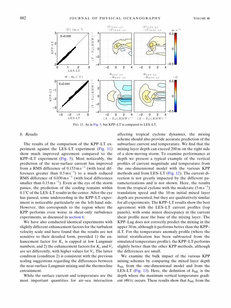
b. Results

The results of the comparison of the KPP–LT ex-

periment against the LES–LT experiment (Fig. 11)

show much improved agreement compared to the

KPP–iLT experiment (Fig. 5). Most noticeably, the

prediction of the near-surface current has improved

from a RMS difference of 0.153m s21 (with local dif-

ferences greater than 0.5m s21) to a much reduced

RMS difference of 0.030m s21 (with local differences

smaller than 0.15m s21). Even as the eye of the storm

passes, the prediction of the cooling remains within

0.18C of the LES–LT results in the center. After the eye

has passed, some undercooling in the KPP–LT exper-

iment is noticeable particularly on the left-hand side.

However, this corresponds to the region where the

KPP performs even worse in shear-only turbulence

experiments, as discussed in section 6.

We have also conducted identical experiments with

slightly different enhancement factors for the turbulent

velocity scale and have found that the results are not

sensitive to their detailed form, provided 1) the en-

hancement factor for Kx is capped at low Langmuir

numbers, and 2) the enhancement factors for Kx and Vt

are set differently, with higher values for Vt. The latter

condition (condition 2) is consistent with the previous

scaling suggestions regarding the differences between

the near-surface Langmuir mixing and the thermocline

entrainment.

While the surface current and temperature are the

most important quantities for air–sea interaction

affecting tropical cyclone dynamics, the mixing

scheme should also provide accurate prediction of the

subsurface current and temperature. We find that the

mixing layer depth can exceed 200m on the right side

of a slow-moving storm. To examine performance at

depth we present a typical example of the vertical

profiles of current magnitude and temperature from

the one-dimensional model with the various KPP

methods and from LES–LT (Fig. 12). The current di-

rection is not greatly impacted by the different pa-

rameterizations and is not shown. Here, the results

from the tropical cyclone with the moderate (5m s21)

translation speed and the 10-m initial mixed layer

depth are presented, but they are qualitatively similar

for all experiments. The KPP–LT results show the best

agreement with the LES–LT current profiles (top

panels), with some minor discrepancy in the current

shear profile near the base of the mixing layer. The

KPP–Lag does not correctly predict the mixing in the

upper 30m, although it performs better than the KPP–

iLT. For the temperature anomaly profile (where the

initial stratification has been subtracted from the

simulated temperature profile), the KPP–LT performs

slightly better than the other KPP methods, although

the differences are small.

We examine the bulk impact of the various KPP

mixing schemes by comparing the mixed layer depth

hML from the one-dimensional model and from the

LES–LT (Fig. 13). Here, the definition of hML is the

depth where the maximum vertical temperature gradi-

ent ›Q/›z occurs. These results show that hML from the

FIG. 11. As in Fig. 5, but KPP–LT is compared to LES–LT.

882 JOURNAL OF PHYS ICAL OCEANOGRAPHY VOLUME 46

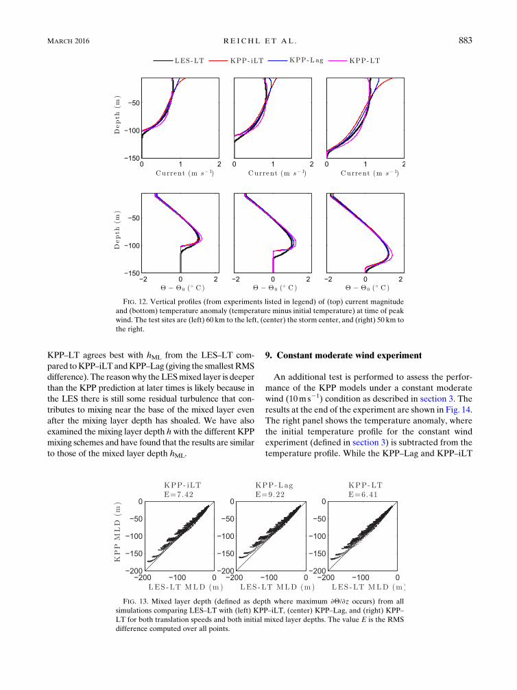
KPP–LT agrees best with hML from the LES–LT com-

pared toKPP–iLTandKPP–Lag (giving the smallestRMS

difference). The reasonwhy theLESmixed layer is deeper

than the KPP prediction at later times is likely because in

the LES there is still some residual turbulence that con-

tributes to mixing near the base of the mixed layer even

after the mixing layer depth has shoaled. We have also

examined the mixing layer depth hwith the different KPP

mixing schemes and have found that the results are similar

to those of the mixed layer depth hML.

9. Constant moderate wind experiment

An additional test is performed to assess the perfor-

mance of the KPP models under a constant moderate

wind (10ms21) condition as described in section 3. The

results at the end of the experiment are shown in Fig. 14.

The right panel shows the temperature anomaly, where

the initial temperature profile for the constant wind

experiment (defined in section 3) is subtracted from the

temperature profile. While the KPP–Lag and KPP–iLT

FIG. 12. Vertical profiles (from experiments listed in legend) of (top) current magnitude

and (bottom) temperature anomaly (temperature minus initial temperature) at time of peak

wind. The test sites are (left) 60 km to the left, (center) the storm center, and (right) 50 km to

the right.

FIG. 13. Mixed layer depth (defined as depth where maximum ›Q/›z occurs) from all

simulations comparing LES–LT with (left) KPP–iLT, (center) KPP–Lag, and (right) KPP–

LT for both translation speeds and both initial mixed layer depths. The value E is the RMS

difference computed over all points.

MARCH 2016 RE I CHL ET AL . 883

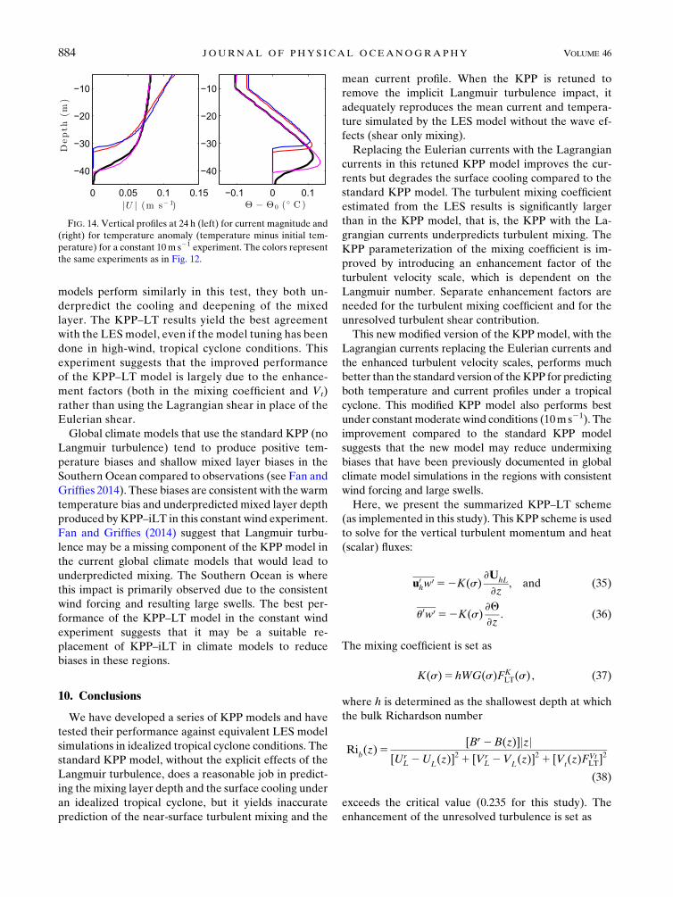
models perform similarly in this test, they both un-

derpredict the cooling and deepening of the mixed

layer. The KPP–LT results yield the best agreement

with the LESmodel, even if the model tuning has been

done in high-wind, tropical cyclone conditions. This

experiment suggests that the improved performance

of the KPP–LT model is largely due to the enhance-

ment factors (both in the mixing coefficient and Vt)

rather than using the Lagrangian shear in place of the

Eulerian shear.

Global climate models that use the standard KPP (no

Langmuir turbulence) tend to produce positive tem-

perature biases and shallow mixed layer biases in the

Southern Ocean compared to observations (see Fan and

Griffies 2014). These biases are consistent with the warm

temperature bias and underpredicted mixed layer depth

produced by KPP–iLT in this constant wind experiment.

Fan and Griffies (2014) suggest that Langmuir turbu-

lence may be a missing component of the KPP model in

the current global climate models that would lead to

underpredicted mixing. The Southern Ocean is where

this impact is primarily observed due to the consistent

wind forcing and resulting large swells. The best per-

formance of the KPP–LT model in the constant wind

experiment suggests that it may be a suitable re-

placement of KPP–iLT in climate models to reduce

biases in these regions.

10. Conclusions

We have developed a series of KPP models and have

tested their performance against equivalent LES model

simulations in idealized tropical cyclone conditions. The

standard KPP model, without the explicit effects of the

Langmuir turbulence, does a reasonable job in predict-

ing the mixing layer depth and the surface cooling under

an idealized tropical cyclone, but it yields inaccurate

prediction of the near-surface turbulent mixing and the

mean current profile. When the KPP is retuned to

remove the implicit Langmuir turbulence impact, it

adequately reproduces the mean current and tempera-

ture simulated by the LES model without the wave ef-

fects (shear only mixing).

Replacing the Eulerian currents with the Lagrangian

currents in this retuned KPP model improves the cur-

rents but degrades the surface cooling compared to the

standard KPP model. The turbulent mixing coefficient

estimated from the LES results is significantly larger

than in the KPP model, that is, the KPP with the La-

grangian currents underpredicts turbulent mixing. The

KPP parameterization of the mixing coefficient is im-

proved by introducing an enhancement factor of the

turbulent velocity scale, which is dependent on the

Langmuir number. Separate enhancement factors are

needed for the turbulent mixing coefficient and for the

unresolved turbulent shear contribution.

This new modified version of the KPP model, with the

Lagrangian currents replacing the Eulerian currents and

the enhanced turbulent velocity scales, performs much

better than the standard version of theKPP for predicting

both temperature and current profiles under a tropical

cyclone. This modified KPP model also performs best

under constant moderate wind conditions (10ms21). The

improvement compared to the standard KPP model

suggests that the new model may reduce undermixing

biases that have been previously documented in global

climate model simulations in the regions with consistent

wind forcing and large swells.

Here, we present the summarized KPP–LT scheme

(as implemented in this study). This KPP scheme is used

to solve for the vertical turbulent momentum and heat

(scalar) fluxes:

u0hw

0 52K(s)›U

hL

›z, and (35)

u0w0 52K(s)›Q

›z. (36)

The mixing coefficient is set as

K(s)5 hWG(s)FKLT(s) , (37)

where h is determined as the shallowest depth at which

the bulk Richardson number

Rib(z)5

[Br 2B(z)]jzj[Ur

L 2UL(z)]2 1 [Vr

L 2VL(z)]2 1 [V

t(z)FVt

LT]2

(38)

exceeds the critical value (0.235 for this study). The

enhancement of the unresolved turbulence is set as

FIG. 14. Vertical profiles at 24 h (left) for current magnitude and

(right) for temperature anomaly (temperature minus initial tem-

perature) for a constant 10m s21 experiment. The colors represent

the same experiments as in Fig. 12.

884 JOURNAL OF PHYS ICAL OCEANOGRAPHY VOLUME 46

FVtLT 5 11 2:3La21/2

SLu0 , (39)

and the enhancement to the turbulent mixing coefficient

is set as

FKLT(s)5 11 (F 0

LT 2 1)G(s)/max[G(s)] , (40)

F 0LT 5 11La21

SLu0 , LaSLu0 $ 0:8, and (41)

F 0LT 5 2:25, La

SLu0 # 0:8. (42)

The next step of this research will be to introduce this

modified KPP model into three-dimensional ocean

models. This will allow the impact of the Langmuir

turbulence to be more thoroughly evaluated against

available in situ observations.

Acknowledgments. The authors acknowledge NSF

Grants OCE1129985(URI) and OCE1130678(UD) for

funding this work. We acknowledge Dr. Peter Sullivan

(NCAR) for providing the original LES code used in this

study. We also acknowledge high-performance com-

puting support from Information Technologies (IT) re-

sources at the University of Delaware and Yellowstone

(ark:/85065/d7wd3xhc) provided by NCAR’s Compu-

tational and Information Systems Laboratory, spon-

sored by the National Science Foundation. We thank

the anonymous reviewers whose helpful suggestions

contributed to improving the content and presentation

of this manuscript.

REFERENCES

Craig, P. D., and M. L. Banner, 1994: Modeling wave-enhanced

turbulence in the ocean surface layer. J. Phys. Oceanogr.,

24, 2546–2559, doi:10.1175/1520-0485(1994)024,2546:

MWETIT.2.0.CO;2.

Craik, A. D. D., and S. Leibovich, 1976: A rational model for

Langmuir circulations. J. Fluid Mech., 73, 401–426, doi:10.1017/

S0022112076001420.

D’Alessio, J. S. D., K. Abdella, and N. A. McFarlane, 1998: A new

second-order turbulence closure scheme for modeling the

oceanic mixed layer. J. Phys. Oceanogr., 28, 1624–1641,

doi:10.1175/1520-0485(1998)028,1624:ANSOTC.2.0.CO;2.

D’Asaro, E., J. Thomson, A. Shcherbina, R. Harcourt, M. Cronin,

M. Hemer, and B. Fox-Kemper, 2014: Quantifying upper

ocean turbulence driven by surfacewaves.Geophys. Res. Lett.,

41, 102–107, doi:10.1002/2013GL058193.

Emanuel, K. A., 1991: The theory of hurricanes. Annu. Rev. Fluid

Mech., 23, 179–196, doi:10.1146/annurev.fl.23.010191.001143.——, 1999: Thermodynamic control of hurricane intensity.Nature,

401, 665–669, doi:10.1038/44326.

Fan, Y., and S. M. Griffies, 2014: Impacts of parameterized Lang-

muir turbulence and nonbreaking wave mixing in global cli-

mate simulations. J. Climate, 27, 4752–4775, doi:10.1175/

JCLI-D-13-00583.1.

——, I. Ginis, T. Hara, C. W. Wright, and E. J. Walsh, 2009: Nu-

merical simulations and observations of surface wave fields

under an extreme tropical cyclone. J. Phys. Oceanogr., 39,

2097–2116, doi:10.1175/2009JPO4224.1.

Ginis, I., 2002: Tropical cyclone–ocean interactions. Atmosphere–

Ocean Interactions, Volume 1, W. Perrie, Ed., Advances in

Fluid Mechanics Series, No. 22, WIT Press, 83–114.

Grant, A. L. M., and S. E. Belcher, 2009: Characteristics of Lang-

muir turbulence in the ocean mixed layer. J. Phys. Oceanogr.,

39, 1871–1887, doi:10.1175/2009JPO4119.1.

Griffies, S. M., M. Levy, A. J. Adcroft, G. Danabasoglu,

D. Jacobsen, W. Large, and T. Ringler, 2013: Theory and

numerics of the CommunityOcean VerticalMixing (CVMIX)

project. Tech. Rep., 94 pp. [Available online at https://

cvmix.googlecode.com/svn/trunk/manual/cvmix.pdf.]

Harcourt, R. R., 2013: A second-moment closure model of Lang-

muir turbulence. J. Phys. Oceanogr., 43, 673–697, doi:10.1175/

JPO-D-12-0105.1.

——, 2015: An improved second-moment closure model of Lang-

muir turbulence. J. Phys. Oceanogr., 45, 84–103, doi:10.1175/

JPO-D-14-0046.1.

——, andE.A.D’Asaro, 2008: Large-eddy simulation of Langmuir

turbulence in pure wind seas. J. Phys. Oceanogr., 38, 1542–

1562, doi:10.1175/2007JPO3842.1.

Holland, G. J., 1980: An analytic model of the wind and

pressure profiles in hurricanes. Mon. Wea. Rev.,

108, 1212–1218, doi:10.1175/1520-0493(1980)108,1212:

AAMOTW.2.0.CO;2.

Hong, S.-Y., and H.-L. Pan, 1996: Nonlocal boundary layer vertical

diffusion in a medium-range forecast model. Mon. Wea. Rev.,

124, 2322–2339, doi:10.1175/1520-0493(1996)124,2322:

NBLVDI.2.0.CO;2.

Kantha, L. H., and C. A. Clayson, 2004: On the effect of surface

gravity waves on mixing in the oceanic mixed layer. Ocean

Modell., 6, 101–124, doi:10.1016/S1463-5003(02)00062-8.

Kukulka, T., A. J. Plueddemann, J. H. Trowbridge, and P. P.

Sullivan, 2009: Significance of Langmuir circulation in

upper ocean mixing: Comparison of observations and

simulations. Geophys. Res. Lett., 36, L10603, doi:10.1029/

2009GL037620.

——, ——, ——, and ——, 2010: Rapid mixed layer deepening

by the combination of Langmuir and shear instabilities: A

case study. J. Phys. Oceanogr., 40, 2381–2400, doi:10.1175/

2010JPO4403.1.

Langmuir, I., 1938: Surface motion of water induced by wind.

Science, 87, 119–123, doi:10.1126/science.87.2250.119.

Large, W. G., J. C. McWilliams, and S. C. Doney, 1994: Oceanic

vertical mixing: A review and a model with a nonlocal boundary

layer parameterization. Rev. Geophys., 32, 363–403, doi:10.1029/

94RG01872.

McWilliams, J. C., and J.M. Restrepo, 1999: The wave-driven ocean

circulation. J. Phys. Oceanogr., 29, 2523–2540, doi:10.1175/

1520-0485(1999)029,2523:TWDOC.2.0.CO;2.

——, and P. P. Sullivan, 2000: Vertical mixing by Langmuir cir-

culations. Spill Sci. Technol. Bull., 6, 225–237, doi:10.1016/

S1353-2561(01)00041-X.

——, ——, and C.-H. Moeng, 1997: Langmuir turbulence in

the ocean. J. Fluid Mech., 334, 1–30, doi:10.1017/

S0022112096004375.

——, E. Huckle, J.-H. Liang, and P. P. Sullivan, 2012: The wavy

Ekman layer: Langmuir circulations, breaking waves, and

Reynolds stress. J. Phys. Oceanogr., 42, 1793–1816, doi:10.1175/

JPO-D-12-07.1.

——, ——, ——, and ——, 2014: Langmuir turbulence in swell.

J. Phys.Oceanogr., 44, 870–890, doi:10.1175/JPO-D-13-0122.1.

MARCH 2016 RE I CHL ET AL . 885

Mellor, G. L., and T. Yamada, 1982: Development of a turbulence

closure model for geophysical fluid problems. Rev. Geophys.

Space Phys., 20, 851–875, doi:10.1029/RG020i004p00851.

Melville, W. K., 1996: The role of surface-wave breaking in air-sea

interaction.Annu. Rev. Fluid Mech., 28, 279–321, doi:10.1146/

annurev.fl.28.010196.001431.

Min, H. S., and Y. Noh, 2004: Influence of the surface heating on

Langmuir circulation. J. Phys. Oceanogr., 34, 2630–2641,

doi:10.1175/JPOJPO-2654.1.

Moon, I.-J., I. Ginis, T. Hara, H. L. Tolman, C.W.Wright, and E. J.

Walsh, 2003: Numerical simulation of sea surface directional

wave spectra under hurricane wind forcing. J. Phys. Ocean-

ogr., 33, 1680–1706, doi:10.1175/2410.1.

Noh, Y., H. S.Min, and S. Raasch, 2004: Large eddy simulation of the

ocean mixed layer: The effects of wave breaking and Langmuir

circulation. J. Phys. Oceanogr., 34, 720–735, doi:10.1175/

1520-0485(2004)034,0720:LESOTO.2.0.CO;2.

——, G. Goh, and S. Raasch, 2011: Influence of Langmuir circu-

lation on the deepening of the wind-mixed layer. J. Phys.

Oceanogr., 41, 472–484, doi:10.1175/2010JPO4494.1.

Polton, J. A., and S. E. Belcher, 2007: Langmuir turbulence and

deeply penetrating jets in an unstratifiedmixed layer. J.Geophys.

Res., 112, C09020, doi:10.1029/2007JC004205.Price, J. F., 1981: Upper ocean response to a hurricane. J. Phys.

Oceanogr., 11, 153–175, doi:10.1175/1520-0485(1981)011,0153:

UORTAH.2.0.CO;2.

Rabe, T. J., T. Kukulka, I. Ginis, T. Hara, B. G. Reichl, E. A.

D’Asaro, R. R. Harcourt, and P. P. Sullivan, 2015: Langmuir

turbulence under Hurricane Gustav (2008). J. Phys. Ocean-

ogr., 45, 657–677, doi:10.1175/JPO-D-14-0030.1.

Sanford, T. B., J. F. Price, and J. B. Girton, 2011: Upper-ocean re-

sponse to Hurricane Frances (2004) observed by profiling

EM-APEXfloats. J. Phys. Oceanogr., 41, 1041–1056, doi:10.1175/

2010JPO4313.1.

Sinha, N., A. E. Tejada-Martinez, C. Akan, and C. E. Grosch, 2015:

Toward a K-profile parameterization of Langmuir turbulence

in shallow coastal shelves. J. Phys. Oceanography, 45, 2869–2895, doi:10.1175/JPO-D-14-0158.1.

Skyllingstad, E. D., and D. W. Denbo, 1995: An ocean large-eddy

simulation of Langmuir circulations and convection in the

surface mixed layer. J. Geophys. Res., 100, 8501–8522,

doi:10.1029/94JC03202.

——, W. D. Smyth, and G. B. Crawford, 2000: Resonant wind-

drivenmixing in the ocean boundary layer. J. Phys. Oceanogr.,

30, 1866–1890, doi:10.1175/1520-0485(2000)030,1866:

RWDMIT.2.0.CO;2.

Smyth, W. D., E. D. Skyllingstad, G. B. Crawford, and

H.Wijesekera, 2002: Nonlocal fluxes and Stokes drift effects in

the K-profile parameterization. Ocean Dyn., 52, 104–115,

doi:10.1007/s10236-002-0012-9.

Sullivan, P. P., J. C. McWilliams, and W. K. Melville, 2007:

Surface gravity wave effects in the oceanic boundary layer:

Large-eddy simulation with vortex force and stochastic

breakers. J. Fluid Mech., 593, 405–452, doi:10.1017/

S002211200700897X.

——, L. Romero, J. C. McWilliams, and W. K. Melville, 2012:

Transient evolution of Langmuir turbulence in ocean bound-

ary layers driven by hurricane winds and waves. J. Phys.

Oceanogr., 42, 1959–1980, doi:10.1175/JPO-D-12-025.1.

Teixeira, M. A. C., and S. E. Belcher, 2010: On the structure of

Langmuir turbulence. Ocean Modell., 31, 105–119, doi:10.1016/

j.ocemod.2009.10.007.

Terray, E. A., M. A. Donelan, Y. C. Agrawal, W. M. Drennan, K. K.

Kahma,A. J.Williams III, P.A.Hwang, and S.A.Kitaigorodskii,

1996: Estimates of kinetic energy dissipation under break-

ing waves. J. Phys. Oceanogr., 26, 792–807, doi:10.1175/

1520-0485(1996)026,0792:EOKEDU.2.0.CO;2.

Tolman, H. L., 2009: User manual and system documentation of

WAVEWATCH III version 3.14. NOAA/NWS/NCEP/EMC/

MMAB Tech. Note 276, 220 pp.

Umlauf, L., H. Burchard, and K. Bolding, 2005: GOTM: Scientific

documentation. 3rd ed. Leiniz-Institute for Baltic Sea Re-

search Marine Science, 360 pp. [Available online at http://

www.gotm.net/pages/documentation/manual/stable/pdf/a4.pdf.]

Van Roekel, L. P., B. Fox-Kemper, P. P. Sullivan, P. E.

Hamlington, and S. R. Haney, 2012: The form and orientation

of Langmuir cells for misalinged winds and waves. J. Geophys.

Res., 117, C05001, doi:10.1029/2011JC007516.Yablonsky, R. M., and I. Ginis, 2009: Limitation of one-

dimensional ocean models for coupled hurricane–ocean

model forecasts. Mon. Wea. Rev., 137, 4410–4419, doi:10.1175/2009MWR2863.1.

Young, I. R., 2003: A review of the sea state generated

by hurricanes. Mar. Struct., 16, 201–218, doi:10.1016/

S0951-8339(02)00054-0.

Zhang, J. A., and E. W. Uhlhorn, 2012: Hurricane sea surface in-

flow angle and an observation-based parametric model. Mon.

Wea. Rev., 140, 3587–3605, doi:10.1175/MWR-D-11-00339.1.

886 JOURNAL OF PHYS ICAL OCEANOGRAPHY VOLUME 46