land misallocation and productivity - imf · land misallocation and productivity diego restuccia...

Land Misallocation and Productivity

Diego RestucciaUniversity of Toronto

Raul Santaeulalia-LlopisWashington University in St. Louis

Workshop on Macroeconomic Policy and InequalityWashington – Sep. 18-19, 2014

1/62

Motivation

I Why are some countries richer than others?

I Many useful perspectives. We focus on two dimensions:

(a) Agriculture is important in accounting for productivitydifferences across countries:

I poor are much less productive in agriculture than innon-agriculture relative to rich countries

I low productivity in agriculture means more people inagriculture to satisfy subsistence consumption

I Challenge: why are poor countries so much less productivein agriculture?...

(b) Misallocation of factors across heterogeneous productionunits have a role explaining productivity levels.

2/62

I We argue that land (mis)allocation is important foragricultural productivity.

I We focus on Malawi. Why?I Land markets are restricted and underdeveloped: Most

land is either inherited (73%) or granted by local chiefs11.9%). Only 1.1% of land is purchased (with a title) andonly 6.9% is rented.

I We have detailed representative household-farm data toidentify farm-level productivity.

3/62

What We Do and Find

1. We estimate farm-level productivity using unique micro datafrom household-farms in Malawi. From very detailed data onfarm output and inputs:

I We capture the full degree of heterogeneity in land quality & rain(unanticipated output shocks).

I Development accounting: Negligible role of quality & rain.

2. We estimate extent of factor misallocation: yield and capitalproductivity are strongly positively related to productivity,providing empirical evidence of misallocation.

3. We assess the impact of misallocation for agriculturalproductivity with a simple efficient framework:

I Counterfactual: If land is efficiently reallocated agriculturalproductivity increases by 3 times its value.

I Our result is robust to within narrow definitions ofgeographical areas, traditional authority, language, humancapital.

4/62

The Micro Data: Malawi ISA 2010

I New and unique nationally-representative household data,World Bank (see de Magalhaes and Santaeulalia-Llopis, 2014).

I The original sample includes 12,271 households of which about81% live in rural areas.

I The survey follows a stratified 2-stage sample design.1. 768 enumeration areas (EAs) were selected with PPS within each district.2. Random systematic sampling was used to select 16 primary households

and 5 replacement households from the household listing for each EA.

I Very detailed information on inputs and outputs makes thisdataset ideal for our exercise.

I Sample is rolled over 12 months from March 2010 to March2011. Sesonality is accurately addressed.

5/62

The Micro Data: Malawi 2010 ISA: A Snapshot

I Agricultural Production: 70% of all income in rural Malawi. Rainyseason 93% of total crop. Maize represents 78% of total production.Resolve issues of physical units conversion to estimate the unsoldproduction.

I Land: Info on each cultivated household plot (owned plus rented-in).Average plots per household-farm are 1.8. Size accurately measuredvia GPS. The sum of all operated plots is land size.

I Capital: Full array of capital types. Equipment: includes implements(hand hoe, etc.) and machinery. Structures: includes chicken houses,livestock kraals... etc. We use the selling price.

I Hours: Most households members work in the field (size=4.57).Individual info on extensive and intensive margins of labor supply: (i)weeks worked, (ii) days/week, and (iii) hours/day by plot & byagricultural activity:

I land preparation/ planting,I weeding/fertilizing, andI harvesting and by season (rainy, dry and permanent).

Measurement Error

6/62

Some Facts

7/62

Fact 1: Small Farm Operational Scale

Percentage of Farms by Size Class

Hectares Malawi (cum) Belgium (cum) USA≤ 1 Ha 77.7 14.6 –1−2 Ha 17.3 8.5 –2−5 Ha 5.0 (100) 15.5 (38.6) 10.65−10 Ha 0.0 14.8 7.510+ Ha 0.0 46.6 81.9

Average Farm Size (Ha) 0.7 16.1 187.0

Notes:Data for Belgium and USA from the 1990 Census.

I In acres, 40% of Malawi’s farmers have <1, 73%<2, 90<3, 95%<4.

I Variance of logs is .618, 90/10 is 7.67, 75/25 is 2.78, Gini .50.

8/62

Fact 2: Most production used for ownconsumption

I Food insecurity last 12 m is on average 50.6% (top 10% of agri.production face 28%, bottom 10% face 80.7%). High foodconsumption/ag. production. 67% of all consumption is food.

Fact 3: Farms use land at (almost) full capacityI We include owned plots, and rented-in plots. There are 283 rural

households without plots. The total share of land that is notcultivated is: less than 3%. Some left fallow.

9/62

Fact 4. Evidence by Farm Productivity

I Fact 4.1: Land does not increase with farm productivity(uncorrelated)

I Fact 4.2: Capital does not increase with farm productivity(uncorrelated)

I Fact 4.3: Capital-land ratio is roughly constant across farmproductivity.

I Fact 4.4: Yield (output per unit of land) increases with farmproductivity.

I Fact 4.5: Capital productivity (output per unit of capital) isincreases with farm productivity.

10/62

Estimating Farm Productivity

We identify household farm productivity si as the unobservablesi in

yi = siζikθki (qi li)

θl

where θx are input factor shares.

I ζi represents unanticipated shocks (e.g. rain), and

I qi is an index of land quality.

11/62

Land Quality Dimensions

VERY detailed information on the land quality per plot (andhousehold). We use full set of 11 dimensions reported in ISA.

1. Elevation2. Slope3. Erosion4. Soil Quality5. Nutrient Availability6. Nutrient Retention Capacity7. Rooting Conditions8. Oxygen Availability to Roots9. Excess Salts

10. Toxicity11. Workability

12/62

Land Quality Dimensions (continued)

Farm heterogeneity in terrain roughness (elevation and slope):

RegionsFull Sample North Center South

Type Elevation Slope Type(%) (meters) (%) (%)

Lowlands 1.03 132 5.98 .00 .00 2.16Rugged Lowlands .11 106 16.23 .00 .00 .24Plains 4.92 86 1.71 .00 .00 10.33Mid-altitude Plains 8.31 474 1.76 8.85 8.73 7.81High-altitude Plains 34.88 873 2.34 23.24 46.63 30.55Platforms (very low plateaus) 2.11 401 6.19 1.40 .23 3.74Low plateaus 20.57 727 6.46 14.62 7.56 32.28Mid-altitude plateaus 19.25 1,218 6.55 34.65 32.09 4.19Hills .62 381 16.83 .29 .00 1.20Low Mountains 3.38 769 15.98 3.90 .26 5.48Mid-altitude Mountains 4.82 1,314 16.59 13.05 4.50 2.03

100.00 834 5.29 100.00 100.00 100.00

Notes: Type refers to the percentage of land according to land quality dimensions. Elevation is reported in meters

and Slope in percent.

13/62

Elevation (meters), Malawi ISA-2010/11

14/62

Slope (in %), Malawi ISA-2010/11

More dimensions of land quality: Empirical properties

15/62

Land Quality Index, qi

I Our benchmark land quality index:

q0i = g(qi)

where the vector qi for household i contains the following11 land quality dimensions

j = {sl ,ele,ero,sq,na,nc, rc,oar ,exs, tox ,w}

and,g(.) = Πj=1,nqωj

j ,

where n =11 and ωj = ω ∀ j .

16/62

Land Quality Index qi , Malawi ISA-2010/11

17/62

Dispersion (Variance) of Land Quality vs. Land SizeBy Geographic

Aggregation Level:Full Sample Regions Districts Enum. Area

Land Size, Li : .618 .595 .545 .488

Land Quality Index:q0

i .029 .026 .019 .004

Land Quality Items:Elevation .439 .349 .075 .001Slope (%) .657 .635 .453 .093Erosion .188 .187 .175 .162Soil Quality .156 .155 .144 .133Nutrient Avail. .190 .162 .099 .007Nutrient Ret. Cap. .119 .105 .068 .005Rooting Conditions .209 .195 .161 .013Oxygen Avail. to Roots .079 .079 .059 .003Excess Salts .031 .031 .029 .002Toxicity .022 .022 .021 .001Workability .226 .201 .154 .014

Notes: All variables have been logged.

Quality-Adjusted Land GAEZ18/62

Rain Shocks, ζi

19/62

Dispersion (Variance) of Rain Shocks, ζi

By GeographicAggregation Level:

Full Samp. Regions Districts Enum. Area

Land Size, Li : .618 .595 .545 .488

Rain:Annual Precip. (mm) .025 .010 .004 .000Precip. of Wettest Qrter (mm) .026 .013 .005 .000

Unanticipated Rain Shocks:Annual Precip. (mm) .008 .007 .004 .000Precip. of Wettest Qrter (mm) .011 .010 .004 .000

Notes: All variables have been logged. By region, Northern has a variance in ζi of .005, Center .015, and Southern

.009.

Rain Variables

20/62

Farm Productivity, Malawi ISA-2010/11

21/62

Variance Decomposition yi

ζi qi ζi qiYes Yes % No No %

var(y) 1.423 100.0 1.423 100.0

var(s) .968 68.0 .937 65.8

var(ζ) .007 .5 – –

var(f (k ,ql)) .297 20.9 .303 21.3

2cov(s,ζ) -.012 -.8 – –

2cov(s, f (k ,ql)) .156 11.0 .172 12.1

2cov(ζ, f (k ,ql)) .003 .3 – –


More on Var-Decomp

22/62

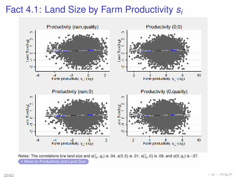
Fact 4.1: Land Size by Farm Productivity si

Notes: The correlations b/w land size and s(ζi ,qi ) is .04, s(0,0) is .01, s(ζi ,0) is .09, and s(0,qi ) is -.07.More on Productivity and Land Size

23/62

Fact 4.2: Capital by Farm Productivity

24/62

Fact 4.3: Capital-Land Ratio by Farm Productivity

25/62

Fact 4.4: Yield by Farm Productivity

Notes: The correlation is . 77 (N .70, C .71, S .81).

26/62

Fact 4.5 Capital Productivity by Farm Productivity


27/62

Fact 5. Evidence by Farm Size

I Fact 5.1: Capital increases with farm size

I Fact 5.2: Capital-land ratio is roughly constant across farmsize.

I Fact 5.3: Yield (output per unit of land) weakly declineswith farm size.

I Fact 5.4: Capital productivity (output per unit of capital) isroughly constant with farm size.

28/62

Fact 5.3: Yield by Farm Size

Notes: The correlation is -.18 (N -.28, C -.08, S -.33).

29/62

Fact 5.4: Capital Productivity by Farm Size

Notes: The correlation is .03 (N .08, C .00, S -.02).

30/62

Assessing Productivity Effect of Misallocation

31/62

Misallocation and ProductivityI Solve efficient allocation of capital and land across a fixed set of

heterogeneous farmers.

I Planner chooses allocations to maximize agricultural outputgiven fixed amounts of capital and land:

Y e = max{ki ,li}

∑i

si (kαki lαl

i )γ,

subject to:

K = ∑i

ki ,

L = ∑i

li .

I Efficient allocation equates marginal products of capital and landand has a simple form, let zi ≡ s1/(1−γ)

i ,

kei =

zi

∑ziK , lei =

zi

∑ziL.

32/62

Main Reallocation Result

I The output (productivity) loss is defined as

Y a

Y e =∑ya

i

∑yei

= .330

where yi = si(kαk

i lαli

)γ, and yei is evaluated at efficient

allocations.

I That is, if we were to efficiently reallocate land and capital,aggregate output would increase by a factor of 3.

33/62

Reallocation Results

Output (Productivity) Loss (Y a/Y e)

Aggregate Median Min Max

Nationwide .330 – – –

Region .376 .429 .232 .564

District .436 .443 .163 .692

Traditional Authority .546 .578 .130 .878

Language .375 .326 .194 .818

Notes: Table reports ratio of actual to efficient output. By region, median is Center, min is North, max is

South.

34/62

Actual vs. Efficient Distribution

Bottom(%) Quartiles Top(%)0-1 1-5 5-10 1st 2nd 3rd 4th 10-5 5-1 1

Prod. si : .00 .00 .04 .11 .29 .47 1.95 2.80 4.03 9.67

Land:Actual 1.78 1.79 1.77 1.82 1.90 1.82 2.06 2.14 2.07 2.11Eff. .00 .00 .00 .01 .06 .17 13.30 25.67 49.54 231.02

Capital:Actual 2,105 2,530 5,465 6,688 8,513 4,819 3,800 3,968 2,933 2,695Eff. 0 0 7 37 196 509 38,014 73,344 141,550 660,054

Yield:Actual .00 .00 .02 .07 .18 .26 .38 .97 1.35 3.28Eff. .00 .00 .02 .07 .18 .26 .38 .97 1.35 3.28

Notes: Farm households are ranked according to farm productivity.

More on Actual vs. Efficient Inequality

35/62

Reallocation within Enumeration AreasLand Quality Check

36/62

Reallocation within Skill GroupsHuman Capital Check

Schooling Groups:No Schooling Dropouts Primary > Primary

Output Loss (Y a/Y e) .382 .290 .336 .463

Terrain-roughness Specific Skills:High Altitude Low Mid-Altitude Mid-Altitude

Plains Plateaus Plateaus Mountains

Output Loss (Y a/Y e) .262 .451 .480 .393

Notes: By education groups, no Schooling 24.83%, primary school dropouts 44.92%, primary 23.12%, and

more 7.14%.

37/62

Conclusion

1. We estimate productivity for household-farms. Excellentoutput and input data that also allows to control for land quality &rain shocks. We find little quantitative role of land quality &rain in accounting for output differentials across farms.

2. An efficient reallocation of capital and land across theexisting set of farmers increases agricultural output andtotal factor productivity by a factor of 3-fold.

3. Similar increase in productivity arises in reallocating withinregions, districts, and much narrower enumeration areas.Also within a wide set of factors such as language, humancapital, among others.

4. Productivity effects can be larger when allowing for endogenousproductivity investment, GE effects in the number of farms(increase in average farm size), selection, among others.

38/62

Measurement Error

I There are very few missing observations.

I Our understanding from the World Bank field managers incharge of the data collection is that this is due to the fact thatrespondents took the survey as ’official’.

I Internal consistency reliability checks are conducted (e.g.,individuals are asked total sales, and also sales by crop; theinterviewer checks that the sums coincide).

I We exclude outliers: Trimming the top and bottom 1%

I While not in our benchmark, to deal with potential recall andtelescopic measurement error in agriculture production andactivities we re-conduct our exercise for households that wereinterviewed within the three months after and including March(the harvest month).

Back

39/62

Fact 4.1 Capital vs. Farm Size

Notes: The correlation is .42 (N .37, C .48, S .35).

40/62

Fact 4.2 Capital-Land Ratio vs. Farm Size

Notes: The correlation is -.20 (N -.31, C -.05, S .-30).

41/62

Hours vs. Farm Size

Notes: The correlation is .45 (N .45, C .47, S .41).

42/62

Capital-Labor Ratio vs. Farm Size

Notes: The correlation is .07 (N -.03, C .16, S .03).

43/62

Labor Productivity vs. Farm Size

Notes: The correlation is .13 (N .03, C .21, S -.01).

44/62


I Global Agro-Ecological Zone (GAEZ):

Use latitude and longitude coordinates. Within Malawi we canidentify four zones.

RegionsFull Sample North Center South

Tropic-warm/semiarid 47.49 4.31 63.13 51.90Tropic-warm/subhumid 35.23 50.47 11.12 47.41Tropic-cool/semiarid 10.55 10.24 24.17 .68Tropic-cool/subhumid 6.72 34.98 1.58 .11

100.00 100.00 100.00 100.00

In rural areas, population distribution across regions is 17.49% in NorthernMalawi, 34.89% in Center, and 47.62% in Southern Malawi.

Back

45/62

Land Quality Dimensions (continued)Regions

Full Sample North Center South

Slope:Flat 56.24 (2.5) 57.07 (3.6) 54.84 (2.4) 56.98 (2.4)Slight 32.54 (4.9) 27.99 (5.8) 34.77 (3.7) 32.45 (5.7)Moderate 8.14 (6.2) 8.68 (8.0) 8.24 (5.4) 7.88 (6.5)Steep/Hilly 3.08 (10.3) 6.26 (14.6) 2.15 (6.7) 2.68 (10.7)

100.00 (3.5) 100.00 (4.9) 100.00 (2.9) 100.00 (3.5)

Erosion, qeroi :

No Erosion 60.69 51.62 61.82 62.96Low 26.66 31.56 25.82 25.60Moderate 7.57 10.23 7.65 6.60High 5.08 6.59 4.71 4.84

100.00 100.00 100.00 100.00

Soil Quality, qsqi :

Good 45.95 48.86 44. 91 45.72Fair 42.63 43.47 40.51 43.89Poor 11.42 7.67 14.58 10.39

100.00 100.00 100.00 100.00Notes: Regressing ln(slope) on self-reported slope dummies we find all dummies significant, and capturing 17% ofthe slope variation.

46/62


Full Samp. North Center South

Nutritient Availability, qnai :

No or Slight Rest. 59.63 28.29 47.05 80.37Moderate Rest. 22.13 43.13 25.74 11.76Severe Rest. 13.51 22.24 18.24 6.84Very Severe Rest. .42 6.34 1.20 1.03

100.00 100.00 100.00 100.00

Nutritient Retention Capacity, qnci :

No or Slight Rest. 65.12 43.42 51.81 82.85Moderate Rest. 28.81 44.24 38.38 16.12Severe Rest. 1.51 6.00 1.31 .00Very Severe Rest. .51 6.34 1.46 .00

100.00 100.00 100.00 100.00

Rooting Conditions, qrci :

No or Slight Rest. 63.75 38.53 72.36 66.70Moderate Rest. 15.69 26.19 10.80 15.42Severe Rest. 14.01 26.78 9.05 12.96Very Severe Rest. 2.33 2.15 .76 3.55

100.00 100.00 100.00 100.00

47/62


Full Samp. North Center South

Oxygen Availability to Roots, qoari :

No or Slight Rest. 85.50 84.40 81.67 88.71Moderate Rest. 6.35 6.11 4.12 8.08Severe Rest. 3.42 3.14 5.25 2.18Very Severe Rest. .67 .00 1.93 .00

100.00 100.00 100.00 100.00

Excess Salts, qexsi :

No or Slight Rest. 91.35 84.40 90.81 94.31Moderate Rest. 3.50 5.94 .70 4.66Severe Rest. .84 3.32 .73 .00Very Severe Rest. .25 .00 .73 .00

100.00 100.00 100.00 100.00

Toxicity, qtoxi :

No or Slight Rest. 93.08 84.40 90.81 97.93Moderate Rest. 1.99 7.10 .70 1.05Severe Rest. .63 2.15 .73 .00Very Severe Rest. .25 .00 .73 .00

100.00 100.00 100.00 100.00

48/62


RegionsFull Samp. North Center South

Workability, qwi :

No or Slight Rest. 48.31 37.25 69.47 36.87Moderate Rest. 27.83 27.88 13.46 38.34Severe Rest. 15.67 26.37 9.28 16.42Very Severe Rest. 3.97 2.15 .76 6 .99

100.00 100.00 100.00 100.00

Back

49/62

Dispersion (Variance) of Land Quality

By Geographic Aggregation Level:Full Samp. Regions Districts Enum. Area

Land Size, Li : .618 .595 .545 .488

Quality-Adjusted Land Size:q0

i Li .647 .625 .568 .485q1

i Li .636 .618 .566 .486q2

i Li .704 .691 .609 .510q3

i Li .942 .927 .736 .514


Back

50/62

Rain Shocks, ζi

I Annual Precipitation (total rainfall, mm) (last 12 months), andaverage 12-month total rainfall (mm) in last 10 years (since2001).

To compute the unanticipated amount of rain in 2010/11, u2010,we remove from the current annual precipiation the average oftotal rainfall of the past 10 years,

ln total rainfall2010 = cons+β lnaverage total rainfallsince2001 +u2010(1)

I Precipitation of wettest quarter (mm) (within last 12 months),and average precipitation of wettest quarter (mm) in last 10years (since 2001).1

Back

1For now, we ignore temperature and greenness.

51/62

Productivity si vs. Land Quality Index qi : By Region

Notes: The correlations b/w land quality and si is -.14 in the full sample, -.13 in the Northern region, -.01 in the

Center region, and -.21 in the Southern region.52/62

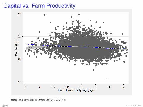
Capital vs. Farm Productivity


53/62

Capital-Land Ratio vs. Farm Productivity


54/62

Hours vs. Farm Productivity


55/62

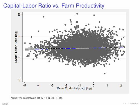
Capital-Labor Ratio vs. Farm Productivity

Notes: The correlation is .04 (N .11, C -.00, S .04).

56/62

Labor Productivity vs. Farm Productivity


57/62

Variance Decomposition yiζi qi ζi qi ζi qi ζi qiY Y % N N % Y N % N Y %

var(y) 1.423 100.0 1.423 100.0 1.423 100.0 1.423 100.0

var(s) .968 68.0 .937 65.8 .943 66.3 .962 67.6

var(ζ) .007 .5 – – .007 .5 – –

var(f (k ,ql)) .297 20.9 .303 21.3 .303 21.3 .297 20.9

2cov(s,ζ) -.012 -.8 – – -.012 -.8 – –

2cov(s, f (k ,ql)) .156 11.0 .172 12.1 .170 11.9 .158 11.12cov(s,θk k) .082 5.8 .084 5.9 .082 5.8 .086 6.02cov(s,θl q) -.012 -.8 – – – – -.014 -1.02cov(s,θl l) .086 6.0 .088 6.2 .088 6.2 .086 6.0

2cov(ζ, f (k ,ql)) .003 – – .3 .004 .3 – –2cov(ζ,θk k) .003 .2 – – .003 .3 – –2cov(ζ,θl q) -.000 -.0 – – – – – –2cov(ζ,θl l) .000 .0 – – .000 .0 – –


58/62

Variance Decomposition yi , by region (with qi and ζi )

RegionsFull S. % North % Center % South %

var(y) 1.423 100.0 1.252 100.0 1.156 100.0 1.432 100.0

var(s) .968 68.0 .735 58.7 .726 62.8 1.054 73.6

var(ζ) .007 .5 .004 .3 .012 1.0 .004 .3

var(f (k ,ql)) .297 20.9 .292 23.3 .324 28.0 .263 18.4

2cov(s,ζ) -.012 -.8 -.006 -.5 -.024 -2.1 .001 .1

2cov(s, f (k ,ql)) .156 11.0 .204 16.3 .116 10.0 .103 7.2

2cov(ζ, f (k ,ql)) .003 .2 -.001 -.1 .004 .3 .000 .0

Notes: All variables have been logged.Back

59/62

Productivity si vs. Land Size

Notes: The correlations b/w land size and s(ζi ,qi ) is .05, s(0,0) is .01, s(ζi ,0) is .09, and s(0,qi ) is -.06. Back

60/62

Inequality

Data EfficientProductivity Land Capital Output {li ,ki ,yi}

Variance .909 .841 1.715 1.161 4.29775-25 3.61 2.78 4.95 4.22 12.2090-10 10.82 7.67 24.21 19.96 177.12Gini .51 .50 .72 .63 .94

Notes: To compute the variance, variables are in logs. Ouptut is net of quality and rain shocks.

61/62

Inequality By Region

Northern Region : Data EfficientProductivity Land Capital Output {li ,ki ,yi}

Variance .688 .821 1.619 1.191 3.25375-25 2.83 3.21 5.08 4.14 9.6590-10 7.82 9.27 24.11 15.46 87.46

Center Region : Data EfficientProductivity Land Capital Output {li ,ki ,yi}

Variance .700 .672 1.886 1.136 3.31075-25 2.67 2.79 5.26 3.57 8.4890-10 7.14 7.32 29.68 12.86 71.83

Southern Region : Data EfficientProductivity Land Capital Output {li ,ki ,yi}

Variance 1.024 .687 1.469 1.398 4.84375-25 3.36 2.70 4.51 4.39 13.9590-10 17.91 7.44 19.45 28.18 529.90

Back

62/62

land misallocation and productivity - imf · land misallocation and productivity diego restuccia...

Documents