file: cebrat1.tex, April 1, 2004

Kohonen’s self-organizing maps as applied to graphical

visualization of some yeast DNA data – Supplement: PLOTS

Anna Bartkowiak1, Adam Szustalewicz1

StanisÃlaw Cebrat2, PaweÃl Mackiewicz2

1 Institute of Computer Science, University of WrocÃlaw2Institute of Genetics and Microbiology, University of WrocÃlaw

Abstract

We analyze a set of data describing N=3300 yeast genes, each gene characterizedby d=13 variables (traits). First we performed an explorative data analysis andstated a high multivariate kurtosis. Next we clustered the data and visualized themusing Kohonen’s self-organizing maps. This has permitted us to get an idea how thedata are distributed in the multivariate space.

Keywords: explorative data analysis, clustering, self-organizing maps, yeast genome.

2 The data

We consider spider plots representing yeast genes.An exemplary spider-plot is shown in Figure 1.

Figure 1 Spider plot for the yeast gene YBL008w (HIR1); position 1 - the walker visitsevery first nucleotide of codons and moves a unit up if the nucleotide is G, down if it is C,right if it is A and left if it is T; position 2 - the walker visits every second nucleotide ofcodons, and proceeds the same way; position 3 - the walker visits every third nucleotide ofcodons, and proceeds the same way . {paa.jpg}

1

3 Exploratory analysis of the data set

Every spider-plot was characterized by 13 variables: x1, y1, x2, y2, x3, y3, angle1, angle2,angle3, length of the ORF, and rho1, rho2, rho3.

Pairwise scatter-plots of the variables angle1, angle2, angle3, rho1, rho2, rho3 andlength, crossed with the variables x1, y1, x2, y2, x3, y3, are shown in Figure 2.

Figure 2: Scatter-plot matrix displaying pair-wise dependencies among variables’y’=angle1, angle2, angle3, rho1, rho2, rho3, length, put against the variables ’x’ = x1,y1, x2, y2, x3, y3. {scatmgm.jpg }

2

4 Visualization of the data using Kohonen’s self-organizing

maps

Training the prototypes. During the process of training the prototypes, initialized froma PC plane, approach the data points and adapt themselves to the (d-dimensional) densitydistribution of the data. This is done iteratively.

−2

0

2

−20

2−1

0

1

2

3

rho1

DATA: random sample n=225

rho2

rho3

−2

0

2

−20

2−1

0

1

2

3

rho1

After training, general view

rho2

rho3

−1012−1012−1

−0.5

0

0.5

1

1.5

2

rho1

After training, 1st detailed view

rho2

rho3

−1 0 1 2−1012−1

−0.5

0

0.5

1

1.5

2

rho1

After training, 2nd detailed view

rho2

rho3

Figure 3. Training the SOM for 3–dimensional data. sampled from the ’genes’ data.Shown using two different color palettes. Subplot 1 (upper row) shows a 3D plot of then=225 points included in the sample. Subplot 2 (upper row) shows the prototypes aftertraining – in the same layout, as the data. The prototypes are linked together by segmentsof various length and designate a complicated surface. Subplots 3 and 4 (bottom row) showenlarged fragments of subplot 2, facing the sides rho2 and rho1 {cube2.eps, cube4.eps}

In Figure 3 we show an example of constructing the map (SOM) for 3-dimensional data.We took for that purpose a sample of the GENES data containing n=225 data vectors (theGENES data of size 3300 × 13 were first standardized to have column means equal toone and unit variances). We took for this example only 3 variables: rho1, rho2 and rho3.The proposed (default) configuration of the map was: 12 × 6 (see Matlab SOM Toolbox,Vesanto et al., 2000). The starting values of the prototypes were designated by default asregular points located on the PC plane.

3

−20

2

−2

0

2

−1

0

1

2

3

rho1

DATA: random sample n=225

rho2

rho3

−2

0

2

−20

2−1

0

1

2

3

rho1

After training, general view

rho2

rho3

−10

12

−1012−1

0

1

2

rho1rho2

Enlarged view, facing rho2

rho3

−1 0 1 2−10

12

−1

0

1

2Enlarged view, facing rho1

rho1rho2

rho3

Figure 3a. Training the SOM for 3–dimensional data. The same, as in previous Figure,however a different color palette was used. { cube4.eps}

Initially, the prototypes were positioned on a plane and linked together by a regulargrid. During the process of training, the prototypes have adapted themselves to the data.With movements of the prototypes, the initial plane has swelled, bulged and recurvedto a complicated surface. However, the initial connections ordering the prototypes haveremained. The final positions of the prototypes, together with their links, are shown in thesecond exhibit. More detailed views of the enlarged surface – when looking from the rho2and rho1 axis – are shown in subplot 3 and subplot 4 of the figure.

Figure 3a shows the same, as Figure 3, however using a different color palette.

4

Figure 4. Maps constructed for the entire GENES data. Color shades (identified bythe color-bar at right) indicate for distances between neighboring prototypes. Dark huesmean big distances. The dark dots indicate the reference vectors positioned in the map.{umatij.jpg, map2j.jpg}

5

Map size 13x11Hits

Figure 5. Displays of the number of hits into map units. Upper plot: Hits indicated byshadowed sizes of the hexagons. Bottom plots: Digital displays of the counts. The numberof hits is differentiated from min=3 to max=76. {map3.eps, map4aj.jpg}

6

4.1 Which data vectors are represented in corners of the map

Not shown.

4.2 Interpretation of directions of the map

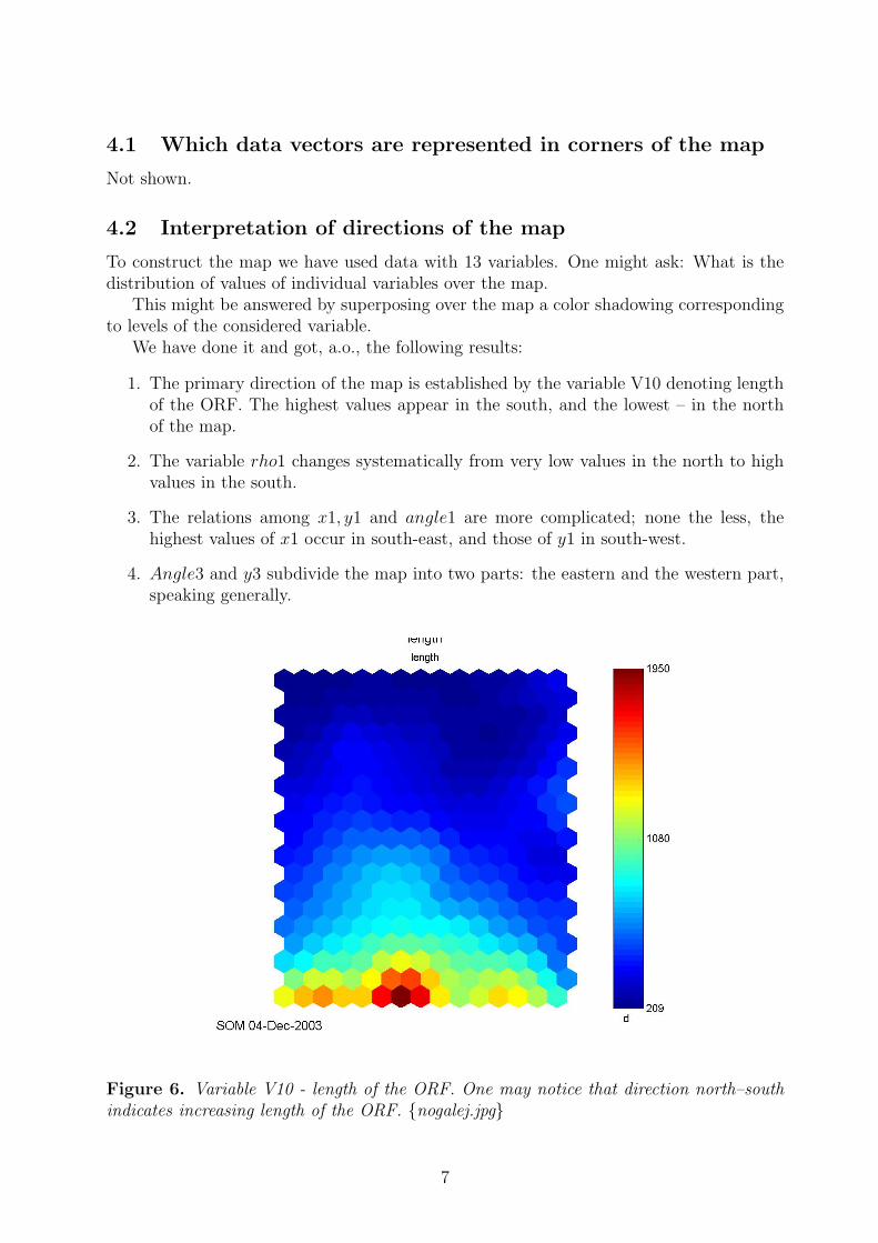
To construct the map we have used data with 13 variables. One might ask: What is thedistribution of values of individual variables over the map.

This might be answered by superposing over the map a color shadowing correspondingto levels of the considered variable.

We have done it and got, a.o., the following results:

1. The primary direction of the map is established by the variable V10 denoting lengthof the ORF. The highest values appear in the south, and the lowest – in the northof the map.

2. The variable rho1 changes systematically from very low values in the north to highvalues in the south.

3. The relations among x1, y1 and angle1 are more complicated; none the less, thehighest values of x1 occur in south-east, and those of y1 in south-west.

4. Angle3 and y3 subdivide the map into two parts: the eastern and the western part,speaking generally.

Figure 6. Variable V10 - length of the ORF. One may notice that direction north–southindicates increasing length of the ORF. {nogalej.jpg}

7

Figure 7. Component planes characterizing the 1st leg of the spider. Again, the directionnorth–south is generally connected with increasing length of the 1st leg. {noga1j.jpg}

8

Figure 8. Component planes characterizing the 2nd and the 3rd leg of the ORFs.{noga2j.jpg, noga3j.jpg}

9

d −2.04

−0.417

1.21angle1

d −1.22

0.549

2.32x1

d −1.58

0.25

2.08y1

d −1.19

0.417

2.03ro1

d −1.07

0.0986

1.27angle3

d −1.97

−0.4

1.17x3

d −1.9

−0.483

0.937

y3

d 0

0.886

2.54ro3

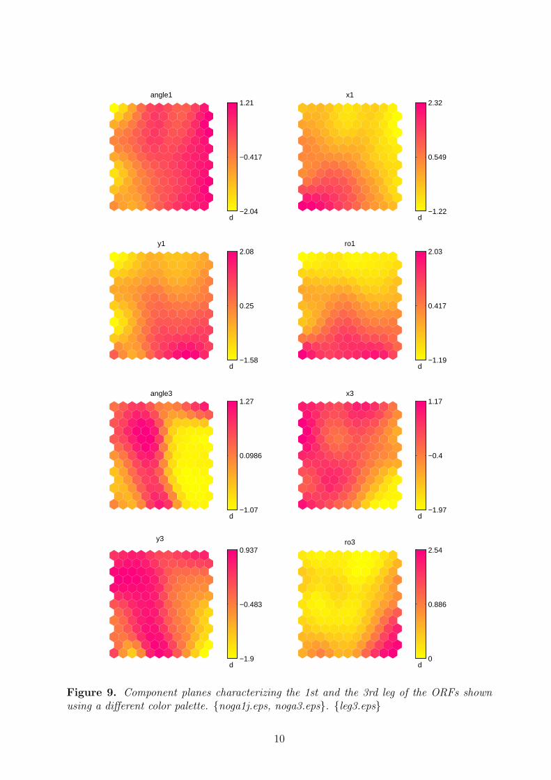
Figure 9. Component planes characterizing the 1st and the 3rd leg of the ORFs shownusing a different color palette. {noga1j.eps, noga3.eps}. {leg3.eps}

10

5 Discussion and concluding remarks

We have presented the method of Kohonen’s self-organizing maps (SOMs) and shown itsperformance on a true data set describing 6330 Open Reading Frames (ORFs) of the yeastgenome.

We have shown that the SOM method permits for a meaningful graphical visualizationof multivariate data cloud in a planar ’map’. In our case data points from R13 could berepresented in a 2-dimensional plane.

We have shown also that the SOM method enables finding objects which have similarmorphology. In the analyzed data we were able finding in an easy way groups of genes,which have similar prevalence of purines and pyramidines in the first and second nucleotideof their codons.

There are many clustering methods, however the SOM method belongs to the few oneswhich permit for a simultaneous visualization of the clusters with preserving their topologyin the multivariate data space.

References

[1] Avery P.J., Henderson D.A. (1999) Fitting Markov chain models to discrete state series suchas DNA sequences. Appl. Statistics, 48, Part 1, 53–61.

[2] Bartkowiak A., Szustalewicz A., Evelpidou N., Vassilopoulos A. (2003) Choosing data vectorsrepresenting a huge data set: a comparison of Kohonen’s maps and the neural gas method.Proc. F irst Int. Conf. on Environmental Research and Assessment, Bucharest, Romania, pp.561–572, print on CD–ROM, c©Ars Docendi P. H, Bucharest, Romania.

[3] Braun J.V., Muller H-G. (1998) Statistical methods for DNA sequence segmentation. Sta-tistical Science, 13, No. 2, 142–162.

[4] Cebrat S., Mackiewicz P., Dudek M.R. (1998) The role of the genetic code in generating newcoding sequences inside existing genes. Biosystems, 45 (2), 165–176.

[5] Cebrat S., Dudek M.R. (1998) The effect of DNA phase structure on DNA walks. TheEuropean Physical Journal B., 3 271–276.

[6] Cebrat S., Dudek M., Rogowska A. (1997) Asymmetry in nucleotide composition of sense andantisense strands as a parameter for discriminating open reading frames as protein codingsequences. J. Appl. Genet. 38, No. 1, 1–9.

[7] Dougherty E.R., Barrera J., et al. (2002) Inference from clustering with application to gene-expression microarrays. Journal of Computational Biology 9, Nb. 1, 105–126.

[8] Kamb A., Wang Ch., et al. (1995) Software Trapping: A strategy for finding genes in largegenomic regions. Computers and Biomed. Research 28, 140–153.

[9] Kiviluoto K. (1996) Topology preservation in self-organizing maps. Proceedings ICNN’96,V. 1, June 1996, IEEE Neural Networks Council, Piscataway, New Jersey, USA, 294–299.

[10] Kohonen T. (1995) Self-Organizing Maps. Springer Series in Information Sciences, V. 30,Berlin.

11

[11] Mackiewicz P., Kowalczuk M., Mackiewicz D., Nowicka A., Dudkiewicz M., Laszkiewicz A.,Dudek M.R., Cebrat S. (2002) How many protein–coding genes are there in the Saccha-romyces cerevisiae genome? Yeast 19(7), 619–629.

[12] Mackiewicz P., Kowalczuk M., Fita M., Cebrat S., Dudek M.R. (1997) Asymmetry of codingversus noncoding strand in coding sequences of different genomes. Microbial & ComparativeGenomics, 2, No. 4, 259–268.

[13] Mardia K. V. (1980) Tests of univariate and multivariate normality. In: P. R. Krishnaiah(Ed.), Handbook of Statistics. Vol. 1. North-Holland Publishing Company. 279–320.

[14] Mardia, K. V., Kent, J. T., Bibby, J. M. (1979) Multivariate Analysis. Academic Press,London.

[15] Muri, F. (1998) Modelling bacterial genomes using hidden Markov models. COMPSTAT1998, Invited and Contributed Papers, 89–100.

[16] Prum B., Rodolphe F., de Turckheim E. (1995) Finding words with unexpected frequenciesin desoxyribonucleic acid sequences. J.R. Statist. Soc. B, 57, No. 1., 205–220.

[17] Rousseeuw P.J., van Driessen K. (1999) A fast algorithm for the minimum covariance deter-minant. Technometrics 41, pp. 212–223.

[18] Venna J., Kaski S. (2001) Neighborhood preservation in nonlinear projection methods: Anexperimental study. In: G. Dorffner, H. Bischof, and K. Hornik (Eds), Proceedings ICANN2001, Vienna. Springer, Berlin, pp. 485–491.

[19] Vesanto J. (1999) SOM–based data visualizing methods. Intelligent Data Analysis, 3(2), pp.111–126.

[20] Vesanto J., Himberg J., Alhoniemi E., Parhankangas J. (2000) SOM Toolbox for Matlab5. SOM Toolbox Team, Helsinki University of Technology, Finland, Libella Oy, Espoo, pp.1–54. http://www.cis.hut.fi/projects/somtoolbox, Version 0beta 2.0, Nov. 2001.

[21] smorf http://smorfland.microb.uni.wroc.pl/

12