klamath river tmdl model - home page | california state ... · klamath river model for tmdl...
TRANSCRIPT
APPENDIX 6
Model Configuration and Results
Klamath River Model for TMDL Development
Fourth Revision: December 2009 Third Revision: June 2009
Second Revision: September 2008 First Revision: September 2007
Original: September 2005
Prepared for: U.S. Environmental Protection Agency Region 9
U.S. Environmental Protection Agency Region 10 North Coast Regional Water Quality Control Board
Oregon Department of Environmental Quality
Prepared by: Tetra Tech, Inc.
Model Configuration and Results
Contents
1.0 INTRODUCTION ...........................................................................................1
2.0 MODELING APPROACH ..............................................................................3 2.1 MODEL SELECTION ................................................................................................... 3 2.2 MODEL ENHANCEMENTS........................................................................................... 7
2.2.1 BOD/OM Unification ........................................................................................ 7 2.2.2 Two-state Algae Transformation Algorithm in Lake Ewauna .......................... 8 2.2.3 Monod-Type SOD and OM Decay .................................................................. 11 2.2.4 pH Simulation Module in RMA ...................................................................... 12 2.2.5 OM-dependent Light Extinction Formulation in RMA................................... 12 2.2.6 Reaeration Formulation Modification.............................................................. 12 2.2.7 Dynamic OM Partitioning................................................................................ 13 2.2.8 Periphyton Carrying Capacity.......................................................................... 13 2.2.9 Additional Shading in RMA ............................................................................ 14 2.2.10 Second Order Polynomial Spillway Representation...................................... 14
2.3 MODEL CONFIGURATION......................................................................................... 15 2.3.1 Segmentation/Computational Grid Setup ........................................................ 15
2.3.1.1 Segmentation of River and Reservoir Segments ...................................... 17 2.3.1.2 Segmentation of the Klamath Estuary Segment ...................................... 17
2.3.2 State Variables ................................................................................................ 18 2.3.3 Boundary Conditions ....................................................................................... 20
2.3.3.1 Model Segment 1: Link River................................................................... 21 2.3.3.2 Model Segment 2: Lake Ewauna to Keno Dam....................................... 23 2.3.3.3 Model Segment 3: Keno Dam to J.C. Boyle Reservoir (Keno Reach)..... 26 2.3.3.4 Model Segment 4: J.C. Boyle Reservoir.................................................. 26 2.3.3.5 Model Segment 5: Bypass/Full Flow Reach............................................ 27 2.3.3.6 Model Segment 6: Copco Reservoir ......................................................... 27 2.3.3.7 Model Segment 7: Iron Gate Reservoir .................................................... 28 2.3.3.8 Model Segment 8: Iron Gate Dam to Turwar ........................................... 29 2.3.3.9 Model Segment 9: Klamath Estuary (Turwar to the Pacific Ocean) ........ 34
2.3.4 Initial Conditions ............................................................................................. 36 2.4 MODELING ASSUMPTIONS, LIMITATIONS, AND SOURCES OF UNCERTAINTY ........... 36
2.4.1 Assumptions..................................................................................................... 36 2.4.2 Limitations ...................................................................................................... 37 2.4.3 Sources of Uncertainty..................................................................................... 38
3.0 MODEL TESTING .......................................................................................40 3.1 MONITORING LOCATIONS........................................................................................ 41 3.2 HYDRODYNAMIC CALIBRATION .............................................................................. 45 3.3 WATER QUALITY CALIBRATION.............................................................................. 45
3.3.1 Link River (Model Segment 1) ....................................................................... 49 3.3.2 Lake Ewauna-Keno Dam (Model Segment 2)................................................ 50 3.3.3 Keno Dam to J.C. Boyle Reservoir (Model Segment 3)................................. 52 3.3.4 J.C. Boyle Reservoir (Model Segment 4) ....................................................... 52 3.3.5 Bypass/Full Flow Reach (Model Segment 5) ................................................. 53
ii
Model Configuration and Results
3.3.6 Copco Reservoir (Model Segment 6) ............................................................. 54 3.3.7 Iron Gate Reservoir (Model Segment 7)......................................................... 54 3.3.8 Iron Gate Dam to Turwar (Model Segment 8)................................................ 54 3.3.9 Klamath Estuary - Turwar to the Pacific Ocean (Model Segment 9) ............. 56
REFERENCES ...................................................................................................58
APPENDIX A pH Simulation Module Equations – From Chapra, 1997 APPENDIX B System Geometry - Excerpt from the PacifiCorp, 2005 Report APPENDIX C Klamath Estuary EFDC Grid APPENDIX D Determination of Accretions for Tributaries from Iron Gate Dam to
Turwar - Excerpt from the PacifiCorp, 2004 Report APPENDIX E Calibration Results for Lake Ewauna to Keno Dam (Modeling Segment
2) APPENDIX F Calibration Results for Keno Dam to J. C. Boyle Reservoir (Modeling
Segment 3) APPENDIX G Calibration Results for J.C. Boyle Reservoir (Modeling Segment 4) APPENDIX H Calibration Results for Bypass/Full Flow Reach (Modeling Segment 5) APPENDIX I Calibration Results for Copco Reservoir (Modeling Segment 6) APPENDIX J Calibration Results for Iron Gate Reservoir (Modeling Segment 7) APPENDIX K Calibration Results for Iron Gate Dam to Turwar (Modeling Segment 8) APPENDIX L Calibration Results for Turwar to the Pacific Ocean (Modeling Segment
9)
iii
Model Configuration and Results
iv
Acknowledgments Completion of the Klamath River Hydrodynamic and Water Quality Model for TMDL development was made possible by the generous support and responsiveness of many people. The authors would like to acknowledge the following professionals, in particular, for their contributions:
Ben Cope U.S. Environmental Protection Agency, Region 10 Clayton Creager North Coast Regional Water Quality Control Board Michael Deas Watercourse Engineering, Inc. Mark Filippini U.S. Environmental Protection Agency, Region 10 Susan Keydel U.S. Environmental Protection Agency, Region 9 Steve Kirk Oregon Department of Environmental Quality David Leland North Coast Regional Water Quality Control Board Gail Louis U.S. Environmental Protection Agency, Region 9 Bryan McFadin North Coast Regional Water Quality Control Board Matt St. John North Coast Regional Water Quality Control Board Daniel Turner Oregon Department of Environmental Quality
Andrew Parker, Rui Zou, and Mustafa Faizullabhoy led Tetra Tech’s model development and application effort.
Model Configuration and Results
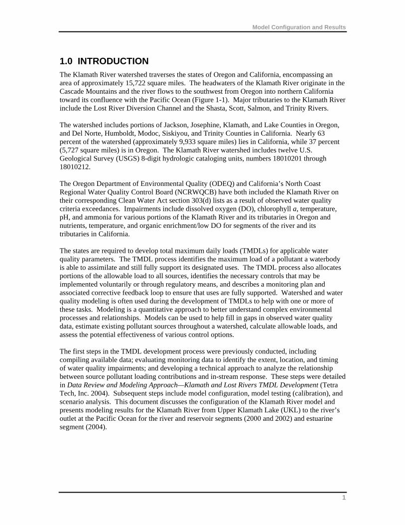
1.0 INTRODUCTION The Klamath River watershed traverses the states of Oregon and California, encompassing an area of approximately 15,722 square miles. The headwaters of the Klamath River originate in the Cascade Mountains and the river flows to the southwest from Oregon into northern California toward its confluence with the Pacific Ocean (Figure 1-1). Major tributaries to the Klamath River include the Lost River Diversion Channel and the Shasta, Scott, Salmon, and Trinity Rivers. The watershed includes portions of Jackson, Josephine, Klamath, and Lake Counties in Oregon, and Del Norte, Humboldt, Modoc, Siskiyou, and Trinity Counties in California. Nearly 63 percent of the watershed (approximately 9,933 square miles) lies in California, while 37 percent (5,727 square miles) is in Oregon. The Klamath River watershed includes twelve U.S. Geological Survey (USGS) 8-digit hydrologic cataloging units, numbers 18010201 through 18010212. The Oregon Department of Environmental Quality (ODEQ) and California’s North Coast Regional Water Quality Control Board (NCRWQCB) have both included the Klamath River on their corresponding Clean Water Act section 303(d) lists as a result of observed water quality criteria exceedances. Impairments include dissolved oxygen (DO), chlorophyll a, temperature, pH, and ammonia for various portions of the Klamath River and its tributaries in Oregon and nutrients, temperature, and organic enrichment/low DO for segments of the river and its tributaries in California. The states are required to develop total maximum daily loads (TMDLs) for applicable water quality parameters. The TMDL process identifies the maximum load of a pollutant a waterbody is able to assimilate and still fully support its designated uses. The TMDL process also allocates portions of the allowable load to all sources, identifies the necessary controls that may be implemented voluntarily or through regulatory means, and describes a monitoring plan and associated corrective feedback loop to ensure that uses are fully supported. Watershed and water quality modeling is often used during the development of TMDLs to help with one or more of these tasks. Modeling is a quantitative approach to better understand complex environmental processes and relationships. Models can be used to help fill in gaps in observed water quality data, estimate existing pollutant sources throughout a watershed, calculate allowable loads, and assess the potential effectiveness of various control options. The first steps in the TMDL development process were previously conducted, including compiling available data; evaluating monitoring data to identify the extent, location, and timing of water quality impairments; and developing a technical approach to analyze the relationship between source pollutant loading contributions and in-stream response. These steps were detailed in Data Review and Modeling Approach—Klamath and Lost Rivers TMDL Development (Tetra Tech, Inc. 2004). Subsequent steps include model configuration, model testing (calibration), and scenario analysis. This document discusses the configuration of the Klamath River model and presents modeling results for the Klamath River from Upper Klamath Lake (UKL) to the river’s outlet at the Pacific Ocean for the river and reservoir segments (2000 and 2002) and estuarine segment (2004).
1
Model Configuration and Results
Figure 1-1. Extent of the Klamath River watershed
2
Model Configuration and Results
2.0 MODELING APPROACH
2.1 Model Selection
To support TMDL development for the Klamath River system, the need for an integrated receiving water hydrodynamic and water quality modeling system was identified. The following model capabilities were identified as being necessary to support TMDL development. The model must be
Capable of predicting hydrodynamics, nutrient cycles, DO, temperature, pH, and other parameters and processes pertinent to the TMDL development effort;
Capable of simulating the multiple flow control structures along the length of the Klamath River;
Dynamic (time-variable) and thus capable of representing the highly variable flow and water quality conditions within years and between years;
Capable of considering the steep channel slope of the Klamath River; and
Capable of representing conditions in the Klamath Estuary. A model for the Klamath River had already been developed by PacifiCorp to support studies for the Federal Energy Regulatory Commission Hydropower relicensing process (Watercourse Engineering, Inc. 2004) when this project began. The version of the model available in 2004 is hereafter referred to as the PacifiCorp Model. The PacifiCorp Model and other models, including the operational models MODSIM and CALSIM, were evaluated for applicability to Klamath River TMDL development (Tetra Tech, Inc. 2004). NCRWQCB, ODEQ, and the U.S. Environmental Protection Agency (EPA) determined that the existing PacifiCorp Model would provide the optimal basis, after making some enhancements, for TMDL model development. Section 2.2 provides a description of the enhancements made to the PacifiCorp Model. It should be noted that PacifiCorp has since updated the model after receiving comments from reviewers (PacifiCorp 2005). The original PacifiCorp Model consisted of Resource Management Associates (RMA) RMA-2 and RMA-11 models and the CE-QUAL-W2 model. Specifically, the RMA-2 and RMA-11 models were applied for Link River (which is the stretch of the Klamath River from UKL to Keno Dam), Keno Dam to J.C. Boyle Reservoir, Bypass/Peaking Reach (hereafter referred to as the Bypass/Full Flow Reach), and Iron Gate Dam to Turwar. RMA-2 simulates hydrodynamics, while RMA-11 represents water quality processes. The CE-QUAL-W2 model was applied for Lake Ewauna-Keno Dam, J.C. Boyle Reservoir, Copco Reservoir, and Iron Gate Reservoir. In addition to addressing the model needs identified above, the PacifiCorp Model
Uses hydrodynamic and water quality models with a proven track record in the environmental arena, including historical application to the Klamath River;
Has already been reviewed by most stakeholders in the watershed;
Can be directly compared to ODEQ, NCRWQCB and tribal water quality criteria;
Has been preliminarily calibrated for the Klamath River and its applicability demonstrated; and
Uses the public domain model CE-QUAL-W2 and a version of RMA that can be distributed to the public for purposes of TMDL application.
3

Model Configuration and Results
Because the estuarine portion of the Klamath River (Turwar to the Pacific Ocean) was not included in the original PacifiCorp Model, it was necessary to identify a model appropriate for modeling that portion of the river. After reviewing a 2004 bathymetric survey and grab, multiprobe, and cross-sectional profile data, it was determined that a laterally averaged 2-D model, such as CE-QUAL-W2, was not the ideal choice for modeling the estuarine portion of the Klamath River. Hydrodynamics and water quality within the estuary are highly variable spatially and throughout the year and are greatly influenced by time of year, river flow, tidal cycle, and location of the estuary mouth (which changes because of sand bar movement). Additionally, transect temperature and salinity data in the lower estuary showed significant lateral variability, as did DO to a lesser extent. The Environmental Fluid Dynamics Code (EFDC), which is a full 3-D hydrodynamic and water quality model, was selected to model the complex estuarine environment instead. EFDC is an EPA-endorsed and widely applied 3-D model (particularly for TMDL development). EFDC allows for representing the complex geometry of the Klamath Estuary with a boundary-fitted, curvilinear grid. The model is capable of simulating important physical processes and features, such as the circulation pattern near the funnel-shaped mouth and islands. The mouth of the estuary is very wide; however, it does not open to the Pacific Ocean completely because of the presence of a sand bar. As a result, the estuary can communicate with the ocean only through a very narrow opening in the sand bar. Configuring a CE-QUAL-W2 grid for this portion of the system would likely result in a very wide segment at the downstream end of the river. The wide segment would be linked to a very narrow segment representing the opening in the sand bar. This configuration runs the risk of resulting in computational error because of the sudden change in segment width at the most dynamic portion of the system (Cole and Wells, 2003). Although it is impossible to simulate the evolution of the existing sand bar at the estuary mouth with available technology, EFDC can potentially be used to efficiently evaluate the implications of mouth locations on hydrodynamics and water quality. Hydrodynamics and water quality in the estuary are also highly variable throughout the year and are greatly influenced by time of year, river flow, tidal cycle, and location of the mouth. Hydrodynamic data also show significant lateral variability, as does DO to a lesser extent. It is desirable to apply a model that has the potential to represent this variability and EFDC is capable. Additional factors leading to the choice of EFDC for modeling the estuary include the following:
EFDC is capable of predicting hydrodynamics, nutrient cycles, DO, temperature, and other parameters and processes pertinent to the TMDL development effort for the estuarine section.
The EFDC model is dynamic (time-variable) and thus capable of representing the highly variable flow and water quality conditions within years and between years.
EFDC has a proven track record in the environmental arena—particularly with regard to TMDLs.
Model results can be directly compared to ODEQ, NCRWQCB and tribal water quality criteria.
EFDC is EPA-endorsed and supported and is included in the EPA TMDL Modeling Toolbox. It is a public domain model, fully transparent (i.e., model code), and is available free of charge. EPA also provides training and support on the application free of charge.
4
Model Configuration and Results
EFDC has a function for blocking flows between computational cells, and this allows for efficiently evaluating the effect of the location and size of the sand bar opening, with a single grid configuration.
The EFDC water quality module possesses a fully numerical sediment diagenesis module to predict sediment oxygen demand (SOD) and benthic nutrient flux based on organic loading to the waterbody. This improves the reliability of the model for DO and nutrient TMDLs. Although this component was not used in this study because of time and data limitations, it can be implemented in the future using the existing framework when sufficient data become available.
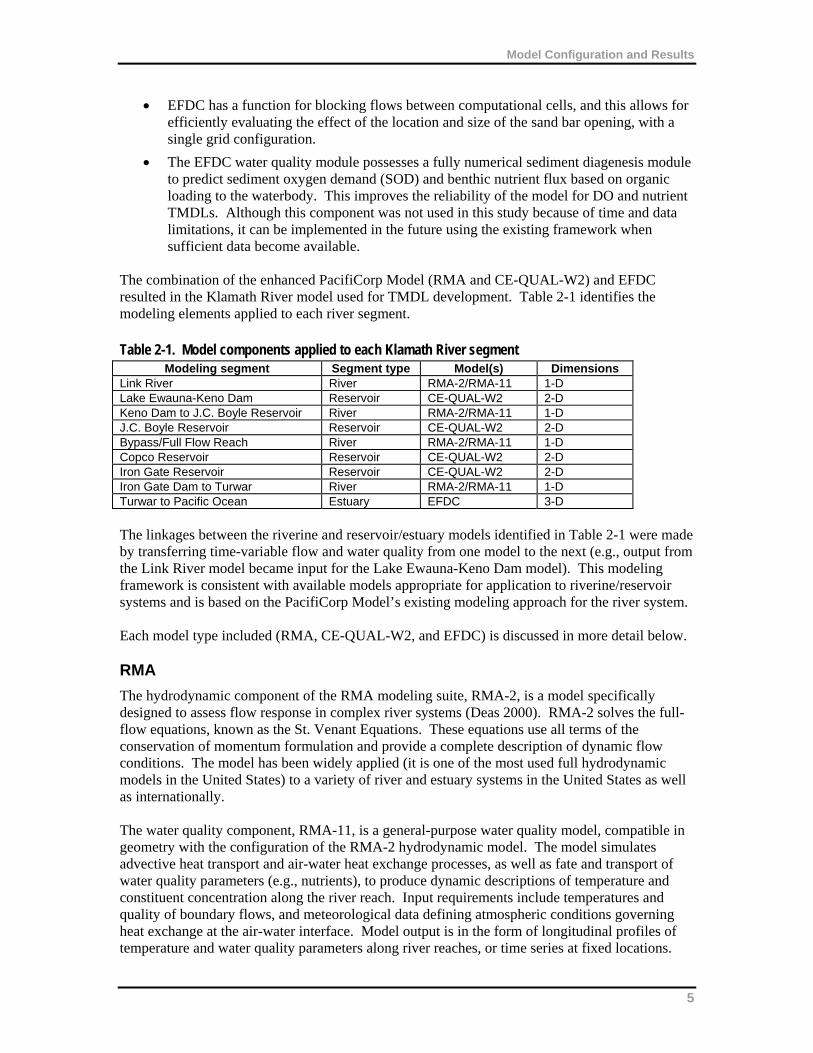
The combination of the enhanced PacifiCorp Model (RMA and CE-QUAL-W2) and EFDC resulted in the Klamath River model used for TMDL development. Table 2-1 identifies the modeling elements applied to each river segment. Table 2-1. Model components applied to each Klamath River segment
Modeling segment Segment type Model(s) Dimensions Link River River RMA-2/RMA-11 1-D Lake Ewauna-Keno Dam Reservoir CE-QUAL-W2 2-D Keno Dam to J.C. Boyle Reservoir River RMA-2/RMA-11 1-D J.C. Boyle Reservoir Reservoir CE-QUAL-W2 2-D Bypass/Full Flow Reach River RMA-2/RMA-11 1-D Copco Reservoir Reservoir CE-QUAL-W2 2-D Iron Gate Reservoir Reservoir CE-QUAL-W2 2-D Iron Gate Dam to Turwar River RMA-2/RMA-11 1-D Turwar to Pacific Ocean Estuary EFDC 3-D
The linkages between the riverine and reservoir/estuary models identified in Table 2-1 were made by transferring time-variable flow and water quality from one model to the next (e.g., output from the Link River model became input for the Lake Ewauna-Keno Dam model). This modeling framework is consistent with available models appropriate for application to riverine/reservoir systems and is based on the PacifiCorp Model’s existing modeling approach for the river system. Each model type included (RMA, CE-QUAL-W2, and EFDC) is discussed in more detail below. RMA
The hydrodynamic component of the RMA modeling suite, RMA-2, is a model specifically designed to assess flow response in complex river systems (Deas 2000). RMA-2 solves the full-flow equations, known as the St. Venant Equations. These equations use all terms of the conservation of momentum formulation and provide a complete description of dynamic flow conditions. The model has been widely applied (it is one of the most used full hydrodynamic models in the United States) to a variety of river and estuary systems in the United States as well as internationally. The water quality component, RMA-11, is a general-purpose water quality model, compatible in geometry with the configuration of the RMA-2 hydrodynamic model. The model simulates advective heat transport and air-water heat exchange processes, as well as fate and transport of water quality parameters (e.g., nutrients), to produce dynamic descriptions of temperature and constituent concentration along the river reach. Input requirements include temperatures and quality of boundary flows, and meteorological data defining atmospheric conditions governing heat exchange at the air-water interface. Model output is in the form of longitudinal profiles of temperature and water quality parameters along river reaches, or time series at fixed locations.
5
Model Configuration and Results
CE-QUAL-W2
The U.S. Army Corps of Engineers’ CE-QUAL-W2 is a 2-D, longitudinal/vertical (laterally averaged), hydrodynamic and water quality model (Cole and Wells, 2003). The model allows for application to streams, reservoirs, and estuaries with variable grid spacing, time-variable boundary conditions, and multiple inflows and outflows from point/nonpoint sources and precipitation. The two major components of the model include hydrodynamics and water quality kinetics, which simulate changes in constituent concentrations. Both of these components are coupled (i.e., the hydrodynamic output is used to drive the water quality at every timestep). The hydrodynamic portion of the model predicts water surface elevations, velocities, and temperature. The ULTIMATE-QUICKEST numerical scheme used in the CE-QUAL-W2 model is designed to reduce the numerical diffusion in the vertical direction to a minimum and in areas of high gradients, reduce the undershoots and overshoots that could produce small negative concentrations. The water quality kinetics portion can simulate 21 water quality parameters including DO, nutrients, phytoplankton interactions, and pH. EFDC
EFDC is a general purpose modeling package for simulating 1-D, 2-D, and 3-D flow, transport, and biogeochemical processes in surface water systems including rivers, lakes, estuaries, reservoirs, wetlands, and coastal regions. The EFDC model was originally developed at the Virginia Institute of Marine Science for estuarine and coastal applications. This model is now being supported by EPA and has been used extensively to support TMDL development throughout the country. In addition to hydrodynamic, salinity, and temperature transport simulation capabilities, EFDC is capable of simulating cohesive and non-cohesive sediment transport, near-field and far-field discharge dilution from multiple sources, eutrophication processes, the transport and fate of toxic contaminants in the water and sediment phases, and the transport and fate of various life stages of finfish and shellfish. Cohesive sediment refers to silt and clay particles while non-cohesive refers to anything larger than silt (e.g., sand, gravel). The EFDC model has been extensively tested, documented, and applied to environmental studies worldwide by universities, governmental agencies, and environmental consulting firms. The structure of the EFDC model includes four major modules: (1) a hydrodynamic model, (2) a water quality model, (3) a sediment transport model, and (4) a toxics model. The water quality portion of the model simulates the spatial and temporal distributions of 22 water quality parameters including DO, suspended algae (3 groups), attached algae, various components of carbon, nitrogen, phosphorus and silica cycles, and fecal coliform bacteria. Salinity, water temperature, and total suspended solids are needed for computation of the 22 water quality parameters, and they are simulated by the hydrodynamic model. EFDC’s water quality model also includes a sediment process model, which uses a slightly modified version of the Chesapeake Bay 3-D model (Park et al. 1995). Upon receiving the particulate organic matter (OM) deposited from the overlying water column, it simulates its diagenesis and the resulting fluxes of inorganic substances (ammonium, nitrate, phosphate and silica) and SOD back to the water column. The coupling of the sediment process model with the water quality model not only enhances the model's predictive capability of water quality parameters, but also enables it to simulate the long-term changes in water quality conditions in response to changes in nutrient loads.
6
Model Configuration and Results
2.2 Model Enhancements
Although the original PacifiCorp Model (Watercourse Engineering, Inc. 2004) is capable of addressing the identified water quality issues, a number of enhancements to the model were necessary to expedite and strengthen the model for the rigors of TMDL development for the Klamath River. Selected algorithms in the PacifiCorp Model were considered for augmentation of the modeling framework to address specific processes and support TMDL development. Enhancements were made in the following areas:
BOD/OM unification
Two-state algae transformation algorithm in Lake Ewauna
Monod-type continuous SOD and OM decay
pH simulation in RMA
OM-dependent light extinction simulation in RMA
Reaeration formulations
Dynamic OM partitioning
Periphyton carrying capacity
Additional shading in RMA
Second order polynomial spillway representation
2.2.1 BOD/OM Unification
It was determined that biochemical oxygen demand (BOD) should not be modeled in addition to OM because BOD itself is a surrogate for OM. The BOD compartment in the modeling system was eliminated for both the riverine (RMA model component) and reservoir (CE-QUAL-W2 model component) sections. To maintain consistency between the new version of the model and the original version in terms of organic loading, the BOD concentration in the original version was converted to an OM component by using a stoichiometric ratio of BOD:OM = 1.4. This stoichiometric coefficient was derived on the basis of the original RMA-11 model and is also consistent with representation in the CE-QUAL-W2 model. This converted OM was combined with the OM in the original version to form the total OM in the new version. This conversion allowed the model to represent consistent amounts of OM in the original and new versions. Additionally, in the original CE-QUAL-W2 models for the reservoirs, particulate OM was not included in the tributary boundary condition files. This is expected to result in an underestimation of particulate OM into the system. Therefore, for the major tributaries that are highly productive, such as the Lost River Diversion Channel, particulate OM loading was represented on the basis of data and appropriate assumptions. Concentration boundary condition files were modified using a labile particulate OM (LPOM) to labile dissolved OM (LDOM) ratio of 4.0 (LPOM:LDOM = 0.8:0.2), which is same as for the Link River boundary condition. Labile OM refers to the portion that is decomposed relatively quickly. The state variable slots in the CE-QUAL-W2 models for labile OM (i.e., LDOM and LPOM) were used to represent all dissolved OM and particulate OM, respectively. Therefore, even though the terms “LDOM” and “LPOM” are used when referring to model results, the values essentially represent all OM, without differentiating between labile and refractory components.
7
Model Configuration and Results
2.2.2 Two-state Algae Transformation Algorithm in Lake Ewauna
Very low levels of phytoplankton were observed in lower Lake Ewauna, as shown in the year 2000 monitoring data for the Highway (Hwy) 66 station. Phytoplankton biomass in Lake Ewauna also shows significant variability from upstream (Miller Island water quality station) to downstream (Hwy 66 water quality station). In addition, observed data show that there was a sharp drop in algae concentration at the Miller Island station during the summer. These phenomena were not predicted by the existing PacifiCorp Model, although it is configured to simulate all algae-DO-nutrient interactions represented in the W2 model code.
Simulated algae biomass in the existing PacifiCorp Model is similar at both locations, and algae concentrations remained high throughout the summer period. This is due to the dominant upstream inflow (from UKL) that causes water to flow quickly from upstream to downstream. The inability to accurately predict the temporal and spatial distribution of phytoplankton has significant implications on the water quality dynamics. Therefore, model refinement was needed to better represent the algae dynamics in this lake.
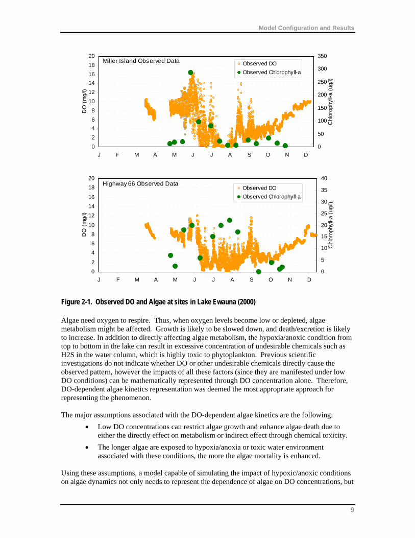
It appears that with the existing kinetic structure in the model, it is not possible to reproduce this type of spatial distribution of algae biomass. During the model testing process, which is described later in this report, the algae growth and mortality parameters were varied significantly in an attempt to reproduce the observed spatial algae pattern in Lake Ewauna. Regardless of the parameter combinations used, the model predicted similar algae magnitudes and patterns at the Miller Island and Hwy 66 stations (due in large part to the rapid transport of algae in Lake Ewauna). It is believed that the summer hypoxia/anoxia in the lake influences the spatial variability of algae biomass in Lake Ewauna. Data show that sometimes during the summer, the entire Lake Ewauna water column becomes hypoxic (exhibiting very low DO concentrations), and even anoxic (exhibiting DO concentrations near zero). Figure 2-1 shows the observed DO data, along with chlorophyll a, at the Miller Island and Hwy 66 locations for 2000 (at approximately 1 meter from the surface). Algal mortality has been causally linked with low DO in UKL (National Research Council 2004) and found to be related to anoxic conditions in other systems (Baric et al. 2003). Available data show no other explanation for the observed phenomenon.
This space intentionally left blank
8
Model Configuration and Results
Miller Island Observed Data
0
2
4
6
8
10
12
14
16
18
20
J F M A M J J A S O N D
DO
(m
g/l)
0
50
100
150
200
250
300
350
Chl
orop
hyll-
a (u
g/l)
Observed DO
Observed Chlorophyll-a
Highway 66 Observed Data
0
2
4
6
8
10
12
14
16
18
20
J F M A M J J A S O N D
DO
(m
g/l)
0
5
10
15
20
25
30
35
40
Chl
orop
hyll-
a (u
g/l)
Observed DO
Observed Chlorophyll-a
Figure 2-1. Observed DO and Algae at sites in Lake Ewauna (2000) Algae need oxygen to respire. Thus, when oxygen levels become low or depleted, algae metabolism might be affected. Growth is likely to be slowed down, and death/excretion is likely to increase. In addition to directly affecting algae metabolism, the hypoxia/anoxic condition from top to bottom in the lake can result in excessive concentration of undesirable chemicals such as H2S in the water column, which is highly toxic to phytoplankton. Previous scientific investigations do not indicate whether DO or other undesirable chemicals directly cause the observed pattern, however the impacts of all these factors (since they are manifested under low DO conditions) can be mathematically represented through DO concentration alone. Therefore, DO-dependent algae kinetics representation was deemed the most appropriate approach for representing the phenomenon. The major assumptions associated with the DO-dependent algae kinetics are the following:
Low DO concentrations can restrict algae growth and enhance algae death due to either the directly effect on metabolism or indirect effect through chemical toxicity.
The longer algae are exposed to hypoxia/anoxia or toxic water environment associated with these conditions, the more the algae mortality is enhanced.
Using these assumptions, a model capable of simulating the impact of hypoxic/anoxic conditions on algae dynamics not only needs to represent the dependence of algae on DO concentrations, but
9
Model Configuration and Results
it needs to track the duration of exposure of algae to these conditions. For example, a cluster of algae in Link River (before entering hypoxic Lake Ewauna) is free of the effects of low DO concentrations. However, after this cluster enters Lake Ewauna, it is subjected to local hypoxic conditions (while being transported downstream). The effect of the hypoxic/anoxic conditions on the algae becomes more severe with distance downstream because the exposure time to these conditions increases. This exposure time is hereby referred to as ET, and it is not the same as the time that the DO is hypoxic/anoxic at a specific location, which is referred to as THA. CE-QUAL-W2, like most numerical hydrodynamic and water quality models, is based on the Eulerian system that does not track the history of travel of particles. Therefore, it is very difficult to directly track the ET of a specific cluster of algae. The PacifiCorp Model was unable to reproduce the sharp algae decline from upstream to downstream in Lake Ewauna, in part because it was unable to consider exposure time. In this study, a two-state algae transformation approach was applied to the model as a surrogate for representing the effect of the ET. The approach involves defining two states of algae, where one state represents the healthy group which is free of the hypoxic/anoxic impact and the other state represents the unhealthy group (for which the physiological condition is severely disturbed because of hypoxia/anoxia). The healthy group is represented using typical algae growth and respiration rates; however, the unhealthy algae growth and respiration rates are very low or 0.0 (because of the hypoxic/anoxic condition’s effect on the algae’s physiology). The ET is indirectly represented through conversion of healthy algae to unhealthy algae using a first-order transformation mechanism when the algae are in the presence of low-DO conditions. The longer the algae are exposed to hypoxia/anoxia, the higher the fraction of algae transformed into the unhealthy state becomes. Thus, the overall growth and respiration rate of the entire algae cluster is reduced because of the larger amount of unhealthy algae. In the following equations, A denotes the healthy group and B denotes the unhealthy group:
BAAA CKCKL
dt
dC21 (1)
BABB CKCKL
dt
dC21 (2)
where CA = concentration of algae group A CB = concentration of algae group B LA = total sources and sinks including kinetics for algae group A as represented in the original model LB = total sources and sinks including kinetics for algae group B as represented in the original model K1= transformation rate from algae group A to B K2 = recovering rate from algae group B to A
This space intentionally left blank
10
Model Configuration and Results
11
The effect of low DO on the kinetic parameters K1 and K2 is represented as:
DOHDO
HDOKK
1
1)0(11 (3)
DOHDO
DOKK
2)0(22 (4)
where K1(0) = the base transformation rate from algae group A to B K2(0) = the base recovering rate from algae group B to A DO = the DO concentration in the water column HDO1 = the half saturation coefficient in mg oxygen /L for K1 HDO2 = the half saturation coefficient in mg oxygen/L for K2
The mechanisms described in Equations (1) through (4) were incorporated into the CE-QUAL-CE-QUAL-W2 source code. The model was then run for Lake Ewauna, and the results indicated that the model was capable of explaining the observed algae patterns reasonably well. It should be noted that the assumptions, mathematical formulations, and code development for algae kinetics are based on general scientific knowledge of algae metabolism. It is recommended that further research be conducted to investigate the impact and response relationships among DO, water chemistry changes, and algae metabolism to better understand this complex phenomenon.
2.2.3 Monod-Type SOD and OM Decay
The PacifiCorp Model used the CE-QUAL-W2 code, which represents SOD and OM decay as a delta function. With the delta function, the SOD and OM decay are activated when DO is greater than a pre-specified value (generally close to zero), and deactivated when DO is lower than the value. This leads to abruptly turning SOD and OM decay on and off when DO is low or fluctuates around the pre-specified value. A Monod-type continuous SOD and OM decay formulation was thus incorporated into the CE-QUAL-W2 code to represent a smoother transition of SOD and OM decay effects when DO is low.
where SOD = effective SOD (g O2/m
2/day) DO = DO concentration in the water column for Kd, or in the bottom water for SOD (milligrams per liter [mg/L]) HDO = half saturation DO concentration (mg/L) SODs = SOD before being adjusted by the water column DO (g O2/m
2/day)
sSOD
HDODO
DOSOD
sKd
HDMDO
DOKd
Model Configuration and Results
Kd = effective OM decay rate (1/day) HDM = half saturation DO concentration for OM decay rate adjustment (mg/L) Kds = OM decay rate before DO adjustment (1/day)
2.2.4 pH Simulation Module in RMA
The standard RMA modeling framework does not have the capability of simulating interactions among nutrients, phytoplankton/benthic algae, and pH. Because pH is a key water quality target for Klamath TMDL development, the modeling framework was enhanced to dynamically simulate pH dynamics. A pH simulation module was developed and incorporated into the RMA framework to simulate the pH in the river, considering the impact of boundary conditions, phytoplankton, periphyton, benthic sources, and atmospheric-water exchange. The state variables for the pH module include Total Inorganic Carbon (TIC) and Alkalinity (Alk). Their transport is simulated using the same algorithms used for transporting other dissolved constituents in RMA. While Alk is assumed to be conservative in the water column, TIC changes due to several physical (water-air interface exchange), chemical (OM decay and benthic sources), and biological (phytoplankton and benthic algae metabolism) factors. The mathematical equations for the pH module are based on those described in Chapter 39 of Chapra (1997), and are detailed in Appendix A.
2.2.5 OM-dependent Light Extinction Formulation in RMA
The existing RMA model does not have the capability of representing the effect of OM on light conditions. Thus, it can inaccurately predict periphyton or phytoplankton growth in the presence of OM. OM can reduce sunlight and limit aquatic vegetation growth. An OM-dependent light extinction formulation was developed using the same formulation in the CE-QUAL-W2 model and incorporated into the RMA code to provide a more realistic representation of the system: Ke = Ke’ + OM × KEOM
where Ke = effective light extinction coefficient Ke’ = light extinction coefficient before OM adjustment OM = OM concentration KEOM = light extinction coefficient adjustment factor related to OM concentration
2.2.6 Reaeration Formulation Modification
In the existing RMA-11 model, the flow velocity used for reaeration calculation was forced to be greater than or equal to 0.5 meters per second (m/s). This resulted in excessive reaeration when the flow velocity was actually slower (e.g., during low-flow conditions). A modification was made to this formulation to set the lower bound of the velocity to 0.03 m/s based on Chapra (1997). This modification results in more reasonable DO predictions under low flow, critical conditions. A scaling factor was also introduced into the RMA-11 model to enhance reaeration just downstream of Iron Gate Dam. At this location, the observed summer DO concentration is much
12
Model Configuration and Results
higher than what can be predicted by RMA-11 using the available empirical formulas. In the model, the DO concentration of water exiting Iron Gate Reservoir during the summer is low due to vertical stratification in the reservoir (and thus low DO concentrations at depths from which water is drawn). Significant reaeration is necessary over a very short distance to increase the low DO concentrations to the significantly higher observed concentrations. The RMA-11 formulas, however, are unable to replicate this phenomenon, which is caused by the presence of significant turbulence downstream of Iron Gate Dam. To account for this observed phenomenon, a scaling factor (or multiplier) was introduced into the RMA-11 model. After multiple iterations during model testing, a value of 100.0 was selected. Application of this scaling factor results in a significantly higher coefficient than what is typically used with the RMA-11 formulas, however, it is necessary (and justifiable) to simulate the observed DO concentrations.
2.2.7 Dynamic OM Partitioning
Key updates were made to the original PacifiCorp Model to transfer model results between segments represented using CE-QUAL-W2 and those represented using RMA. Originally, the upstream boundary conditions for a CE-QUAL-W2 reservoir model were based on model results from the upstream riverine RMA model. In RMA all the OM is represented as a lumped parameter, while in W2 they are partitioned into four different components: LPOM, RPOM, LDOM, and RDOM. Therefore, when transferring the RMA OM results to W2, the OM output must be partitioned into the four components for W2. In the existing PacifiCorp Model, a static partitioning ratio of 0.8:0.2 was used to partition the OM into LPOM and LDOM, respectively. This static conversion factor does not account for the change in OM composition that occurs throughout the system. Therefore, a dynamic OM partitioning scheme was implemented that calculates and tracks the time-variable partitioning ratio in the reservoir models and applies the ratios to downstream segments. Using this approach, different ratios are implemented for J.C. Boyle and Copco reservoirs. For J.C. Boyle Reservoir, the OM in the upstream river flow is partitioned in such a way that, on average, LDOM accounts for 62 percent, LPOM 36 percent, RDOM 1 percent, and RPOM 1 percent. For Copco Reservoir, the corresponding values are: 67 percent, 30 percent, 2 percent, and 1 percent. These values demonstrate that the fraction of dissolved OM increases with downstream distance, while the fraction of particulate OM decreases (because of the effect of settling). The percentages noted above are not fixed for all simulations.
2.2.8 Periphyton Carrying Capacity
In the RMA-11 model code used in the PacifiCorp Model, the carrying capacity of periphyton biomass was implemented such that when the simulated periphyton biomass exceeds a prescribed maximum value, the simulated biomass is set to that value. This method of handling the periphyton carrying capacity results in unbalanced nutrient representation in the system. When the simulated biomass exceeds the prescribed maximum value, additional nutrients are not utilized by the periphyton biomass (as they would be should no maximum be set). The PacifiCorp Model predicts that the periphyton biomass remains constant for an extended period of time during the summer. Not only is this unrealistic, but it is equivalent to artificially removing nutrients from the system. A more reasonable way of reflecting the growth limitation when the simulated periphyton approaches the carrying capacity is to relate the growth rate to the biomass itself. Thus growth is depressed when biomass is high, but it has no impact when biomass is low. The formula is:
13
Model Configuration and Results
Ge=Gx(1-C/Cmax) where Ge = effective growth rate of periphyton (day-1) G = growth rate before adjusting for carrying capacity (self-limiting) effects C = periphyton biomass (g/m2) Cmax = periphyton carrying capacity (g/m2) When the periphyton biomass increases, the corresponding effective growth rate decreases. When the biomass reaches the carrying capacity, the effective growth rate becomes 0.0. Since nutrient uptake is coupled with periphyton growth in water quality models, formulating the effect of carrying capacity in this manner guarantees a balanced nutrient budget in the system.
2.2.9 Additional Shading in RMA
Temperature simulated by the PacifiCorp Model for the Bypass/Full Flow Reach downstream of J.C. Boyle Reservoir was significantly higher than the observed data. Therefore, during the model testing process one of the most influential factors, the representation of solar radiation, was explored. RMA-11 uses empirical equations to internally calculate solar radiation for the thermal and bio-chemical simulations. These equations are based on longitude, altitude, sunrise and sunset time, and cloud condition. To evaluate whether or not RMA-11 was appropriately estimating solar radiation in this area, the RMA-11-estimated solar radiation was compared to the solar radiation data used in the Copco Reservoir CE-QUAL-W2 model. It was found that the solar radiation estimated using RMA-11 is approximately 20% higher than that used in the Copco Reservoir CE-QUAL-W2 model. This apparent over-estimation of solar radiation likely caused the overprediction of temperature noted above. To account for this discrepancy and to reduce the solar radiation calculated by RMA-11, additional shading was configured in the model. A value of 20% was selected based on the comparison made. To maintain consistency among all the RMA-11 models used for the Klamath River, this 20% additional shading was applied to all RMA-11 models. No changes were necessary for the CE-QUAL-W2 or EFDC models since solar radiation is handled differently for those models and because temperature predictions were not uniformly over- or under-estimated.
2.2.10 Second Order Polynomial Spillway Representation
To support TMDL development, The Klamath River model will not only be used to represent the current condition, but it will be used to represent conditions prior to the creation of Keno Dam. Based on information provided by the U.S. Bureau of Reclamation (USBR), a version of the CE-QUAL-W2 model for Lake Ewauna-Keno Dam was developed to represent the historical presence of Keno Reef (McGlashan and Dean 1913). The approach taken to represent the reef required modification of the CE-QUAL-W2 model code. Specifically, Keno Reef was represented in the model using a second-order spillway equation derived by USBR from historical data. The formulation of the spillway equation is:
This space intentionally left blank
14
Model Configuration and Results
Q=101.265(H-1244.5)2-15.030(H-1244.5)+12.35 where Q = flow rate over Keno Reef (cms) H = water surface elevation (m) 1244.5 = the Keno Reef datum (m).
2.3 Model Configuration
Model configuration involved setting up the model computational grid (bathymetry) using available geometric data, designating the model’s state variables, setting boundary conditions, and setting initial conditions. This section describes briefly the configuration process and key components of the model in greater detail.
2.3.1 Segmentation/Computational Grid Setup
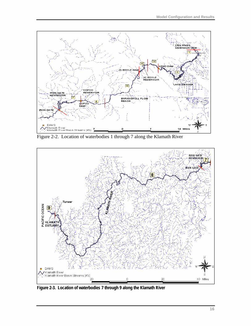
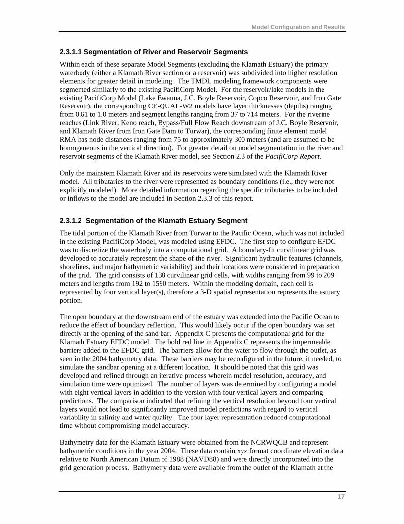
The computational grid setup defines the process of segmenting the entire Klamath River into smaller computational segments for application of the model. In general, bathymetry is the most critical component in developing the grid for the system. The Klamath River model includes the entire Klamath River from Link Dam (at the outlet of the UKL) to the Pacific Ocean. The river is impounded by five dams along its length: Keno, J.C. Boyle, Copco, Copco 2, and Iron Gate Dam. For this modeling study, the Klamath River was divided into nine waterbodies (or Model Segments). Figures 2-2 and 2-3 show each of the waterbodies from upstream to downstream. Note that distances for each waterbody are approximate. Appendix B presents an excerpt (verbatim) from Klamath River Water Quality Model Implementation, Calibration, and Validation (PacifiCorp 2005) that summarizes geometric information for all waterbodies. Each of these waterbodies was represented using unique geometric and hydrological characteristics in the model and is detailed in subsequent sections.
This space intentionally left blank
15
Model Configuration and Results
Figure 2-2. Location of waterbodies 1 through 7 along the Klamath River
Figure 2-3. Location of waterbodies 7 through 9 along the Klamath River
16
Model Configuration and Results
2.3.1.1 Segmentation of River and Reservoir Segments
Within each of these separate Model Segments (excluding the Klamath Estuary) the primary waterbody (either a Klamath River section or a reservoir) was subdivided into higher resolution elements for greater detail in modeling. The TMDL modeling framework components were segmented similarly to the existing PacifiCorp Model. For the reservoir/lake models in the existing PacifiCorp Model (Lake Ewauna, J.C. Boyle Reservoir, Copco Reservoir, and Iron Gate Reservoir), the corresponding CE-QUAL-W2 models have layer thicknesses (depths) ranging from 0.61 to 1.0 meters and segment lengths ranging from 37 to 714 meters. For the riverine reaches (Link River, Keno reach, Bypass/Full Flow Reach downstream of J.C. Boyle Reservoir, and Klamath River from Iron Gate Dam to Turwar), the corresponding finite element model RMA has node distances ranging from 75 to approximately 300 meters (and are assumed to be homogeneous in the vertical direction). For greater detail on model segmentation in the river and reservoir segments of the Klamath River model, see Section 2.3 of the PacifiCorp Report. Only the mainstem Klamath River and its reservoirs were simulated with the Klamath River model. All tributaries to the river were represented as boundary conditions (i.e., they were not explicitly modeled). More detailed information regarding the specific tributaries to be included or inflows to the model are included in Section 2.3.3 of this report.
2.3.1.2 Segmentation of the Klamath Estuary Segment
The tidal portion of the Klamath River from Turwar to the Pacific Ocean, which was not included in the existing PacifiCorp Model, was modeled using EFDC. The first step to configure EFDC was to discretize the waterbody into a computational grid. A boundary-fit curvilinear grid was developed to accurately represent the shape of the river. Significant hydraulic features (channels, shorelines, and major bathymetric variability) and their locations were considered in preparation of the grid. The grid consists of 138 curvilinear grid cells, with widths ranging from 99 to 209 meters and lengths from 192 to 1590 meters. Within the modeling domain, each cell is represented by four vertical layer(s), therefore a 3-D spatial representation represents the estuary portion. The open boundary at the downstream end of the estuary was extended into the Pacific Ocean to reduce the effect of boundary reflection. This would likely occur if the open boundary was set directly at the opening of the sand bar. Appendix C presents the computational grid for the Klamath Estuary EFDC model. The bold red line in Appendix C represents the impermeable barriers added to the EFDC grid. The barriers allow for the water to flow through the outlet, as seen in the 2004 bathymetry data. These barriers may be reconfigured in the future, if needed, to simulate the sandbar opening at a different location. It should be noted that this grid was developed and refined through an iterative process wherein model resolution, accuracy, and simulation time were optimized. The number of layers was determined by configuring a model with eight vertical layers in addition to the version with four vertical layers and comparing predictions. The comparison indicated that refining the vertical resolution beyond four vertical layers would not lead to significantly improved model predictions with regard to vertical variability in salinity and water quality. The four layer representation reduced computational time without compromising model accuracy. Bathymetry data for the Klamath Estuary were obtained from the NCRWQCB and represent bathymetric conditions in the year 2004. These data contain xyz format coordinate elevation data relative to North American Datum of 1988 (NAVD88) and were directly incorporated into the grid generation process. Bathymetry data were available from the outlet of the Klamath at the
17
Model Configuration and Results
Pacific Ocean upstream to the Rt. 101 Bridge (Hwy 101 @ Klamath). No bathymetry data were available from the Rt. 101 Bridge upstream to the USGS Klamath River near Klamath station (USGS 11530500) (a distance of approximately 3,300 meters). To address this data gap, a constant bed slope similar to the upstream portion of the bathymetry data (where the bathymetry was measured) was assumed. This slope was refined until tidal impacts were properly represented (i.e., no tidal effect was observed at Turwar). River bank boundaries for the grid were defined using digital orthophotography obtained from the California Spatial Information Library (CaSIL) (http://gis.ca.gov/). Orthophotography was used instead of USGS quadrangle images due to the age of the USGS quadrangles. For example, the Requa, CA USGS quadrangle was last revised in 1966, while Requa orthophotography represents conditions in 1998. The images were georeferenced to a Universal Transverse Mercator (UTM) Zone 10 projection, using a NAD 1927 horizontal datum. This coordinate system was then used to develop the horizontal dimensions of the grid and calculate the dimensions of the computational cells.
2.3.2 State Variables
Selection of appropriate model state variables to represent water quality processes of concern is a critical factor in model configuration. For this study, state variables were selected to most accurately predict TMDL impairments and related physical, chemical, and biological processes. State variables varied for each model type in the Klamath River model (RMA, CE-QUAL-W2, and EFDC). Note that pH is not a state variable. It is computed from alkalinity and TIC. Alkalinity and TIC are transported by the model and are thus state variables. In addition, TDS was inherited from the PacifiCorp model. No effort was made to remove it since it has no impact on the water quality simulation. The following state variables were configured for the riverine segments of the Klamath River model (for the RMA portions of the model):
1. Arbitrary Constituent (configured as a tracer to evaluate the mass balance) 2. DO 3. Organic matter (OM) 4. Orthophosphorus (PO4) 5. Ammonium (NH4) 6. Nitrite (NO2) 7. Nitrate (NO3) 8. Phytoplankton 9. Temperature 10. Periphyton 11. Total inorganic carbon (TIC) 12. Alkalinity (Alk)
The reservoir segments of the Klamath River, where the CE-QUAL-W2 model was applied, were configured using the following active state variables:
1. Labile dissolved organic matter (LDOM) 2. Refractory dissolved organic matter (RDOM) 3. Labile particulate organic matter (LPOM) 4. Refractory particulate organic matter (RPOM) 5. Inorganic Suspended Solids (ISS) 6. PO4 7. NH4
18
Model Configuration and Results
8. NO2/NO3 9. DO 10. Phytoplankton 11. Alk 12. TIC 13. Temperature 14. Tracer 15. TDS 16. Age (to track detention time at different locations) 17. Coliform bacteria
The estuarine portion of the Klamath River, which was modeled using EFDC, was configured with the following constituents as state variables:
1. Phytoplankton 2. Labile particulate organic carbon (LPOC) 3. Labile dissolved organic carbon (LDOC) 4. Labile particulate organic phosphorous (LPOP) 5. Labile dissolved organic phosphorous (LDOP) 6. PO4 7. Labile particulate organic nitrogen (LPON) 8. Labile dissolved organic nitrogen (LDON) 9. NH4 10. NO2/NO3 11. DO 12. Temperature 13. Salinity 14. Periphyton
The RMA model considers a single, lumped OM constituent while the CE-QUAL-W2 model contains four compartments (LDOM, RDOM, LPOM, and RPOM). Because available data are insufficient to accurately partition between labile and refractory components and because RMA only considers lumped OM, all the OM boundary conditions configured for the reservoir models were partitioned between only dissolved and particulate components. Further partitioning between labile and refractory components was not implemented. It’s important to note that the state variable slots in the CE-QUAL-W2 models for labile OM (i.e., LDOM and LPOM) were used to represent the all dissolved OM and particulate OM, respectively. Therefore, even though the terms “LDOM” and “LPOM” are used when referring to model results, the values essentially represent all OM, without differentiating between labile and refractory components. Because average values are used in the model to represent characteristics such as decay rate, the model can be considered to inherently include some amount of both fast- and slow-decaying OM material (i.e., some amount of labile and refractory material). The model was configured such that a small amount of true refractory OM can be generated through algal metabolism, however, this amount is typically negligible. For the EFDC model of the estuary, the organic nutrients were not partitioned between labile and refractory components either. Rather ,they were lumped together and represented using the labile state variable slots.
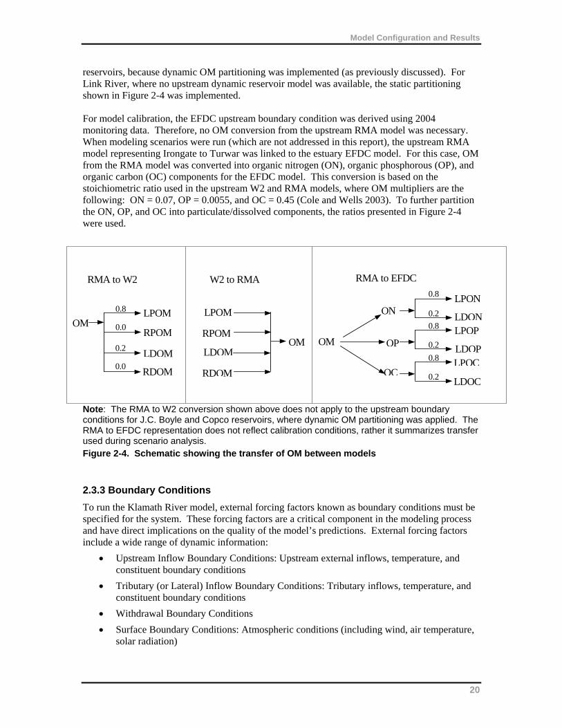
The schematic below (Figure 2-4) shows the flow of OM to and from each of the models. The 0.8:0.2 ratio for partitioning OM was used in the existing PacifiCorp Model and was based on the CE-QUAL-W2 algae partition coefficient (APOM = 0.8). The RMA to W2 conversion shown in Figure 2-4 does not apply to the upstream boundary conditions for J.C. Boyle and Copco
19
Model Configuration and Results
reservoirs, because dynamic OM partitioning was implemented (as previously discussed). For Link River, where no upstream dynamic reservoir model was available, the static partitioning shown in Figure 2-4 was implemented. For model calibration, the EFDC upstream boundary condition was derived using 2004 monitoring data. Therefore, no OM conversion from the upstream RMA model was necessary. When modeling scenarios were run (which are not addressed in this report), the upstream RMA model representing Irongate to Turwar was linked to the estuary EFDC model. For this case, OM from the RMA model was converted into organic nitrogen (ON), organic phosphorous (OP), and organic carbon (OC) components for the EFDC model. This conversion is based on the stoichiometric ratio used in the upstream W2 and RMA models, where OM multipliers are the following: ON = 0.07, OP = 0.0055, and OC = 0.45 (Cole and Wells 2003). To further partition the ON, OP, and OC into particulate/dissolved components, the ratios presented in Figure 2-4 were used.
OM
LPOM
RPOMOM
LPOM
LDOM
0.8
0.0
OM
ON
OP
OC
LPON
LDONLPOP
LDOPLPOC
LDOC
0.8
0.8
0.8
0.2
0.2
0.2
W2 to RMA RMA to W2 RMA to EFDC
RPOM
RDOM
0.2
0.0
LDOM
RDOM
Note: The RMA to W2 conversion shown above does not apply to the upstream boundary conditions for J.C. Boyle and Copco reservoirs, where dynamic OM partitioning was applied. The RMA to EFDC representation does not reflect calibration conditions, rather it summarizes transfer used during scenario analysis. Figure 2-4. Schematic showing the transfer of OM between models
2.3.3 Boundary Conditions
To run the Klamath River model, external forcing factors known as boundary conditions must be specified for the system. These forcing factors are a critical component in the modeling process and have direct implications on the quality of the model’s predictions. External forcing factors include a wide range of dynamic information:
Upstream Inflow Boundary Conditions: Upstream external inflows, temperature, and constituent boundary conditions
Tributary (or Lateral) Inflow Boundary Conditions: Tributary inflows, temperature, and constituent boundary conditions
Withdrawal Boundary Conditions
Surface Boundary Conditions: Atmospheric conditions (including wind, air temperature, solar radiation)
20
Model Configuration and Results
Upstream external inflows essentially represent the inflow at the model’s starting point. Tributary inflows represent the major tributaries that feed into the Klamath River. All water removed from the system is combined within the withdrawals category. The surface boundary conditions are determined by the meteorological or atmospheric conditions and include air temperature, dew point temperature, wind speed, wind direction, and cloud cover. The meteorological file from the original PacifiCorp Model was maintained since it was based on real data and was intensively reviewed. Data obtained from station KFLO near Klamath Falls were used to represent the conditions from Link Dam to J.C. Boyle Dam. Data from Brazie Ranch represent the boundary conditions from J.C. Boyle Dam to Seiad Valley. For the reach from Seiad Valley to Turwar, the weather data from Hoopa and Somes Bar were used to represent the meteorological boundary conditions. Data from the Arcata Eureka Airport were applied to the estuarine portion of the Klamath River (Turwar to the Pacific Ocean), as described later in Section 2.3.3.9. The following subsections provide a detailed description of the boundary conditions used to represent each modeled segment. The descriptions begin upstream at the Link River segment and continue downstream to the Klamath Estuary segment. In the existing PacifiCorp Model, boundary conditions were set as time series at each location on the basis of observed data or other assumptions where data were not available. For periods when no data were available, the model internally estimates the boundary on the basis of linearly interpolating the time series provided in the boundary condition files. In some situations, boundary conditions were updated using more recently acquired monitoring data. Both types of modification are further described in this section. The upper and middle segments of the model (Model Segments 1 through 8) were tested (calibrated) using data from the year 2000. In addition, the calibration of the upper segments (Model Segments 1 through 5) was further corroborated (validated) with observed data for 2002. The estuarine portion (Model Segment 9), which was modeled with EFDC, was calibrated using data from the year 2004. As described in Section 3.0, these periods were selected because of data availability. In subsequent discussions, boundary condition descriptions are first described for the year 2000. Any deviations from the year 2000 representation for the year 2002 are then noted.
2.3.3.1 Model Segment 1: Link River
The Link River segment begins at the outlet of UKL (Link Dam) and ends at Lake Ewauna. Four types of boundary conditions were included in this model segment: upstream inflow boundary conditions, tributary boundary conditions, downstream stage-discharge boundary conditions, and surface boundary conditions (discussed above). Upstream Inflow Boundary Conditions: The inflow to Link River is from UKL through releases from Link Dam. Since there were no observed data available at the head of Link River for 2000, observed water quality data at Pelican Marina (in UKL) were used as the basis for upstream boundary conditions. This representation is different than that in the existing PacifiCorp Model which used multiple year composite data for Link River at Fremont Bridge as the basis of boundary condition. Considering the significant inter-year variability in water quality in UKL, it is preferable to use data collected during the modeling year rather than other years to represent the external forces at boundaries. Monitoring data for NH4, NO2/NO3, phytoplankton, DO, and temperature were directly applied to the boundary conditions using a linear interpolation method
21
Model Configuration and Results
to obtain daily values for dates without data. OM boundary conditions were derived using observed total phosphorus (TP), dissolved PO4, and chlorophyll a data and following these steps:
Step 1: derive algal P as: OPalg = Chla × CCHA / AGP Step 2: derive non-algal P as: OPnon-alg = TP – dissolved PO4 – OPalg Step 3: derive OM as: OM = OPnon-alg × OMP where
Chla = observed chlorophyll a concentration (µg/L) CCHA = 0.067 (mg-algae per µg-chlorophyll a); derivation: Algae = Chla × 67 × (1 mg/1000 ug), where 67 represents the Algae:Chla ratio defined as 30/0.45 (on the basis of the WASP model default ratio of 30 for Algae-C:Chla and the CE-QUAL-W2 model default ratio of 0.45 for Algae-C:Algae) AGP = algal P content coefficient (mg-algae / mg-P) OMP = organic matter P content coefficient (mg-OM / mg-P)
OMP was determined to be 180.0 based on 2002 data for Link River at Fremont Bridge (where the average organic carbon:organic phosphorus ratio is 81, and thus the OM:OP ratio is 81 / 0.45 = 180.0). AGP was assumed to be the same as OMP because phytoplankton is the major source of OM in UKL. BOD was not configured for the model because all OM are represented using a single state variable (as previously noted). Initially, the total PO4 boundary condition was represented using the dissolved PO4 monitoring data at Pelican Marina. It was found, however, that setting the PO4 boundary concentration at Link River to the observed dissolved PO4 value resulted in a significant underprediction of PO4 concentration at Miller Island, in Lake Ewauna. Because Link River flow is dominant in upper Lake Ewauna, the PO4 concentration at Miller Island should be similar in magnitude and pattern to that at the head of Link River. Several model sensitivity analyses confirmed this. The difference between the dissolved PO4 data at Pelican Marina and the PO4 data at Miller Island suggests that the dissolved PO4 at Pelican Marina is likely not a good representation of conditions at the head of Link River. Therefore, the observed PO4 data at Miller Island were used as the basis for configuring the PO4 boundary condition at Link Dam. The alkalinity boundary condition was configured on the basis of alkalinity monitoring data at Link River and Miller Island. In 2000 there was a limited amount of alkalinity data at Link River (on seven discrete dates). These data were insufficient to accurately predict alkalinity concentrations at Miller Island. Therefore, Miller Island data were used to supplement the Link River data in constructing the boundary condition. The first step in doing this was to compare the flow from Link River and the Lost River Diversion Channel to determine the period during which Link River flow was dominant. For this period the alkalinity at Miller Island would be similar in magnitude to that at Link River. Therefore, data at Miller Island were incorporated into the Link River data to form an expanded data set. The upstream boundary condition for alkalinity was then configured using this expanded data set. There were no data available for TIC; therefore, the TIC boundary condition was obtained through the pH calibration process for Miller Island. Initially, TIC at the Link River boundary was derived on the basis of pH at Miller Island and alkalinity at Link River. These estimates were refined to achieve a better calibration of pH at Miller Island in Lake Ewauna. The upstream boundary condition for the 2002 model was derived using a method similar to that used for 2000. Available data at both the head of Link River (Fremont Bridge) and at Pelican
22
Model Configuration and Results
Marina were combined to form a composite data set for 2002 boundary condition derivation. Monitoring data for PO4, NH4, NO2/NO3, phytoplankton, DO, and temperature were directly applied to the boundary conditions using a linear interpolation method to obtain daily values for dates without data. The OM boundary condition was derived using the same approach used for the 2000 model. The alkalinity boundary condition was derived on the basis of monitoring data at Fremont Bridge. And the TIC boundary condition was derived on the basis of alkalinity data and pH data at the same location. Tributary Boundary Conditions: There are two diversions from UKL at Link Dam. These diversions are two powerhouses that discharge water from UKL into the Link River segment (East Side and West Side). USGS gage 11507500 (Link River at Klamath Falls, Oregon) is between the powerhouse discharges. The constituent concentrations for the tributary boundary conditions were set to be the same as the upstream boundary conditions because the powerhouses have the same water source as the upstream boundary (UKL). Downstream Boundary Conditions: Downstream boundary conditions were configured using a stage-discharge relationship. Although this type of boundary condition does not allow for representation of the backflow condition that occasionally occur at the mouth of Link River, it is a better predictive tool than using the Lake Ewauna elevation as the downstream boundary condition. The backflow condition does not have a significant impact on the loading rate from Link River to Lake Ewauna, thus, it does not significantly impact the water quality in the lake.
2.3.3.2 Model Segment 2: Lake Ewauna to Keno Dam
This segment extends from the point where Link River enters Lake Ewauna to the outlet at Keno Dam. Five types of boundary conditions were included in the Klamath River model for the Lake Ewauna segment. They are upstream inflow boundary conditions, tributary boundary conditions, withdrawal boundary conditions, downstream outflow boundary conditions, and surface boundary conditions. Upstream Inflow Boundary Conditions: The upstream boundary condition was defined as the water flowing into Lake Ewauna from Link River (Model Segment 1). Link River’s flow was determined by using the observed flows at USGS flow gage 11507500 plus the flow from the PacifiCorp West Turbine (powerhouse) gage, which is downstream of the USGS gage. The upstream boundary conditions for water quality constituent concentrations were based on the model results in the downstream region of the Link River Model Segment. PO4, NH4, NO2/NO3, DO, phytoplankton, Alk, TIC, and temperature were directly transferred from the RMA-11 model (from Link River) to the CE-QUAL-W2 input data file for Lake Ewauna. Output for OM from Link River was applied to the Lake Ewauna segment and partitioned into four components: LDOM, RDOM, LPOM, and RPOM with partition ratios as 0.2, 0.0, 0.8, and 0.0, respectively. These ratios were based on the CE-QUAL-W2 ALPOM value and the decision not to further partition OM between labile and refractory components. These assumptions were justified because the majority of the organic matter from UKL are likely generated by phytoplankton blooms and metabolism. Therefore, the CE-QUAL-W2 ALPOM value can be used to represent partitioning. In reality significant spatial and temporal variability associated with organic matter composition may exist, however insufficient data are available to more accurately represent the
23
Model Configuration and Results
organic matter boundary conditions. In addition, CE-QUAL-W2 isn’t capable of representing seasonal variability of OM composition for the boundary conditions. Tributary Boundary Conditions: There are 18 definable tributary discharges in the Lake Ewauna to Keno Dam river segment. These discharges include 11 stormwater locations, Columbia Plywood discharge, Klamath Falls Wastewater Treatment Plant, South Suburban Sanitation District, two discharges at Collins Forest Products, Lost River Diversion Channel, and Klamath Straits Drain (KSD). The inflow from the stormwater locations was calculated as an average percentage of total stormwater runoff. The flow from Columbia Plywood was calculated from the discharger’s monthly monitoring reports as an average of 0.01 cubic feet per second (cfs). Variable daily flows were used for the Klamath Falls Wastewater Treatment Plant and ranged from approximately 4 to 12 cfs. Variable daily flows were also used for South Suburban Sanitation District and generally ranged from 1 to 4 cfs. The two discharges at Collins Forest Products had average daily flows of approximately 1.4 cfs and 0.1 cfs. Daily flows from Lost River Diversion Channel and KSD into Lake Ewauna were obtained from USBR’s flow gages at these locations. The water quality constituent concentrations of the tributary boundary conditions were set to be the same as in the previous PacifiCorp Model except for the major tributaries and point sources, including KSD, Klamath Falls Wastewater Treatment Plant, and South Suburban Sanitation District. For these major tributaries and point sources, available data for 2000 and 2002 were used to update the boundary conditions. The details of updating these boundary conditions are summarized as follows: a) KSD The concentration boundary condition at KSD was represented using data at station Pump F in the KSD. The formulas used to convert observed data to model boundary conditions are listed below. For each constituent notation, the one on the left-hand side corresponds to the model boundary condition, while the one on the right-hand side corresponds to observed data. For parameters not listed, observed values were used directly.
Algae [mg/L] = Chlorophyll a [µg/L] × 0.067, where 0.067 was derived similarly to CCHA for the UKL boundary condition (previously described)
LDOM [mg/L] = (TP [mg/L] – PO4 [mg/L]) × 180.0 × 0.7, where 180.0 was derived similarly to OMP for the UKL boundary condition (previously described), and 0.7 was derived on the basis of 2002 data at KSD (Dissolved TP / TP)
RDOM [mg/L] = 0.0 LPOM [mg/L] = (TP – PO4) × 180.0 × 0.3, where the ratio 0.3 was derived from (1.0–
0.7, where 0.7 represents LDOM). RPOM [mg/L] = 0.0 ISS [mg/L] = TSS [mg/L] TIC [mg/L] = f(Alk, temperature, pH), where f represents the functional form relating
TIC to Alkalinity [mg/L], temperature [oC], and pH. Detailed equations can be found in Chapra 1997.
This space intentionally left blank
24
Model Configuration and Results
b) Klamath Falls Wastewater Treatment Plant and South Suburban Sanitation District The water quality constituent concentrations for both the Klamath Falls Wastewater Treatment Plant and South Suburban Sanitation District were set to be the same as in the previous PacifiCorp Model, except for where more recent facility discharge monitoring report data were available. The formulas used to derive the boundary conditions based on data are as follows:
BODu [mg/L] = BOD5 [mg/L] × 3.386, where the ratio 3.386 is based on the assumption that the treatment plants provide secondary treatment, thus the BOD has a decay rate around 0.07/day (Chapra, 1997)
LDOM [mg/L] = BODu / 1.4 × 0.2, where the ratio 1.4 is based on the W2 stoichiometric ratio, and 0.2 is the same as that used for the UKL boundary condition
LPOM [mg/L] = BODu / 1.4 × 0.8, where the ratio 1.4 is based on the W2 stoichiometric ratio, and 0.8 is the same as that used for the UKL boundary condition
OM [mg/L] = LPOM + LDOM, which is based on the conservative assumption that all OM are labile for boundary inputs
ISS [mg/L] = TSS [mg/L] PO4 [mg/L] = TP [mg/L] – BODu / 1.4 / 180.0 Org-P [mg/L] = OM × 0.0055, where the coefficient 0.0055 is the stoichiometric ratio
used in the model TP [mg/L] = Org-P + PO4 Org-N [mg/L] = OM × 0.07 where the coefficient 0.07 is the stoichiometric ratio used in
the model TN [mg/L] = Org-N + NH4 [mg/L] + NO2/NO3 [mg/L]
The 2000 boundary conditions for LDOM, LPOM, and DO at the Klamath Falls Wastewater Treatment Plant were updated using data from 2000. No data were available for ISS, PO4, or NH4 for 2000, therefore data from 2002 were used for the 2000 model. For the 2002 model, LDOM, LPOM, DO, ISS, PO4 and NH4 were all based on the 2002 data. The 2000 and 2002 boundary conditions for LDOM, LPOM, DO, ISS, PO4, and NH4 at South Suburban Sanitation District were configured based on data available for the corresponding year. For dates when PO4 data were not available and thus could not be directly applied, PO4 was derived based on the TP and BOD data using the formulas listed above. Withdrawal Boundary Conditions: Three withdrawals in this segment are explicitly represented, including the Lost River, North Canal, and ADY Canal. Daily flows at all three of these withdrawals are gaged by USBR. There is a lack of available daily withdrawal rates for a few non-USBR irrigation diversions, therefore they are not explicitly represented. Water diversion is grossly represented in the distributed flow, which was derived through a flow balance analysis. The hourly flow rate at Keno Dam was available from USGS gage 11509500 (Klamath River near Keno, Oregon). The flows ranged from less than 500 cfs to more than 4,000 cfs. All these boundary conditions were kept the same as in the previous PacifiCorp Model. Downstream Outflow Boundary Conditions: For Lake Ewauna, the downstream boundary condition was set as the outflow at the point before entering Keno Reach (Keno Dam to J.C.
25
Model Configuration and Results
Boyle Reservoir). The downstream boundary condition was set to be outflow; therefore, no water quality concentration boundary condition was needed.
2.3.3.3 Model Segment 3: Keno Dam to J.C. Boyle Reservoir (Keno Reach)
There were three types of boundary conditions included in this section of the model: upstream inflow boundary conditions, downstream outflow boundary conditions, and surface boundary conditions. Upstream Inflow Boundary Conditions: The upstream inflow to this reach for the 2000 and 2002 models is based on the outflow from Lake Ewauna for the corresponding year. This segment was dominated by upstream water quality, therefore the simulated loading time series for phytoplankton, temperature, PO4, NH4, NO2/NO3, DO, TIC, and Alk from the Lake Ewauna to Keno Dam segment were applied. The four OM constituents predicted by the CE-QUAL-W2 model were combined into one OM constituent and applied to the boundary conditions (as previously discussed). Downstream Outflow Boundary Conditions: Hydrodynamic downstream boundary condition was set as a stage-discharge relationship, which represents the downstream flow as only outflow; therefore, no concentration boundary condition was needed.
2.3.3.4 Model Segment 4: J.C. Boyle Reservoir
The J.C. Boyle Reservoir extends from the J.C. Boyle headwaters (Keno Reach to J.C Boyle Reservoir) to the J.C. Boyle Dam. There were four types of boundary conditions included in this portion of the model. They are upstream inflow boundary conditions, tributary boundary conditions, downstream outflow boundary conditions, and surface boundary conditions. Upstream Inflow Boundary Conditions: Klamath River inflow for the 2000 and 2002 models to J.C. Boyle dam is represented by discharge from the Keno Reach during the corresponding year. The upstream boundary conditions for water quality constituents were based on the model results at the downstream node of the Keno Reach portion of the model for the corresponding year. PO4, NH4, NO2/NO3, DO, phytoplankton, temperature, TIC, and Alk were directly transferred from the RMA-11 model results for Keno Reach to the CE-QUAL-W2 input data file for J.C. Boyle Reservoir. Output for OM from the Keno Reach model was applied to the J.C. Boyle Reservoir (see Section 2.2.1) and was partitioned into four components: LDOM, RDOM, LPOM, and RPOM. The aforementioned dynamic partitioning scheme was applied. This scheme uses the LDOM, RDOM, LPOM, and RPOM fractions derived from model results from the last segment of Keno Reservoir to partition the OM into the four components. Tributary Boundary Conditions: There is one tributary to J.C. Boyle Reservoir, Spencer Creek. Spencer Creek has very limited inflow information. Therefore, it is not configured as a separate tributary in this model. The minor contribution of flow from Spencer Creek is lumped into the upstream headwater in the original PacifiCorp Model, and directly adopted in the TMDL model. The net reservoir accretion/depletion was calculated through a flow balance process aiming to reproduce the observed surface water elevation in the reservoir. This accretion/depletion was configured as a distributed tributary boundary condition in the model. The concentration of the tributary inflow was set to be the same as in the upstream boundary condition.
26
Model Configuration and Results
Downstream Outflow Boundary Conditions: The outflow from the reservoir was calculated as the sum of all recorded releases to the four outlets in the reservoir (powerhouse canal, dam spillway, bypass releases, and fish ladder releases). The downstream boundary condition was set to be outflow; therefore, no concentration boundary condition was needed.
2.3.3.5 Model Segment 5: Bypass/Full Flow Reach
The Bypass/Full Flow Reach extends from the J.C. Boyle Dam to the headwaters of Copco Reservoir. There were four types of boundary conditions included in this portion of the model: upstream inflow boundary conditions, tributary boundary conditions, downstream outflow boundary conditions, and surface boundary conditions. Upstream Inflow Boundary Conditions: There are two inflows to the Bypass/Full Flow Reach. They are releases from J.C. Boyle Dam directly to the Klamath River and the J.C. Boyle Powerhouse tailrace. Measured releases from the dam for 2000 and 2002 were obtained from PacifiCorp and used to represent both inflows for the model for the corresponding years. For the upstream water quality constituent concentration boundary conditions, the simulated loading time series for phytoplankton, temperature, PO4, NH4, NO2/NO3, and DO from the J.C. Boyle Reservoir were applied. The four OM constituents predicted by the CE-QUAL-W2 model were combined into one OM constituent as applied in the Keno Reach boundary condition. Tributary Boundary Conditions: There are no major tributaries, but there are three springs represented by a constant flow of 75 cfs each. The flow rate, temperature, DO, and phytoplankton boundary conditions for the springs were the same as in the original PacifiCorp Model, while the concentrations for the major nutrients (i.e., PO4, NH4, and NO2/NO3) were derived through model calibration. After several iterations, the concentrations for NH4, NO2/NO3, and PO4 were determined to be 0.029 mg/L, 0.25 mg/L, and 0.066 mg/L, respectively. OM concentrations were assumed to be a small value of 0.5 mg/L considering the springs are mainly groundwater. These concentrations were applied to both the 2000 and 2002 models for this reach. Downstream Outflow Boundary Conditions: The downstream boundary condition for the Bypass/Full Flow Reach was configured as a stage-discharge relationship. No concentration boundary condition was needed for the downstream boundary conditions because only outflow exists there.
2.3.3.6 Model Segment 6: Copco Reservoir
The Copco Reservoir model segment extends from Copco Reservoir’s headwaters to Copco Dam. Four types of boundary conditions were included in the portion of the model for Copco Reservoir. They are upstream inflow boundary conditions, tributary boundary conditions, downstream outflow boundary conditions, and surface boundary conditions. Upstream Inflow Boundary Conditions: The inflow for Copco Reservoir was represented as the sum of the inflow into the reservoir and the estimated accretion/depletion for the reservoir. The flows from Bypass/Full Flow Reach were used as inflow to the Copco Reservoir because there are no flow data available at the headwaters of Copco Reservoir. The daily accretion/depletion
27
Model Configuration and Results
was the sum of the daily change in storage in the Copco reservoir and the daily average outflow from the reservoir (minus the daily average inflows from Bypass/Full Flow Reach) as derived in the original PacifiCorp Model. The upstream water quality constituent concentration boundary conditions were based on the model results at the downstream node of the Bypass/Full Flow Reach portion of the model. PO4, NH4, NO2/NO3, DO, phytoplankton, and temperature were directly transferred from the RMA-11 model results for Bypass/Full Flow Reach to the CE-QUAL-W2 input data file for Copco Reservoir. Output for OM from the Bypass/Full Flow Reach portion of the model was applied to Copco Reservoir (see Section 2.2.1) and is partitioned into four components: LDOM, RDOM, LPOM, and RPOM using the dynamic-partitioning approach as described above. Tributary Boundary Conditions: The concentrations of the distributed tributary boundary conditions were set to be the same as the upstream concentration boundary condition in the same manner as in the original model. Downstream Outflow Boundary Conditions: The two main outlets for the Copco Dam are a spillway and two waterway intakes at the Copco powerhouse (treated as a single outlet). Hourly outflow data for the powerhouse and the spillway were available from PacifiCorp and used as reservoir outflow flows. The downstream boundary condition was set to be outflow; therefore, no concentration boundary condition was needed.
2.3.3.7 Model Segment 7: Iron Gate Reservoir
The Iron Gate Reservoir model segment extends from the headwaters of the Iron Gate Reservoir to Iron Gate Dam. Five types of boundary conditions were included in the portion of the model for Iron Gate Reservoir. They are upstream inflow boundary conditions, tributary boundary conditions, withdrawal boundary conditions, downstream outflow boundary conditions, and surface boundary conditions. Upstream Inflow Boundary Conditions: There is no gage to measure inflow to Iron Gate Reservoir; therefore, the flows from the Copco Reservoir were used to represent inflow. Simulated water quality outflow values from Copco Reservoir were applied as the Iron Gate Reservoir inflow water quality constituent concentration boundary conditions, and they were the same configuration as for Lake Ewauna. Tributary Boundary Conditions: There are three tributaries to the Iron Gate Reservoir. They are Camp Creek, Jenny Creek, and Fall Creek. Limited flow information was available for these creeks. The hourly accretion/depletion for the reservoir was calculated as the sum of the daily inflow, outflow, and change in storage in Iron Gate Reservoir. Jenny Creek was represented by this accretion/depletion, as in the original PacifiCorp Model. Neither Camp Creek nor Fall Creek were explicitly configured with contributions in the model. Tributary boundary conditions were not changed from the original PacifiCorp Model. Since Jenny Creek is represented as an accretion/depletion flow, its water quality is represented using the upstream inflow concentrations. This follows the same assumptions as for the upstream reservoirs. Withdrawal Boundary Conditions: The dam’s spillway was modeled as a withdrawal because it draws water to the side of the dam, not over or through the dam. Representing the spillway as a
28
Model Configuration and Results
withdrawal more accurately represents the system. If the spillway were represented as a spillway in W2, water would flow to the end of the reservoir instead of the side, and this can affect the hydrodynamic simulation. Downstream Outflow Boundary Conditions: The Iron Gate dam has four primary outlets: a spillway, penstock, and two fish hatchery intakes. Outflow from the reservoir was based on the outflow in the original PacifiCorp Model. Outflow was determined from PacifiCorp daily flow records for the Powerhouse release and spill and estimates of fish hatchery releases (50 cfs for lower hatchery release and 0 cfs for upper hatchery release). The downstream boundary condition was set to be outflow; therefore, no concentration boundary condition was needed.
2.3.3.8 Model Segment 8: Iron Gate Dam to Turwar
Four types of boundary conditions were included in the portion of the model for Iron Gate Dam to Turwar. They are upstream inflow boundary conditions, tributary boundary conditions, downstream outflow boundary conditions, and surface boundary conditions. Upstream Inflow Boundary Conditions: The upstream inflow boundary conditions for Iron Gate Dam to Turwar were based on PacifiCorp’s original model, which used PacifiCorp’s measured releases from Iron Gate Dam during 2000. Upstream water quality constituent boundary conditions were the simulated outflow values from the Iron Gate reservoir. Tributary Boundary Conditions: There are 23 tributaries to this segment of the Klamath River, including four major tributaries (Shasta, Scott, Salmon, and Trinity rivers). Five tributaries to this reach are actively gauged, including the Shasta, Scott, Salmon, and Trinity rivers, and Indian Creek. Inflows for minor tributaries were defined and quantified as daily accretion/depletions, as in the original PacifiCorp Model. The Scott and Trinity rivers were assigned by summing USGS-gaged flows and daily accretion/depletions. The daily accretion/depletions were determined on the basis of a USGS methodology. Monthly average values were used to determine accretions and depletions for each river segment on the basis of differences in gage readings, and these accretions and depletions were then assigned to individual tributaries according to the estimated basin area. Appendix D presents the USGS methodology for estimating these flows for tributaries (PacifiCorp 2004). Model node and element numbers and type of flow record employed for each tributary are summarized in Table 2-2.
This space intentionally left blank
29
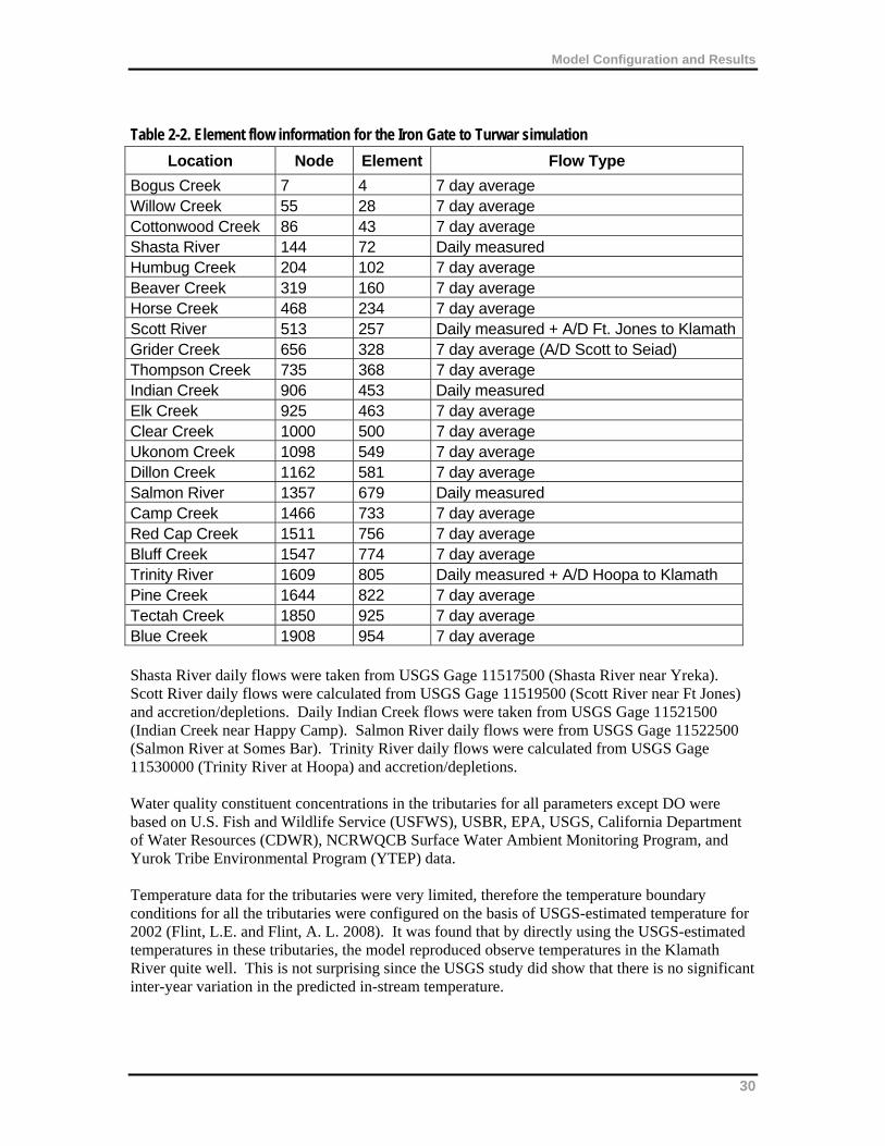
Model Configuration and Results
Table 2-2. Element flow information for the Iron Gate to Turwar simulation
Location Node Element Flow Type
Bogus Creek 7 4 7 day average Willow Creek 55 28 7 day average Cottonwood Creek 86 43 7 day average Shasta River 144 72 Daily measured Humbug Creek 204 102 7 day average Beaver Creek 319 160 7 day average Horse Creek 468 234 7 day average Scott River 513 257 Daily measured + A/D Ft. Jones to KlamathGrider Creek 656 328 7 day average (A/D Scott to Seiad) Thompson Creek 735 368 7 day average Indian Creek 906 453 Daily measured Elk Creek 925 463 7 day average Clear Creek 1000 500 7 day average Ukonom Creek 1098 549 7 day average Dillon Creek 1162 581 7 day average Salmon River 1357 679 Daily measured Camp Creek 1466 733 7 day average Red Cap Creek 1511 756 7 day average Bluff Creek 1547 774 7 day average Trinity River 1609 805 Daily measured + A/D Hoopa to Klamath Pine Creek 1644 822 7 day average Tectah Creek 1850 925 7 day average Blue Creek 1908 954 7 day average Shasta River daily flows were taken from USGS Gage 11517500 (Shasta River near Yreka). Scott River daily flows were calculated from USGS Gage 11519500 (Scott River near Ft Jones) and accretion/depletions. Daily Indian Creek flows were taken from USGS Gage 11521500 (Indian Creek near Happy Camp). Salmon River daily flows were from USGS Gage 11522500 (Salmon River at Somes Bar). Trinity River daily flows were calculated from USGS Gage 11530000 (Trinity River at Hoopa) and accretion/depletions. Water quality constituent concentrations in the tributaries for all parameters except DO were based on U.S. Fish and Wildlife Service (USFWS), USBR, EPA, USGS, California Department of Water Resources (CDWR), NCRWQCB Surface Water Ambient Monitoring Program, and Yurok Tribe Environmental Program (YTEP) data. Temperature data for the tributaries were very limited, therefore the temperature boundary conditions for all the tributaries were configured on the basis of USGS-estimated temperature for 2002 (Flint, L.E. and Flint, A. L. 2008). It was found that by directly using the USGS-estimated temperatures in these tributaries, the model reproduced observe temperatures in the Klamath River quite well. This is not surprising since the USGS study did show that there is no significant inter-year variation in the predicted in-stream temperature.
30
Model Configuration and Results
There were very little to no water quality data available for most tributaries. The only tributaries with sufficient data to represent seasonal variations for 2000 were the Shasta and Scott Rivers (USBR 2003 data). For the other two major rivers, Salmon and Trinity, NCRWQCB derived representative data to approximate the boundary conditions for 2000, based on statistical analysis of historical tributary data. Several historical datasets (1960s to 1980s) with water quality data from CDWR, STORET, USBR, and USGS were supplemented with more recent data (2000 to 2006) from USFWS, USBR, EPA, USGS, CDWR, NCRWQCB, and YTEP. The data were split into two seasonal periods – Wet (November – April) and Dry (May – October), and years which had similar hydrologic conditions to the year 2000 were selected based on statistical measures. The median water quality values for the two seasonal periods were used for boundary conditions. In addition to the USBR data, the NCRWQCB compiled nutrient data for several minor tributaries including Beaver Creek, Bluff Creek, Clear Creek, Dillon Creek, Elk Creek, Red Cap Creek, Indian Creek, and Bogus Creek for the period from 2001 to 2006. These data were divided into two categories. The first was data for Bogus Creek that were used to derive the boundary condition for Bogus Creek. Bogus Creek exhibits significantly higher nutrient concentrations than the other tributaries. The second was data for all other minor tributaries, which were combined to derive values representing all the minor tributaries. Because of a lack of sufficient data to characterize temporal variability, it was deemed appropriate to use an annual average value to represent the boundary conditions from the minor tributaries. DO in all minor tributaries was estimated using 90 percent saturated conditions, except for the Shasta and Scott rivers, where DO data were available. DO saturation concentrations were based on the temperature data and atmospheric pressure corrected for elevation. A detailed description of the boundary conditions for each of the tributaries is provided in Table 2-3.
This space intentionally left blank
31
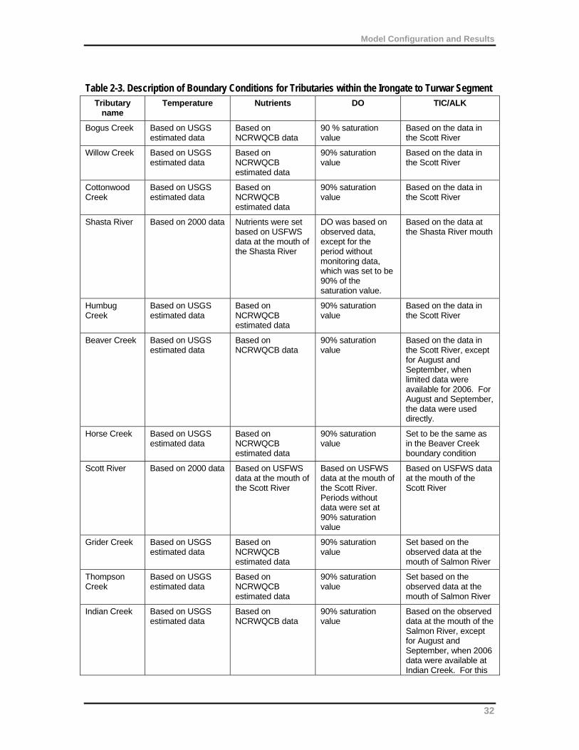
Model Configuration and Results
Table 2-3. Description of Boundary Conditions for Tributaries within the Irongate to Turwar Segment
Tributary name
Temperature Nutrients DO TIC/ALK
Bogus Creek Based on USGS estimated data
Based on NCRWQCB data
90 % saturation value
Based on the data in the Scott River
Willow Creek Based on USGS estimated data
Based on NCRWQCB estimated data
90% saturation value
Based on the data in the Scott River
Cottonwood Creek
Based on USGS estimated data
Based on NCRWQCB estimated data
90% saturation value
Based on the data in the Scott River
Shasta River Based on 2000 data Nutrients were set based on USFWS data at the mouth of the Shasta River
DO was based on observed data, except for the period without monitoring data, which was set to be 90% of the saturation value.
Based on the data at the Shasta River mouth
Humbug Creek
Based on USGS estimated data
Based on NCRWQCB estimated data
90% saturation value
Based on the data in the Scott River
Beaver Creek Based on USGS estimated data
Based on NCRWQCB data
90% saturation value
Based on the data in the Scott River, except for August and September, when limited data were available for 2006. For August and September, the data were used directly.
Horse Creek Based on USGS estimated data
Based on NCRWQCB estimated data
90% saturation value
Set to be the same as in the Beaver Creek boundary condition
Scott River Based on 2000 data Based on USFWS data at the mouth of the Scott River
Based on USFWS data at the mouth of the Scott River. Periods without data were set at 90% saturation value
Based on USFWS data at the mouth of the Scott River
Grider Creek Based on USGS estimated data
Based on NCRWQCB estimated data
90% saturation value
Set based on the observed data at the mouth of Salmon River
Thompson Creek
Based on USGS estimated data
Based on NCRWQCB estimated data
90% saturation value
Set based on the observed data at the mouth of Salmon River
Indian Creek Based on USGS estimated data
Based on NCRWQCB data
90% saturation value
Based on the observed data at the mouth of the Salmon River, except for August and September, when 2006 data were available at Indian Creek. For this
32
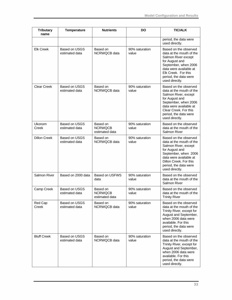
Model Configuration and Results
33
Tributary name
Temperature Nutrients DO TIC/ALK
period, the data were used directly.
Elk Creek Based on USGS estimated data
Based on NCRWQCB data
90% saturation value
Based on the observed data at the mouth of the Salmon River except for August and September, when 2006 data were available at Elk Creek. For this period, the data were used directly.
Clear Creek Based on USGS estimated data
Based on NCRWQCB data
90% saturation value
Based on the observed data at the mouth of the Salmon River, except for August and September, when 2006 data were available at Clear Creek. For this period, the data were used directly.
Ukonom Creek
Based on USGS estimated data
Based on NCRWQCB estimated data
90% saturation value
Based on the observed data at the mouth of the Salmon River
Dillon Creek Based on USGS estimated data
Based on NCRWQCB data
90% saturation value
Based on the observed data at the mouth of the Salmon River, except for August and September, when 2006 data were available at Dillon Creek. For this period, the data were used directly.
Salmon River Based on 2000 data Based on USFWS data
90% saturation value
Based on the observed data at the mouth of the Salmon River
Camp Creek Based on USGS estimated data
Based on NCRWQCB estimated data
90% saturation value
Based on the observed data at the mouth of the Trinity River
Red Cap Creek
Based on USGS estimated data
Based on NCRWQCB data
90% saturation value
Based on the observed data at the mouth of the Trinity River, except for August and September, when 2006 data were available. For this period, the data were used directly.
Bluff Creek Based on USGS estimated data
Based on NCRWQCB data
90% saturation value
Based on the observed data at the mouth of the Trinity River, except for August and September, when 2006 data were available. For this period, the data were used directly.
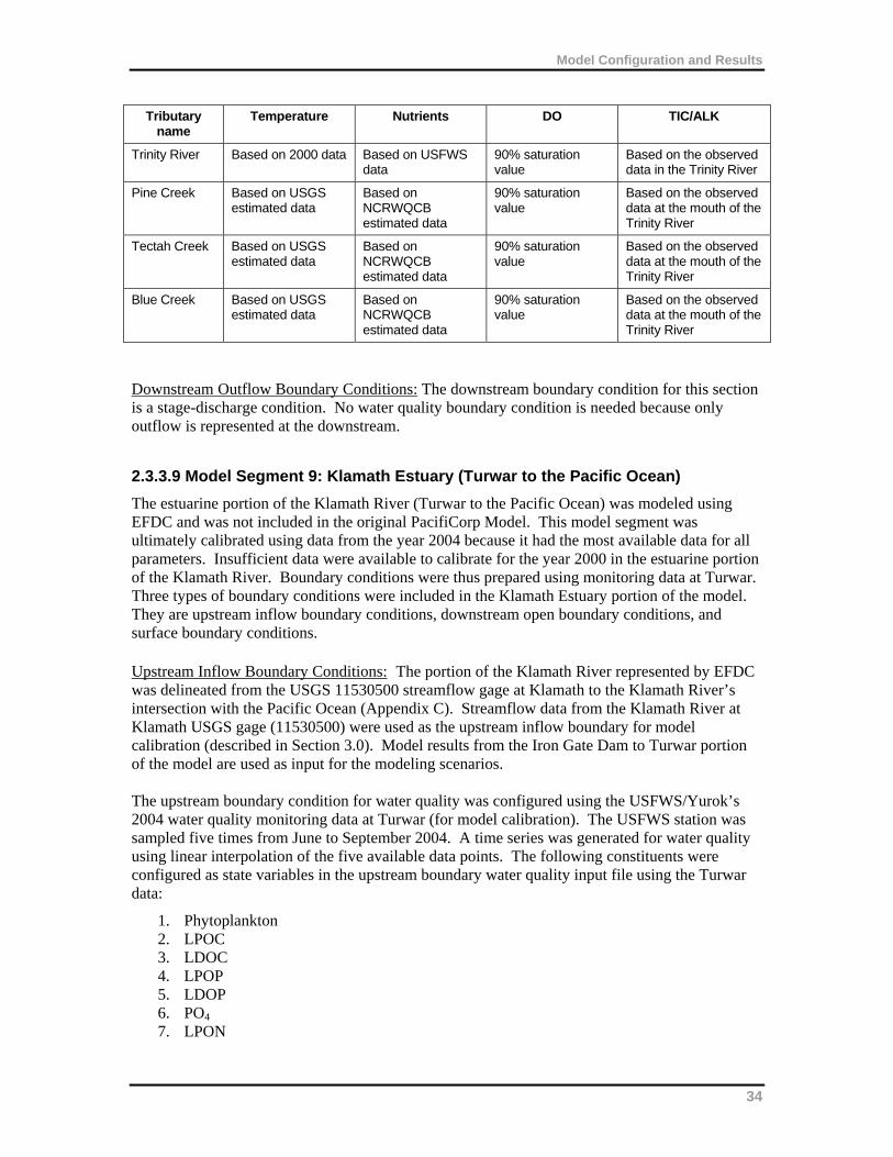
Model Configuration and Results
34
Tributary name
Temperature Nutrients DO TIC/ALK
Trinity River Based on 2000 data Based on USFWS data
90% saturation value
Based on the observed data in the Trinity River
Pine Creek Based on USGS estimated data
Based on NCRWQCB estimated data
90% saturation value
Based on the observed data at the mouth of the Trinity River
Tectah Creek Based on USGS estimated data
Based on NCRWQCB estimated data
90% saturation value
Based on the observed data at the mouth of the Trinity River
Blue Creek Based on USGS estimated data
Based on NCRWQCB estimated data
90% saturation value
Based on the observed data at the mouth of the Trinity River
Downstream Outflow Boundary Conditions: The downstream boundary condition for this section is a stage-discharge condition. No water quality boundary condition is needed because only outflow is represented at the downstream.
2.3.3.9 Model Segment 9: Klamath Estuary (Turwar to the Pacific Ocean)
The estuarine portion of the Klamath River (Turwar to the Pacific Ocean) was modeled using EFDC and was not included in the original PacifiCorp Model. This model segment was ultimately calibrated using data from the year 2004 because it had the most available data for all parameters. Insufficient data were available to calibrate for the year 2000 in the estuarine portion of the Klamath River. Boundary conditions were thus prepared using monitoring data at Turwar. Three types of boundary conditions were included in the Klamath Estuary portion of the model. They are upstream inflow boundary conditions, downstream open boundary conditions, and surface boundary conditions. Upstream Inflow Boundary Conditions: The portion of the Klamath River represented by EFDC was delineated from the USGS 11530500 streamflow gage at Klamath to the Klamath River’s intersection with the Pacific Ocean (Appendix C). Streamflow data from the Klamath River at Klamath USGS gage (11530500) were used as the upstream inflow boundary for model calibration (described in Section 3.0). Model results from the Iron Gate Dam to Turwar portion of the model are used as input for the modeling scenarios. The upstream boundary condition for water quality was configured using the USFWS/Yurok’s 2004 water quality monitoring data at Turwar (for model calibration). The USFWS station was sampled five times from June to September 2004. A time series was generated for water quality using linear interpolation of the five available data points. The following constituents were configured as state variables in the upstream boundary water quality input file using the Turwar data:
1. Phytoplankton 2. LPOC 3. LDOC 4. LPOP 5. LDOP 6. PO4 7. LPON
Model Configuration and Results
8. LDON 9. NH4 10. NO3/NO2 11. DO
Not all data were available to be directly used in the EFDC water quality input file. The following assumptions were made to derive parameters to create the water quality input file:
The particulate to dissolved OM ratio was assumed to be 0.8:0.2. This ratio was also
used to derive the particulate and dissolved components of phosphorus, nitrogen and carbon. It maintains consistency with upstream segments.
Due to a lack of data to further partition OM between labile and refractory components, labile and refractory components were not considered separately.
Organic phosphorous was derived by subtracting PO4 from total phosphorous.
The ON:OM and OP:OM ratios were assumed to be the same as in upstream reaches, which are ON:OM=0.07, and OP:OM=0.0055. These ratios were used to derive ON from OP data.
The algae biomass to chlorophyll ratio was assumed to be 0.067 mg algae/ug Chla, which is the same as those in the upstream reaches.
Diel DO and temperature data were not readily available at the Turwar gage for 2004 when this model was developed. Thus, daily average values were computed on the basis of the diel data for the Upper Estuary monitoring site (at Hwy 101) and specified as the upstream boundary condition at Turwar. The model can be updated to reflect additional monitoring data as these data become available. For modeling scenarios, model output from the Iron Gate Dam to Turwar segment are used. OM conversion from the RMA model to EFDC is presented in Figure 2-4 of Section 2.3.2. Two tributaries to the Klamath Estuary, Hunter Creek and Salt Creek, were also initially considered as part of the boundary conditions but were later eliminated. Flow estimates were available for Hunter Creek, based on drainage area for the period May 1 through September 30, and were found to be relatively insignificant (median value of 5.9 cfs in 2004) in comparison to the Klamath River flows. Salt Creek flows were smaller than those for Hunter Creek. Downstream Open Boundary Conditions: The outlet of the Klamath River at the Pacific Ocean is characterized by a widening of approximately 1,400 meters. Depending on the conditions, the outlet may be largely closed off by a transient sand bar. The opening through this sand bar was set to approximately 200 meters in width for the model, based on measured 2004 bathymetry data. To reduce the influence of boundary reflection, the downstream open boundary of the model was set well into the Pacific Ocean, beyond the physical opening in the sand bar (Appendix C). To allow for flexibility in evaluating the effect of different locations of the sand bar opening, the sand bar is included in the grid system as a column of active cells. It has an internal barrier that blocks the water from penetrating all cells except those representing the opening. Tidal data from the National Oceanic and Atmospheric Administration (NOAA) gage at Crescent City (9419750) were used to represent the tidal boundary of the model. Tidal elevation data from the Crescent City gage are referenced to a mean lower low water (MLLW) vertical datum, while
35
Model Configuration and Results
bathymetry data obtained from the NCRWQCB use the NAVD88. The difference between the two data at this location is approximately 0.38 feet, or 0.116 meters. Tidal elevation data from the Crescent City gage station were adjusted to correspond to the bathymetry datum obtained for the lower portion of the Klamath River. Surface Boundary Conditions: The surface boundary conditions are based on meteorological conditions. The meteorological data required by the EFDC model are specified in two separate files (aser.inp and wser.inp). The aser.inp file is used to specify the atmospheric pressure, air temperature, relative humidity, precipitation, evaporation, solar radiation and cloud cover. The wser.inp file is used to specify the wind speed and direction. Meteorological data from the Arcata Eureka Airport (WBAN 24283), approximately 35 miles downstream of the estuary along the Pacific coastline, were used. Hourly, unedited local meteorological data (atmospheric pressure, air temperature, relative humidity, precipitation, cloud cover, wind speed and direction) were available from this NOAA-NCDC station and were used in creation of the aser.inp and wser.inp files for the estuary model. These data provided the most complete data set of required surface airways parameters for the EFDC model meteorological file. Solar radiation data were not available. Clear sky solar radiation was computed on the basis of the latitude and longitude and corrected using cloud cover to generate the solar radiation data.
2.3.4 Initial Conditions
The Klamath River model requires specifying initial conditions in the input files. The initial conditions from the original PacifiCorp Model (Model Segments 1 through 8) were maintained for all segments, except BOD was eliminated from the initial condition setting for Link River, Keno Reach, and Bypass/Full Flow Reach (see Section 2.2.1). Where field data were unavailable, the conditions of the first day of available field data were applied. In general, the impact of the initial conditions was insignificant and lasted for less than 10 days in the winter period. The initial condition for Model Segment 9 was set to values similar in magnitude as observed data. Because of the relatively large flow from the Klamath River, however, the impact of initial conditions is noticeable only for a very short (insignificant) time period.
2.4 Modeling Assumptions, Limitations, and Sources of Uncertainty
2.4.1 Assumptions
The major underlying assumptions associated with Klamath River model development are as follows:
The initial condition and the boundary conditions set for the winter and early spring period do not have a significant effect on the simulated water quality during the critical summer and early fall periods. This assumption permits assigning the initial conditions and winter/early spring boundary conditions using best professional judgment, without impairing the model performance for the critical period.
Time series flow data were not available for all tributaries and withdrawals. Reliable time series flow data were also not available for many monitoring locations along the length of the Klamath River. In light of the limitations, it was assumed that tributary flows could be reasonably represented through interpolation on the basis of limited flow measurements.
36
Model Configuration and Results
One phytoplankton species and one periphyton species were assumed to be sufficient for representing the overall primary production and nutrient interactions in the system given no data is available to support multiple species modeling.
Alkalinity is conservative (as stated in CE-QUAL-W2 manual). Therefore, no internal sources or sinks were considered.
All the OM in the water column (and that from other sources) has the same stoichiometric ratio unless data are available to derive site-specific ratio.
The effect of zooplankton and benthic creatures do not have a significant impact on the algal/periphyton dynamics and nutrient recycling.
A stage-discharge relationship was applied at the Link River boundary to enable predictive simulation downstream. This adjustment was made on the basis of previous peer review comments for the Klamath River Model. Although this configuration does not explicitly simulate backwater effects, it was deemed suitable for TMDL development scenarios. The magnitude of the Link River flow is significant. And because Link River is fairly steep, flow velocities into Lake Ewauna are relatively high. If backwater flow exists, it would not have a significant effect on the nutrient budget downstream.
The OM in the boundary conditions is lumped (and thus not partitioned between labile and refractory components) due to lack of sufficient data for accurate OM partitioning.
Denitrification in the riverine sections is not simulated due to the fact that the majority of the river bed is rocky and DO in the water column is high. Neither of these conditions are favorable for denitrification bacteria and corresponding denitrification processes. This assumption may potentially cause overprediction of NO2/NO3 in the riverine sections, however the impact is expected to be minimal.
The sand bar opening at the mouth of the Klamath Estuary has relatively constant dimensions and physical characteristics for a period of time; thus, a fixed grid configuration can be used for a simulation.
The impact of sediment transport and siltation on channel geometry is not significant; therefore, the same bathymetric configuration can be used for different scenario simulations. Additionally, insufficient data are available to dynamically simulate the time-dependent effect of sediment transport on bathymetry.
2.4.2 Limitations
Potential limitations that have been identified include the following:
The model’s capabilities are constrained by the limited availability and quality of monitoring data. This is particularly the case for boundary conditions to the model, but it is also the case for in-stream model calibration data. The Klamath River model is not expected to be able to mimic the exact timing and location of all water quality conditions. The model can be used to represent the overall water quality trends in response to external loading and internal system dynamics.
While the multi-model framework might be efficient for calibration, it is also cumbersome in terms of data management and transfer between models. Additionally, because of differences in algorithms and state parameters for RMA, CE-QUAL-W2, and EFDC (e.g., for organic components), conversion of pollutant loads between models could result in slight inaccuracies.
37
Model Configuration and Results
The model does not simulate multiple species of phytoplankton and periphyton. Therefore, this model is currently not suitable for evaluating competition among multiple species or evolution of the aquatic algal communities and their interaction with nutrients.
Because of the lack of a direct linkage between OM loading and SOD and benthic nutrient flux, the model in its present stage cannot fully evaluate the long-term effect of load reductions on SOD.
Neither zooplankton nor benthic animals are simulated in the model; therefore, there could be some uncertainty in the simulation of algal dynamics and nutrient cycling.
In the estuarine portion of the model, the sand bar opening is fixed. Although this is a reasonable assumption, it can introduce uncertainty in simulating the dynamic features of the system, particularly over an extended period of time.
Because of a lack of data and the seasonal variability in sand bar location, it is infeasible to configure a long-term simulation model for the estuary. Therefore, the sediment diagenesis model is not activated in EFDC for predicting the sediment-water interaction.
Algae are represented as one lumped state variable, thus interspecies differences are not simulated. The nitrogen fixing process was not explicitly represented in the model. In general, nitrogen concentrations are high in the water column. Under these circumstances, N-fixing algae tend to uptake dissolved nitrogen directly from the water column as opposed to the air since nitrogen fixation is a highly energy-demanding process.
Denitrification is not included in the riverine models. This might result in slight overprediction of nitrogen in the water column.
Some fine scale nutrient patterns might not be accurately represented due to limitations in model formulations related to nutrient-periphyton interaction. RMA-11, for example, assumes periphyton uptakes only inorganic nitrogen and phosphorus and releases only organic nitrogen and phosphorus through respiration. In reality, both the uptake and release processes may involve both the inorganic and organic forms.
OM for boundary conditions is not partitioned between labile and refractory forms. Therefore, detailed kinetic variability related to OM decay is not fully represented in the reservoirs.
2.4.3 Sources of Uncertainty
As with virtually every hydrodynamic and water quality model, uncertainty is present with regard to various aspects of the Klamath River Model. These uncertainties were minimized to the extent possible in this effort, and thus the model reproduces general trends in the observed data both temporally and spatially. Further reduction of uncertainty is possible through collection of more systematic and accurate data within and external to the system and a more in-depth scientific understanding of the physical, chemical, and biological processes occurring in this unique system.
Some of the major sources of uncertainty include the following:
Uncertainty Associated with Boundary Conditions. Boundary conditions for the Klamath River Model include time series flow, temperature, water quality, and atmospheric conditions. They provide the driving force for the hydrodynamic and water quality simulations. Therefore, accurate definition of boundary conditions is critical to reducing uncertainty. In developing the Klamath River Model, boundary conditions were defined using available monitoring data or were derived using different techniques (e.g., interpolation). Unfortunately, data are not available for all boundary conditions, and
38
Model Configuration and Results
where data are available, they generally do not represent high temporal resolution (i.e., every point in time). Although techniques such as interpolation are a reasonable way to represent general trends in a system, precise prediction of water quality at every single point in time and every location is not possible.
Uncertainty in Spatial Representation. The governing partial differential equations of hydrodynamic and water quality models are solved using the finite difference method (FDM) in CE-QUAL-W2 and finite element method (FEM) in RMA-2 and RMA-11. For both FDM and FEM, the waterbodies need to be discretized into different computational cells or nodes on the basis of topographical data. The accuracy in representing the true bathymetry of a waterbody has a significant effect on model performance. Thus, any uncertainty associated with the data sets used to discretize the waterbodies in the Klamath River has a direct effect on the model’s predictive capabilities. Additionally, all the impoundments are represented using a laterally averaged system. This inherently assumes that lateral variability is insignificant, though this might not be the case. Also, all rivers are represented in a single, longitudinal dimension.
Uncertainty in Process Representation. Water quality prediction for the Klamath River involves representing numerous dynamic interactions (including many physical, chemical, and biological processes). Mathematical models offer a simplified representation of these processes. Although the current state of knowledge with respect to fully understanding all the detailed interactions in the Klamath River is somewhat limited, the Klamath River modeling effort takes full advantage of all information amassed and understood to date. Major simplifications associated with the Klamath River Model that introduce uncertainty include representing the entire phytoplankton community as a single algae group, representing the entire periphyton community as a single periphyton group, representing SOD using a zero-order formulation, and representing OM with only four components based on solubility and degradability.
Uncertainty in Kinetic Structures. Both CE-QUAL-W2 and RMA-11 represent major water quality decay and transformation with first-order kinetics. These kinetics are widely tested and accepted with regard to reasonably representing the dynamic interaction between water quality constituents. There is, however, uncertainty introduced in using these formulations because these processes are of higher order in reality.
This space intentionally left blank.
39
Model Configuration and Results
3.0 MODEL TESTING Once the Klamath River model was configured, a calibration was performed at multiple locations throughout the system. Calibration refers to the adjustment or fine-tuning of modeling parameters to produce an adequate fit of the simulated output to the field observations. The sequence of calibration for the Klamath River model involved calibrating flow and water surface elevation first and then calibrating water quality using available monitoring data. Since the original PacifiCorp Model was already calibrated for hydrodynamics (see Section 3.2), this section of the report mainly focuses on the hydrodynamic calibration of the EFDC portion of the model and the water quality calibration of the entire model. The upper Klamath River model (Model Segments 1 through 8) was calibrated using data from the year 2000. This year was selected for calibration because relatively good boundary condition data and in-stream data were available in the upper portion of the system (particularly for Lake Ewauna). Data were available, but not to the same extent, for the lower portion of the system (particularly downstream of Iron Gate Dam). Selection of this year was deemed appropriate because water quality conditions in the upper portion of the system drive the response downstream. To improve confidence in model predictions, the model was also corroborated (validated) using data from the year 2002 for Model Segments 1 through 5. Again, considerably more data were available for the upper portion of the system in 2002 than for other years. The estuarine portion (Model Segment 9) was calibrated using data from the year 2004, because bathymetric data and data for key water quality parameters were available. Water quality data were collected as part of an intensive monitoring effort. Insufficient data were available to calibrate for the year 2000 or 2002 in the estuarine portion of the Klamath River. Hydrodynamic and water quality model calibration is typically guided by visual comparison between simulated and observed data and/or error statistics. Klamath River Model calibration was primarily guided by the former approach. Comparing time series plots of modeled versus observed data provides more insight into the nature of the system and is more useful, particularly for water quality calibration, than a statistical comparison. Trends in the observed data and cause-effect relationships between various parameters can be replicated with a model, although precise values at each and every point in time may not be. As long as the trends, relationships, and magnitudes are well-represented, and thus the underlying physics and kinetics are also being represented, a model can be confidently applied to scenario analysis, such as for TMDL development. Previous studies, such as Arhonditsis and Brett (2004), have indicated a reliance on visual comparison as opposed to error statistics for aquatic bio-chemical modeling. In the 153 papers surveyed by Arhonditsis and Brett during the 1992 to 2002 period, only 30% quantified error statistics while the majority (70%) relied only on visual comparison to evaluate model performance. Although error statistics are often used in evaluating model calibration, they are not recommended for evaluating Klamath River Model reliability due to the following reasons: (1) Due to data gaps associated with configuring the modeling framework, it’s unrealistic to assume that the model will be able to precisely predict each and every condition. (2) Most of the available data for calibration were not continuous. Point data only permits comparison during a snapshot in time, and this snapshot is representative of only a single condition. Although multiple water quality data are available, they are not necessarily representative of all conditions (which are, in fact, simulated by the model because it is continuous). (3) Making a “point-by-point” comparison (i.e. a comparison of a water quality observation for a given date and time versus the modeled value for the same date and time) may result in poor statistical results,
40
Model Configuration and Results
because the precise timing of all physical, chemical, and biological phenomenon are likely not perfect in a model. Although calibration was guided by visual analysis, error statistics were calculated. Mean Error (ME) and Absolute Mean Error (AME) were computed for several locations characterized by a relative abundance of monitoring data. These statistics are presented in Appendix E for Miller Island and Hwy 66, and Appendix H for Shovel Creek and Stateline. Theoretically, model reliability can be improved by modeling a longer period of time. This is one reason the model was calibrated and corroborated for separate years (2000 and 2002, respectively). The ability to readily expand the time period modeled using the Klamath River model is severely limited by a number of factors. Boundary conditions for the Klamath River are quite variable over time, and insufficient monitoring data are available to fully characterize this variability. Additionally, the Klamath River is characterized by a very short retention time. As such, signals from major inflows have a significant impact on the in-stream water quality. Modeling multiple years therefore largely involves estimating/deriving/refining boundary conditions rather than adjusting internal model parameter values. Discrepancies between model predictions and observations may be due solely or primarily due to inaccurate boundary conditions as opposed to model settings. Model reliability was deemed sufficient based on the ability to represent the water quality trends and magnitudes for both the calibration and corroboration periods.
3.1 Monitoring Locations
The water quality monitoring stations with relevant data used for the 2000 model calibration are presented in Table 3-1, Figure 3-1, and Appendix C. Table 3-1. Monitoring stations used for Klamath River model calibration (2000)
Station/Location Site ID Source
Klamath River at Miller Island boat rampKR24589/ KR24594
City of Klamath Falls/ODEQ/ USBR/PacifiCorp
Klamath River at Keno Bridge (Hwy 66) KR23490 USBR/PacifiCorp/ODEQ
J.C. Boyle Reservoir at deepest point KR22505 USBR/STORET/ODEQ/ BEAK
Klamath River u/s Shovel Creek KR20642 NCRWQCB
Copco Lake near Copco KR19874 USBR/STORET
Iron Gate Reservoir KR19021 USBR/STORET
Klamath River below Iron Gate Dam KR18952 USBR/STORET/SWAM/ KRIS/USGS
Klamath River above Shasta River KR17608 USBR
Klamath River above Scott River KR14260 USBR/USFWS
Klamath River near Seiad Valley KR12858 USBR/STORET
Klamath River at Youngs Bar KR04036 USBR
Upper Estuary UE NCRWQCB/Yurok Tribe
Middle Estuary ME NCRWQCB/Yurok Tribe
Lower Estuary LE NCRWQCB/Yurok Tribe
41
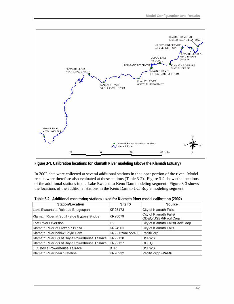
Model Configuration and Results
Figure 3-1. Calibration locations for Klamath River modeling (above the Klamath Estuary) In 2002 data were collected at several additional stations in the upper portion of the river. Model results were therefore also evaluated at these stations (Table 3-2). Figure 3-2 shows the locations of the additional stations in the Lake Ewauna to Keno Dam modeling segment. Figure 3-3 shows the locations of the additional stations in the Keno Dam to J.C. Boyle modeling segment. Table 3-2. Additional monitoring stations used for Klamath River model calibration (2002)
Station/Location Site ID Source
Lake Ewauna at Railroad Bridgespan KR25173 City of Klamath Falls
Klamath River at South-Side Bypass Bridge KR25079 City of Klamath Falls/ ODEQ/USBR/PacifiCorp
Lost River Diversion LK City of Klamath Falls/PacifiCorp
Klamath River at HWY 97 BR NE KR24901 City of Klamath Falls
Klamath River below Boyle Dam KR22129/KR22460 PacifiCorp
Klamath River u/s of Boyle Powerhouse Tailrace KR22128 USFWS
Klamath River d/s of Boyle Powerhouse Tailrace KR22127 ODEQ
J.C. Boyle Powerhouse Tailrace BTR USFWS
Klamath River near Stateline KR20932 PacifiCorp/SWAMP
42
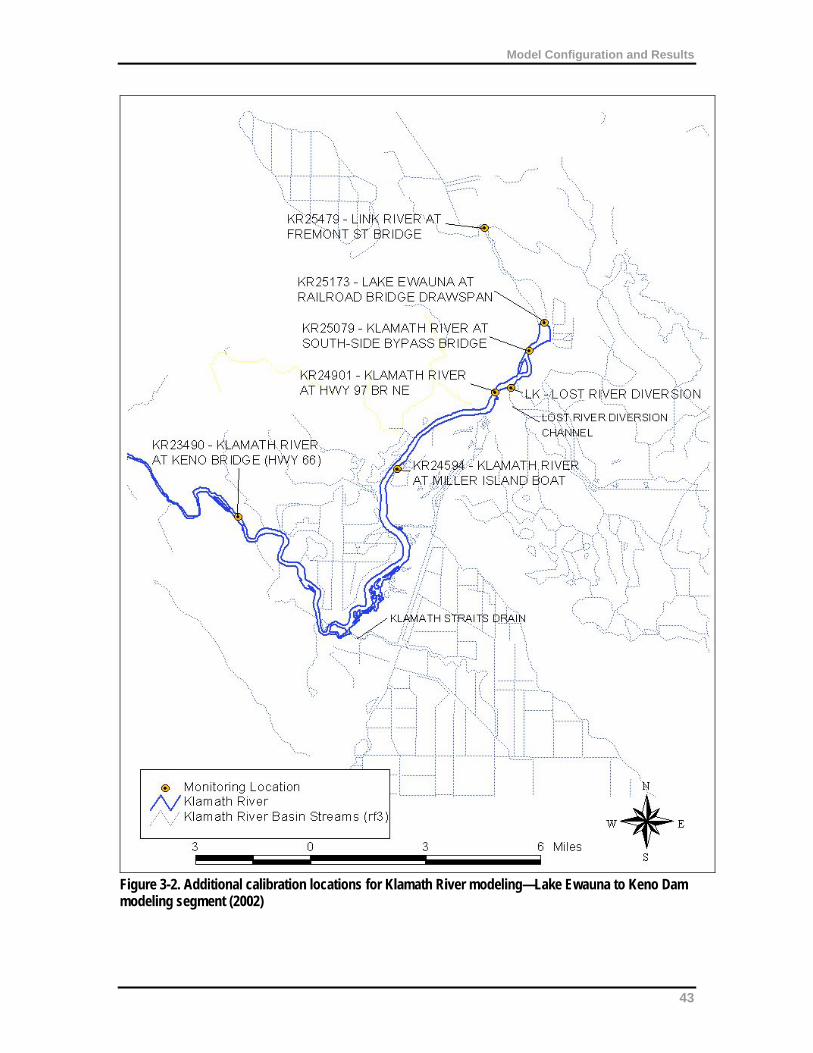
Model Configuration and Results
Figure 3-2. Additional calibration locations for Klamath River modeling—Lake Ewauna to Keno Dam modeling segment (2002)
43
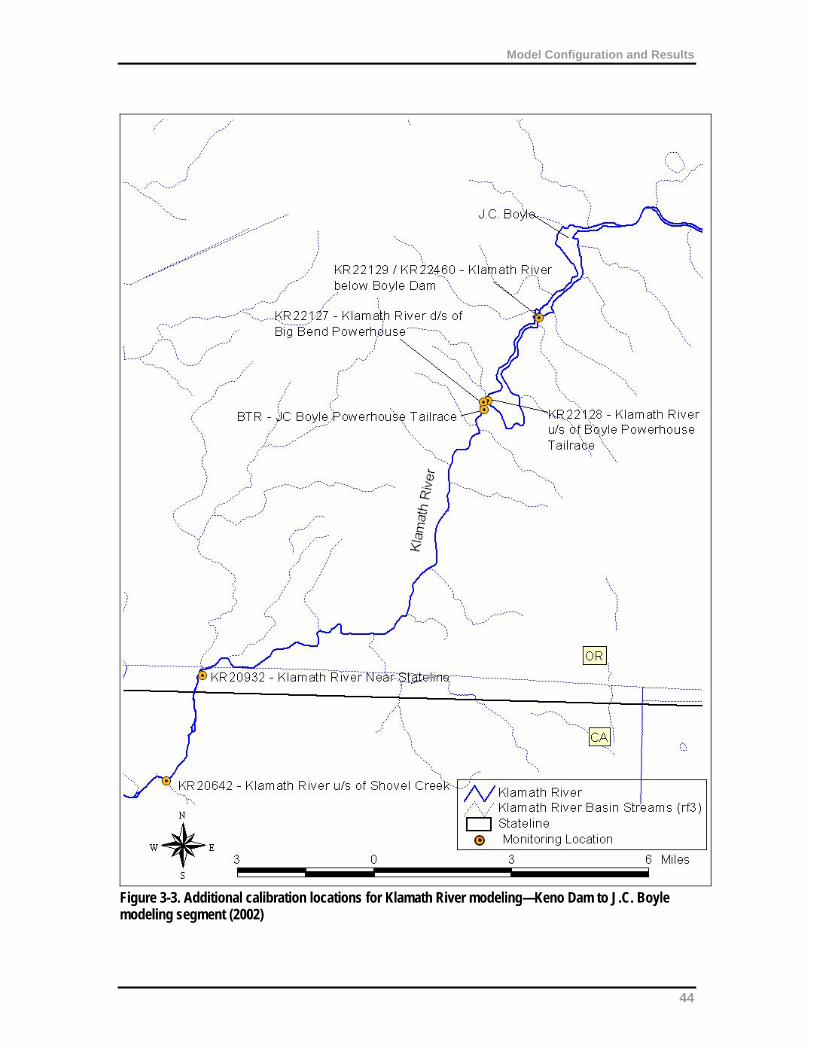
Model Configuration and Results
Figure 3-3. Additional calibration locations for Klamath River modeling—Keno Dam to J.C. Boyle modeling segment (2002)
44
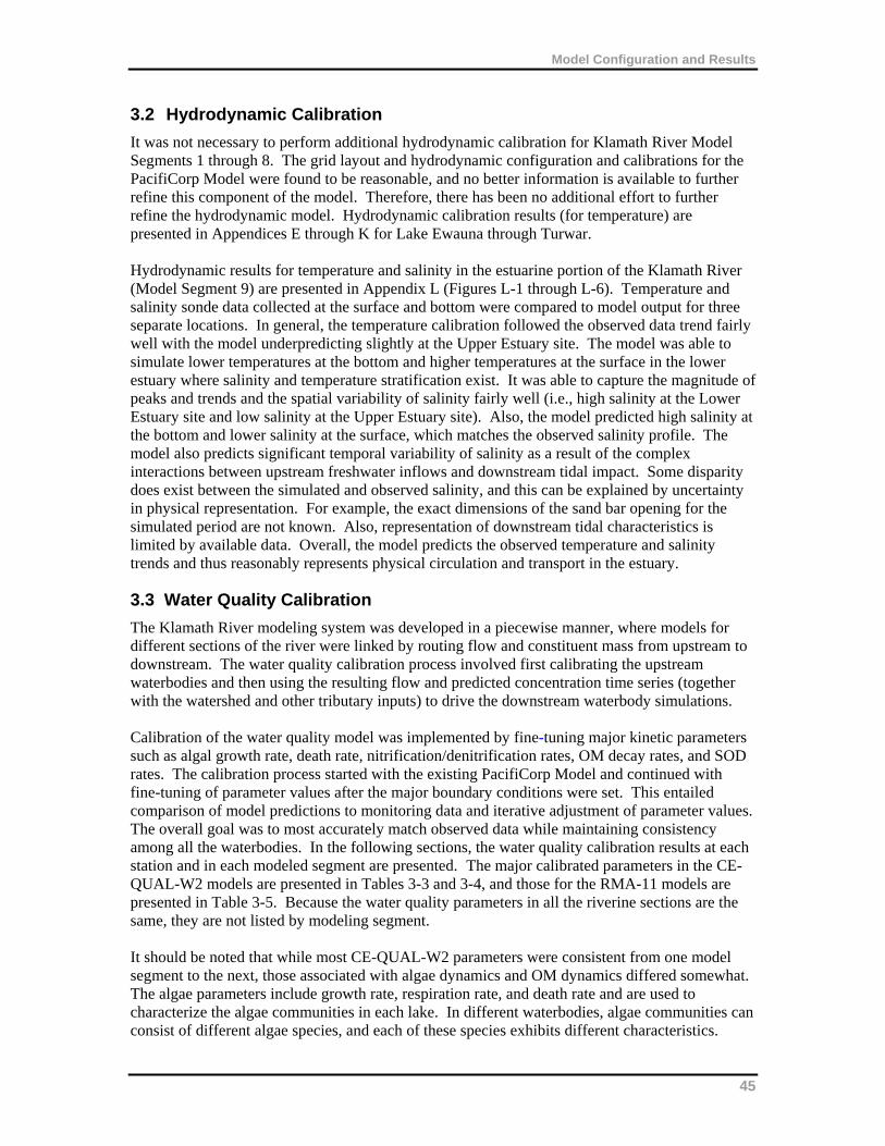
Model Configuration and Results
3.2 Hydrodynamic Calibration
It was not necessary to perform additional hydrodynamic calibration for Klamath River Model Segments 1 through 8. The grid layout and hydrodynamic configuration and calibrations for the PacifiCorp Model were found to be reasonable, and no better information is available to further refine this component of the model. Therefore, there has been no additional effort to further refine the hydrodynamic model. Hydrodynamic calibration results (for temperature) are presented in Appendices E through K for Lake Ewauna through Turwar. Hydrodynamic results for temperature and salinity in the estuarine portion of the Klamath River (Model Segment 9) are presented in Appendix L (Figures L-1 through L-6). Temperature and salinity sonde data collected at the surface and bottom were compared to model output for three separate locations. In general, the temperature calibration followed the observed data trend fairly well with the model underpredicting slightly at the Upper Estuary site. The model was able to simulate lower temperatures at the bottom and higher temperatures at the surface in the lower estuary where salinity and temperature stratification exist. It was able to capture the magnitude of peaks and trends and the spatial variability of salinity fairly well (i.e., high salinity at the Lower Estuary site and low salinity at the Upper Estuary site). Also, the model predicted high salinity at the bottom and lower salinity at the surface, which matches the observed salinity profile. The model also predicts significant temporal variability of salinity as a result of the complex interactions between upstream freshwater inflows and downstream tidal impact. Some disparity does exist between the simulated and observed salinity, and this can be explained by uncertainty in physical representation. For example, the exact dimensions of the sand bar opening for the simulated period are not known. Also, representation of downstream tidal characteristics is limited by available data. Overall, the model predicts the observed temperature and salinity trends and thus reasonably represents physical circulation and transport in the estuary.
3.3 Water Quality Calibration
The Klamath River modeling system was developed in a piecewise manner, where models for different sections of the river were linked by routing flow and constituent mass from upstream to downstream. The water quality calibration process involved first calibrating the upstream waterbodies and then using the resulting flow and predicted concentration time series (together with the watershed and other tributary inputs) to drive the downstream waterbody simulations. Calibration of the water quality model was implemented by fine-tuning major kinetic parameters such as algal growth rate, death rate, nitrification/denitrification rates, OM decay rates, and SOD rates. The calibration process started with the existing PacifiCorp Model and continued with fine-tuning of parameter values after the major boundary conditions were set. This entailed comparison of model predictions to monitoring data and iterative adjustment of parameter values. The overall goal was to most accurately match observed data while maintaining consistency among all the waterbodies. In the following sections, the water quality calibration results at each station and in each modeled segment are presented. The major calibrated parameters in the CE-QUAL-W2 models are presented in Tables 3-3 and 3-4, and those for the RMA-11 models are presented in Table 3-5. Because the water quality parameters in all the riverine sections are the same, they are not listed by modeling segment. It should be noted that while most CE-QUAL-W2 parameters were consistent from one model segment to the next, those associated with algae dynamics and OM dynamics differed somewhat. The algae parameters include growth rate, respiration rate, and death rate and are used to characterize the algae communities in each lake. In different waterbodies, algae communities can consist of different algae species, and each of these species exhibits different characteristics.
45
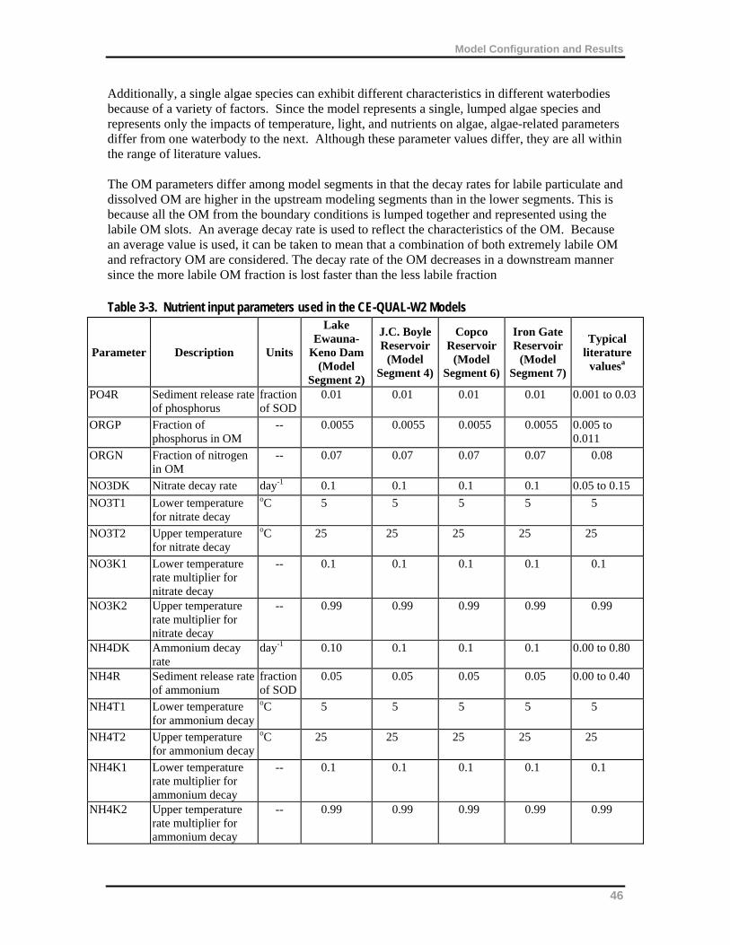
Model Configuration and Results
Additionally, a single algae species can exhibit different characteristics in different waterbodies because of a variety of factors. Since the model represents a single, lumped algae species and represents only the impacts of temperature, light, and nutrients on algae, algae-related parameters differ from one waterbody to the next. Although these parameter values differ, they are all within the range of literature values. The OM parameters differ among model segments in that the decay rates for labile particulate and dissolved OM are higher in the upstream modeling segments than in the lower segments. This is because all the OM from the boundary conditions is lumped together and represented using the labile OM slots. An average decay rate is used to reflect the characteristics of the OM. Because an average value is used, it can be taken to mean that a combination of both extremely labile OM and refractory OM are considered. The decay rate of the OM decreases in a downstream manner since the more labile OM fraction is lost faster than the less labile fraction Table 3-3. Nutrient input parameters used in the CE-QUAL-W2 Models
Parameter Description Units
Lake Ewauna-
Keno Dam (Model
Segment 2)
J.C. Boyle Reservoir
(Model Segment 4)
Copco Reservoir
(Model Segment 6)
Iron Gate Reservoir
(Model Segment 7)
Typical literature
valuesa
PO4R Sediment release rate of phosphorus
fraction of SOD
0.01 0.01 0.01 0.01 0.001 to 0.03
ORGP Fraction of phosphorus in OM
-- 0.0055 0.0055 0.0055 0.0055 0.005 to 0.011
ORGN Fraction of nitrogen in OM
-- 0.07 0.07 0.07 0.07 0.08
NO3DK Nitrate decay rate day-1 0.1 0.1 0.1 0.1 0.05 to 0.15
NO3T1 Lower temperature for nitrate decay
oC 5 5 5 5 5
NO3T2 Upper temperature for nitrate decay
oC 25 25 25 25 25
NO3K1 Lower temperature rate multiplier for nitrate decay
-- 0.1 0.1 0.1 0.1 0.1
NO3K2 Upper temperature rate multiplier for nitrate decay
-- 0.99 0.99 0.99 0.99 0.99
NH4DK Ammonium decay rate
day-1 0.10 0.1 0.1 0.1 0.00 to 0.80
NH4R Sediment release rate of ammonium
fraction of SOD
0.05 0.05 0.05 0.05 0.00 to 0.40
NH4T1 Lower temperature for ammonium decay
oC 5 5 5 5 5
NH4T2 Upper temperature for ammonium decay
oC 25 25 25 25 25
NH4K1 Lower temperature rate multiplier for ammonium decay
-- 0.1 0.1 0.1 0.1 0.1
NH4K2 Upper temperature rate multiplier for ammonium decay
-- 0.99 0.99 0.99 0.99 0.99
46
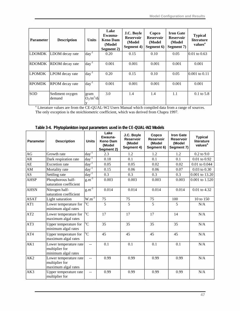
Model Configuration and Results
47
Parameter Description Units
Lake Ewauna-
Keno Dam (Model
Segment 2)
J.C. Boyle Reservoir
(Model Segment 4)
Copco Reservoir
(Model Segment 6)
Iron Gate Reservoir
(Model Segment 7)
Typical literature
valuesa
LDOMDK LDOM decay rate day-1 0.20 0.15 0.10 0.05 0.01 to 0.63
RDOMDK RDOM decay rate day-1 0.001 0.001 0.001 0.001 0.001
LPOMDK LPOM decay rate day-1 0.20 0.15 0.10 0.05 0.001 to 0.11
RPOMDK RPOM decay rate day-1 0.001 0.001 0.001 0.001 0.001
SOD Sediment oxygen demand
gram O2/m
2/day
3.0 1.4 1.4 1.1 0.1 to 5.8
a Literature values are from the CE-QUAL-W2 Users Manual which compiled data from a range of sources. The only exception is the stoichiometric coefficient, which was derived from Chapra 1997.
Table 3-4. Phytoplankton input parameters used in the CE-QUAL-W2 Models
Parameter Description Units
Lake Ewauna-
Keno Dam (Model
Segment 2)
J.C. Boyle Reservoir
(Model Segment 4)
Copco Reservoir
(Model Segment 6)
Iron Gate Reservoir
(Model Segment 7)
Typical literature valuesa
AG Growth rate day-1 2.3 1.2 1.2 1.2 0.2 to 9.0 AR Dark respiration rate day-1 0.18 0.1 0.1 0.1 0.01 to 0.92 AE Excretion rate day-1 0.05 0.05 0.02 0.02 0.01 to 0.044AM Mortality rate day-1 0.15 0.06 0.06 0.07 0.03 to 0.30 AS Settling rate day-1 0.3 0.3 0.3 0.3 0.001 to 13.20AHSP Phosphorous half-
saturation coefficient g.m-3 0.003 0.003 0.003 0.003 0.001 to 1.520
AHSN Nitrogen half-saturation coefficient
g.m-3 0.014 0.014 0.014 0.014 0.01 to 4.32
ASAT Light saturation W.m-3 75 75 75 100 10 to 150 AT1 Lower temperature for
minimum algal rates
oC 5 5 5 5 N/A
AT2 Lower temperature for maximum algal rates
oC 17 17 17 14 N/A
AT3 Upper temperature for minimum algal rates
oC 35 35 35 35 N/A
AT4 Upper temperature for maximum algal rates
oC 45 45 45 45 N/A
AK1 Lower temperature rate multiplier for minimum algal rates
-- 0.1 0.1 0.1 0.1 N/A
AK2 Lower temperature rate multiplier for maximum algal rates
-- 0.99 0.99 0.99 0.99 N/A
AK3 Upper temperature rate multiplier for
-- 0.99 0.99 0.99 0.99 N/A
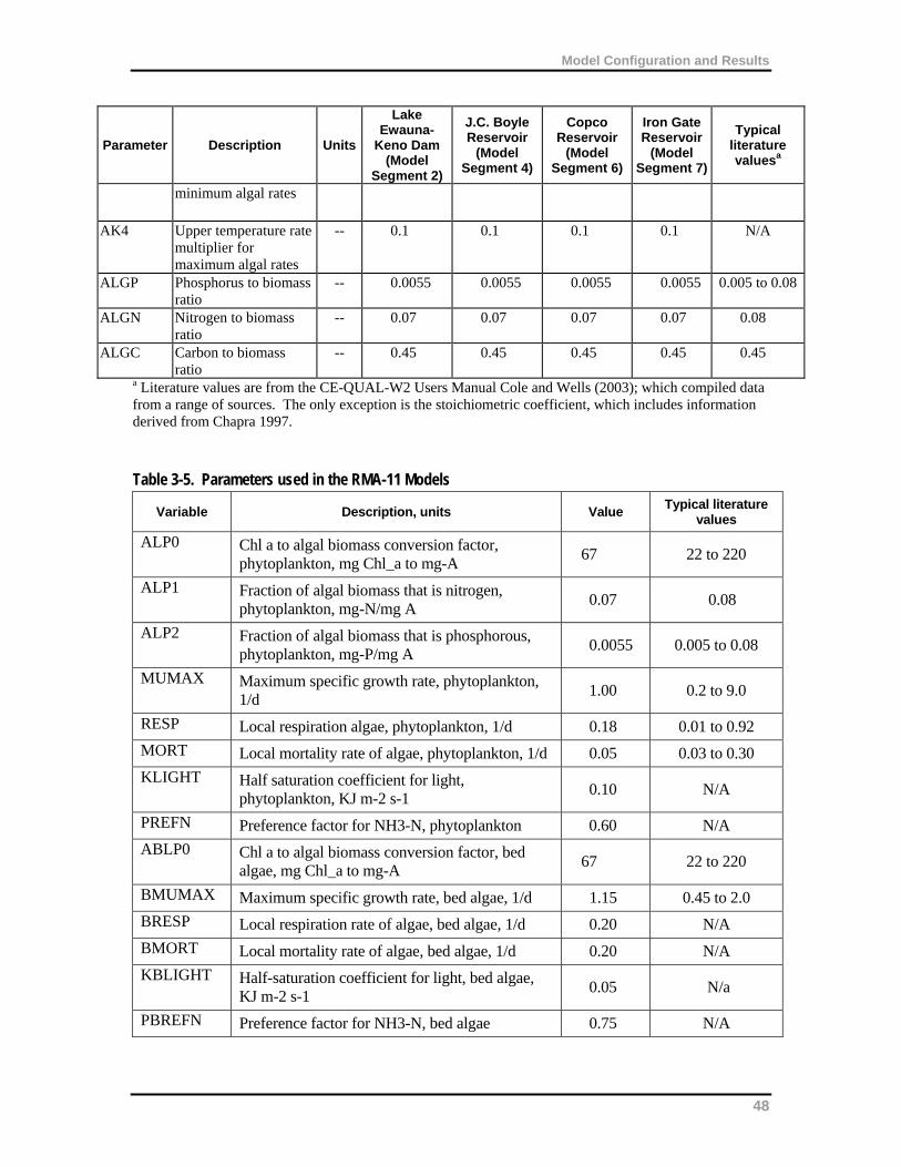
Model Configuration and Results
48
Parameter Description Units
Lake Ewauna-
Keno Dam (Model
Segment 2)
J.C. Boyle Reservoir
(Model Segment 4)
Copco Reservoir
(Model Segment 6)
Iron Gate Reservoir
(Model Segment 7)
Typical literature valuesa
minimum algal rates
AK4 Upper temperature rate multiplier for maximum algal rates
-- 0.1 0.1 0.1 0.1 N/A
ALGP Phosphorus to biomass ratio
-- 0.0055 0.0055 0.0055 0.0055 0.005 to 0.08
ALGN Nitrogen to biomass ratio
-- 0.07 0.07 0.07 0.07 0.08
ALGC Carbon to biomass ratio
-- 0.45 0.45 0.45 0.45 0.45
a Literature values are from the CE-QUAL-W2 Users Manual Cole and Wells (2003); which compiled data from a range of sources. The only exception is the stoichiometric coefficient, which includes information derived from Chapra 1997.
Table 3-5. Parameters used in the RMA-11 Models
Variable Description, units Value Typical literature
values
ALP0 Chl a to algal biomass conversion factor, phytoplankton, mg Chl_a to mg-A
67 22 to 220
ALP1 Fraction of algal biomass that is nitrogen, phytoplankton, mg-N/mg A
0.07 0.08
ALP2 Fraction of algal biomass that is phosphorous, phytoplankton, mg-P/mg A
0.0055 0.005 to 0.08
MUMAX Maximum specific growth rate, phytoplankton, 1/d
1.00 0.2 to 9.0
RESP Local respiration algae, phytoplankton, 1/d 0.18 0.01 to 0.92
MORT Local mortality rate of algae, phytoplankton, 1/d 0.05 0.03 to 0.30
KLIGHT Half saturation coefficient for light, phytoplankton, KJ m-2 s-1
0.10 N/A
PREFN Preference factor for NH3-N, phytoplankton 0.60 N/A
ABLP0 Chl a to algal biomass conversion factor, bed algae, mg Chl_a to mg-A
67 22 to 220
BMUMAX Maximum specific growth rate, bed algae, 1/d 1.15 0.45 to 2.0
BRESP Local respiration rate of algae, bed algae, 1/d 0.20 N/A
BMORT Local mortality rate of algae, bed algae, 1/d 0.20 N/A
KBLIGHT Half-saturation coefficient for light, bed algae, KJ m-2 s-1
0.05 N/a
PBREFN Preference factor for NH3-N, bed algae 0.75 N/A
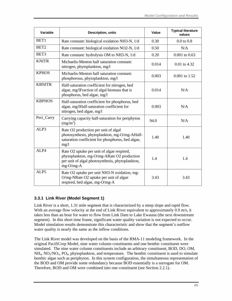
Model Configuration and Results
49
Variable Description, units Value Typical literature
values
BET1 Rate constant: biological oxidation NH3-N, 1/d 0.30 0.0 to 0.8
BET2 Rate constant: biological oxidation NO2-N, 1/d 0.50 N/A
BET3 Rate constant: hydrolysis OM to NH3-N, 1/d 0.20 0.001 to 0.63
KNITR Michaelis-Menton half saturation constant: nitrogen, phytoplankton, mg/l
0.014 0.01 to 4.32
KPHOS Michaelis-Menton half saturation constant: phosphorous, phytoplankton, mg/l
0.003 0.001 to 1.52
KBNITR Half-saturation coefficient for nitrogen, bed algae, mg/lFraction of algal biomass that is phosphorus, bed algae, mg/l
0.014 N/A
KBPHOS Half-saturation coefficient for phosphorus, bed algae, mg/lHalf-saturation coefficient for nitrogen, bed algae, mg/l
0.003 N/A
Peri_Carry Carrying capacity half-saturation for periphyton (mg/m2)
94.0 N/A
ALP3 Rate O2 production per unit of algal photosynthesis, phytoplankton, mg-O/mg-AHalf-saturation coefficient for phosphorus, bed algae, mg/l
1.40 1.40
ALP4 Rate O2 uptake per unit of algae respired, phytoplankton, mg-O/mg-ARate O2 production per unit of algal photosynthesis, phytoplankton, mg-O/mg-A
1.4 1.4
ALP5 Rate O2 uptake per unit NH3-N oxidation, mg-O/mg-NRate O2 uptake per unit of algae respired, bed algae, mg-O/mg-A
3.43 3.43
3.3.1 Link River (Model Segment 1)
Link River is a short, 1.31 mile segment that is characterized by a steep slope and rapid flow. With an average flow velocity at the end of Link River equivalent to approximately 0.9 m/s, it takes less than an hour for water to flow from Link Dam to Lake Ewauna (the next downstream segment). In this short time frame, significant water quality variation is not expected to occur. Model simulation results demonstrate this characteristic and show that the segment’s outflow water quality is nearly the same as the inflow conditions. The Link River model was developed on the basis of the RMA-11 modeling framework. In the original PacifiCorp Model, nine water column constituents and one benthic constituent were simulated. The nine water column constituents include an arbitrary constituent, BOD, DO, OM, NH4, NO2/NO3, PO4, phytoplankton, and temperature. The benthic constituent is used to simulate benthic algae such as periphyton. In this system configuration, the simultaneous representation of the BOD and OM provide some redundancy because BOD essentially is a surrogate for OM. Therefore, BOD and OM were combined into one constituent (see Section 2.2.1).
Model Configuration and Results
The model was run for the period from January 1, 2000, to December 31, 2000 for the 2000 calibration run. I It was also run from January 1, 2002 to December 31, 2002 for the corroboration run. No data were available to calibrate the model for the reach.
3.3.2 Lake Ewauna-Keno Dam (Model Segment 2)
The Lake Ewauna segment was developed on the basis of the CE-QUAL-W2 modeling framework. In the original PacifiCorp Model, 18 water column constituents were simulated, which included four OM components and one BOD component. In the present study, BOD was eliminated from the active constituent list in the model input data file (see Section 2.2.1). In the calibration run, the model was run for the period from January 1, 2000, to December 31, 2000. The model output was compared to observations at two water quality stations in Lake Ewauna: Klamath River at Miller Island boat ramp and Klamath River at Keno bridge (Hwy 66). As shown in Figures E-1 through E-16 in Appendix E, the model reproduced the observed water quality pattern reasonably well. The final calibrated parameters for Lake Ewauna are presented in Tables 3-3 and 3-4. The model reproduces the supersaturation of DO in June well, as well as the extended anoxic period in July. The DO data show strong diurnal fluctuation and supersaturation conditions during May, however, it seems to contradict the phytoplankton data. Phytoplankton data exhibit low chlorophyll a concentrations during this period, and these concentrations are insufficient to generate the supersaturated DO concentrations observed in the water column. Since the May chlorophyll a data correspond with algae levels in UKL, it was assumed that the DO concentrations in May are not entirely reliable. Therefore, no attempt was made to reproduce the supersaturation in May. The model also was able to reproduce DO recovery in early August and the subsequent dip in late August and through September. It is worth noting that the data show low DO in late fall and winter while the model simulates relatively high DO concentrations. During this period, water temperature dropped rapidly, and algae and OM loading from UKL decreased. One would expect that these monitored phenomena would result in DO recovery from the summer anoxic conditions (as predicted by the model). Lake Ewauna, however, is a unique system that is highly dynamic and subject to tremendous OM loading from UKL. The lake also experiences an extended period of summer hypoxic/anoxic conditions which result in quick removal of algae and generation of extra OM. Therefore, it is highly likely that the lake’s late fall and winter DO concentrations do not respond similarly to most other impoundments. One possible cause might be that the extremely high organic loading from both UKL and algae death during the summer result in a tremendous amount of OM being settled into the sediment layer during the summer (forming a highly enriched bed). During late fall and winter, even though OM and algae loadings cease, this highly enriched bed may provide significant oxygen consumption potential (preventing high DO concentrations). This could be the ultimate cause of the observed low DO during the late fall and winter. Without a predictive sediment diagenesis module, however, the existing CE-QUAL-W2 model is not capable of fully representing the dynamic interaction and feedback between the sediment and water column. This limitation is not expected to impact TMDL determination, because the critical, anoxic period occurs during the summer. The predicted phytoplankton biomass matches the observed trends very well, especially the decline during the summer anoxic period and the difference in magnitude between Miller Island
50
Model Configuration and Results
and Hwy 66. The model does overpredict chlorophyll a during the month of June at both Miller Island and Hwy 66 due to the lack of temporally variable data in UKL to set the boundary condition. The boundary condition data for UKL shows a chlorophyll a peak during June, and this is transported quickly downstream, resulting in the peak in June at Miller Island and Hwy 66. In general, the model also predicts nutrients well, except for timing in some situations. This is likely because of limitations surrounding the definition of boundary conditions (i.e., the use of limited data to derive the boundaries). The model was able to predict relatively high NH4 and PO4 concentrations during the anoxic period likely due to a combination of multiple water quality processes including upstream and tributary loading, OM decay, algae die-off, and release from sediment. It should be noted that simulated NO2/NO3 is relatively low compared with the observed values. The accuracy of these data, however, is unknown. Measurements made by different agencies during this time period were found to be significantly different (approximately an order of magnitude). It is suspected that the high NO2/NO3 measurements are incorrect. During the summer anoxic period, nitrification, which is the source of NO2/NO3, is inhibited by the low DO concentration. NO2/NO3 levels are expected to be high only if an external source is supplying a significant amount. This, however, is not supported by currently available data. The model predicts the trends exhibited by the lower level NO2/NO3 measurements. The model results also show good agreement between the simulated and observed pH at the two locations, indicating a reasonable representation of the fate and transport of pH related constituents and their interactions. The Lake Ewauna to Keno Dam model segment was further tested using monitoring data in 2002. In 2002 the city of Klamath Falls collected a significant amount of data in this reach. Data were collected at six monitoring stations, including Lake Ewauna at Railroad Bridge Drawspan (LERBD), Klamath River at South Side Bypass Bridge (KRSSBB), Klamath River at Hwy 97 (KR97), Klamath River at Lost River Diversion Channel (KRLRDC), Klamath River at Miller Island (KRMI), and Klamath River at Hwy 66 (KR66). The simulated temperature, nutrients, DO, and algae biomass are plotted against the observed data at these locations in Figures E-17 to E-57. The model reproduces the observed water quality conditions and trends well. A disparity between observed and modeled DO does exist between March and June. During this period, the model tends to underpredict DO. This suggests that the estimated OM boundary condition at Link River might be too high for this period and results in excessive deoxygenation potential in the water column. More representative monitoring data characterizing this boundary would improve the model predictions. Fortunately this time period is outside the critical summer months of July and August. Another observation is that the model tends to overpredict chlorophyll a during the month of June. This might be due to uncertainty in the upstream boundary condition as well as possible inter-year variability in water column kinetic characteristics that cannot be accounted for by using the same parameter values as in the 2000 calibration model. Despite this minor disparity between model results and data, the 2002 model represents the chlorophyll a trends well. Model results from 2000 can also be used to determine the significance of nutrient limiting effects on algae growth. Figure E-62 presents the simulated nutrient limiting condition at Hwy66 in 2000. Due to the high incoming nutrient loading from UKL, as well as significant contributions from LRDC and KSD, nutrient limiting factors for both nitrogen and phosphorus are very high (>0.9). This indicates that algae growth is not limited by nutrient availability. If either nutrient group (i.e., phosphorus or nitrogen) showed a significant divergence from a value of 1.0, nutrient availability would be limiting algae growth. In the spring, it appears that nitrogen might be slightly more limiting than phosphorus.
51
Model Configuration and Results
3.3.3 Keno Dam to J.C. Boyle Reservoir (Model Segment 3)
The portion of the water quality model for Keno Reach was developed using the RMA-11 modeling framework. In the original PacifiCorp Model, nine water column constituents and one benthic constituent were simulated as in the Link River model. In this river segment, BOD and OM were combined to form a unified constituent as was done for the Link River model segment. The model was run for the period from January 1, 2000, to December 31, 2000. No data were available to calibrate the model for the year 2000. Data were available for the year 2002 at a location downstream of Keno Dam. Figures F-1 through F-7 in Appendix F show the calibration results for the year 2002. The model reproduces the observed nutrients and pH well. The model results for DO also match the observed magnitudes and trends well. It does, however, predict a lower DO than the data show during the summer (Figure F-2). One reason might be that the model is not representing sufficient reaeration downstream of the dam. This would result in slower recovery from the low DO conditions seen upstream of the dam. It should also be noted that only one monitoring point is available during this extended time period. A single DO sample is insufficient to reflect the likely range of DO levels that would occur over a day and throughout this critical time period.
3.3.4 J.C. Boyle Reservoir (Model Segment 4)
The J.C. Boyle Reservoir segment was developed using the CE-QUAL-W2 modeling framework. The model was run for the period from January 1, 2000, to December 21, 2000. The constituent configuration in this river segment is the same as the Lake Ewauna segment (Section 3.3.2). For calibration, the model was run for the period from January 1, 2000, to December 31, 2000, and the simulated water quality is compared with observed profiles in the reservoir at water quality monitoring station J.C. Boyle Reservoir (at deepest point). Major parameters adjusted during the calibration process included algae growth rate, algae respiration rate, algae death rate, particulate OM settling velocity, OM decay rate, and suspended solids settling velocity. As shown in Figures G-1 through G-7 in Appendix G, the model reproduced the observed pattern reasonably well. Although the model overpredicts NH4 and NO3 concentrations on some dates and underpredicts them on other dates, it predicts concentrations within the range of observed data. These differences are caused by uncertainty in boundary conditions. To more accurately represent such fine-scale variability (both temporally and on a depth basis), higher resolution data (i.e., temporally and spatially) are necessary to configure boundary conditions representing major tributaries and inflows. The final calibrated parameters for J.C. Boyle Reservoir are presented in Tables 3-3 and 3-4. The J.C. Boyle model was further tested using the 2002 data. Only three constituents are available for 2002: temperature, pH, and DO. Model predictions for these constituents follow the overall trends well and suggest a reasonable calibration (Figures G-8 through G-10 in Appendix G).
52
Model Configuration and Results
3.3.5 Bypass/Full Flow Reach (Model Segment 5)
The Bypass/Full Flow Reach segment was developed using the RMA-11 modeling framework. In the original PacifiCorp Model, nine water column constituents and one benthic constituent were simulated as in the Link River model. In this study, BOD and OM are combined to form a unified constituent as was done for Link River model (see Section 2.2.1). For calibration, the model was run for the period from January 1, 2000, to December 31, 2000. Data for temperature, nutrients, DO, Alkalinity, and pH were available to calibrate the model. Figures H-26 through H-33 in Appendix H show the comparison of model results versus observed data for the Klamath River upstream of Shovel Creek. The results indicate reasonable agreement between predictions and monitoring data. The overprediction of chlorophyll a during June is due to uncertainty in the UKL boundary condition. Similarly, the overprediction of NH4 during summer and fall can also be attributed to uncertainty in the upstream boundary conditions in Lake Ewauna. The model was further tested using data collected in 2002 and was run from January 1, 2002, through December 31, 2002. Figures H-34 through H-40 in Appendix H show the comparison of model results versus observed data for the Klamath River upstream of Shovel Creek. In 2002 data were collected at more locations, including at the Klamath River downstream of J.C. Boyle Dam (KRJCB) (but upstream of the J.C. Boyle Powerhouse), Klamath River upstream of J.C. Boyle Powerhouse Tailrace (KRUPT), Klamath River downstream of Big Bend Powerhouse (KRBP), Klamath River at J.C. Boyle Powerhouse Tailrace (KRPT), and Klamath River near Stateline (KRS). The sampled constituents include temperature, DO, pH, and nutrients. The predicted results are plotted against the data in Appendix H (Figures H-1 to H-25). As shown, the model accurately reproduces the general trends and magnitudes observed in the data. There are, however, some discrepancies between model results and data at various locations and times. For example, Figure H-1 shows that although the model has reproduced the seasonal variability and peaks of temperature downstream of J.C. Boyle, it underpredicts the diurnal fluctuation. This discrepancy may be due to local conditions not entirely captured by the model. Data collection could have occurred in a shallow region that exhibits a wider range of temperature variability while the model segment represents laterally and vertically averaged. This particular location is almost immediately downstream of J.C. Boyle, and thus a significant amount of water is always discharged from the dam (greater than 100 cfs). Under these conditions, the average temperature in this segment should be primarily controlled by the discharge temperature from the dam. The model reflects this condition while the data could actually represent a highly localized condition. The discrepancy between model results and DO data in Figure H-2 is likely also caused by this same condition. Figures H-7 and H-10 show that the model slightly overpredicts and underpredicts, respectively, the observed temperatures. This is likely due to differences between the modeled spring water flow and temperature and actual conditions in these portions of the river data. For example, the model represents the spring discharge in this area as three discrete tributaries with constant flow rates and temperatures. In reality, the spring discharge can be variable in quantity as well as temperature. The model’s overprediction of chlorophyll a in Figure H-17 is likely caused by the overprediction of chlorophyll a in Lake Ewauna during the early summer, which propagate to this location in the system. Neither nitrogen nor phosphorus appears to significantly limit algae growth in this portion of the river. Figure H-41 presents the simulated nutrient limiting factors on periphyton growth for both nutrient classes during 2000, at Stateline. Neither nutrient class diverges significantly from a
53
Model Configuration and Results
value of 1.0. As with the Hwy66 location, nitrogen appears to be slightly more limiting than phosphorus in the spring.
3.3.6 Copco Reservoir (Model Segment 6)
The water quality model for Copco Reservoir was developed on the basis of the CE-QUAL-W2 modeling framework. The water quality constituent configuration in this segment is the same as for the Lake Ewauna segment. The model was run for the period from January 1, 2000, to December 31, 2000. The simulated water quality output was compared with the observed profile data in the reservoir at water quality station Copco Lake near Copco. Key parameters that were changed through this calibration process include algae growth rate (AG), particulate organic matter settling velocity (POMS), labile dissolved organic matter decay rate (LDOMDK), and labile particulate organic matter decay rate (LPOMDK). The final calibrated parameters for Copco Reservoir are presented in Tables 3-3 and 3-4. The model results are plotted against observed data at water quality station Copco Lake near Copco in Figures I-1 through I-7 in Appendix I. The model matched the monitoring data reasonably well. It overpredicts NH4 and NO3 concentrations on some dates and underpredicts them on other dates for Copco Reservoir. In general, however, it predicts concentrations within the range of observed data. Differences are likely caused by uncertainty in boundary conditions from limited data availability.
3.3.7 Iron Gate Reservoir (Model Segment 7)
The model was run for the period from January 1, 2000, to December 21, 2000. The simulated water quality output was compared with the observed profile data in the reservoir at the water quality station in Iron Gate Reservoir (Figures J-1 through J-7 in Appendix J). The Iron Gate Reservoir portion of the model was updated using the new parameter values from Copco Reservoir. It was found that by changing the values of several kinetic parameters, including SOD, AG, LDOMDK, and LPOMDK (as shown in Table 3-3 and 3-4), the model was able to predict a reasonable water quality response for DO, phytoplankton, and nutrients. Additional parameters that were fine-tuned include sediment NH4 release rate in proportion to SOD (NH4R), sediment PO4 release rate in proportion to SOD (PO4R), algae death rate (AM). The detailed parameter values are listed in Tables 3-3 and 3-4. The model achieves a reasonable agreement with the data, indicating that the water quality dynamics in the reservoir are reasonably represented.
3.3.8 Iron Gate Dam to Turwar (Model Segment 8)
The water quality model for this segment was developed using the RMA-11 modeling framework, and the water quality constituent configuration is the same as for the upstream riverine RMA models. The model was run for the period from January 1, 2000, to December 31, 2000. Data for only temperature and DO were available at five stations along this reach to calibrate the model. The five stations are the Klamath River downstream of Iron Gate Dam, Klamath River above Shasta
54
Model Configuration and Results
River, Klamath River above Scott River, Klamath River above Seiad Valley, and Klamath River at Youngs Bar. Model results are plotted against observed data in Appendix K. The model reproduces the observed temperature very well at these locations. The model also reproduces DO concentrations. As noted earlier in this report, a scaling factor was introduced into the RMA-11 model to better represent reaeration just downstream of Iron Gate Dam. The scaling factor was determined through an inverse modeling process which involved estimating reaeration based on upstream and downstream DO concentrations. DO predictions further downstream generally also replicate monitoring data. The Klamath River is steep and is generally characterized by a large flow. This results in significant reaeration along the length of the river. Modeling results for this segment show that DO in the river increases to approximately saturation because of this reaeration effect. At monitoring locations farther downstream, e.g., above Seiad Valley and at Youngs Bar, data however do not show this expected trend. In fact, the model tends to overpredict DO. Observed DO can reach very low levels, e.g., 2.5 to 4.0 mg/L; however, the model tends to predict concentrations around 8.0 mg/L (close to saturation).
This disparity in results was investigated through a number of sensitivity analyses. The following adjustments to the model were made to determine their potential effect on in-stream DO concentrations:
Tributary DO boundary conditions were reduced to 0.0 mg/L (for all incoming tributaries where monitoring data are available, except major rivers such as Shasta and Scott).
SOD was increased to an extremely high value along the length of the river (to 5.0 g/m2/day). This represents a highly enriched substrate, although this is uncharacteristic of this region of the Klamath River.
A very high OM concentration was set for all boundary conditions. The value used is equivalent to roughly 45.0 mg/L of CBOD.
A series of different reaeration equations were used. None of these adjustments was able to sufficiently lower the DO concentrations to the monitoring levels. It should also be noted that the low DO does not appear to be caused by biological activity (e.g., periphyton), based on the minimal observed diel DO fluctuation range. After running these sensitivity analyses, the quality of the DO monitoring data were further explored. Upon further review, DO data for this time period were found to be inaccurate. The Klamath River Water Quality 2000 Monitoring Program—Project Report (Watercourse Engineering, Inc. 2003) indicated that biofouling of the DO membrane was an issue at nearly all monitoring locations (including the locations identified in this section for model calibration). Biofouling refers to the impact of biological activity on instrumentation, and it results in inaccurate DO measurements. It typically occurred within 24 to 96 hours of probe deployment and resulted in degradation (i.e., reduction) of DO concentrations. The extent of degradation in measurements is apparent from the DO monitoring data plotted in Appendix K. Sudden step increases of 2 to 3 mg/L occur multiple times over the course of the summer (e.g., beginning of August and September at the Youngs Bar station). These increases occur when a probe is removed, cleaned, and re-deployed. Subsequent to these increases, the DO concentrations again decline. Because of these inaccuracies, the model predictions should not (and do not) closely match the measured DO levels. The model predictions do tend to follow the trend in maximum DO concentrations measured for this period (where biofouling is not an issue).
55
Model Configuration and Results
In this stretch of the river, nutrient limitation is a more significant factor than at upstream locations. Figure K-26 suggests that nitrogen becomes a factor that can limit periphyton growth at Turwar during the late spring and summer. The limiting factor value for nitrogen falls to 0.4 while that for phosphorus remains close to 1.0. This significant divergence from 1.0 for nitrogen is more pronounced at this location than at Hwy66 or Stateline.
3.3.9 Klamath Estuary - Turwar to the Pacific Ocean (Model Segment 9)
EFDC was used to model this portion of the Klamath River. The simulated water quality output was compared with grab sample data and measured DO sonde data at three water quality stations in the lower, middle, and upper estuary for the year 2004 (Figures L-7 through L-9 in Appendix L). Calibration data were available for 2004 because of an intensive monitoring effort conducted by the NCRWQCB and Yurok Tribe in June, July, August, and September. Data were collected as grab samples at the surface and bottom of the estuary for a suite of nutrients along with algae measurements and sonde data measurements for temperature, DO, and salinity. Continuous sonde data were collected each month for 4–5 days at the surface and bottom. The water quality constituents evaluated for calibration include chlorophyll a, DO (surface and bottom), PO4, NH4, and NO2/NO3 at each of the three locations in the estuary. Although the grab sampling data provided a variety of data for calibration, all except one data point for PO4, NH4 and NO2/NO3 were reported as non-detects. It was noted that these samples were diluted, and that the reporting limit was raised on the basis of different dilutions (e.g., 5x, 10x and 20x) for different sampling days (because of matrix interference, possibly chloride). To consider this uncertainty in the data, error bars were provided in the calibration figures in Appendix L. These bars show the potential range of the laboratory measurements. The lower bound was estimated as half of the lowest report limit. The water quality predictions follow the overall trends and magnitudes at the calibration locations fairly well. DO concentrations at the surface and bottom locations are replicated, and the model is able to predict low DO conditions during the summer period. The model also reproduces the observed diel fluctuation of DO in both the surface and bottom water. Since the model and observed data both show very low algae concentrations in the estuary, significant diel fluctuations of DO do not occur as a result of phytoplankton. Periphyton biomass, however, is predicted at high levels in the shallow regions of the estuary. This is likely a key contributor to diel DO fluctuation. Periphyton also influences diel fluctuation of nutrients. Table 3-6 presents the calibration parameter values for the EFDC model.
This space intentionally left blank
56
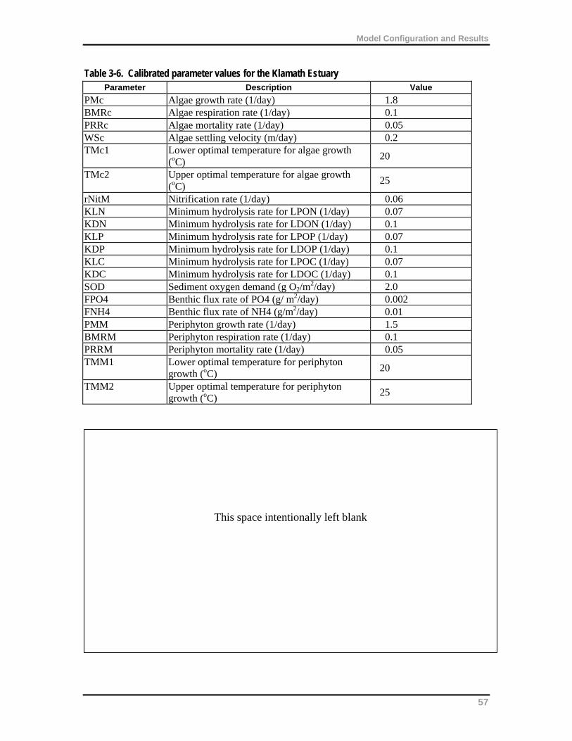
Model Configuration and Results
Table 3-6. Calibrated parameter values for the Klamath Estuary Parameter Description Value
PMc Algae growth rate (1/day) 1.8 BMRc Algae respiration rate (1/day) 0.1 PRRc Algae mortality rate (1/day) 0.05 WSc Algae settling velocity (m/day) 0.2 TMc1 Lower optimal temperature for algae growth
(oC) 20
TMc2 Upper optimal temperature for algae growth (oC)
25
rNitM Nitrification rate (1/day) 0.06 KLN Minimum hydrolysis rate for LPON (1/day) 0.07 KDN Minimum hydrolysis rate for LDON (1/day) 0.1 KLP Minimum hydrolysis rate for LPOP (1/day) 0.07 KDP Minimum hydrolysis rate for LDOP (1/day) 0.1 KLC Minimum hydrolysis rate for LPOC (1/day) 0.07 KDC Minimum hydrolysis rate for LDOC (1/day) 0.1 SOD Sediment oxygen demand (g O2/m
2/day) 2.0 FPO4 Benthic flux rate of PO4 (g/ m2/day) 0.002 FNH4 Benthic flux rate of NH4 (g/m2/day) 0.01 PMM Periphyton growth rate (1/day) 1.5 BMRM Periphyton respiration rate (1/day) 0.1 PRRM Periphyton mortality rate (1/day) 0.05 TMM1 Lower optimal temperature for periphyton
growth (oC) 20
TMM2 Upper optimal temperature for periphyton growth (oC)
25
This space intentionally left blank
57
Model Configuration and Results
REFERENCES Arhonditsis, G.B. and M.T. Brett. 2004. Evaluation of the current state of mechanistic aquatic
biogeochemical modeling. Marine Ecology Progress Series 271: 13-26. Baric, A., B. Grbec, G. Kuspilic, I. Marasovic, Z. Nincevic, and I. Grubelic. 2003. Mass
Mortality Event in a Small Saline Lake (Lake Rogoznica) caused by Unusual Holomictic Conditions. Scientia Marina 67(2):129–141.
Cole, T.M. and S.A. Wells. 2003. CE-QUAL-W2: A two-dimensional, laterally averaged,
Hydrodynamic and Water Quality Model, Version 3.1, Instruction Report EL-03-1, US Army Engineering and Research Development Center, Vicksburg, MS.
Chapra, S.C. 1997. Surface Water-Quality Modeling. McGraw-Hill, Inc., New York. Deas, M. 2000. Application of numerical water quality model in ecological assessment. Ph.D.
dissertation. University of California, Davis. Flint, L.E. and Flint, A.L., 2008. A Basin-Scale Approach to Estimating Stream Temperatures of
Tributaries to the Lower Klamath River, California. J Environ Qual 37:57-68. McGlashan, H.D. and H.J. Dean. 1913. Surface Water Supply of the United States 1913, Part XI,
Pacific Slope Basins in California. USGS Water Supply Paper 300. Washington: Government Printing Office.
National Research Council. 2004. Endangered and Threatened Fishes in the Klamath Basin.
Committee on Endangered and Threatened Fishes in the Klamath River Basin, The National Academies Press, Washington, DC.
NCRWQCB. 2008. Analysis of Klamath Tributary Data. North Coast Regional Water Quality
Control Board. July 2, 2008. PacifiCorp. 2005. Klamath River Water Quality Model Implementation, Calibration, and
Validation. Klamath Hydroelectric Project (FERC Project No. 2082) - Response to November 10, 2005, FERC AIR GN-2. December 16, 2005, FERC filing.
Park, K., A.Y. Kuo, J. Shen, and J.M. Hamrick. 1995. A three-dimensional hydrodynamic-
eutrophication model (HEM-3D): description of water quality and sediment process submodels. Special Report in Applied Marine Science and Ocean Engineering No. 327. School of Marine Science Virginia Institute of Marine Science, College of William and Mary, January 1995.
Tetra Tech, Inc. 2004. Data Review and Modeling Approach – Klamath and Lost Rivers TMDL
Development. Prepared for U.S. Environmental Protection Agency Region 10, U.S. Environmental Agency Region 9, Oregon Department of Environmental Quality, and North Coast Regional Water Quality Control Board.
58

Model Configuration and Results
59
Watercourse Engineering, Inc. 2003. Klamath River Water Quality 2000 Monitoring Program - Project Report. Prepared for U.S. Bureau of Reclamation with support from PacifiCorp. (January, 25, 2003).
Watercourse Engineering, Inc. 2004. Klamath River Modeling Framework to Support the
PacifiCorp Federal Energy Regulatory Commission Hydropower Relicensing Application [DRAFT] Prepared for PacifiCorp (March 9, 2004).