The Kinetics of the Saponification of Ethylacetate1,2

Purpose: Determine the order, rate constant, activation energy, and pre-exponential factor for the

reaction of ethylacetate with base using conductance measurements.

Prelab: Make sure to do all solution preparation calculations before you come to lab.

Introduction

This experiment studies the rate of the reaction of ethylacetate with base to give the acetate ion

and ethyl alcohol:

CH3COOCH2CH3 + OH- CH3COO

- + CH2CH3OH

This reaction is often called saponification. An application of saponification is the manufacture

of soaps. The base in this experiment is NaOH. For the purposes of this experiment, it can be

assumed that this reaction runs essentially to completion. The position of equilibrium lies far to

the right.

The proposed mechanism for the reaction starts with the nucleophilic attack of the hydroxide

ion on the carboxyl carbon to form a tetrahedral intermediate and the subsequent loss of the

alkoxide as the leaving group:

H3C

O

O

CH3

H3C

O

OH

O

CH3

H3C

OH

O

O

CH3

HO

+

These steps are followed by a fast H+ ion transfer to give the acetate ion:

H3C

OH

O

O

CH3

+ H3C

O

O

HO

CH3

+

Is this mechanism consistent with the observed rate law? In this experiment we will determine

the rate law and the temperature dependence of the rate constant. This reaction can be followed

using conductivity, because the molar conductivity of acetate ions is much smaller than the molar

conductivity of hydroxide ions. However, there will also be a large background conductivity

from the Na+ counter ions from the base. The conductivity of the Na

+ ions will be approximately

constant during the course of the reaction.

Kinetics 2

The Rate Expression

The rate expression for a chemical reaction can only be obtained from experimental data. From

the experimental rate expression, a detailed mechanism for the reaction can be developed. In

general, consider the rate of a general chemical reaction:

a A + b B c C + d D 1

The rates of appearance of the products or the disappearance of the reactants are related to the

overall reaction rate by:

rate = – 1

a d[A]

dt = –

1

b d[B]

dt =

1

c d[C]

dt =

1

d d[D]

dt 2

where the brackets refer to concentrations generally in mol L-1. The rate expression often has the

form

rate = k [A]n[B]m 3

where k is the rate constant and n and m are the reaction order with respect to each reactant. The

concentrations of products and catalysts can also occur in the rate law. There is no relationship

between the values of the reaction orders, n and m, and the stoichiometric coefficients, because

the reaction may occur in more than one mechanistic step.

Isolation Method

For complicated reactions it is often useful to simplify the rate law by setting the concentrations

of all of the reactants except for one in large excess, so that the concentrations of everything but

the species of interest remain essentially constant during the course of the reaction. For example,

with B in excess the rate law:

– d[A]

dt = k [A]

n[B]

m 4

can be rearranged to give:

– d[A]

dt = (k[B]

m) [A]

n 5

and an effective rate constant is then defined as keff = k[B]m

. The order of the reaction with

respect to A can then be determined by comparing the experimental time course to integrated rate

laws.

First-Order Reactions:

The rate law for a first-order reaction is:

– d[A]

dt = k [A] 6

A first-order reaction would result if n = 1 and either m = 0 in Eq. 3 or B is present in large

excess. If B is in excess, k is an effective rate constant, Eq. 5. The integrated rate law is:

ln [A]

[A]o = – kt 7

Kinetics 3

where [A]o is the initial concentration A at time zero and [A] is the concentration at any time, t.

Second-Order Reactions:

If n=2 and either m=0 or B is in large excess, the reaction is second-order in A and:

– d[A]

dt = k [A]2 8

Integration of this rate law for a single reactant gives:

1

[A] = k t +

1

[A]o 9

If n=1 and m=1 and neither is in large excess the rate law is:

– d[A]

dt = k [A] [B] 10

To integrate this equation we define as the number of moles per liter of A and B that has

reacted at a given time t. At the beginning of the reaction let [A] = [A]o, and for B let [B] = [B]o.

From the 1:1 stoichiometry at time t:

[A] = [A]o – and [B] = [B]o – 11

At t = 0, no reaction has taken place and = 0. For long times approaches the concentration of

the limiting reactant. In other words, for t the smaller of [A]o and [B]o. Taking the

derivative of [A] = [A]o – to find the rate of disappearance of A gives:

– d[A]

dt =

d

dt 12

since [A]o is a constant. Substitution of this last equation and Eqs. 11 into the original rate law,

Eq. 10, gives:

dx

dt = k ([A]o– ) ([B]o – ) 13

Integration of this equation gives the final result:

1

[B]o–[A]o ln

[B]o–

[A]o – = kt +

1

[B]o–[A]o ln

[B]o

[A]o 14

The integrated rate laws for first and second order reactions can also be expressed as a function

of ([A]o – ). For a first-order reaction from Eq. 7:

ln[A]o–

[A]o = – kt or ln( )1 – /[A]o = – kt 15

and second-order, from Eq. 9:

1

([A]o– ) = k t +

1

[A]o or

1

(1 – /[A]o) = [A]o k t + 1 16

Kinetics 4

where /[A]o is the fraction of the reactant reacted at time t. The /[A]o term is a unitless measure

of the extent of the reaction, which can be determined using conductivity measurements. Eq. 14

can also be recast into terms of /[A]o. Assuming that the concentration of A is measured, if A is

the limiting reagent, the minimum value of A is [A] = 0 and Eq. 14 can be written:

1

[B]o–[A]o ln

[B]o/[A]o– /[A]o

1– /[A]o = kt +

1

[B]o–[A]o ln

[B]o

[A]o

(A limiting: [A]o<[B]o) 17

Determining the Reaction Order:

To determine the order of a reaction, concentration verses time measurements are collected in

the laboratory and the data are plotted. According to Eq. 15, for a first-order reaction, a plot of

ln(1– /[A]o) versus t should yield a straight line with slope = –k. According to Eq. 16, for a

second-order reaction with respect to one reactant, a plot of 1/(1– /[A]o) versus t should yield a

straight line. For a reaction that is first-order with respect to both reactants and A is the limiting

reagent, Eq. 17, a plot of ln(([B]o/[A]o– /[A]o)/(1– /[A]o))/([B]o–[A]o) versus t should yield a

straight line with slope = k.

In many cases the concentration of only one reactant can be measured analytically. How can we

determine the order with respect to the other reactant? One strategy is to determine the order of

the reaction with respect to one of the reactants, say A, using the isolation method. If the order

with respect to A is one, then a reaction with comparable amounts of A and B is run and the time

course is compared to Eq. 17 or 18 to verify the order with respect to B.

Determination of the Activation Energy

The second part of the exercise is the determination of the activation energy of the reaction. The

rate constant for a reaction is related to the energy of activation, Ea, by the equation

k = A e–Ea/RT

18

where A, the pre-exponential factor, is a constant characteristic of the reaction, R is the gas

constant, and T is the absolute temperature. By taking the logarithm of both sides, we obtain

ln k = – Ea

R 1

T + ln A 19

Assume that the rate constant for the reaction is known at two different temperatures, kT1 and

kT2 at T1 and T2, respectively. Evaluating Eq. 20 for these two data points gives:

ln kT2

kT1 = –

Ea

R

1

T2 –

1

T1 20

Once the activation energy is known, Eq. 18 can be used to calculate the pre-exponential factor.

Conductivity Measurements

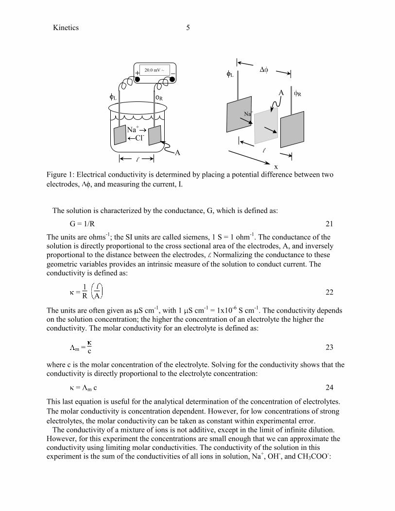
The progress of the reaction is observed using conductivity. Consider a solution with two

electrodes of cross sectional area A, Figure 1. A small potential difference is placed across the

two electrodes, = R – L. The measured current is given by = IR, with R the resistance of

the solution.

Kinetics 5

Figure 1: Electrical conductivity is determined by placing a potential difference between two

electrodes, , and measuring the current, I.

The solution is characterized by the conductance, G, which is defined as:

G = 1/R 21

The units are ohms-1

; the SI units are called siemens, 1 S = 1 ohm-1

. The conductance of the

solution is directly proportional to the cross sectional area of the electrodes, A, and inversely

proportional to the distance between the electrodes, l. Normalizing the conductance to these

geometric variables provides an intrinsic measure of the solution to conduct current. The

conductivity is defined as:

= 1

R l

A 22

The units are often given as S cm-1

, with 1 S cm-1

= 1x10-6

S cm-1

. The conductivity depends

on the solution concentration; the higher the concentration of an electrolyte the higher the

conductivity. The molar conductivity for an electrolyte is defined as:

m = c 23

where c is the molar concentration of the electrolyte. Solving for the conductivity shows that the

conductivity is directly proportional to the electrolyte concentration:

= m c 24

This last equation is useful for the analytical determination of the concentration of electrolytes.

The molar conductivity is concentration dependent. However, for low concentrations of strong

electrolytes, the molar conductivity can be taken as constant within experimental error.

The conductivity of a mixture of ions is not additive, except in the limit of infinite dilution.

However, for this experiment the concentrations are small enough that we can approximate the

conductivity using limiting molar conductivities. The conductivity of the solution in this

experiment is the sum of the conductivities of all ions in solution, Na+, OH

-, and CH3COO

-:

R L

20.0 mV ~ – +

Na+

Cl

-

l A l

A

Na+

R

L

x

Kinetics 6

[Na+] Na+ + [OH

-] OH- + [CH3COO

-] CH3COO- 25

The infinite dilution ionic conductivities of the Na+, OH

-, and CH3COO

- ions are 50.9, 192., and

40.8 S cm2 mol

-1, respectively at 25 C. We can neglect the conductivity of the CH3COO

- ions,

since the molar conductivity of acetate is almost five times smaller than hydroxide. The Na+ ions

contribute a constant background conductivity.

Time Course Data Directly from Conductivities

While the integrated rate law for a reaction is written in terms of the concentration for a given

species, it is often more convenient to plot the experimental data directly. For the initial

conditions, let the initial concentration of OH- be [A]o and the initial concentration of

ethylacetate be [B]o. Ethylacetate will not contribute to the measured conductivity since

ethylacetate is neutral. From Eq. 25 and neglecting the acetate conductivity, the conductivity at

time t is:

= [Na+] Na+ + [OH

-] OH- = [A]o Na+ + ([A]o– ) OH- 26

The initial conductivity at t = 0 is:

o = [Na+]o Na+ + [OH

-]o OH- = [A]o Na+ + [A]o OH- 27

The concentration of OH- at the end of the reaction is determined by the limiting reagent. If OH

-

is the limiting reagent, [A]o<[B]o, and [OH-] = 0 and the solution conductivity at infinite time is:

= [Na+]o Na+ + [OH

-] OH- = = [A]o Na+

(hydroxide limiting: [A]o<[B]o) 28

The following ratio gives the progress of the reaction:

o –

o – =

[A]o (hydroxide limiting: [A]o<[B]o) 29

Eq. 29 can be used to monitor the progress of the reaction directly in curve fitting, bypassing the

necessity of calculating the actual OH- concentration. Then /[A]o is used in curve fitting with

Eqs. 15-17.

Procedure

Equipment:

9x test tubes- 15x150-mm

3x clamps to hold the test tubes in the constant temperature bath

5x rubber stoppers

2x 50-mL volumetric flasks

2x15-mL volumetric pipette

1x5-mL volumetric pipette

Pasture pipette

10-mL beaker

Constant temperature bath set to 35 C.

Vernier LabPro interface and conductivity probe

Kinetics 7

Reagents:

0.020 M NaOH

ethylacetate

Solution Preparation: Make sure to do all solution preparation calculations before you come to

lab. The ethylacetate solution must be prepared just before use, since ethylacetate hydrolyzes in

water at a slow, but appreciable, rate. Prepare a solution of 0.20 0.01 M ethylacetate in water in

a 50-mL volumetric flask. To avoid evaporation, start with some water in the volumetric flask

and then add the ethylacetate. Make sure to record the exact weight of ethylacetate so that you

can calculate the exact concentration to three significant figures. During the first kinetics run also

prepare a 0.05 M solution of ethylacetate in a 50-mL volumetric flask.

Outline: You will do three runs. In the first, sodium hydroxide will be the limiting reagent and

ethylacetate will be in sufficiently large excess that the isolation method applies. In the second

run, ethylacetate will be the limiting reagent with comparable amounts of both reactants. The

third run uses the same conditions as the first, but at a higher temperature, so that the activation

energy and pre-exponential factor may be calculated.

The First Run - Isolation Method: Loosely clamp three dry test tubes into the 35 C constant

temperature bath. Put the conductivity probe into one empty tube so that the probe comes to

constant temperature in the bath. Using a volumetric pipette, transfer 15 mL of the 0.20 M

ethylacetate solution into the second test tube in the bath and stopper to avoid evaporation loss.

Transfer 15 mL of the 0.02 M NaOH solution to the third test tube. Allow the solutions to

equilibrate at the bath temperature.

The instructions for using Logger Pro are in the appendix. Take data points every 15 sec for a

period of 20 minutes or until the conductivity is constant, to within experimental error.

You need to begin data collection as quickly as possible after the solutions are mixed using the

following procedure. Moving as efficiently as possible, remove the test tubes containing the

solutions from the bath. Pour the contents of the tubes together and then pour the combined

solutions back and forth between the two test tubes to ensure complete transfer. Stopper the test

tube and shake vigorously several times to ensure complete mixing, then immediately return the

test tube to the clamp in the bath while immersing the conductivity probe in the solution and

begin data collection.

After this run and each of the following runs, remove the conductivity probe and stopper each

tube with the reaction mixture. Keep the stoppered test tubes in the bath to make sure the reaction

runs to completion. Rinse the conductivity probe with reagent grade water and dry the

conductivity probe with a stream of air from an empty wash bottle to avoid dilution of the next

sample. After you have finished all the other runs, remeasure the conductivity of each reaction

mixture to check the value of . Save each data file and make a printout of each successful run.

If you wish to analyze the data in Excel, pull down the file menu and Export each run to a text

file.

The Second Run – Comparable Amounts of Reactants: For the second run, use 15 mL of 0.050

M ethylacetate and 15 mL of the 0.020 M sodium hydroxide solutions at 35 C. Save each data

file and make a printout of each successful run. Pull down the file menu and export each data to a

text file. You will analyze the data using Excel.

Kinetics 8

The Third Run – Temperature Dependence: Use the same volumes that you used in the first run.

However, run this reaction at 45 C. Save each data file and make a printout of each successful

run. Determine the rate constant using the reaction order that you found at the lower temperature.

Finishing Up–Measuring : After you have finished, don’t forget to remeasure the

conductivity of each reaction mixture to check the value of .

Calculations

For each run use Eq. 29 to calculate /[A]o. Use the value of the conductivity at infinite time, ,

that you measured at the very end of the experiment for each run. For the reaction with

ethylacetate in large excess, plot the data as discussed above for simple one-reactant first and

second order plots, Eqs. 15 and 16. You may use Excel or Logger Pro for the curve fitting.

Determine the reaction order and calculate the rate constant. Include both your first-order and

second-order plots in your report. For the reactions with comparable amounts of reactants, do all

three plots, using Eq. 15, 16 and 17, and determine the overall reaction order and calculate the

rate constant. [If the plot for Eq. 17 has significant curvature, try using the value for from the

last data point in the time course for the reaction instead of the remeasured value after the sample

has sat in the bath for awhile.]

Determine the rate constant at the higher temperature (only one plot is necessary). Determine

the activation energy and the pre-exponential factor using Eq. 20 and 18.

Report

Derive Eq. 29 from Eqs. 26-28 in the Theory section of your report. Provide all the rate constant

data in a tabular format, including all information necessary to repeat your calculations. Make

sure to include the concentrations of hydroxide and ethylacetate for each run. Attach all your

graphs (the five at 35°C and the additional plot for the higher temperature). Report the order of

the reaction with respect to ethylacetate and hydroxide, the rate constant at each temperature, the

activation energy, and pre-exponential factor. Include any slopes and intercepts determined by

curve fitting and the uncertainties. Remember to use propagation of error rules in presenting the

standard deviations in these final rate constants. Since you have only two data points for the

determination of the activation energy, use significant figure rules to report the activation energy

and pre-exponential factor. Discuss the chemical significance of the results. In other words, state

why these results are useful and important. In particular is the proposed mechanism in the

Introduction consistent with your experimentally determine rate law?

References

1. J. Walker, “Method for determining velocities of saponification,” Proc. Roy. Soc. London, ser.

A, 1906, 78, 157-60.

2. F. Daniels, J. W. Williams, P. Bender, R. A. Alberty, C. D. Cornwell, J. E. Harriman,

Experimental Physical Chemistry, 7th

. Ed., McGraw-Hill, New York, NY, 1970. Exp. 23 pp.

144-149.

Kinetics 9

Appendix:

Conductivity and Vernier Data Acquisition Software Instructions

I. Getting Started and Calibration

1. Set the conductivity probe to the 2000 S cm-2

setting before starting Logger Pro. Start

Logger Pro. Logger Pro should recognize the conductivity probe and should begin displaying the

conductivity.

2. Because the ratio in Eq. 26 is unitless, it is not necessary to calibrate the conductivity probe.

However, the probe should read zero when in air or immersed in reagent grade water. If not, with

the probe in air or reagent grade water, pull down the Interface menu and choose zero.

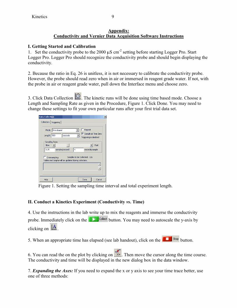
3. Click Data Collection . The kinetic runs will be done using time based mode. Choose a

Length and Sampling Rate as given in the Procedure, Figure 1. Click Done. You may need to

change these settings to fit your own particular runs after your first trial data set.

Figure 1. Setting the sampling time interval and total experiment length.

II. Conduct a Kinetics Experiment (Conductivity vs. Time)

4. Use the instructions in the lab write up to mix the reagents and immerse the conductivity

probe. Immediately click on the button. You may need to autoscale the y-axis by

clicking on .

5. When an appropriate time has elapsed (see lab handout), click on the button.

6. You can read the on the plot by clicking on . Then move the cursor along the time course.

The conductivity and time will be displayed in the new dialog box in the data window.

7. Expanding the Axes: If you need to expand the x or y axis to see your time trace better, use

one of three methods:

Kinetics 10

Automatic scaling: Click on the Autoscale icon .

Using the cursor: Position the cursor over the axis you want to expand. The cursor will

change shape, Figure 2. Drag the mouse to change the scale expansion.

Figure 2. Move the cursor over the axis to change the axis scale.

Direct input: Click near the maximum or minimum of the axis you want to change. A dialog

box will appear, Figure 3, and you can the type in the value that you want for the scale limit.

Figure 3. Click near the axis maximum or minimum to show the dialog box.

8. Save the data file to the disk by pulling down the file menu and choosing Save As… Save

your data files to the Documents directory.

9. Pull down the file menu and choose Export. Export the data to a text file, again in the

Documents directory.

10. Pull down the Data menu and choose Clear All Data.

11. Set up another run. Return to step 4. If you forget to Clear All Data, you will get a dialog box:

Choose Erase and Continue.

IV. Finishing up

1. Make sure to wash all your glassware. Sodium hydroxide solutions etch glass over time.

Kinetics 11

2. Make sure the area around the apparatus is clean and dry. Leave the conductivity probe to dry

in air.

3. Transfer your text files to the server.

4. Log off of the computer.

Kinetic Data Analysis Using Vernier Software.

Outline: The progress of the reaction using the isolation method is calculated using Eq. 29 to

find:

1 – /[A]o = 1 – o –

o –

You can then use the built in plotting facilities in Logger Pro to do the time course plots, Eq. 15-

16, or you can use Excel. The time course plots are often done using [A] as the concentration

variable, as in Eqs. 7 and 9. So the instructions below are specified using that variable name for

generality. Please note that care must be taken to avoid zero or negative values, since the logarithm of zero or a negative number is undefined. LoggerPro skips these points in its plots, so your plot may be worse than it appears when some of the points are missing.

1. Use the first data point as o and your final measurement as . Alternatively, for a quick

analysis, just use the smallest conductivity from the time course for . In the example

below, we will assume o = 3230 S cm-1

and = 1786 S cm-1

, just to have some numbers

to use. b. Choose New Calculated Column from the Data menu.

c. Enter “A” as the Name, “A” as the Short Name, and leave the unit blank. The value of

(1 – /[A]o) is unitless.

d. Enter the formula = 1 – o –

o – for the column into the Equation edit box. For the at

time t, choose “Conductivity” from the Variables pull down list. In the Equation edit box,

you should now see displayed something like "1-(3230-“Conductivity”)/(3230-1786)” Click .

e. Click on the y-axis label. Choose “A.” A graph of corrected absorbance vs. time should

now be displayed.

2. Follow these directions to create a calculated column, ln A, and then plot a graph of ln A vs.

time:

a. Choose New Calculated Column from the Data menu.

b. Enter “ln A” as the Name, “ln A” as the Short Name, and leave the unit blank. A logarithm is always unitless.

c. To enter the correct formula for the column into the Equation edit box, choose “ln” from

the Function list. Then select “A” from the Variables list. In the Equation edit box, you

should now see displayed: ln(“A”). Click .

Kinetics 12

d. Select Additional Graphs Strip Chart from the Insert menu. Click on the y-axis label in

this new Strip Chart. Choose ln A. A graph of ln absorbance vs. time should now be

displayed. Autoscale the y-axis by clicking on . To see if the relationship is linear,

click the Linear Fit button, .

e. You will probably have some values in the long time portion that will make it difficult to

get a useful vertical axis scale. To avoid plotting these points, in the data table scroll down

to the bottom of the table and locate the first negative A value. Click on the row number

one or two rows before the first negative A value. Then shift click on the last row in the

data table. Pull down the edit menu and choose “Strike Through Data Cells.” Those

chosen cells will no longer be plotted and Autoscaling the plot should work better to help

you set the vertical axis expansion, Figure 4. You can also select rows in the data table by

using the mouse to drag over the corresponding range in the data plot.

a. b.

Figure 4. (a) Noisy points at the long-time end cause a large scale range. (b) The Strike

Through Data Cells option is used to avoid plotting and fitting values at the end of the

kinetics run where noise dominates. Notice the scale is expanded almost by a factor of two

with the last several points omitted from the plot.

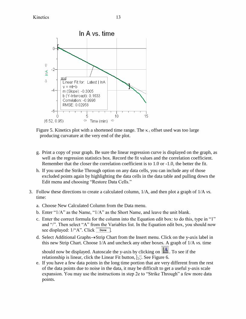
f. The very long-time behavior of your plot may be noisy and may have some curvature,

Figure 5. This curvature may be caused by not knowing the exact . You can narrow the

range for the linear curve fit by dragging the ] at the right-hand side of the plot. However,

keep the fitting interval as wide as possible. (If the ] handle isn’t showing, remove the

current curve and fit again.) Use the same time interval when comparing the curve fit for

the 1/A vs. time plot, to make a fair comparison. Alternatively, you can adjust the value

in the calculation for the A column to get a longer linear range. You can edit the formula

for a column by double clicking the column label in the data table. Adjusting the offset

also makes a fair comparison, since the same offset is used in both curve fits. However,

make sure that this infinite time value makes sense (i.e. estimate by eye and check your

result). Choosing an incorrect value can distort the data plots so that you end up

choosing the incorrect order.

Kinetics 13

Figure 5. Kinetics plot with a shortened time range. The offset used was too large

producing curvature at the very end of the plot.

g. Print a copy of your graph. Be sure the linear regression curve is displayed on the graph, as

well as the regression statistics box. Record the fit values and the correlation coefficient.

Remember that the closer the correlation coefficient is to 1.0 or -1.0, the better the fit.

h. If you used the Strike Through option on any data cells, you can include any of those

excluded points again by highlighting the data cells in the data table and pulling down the

Edit menu and choosing “Restore Data Cells.”

3. Follow these directions to create a calculated column, 1/A, and then plot a graph of 1/A vs.

time:

a. Choose New Calculated Column from the Data menu.

b. Enter “1/A” as the Name, “1/A” as the Short Name, and leave the unit blank.

c. Enter the correct formula for the column into the Equation edit box: to do this, type in “1”

and “/”. Then select “A” from the Variables list. In the Equation edit box, you should now

see displayed: 1/“A”. Click .

d. Select Additional Graphs Strip Chart from the Insert menu. Click on the y-axis label in

this new Strip Chart. Choose 1/A and uncheck any other boxes. A graph of 1/A vs. time

should now be displayed. Autoscale the y-axis by clicking on . To see if the

relationship is linear, click the Linear Fit button, . See Figure 6.

e. If you have a few data points in the long time portion that are very different from the rest

of the data points due to noise in the data, it may be difficult to get a useful y-axis scale

expansion. You may use the instructions in step 2e to “Strike Through” a few more data

points.

Kinetics 14

f. When you compare the ln A and 1/A plots, use the same time interval for your linear fit as

you did for the ln A fit. Make sure to expand the y scale so the y-values during the chosen

time interval cover the full y-axis. In other words, the long time y-values can be off scale.

By greatly expanding the y-axis, Figure 6b, you will be better able to judge the linearity

over the chosen time interval in a comparable scale expansion to your ln A vs. t plot.

a. b.

Figure 6. (a.) The y-axis range is too large because of noisy points at the long-time end. (b.)

Expand the y-axis scale to get a comparable view to the ln A vs. t plot (compare with

Figure 9 at right).

g. Print a copy of your graph. Include this graph in your report. Be sure the linear regression

curve is displayed on the graph, as well as the regression statistics box. Record the fit

values and the correlation coefficient.

4. Copies of the plots should be in both partners’ lab notebooks. Report the order and rate

constant, k. Make sure to include both ln A vs. t and 1/A vs. t plots in your report, since the

comparison between the two plots determines the proper order.