kathryn wheel a_spectacular_galaxy_collision_discoverd_in_the_galactic_neighbourhood
TRANSCRIPT
MNRAS 452, 3759–3775 (2015) doi:10.1093/mnras/stv1432
Kathryn’s Wheel: a spectacular galaxy collision discoveredin the Galactic neighbourhood
�
Quentin A. Parker,1,2† Albert A. Zijlstra,3† Milorad Stupar,4 Michelle Cluver,5
David J. Frew,1 George Bendo3 and Ivan Bojicic1
1Department of Physics, Chong Yuet Ming Physics Building, The University of Hong Kong, Hong Kong2Australian Astronomical Observatory, PO Box 915, North Ryde, NSW 1670, Australia3Jodrell Bank centre for Astrophysics, School of Physics and Astronomy, University of Manchester, Oxford Road, Manchester M13 9PL, UK4University of Western Sydney, Locked Bag 1797, Penrith South, DC, NSW 1797, Australia5University of the Western Cape, Robert Sobukwe Road, Bellville 7535, South Africa
Accepted 2015 June 24. Received 2015 June 15; in original form 2015 May 7
ABSTRACTWe report the discovery of the closest collisional ring galaxy to the Milky Way. Such raresystems occur due to ‘bulls-eye’ encounters between two reasonably matched galaxies. Therecessional velocity of about 840 km s−1 is low enough that it was detected in the Anglo-Australian Observatory/UK Schmidt Telescope Survey for Galactic H α emission. The distanceis only ∼10 Mpc and the main galaxy shows a full ring of star-forming knots, 6.1 kpcin diameter surrounding a quiescent disc. The smaller assumed ‘bullet’ galaxy also showsvigorous star formation. The spectacular nature of the object had been overlooked because ofits location in the Galactic plane and proximity to a bright star and even though it is the 60thbrightest galaxy in the HI Parkes All Sky Survey (HIPASS) H I survey. The overall system hasa physical size of ∼15 kpc, a total mass of M∗ = 6.6 × 10⁹ M� (stars + H I), a metallicityof [O/H]∼ −0.4, and a star formation rate of 0.2–0.5 M� yr−1, making it a Magellanic-type system. Collisional ring galaxies therefore extend to much lower galaxy masses thancommonly assumed. We derive a space density for such systems of 7 × 10⁻⁵ Mpc−3, an orderof magnitude higher than previously estimated. This space density suggests Kathryn’s Wheelis the nearest such system. We present discovery images, CTIO 4-m telescope narrow-bandfollow-up images and spectroscopy for selected emission components. Given its proximityand modest extinction along the line of sight, this spectacular system provides an ideal targetfor future high spatial resolution studies of such systems and for direct detection of its stellarpopulations.
Key words: galaxies: groups: general – galaxies: individual (ESO 179-13) – galaxies:interactions – galaxies: kinematics and dynamics – galaxies: star formation.
1 IN T RO D U C T I O N
Among the structures shown by interacting galaxies (Barnes &Hernquist 1992), the so-called collisional ring galaxies (Theys &Spiegel 1976, 1977) are a rare and most distinctive sub-class (Apple-ton & Struck-Marcell 1996). Collisional ring galaxies occur from analmost head-on collision between a smaller galaxy travelling alongthe minor axis of a larger galaxy passing through, or close to, its cen-tre (Appleton & Struck-Marcell 1996). The shock wave sweeps upand expels gas from the system, usually leaving a gas-poor galaxybehind (Freeman & de Vaucoleurs 1974).
�Named after the wife of the second author.†E-mail: [email protected] (QAP); [email protected] (AAZ)
The pre-eminent example is the Cartwheel galaxy (ESO 350-40; AM 0035-335) at a distance of 124 Mpc. The Cartwheel wasdiscovered by Zwicky (1941), and studied in-depth by Fosbury &Hawarden (1977) and Amram et al. (1998). The Cartwheel showsa spectacular ring of star formation, with interior spokes surround-ing the host galaxy. Other well-known collisional systems includeArp 148 (Mayall’s Object) at 148 Mpc (Smith 1941; Burbidge, Bur-bidge & Prendergast 1964; Arp 1966), IC 298 (Arp 147; Gerber,Lamb & Balsara 1992) at 135 Mpc, and AM 0644-741 (ESO 34-11 or the ‘Lindsay–Shapley Ring’) at 87 Mpc (Lindsay & Shapley1960; Graham 1974; Arp & Madore 1987). This latter object is of-ten considered to be a typical exemplar of evolved ringed galaxies(e.g. Higdon, Higdon & Rand 2011).
While star-forming events resulting from galactic collisions maybe more common than usually thought (e.g. Block et al. 2006),
C© 2015 The AuthorsPublished by Oxford University Press on behalf of the Royal Astronomical Society
by guest on August 17, 2015
http://mnras.oxfordjournals.org/
Dow
nloaded from
3760 Q. A. Parker et al.
spectacular cartwheel-type galaxies, showing complete rings (butnot necessarily with evident spokes), appear to be very rare involume-limited surveys. The previous nearest example was the VelaRing galaxy (AM 1006-380 = ESO 316-43), at 72 Mpc (Dennefeld,Lausten & Materne 1979). Partial ring galaxies are more numerous.Probably the nearest in the Madore, Nelson & Petrillo (2009) cata-logue is AM 0322-374 at 20 Mpc. UGC 9893, at 11 Mpc (Kennicuttet al. 2008), is also listed as a collisional system, but it lacks a clearring structure (Gil de Paz, Madore & Pevunova 2003), appearingindistinct in available imagery. Collisional ring galaxy systems canbe identified in high-resolution, deep H α imagery where the H II
regions of the ring are readily visible. However, H α galaxy surveyssuch as Gil de Paz et al. (2003), James et al. (2004), and Kennicuttet al. (2008) have not added to the modest number of cartwheel-typegalaxies currently known and there are <20 convincing systems, e.g.Marston & Appleton 1995. Brosch et al. (2015) present the mostrecent detailed work on such systems for an apparently empty ringgalaxy system ESO 474 G040 at ∼78 Mpc, thought to have arisenfrom a recent merger of two disc galaxies.
Collisional rings systems offer an excellent environment tostudy the evolution of density-wave-induced starbursts (Marston &Appleton 1995; Romano, Mayya & Vorobyov 2008), as well as thedynamic interactions between the individual galaxies (e.g. Smithet al. 2012). A closer example of a collisional ring system wouldallow its star formation, stellar distribution, and evolution to be stud-ied in detail, spatially, kinematically and chromatically. Here, wepresent the discovery of a new collisional ring galaxy at a distanceof only 10 Mpc. Our paper is organized as follows. In Section 2,we present some background and describe the discovery of thering around ESO 179-13. In Section 3, we present our follow-uphigh-resolution imaging and other archival multiwavelength im-ages. Optical spectroscopy is presented in Section 4. Parametersfor the system, such as masses and star formation rates (SFR), areprovided in Section 5. Section 6 presents our discussion and givesour summary in Section 7.
2 BAC K G RO U N D A N D D I S C OV E RY
2.1 Background
ESO 179-13 is noted as an interacting double galaxy system inSIMBAD, appearing to consist of a near edge-on late-type spi-ral with another more chaotic system ∼80 arcsec to the north-east. It was first identified by Sersic (1974) and independentlyre-discovered by Lauberts (1982), Longmore et al. (1982) andCorwin, de Vaucouleurs & de Vaucouleurs (1985). A detailedB-band image was published by Laustsen, Madsen & West (1987).
Woudt & Kraan-Korteweg (2001) identify the most prominentgalaxy as WKK 7460 (component A hereafter), and WKK 7463 forthe secondary (component B). A small, third galaxy is also identifiedas WKK 7457 to the west of component A (component C). It agreeswith our own positional determination to 1 arcsec. The system,centred on component A, is entry 391 in the H α catalogue ofKennicutt et al. (2008), but they do not list integrated H α (+ [N II])flux or luminosity estimates. Lee et al. (2011), in a related paper,included this system in their Galaxy Evolution Explorer (GALEX)ultraviolet (UV) imaging survey of local volume galaxies with aquoted BT = 15, but no near-UV or far-UV fluxes are quoted.Owing to its proximity to the Galactic plane, the galaxy was notobserved by GALEX prior to mission completion (Bianchi 2014).
Component A has been classified as an SB (s) m spiral in theRC3 catalogue (de Vaucouleurs et al. 1991) and similarly classified
as SB (s) dm system (T = 7.5) by Buta (1995). These independentclassifications treat the system as a distinct, late-type spiral galaxy,albeit in an interaction. It can be best described as a Magellanicdwarf or a Magellanic spiral, similar to the Large Magellanic Cloud(LMC).
A range of heliocentric radial velocities for component A areavailable in the literature from both optical spectroscopic and H I
measurements. The most recent optical results are Strauss et al.(1992) who quote 775 ± 36 km s−1, Di Nella et al. (1997),750 ± 70 km s−1, and Woudt, Kraan-Korteweg & Fairall (1999),757 ± 50 km s−1. These are in good agreement so we take an un-weighted average of 761 km s−1 (σ = 11 km s−1) for component A.
The earliest H I heliocentric velocities towards the system are836 ± 5 km s−1 by Longmore et al. (1982), 840 ± 20 km s−1
by Tully (1988) and 843 ± 9 km s−1 by de Vaucouleurs et al.(1991). The Parkes H I ‘HIPASS’ Multibeam receiver programmegives 843 ± 5 km s −1 (HIPASS catalogue; Meyer et al. 2004),where it is noted as the 60th brightest in terms of integrated fluxdensity (Koribalski et al. 2004). A deeper, pointed Parkes observa-tion was obtained by Schroder, Kraan-Korteweg & Henning (2009).They give parameters for component A, but note that a contributionfrom component B is likely. Their heliocentric H I radial velocity is842 km s−1 from the H I profile mid-point, with a velocity width of222 km s−1 at 20 per cent of peak. The integrated H I flux densityis 113.8 ± 3.7 Jy km s−1, in good agreement with the HIPASSvalue of 100. All the H I velocities are consistent within small errors.These values include the combined contribution from all the gas inthe full system. We adopt 842 ± 5 km s−1 for the combined H I
system velocity.Kennicutt et al. (2008) give a distance of 9 Mpc based on a Vir-
gocentric flow model distance. We adopt a slightly further distanceof 10.0 ±1.0 Mpc, based on Kennicutt et al. (2008), but scalingfrom a Hubble constant H0 of 75 to 68 km s−1 Mpc−1 due to the lat-est Wilkinson Microwave Anisotropy Probe (Hinshaw et al. 2013)and Planck results (Ade et al. 2014). At this distance, 1 arcsecequates to 48.5 pc. Woudt & Kraan-Korteweg (2001) gives a mod-est colour excess of E(B−V) = 0.25 mag in the surrounding field,giving AV = 0.78 mag, while Schlafly & Finkbeiner (2011) giveAV = 0.75 mag for Galactic extinction in this general direction,which we adopt hereafter. We will also use AHα = 0.61 mag basedon the reddening law from Howarth (1983).
Apart from the basic information above, the system has beenlittle studied because of its location in a crowded, low-latitude areanear the Galactic plane (|b| = −8◦) and proximity to the bright,7.7 mag A0 IV star, HD 150915, located 72 arcsec due south. Thereare actually two bright stars here, but only HD 150915 is listed inSIMBAD. The second star is ∼10 arcsec north of HD 150915 and∼2 mag fainter. It was undoubtedly blended with HD 150915 inthe original photographic imagery.
2.2 Discovery of the ring
The low heliocentric velocity meant the system was discovered asa strong H α emitter in the Anglo-Australian Observatory (AAO) /UK Schmidt Telescope (UKST) SuperCOSMOS H α survey of theSouthern Galactic Plane (SHS; Parker et al. 2005) during searchesfor Galactic planetary nebulae (Parker et al. 2006). The bandpassof the survey filter (Parker & Bland-Hawthorn 1998) includes allvelocities of Galactic gas and emission from extragalactic objectsout to the Virgo and Fornax galaxy clusters at ∼1200 km s−1.
Fig. 1 shows the 4 × 4 arcmin discovery images from the SHSsurvey data centred on the system. From left to right there is the
MNRAS 452, 3759–3775 (2015)
by guest on August 17, 2015
http://mnras.oxfordjournals.org/
Dow
nloaded from
The nearest collisional ring galaxy 3761
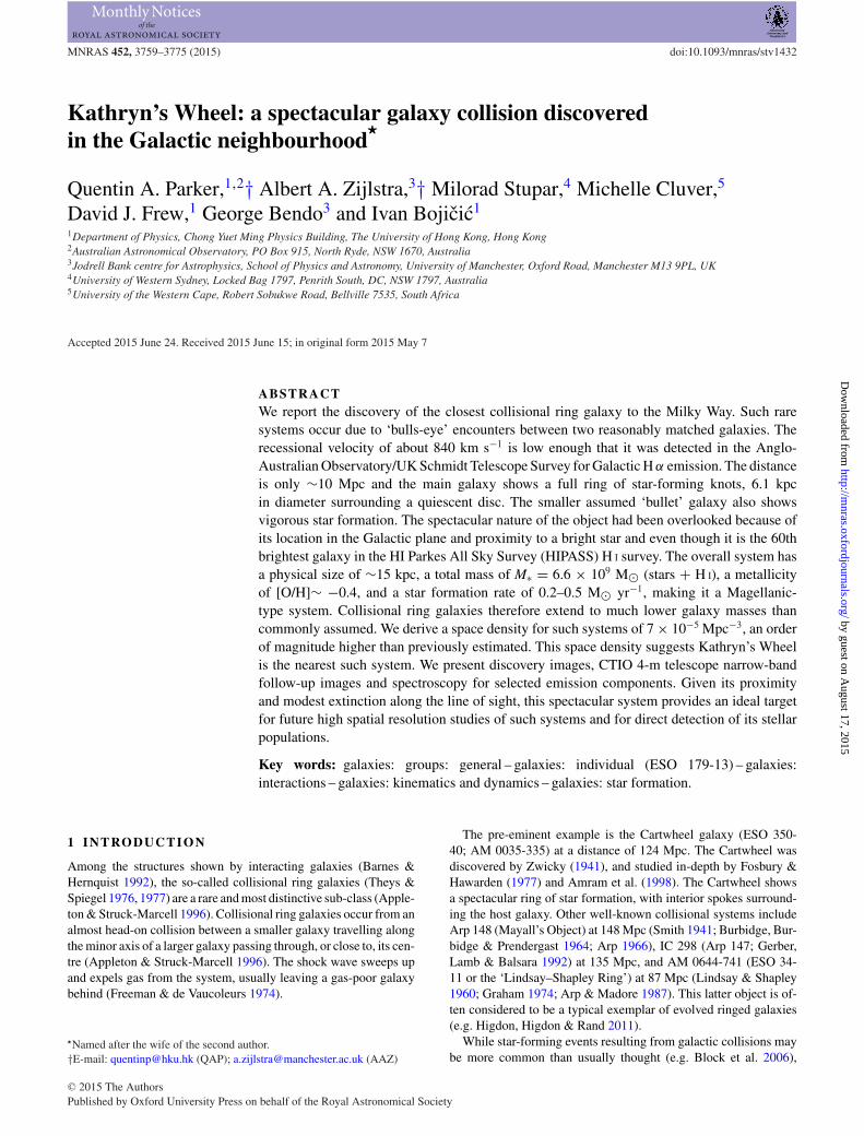
Figure 1. Left-hand panel: The 4 × 4 arcmin SHS broad-band short-red ‘SR’ image centred on component A at 16h47m19.s7, −57◦26′31′ ′ (J2000). Northis top and east left. Mid panel: The matching H α image. Right-hand panel: The continuum-subtracted image obtained by taking the SR from the SHS H α
(+ [N II]) image scaled at 99.5 per cent. North is at the top and east to the left. Component B is labelled to the north-east and component C is indicated with anarrow.
H α image, the matching broad-band short-red ‘SR’ image andthe image obtained by taking the SR image from the H α image(effectively a continuum-subtracted image). Component A is at thecentre. Component B is labelled to the north-east, while the smallercompact component C is indicated with an arrow.
The SHS continuum-subtracted image reveals a spectacular ringof emission knots not obvious, without context, even in the H α
image, while the main component A galaxy has almost disap-peared. The ring is approximately (but not perfectly) centred oncomponent A. Surprisingly, given its previous spiral morphologi-cal classification, component A does not show up well in the SHScontinuum-subtracted image and appears to show little star forma-tion. This indicates that along with its apparently highly elongatednature (so not an elliptical) it is has been largely stripped of gas.The smaller, more irregular galaxy (component B), which we as-sume is the bullet that impacted the target galaxy, component A,shows extensive, clumpy H α emission. A third, faint compact sys-tem (component C) is seen 38 arcsec to the west of component A,identified as WKK 7457. This object is clear in the broad-bandB-, R-, and I-band SuperCOSMOS images and is also undergoingstar-formation.
The strong H I detection noted earlier indicates that a significant,neutral H I component still remains within the overall system envi-ronment. The lack of much star formation in component A suggeststhat most of this H I may be located outside of its inner disc.
3 FO L L OW-U P I M AG I N G A N DM U LT I WAV E L E N G T H C O M PA R I S O N S
Discovery of this collisional ring system led us first to investigateand compile existing multiwavelength data from the archives. Wethen obtained deeper, higher resolution imaging and spectroscopyof the major emission components (see below), to provide estimatesof some key physical parameters for this system.
3.1 CTIO 4-m-telescope imaging
High-resolution imagery at the Blanco 4-m telescope at CTIO wasobtained in 2008 June using the wide field mosaic camera. We usedfive filters: V-band, Hα, H α off-band (80Å redward of H α), [O III] ,and a (wider) [O III] off-band filter centred at 5300Å. The field of
view is 30 arcmin on a side and the plate scale 0.26 arcsec px−1.The seeing measured from the data frames was typically 1.2 arcsec.Exposures were 5 min for the emission-line and off-band filters,and 60 s for the V-band filter. The airmass during the exposuresaveraged 1.3. To subtract the continuum, the H α off-band imagewas scaled down by a factor of 0.88, and the [O III] off-band by afactor of 0.14, to compensate for the filter widths. These factors wereestablished by minimizing residuals for a set of selected field stars.For [O III] that works very well and results are in good agreementwith the filter curve. For H α this can be an issue if the chosen starshave H α in absorption. This does not appear to be the case for thefield stars chosen which provide a consistent scale-factor to ∼2 percent. It is best to minimize stellar residuals rather than filter curvesas stars are a more important contribution to the continuum thanbound-free emission from H I regions.
A montage of these CTIO images is shown in Fig. 2. They revealthe distribution and variety of the emission structures as well as datafor quantitative flux estimates. From these deeper, higher resolutionCTIO H α and [O III] continuum-subtracted images, the distributionof ionized gas is seen to be far more complex than is evident fromthe SHS discovery data.
The leftmost panel is a 3 × 3 arcmin CTIO H α image with theoff-band frame subtracted. We avoid the bright star to the southwhere CCD blooming is serious. Emission associated with com-ponent C and at the southern tip of component A’s disc previouslygave the impression of a circular ring in the SHS as the bright starobscured emission further south. The higher resolution CTIO datareveals an elliptical emission ring with a major-axis diameter of127 arcsec (∼6.2 kpc). The inscribed oval was positioned to fit theprominent emission now seen to extend further south. The ellipseis not centred on component A, but at 16h47m19.s5, −57◦26′44′′
(J2000), ∼13 arcsec (or ∼0.6 kpc) south-south-east. Some low-level H α emission is now seen across component A, surroundingcomponent B and with faint, localized emission features and blobsaround the entire system. An interesting feature is the elongated na-ture of some of these emission knots in a north-east direction fromA to B. The main [O III] emission features follow the equivalentH α structures though at typically a third to a half of their nativeintegrated pixel intensities.
The mid panel is the matching CTIO continuum-subtracted[O III] image (narrow on and off-band [O III] images used). Both
MNRAS 452, 3759–3775 (2015)
by guest on August 17, 2015
http://mnras.oxfordjournals.org/
Dow
nloaded from
3762 Q. A. Parker et al.
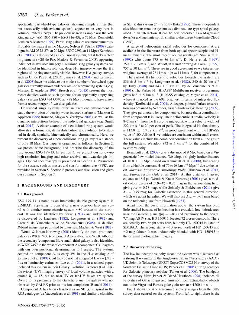
Figure 2. Selected 3 × 3 arcmin regions from the CTIO 4-m imaging centred at 16h47m21s, − 57◦26′03′ ′ (J2000). Left-hand panel: the CTIO continuum-subtracted H α. The green oval has a major axis diameter of 127 arcsec (∼6.2 kpc) and a minor axis of 91 arcsec (∼4.4 kpc). Mid panel: matching CTIOcontinuum-subtracted [O III] image. Both these images are at 90 per cent scaling to better reveal the emission otherwise the 7.7th magnitude star dominates.Right-hand panel: CTIO [O III] off-band image. This represents the V-band starlight without any [O III] and Hβ emission line contribution. Dust lanes can beclearly seen at the southern tip of component A. The more diffusely distributed starlight can also be seen in and around components A and B.
these images are presented at 90 per cent linear scaling to revealthe full extent of the emission (this sets the upper and lower limitsbased on the 90 per cent pixel intensity level where a histogram ofthe data is created and the limits are set to display the percentageabout the mean value). With full pixel range, saturated pixels fromthe 7.7th magnitude star HD 150915 would prevent detail beingseen. Low-level diffuse [O III] flux is seen for component A, but itis not conspicuous. This shows it has almost been completely can-celled out indicating component A is mostly composed of normalstarlight.
The right-hand panel is the off-band [O III] filter image(5300Å) that effectively represents the V-band starlight without the[O III] +Hβ emission line contribution. This shows dust lanes alongand at the south-west extremity of the disc, concentrated starlightfrom components A, B, and C and an envelope of diffuse starlightaround the entire system. This ‘common envelope’ was alreadynoted by Laustsen et al. (1987) from old B-band photographic datataken with the ESO 3.6-m telescope in the 1980s. This raises aninteresting question and also a possible explanation for why the ap-parent axial ratios of the highly elongated component A differs somuch from the surrounding oval ring. Currently known collisionalring systems with low-impact parameter have axial ratios that arebroadly similar to that of the target galaxy. Such arrangements area natural consequence of the copious gas and interstellar mediumbeing swept up and compressed by the resultant density wave hav-ing a similar radial (and perhaps also vertical) distribution as thetarget galaxy stellar content. This does not appear to be the casehere unless what we are actually seeing is the residual, less-inclinedbar of a more face-on disc system that extends out to the entirering and whose presence can still be seen in the low-level diffusestarlight refereed to earlier. If component A is not a residual barbut a distinct late-type disc galaxy (as commonly assumed) strippedof gas, then the gas distribution could have become less flattenedsomehow. Alternatively the original target galaxy could have beenstretched out along the direction of the impact towards compo-nent B before, during, or even after the bulls-eye collision occurred.Though component B is only 13 per cent of the mass (in stars) ofcomponent A, these effects could have been strengthened due to thelow ‘Magellanic’-type masses of the system as a whole.
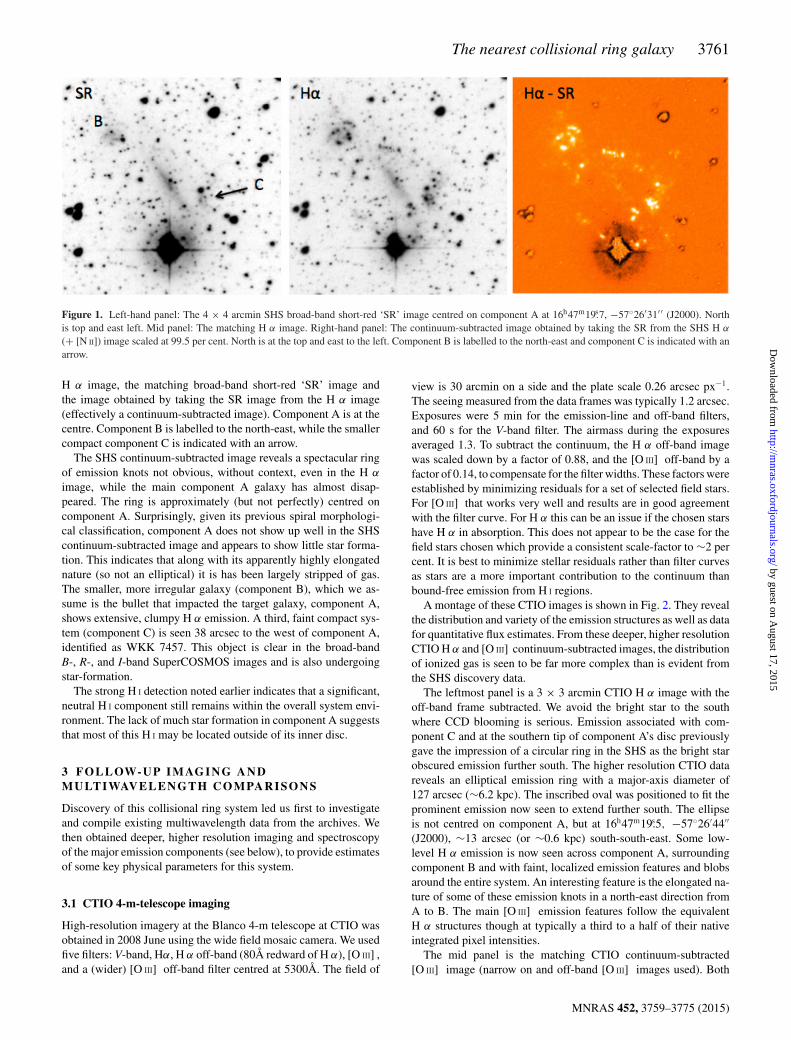
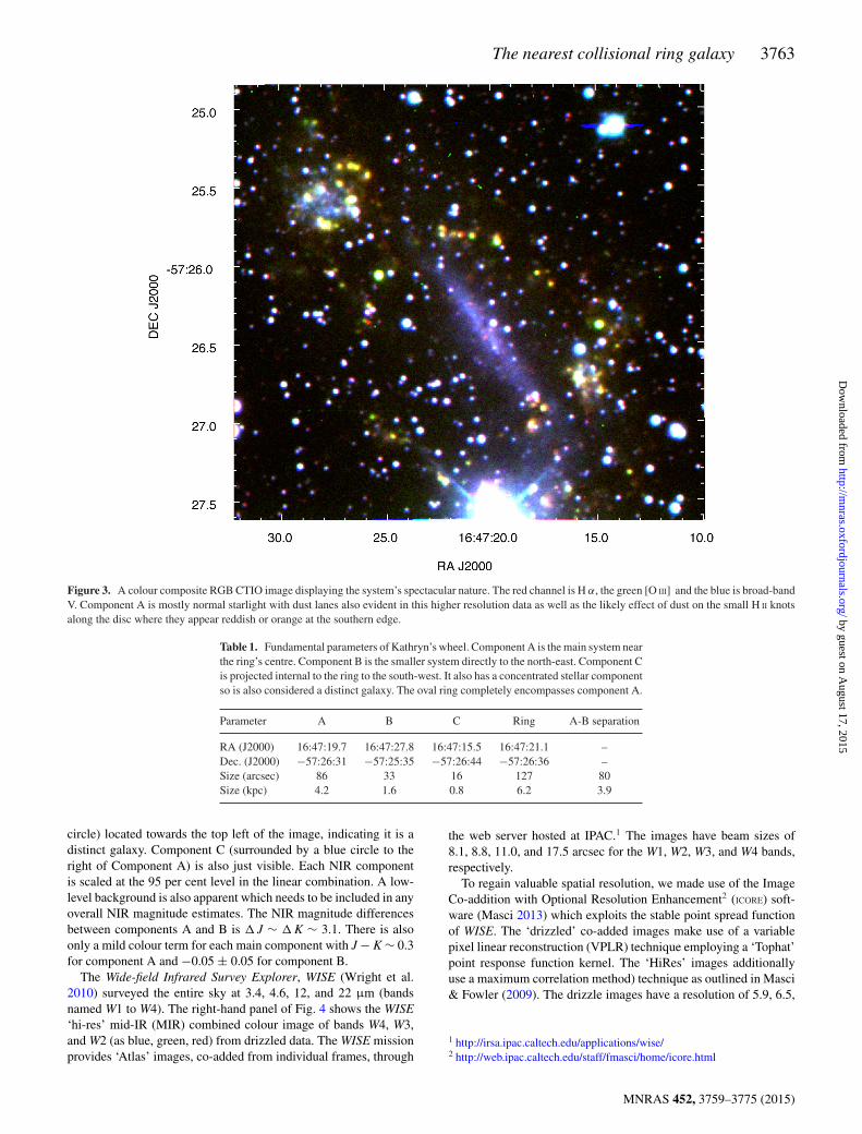
Finally, Fig. 3 is a composite Red, Green, Blue (RGB) CTIOimage displaying the system’s spectacular nature. The red channel
is H α, the green [O III] and the blue broad-band V. Component A ismostly starlight with dust lanes evident in this higher resolution data.The few small H II knots appear red, likely due to dust extinctionwithin the disc.
Based on the SHS data, literature data, and our new CTIO images,Table 1 presents some key parameters for galaxy components A,B, and C, including the central position of the best-fitting ellipseto the main emission ring. The position for component A is tied tothe 2MASS (Skrutskie et al. 2006) near-infrared (NIR) imagery andastrometry. The positions refer to the centre of each assumed galaxy.The centre of component A is derived from the dominant starlightin the R band. The separation between the centres of components Aand B is ∼80 arcsec. Using the distance of 10 Mpc gives a projectedseparation between them of 3.9 kpc.
Component A has a major-axis of ∼86 arcsec (4.2 kpc) measuredto the outer edge in the stellar continuum from off-band [O III] andV-band CTIO images, where a decline in the background is seenbefore the star-forming ring is encountered. When checked againstthe broad-band R, I and 2MASS images when autocut at the90 per cent pixel intensity level, the disc appears to extend onlyto 70–80 arcsec. At low isophotal thresholds, starlight extends outto the star-forming ring both along the major and minor axes. Com-ponent B has a major axis of ∼33 arcsec (1.6 kpc) determined inthe same way. The strongest H α emission in B is also in an ovalstructure of nucleated knots ∼32 arcsec across. This is in excellentagreement with the value estimated from the concentrated starlight.Starlight internal to this emission oval is clear in Fig. 3 and B mayextend to 70 arcsec (∼3.4 kpc) in low level, isolated clumps of starformation and diffuse starlight.
The overall system envelope, including all assumed associatedbroad and narrow band emission and diffuse starlight as seen acrossthe region in the right-hand panel of Fig. 2, has a major diameterof 318 arcsec and a minor axis of 198 arcsec, giving a total systemsize of ∼15.4 × 9.6 kpc.
3.2 Near and mid infrared imaging
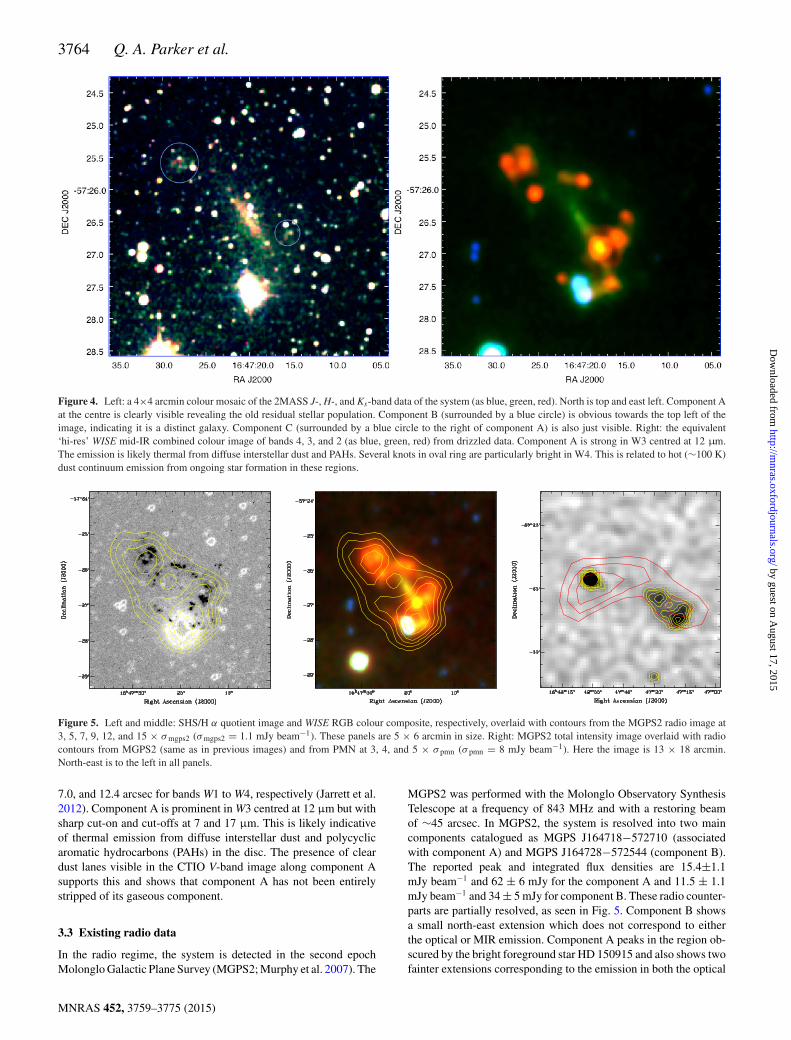
The 2MASS colour combined J-, H-, and Ks-band image (as red,green, blue) is presented in the left-hand panel of Fig. 4. The oldstellar population of component A is clear in the NIR and seento be well separated from component B (surrounded by a blue
MNRAS 452, 3759–3775 (2015)
by guest on August 17, 2015
http://mnras.oxfordjournals.org/
Dow
nloaded from
The nearest collisional ring galaxy 3763
Figure 3. A colour composite RGB CTIO image displaying the system’s spectacular nature. The red channel is H α, the green [O III] and the blue is broad-bandV. Component A is mostly normal starlight with dust lanes also evident in this higher resolution data as well as the likely effect of dust on the small H II knotsalong the disc where they appear reddish or orange at the southern edge.
Table 1. Fundamental parameters of Kathryn’s wheel. Component A is the main system nearthe ring’s centre. Component B is the smaller system directly to the north-east. Component Cis projected internal to the ring to the south-west. It also has a concentrated stellar componentso is also considered a distinct galaxy. The oval ring completely encompasses component A.
Parameter A B C Ring A-B separation
RA (J2000) 16:47:19.7 16:47:27.8 16:47:15.5 16:47:21.1 –Dec. (J2000) −57:26:31 −57:25:35 −57:26:44 −57:26:36 –Size (arcsec) 86 33 16 127 80Size (kpc) 4.2 1.6 0.8 6.2 3.9
circle) located towards the top left of the image, indicating it is adistinct galaxy. Component C (surrounded by a blue circle to theright of Component A) is also just visible. Each NIR componentis scaled at the 95 per cent level in the linear combination. A low-level background is also apparent which needs to be included in anyoverall NIR magnitude estimates. The NIR magnitude differencesbetween components A and B is � J ∼ � K ∼ 3.1. There is alsoonly a mild colour term for each main component with J − K ∼ 0.3for component A and −0.05 ± 0.05 for component B.
The Wide-field Infrared Survey Explorer, WISE (Wright et al.2010) surveyed the entire sky at 3.4, 4.6, 12, and 22 µm (bandsnamed W1 to W4). The right-hand panel of Fig. 4 shows the WISE‘hi-res’ mid-IR (MIR) combined colour image of bands W4, W3,and W2 (as blue, green, red) from drizzled data. The WISE missionprovides ‘Atlas’ images, co-added from individual frames, through
the web server hosted at IPAC.1 The images have beam sizes of8.1, 8.8, 11.0, and 17.5 arcsec for the W1, W2, W3, and W4 bands,respectively.
To regain valuable spatial resolution, we made use of the ImageCo-addition with Optional Resolution Enhancement2 (ICORE) soft-ware (Masci 2013) which exploits the stable point spread functionof WISE. The ‘drizzled’ co-added images make use of a variablepixel linear reconstruction (VPLR) technique employing a ‘Tophat’point response function kernel. The ‘HiRes’ images additionallyuse a maximum correlation method) technique as outlined in Masci& Fowler (2009). The drizzle images have a resolution of 5.9, 6.5,
1 http://irsa.ipac.caltech.edu/applications/wise/2 http://web.ipac.caltech.edu/staff/fmasci/home/icore.html
MNRAS 452, 3759–3775 (2015)
by guest on August 17, 2015
http://mnras.oxfordjournals.org/
Dow
nloaded from
3764 Q. A. Parker et al.
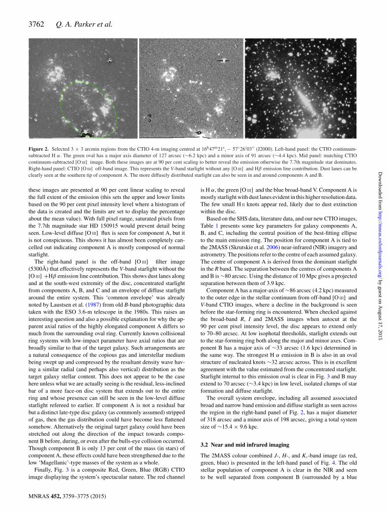
Figure 4. Left: a 4×4 arcmin colour mosaic of the 2MASS J-, H-, and Ks-band data of the system (as blue, green, red). North is top and east left. Component Aat the centre is clearly visible revealing the old residual stellar population. Component B (surrounded by a blue circle) is obvious towards the top left of theimage, indicating it is a distinct galaxy. Component C (surrounded by a blue circle to the right of component A) is also just visible. Right: the equivalent‘hi-res’ WISE mid-IR combined colour image of bands 4, 3, and 2 (as blue, green, red) from drizzled data. Component A is strong in W3 centred at 12 µm.The emission is likely thermal from diffuse interstellar dust and PAHs. Several knots in oval ring are particularly bright in W4. This is related to hot (∼100 K)dust continuum emission from ongoing star formation in these regions.
Figure 5. Left and middle: SHS/H α quotient image and WISE RGB colour composite, respectively, overlaid with contours from the MGPS2 radio image at3, 5, 7, 9, 12, and 15 × σmgps2 (σmgps2 = 1.1 mJy beam−1). These panels are 5 × 6 arcmin in size. Right: MGPS2 total intensity image overlaid with radiocontours from MGPS2 (same as in previous images) and from PMN at 3, 4, and 5 × σ pmn (σ pmn = 8 mJy beam−1). Here the image is 13 × 18 arcmin.North-east is to the left in all panels.
7.0, and 12.4 arcsec for bands W1 to W4, respectively (Jarrett et al.2012). Component A is prominent in W3 centred at 12 µm but withsharp cut-on and cut-offs at 7 and 17 µm. This is likely indicativeof thermal emission from diffuse interstellar dust and polycyclicaromatic hydrocarbons (PAHs) in the disc. The presence of cleardust lanes visible in the CTIO V-band image along component Asupports this and shows that component A has not been entirelystripped of its gaseous component.
3.3 Existing radio data
In the radio regime, the system is detected in the second epochMolonglo Galactic Plane Survey (MGPS2; Murphy et al. 2007). The
MGPS2 was performed with the Molonglo Observatory SynthesisTelescope at a frequency of 843 MHz and with a restoring beamof ∼45 arcsec. In MGPS2, the system is resolved into two maincomponents catalogued as MGPS J164718−572710 (associatedwith component A) and MGPS J164728−572544 (component B).The reported peak and integrated flux densities are 15.4±1.1mJy beam−1 and 62 ± 6 mJy for the component A and 11.5 ± 1.1mJy beam−1 and 34 ± 5 mJy for component B. These radio counter-parts are partially resolved, as seen in Fig. 5. Component B showsa small north-east extension which does not correspond to eitherthe optical or MIR emission. Component A peaks in the region ob-scured by the bright foreground star HD 150915 and also shows twofainter extensions corresponding to the emission in both the optical
MNRAS 452, 3759–3775 (2015)
by guest on August 17, 2015
http://mnras.oxfordjournals.org/
Dow
nloaded from
The nearest collisional ring galaxy 3765
and MIR (Fig. 5, left and middle). No significant radio emissionat 843 MHz is observed from the inner region of the star-formingring associated with component A. It is possible that component Calso has a radio contribution hinted at by the overlaying elongatedMGPS2 radio contours in this region.
The system is also detected in the Parkes-MIT-NRAO (PMN)South Survey (Wright et al. 1994) at 4.85 GHz, and catalogued asPMN J1647−5726. Because of the much poorer PMN resolution(∼4.2 arcmin), the system is only detected as an unresolved pointsource with a flux density of 37 ± 8 mJy, very close to the detectionlimit of 32 mJy. Fig. 5 (right) shows the PMN radio contours witha peak flux of 37 Jy beam−1. An apparent extension to north-east,similar to the one at 0.843 GHz, is visible. Due to the large beam sizeof the PMN survey, it is likely that this extension is caused by theconfusion with the nearby radio point source PMN J1648−5724∼5.5 arcmin to the north-east. This is intriguing as the MGPS2contours at the north-east edge of component B and the south-westedge around the nominal radio point source PMN J1648−5724 arealmost aligned. However, there is no evidence of an optical galaxycounterpart to this compact source.
Using the integrated flux densities at 4.8 GHz and 0.843 GHz(summed components A and B), we estimate a system-wide spec-tral index of α ∼ −0.5 (defined from Sν ∝ να). This estimate isuncertain for several reasons: (i) the accuracy of the flux densityat 4.8 GHz is poor because of possible confusion with the nearbysource and proximity to the sensitivity limit, (ii) the accuracy of theflux density at 0.843 GHz suffers from the measurement method(Gaussian fitting) which assumes that both radio objects are un-resolved, and (iii) the estimate of the spectral index from onlytwo points assumes that the spectral energy distribution (SED) isflat in that spectral region (e.g. the free–free emission in the ν <
1 GHz region could be optically thick). However, the estimated ra-dio SED is in agreement with SED’s of normal galaxies (Condon1992); i.e. a mixture of thermal emission originating from bright,star-forming, H II regions, and non-thermal emission from diffused,ultra-relativistic electrons and supernova remnants (SNRs).
A proper interpretation of the components’s radio SED and sep-aration of the thermal and non-thermal component (which couldlead to an independent estimate of the SFR) requires new, high-resolution and high-sensitivity observations at several frequenciesand in the high-frequency range (1–10 GHz).
4 FO L L OW-U P O P T I C A L S P E C T RO S C O P Y
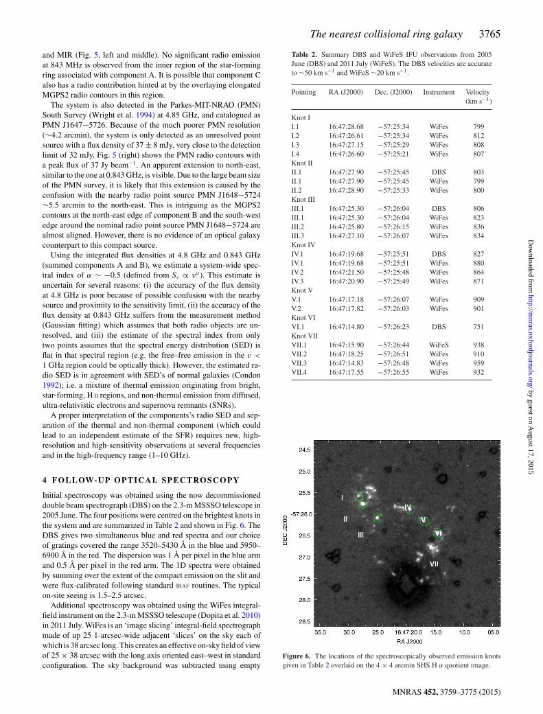
Initial spectroscopy was obtained using the now decommissioneddouble beam spectrograph (DBS) on the 2.3-m MSSSO telescope in2005 June. The four positions were centred on the brightest knots inthe system and are summarized in Table 2 and shown in Fig. 6. TheDBS gives two simultaneous blue and red spectra and our choiceof gratings covered the range 3520–5430 Å in the blue and 5950–6900 Å in the red. The dispersion was 1 Å per pixel in the blue armand 0.5 Å per pixel in the red arm. The 1D spectra were obtainedby summing over the extent of the compact emission on the slit andwere flux-calibrated following standard IRAF routines. The typicalon-site seeing is 1.5–2.5 arcsec.
Additional spectroscopy was obtained using the WiFes integral-field instrument on the 2.3-m MSSSO telescope (Dopita et al. 2010)in 2011 July. WiFes is an ‘image slicing’ integral-field spectrographmade of up 25 1-arcsec-wide adjacent ‘slices’ on the sky each ofwhich is 38 arcsec long. This creates an effective on-sky field of viewof 25 × 38 arcsec with the long axis oriented east–west in standardconfiguration. The sky background was subtracted using empty
Table 2. Summary DBS and WiFeS IFU observations from 2005June (DBS) and 2011 July (WiFeS). The DBS velocities are accurateto ∼50 km s−1 and WiFeS ∼20 km s−1.
Pointing RA (J2000) Dec. (J2000) Instrument Velocity(km s−1)
Knot II.1 16:47:28.68 −57:25:34 WiFes 799I.2 16:47:26.61 −57:25:34 WiFes 812I.3 16:47:27.15 −57:25:29 WiFes 808I.4 16:47:26.60 −57:25:21 WiFes 807Knot IIII.1 16:47:27.90 −57:25:45 DBS 803II.1 16:47:27.90 −57:25:45 WiFes 799II.2 16:47:28.90 −57:25:33 WiFes 800Knot IIIIII.1 16:47:25.30 −57:26:04 DBS 806III.1 16:47:25.30 −57:26:04 WiFes 823III.2 16:47:25.80 −57:26:15 WiFes 836III.3 16:47:27.10 −57:26:07 WiFes 834Knot IVIV.1 16:47:19.68 −57:25:51 DBS 827IV.1 16:47:19.68 −57:25:51 WiFes 880IV.2 16:47:21.50 −57:25:48 WiFes 864IV.3 16:47:20.90 −57:25:49 WiFes 871Knot VV.1 16:47:17.18 −57:26:07 WiFes 909V.2 16:47:17.82 −57:26:03 WiFes 901Knot VIVI.1 16:47:14.80 −57:26:23 DBS 751Knot VIIVII.1 16:47:15.90 −57:26:44 WiFeS 938VII.2 16:47:18.25 −57:26:51 WiFes 910VII.3 16:47:14.83 −57:26:48 WiFes 959VII.4 16:47:17.55 −57:26:55 WiFes 932
Figure 6. The locations of the spectroscopically observed emission knotsgiven in Table 2 overlaid on the 4 × 4 arcmin SHS H α quotient image.
MNRAS 452, 3759–3775 (2015)
by guest on August 17, 2015
http://mnras.oxfordjournals.org/
Dow
nloaded from
3766 Q. A. Parker et al.
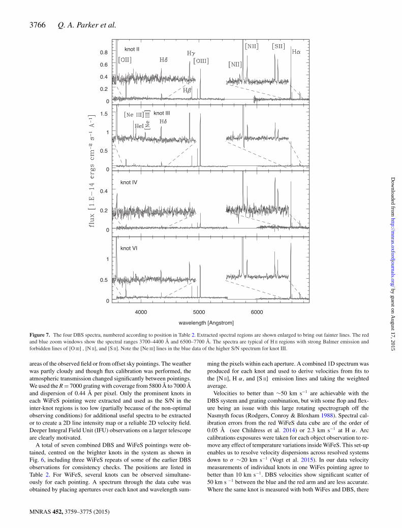
Figure 7. The four DBS spectra, numbered according to position in Table 2. Extracted spectral regions are shown enlarged to bring out fainter lines. The redand blue zoom windows show the spectral ranges 3700–4400 Å and 6500–7700 Å. The spectra are typical of H II regions with strong Balmer emission andforbidden lines of [O III] , [N II], and [S II]. Note the [Ne III] lines in the blue data of the higher S/N spectrum for knot III.
areas of the observed field or from offset sky pointings. The weatherwas partly cloudy and though flux calibration was performed, theatmospheric transmission changed significantly between pointings.We used the R = 7000 grating with coverage from 5800 Å to 7000 Åand dispersion of 0.44 Å per pixel. Only the prominent knots ineach WiFeS pointing were extracted and used as the S/N in theinter-knot regions is too low (partially because of the non-optimalobserving conditions) for additional useful spectra to be extractedor to create a 2D line intensity map or a reliable 2D velocity field.Deeper Integral Field Unit (IFU) observations on a larger telescopeare clearly motivated.
A total of seven combined DBS and WiFeS pointings were ob-tained, centred on the brighter knots in the system as shown inFig. 6, including three WiFeS repeats of some of the earlier DBSobservations for consistency checks. The positions are listed inTable 2. For WiFeS, several knots can be observed simultane-ously for each pointing. A spectrum through the data cube wasobtained by placing apertures over each knot and wavelength sum-
ming the pixels within each aperture. A combined 1D spectrum wasproduced for each knot and used to derive velocities from fits tothe [N II], H α, and [S II] emission lines and taking the weightedaverage.
Velocities to better than ∼50 km s−1 are achievable with theDBS system and grating combination, but with some flop and flex-ure being an issue with this large rotating spectrograph off theNasmyth focus (Rodgers, Conroy & Bloxham 1988). Spectral cal-ibration errors from the red WiFeS data cube are of the order of0.05 Å (see Childress et al. 2014) or 2.3 km s−1 at H α. Arccalibrations exposures were taken for each object observation to re-move any effect of temperature variations inside WiFeS. This set-upenables us to resolve velocity dispersions across resolved systemsdown to σ ∼20 km s−1 (Vogt et al. 2015). In our data velocitymeasurements of individual knots in one WiFes pointing agree tobetter than 10 km s−1. DBS velocities show significant scatter of50 km s −1 between the blue and the red arm and are less accurate.Where the same knot is measured with both WiFes and DBS, there
MNRAS 452, 3759–3775 (2015)
by guest on August 17, 2015
http://mnras.oxfordjournals.org/
Dow
nloaded from
The nearest collisional ring galaxy 3767
Table 3. SuperCOSMOS and SEXTRACTOR isophotal magnitude esti-mates for main system components. The asterisked I-band entry forcomponent A came from the IAM data from the SR/H α SuperCOS-MOS images and may be underestimated given the SEXTRACTOR value.SEXTRACTOR values are from Doyle et al. (2005).
Component Bj R1 R2 I Origin
A 13.1 – 13.3 12.8 SextractorA – 14.98 13.85 11.3* IAM (SuperCOS)B – 15.61 15.26 13.86 IAM (SuperCOS)C – 16.27 16.26 16.0 IAM (SuperCOS)
is acceptable agreement in two cases but the offset is fairly large(∼50 km s−1 in the third case (knot IV) and is at the upper errorlevel that might be expected. It is clear from Fig. 7 that the spectralcontinuum for Knot IV is lower than for the other spectra shown.
Fig. 7 presents the 1D blue and red emission line spectra from theDBS for knots II, III, IV and V. Extracted regions are shown enlargedto show the fainter lines. The spectra are typical of H II regions andexhibit the standard emission lines of [O II] 3727 Å, the Balmerseries (Hδ Hγ , Hβ) and [O III] in the blue region. In the red thereis H α and the weaker bracketing [N II] lines. The [S II] doublet isalso well detected and resolved providing an opportunity to estimateelectron densities. These are near the low-density limit (ne ≤100–200 cm−3) from measurements across four knots. For knot III,which is the highest surface brightness compact emission regionin the entire system, the higher S/N spectrum reveals [Ne III] linesat 3869 and 3968 Å rest wavelengths. There is no evidence forWolf–Rayet features in any of these H II region spectra.
5 A NA LY SIS
5.1 Optical photometry
Component A (the main ESO 179-13 galaxy) has optical photo-graphic photometry in the BJ, R, and I bands (Doyle et al, 2005),while Lee et al. (2011) give B 15. In the broad-band SuperCOS-MOS photographic data (Hambly et al. 2001a), the isophotal imageparameters for component A are blended with the bright star inthe BJ band, so no reliable magnitude is possible from the stan-dard image-analysis mode (IAM) processing. This led Doyle et al.(2005) to estimate individual SEXTRACTOR magnitudes for compo-nent A when constructing optical photometry for HIPASS galaxies.These were bootstrapped to the various SuperCOSMOS zero-pointsfor each band. However, the areal profile fitting and image deblend-ing techniques employed by the SuperCOSMOS IAM software(Hambly et al. 2001a) do enable component magnitude estimatesto be obtained. There are three R-band magnitudes available fromthe first and second epoch broad-band surveys and from the SRexposure taken as part of the H α survey. I-band SuperCOSMOSmagnitudes are also available. For isolated sources such magnitudesare accurate to ±0.1. These results are presented in Table 3. TheIAM results from components B and C are likely to be more reli-able than for component A whose I-band magnitude in particularseems grossly underestimated when compared to the independentSEXTRACTOR value from Doyle et al. (2005) and the 2MASS NIRphotometry for any sensible colour term. We estimate small colourterms of I − Ks ∼1.0 for component A and ∼1.4 for component B.
5.2 Infrared photometry
The available infrared photometry obtained is presented in Table 4with data gathered from various archives including Skrutskie et al.
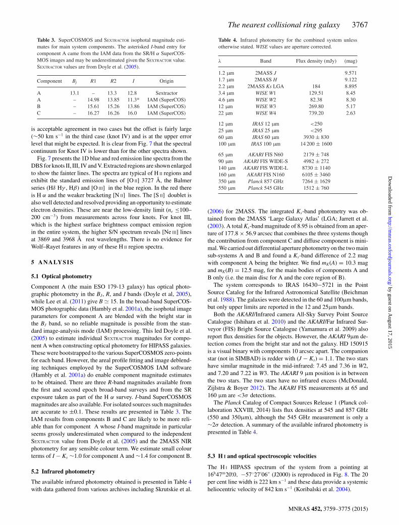
Table 4. Infrared photometry for the combined system unlessotherwise stated. WISE values are aperture corrected.
λ Band Flux density (mJy) (mag)
1.2 µm 2MASS J 9.5711.7 µm 2MASS H 9.1222.2 µm 2MASS Ks LGA 184 8.8953.4 µm WISE W1 129.51 8.454.6 µm WISE W2 82.38 8.3012 µm WISE W3 269.80 5.1722 µm WISE W4 739.20 2.63
12 µm IRAS 12 µm <25025 µm IRAS 25 µm <29560 µm IRAS 60 µm 3930 ± 830100 µm IRAS 100 µm 14 200 ± 1600
65 µm AKARI FIS N60 2179 ± 74890 µm AKARI FIS WIDE-S 4982 ± 272140 µm AKARI FIS WIDE-L 8730 ± 1140160 µm AKARI FIS N160 6105 ± 3460350 µm Planck 857 GHz 7264 ± 1629550 µm Planck 545 GHz 1512 ± 760
(2006) for 2MASS. The integrated Ks-band photometry was ob-tained from the 2MASS ‘Large Galaxy Atlas’ (LGA; Jarrett et al.(2003). A total Ks-band magnitude of 8.95 is obtained from an aper-ture of 177.8 × 56.9 arcsec that combines the three systems thoughthe contribution from component C and diffuse component is mini-mal. We carried out differential aperture photometry on the two mainsub-systems A and B and found a Ks-band difference of 2.2 magwith component A being the brighter. We find mK(A) = 10.3 magand mK(B) = 12.5 mag, for the main bodies of components A andB only (i.e. the main disc for A and the core region of B).
The system corresponds to IRAS 16430−5721 in the PointSource Catalog for the Infrared Astronomical Satellite (Beichmanet al. 1988). The galaxies were detected in the 60 and 100µm bands,but only upper limits are reported in the 12 and 25µm bands.
Both the AKARI/Infrared camera All-Sky Survey Point SourceCatalogue (Ishihara et al. 2010) and the AKARI/Far Infrared Sur-veyor (FIS) Bright Source Catalogue (Yamamura et al. 2009) alsoreport flux densities for the objects. However, the AKARI 9µm de-tection comes from the bright star and not the galaxy. HD 150915is a visual binary with components 10 arcsec apart. The companionstar (not in SIMBAD) is redder with (J − Ks) = 1.1. The two starshave similar magnitude in the mid-infrared: 7.45 and 7.36 in W2,and 7.20 and 7.22 in W3. The AKARI 9 µm position is in betweenthe two stars. The two stars have no infrared excess (McDonald,Zijlstra & Boyer 2012). The AKARI FIS measurements at 65 and160 µm are <3σ detections.
The Planck Catalog of Compact Sources Release 1 (Planck col-laboration XXVIII, 2014) lists flux densities at 545 and 857 GHz(550 and 350µm), although the 545 GHz measurement is only a∼2σ detection. A summary of the available infrared photometry ispresented in Table 4.
5.3 H I and optical spectroscopic velocities
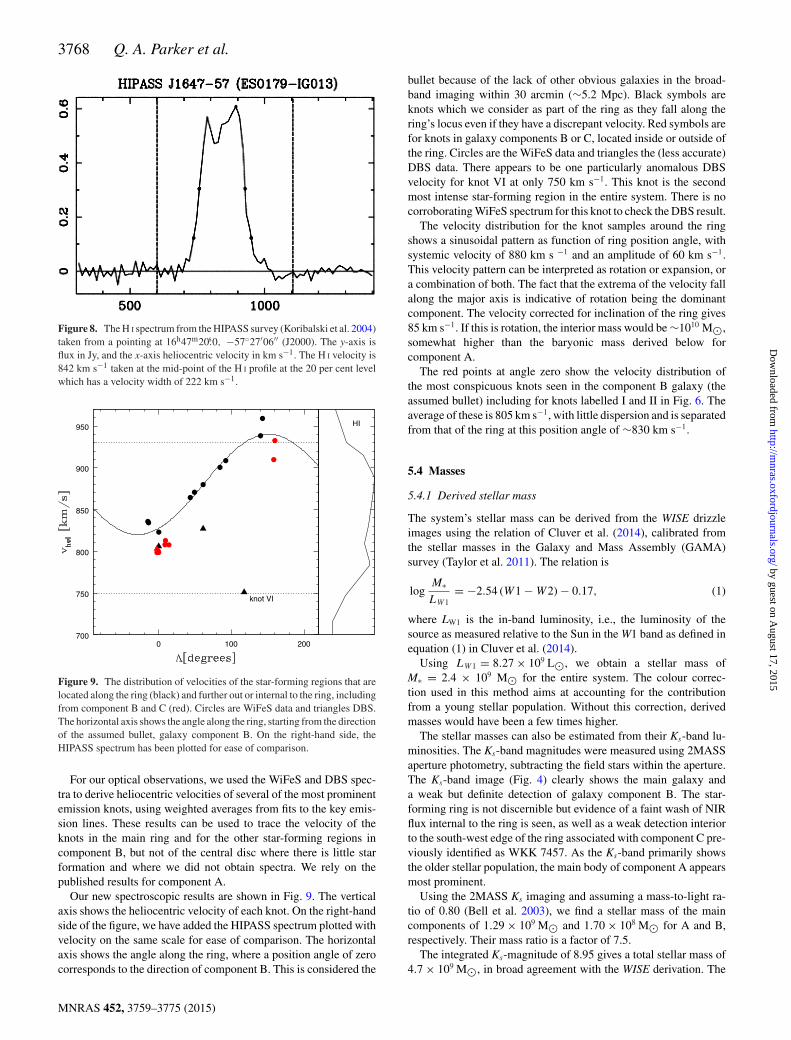
The H I HIPASS spectrum of the system from a pointing at16h47m20.s0, −57◦27′06′′ (J2000) is reproduced in Fig. 8. The 20per cent line width is 222 km s−1 and these data provide a systemicheliocentric velocity of 842 km s−1 (Koribalski et al. 2004).
MNRAS 452, 3759–3775 (2015)
by guest on August 17, 2015
http://mnras.oxfordjournals.org/
Dow
nloaded from
3768 Q. A. Parker et al.
Figure 8. The H I spectrum from the HIPASS survey (Koribalski et al. 2004)taken from a pointing at 16h47m20.s0, −57◦27′06′′ (J2000). The y-axis isflux in Jy, and the x-axis heliocentric velocity in km s−1. The H I velocity is842 km s−1 taken at the mid-point of the H I profile at the 20 per cent levelwhich has a velocity width of 222 km s−1.
Figure 9. The distribution of velocities of the star-forming regions that arelocated along the ring (black) and further out or internal to the ring, includingfrom component B and C (red). Circles are WiFeS data and triangles DBS.The horizontal axis shows the angle along the ring, starting from the directionof the assumed bullet, galaxy component B. On the right-hand side, theHIPASS spectrum has been plotted for ease of comparison.
For our optical observations, we used the WiFeS and DBS spec-tra to derive heliocentric velocities of several of the most prominentemission knots, using weighted averages from fits to the key emis-sion lines. These results can be used to trace the velocity of theknots in the main ring and for the other star-forming regions incomponent B, but not of the central disc where there is little starformation and where we did not obtain spectra. We rely on thepublished results for component A.
Our new spectroscopic results are shown in Fig. 9. The verticalaxis shows the heliocentric velocity of each knot. On the right-handside of the figure, we have added the HIPASS spectrum plotted withvelocity on the same scale for ease of comparison. The horizontalaxis shows the angle along the ring, where a position angle of zerocorresponds to the direction of component B. This is considered the
bullet because of the lack of other obvious galaxies in the broad-band imaging within 30 arcmin (∼5.2 Mpc). Black symbols areknots which we consider as part of the ring as they fall along thering’s locus even if they have a discrepant velocity. Red symbols arefor knots in galaxy components B or C, located inside or outside ofthe ring. Circles are the WiFeS data and triangles the (less accurate)DBS data. There appears to be one particularly anomalous DBSvelocity for knot VI at only 750 km s−1. This knot is the secondmost intense star-forming region in the entire system. There is nocorroborating WiFeS spectrum for this knot to check the DBS result.
The velocity distribution for the knot samples around the ringshows a sinusoidal pattern as function of ring position angle, withsystemic velocity of 880 km s −1 and an amplitude of 60 km s−1.This velocity pattern can be interpreted as rotation or expansion, ora combination of both. The fact that the extrema of the velocity fallalong the major axis is indicative of rotation being the dominantcomponent. The velocity corrected for inclination of the ring gives85 km s−1. If this is rotation, the interior mass would be ∼1010 M�,somewhat higher than the baryonic mass derived below forcomponent A.
The red points at angle zero show the velocity distribution ofthe most conspicuous knots seen in the component B galaxy (theassumed bullet) including for knots labelled I and II in Fig. 6. Theaverage of these is 805 km s−1, with little dispersion and is separatedfrom that of the ring at this position angle of ∼830 km s−1.
5.4 Masses
5.4.1 Derived stellar mass
The system’s stellar mass can be derived from the WISE drizzleimages using the relation of Cluver et al. (2014), calibrated fromthe stellar masses in the Galaxy and Mass Assembly (GAMA)survey (Taylor et al. 2011). The relation is
logM∗LW1
= −2.54 (W1 − W2) − 0.17, (1)
where LW1 is the in-band luminosity, i.e., the luminosity of thesource as measured relative to the Sun in the W1 band as defined inequation (1) in Cluver et al. (2014).
Using LW1 = 8.27 × 10⁹ L�, we obtain a stellar mass ofM∗ = 2.4 × 10⁹ M� for the entire system. The colour correc-tion used in this method aims at accounting for the contributionfrom a young stellar population. Without this correction, derivedmasses would have been a few times higher.
The stellar masses can also be estimated from their Ks-band lu-minosities. The Ks-band magnitudes were measured using 2MASSaperture photometry, subtracting the field stars within the aperture.The Ks-band image (Fig. 4) clearly shows the main galaxy anda weak but definite detection of galaxy component B. The star-forming ring is not discernible but evidence of a faint wash of NIRflux internal to the ring is seen, as well as a weak detection interiorto the south-west edge of the ring associated with component C pre-viously identified as WKK 7457. As the Ks-band primarily showsthe older stellar population, the main body of component A appearsmost prominent.
Using the 2MASS Ks imaging and assuming a mass-to-light ra-tio of 0.80 (Bell et al. 2003), we find a stellar mass of the maincomponents of 1.29 × 10⁹ M� and 1.70 × 10⁸ M� for A and B,respectively. Their mass ratio is a factor of 7.5.
The integrated Ks-magnitude of 8.95 gives a total stellar mass of4.7 × 109 M�, in broad agreement with the WISE derivation. The
MNRAS 452, 3759–3775 (2015)
by guest on August 17, 2015
http://mnras.oxfordjournals.org/
Dow
nloaded from
The nearest collisional ring galaxy 3769
mass-to-light ratio at Ks varies by a factor of 2 over a wide range ofstellar ages excluding the very youngest stars (Drory et al. 2004).The models of Henriques et al. (2011) show that the Ks-band can besignificantly enhanced by younger, more massive, asymptotic giantbranch stars, and include a component from red supergiants.
5.4.2 Gas and dust mass
The H I neutral hydrogen mass is reported by Koribalski et al. (2004)as MH I = 2 × 10⁹ M�. This is similar to the overall stellar mass ofthe entire system which is therefore gas rich. It is not clear where thebulk of the gas originates, but the large H I mass makes an originalassociation with component A more likely.
The mass in molecular gas is not known. CO data are required todetermine this directly. Stark et al. (2013), provide evaluations ofmolecular to neutral hydrogen (H2/H I) ratios from a broad sampleof field galaxies spanning early-to-late types, evolutionary stage andstellar masses of 107.2 to 1012 M�. Their sample is not statisticallyrepresentative because CO measurements for low-mass systemssuch as ours are lacking. It does seem that for a range in g − r of∼0.3, molecular to neutral gas ratios range from 1 to ∼10 per cent,so ∼109 M� in molecular hydrogen is possible.
We use two different methods to estimate dust masses usingavailable flux estimates. The AKARI 65, 90, 140, and 165 µm fluxdensities were measured using methods optimized for unresolvedsources (Yamamura et al. 2009). Since the system is larger thanthe AKARI beam, the AKARI measurements may miss some of theextended emission3 and could refer mainly to component A. Thiscould explain why the AKARI flux estimates are lower by a factor of2 compared to the equivalent IRAS values. In Table 4, we includedthe AKARI fluxes for completeness but only use the WISE, IRAS,and Planck data in this analysis.
The first method used fits the infrared SED with a blackbodyfunction multiplied by an emissivity function that scales as λ−β . Wethen used the resulting temperature T in the expression:
Mdust = fνD2
κνBν(T ), (2)
where fν is a flux density measured in a single waveband, D is thedistance to the source, κν is the wavelength-dependent opacity, andBν(T) is the blackbody function.
We perform fits to the data using β = 1.5, as found empiricallyby Boselli et al. (2012) using Herschel data, and β = 2, whichcorresponds to the theoretical emissivity function given by Li &Draine (2001) that is frequently used in dust mass calculations.We also use the κν based on values from Li & Draine (2001) tocalculate the dust mass corresponding to the modified blackbodyfits with β = 2. For other β values it is common to rescale κν
by (λ/λ0)−β , where λ0 is some reference wavelength where theemissivity is known. Though many authors select 250 µm as areference wavelength, it is unclear if this is appropriate, as thechoice is usually poorly justified. We only calculate dust masses forfits where β = 2, but still report the temperatures for both β = 1.5and β = 2. The dust masses from our fits are derived from theamplitudes of the best-fitting modified blackbody functions. Weuse a function for κν , where λ0 = 240 µm and κν(250 µm) =5.13 cm2 g−1.
3 Any contributions from the bright stars to the south are negligible, e.g. theSED for HD 150915 star drops by >3 orders of magnitude between 1 and10 µm.
Fits were performed to the 100, 350, and 550 µm data that tendto originate from the coldest and most massive dust componentheated by the diffuse interstellar radiation field. Emission at shorterwavelengths may come from a warmer thermal component (Bendoet al. 2006, 2012, 2015). The 100 µm emission may also originatein part or entirely from dust heated by star formation. We need thedata point to constrain the Wien side of the spectral energy SED,but we are also aware that the temperature may be overestimatedby our analysis and the dust mass underestimated.
We calculate the dust mass using the flux density at 350 µm,the longest wavelength at which we have a >3σ detection. Atshorter wavelengths, small uncertainties in the temperature willresult in relatively large uncertainties in the dust mass. We adoptκν(350 µm) = 2.43 g cm−2 for the opacity.
We obtain dust temperatures of 19 ± 2 K for fits with β = 2and 23 ± 3 K for β = 1.5. The slope of the 350–550µm data ismore consistent with a β = 2 emissivity function than the β = 1.5emissivity function found by Boselli et al. (2012), but given thelarge uncertainty in the 550µm data, it would be difficult to rule outthe possibility that β is smaller than or larger than 2. The dust massfor the fit corresponding to β = 2 is (1.1 ± 0.3) × 107 M�.
In the second method, we fit the model templates of Draine et al.(2007) to the data. These templates are calculated for several dif-ferent environments [the Milky Way, the LMC, and the Small Mag-ellanic Cloud (SMC)], different PAH mass fractions, and differentilluminating radiation fields. Draine et al. (2007) suggest fittingSED data using the following equation which we also adopt:
fν = A [(1 − γ )jν(UMIN) + γ jν(UMIN, UMAX)] . (3)
In this equation, jν(UMIN) is the template for dust heated by asingle radiation field UMIN and is equivalent to cirrus heated by adiffuse interstellar radiation field. The quantity jν(UMIN, UMAX) isthe template for dust heated by a range of illuminating radiationfields ranging from UMIN to UMAX, with the relation between theamount of dust dM heated by the given radiation field in the rangebetween U and U + dU given by the equation:
dM ∝ U−2 dU. (4)
This jν(UMIN, UMAX) effectively represents the fraction of dustheated by photodissociation regions (PDRs) in the fit, and the γ
term indicates the relative fraction of dust heated by the PDRs. TheA term is a constant that scales the sum of the jν functions (whichare in units of Jy cm2 sr −1 H-nucleon−1) to the flux density. It isrelated to the dust mass by
Mdust = Mdust
MgasmpD
2A, (5)
where Mdust/Mgas is the dust-to-gas ratio, mp is the mass of theproton, and D is the distance.
As this system shares many characteristics of dwarf galaxies andMagellanic systems (including the metallicity – see below), we onlyfit LMC and SMC templates to the data. We use all WISE, IRAS,and Planck data between 12 and 550µm in the fit.
We obtained best fits using templates based on the LMC2_05model from Draine et al. (2007). The resulting UMIN and UMAX
were 1.5 and 106 times the local interstellar radiation field. The best-fitting γ was 0.024 ± 0.017. This is consistent with the majorityor even all the dust mass being contained in a cirrus component.The resulting dust mass is (1.5 ± 0.3) × 107 M�, slightly higherthan that calculated using the single modified blackbody fit. This isexpected given that the Draine et al. (2007) models account for the
MNRAS 452, 3759–3775 (2015)
by guest on August 17, 2015
http://mnras.oxfordjournals.org/
Dow
nloaded from
3770 Q. A. Parker et al.
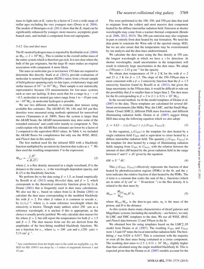
Table 5. Stellar, gas and dust masses, star formation rates, and specific star formation rates estimated for thefull system and, in so far as is known, for the individual components. Values for component A refer to theinner region (the disc), and for the core of component B. The SSFRs for A and B assume total stellar massesof 1.3 × 10⁹ and 1.7 × 10⁸ M�, respectively (refer to the text).
Parameter Full system Component A Component B Ring
M∗ (Ks) (M�) 4.7 × 10⁹ 1.3 × 10⁹ 1.7 × 10⁸ –M∗ (WISE) (M�) 2.4 × 10⁹ – – –MH I (M�) 2 × 10⁹ – – –Mdust (M�) 1.5 × 10⁷ – – –SFR (H α) (M� yr−1) 0.33 0.01 0.08 0.24SFR (WISE 12 µm) (M� yr−1) 0.15 – – –SFR (WISE 22 µm) (M� yr−1) 0.47 – – –SSFR (H α) (M� yr−1 M−1∗ ) 7.0 × 10⁻¹¹ 7.7 × 10⁻¹² 4.7 × 10⁻¹⁰ –
mass in warmer dust components and for the relative contributionsof various thermal components of dust to the SED.
The masses are summarized in Table 5. Individual stellar massesof the two systems are ∼3 times less than that of the total system, somuch of the stellar mass is located outside of the brighter regions.Deeper MIR images to find the detailed location of the remainder,either in a halo or in expelled streams, would be of interest.
The two galaxy components A and B are small systems. For com-parison, the stellar mass of the LMC is M = 2.7 × 10⁹ M�. Its W1flux is 2080 Jy (Melbourne & Boyer, 2013), which scaled to 10 Mpcgives 50 mJy, about three times fainter than Kathryn’s Wheel. Com-ponent A is similar to the LMC. Component B is comparable to theSMC, which has a stellar mass of 3.1 × 10⁸ M�.
The system contains more gas and dust than the LMC and SMC.The LMC H I mass is only 0.48 × 10⁹ M� (Staveley-Smith et al.2003), and the SMC has an H I mass of 5.6 × 10⁸ M� (Van derMarel, Kallivayalil & Besla 2009). While the stellar masses arebroadly comparable, the dust mass is three times higher and theneutral gas four times higher than that of the LMC and SMC com-bined. We do not know with certainty which of the two components(A or B) is the origin of the gas and dust emission. The gas-to-dustratio is ∼133, which excludes the unknown molecular mass and istherefore an upper limit. For comparison, a mean gas-to-dust ratioof 58.2 was found for 78 bright galaxies in the Herschel Virgo Clus-ter Survey (Davies et al. 2012). Based on their study, they suggestthat a factor of ∼2.9 can be used to convert atomic gas to total gas(i.e. H I + H 2) in their survey. The value of the gas-to-dust ratiofor the Milky Way is ∼143 (Draine et al. 2007), a similar valueto what we derive here. Interestingly, the ratio of the extent of thestar-forming regions within B to that of the ring around A is similarto the ratio of the galaxy stellar masses.
5.5 Star formation rates
SFR can be derived from different tracers (e.g. Kennicutt & Evans2012), mostly related to the UV photons produced by young massivestars. The H α luminosity and the MIR flux tracing heated dust areindependent tracers of the SFR.
5.5.1 SFR from the H α flux
The SFR from the integrated H α luminosity of the system is cal-culated following Kennicutt & Evans (2012), using the expression
logM∗
M� yr−1= log L(Hα) − 41.27. (6)
Our first estimate of the integrated H α flux (and luminosity) isderived from aperture photometry on all of the clearly identifiableknots in the CTIO continuum-subtracted H α image. These included43 knots in the ring, 8 knots in the core of component B, and 8 knotsin the region of the disc that defines component A. The resultingfluxes were converted to individual SFR for each knot.
Aperture photometry was also done on the full areas covered byeach of the main system components A, B, C, and the ring. Thisprovided a global integrated SFR as H α emission is distributedmore widely around the entire region and even at low levels alongthe main disc of component A. The results are listed in Table 5.For component B, we measured the main body, but excluded thefaint outer regions because of confusion with the ring to the south.Table 5 also lists the specific SFR (SSFR: the SFR divided by thestellar mass). For the disc system component A and for B, we usedthe stellar masses given in Table 5. No mass was derived for thering. For the full system we included all the stellar mass.
The conversion factor of flux units count−1 was derived from theindividual H II knots listed in Table 2, using a 7 arcsec aperture foreach. The H α flux for these knots was measured from the calibratedWiFeS IFU data. Poor weather during the WiFeS observations re-sulted in a factor of 2 spread in measured conversion factors. Re-moving the lower values left knot systems I, II, and IV. Averagingtheir conversion factors yields 1.2 ± 0.3 × 10⁻¹⁸ erg cm−2 s−1
per count for the CTIO image. The photometry counts were con-verted to flux units, and a total flux for all components of F(H α) =3.0 ± 0.6 × 10⁻¹² erg cm−2 s−1 was obtained.
Owing to possible problems with the flux calibration, an inde-pendent measurement would be useful. Unfortunately, the systemis just outside the footprint of the VST/OmegaCAM Photomet-ric H-Alpha Survey (VPHAS+) Survey (Drew et al. 2014), andwhile it is imaged by the calibrated low-resolution the Southern H-Alpha Sky Survey Atlas (SHASSA) survey (Gaustad et al. 2001),the proximity of HD 150915 precludes the measurement of an ac-curate integrated H α flux following the recipe of Frew, Bojicic& Parker (2013). However, the SHS (Parker et al. 2005) offers analternative approach to obtaining the integrated H α flux of thesystem, in order to compare with our CTIO estimate. The SHSwas absolutely calibrated by Frew et al. (2014a), who showed fluxmeasurements to 20–50 per cent accuracy were feasible for non-saturated diffuse emission regions. Using the methods discussedthere, and correcting for reduced transmission due to the systemicvelocity, we determine an integrated H α flux of 1.1 ± 0.5 ×10⁻¹² erg cm−2 s−1 for component B through an aperture of90 arcsec; a correction for [N II] contamination is unnecessarybased on the high excitation and low metallicity of the system’s
MNRAS 452, 3759–3775 (2015)
by guest on August 17, 2015
http://mnras.oxfordjournals.org/
Dow
nloaded from
The nearest collisional ring galaxy 3771
H II regions. This agrees with an equivalent CTIO measurement towithin the uncertainties, so we average the results to get a totalflux for component B. Unfortunately the proximity of the brightstar precludes an accurate flux measurement from the SHS for thestar-forming ring. An approximate lower limit, based on a simplecurve-of-growth analysis of several apertures is F(H α) = ∼1 ×10⁻¹² erg cm−2 s−1, also in agreement with the CTIO measure-ment. The total H α flux for the system, now using the weightedaverage of the independent CTIO and SHS calibrations, is 2.9 ± 0.3× 10⁻¹² erg cm−2 s−1, adopted hereafter.
The systemic flux, now corrected for a reddening E(B − V) =0.24 mag, and applying a Howarth (1983) reddening law, isF0(H α) = 5.1 × 10⁻¹² erg cm−2 s−1. This leads to a total lu-minosity, L(Hα) = 6.1 × 1040 erg s−1, and a total ionizing flux,Q = 4.4 × 1052 photons s−1, for a distance of 10 Mpc. The inte-grated SFR was then found to be 0.33 ± 0.09 M� yr−1 followingequation (6). This SFR is about 60 per cent higher than that of theLMC, adopting the H α luminosity for the LMC from Kennicuttet al. (1995). Our estimate may be an underestimate as we havenot corrected for any local extinction, though the extinction derivedfrom the mean Balmer decrement of the brightest H II regions fromour spectra is consistent with the Schlafly & Finkbeiner (2011) ex-tinction, indicating that the internal reddening is, in at least the mostluminous H II regions, minimal. There may also be photon leakagefrom the larger H II regions in the system as noted by Relano et al.(2012), which might help to explain the difference between theSFRs derived from H α and 22 µm WISE flux (see below).
We note that the most luminous H II region complex in ESO 179-13 is centred on knot VII, with L(Hα) 5 × 1039 erg s−1. Thisluminosity is comparable to supergiant H II regions like 30 Doradusin the LMC and NGC 604 in M 33 (Kennicutt 1984). Knot VII iswithin component C which contains old stars as it is detected inthe 2MASS imagery as a separate object. It also lies interior to thefitted ring and has a different velocity distribution to the componentsalong the ring, exhibiting the largest velocities across the system.We still consider it likely to be a separate star-forming dwarf galaxybut further observations are required to establish this clearly and tostudy the relationship between components A and C.
5.5.2 SFR from the MIR flux
The warm dust continuum is best traced by the 22 µm WISE flux.Cluver et al. (2014) have calibrated the relation of this flux againstH α-derived SFRs (corrected for extinction) from the GAMA Sur-vey (Gunawardhana et al. 2013) and find
logM∗
M� yr−1= 0.82 log νL(22 µm[L�]) − 7.3. (7)
This yields an integrated SFR of 0.47 M� yr−1 for ESO 179-13,somewhat higher than that derived from the de-reddened H α flux.In contrast, the 12 µm emission (Cluver et al. 2014), calibratedin the same way, corresponds to a lower SFR of 0.15 M� yr−1.The lower mass measured in the 12 µm band may be because thisband detects significant PAH emission. This is relatively weak inlow metallicity environments (e.g. Engelbracht et al. 2005, 2008),so emission from bands that contain PAH emission and the SFRsbased on these bands may be underestimated. All in all, the variousestimates are in reasonable agreement, and we conclude that theintegrated SFR is approximately 0.2–0.5 M� yr−1.
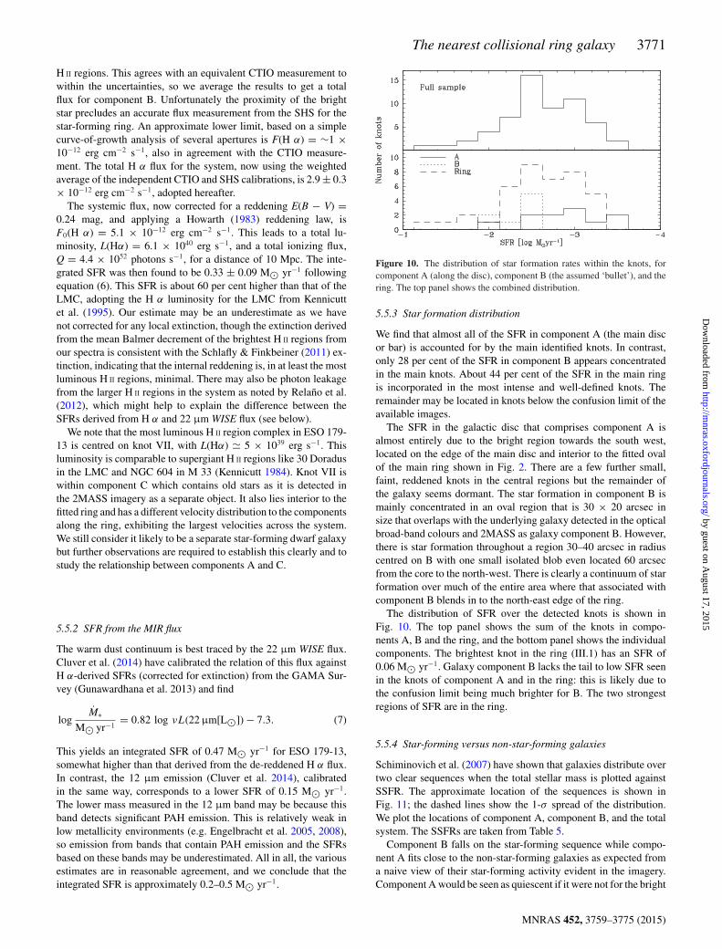
Figure 10. The distribution of star formation rates within the knots, forcomponent A (along the disc), component B (the assumed ‘bullet’), and thering. The top panel shows the combined distribution.
5.5.3 Star formation distribution
We find that almost all of the SFR in component A (the main discor bar) is accounted for by the main identified knots. In contrast,only 28 per cent of the SFR in component B appears concentratedin the main knots. About 44 per cent of the SFR in the main ringis incorporated in the most intense and well-defined knots. Theremainder may be located in knots below the confusion limit of theavailable images.
The SFR in the galactic disc that comprises component A isalmost entirely due to the bright region towards the south west,located on the edge of the main disc and interior to the fitted ovalof the main ring shown in Fig. 2. There are a few further small,faint, reddened knots in the central regions but the remainder ofthe galaxy seems dormant. The star formation in component B ismainly concentrated in an oval region that is 30 × 20 arcsec insize that overlaps with the underlying galaxy detected in the opticalbroad-band colours and 2MASS as galaxy component B. However,there is star formation throughout a region 30–40 arcsec in radiuscentred on B with one small isolated blob even located 60 arcsecfrom the core to the north-west. There is clearly a continuum of starformation over much of the entire area where that associated withcomponent B blends in to the north-east edge of the ring.
The distribution of SFR over the detected knots is shown inFig. 10. The top panel shows the sum of the knots in compo-nents A, B and the ring, and the bottom panel shows the individualcomponents. The brightest knot in the ring (III.1) has an SFR of0.06 M� yr−1. Galaxy component B lacks the tail to low SFR seenin the knots of component A and in the ring: this is likely due tothe confusion limit being much brighter for B. The two strongestregions of SFR are in the ring.
5.5.4 Star-forming versus non-star-forming galaxies
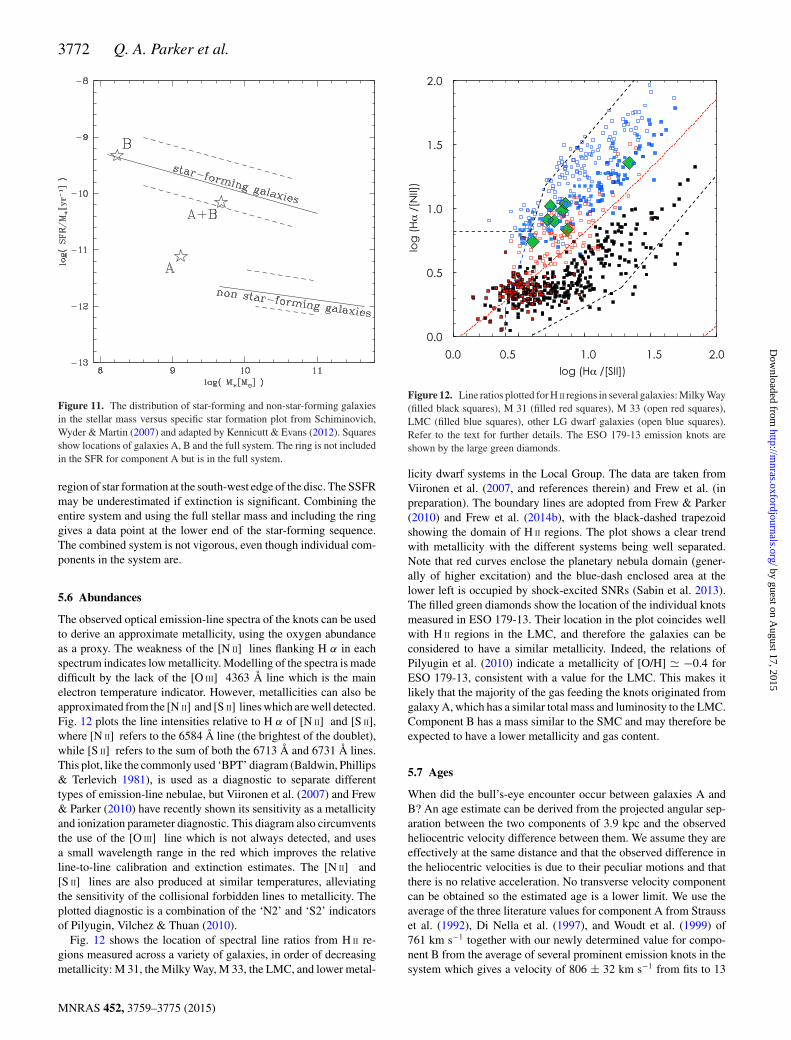
Schiminovich et al. (2007) have shown that galaxies distribute overtwo clear sequences when the total stellar mass is plotted againstSSFR. The approximate location of the sequences is shown inFig. 11; the dashed lines show the 1-σ spread of the distribution.We plot the locations of component A, component B, and the totalsystem. The SSFRs are taken from Table 5.
Component B falls on the star-forming sequence while compo-nent A fits close to the non-star-forming galaxies as expected froma naive view of their star-forming activity evident in the imagery.Component A would be seen as quiescent if it were not for the bright
MNRAS 452, 3759–3775 (2015)
by guest on August 17, 2015
http://mnras.oxfordjournals.org/
Dow
nloaded from
3772 Q. A. Parker et al.
Figure 11. The distribution of star-forming and non-star-forming galaxiesin the stellar mass versus specific star formation plot from Schiminovich,Wyder & Martin (2007) and adapted by Kennicutt & Evans (2012). Squaresshow locations of galaxies A, B and the full system. The ring is not includedin the SFR for component A but is in the full system.
region of star formation at the south-west edge of the disc. The SSFRmay be underestimated if extinction is significant. Combining theentire system and using the full stellar mass and including the ringgives a data point at the lower end of the star-forming sequence.The combined system is not vigorous, even though individual com-ponents in the system are.
5.6 Abundances
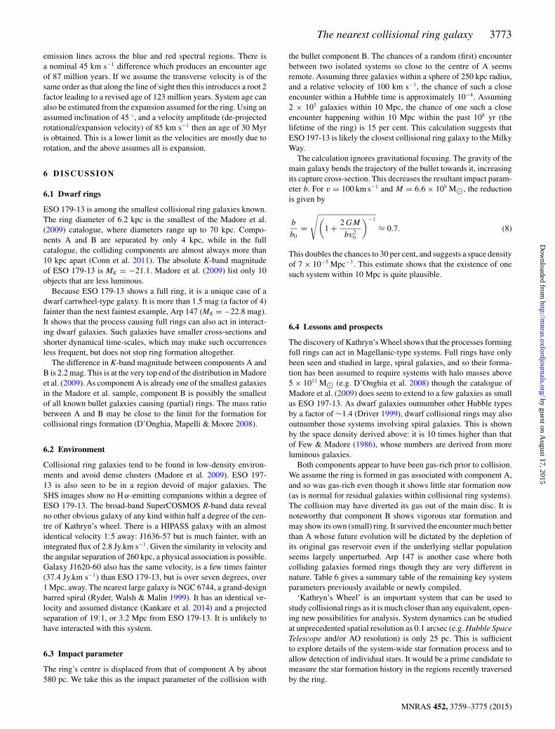
The observed optical emission-line spectra of the knots can be usedto derive an approximate metallicity, using the oxygen abundanceas a proxy. The weakness of the [N II] lines flanking H α in eachspectrum indicates low metallicity. Modelling of the spectra is madedifficult by the lack of the [O III] 4363 Å line which is the mainelectron temperature indicator. However, metallicities can also beapproximated from the [N II] and [S II] lines which are well detected.Fig. 12 plots the line intensities relative to H α of [N II] and [S II],where [N II] refers to the 6584 Å line (the brightest of the doublet),while [S II] refers to the sum of both the 6713 Å and 6731 Å lines.This plot, like the commonly used ‘BPT’ diagram (Baldwin, Phillips& Terlevich 1981), is used as a diagnostic to separate differenttypes of emission-line nebulae, but Viironen et al. (2007) and Frew& Parker (2010) have recently shown its sensitivity as a metallicityand ionization parameter diagnostic. This diagram also circumventsthe use of the [O III] line which is not always detected, and usesa small wavelength range in the red which improves the relativeline-to-line calibration and extinction estimates. The [N II] and[S II] lines are also produced at similar temperatures, alleviatingthe sensitivity of the collisional forbidden lines to metallicity. Theplotted diagnostic is a combination of the ‘N2’ and ‘S2’ indicatorsof Pilyugin, Vilchez & Thuan (2010).
Fig. 12 shows the location of spectral line ratios from H II re-gions measured across a variety of galaxies, in order of decreasingmetallicity: M 31, the Milky Way, M 33, the LMC, and lower metal-
Figure 12. Line ratios plotted for H II regions in several galaxies: Milky Way(filled black squares), M 31 (filled red squares), M 33 (open red squares),LMC (filled blue squares), other LG dwarf galaxies (open blue squares).Refer to the text for further details. The ESO 179-13 emission knots areshown by the large green diamonds.
licity dwarf systems in the Local Group. The data are taken fromViironen et al. (2007, and references therein) and Frew et al. (inpreparation). The boundary lines are adopted from Frew & Parker(2010) and Frew et al. (2014b), with the black-dashed trapezoidshowing the domain of H II regions. The plot shows a clear trendwith metallicity with the different systems being well separated.Note that red curves enclose the planetary nebula domain (gener-ally of higher excitation) and the blue-dash enclosed area at thelower left is occupied by shock-excited SNRs (Sabin et al. 2013).The filled green diamonds show the location of the individual knotsmeasured in ESO 179-13. Their location in the plot coincides wellwith H II regions in the LMC, and therefore the galaxies can beconsidered to have a similar metallicity. Indeed, the relations ofPilyugin et al. (2010) indicate a metallicity of [O/H] −0.4 forESO 179-13, consistent with a value for the LMC. This makes itlikely that the majority of the gas feeding the knots originated fromgalaxy A, which has a similar total mass and luminosity to the LMC.Component B has a mass similar to the SMC and may therefore beexpected to have a lower metallicity and gas content.
5.7 Ages
When did the bull’s-eye encounter occur between galaxies A andB? An age estimate can be derived from the projected angular sep-aration between the two components of 3.9 kpc and the observedheliocentric velocity difference between them. We assume they areeffectively at the same distance and that the observed difference inthe heliocentric velocities is due to their peculiar motions and thatthere is no relative acceleration. No transverse velocity componentcan be obtained so the estimated age is a lower limit. We use theaverage of the three literature values for component A from Strausset al. (1992), Di Nella et al. (1997), and Woudt et al. (1999) of761 km s−1 together with our newly determined value for compo-nent B from the average of several prominent emission knots in thesystem which gives a velocity of 806 ± 32 km s−1 from fits to 13
MNRAS 452, 3759–3775 (2015)
by guest on August 17, 2015
http://mnras.oxfordjournals.org/
Dow
nloaded from
The nearest collisional ring galaxy 3773
emission lines across the blue and red spectral regions. There isa nominal 45 km s−1 difference which produces an encounter ageof 87 million years. If we assume the transverse velocity is of thesame order as that along the line of sight then this introduces a root 2factor leading to a revised age of 123 million years. System age canalso be estimated from the expansion assumed for the ring. Using anassumed inclination of 45 ◦, and a velocity amplitude (de-projectedrotational/expansion velocity) of 85 km s−1 then an age of 30 Myris obtained. This is a lower limit as the velocities are mostly due torotation, and the above assumes all is expansion.
6 D ISCUSSION
6.1 Dwarf rings
ESO 179-13 is among the smallest collisional ring galaxies known.The ring diameter of 6.2 kpc is the smallest of the Madore et al.(2009) catalogue, where diameters range up to 70 kpc. Compo-nents A and B are separated by only 4 kpc, while in the fullcatalogue, the colliding components are almost always more than10 kpc apart (Conn et al. 2011). The absolute K-band magnitudeof ESO 179-13 is MK = −21.1. Madore et al. (2009) list only 10objects that are less luminous.
Because ESO 179-13 shows a full ring, it is a unique case of adwarf cartwheel-type galaxy. It is more than 1.5 mag (a factor of 4)fainter than the next faintest example, Arp 147 (MK = −22.8 mag).It shows that the process causing full rings can also act in interact-ing dwarf galaxies. Such galaxies have smaller cross-sections andshorter dynamical time-scales, which may make such occurrencesless frequent, but does not stop ring formation altogether.
The difference in K-band magnitude between components A andB is 2.2 mag. This is at the very top end of the distribution in Madoreet al. (2009). As component A is already one of the smallest galaxiesin the Madore et al. sample, component B is possibly the smallestof all known bullet galaxies causing (partial) rings. The mass ratiobetween A and B may be close to the limit for the formation forcollisional rings formation (D’Onghia, Mapelli & Moore 2008).
6.2 Environment
Collisional ring galaxies tend to be found in low-density environ-ments and avoid dense clusters (Madore et al. 2009). ESO 197-13 is also seen to be in a region devoid of major galaxies. TheSHS images show no H α-emitting companions within a degree ofESO 179-13. The broad-band SuperCOSMOS R-band data revealno other obvious galaxy of any kind within half a degree of the cen-tre of Kathryn’s wheel. There is a HIPASS galaxy with an almostidentical velocity 1.◦5 away: J1636-57 but is much fainter, with anintegrated flux of 2.8 Jy.km s−1. Given the similarity in velocity andthe angular separation of 260 kpc, a physical association is possible.Galaxy J1620-60 also has the same velocity, is a few times fainter(37.4 Jy.km s−1) than ESO 179-13, but is over seven degrees, over1 Mpc, away. The nearest large galaxy is NGC 6744, a grand-designbarred spiral (Ryder, Walsh & Malin 1999). It has an identical ve-locity and assumed distance (Kankare et al. 2014) and a projectedseparation of 19.◦1, or 3.2 Mpc from ESO 179-13. It is unlikely tohave interacted with this system.
6.3 Impact parameter
The ring’s centre is displaced from that of component A by about580 pc. We take this as the impact parameter of the collision with
the bullet component B. The chances of a random (first) encounterbetween two isolated systems so close to the centre of A seemsremote. Assuming three galaxies within a sphere of 250 kpc radius,and a relative velocity of 100 km s−1, the chance of such a closeencounter within a Hubble time is approximately 10−4. Assuming2 × 105 galaxies within 10 Mpc, the chance of one such a closeencounter happening within 10 Mpc within the past 108 yr (thelifetime of the ring) is 15 per cent. This calculation suggests thatESO 197-13 is likely the closest collisional ring galaxy to the MilkyWay.
The calculation ignores gravitational focusing. The gravity of themain galaxy bends the trajectory of the bullet towards it, increasingits capture cross-section. This decreases the resultant impact param-eter b. For v = 100 km s−1 and M = 6.6 × 10⁹ M�, the reductionis given by
b
b0=
√(1 + 2 GM
bv20
)−1
≈ 0.7. (8)
This doubles the chances to 30 per cent, and suggests a space densityof 7 × 10⁻⁵ Mpc−3. This estimate shows that the existence of onesuch system within 10 Mpc is quite plausible.
6.4 Lessons and prospects
The discovery of Kathryn’s Wheel shows that the processes formingfull rings can act in Magellanic-type systems. Full rings have onlybeen seen and studied in large, spiral galaxies, and so their forma-tion has been assumed to require systems with halo masses above5 × 1011 M� (e.g. D’Onghia et al. 2008) though the catalogue ofMadore et al. (2009) does seem to extend to a few galaxies as smallas ESO 197-13. As dwarf galaxies outnumber other Hubble typesby a factor of ∼1.4 (Driver 1999), dwarf collisional rings may alsooutnumber those systems involving spiral galaxies. This is shownby the space density derived above: it is 10 times higher than thatof Few & Madore (1986), whose numbers are derived from moreluminous galaxies.
Both components appear to have been gas-rich prior to collision.We assume the ring is formed in gas associated with component A,and so was gas-rich even though it shows little star formation now(as is normal for residual galaxies within collisional ring systems).The collision may have diverted its gas out of the main disc. It isnoteworthy that component B shows vigorous star formation andmay show its own (small) ring. It survived the encounter much betterthan A whose future evolution will be dictated by the depletion ofits original gas reservoir even if the underlying stellar populationseems largely unperturbed. Arp 147 is another case where bothcolliding galaxies formed rings though they are very different innature. Table 6 gives a summary table of the remaining key systemparameters previously available or newly compiled.
‘Kathryn’s Wheel’ is an important system that can be used tostudy collisional rings as it is much closer than any equivalent, open-ing new possibilities for analysis. System dynamics can be studiedat unprecedented spatial resolution as 0.1 arcsec (e.g. Hubble SpaceTelescope and/or AO resolution) is only 25 pc. This is sufficientto explore details of the system-wide star formation process and toallow detection of individual stars. It would be a prime candidate tomeasure the star formation history in the regions recently traversedby the ring.
MNRAS 452, 3759–3775 (2015)
by guest on August 17, 2015
http://mnras.oxfordjournals.org/
Dow
nloaded from
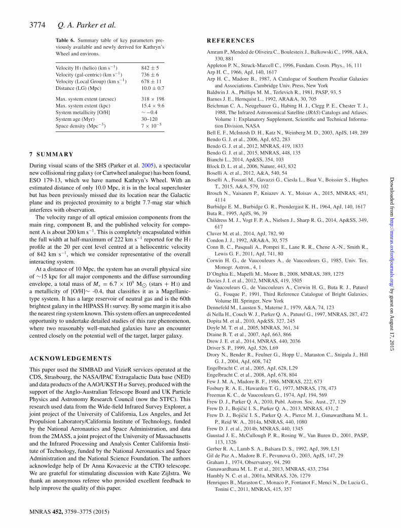
3774 Q. A. Parker et al.
Table 6. Summary table of key parameters pre-viously available and newly derived for Kathryn’sWheel and environs.
Velocity H I (helio) (km s−1) 842 ± 5Velocity (gal-centric) (km s−1) 736 ± 6Velocity (Local Group) (km s−1) 678 ± 11Distance (LG) (Mpc) 10.0 ± 0.7
Max. system extent (arcsec) 318 × 198Max. system extent (kpc) 15.4 × 9.6System metallicity [O/H] ∼−0.4System age (Myr) 30–120Space density (Mpc−3) 7 × 10⁻⁵
7 SU M M A RY
During visual scans of the SHS (Parker et al. 2005), a spectacularnew collisional ring galaxy (or Cartwheel analogue) has been found,ESO 179-13, which we have named Kathryn’s Wheel. With anestimated distance of only 10.0 Mpc, it is in the local superclusterbut has been previously missed due its location near the Galacticplane and its projected proximity to a bright 7.7-mag star whichinterferes with observation.
The velocity range of all optical emission components from themain ring, component B, and the published velocity for compo-nent A is about 200 km s−1. This is completely encapsulated withinthe full width at half-maximum of 222 km s−1 reported for the H I
profile at the 20 per cent level centred at a heliocentric velocityof 842 km s−1, which we consider representative of the overallinteracting system.
At a distance of 10 Mpc, the system has an overall physical sizeof ∼15 kpc for all major components and the diffuse surroundingenvelope, a total mass of M∗ = 6.7 × 10⁹ M� (stars + H I) anda metallicity of [O/H]∼ -0.4, that classifies it as a Magellanic-type system. It has a large reservoir of neutral gas and is the 60thbrightest galaxy in the HIPASS H I survey. By some margin it is alsothe nearest ring system known. This system offers an unprecedentedopportunity to undertake detailed studies of this rare phenomenon,where two reasonably well-matched galaxies have an encountercentred closely on the potential well of the target, larger galaxy.
AC K N OW L E D G E M E N T S
This paper used the SIMBAD and VizieR services operated at theCDS, Strasbourg, the NASA/IPAC Extragalactic Data base (NED)and data products of the AAO/UKST H α Survey, produced with thesupport of the Anglo-Australian Telescope Board and UK ParticlePhysics and Astronomy Research Council (now the STFC). Thisresearch used data from the Wide-field Infrared Survey Explorer, ajoint project of the University of California, Los Angeles, and JetPropulsion Laboratory/California Institute of Technology, fundedby the National Aeronautics and Space Administration, and datafrom the 2MASS, a joint project of the University of Massachusettsand the Infrared Processing and Analysis Center California Insti-tute of Technology, funded by the National Aeronautics and SpaceAdministration and the National Science Foundation. The authorsacknowledge help of Dr Anna Kovacevic at the CTIO telescope.We are grateful for stimulating discussion with Kate Zijlstra. Wethank an anonymous referee who provided excellent feedback tohelp improve the quality of this paper.
R E F E R E N C E S
Amram P., Mended de Oliveira C., Boulesteix J., Balkowski C., 1998, A&A,330, 881
Appleton P. N., Struck-Marcell C., 1996, Fundam. Cosm. Phys., 16, 111Arp H. C., 1966, ApJ, 140, 1617Arp H. C., Madore B., 1987, A Catalogue of Southern Peculiar Galaxies
and Associations. Cambridge Univ. Press, New YorkBaldwin J. A., Phillips M. M., Terlevich R., 1981, PASP, 93, 5Barnes J. E., Hernquist L., 1992, ARA&A, 30, 705Beichman C. A., Neugebauer G., Habing H. J., Clegg P. E., Chester T. J.,
1988, The Infrared Astronomical Satellite (IRAS) Catalogs and Atlases.Volume 1: Explanatory Supplement, Scientific and Technical Informa-tion Division, NASA
Bell E. F., McIntosh D. H., Katz N., Weinberg M. D., 2003, ApJS, 149, 289Bendo G. J. et al., 2006, ApJ, 652, 283Bendo G. J. et al., 2012, MNRAS, 419, 1833Bendo G. J. et al., 2015, MNRAS, 448, 135Bianchi L., 2014, Ap&SS, 354, 103Block D. L. et al., 2006, Nature, 443, 832Boselli A. et al., 2012, A&A, 540, 54Boselli A., Fossati M., Gavazzi G., Ciesla L., Buat V., Boissier S., Hughes
T., 2015, A&A, 579, 102Brosch N., Vaisanen P., Kniazev A. Y., Moisav A., 2015, MNRAS, 451,
4114Burbidge E. M., Burbidge G. R., Prendergast K. H., 1964, ApJ, 140, 1617Buta R., 1995, ApJS, 96, 39Childress M. J., Vogt F. P. A., Nielsen J., Sharp R. G., 2014, Ap&SS, 349,
617Cluver M. et al., 2014, ApJ, 782, 90Condon J. J., 1992, ARA&A, 30, 575Conn B. C., Pasquali A., Pompei E., Lane R. R., Chene A.-N., Smith R.,
Lewis G. F., 2011, ApJ, 741, 80Corwin H. G., de Vaucouleurs A., de Vaucouleurs G., 1985, Univ. Tex.
Monogr. Astron., 4, 1D’Onghia E., Mapelli M., Moore B., 2008, MNRAS, 389, 1275Davies J. I. et al., 2012, MNRAS, 419, 3505de Vaucouleurs G., de Vaucouleurs A., Corwin H. G., Buta R. J., Paturel
G., Fouque P., 1991, Third Reference Catalogue of Bright Galaxies,Volume III. Springer, New York
Dennefeld M., Lausten S., Materne J., 1979, A&A, 74, 123di Nella H., Couch W. J., Parker Q. A., Paturel G., 1997, MNRAS, 287, 472Dopita M. et al., 2010, Ap&SS, 327, 245Doyle M. T. et al., 2005, MNRAS, 361, 34Draine B. T. et al., 2007, ApJ, 663, 866Drew J. E. et al., 2014, MNRAS, 440, 2036Driver S. P., 1999, ApJ, 526, L69Drory N., Bender R., Feulner G., Hopp U., Maraston C., Snigula J., Hill
G. J., 2004, ApJ, 608, 742Engelbracht C. et al., 2005, ApJ, 628, L29Engelbracht C. et al., 2008, ApJ, 678, 804Few J. M. A., Madore B. F., 1986, MNRAS, 222, 673Fosbury R. A. E., Hawarden T. G., 1977, MNRAS, 178, 473Freeman K. C., de Vaucouleurs G., 1974, ApJ, 194, 569Frew D. J., Parker Q. A., 2010, Publ. Astron. Soc. Aust., 27, 129Frew D. J., Bojicic I. S., Parker Q. A., 2013, MNRAS, 431, 2Frew D. J., Bojicic I. S., Parker Q. A., Pierce M. J., Gunawardhana M. L.
P., Reid W. A., 2014a, MNRAS, 440, 1080Frew D. J. et al., 2014b, MNRAS, 440, 1345Gaustad J. E., McCullough P. R., Rosing W., Van Buren D., 2001, PASP,
113, 1326Gerber R. A., Lamb S. A., Balsara D. S., 1992, ApJ, 399, L51Gil de Paz A., Madore B. F., Pevunova O., 2003, ApJS, 147, 29Graham J., 1974, Observatory, 94, 290Gunawardhana M. L. P. et al., 2013, MNRAS, 433, 2764Hambly N. C. et al., 2001a, MNRAS, 326, 1279Henriques B., Maraston C., Monaco P., Fontanot F., Menci N., De Lucia G.,
Tonini C., 2011, MNRAS, 415, 357
MNRAS 452, 3759–3775 (2015)
by guest on August 17, 2015
http://mnras.oxfordjournals.org/
Dow
nloaded from
The nearest collisional ring galaxy 3775
Higdon J. L., Higdon S. J. U., Rand R. J., 2011, ApJ, 739, 97Hinshaw G. et al., 2013, ApJS, 208, 19Howarth I., 1983, MNRAS, 203, 301Ishihara D. et al., 2010, A&A, 514, 1James P. A. et al., 2004, A&A, 414, 23Jarrett T. H., Chester T., Cutri R., Schneider S. E., Huchra J. P., 2003, AJ,
125, 525Jarrett T. H. et al., 2012, AJ, 144, 68Kankare E. et al., 2014, A&A, 572, A75Kennicutt R. C., 1984, ApJ, 287, 116Kennicutt R. C., Evans N. J., 2012, ARA&A, 50, 531Kennicutt R. C., Bresolin F., Bomans D. J., Bothun G. D., Thompson I. B.,
1995, AJ, 109, 594Kennicutt R. C., Lee J. C., Funes S. J., Jose G., Sakai S., Akiyama S., 2008,
ApJS, 178, 247Koribalski B. S. et al., 2004, AJ, 1, 16Lauberts A., 1982, ESO/Uppsala Survey of the ESO(B) Atlas. European
Southern Observatory, GarchingLaustsen S., Madsen C., West R. M., 1987, Exploring the Southern Sky.
European Southern Observatory, GarchingLee J. C. et al., 2011, ApJS, 192, 33Li A., Draine B. T., 2001, ApJ, 554, 778Lindsay E. M., Shapley H., 1960, Observatory, 80, 223Longmore A. J. et al., 1982, MNRAS, 200, 325Madore B. F., Nelson E., Petrillo K., 2009, ApJS, 181, 572Marston A. P., Appleton P. N., 1995, AJ, 109, 1002Masci F., 2013, Astrophysics Source Code Library, record ascl:1302.010Masci F. J., Fowler J. W., 2009, in David A. B., Daniel D., Patrick D., ASP
Conf. Ser. Vol. 411, Astronomical Data Analysis Software and SystemsXVIII. Astron. Soc. Pac., San Francisco, p. 67
McDonald I., Zijlstra A. A., Boyer M. L., 2012, MNRAS, 427, 343Melbourne J., Boyer M. L., 2013, ApJ, 764, 30Meyer M. J. et al., 2004, MNRAS, 350, 1195Murphy T., Mauch T., Green A., Hunstead R. W., Piestrzynska B., Kels
A. P., Sztajer P., 2007, MNRAS, 382, 382Parker Q. A., Bland-Hawthorn J., 1998, Publ. Astron. Soc. Aust., 15, 33Parker Q. A. et al., 2005, MNRAS, 362, 689Parker Q. A. et al., 2006, MNRAS, 372, 79Pilyugin L. S., Vilchez J. M., Thuan T. X., 2010, ApJ 720, 1738Planck Collaboration XXVIII, 2014, A&A, 571, 28Relano M., Kennicutt R. C., Eldridge J. J., Lee J. C., Verley S., 2012,
MNRAS, 423, 2933Rodgers A. W., Conroy P., Bloxham G., 1988, PASP, 100, 626
Romano R., Mayya Y. D., Vorobyov E. I., 2008, AJ, 136, 1259Ryder S. D., Walsh W., Malin D., 1999, Publ. Astron. Soc. Aust., 16, 84Sabin L. et al., 2013, MNRAS, 431, 279Schiminovich D., Wyder T. K., Martin D., 2007, ApJS, 173, 315Schlafly E. F., Finkbeiner D. P., 2011, ApJ, 737, 103Schroder A., Kraan-Korteweg R. C., Henning P. A., 2009, A&A, 505, 1049Sersic J. L., 1974, Ap&SS, 28, 365Skrutskie M. F. et al., 2006, AJ, 131, 1163Smith R. T., 1941, PASP, 53, 187Smith R., Lane R. R., Conn B. C., Fellhauer M., 2012, MNRAS, 423, 543Stark D. V., Kannappan S. J., Wei L. H., Baker A. J., Leroy A. K., Eckert
K. D., Vogel S. N., 2013, ApJ, 769, 82Staveley-Smith L., Kim S., Calabretta M. R., Haynes R. F., Kesteven M. J.,
2003, MNRAS, 339, 87Strauss M. A., Huchra J. P., David M., Yahil A., Fisher K. B., Tonry J., 1992,
ApJS, 92, 29Taylor E. N. et al., 2011, MNRAS, 418, 1587Theys J. C., Spiegel E. A., 1976, ApJ, 208, 650Theys J. C., Spiegel E. A., 1977, ApJ, 212, 616Tully R. B., 1988, Nearby Galaxies Catalog. Cambridge Univ. Press,
Cambridgevan der Marel R., Kallivayalil N., Besla G., 2009, in van Loon J. T., Oliveira
J. M., eds, Proc. IAU Symp. 256, The Magellanic System: Stars, Gas,and Galaxies. Cambridge Univ. Press, Cambridge, p 81
Viironen K., Delgado-Inglada G., Mampaso A., Magrini L., Corradi R. L.M., 2007, MNRAS, 381, 1719
Vogt F. P. A., Dopita M. A., Borthakur S., Verdes-Montenegro L., HeckmanT. M., Yun M. S., Chambers K. C., 2015, MNRAS, 450, 2593
Woudt P. A., Kraan-Korteweg R. C., Fairall A. P., 1999, A&A, 352, 39Woudt P. A., Kraan-Korteweg R. C., 2001, A&A, 380, 441Wright A. E., Griffith M. R., Burke B. F., Ekers R. D., 1994, ApJS, 91, 111Wright E. l. et al., 2010, AJ, 140, 1868Yamamura I. et al., 2009, in Takashi O., Glenn J. W., Takao N.Issei Y., ASP
Conf. Ser. Vol. 418, AKARI, a Light to Illuminate the Misty Universe.Astron. Soc. Pac., San Francisco, p. 3
Zwicky F., 1941, in Theodore von Karman Anniversary Volume: Contribu-tions to Applied Mechanics and Related Subjects. California Institute ofTechnology, Pasadena. p. 137
This paper has been typeset from a TEX/LATEX file prepared by the author.
MNRAS 452, 3759–3775 (2015)
by guest on August 17, 2015
http://mnras.oxfordjournals.org/
Dow
nloaded from