kalman filtering in r - connecting repositories · 2 kalman filtering in r 2. kalman lter...

JSS Journal of Statistical SoftwareMarch 2011, Volume 39, Issue 2. http://www.jstatsoft.org/

Kalman Filtering in R

Fernando TusellUniversity of the Basque Country

Abstract

Support in R for state space estimation via Kalman filtering was limited to one package,until fairly recently. In the last five years, the situation has changed with no less thanfour additional packages offering general implementations of the Kalman filter, including insome cases smoothing, simulation smoothing and other functionality. This paper reviewssome of the offerings in R to help the prospective user to make an informed choice.

Keywords: state space models, Kalman filter, time series, R.

1. Introduction

The Kalman filter is an important algorithm, for which relatively little support existed in R(R Development Core Team 2010) up until fairly recently. Perhaps one of the reasons is the(deceptive) simplicity of the algorithm, which makes it easy for any prospective user to throwin his/her own quick implementation.

While direct transcription of the equations of the Kalman filter as they appear in manyengineering or time series books may be sufficient for some applications, an all-around im-plementation requires more complex coding. In Section 2, we provide a short overview ofavailable algorithms. It is against this background that we discuss in Section 3 the particularchoices made by four packages offering fairly general Kalman filtering in R, with some mentionof functions in other packages which cater to particular needs.

Kalman filtering is a large topic. In the sequel we focus on linear Gaussian models andtheir estimation, which is what the packages we review offer in common (and the foundationon which most anything else rests). Other functionalities present in some of the packagesexamined include filtering and estimation of non-Gaussian models, simulation and disturbancesmoothing and functions to help with the Bayesian analysis of dynamic linear models, etc.none of which are assessed.

http://www.jstatsoft.org/

2 Kalman Filtering in R

2. Kalman filter algorithms

We shall consider a fairly general state-space model specification, sufficient for the purposeof the discussion to follow in Section 3, even if not the most comprehensive. The notationfollows Harvey (1989). Let

αt = ct + Ttαt−1 +Rtηt (1)

yt = dt +Ztαt + εt (2)

where ηt ∼ N(0, Qt) and εt ∼ N(0,Ht). The state equation (1) describes the dynamics ofthe state vector αt, driven by deterministic (ct) and stochastic (ηt) inputs. The observation(or measurement) equation links the observed response yt with the unobserved state vector,with noise εt and (possibly) deterministic inputs dt. Matrices Tt, Rt, Zt, Qt and Ht maydepend on a vector of parameters, θ, and be time varying or constant over time. The noises ηtand εt are assumed serially and also mutually uncorrelated, i.e., E[ηtε

>s ] = 0 for all t, s. The

last assumption and the gaussianity of ηt and εt can be dispensed with; see e.g., Andersonand Moore (1979).

2.1. The Kalman filter.

The Kalman filter equations, with slight notational variations, are standard in any textbook:see, e.g., Anderson and Moore (1979), Simon (2006), Durbin and Koopman (2001), Grewaland Andrews (2001), West and Harrison (1997) or Shumway and Stoffer (2006), to name onlya few. We reproduce those equations here, however, as repeated reference is made to them inthe sequel. Define

at−1 = E[αt−1|y0, . . . ,yt−1] (3)

Pt−1 = E[(αt−1 − at−1)(αt−1 − at−1)>] ; (4)

estimates of the state vector and its covariance matrix at time t with information availableat time t− 1, at|t−1 and Pt|t−1 respectively, are given by the time update equations

at|t−1 = Ttat−1 + ct (5)

Pt|t−1 = TtPt−1T>t +RtQtR

>t . (6)

Let Ft = ZtPt|t−1Zt> + Ht. If a new observation is available at time t, then at|t−1 and

Pt|t−1 can be updated with the measurement update equations

at = at|t−1 + Pt|t−1Z>t F−1t (yt − Ztat|t−1 − dt) (7)

Pt = Pt|t−1 − Pt|t−1ZtF−1t Z>t Pt|t−1. (8)

Equations (5)–(6) and (7)–(8) taken together make up the Kalman filter. Substituting (5)in (7) and (6) in (8), a single set of equations linking at−1 and Pt−1 to at and Pt can beobtained. In order to start the iteration we need initial values of a−1 and P−1 (or a0|−1 andP0|−1).

The filter equations (6) and (8) propagate the covariance matrix of the state, and are saidto define a covariance filter (CF). Equivalent equations can be written which propagate thematrix P−1

t , giving an information filter (IF). Information filters require in general more

Journal of Statistical Software 3

computational effort. One possible advantage is that they provide a natural way to specifycomplete uncertainty about the initial value of a component of the state: we can set thecorresponding diagonal term in the information matrix to zero. With a covariance filter, wehave to set the corresponding variance in P0|−1 to a “large” number, or else use exact diffuseinitialization, an option described below.

Direct transcription of the equations making up the Kalman filter into computer code isstraightforward. It was soon noticed, though, that the resulting programs suffered fromnumerical instability; see for instance Bucy and Joseph (1968). In particular, buildup offloating point errors in equation (8) may eventually yield non symmetric or non positivedefinite Pt matrices. An alternative to equation (8) (more expensive from the computationalpoint of view) is:

Pt = (I −KtZt)Pt|t−1(I −KtZt)> +KtHtK

>t (9)

with Kt = Pt|t−1Z>t F−1t ; but even this (“Joseph stabilized form”, see Bucy and Joseph

(1968), p. 175) may prove insufficient to prevent roundoff error degeneracy in the filter. Adetailed reference describing the pitfalls associated with the numerical implementation of theKalman filter is Bierman (1977); see also Grewal and Andrews (2001), Chap. 6 and Andersonand Moore (1979), Chap. 6. Square root algorithms, that we discuss next, go a long way inimproving the numerical stability of the filter.

2.2. Square root algorithms

Consider a matrix St such that Pt = StSt>; square root covariance filter (SRCF) algorithms

propagate St instead of Pt with two main benefits (cf. Anderson and Moore (1979), § 6.5):(i) Re-constitution of Pt from St will always yield a symmetric non negative matrix, and (ii)The numerical condition of St will in general be much better than that of Pt. If instead ofthe covariance matrix we choose to factor the information matrix P−1

t we have a square rootinformation filter algorithm (SRIF).

It is easy to produce a replacement for the time update equation (6). Consider an orthogonalmatrix G such that: [

M0

]= G

[S>t−1T

>t

(Q1/2)TR>t

](10)

where M is an upper triangular matrix. Matrix G can be constructed in a variety of ways,including repeated application of Householder or Givens transforms. Multiplication of thetranspose of (10) by itself produces, taking into account the orthogonality of G,

M>M = TtSt−1S>t−1T

>t +RtQ

1/2t (Q

1/2t )TRt

> (11)

= TtPt−1T>t +RtQtR

>t ; (12)

comparison with (6) shows that M is a possible choice for St|t−1. Likewise, it can be shown(Simon 2006, Section 6.3.4) that the orthogonal matrix G∗ such that[

(Ht + ZtPt|t−1Z>t ) K∗t

>

0 M∗

]= G∗

[(H

1/2t )T 0

S>t|t−1Z>t S>t|t−1

](13)

produces in the left-hand side of (13) a block M∗ that can be taken as St, and thus performsthe measurement update.


Although the matrices performing the block triangularizations described in equations (10)and (13) can be obtained quite efficiently (Lawson and Hanson 1974; Gentle 2007), clearlythe computational effort is greater than that required by the time and measurement updatesin equations (6) and (8); square root filtering does have a cost.

In the equations above G and G∗ can be chosen so that M and M∗ are Cholesky factorsof the corresponding covariance matrices. This needs not be so, and other factorizationsare possible. In particular, the factors in the singular value decomposition of Pt−1 can bepropagated: see for instance Zhang and Li (1996) and Appendix B of Petris et al. (2009). Also,we may note that time and measurement updates can be merged in a single triangularization(see Anderson and Moore 1979, p. 148, and Vanbegin and Verhaegen 1989).

2.3. Sequential processing

In the particular case where Ht is diagonal, the components of yt> = (y1t, . . . , ypt) are

uncorrelated. We may pretend that we observe one yit at a time and perform p univariatemeasurement updates similar to (7)–(8), followed by a time update (5)–(6) – see Durbin andKoopman (2001, Section 6.4) or Anderson and Moore (1979) for details.

The advantage of sequential processing is that Ft becomes 1× 1 and the inversion of a p× pmatrix in equation (7)–(8) is avoided. Clearly, the situation where we stand to gain mostfrom this strategy is when the dimension of the observation vector yt is large.

Sequential processing can be combined with square root covariance and information filters,although in the latter case the computational advantages seem unclear (Anderson and Moore1979, p. 142; see also Bierman 1977).

Aside from the case where Ht is diagonal, sequential processing may also be used when Ht

is block diagonal – in which case we can perform a sequence of reduced dimension updates– or when it can be reduced to diagonal form by a linear transformation. In the last case,

assuming full rank, let H−1/2t be a square root of H−1

t . Multiplying (2) through by H−1/2t

we gety∗t = d∗t +Z∗t αt + ε∗t (14)

with E[ε∗t ε∗t>] = I. If matrix Ht is time-invariant, the same linear transformation will

decorrelate the measurements at all times.

2.4. Smoothing and the simulation smoother

The algorithms presented produce predicted at|t−1 or filtered at values of the state vectorαt. Sometimes it is of interest to estimate at|N for 0 < t ≤ N , i.e., E[αt|y0, . . . ,yN ], thevalue of the state vector given all past and future observations. It turns out that this canbe done running once the Kalman filter and then a recursion backwards in time (Durbin andKoopman 2001, Section 4.3, Harvey 1989, Section 3.6).

In some cases, and notably for the Bayesian analysis of the state space model, it is of interestto generate random samples of state and disturbance vectors, conditional on the observationsy0, . . . ,yN . Fruhwirth-Schnatter (1994) and Carter and Kohn (1994) provided algorithms tothat purpose, improved by de Jong (1995). Durbin and Koopman (2001, Section 4.7) drawson work of the last author; the algorithm they present is fairly involved. Recently, Durbinand Koopman (2002) have provided a much simpler algorithm for simulation smoothing ofthe Gaussian state space model; see also Strickland et al. (2009).


2.5. Exact diffuse initial conditions

As mentioned above, the Kalman filter iteration needs starting values a−1 and P−1. Whennothing is known about the initial state, a customary practice has been to set P−1 with“large” elements along the main diagonal, to reflect our uncertainty. This practice has beencriticized on the ground that

“While [it can] be useful for approximate exploratory work, it is not recommendedfor general use, since it can lead to large rounding errors.”

(Durbin and Koopman 2001, p. 101). Grewal and Andrews (2001, Section 6.3.2) show howthis may come about when elements of P−1 are set to values “too large” relative to the mea-surement variances. An alternative is to use an information filter with the initial informationmatrix (or some diagonal elements of it) set to zero. Durbin and Koopman (2001, Section 5.3)advocate a different approach: see also Koopman and Durbin (2003) and Koopman (1997).The last reference discusses several alternatives and their respective merits.

2.6. Maximum likelihood estimation

An important special case of the state space model is that in which some or all of the matricesTt, Rt, Zt, Qt and Ht in equations (1)–(2) are time invariant and depend on a vector ofparameters, θ that we seek to estimate.

Assuming α0 ∼ N(a0,P0) with both a0 and P0 known, the log likelihood is given by,

L(θ) = log p(y0, . . . ,yN |θ)

= −(N + 1)p

2log(2π)− 1

2

N∑t=0

(log |Ft|+ e>t F

−1t et

)(15)

where et = yt − Ztat. (Durbin and Koopman 2001, Section 7.2; the result goes back toSchweppe 1965). Except for |Ft|, all other quantities in (15) are computed when runningthe Kalman filter (cf. equations (5)–(8)); therefore, the likelihood is easily computed. (Ifwe resort to sequential processing, Section 2.3, the analog of equation (15) does not requirecomputation of determinants nor matrix inversions.)

Maximum likelihood estimation can therefore be implemented easily: it suffices to write aroutine computing (15) as a function of the parameters θ and use R functions such as optimor nlminb to perform the optimization. An alternative is to use the EM algorithm which quitenaturally adapts to this likelihood maximization problem, but that approach has generallybeen found slower than the use of quasi-Newton methods, see for instance Shumway andStoffer (2006), p. 345.

3. Kalman filtering in R

There are several packages available from the Comprehensive R Archive Network (CRAN)offering general Kalman filter capabilities, plus a number of functions scattered in otherpackages which cater to special models or problems. We describe five of those packages inchronological order of first appearance on CRAN.


3.1. Package dse

Package dse (Gilbert 2011) is the R offering including Kalman filtering that has been longestin existence. Versions for R in the CRAN archives date back at least to year 2000 (initially, itscontent was split in packages dse1 and dse2). Before that, the software existed since at least1996, at which time it ran on S-PLUS and R. A separate version for R has been in existencesince 1998. The version used here is 2009.10-2.

dse is a large package, with fairly extensive functionality to deal with multivariate time series.The author writes,

While the software does many standard time-series things, it is really intendedfor doing some non-standard things. [Package dse] is designed for working withmultivariate time series and for studying estimation techniques and forecastingmodels.

dse implements three (S3) classes1 of objects: TSdata, TSmodel and TSestModel, whichstand for data, model and estimated model. Methods take, for instance, a TSmodel andTSdata object to return a TSestModel. There is a wide range of models available, coveringjust about any variety of the (V)(AR)(MA)(X) family. As regards state space models, tworepresentations are supported, the non-innovations form

αt = Fαt−1 +Gut +Qηt (16)

yt = Hαt +Rεt, (17)

and the innovations form

αt = Fαt−1 +Gut +Ket−1 (18)

yt = Hαt +Ret. (19)

For the relative advantages of each form, and a much wider discussion on the equivalence ofdifferent representations, see Gilbert (1993).

The first representation is similar to (1)–(2), with Gut taking the place of ct. There is aneat separation in TSdata objects between inputs ut and outputs yt. Either representationis specified with time-invariant matrices, F , G, etc. There is no provision for time-varyingmatrices, nor for missing data.

All system matrices can be made of any mixture of constants and parameters to estimate. Avery useful default is that all entries are considered parameters to estimate, with the exceptionof those set at 0.0 or 1.0; completely general specification of fixed constants and parametersto estimate in the system matrices can be obtained by specifying a list of logical matriceswith the same sizes and names as the system matrices, and a logical TRUE in place of theconstants. Consider, for instance the measurements of the annual flow of the Nile river atAshwan, 1871–1970 (in datasets). We can set a local level model,

αt = αt−1 + ηt (20)

yt = αt + εt (21)

as follows:1For a description of S3 and S4 classes the reader may turn respectively to Chambers and Hastie (1992)

and Chambers (2008).


R> m1.dse <- dse::SS(F = matrix(1, 1, 1), Q = matrix(40, 1, 1),

+ H = matrix(1, 1, 1), R = matrix(130, 1, 1),

+ z0 = matrix(0, 1, 1), P0 = matrix(10^5, 1, 1))

Matrices Q and R in (16)–(17) are 1×1 and have been set to values different from 0.0 and 1.0,implying they are to be estimated. Should we wish to fix the value of Q to 40 and estimateonly R, the specification would become:

R> m1b.dse <- dse::SS(F = matrix(1, 1, 1), Q = matrix(40, 1, 1),

+ H = matrix(1, 1, 1), R = matrix(130, 1, 1),

+ constants = list(Q = matrix(TRUE, 1, 1), P0 = matrix(TRUE, 1, 1)),

+ z0 = matrix(0, 1, 1), P0 = matrix(10^5, 1, 1))

(The scope resolution operator :: will in general be unnecessary; it is used here because bothdse and sspir include a function named SS.) There is a general purpose function l to estimatemodels, which dispatches to specialized functions according to the type of model. It takestwo arguments, a TSmodel and a TSdata (or objects that can be coerced to those). Withstate-space models, l calls l.SS, which by default returns a TSestModel (but can be made toreturn other things, like a computed likelihood, which makes the output from l.SS a suitableinput to an optimization routine).

dse is a mixed language package, with some routines coded in Fortran. In particular, functionl.SS invokes alternatively R code or Fortran compiled code, according to whether argumentcompiled is FALSE or TRUE. Both the R and Fortran implementations are covariance filters,following closely the algorithm described in equations (5)–(8), with (5) substituted in (7) and(6) in (8), and additional steps of the form Pt|t−1 = (Pt|t−1+P T

t|t−1)/2 and Pt = (Pt+PTt )/2

to prevent rounding error from destroying the symmetry of Pt|t−1 and Pt. The Fortranimplementation uses LAPACK (Anderson et al. 1999) routines.

Routines for different estimation methods are provided in the package. A convenient functionis estMaxLik, which performs maximum likelihood for Gaussian models. The following codeestimates the univariate local level model in equations (16)–(17) (defined in m1.dse above)with the well known Nile data:

R> data("Nile", package = "datasets")

R> m1b.dse.est <- estMaxLik(m1b.dse, TSdata(output = Nile))

However, it is important to realize that the likelihood which is optimized is not that given by(15), but rather a large sample approximation (see for instance Harvey 1989, Section 3.4.1).For this reason, package dse is dropped from some comparisons in Section 4.2, as the resultsdiffer from those obtained with other packages. The Kalman filtering routine l.SS, however,is still compared in terms of speed with its counterparts in other packages.

As is the case with other packages reviewed in the following, dse goes well beyond what hasbeen described. It is geared towards the use of alternative representations and evaluationof different estimation procedures (package EvalEst, Gilbert 2010, provides a complement offunctions for the last purpose). Aside from that, it offers useful utility functions to checkstability, observability, compute the McMillan degree, solve Riccati equations, and more.


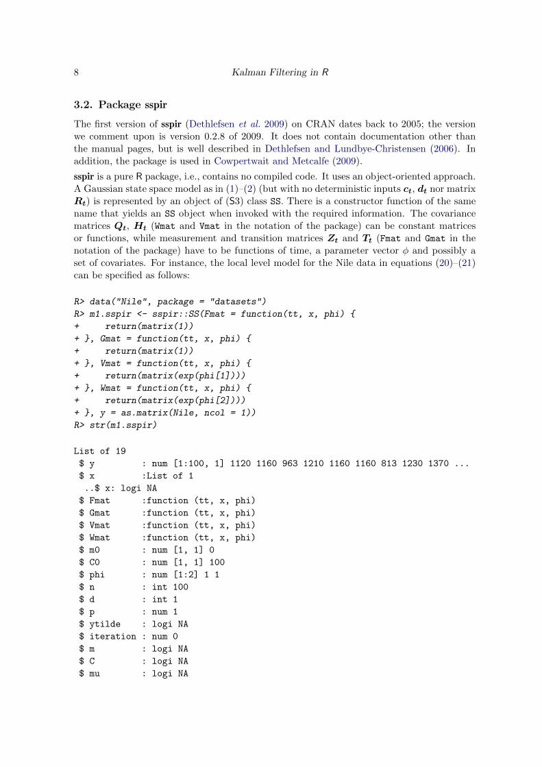
3.2. Package sspir

The first version of sspir (Dethlefsen et al. 2009) on CRAN dates back to 2005; the versionwe comment upon is version 0.2.8 of 2009. It does not contain documentation other thanthe manual pages, but is well described in Dethlefsen and Lundbye-Christensen (2006). Inaddition, the package is used in Cowpertwait and Metcalfe (2009).

sspir is a pure R package, i.e., contains no compiled code. It uses an object-oriented approach.A Gaussian state space model as in (1)–(2) (but with no deterministic inputs ct, dt nor matrixRt) is represented by an object of (S3) class SS. There is a constructor function of the samename that yields an SS object when invoked with the required information. The covariancematrices Qt, Ht (Wmat and Vmat in the notation of the package) can be constant matricesor functions, while measurement and transition matrices Zt and Tt (Fmat and Gmat in thenotation of the package) have to be functions of time, a parameter vector φ and possibly aset of covariates. For instance, the local level model for the Nile data in equations (20)–(21)can be specified as follows:

R> data("Nile", package = "datasets")

R> m1.sspir <- sspir::SS(Fmat = function(tt, x, phi) {

+ return(matrix(1))

+ }, Gmat = function(tt, x, phi) {

+ return(matrix(1))

+ }, Vmat = function(tt, x, phi) {

+ return(matrix(exp(phi[1])))

+ }, Wmat = function(tt, x, phi) {

+ return(matrix(exp(phi[2])))

+ }, y = as.matrix(Nile, ncol = 1))

R> str(m1.sspir)

List of 19

$ y : num [1:100, 1] 1120 1160 963 1210 1160 1160 813 1230 1370 ...

$ x :List of 1

..$ x: logi NA

$ Fmat :function (tt, x, phi)

$ Gmat :function (tt, x, phi)

$ Vmat :function (tt, x, phi)

$ Wmat :function (tt, x, phi)

$ m0 : num [1, 1] 0

$ C0 : num [1, 1] 100

$ phi : num [1:2] 1 1

$ n : int 100

$ d : int 1

$ p : num 1

$ ytilde : logi NA

$ iteration : num 0

$ m : logi NA

$ C : logi NA

$ mu : logi NA


$ likelihood: logi NA

$ loglik : logi NA

- attr(*, "class")= chr "SS"

The constructor yields (in m1.sspir) an object with the passed arguments filled in and someother components (which might also have been specified in the call to SS) set to defaults.Among others, we see y, containing the time series, m0 and C0 (initial mean and covariancematrix of the state vector), phi (vector of parameters), etc. The only two parameters σ2η andσ2ε have been parameterized as exp(φ1) and exp(φ2) to ensure non negativity. A rich set ofaccessor functions allow to get/set individual components in an SS object. For instance, wecan set the initial covariance matrix of the state vector (C0) and the model parameters (phi),

R> C0(m1.sspir) <- matrix(10^7, 1, 1)

R> phi(m1.sspir) <- c(9, 7)

and then inspect their values, as in

R> phi(m1.sspir)

[1] 9 7

Functions kfilter and smoother perform Kalman filtering and smoothing on the SS objectm1.sspir, returning a new SS object with the original information, the filtered (or smoothed)estimates of the state, and their covariance matrices in slots m and C respectively:

R> m1.sspir.f <- kfilter(m1.sspir)

Aside from the use of function SS to set up a state space model, sspir offers a function ssm

based on the familiar formula notation of functions like lm, glm, etc. For instance, the locallevel model for the Nile data could be specified as follows:

R> mod2.sspir <- ssm(Nilo ~ tvar(1), family = "gaussian",

+ C0 = diag(1) * 10^7, phi = exp(c(9, 7)))

R> class(mod2.sspir)

[1] "ssm" "lm"

The returned object is of class ssm. Marker tvar specifies that a right hand side element istime varying (in the example above, the intercept). The family argument can take valuesgaussian, binomial, Gamma, poisson, quasibinomial, quasipoisson and quasi, each withseveral choices of link functions. If gaussian is specified, the function kfs runs the stan-dard Kalman smoother. For a non-Gaussian family, kfs runs an iterated extended Kalmansmoother: it iterates over a sequence of approximating Gaussian models.

Function ssm provides a very convenient user interface, even if it can only be used for uni-variate time series. The use of ssm is further enhanced by ancillary functions like polytrig,polytime, season and sumseason, which help to define polynomial trends and trigonometricpolynomials as well as seasonal dummies.


sspir includes other useful functions for: simulation from a (Gaussian) state-space model(recursion), simulation smoothing (ksimulate) and EM estimation (EMalgo).

Regarding the algorithmic approach followed, sspir implements a covariance filter, with thefaster (8) rather than the more stable (9) update for the state covariance. Somewhat surpris-ingly, missing values are not allowed.

All in all, the design of the package emphasizes usability and flexibility: the fact that systemmatrices can (or need) be specified as functions of time, covariates and parameters affordsunparallelled flexibility. This flexibility has a price, however, as every single use of a matrixforces its recreation from scratch by the underlying function. As we will see in Section 4, this,coupled with the all-R condition of the package, severely impacts performance.

3.3. Package dlm

Version 0.7-1 of package dlm was submitted to CRAN in August 2006. The version we reviewis 1.1-1 (see Petris 2010). Other than the manual pages, an informative vignette accompaniesthe package. A recent book, Petris et al. (2009), provides an introduction to the underlyingtheory and a wealth of examples on the use of the package.

Like sspir, the state-space model considered is a simplified version of (1)–(2), with no in-tercepts ct, dt and no Rt matrix. The emphasis is on Bayesian analysis of dynamic linearmodels (DLMs), but the package can also be used for Kalman filtering/smoothing and maxi-mum likelihood estimation. The design objectives as stated in the concluding remarks of thevignette Petris (2010) are

“. . . flexibility and numerical stability of the filtering, smoothing, and likelihoodevaluation algorithms. These two goals are somewhat related, since naive imple-mentations of the Kalman filter are known to suffer from numerical instabilityfor general DLMs. Therefore, in an environment where the user is free to specifyvirtually any type of DLM, it was important to try to avoid as much as possiblethe aforementioned instability problems.”

In order to cope with numerical instability, the author of the package has chosen to implementa form of square root filter described in Zhang and Li (1996), which propagates factors of thesingular value decomposition (SVD) of Pt. It is claimed that the algorithm is more robustand general than standard square root filters. The computation is done in C, with extensiveuse of LAPACK routines. Initial conditions a0|−1 and P0|−1 have to be specified (or thedefaults accepted). There is no provision for exact initial diffuse conditions.

Aside from the heavy duty compiled functions, the package provides a rich set of interfacefunctions in R, to help with the specification of state-space models. A time-invariant modelis an object of (S3) class "dlm". A general constructor is provided, not unlike SS in packagesspir, which returns a dlm object when invoked with arguments V, W (covariance matrices ofthe measurement and state equations, respectively), FF and GG (measurement equation matrixand transition matrix respectively), and m0, C0 (prior mean and covariance matrix of the statevector). For instance,

R> m1.dlm <- dlm(FF = 1, V = 0.8, GG = 1, W = 0.1, m0 = 0, C0 = 100)

creates a dlm object representing the model in (20)–(21) with σ2ε = 0.8 and σ2η = 0.1. Theclass and structure of the object is


R> str(m1.dlm)

List of 6

$ m0: num 0

$ C0: num [1, 1] 100

$ FF: num [1, 1] 1

$ V : num [1, 1] 0.8

$ GG: num [1, 1] 1

$ W : num [1, 1] 0.1

- attr(*, "class")= chr "dlm"

Much as in sspir, there is a full complement of functions to get/set specific components ofdlm class objects.

Time-varying system matrices and covariates are handled in a manner reminiscent of theapproach used in SSFPack (Koopman et al. 1999). Whenever one of the matrices FF, GG, V orW has time-varying elements, we have to specify a similarly sized matrix JFF, JGG, JV or JW

with zeros in the places of time invariant elements and a positive integer otherwise. If entryJFF[i,j] is set to k, that means that at time s FF[i,j] is equal to X[s,k]. For instance,assuming y is an N length vector of observations and X an N ×2 matrix of covariates, a linearregression model

yt = β0t + β1tX1t + β2tX2t + εt (22)

in which all β’s are allowed to change over time following a random walk dynamics withσ2β0 = σ2β1 = σ2β2 = 0.1, could be specified as follows:

R> m2.dlm <- dlm(FF = matrix(c(1, 0, 0), 1, 3),

+ JFF = matrix(c(0, 1, 2), 1, 3), GG = diag(3), W = 0.1 * diag(3),

+ V = 4, m0 = c(0, 0, 0), C0 = 10^9 * diag(3), X = X)

Unlike with sspir’s objects of class SS, the series of observations is not included in the dlm

object.

sspir enhanced usability with the ssm function interface and ancillary functions to create com-mon patterns in the system matrices. dlm has ancillary functions dlmModARMA, dlmModPoly,dlmModReg, dlmModSeas and dlmModTrig, which help with ARMA, polynomial trends, re-gression terms and seasonal components in two different forms. For instance, we might use

R> m3.dlm <- dlmModARMA(ar = c(0.3, 0.2, 0.4), ma = c(0.9, 0.1))

R> m3.dlm

$FF

[,1] [,2] [,3]

[1,] 1 0 0

$V

[,1]

[1,] 0


$GG

[,1] [,2] [,3]

[1,] 0.3 1 0

[2,] 0.2 0 1

[3,] 0.4 0 0

$W

[,1] [,2] [,3]

[1,] 1.0 0.90 0.10

[2,] 0.9 0.81 0.09

[3,] 0.1 0.09 0.01

$m0

[1] 0 0 0

$C0

[,1] [,2] [,3]

[1,] 1e+07 0e+00 0e+00

[2,] 0e+00 1e+07 0e+00

[3,] 0e+00 0e+00 1e+07

for an ARMA(3,2) model (the ar= and ma= arguments could be lists of matrices, so multi-variate time series can be handled just as easily).

While dlm does not offer a function like ssm allowing simple formula notation, it implementsa very powerful mechanism which greatly eases the creation of system matrices. Genericoperator ’+’ has been overloaded to “add” model components into a comprehensive modelfor a time series. Thus, one can write

R> m4.dlm <- dlmModPoly(order = 1) + dlmModSeas(4)

to create a local level plus (period 4) seasonal model.

In addition, a new “outer sum” operator has been defined on dlm objects that combinesmodels for different time series into a joint model. This eases the definition of models inwhich different components have different dynamics. For instance, m3.dlm and m4.dlm couldbe combined as in:

R> m3Plusm4.dlm <- m4.dlm %+% m3.dlm

This yields a bivariate time series model, where the first component follows a local level plusseasonal dynamics, while the second is an ARMA(3,2), with a state vector of total dimensiond = 7. The transition matrix is

R> GG(m3Plusm4.dlm)

[,1] [,2] [,3] [,4] [,5] [,6] [,7]

[1,] 1 0 0 0 0.0 0 0

[2,] 0 -1 -1 -1 0.0 0 0


[3,] 0 1 0 0 0.0 0 0

[4,] 0 0 1 0 0.0 0 0

[5,] 0 0 0 0 0.3 1 0

[6,] 0 0 0 0 0.2 0 1

[7,] 0 0 0 0 0.4 0 0

and the observation matrix

R> FF(m3Plusm4.dlm)

[,1] [,2] [,3] [,4] [,5] [,6] [,7]

[1,] 1 1 0 0 0 0 0

[2,] 0 0 0 0 1 0 0

It is assumed that the blocks “added” are independent, but the resulting dlm object can beamended if they are not. Both the overloaded generic + and %+% are real productivity boosters.

Maximum likelihood estimation of the Gaussian model is handled by function dlmMLE: itrequires as arguments a vector of parameters and a function which builds the state spacemodel for the given values of the parameters, and then invokes the standard optimizingfunction optim.

Package dlm is geared towards Bayesian analysis of time series, and offers facilities which goway beyond what we have described. For a fuller account, the reader is referred to Petriset al. (2009).

3.4. Package FKF

Package FKF (Luethi et al. 2010) first appeared on CRAN in February 2009; the version wecomment upon is version 0.1.0. The name of the package stands for “Fast Kalman Filter”,and emphasis is on speed. From the DESCRIPTION file,

“Due to the speed of the filter, the fitting of high-dimensional linear state spacemodels to large datasets becomes possible.”

It contains only two functions, fkf and plot.fkf. The second is an ancillary function to plotfiltering results. fkf is a wrap envelope in R of a C routine implementing the filter. The statespace model considered is as described by equations (1)–(2) with an added input matrix St

in the measurement equation, which is thus

yt = dt +Ztαt + Stεt. (23)

All system matrices ct, Tt, dt, Zt, Qt, St and Ht may be constant or time varying. Thelatter case requires their definition as three dimensional arrays, the last dimension being time.

Aside from doing all computations in compiled code, the authors have chosen to use a co-variance filter rather than a square root filter, consistent with their quest of maximum speed:they code equations (5)–(8) almost verbatim.

Computation is multivariate, i.e., they do not take advantage of sequential processing – whichfor large dimensions of the observation vector yt and diagonal Ht might offer substantial


advantages. Rather, they focus on fast linear algebra computations, with extensive resort toBLAS and LAPACK routines. Not using the sequential approach makes it harder to dealwith scattered missing values in vector yt, which were not supported in previous versions ofthe package (but are as of version 0.1.0)

Function fkf computes and returns the likelihood, as in equation (15). Computation of thelikelihood is stopped if Ft happens to be singular, something which should never be thecase for positive definite matrices Ht. Function fkf returns both filtered at and predictedat|t−1 estimations of the state. It makes no provision, though, for smoothed values at|N norsimulation smoothing.

While limited in the scope of the facilities it offers, FKF excels in the speed of the filter, aswill be apparent in the examples shown later.

3.5. Package KFAS

Package KFAS (Helske 2010) is the most recent addition to Kalman filtering in R. It includesfunctions for Kalman filtering, smoothing, simulation smoothing and disturbance smoothing.It also includes an ancillary function to forecast from the output of the Kalman filter. Themodel supported is (1)–(2), except for ct and dt.

The package follows closely Durbin and Koopman (2001) and papers by the same authors(Koopman and Durbin 2003, 2000) implementing algorithms as presented in those references.Time varying system matrices are supported, as are missing values. The R functions do someerror checking and call Fortran 90 routines which perform most of the computational effort;extensive use is made of BLAS and LAPACK for all linear algebra computations. As in thecase of the preceding package, time-varying matrices are handled by using three dimensionalarrays, the last dimension being time. The package contains seven user visible functions: kf,ks, simsmoother, distsmoother, eflik/eflik0 and forecast for, respectively, Kalman fil-tering, smoothing, simulation smoothing, disturbance smoothing, approximate log-likelihoodcomputation of non-Gaussian models and forecasting.

One of the characteristics that set this package apart is the use of sequential processing(Section 2.3 above). Aside from the expected performance advantages when the dimensionof yt is large, this approach makes it easy to deal with irregularly missing entries: they aresimply dropped from yt (and so are the corresponding rows of Zt and rows and columns ofHt)

Sequential processing requires that the components of yt be uncorrelated or else that the“decorrelation” described just prior to equation (14) is carried out. This is done by the kf

function which at each step of the Kalman filter iteration, checks for diagonality Ht (or asub-matrix Ht, if some rows and columns have been dropped on account of missing valuesin yt). If it is not diagonal, the observation equation is transformed to a form like (14) bymultiplying by a square root of Ht

−1 (or H−1t ): a Cholesky factor is used, in the case of full

rank), and the resulting y∗t is processed one element at a time.

Another feature that sets this package apart is the use of exact initial diffuse conditions a laDurbin and Koopman (2001). Function kf can be supplied with a proper initial distributionor an exact diffuse initialization for some or all of the elements of the initial state vector.

Although processing data sequentially, KFAS still implements a standard covariance filter,much as in equations (5)–(8).


3.6. Other functions performing Kalman filtering

There are functions in other R packages which cater to particular cases of state space models.The function StructTS by B.D. Ripley in recommended package stats fits basic structuralmodels (see Harvey (1989)) to univariate time series. It is quite reliable and fast, and is usedas a benchmark in some of the comparisons that follow in Section 4. (Functions KalmanLike,KalmanRun, KalmanSmooth and KalmanForecast in the same package stats can also be used,although are not intended to be called directly, but rather by other functions.) Package Stem(Cameletti 2009) includes Stem.Model and Stem.Estimation functions, specifying and fitting(using a EM algorithm, entirely coded in R) a particular spatio-temporal model. Kalmanfiltering and smoothing routines are present also in other packages, including timsac (TheInstitute of Statistical Mathematics 2009) and cts (Tunnicliffe-Wilson and Wang 2006).

4. Features and speed comparison

4.1. Features

A brief description of some of the capabilities of each package has been given in the precedingsection. Table 1 is provided as a quick summary, by no means complete. It should beunderstood, on the other hand, that some features can be easily implemented even if notalready coded in the package. For instance, maximum likelihood estimation only requires afew lines of code once we have a routine which computes the likelihood of the state spacemodel (which all packages provide).

dse sspir dlm FKF KFAS2009.10-2 0.2.8 1.1-1 0.1.0 0.6.0

Coded in: R + Fortran R R + C R + C R + FortranClass model (if any) S3 S3 S3 S3Algorithm CF CF SRCF CF CFSequential processing

√

Exact diffuse initialization√

Missing values in yt allowed√ √ √

Time varying matrices√ √ √ √

Simulator√ √

Smoother√ √ √ √

Simulation smoother√ √ √

Disturbance smoother√

MLE routine√ √ √

Non-Gaussian models√ √

Table 1: Feature comparison of five packages performing Kalman filtering. CF = Covariancefilter, SRCF = Square root covariance filter.


4.2. Speed comparison

In order to assess the relative speed of the four packages examined, we have conducted a fewexperiments. In all of them we have estimated parameters in Gaussian models of differentsizes by maximum likelihood. This requires repeated runs of the Kalman filter and has beendone either using a function provided in the package (e.g., dlmMLE in package dlm) or writinga small function which computes the log likelihood (using the Kalman filtering routine in eachpackage) and then handing over that likelihood to function optim for optimization.

The following data sets have been used in the experiments:

Nile data. This is the well-known Nile data described in Durbin and Koopman (2001)and referred to earlier. It is a short (N = 100 observations) univariate time series. A locallevel model involving just two parameters (σ2η and σ2ε , variances of the innovation and themeasurement noise) has been fitted by maximum likelihood, with all four packages and withfunction StructTS.

Exchange rates data. Data consists of N = 2465 daily observations of the exchange rate(against the US dollar, USD) of four currencies (AUD, BEF, CHF and DEM), for the periodfrom 1988-01-04 to 1997-08-15. Their joint evolution is displayed in Figure 1

Regression artificial data. The data consists of N = 1000 artificially generated observa-tions from the linear model yt = β1X1 + . . . + β5X5 + ε, with βi = i for i = 1, . . . , 5. Thevector β can be thought of as an invariant state vector (i.e., Qt = 0). The model can beestimated by ordinary least squares and sequentially, by means of the Kalman filter. Thepurpose of this experiment was to check the accuracy of the algorithms in an example withQt = 0, which might expose numerical instability when equations (6) and (8) are used.

Results. The benchmarks were run on a 2GHz. Xeon machine, running Linux and Rcompiled for 64 bits with an optimized BLAS library (ATLAS, see Whaley et al. 2001). Amachine using a non-optimized library might see different relative performances, as some ofthe packages rely very heavily on BLAS. We have selected algorithm L-BFGS-B, Byrd et al.(1995), as coded in function optim in R. The feasible region for parameters (non-negativehalf line for variances, (−1, 1) for correlation coefficients) has been specified in the call tooptim. When coding bounds for variances or correlation coefficients, we found that we had toforce parameters to be slightly away from the boundary of the feasible region: lower bounds of10−6 were given for variances and a feasible interval of (−0.99, 0.99) for correlation coefficients.Common initial values, tolerance and scaling have been used for each experiment with all fourpackages.

The list of models fitted and the times taken are summarized in Table 2, which we commentbriefly next.

In the case of the Nile example (local level model fitted to a short univariate series), theinterpreted nature of the sspir is seen taxing its performance very heavily: it takes much longerthan the second slowest package. Even among the packages implementing the Kalman filter incompiled code, there are noticeable differences, FKF being clearly the fastest. Interestingly,


Date

Uni

ts p

er U

S d

olla

r

1.4

1.6

1.8

2.0

DEM1.

21.

41.

61.

8

CHF

3035

40

BEF

0.7

0.8

0.9

1988 1990 1992 1994 1996 1998

AUD

Figure 1: Daily exchange rate against the US dollar (USD) of the Australian dollar (AUD),Belgian franc (BEF), Swiss franc (CHF) and German mark (DEM). Period 1988-01-04 to1997-08-15.

in spite of using a type of square root algorithm (SVD factorization), dlm ends up being aboutas fast as KFAS in this particular example.

The Nile example is a particular case of structural model, which can be fit most convenientlyusing function StrucTS. Calling,

R> fit <- StructTS(Nile, type = "level")

returns the local level model fit in about 0.02 seconds!

For the exchange rates data, we have considered p-variate subsets with p = 2, 3 and 4 cur-rencies, to see the performance of the different packages as the dimension of the observationvector increases (and in particular to assess the benefits afforded by the sequential approachused in package KFAS). To each p-variate time series of length N = 2465 we have fitted atime-invariant local level model. Observations are assumed contemporaneously correlated,


sspir dlm FKF KFAS

proper diffuse

I. Nile exampleLocal level model(p = 1, d = 1, N = 100)

10.13 0.17 0.07 0.17 0.15

II. Exchange rates exampleLocal level modelVt equicorrelated(p = 2, d = 2, N = 2465)

1058.22 19.28 7.40 6.63 6.44

III. Exchange rates exampleLocal level modelVt equicorrelated(p = 3, d = 3, N = 2465)

4105.41 117.32 27.50 47.76 74.69

IV. Exchange rates exampleLocal level modelVt equicorrelated(p = 4, d = 4, N = 2465)

6853.85 264.25 64.89 122.15 98.67

V. Exchange rates exampleSingle factor modelVt diagonal(p = 3, d = 1, N = 2465)

3334.48 62.68 31.41‡ 21.17 19.60

VI. Regression modelQt = 0(p = 1, d = 5, N = 1000)

8.52 1.13 0.23 0.48 0.28

Table 2: Times in seconds for the maximum likelihood estimation of the models indicated.p, d,N are respectively the dimension of yt, the dimension of the state vector and the lengthof time series. Symbol ‡ marks abnormal exit in the optimization routine; see text.

with pairwise common correlation ρ: Vt has p distinct variances along the main diagonal andoff-diagonal (i, j) element of the form σiσjρ for all (i, j). We have assumed the disturbancedriving the state vector to have a diagonal covariance matrix Qt. Thus, we have 2p + 1parameters: p variances in each of Vt and Qt plus ρ. (We are not claiming that this modelis anywhere close to optimal for the data at hand, although one could find some rationale forit.)

For the series BEF, CHF and DEM, with a very similar evolution with respect to the US$(see Figure 1), we have also considered a dynamic single factor model,

yt = Ztαt + εt (24)

αt = αt−1 + ηt. (25)

Matrices Tt and Vt are assumed time invariant, with Vt diagonal. (This is the best scenariofor sequential processing, which benefits from large p relative to d and uncorrelated inputs.)


Thus, there are six parameters to estimate: three variances in Vt plus σ2η and two parametersin Tt (the first entry in Tt has been set to 1 to insure identifiability).

In all cases, a common set of starting values has been used with all the packages, roughly withinan order of magnitude of the optima found. Not only the starting values were important, butalso the scaling, which took some trial and error to set.

We see again that the interpreted nature of the Kalman filter routine in sspir exacts a heavytoll on performance, with running times from 50 to over a hundred times longer than thoseof the other packages. It is not only that code is interpreted, but also there is heavy overheadfrom repeated function calls: each iteration of the Kalman filter calls a filterstep function.Likewise, the likelihood term of (15) computed at each iteration requires an additional functioncall, which incurs further overhead by checking formal consistency of its arguments over andover again.

With one of the models, when optimizing a likelihood computed with package FKF, optimstopped with a message ERROR: ABNORMAL_TERMINATION_IN_LNSRCH: the returned values ofthe parameters where in close agreement, though, with those returned when using sspir, dlmor KFAS.

We ran many more experiments, including in the data set exchange rates for more currencies,up to twelve at a time: the Vt-equicorrelated local level model then has 12 + 12 + 1 freeparameters. In general, with dimensions larger than those reported in Table 2, attempts to fitmodels by maximum likelihood were quite sensitive to the starting values and scaling suppliedto optim, frequently unsuccessful and always costly.

Based only on the results reported in Table 2, we can conclude that FKF is fastest, by a factorof about 2, except in example II, where KFAS is slightly faster, and example V where it issignificantly faster. In turn, KFAS is faster than dlm by a factor between 2 and 3. Contraryto our initial expectation, the use of an exact diffuse initialization in KFAS does not seem toadd to the running time.

Examples such as those in Table 2 are interesting in that they give timings for a commontask in time series analysis – maximum likelihood estimation of a model. However, thosetimes only partially reflect the relative performance of the Kalman filtering routines, as theyinclude the running time of the optimizing routine – in our case, optim.

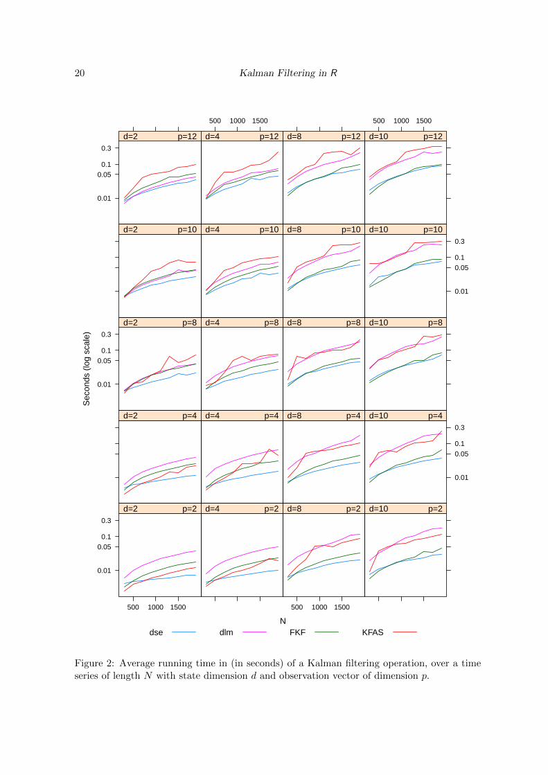
To better assess the relative speed of the different Kalman filter routines, we can run themon time series of different lengths, with varying state and measurement dimensions. We haveexcluded from the comparison package sspir, whose running times are clearly in a differentcategory. On the other hand, we have included dse, which was not included in Table 2 becauseit computes the likelihood in a different manner, and hence does not reach the same optimaas the rest of the packages.

The results can be seen in Figure 2. We have used multivariate random walks of length N =300 to 1900, state dimensions d = 2, 4, 8 and 12 and measurements of dimension p = 2, 4, 8, 10and 12. Timings have been obtained by averaging the total time of 25 runs using the functionsystem.time.

The timing method is not very accurate, even after averaging 25 different realizations. Spe-cially annoying is the fact that some of the timings do not monotonically increase with N , asone would expect. (Prior to each set of 25 Kalman filter runs, a garbage collection was forced,to minimize the chance that it be automatically called within the timed loop. We may havebeen unsuccessful at preventing such undesired garbage collections in all cases.) Nonetheless,


N

Sec

onds

(lo

g sc

ale)

0.01

0.050.1

0.3

500 1000 1500

d=2 p=2 d=4 p=2

500 1000 1500

d=8 p=2 d=10 p=2

d=2 p=4 d=4 p=4 d=8 p=4

0.01

0.05

0.1

0.3

d=10 p=4

0.01

0.050.1

0.3

d=2 p=8 d=4 p=8 d=8 p=8 d=10 p=8

d=2 p=10 d=4 p=10 d=8 p=10

0.01

0.050.1

0.3

d=10 p=10

0.01

0.050.1

0.3

d=2 p=12

500 1000 1500

d=4 p=12 d=8 p=12

500 1000 1500

d=10 p=12

dse dlm FKF KFAS

Figure 2: Average running time in (in seconds) of a Kalman filtering operation, over a timeseries of length N with state dimension d and observation vector of dimension p.


KFAS

True βi OLS sspir dlm FKF proper diffuse

1.000000 1.052865 1.052864 1.052864 1.052864 1.052864 1.0528652.000000 2.006062 2.006060 2.006060 2.006060 2.006060 2.0060623.000000 2.996563 2.996559 2.996559 2.996559 2.996559 2.9965634.000000 4.061145 4.061140 4.061140 4.061140 4.061140 4.0611455.000000 4.988728 4.988723 4.988723 4.988723 4.988723 4.988728

Table 3: Real and estimated parameter values in the regression example with N = 1000.The OLS column displays the estimated values of the betas by ordinary least squares. Theremaining columns show the estimates using the Kalman filter as implemented by the fourpackages with initialization a0 = 0, P0 = 1000× I or exact diffuse (last column).

the patterns in Figure 2 are clear: for most combinations of state and measurement dimensionand most series lengths, FKF and dse Kalman filtering routines come out fastest. dlm is ingeneral about 4-5 times slower (note the log scale in Figure 1), as one would expect giventhe greater computational effort demanded by the square root algorithm it uses; however, forsmall state dimensions and relatively large measurement dimensions, it does quite well, withperformances close to FKF and dse.

Unexpectedly, KFAS, which one would expect to improve relatively to the others when p islarge, displays the opposite effect, at least for small d: as we go upwards in the first andsecond columns of Figure 1, the performance of KFAS degrades relatively to the others. Formodels with larger state dimension (d = 8 and d = 10), timings for KFAS are close to thoseof dlm, and both considerably above those of dse and FKF.

It is important to realize, though, that routines in different packages produce more or lesscomprehensive outputs, which in part accounts for their different running times. It shouldalso be borne in mind packages like dse which assume time-invariant system matrices, aregiven an advantage over those which make allowance for time-varying matrices (incurring theoverhead of three rather than two index arrays, the third index for time).

Besides looking at the running times, it is interesting to compare results in the estimatedparameters.

Table 3 shows the estimated betas in the regression example (VI in Table 2). All four packages,when run with the same initial conditions, produce results which match to 5-6 decimal places.Function kf in package KFAS, when run with exact diffuse initial conditions, produces slightlydifferent results. All estimations are in good agreement with those obtained by ordinary leastsquares, as it should be (see Eubank 2006, Section 6.3).

The differences in the estimated values when exact initial diffuse conditions and approximatediffuse conditions were used, are quite small, as is in general the case with “long” time series.This is not always so: on the issue of fitting structural models and the impact of initialconditions Ripley (2002) gives some insightful comments.

Agreement among the estimates produced by the different packages is not quite so good inthe other experiments, but estimates are still close. For the case of the single factor modelfitted to the currencies exchange rates (V in Table 2) we can see the results in Table 4. Somediscrepancies among estimates computed by the different packages can be seen starting at the


Estimated by:

Parameter sspir dlm FKF KFAS

V11 × 105 7.345022 7.329658 7.336880 7.331016V22 × 103 1.154476 1.145747 1.184988 1.145720V33 × 106 3.614857 3.623933 3.592682 3.625587Z21 1.055430 1.054714 1.054527 1.054738Z23 0.942436 0.942302 0.942290 0.942294σ2η × 105 4.585722 4.600876 4.603320 4.599717

sspir `(θ) 21780.17 21780.22 21779.52 21780.23dlm −`(θ) -28575.72 -28575.77 -28575.08 -28575.77FKF `(θ) 21780.18 21780.22 21779.54 21780.22KFAS `(θ) 28575.72 28575.77 28575.08 28575.77

Table 4: Estimates of parameters for the currency exchange rates single factor model, suitablyscaled. Last four rows report the (minus) log likelihood `(θ) of each set of estimates usingthe Kalman filter routines of all four packages.

second significant digit.

The last four rows of Table 4 display the log likelihood evaluated by each of the four packagesat the parameter values directly above. (This allows comparison of the four sets of estimates interms of the log likelihood as computed by any of the four packages.) There is good agreementamong the values in each row (not between rows, as some packages compute the likelihoodup to a constant term). If anything, it looks as if the parameter estimates computed by FKFgive a slightly lower log likelihood, whichever package is used to evaluate it, but the differenceis hardly of any consequence.

5. Discussion

R now offers a choice of packages for state space modelling and estimation. Each package hasdifferent strengths and emphasizes different tasks.

Both sspir and dlm offer a nice user interface, following different approaches. For univariatetime series, the formula interface of sspir may be the easiest and fastest to learn and use.The approach taken in dlm is quite general and elegant and enables the user to build a model“adding” blocks with the redefined ’+’ operator and the outer sum %+%. Both offer ancillaryfunctions to help in the model specification task.

Packages FKF and KFAS offer a much more austere interface: the user is left alone to producethe inputs to the filtering routines. FKF is indisputably fastest. KFAS offers a rich set offunctions for filtering, smoothing, simulation smoothing, etc. and has quite acceptable speed.It is unique in offering exact initial diffuse conditions for all or part of the components in thestate vector: all other packages resort to a “vague” proper a priori distribution for the initialstate vector when there is no a priori information.

KFAS is also unique in its sequential processing approach, although in the examples examinedthis did not appear to give it an advantage. It is possible that the need to “decorrelate”


the inputs partly offsets the advantages of sequential processing. It is also possible, giventhe extensive use of BLAS routines for all vector and matrix operations, that the increasednumber of calls (by a factor of p, the dimension of yt) pushes overhead which partially negatesthe greater efficiency of sequential processing.

dse and FKF provide the fastest Kalman filtering routines, although in the former case neithermissing values nor time-varying system matrices are supported.

Algorithm wise, dlm is the only one to use a form of square root algorithm, based on thesingular value decomposition of the covariance matrix of the state vector. It has performedquite reliably in the examples reported and others. Even though it uses an algorithm requiringin principle more effort than a standard covariance filter, it takes only about 2-3 times longerthan KFAS in the examples reported in Table 2.

We expected the choice of algorithm to have a greater impact, particularly since the covariancefilter implemented by sspir, FKF and KFAS does not make use of (9), but rather of (8). Asit happens, the parameter estimation results in the regression example check to 5-6 decimalplaces, and in the other examples run we found differences only after the second decimal place,like those reported in Table 4. When the likelihood optimization does not stop abnormally,the four packages appear to give results equivalent for all practical purposes.

We found occasional problems when one or several parameters approached the feasibilityboundary. This is quite common with basic structural models, where one or more noisevariances are frequently estimated at zero (cf. Ripley (2002)).

Although the packages analyzed are already of high quality, there is room for improvement.We have mentioned before the approach taken by sspir resorting extensively to function callswhich make the code modular and easy to read, but add overhead. In the compiled code ofthe other packages, there could be a case for inlining some operations presently handled byBLAS calls. Above all, achieving speeds of the kind exhibited by function StructTS probablyrequires code which handles different problems differently. For instance, the (quite common)case of a time invariant Tt (or Ft) equal to the unit matrix simplifies the transition fromat|t−1 to at in Equation 5, saving a matrix multiplication (and further simplifications wouldbe realized in Equation 6). Similar savings can be realized with specialized code for otheroften-occurring particular cases of sparse transition matrices.

As a further example, time varying system matrices are implemented, e.g., in KFAS, by threedimensional arrays, the third index being time. In the event of, say, two regimes requiringsome of the system matrices to have one of two “states”, we have nevertheless to fill the entirethree dimension array, with third dimension equal to N , the length of the series.

This may be relatively innocuous efficiency wise: but if the time varying matrix is Vt andhappens to be non-diagonal, we will be decorrelating the inputs over and over again – andthis may be quite time consuming.

At the time being, most users will probably want to use more than one of the packagesexamined. However uncomfortable it may be at times, this allows the user to reap the benefitsfrom the best features of each package, and have access to open source tools for state spacemodelling and estimation that could only be dreamt of a few years back.


Acknowledgments

I am indebted to the authors of the packages mentioned above (Paul Gilbert, Claus Dethlefsen,Giovannis Petris, David Luthi and Jouni Helske), for help, comments or clarifications offeredat various points in time. I am also indebted for comments to Ignacio Dıaz-Emparanza, twoanonymous referees and the editor of the journal. The usual disclaimer applies. Partial sup-port from grants ECO2008-05622 (MCyT) and IT-347-10 (Basque Government) is gratefullyacknowledged.

References

Anderson BDO, Moore JB (1979). Optimal Filtering. Prentice-Hall.

Anderson E, Bai Z, Bischof C, Blackford S, Demmel J, Dongarra J, Croz JD, GreenbaumA, Hammarling S, McKenney A, Sorensen D (1999). LAPACK Users’ Guide. 3rd edition.SIAM.

Bierman GJ (1977). Factorization Methods for Discrete Sequential Estimation. Dover Publi-cations.

Bucy RS, Joseph PD (1968). Filtering for Stochastic Processes with Application to Guidance.Interscience, New York.

Byrd RH, Lu P, Nocedal J, Zhu C (1995). “A Limited Memory Algorithm for Bound Con-strained Optimization.” SIAM Journal on Scientific Computing, 16, 1190–.1208.

Cameletti M (2009). Stem: Spatio-Temporal Models in R. R package version 1.0, URLhttp://CRAN.R-project.org/package=Stem.

Carter CK, Kohn R (1994). “On Gibbs Sampling for State Space Models.” Biometrika, 81(3),541–553.

Chambers JM (2008). Software for Data Analysis: Programming with R. Springer-Verlag,New York.

Chambers JM, Hastie TJ (1992). Statistical Models in S. Wadsworth & Brooks/Cole, PacificGrove.

Cowpertwait PSP, Metcalfe AV (2009). Introductory Time Series with R. Springer-Verlag,New York.

de Jong P (1995). “The Simulation Smoother for Time Series Models.” Biometrika, 82(2),339–350.

Dethlefsen C, Lundbye-Christensen S (2006). “Formulating State Space Models in R withFocus on Longitudinal Regression Models.” Journal of Statistical Software, 16(1), 1–15.URL http://www.jstatsoft.org/v16/i01/.

Dethlefsen C, Lundbye-Christensen S, Christensen AL (2009). sspir: State Space Models inR. R package version 0.2.8, URL http://CRAN.R-project.org/package=sspir.

http://CRAN.R-project.org/package=Stem

http://www.jstatsoft.org/v16/i01/

http://CRAN.R-project.org/package=sspir


Durbin J, Koopman SJ (2001). Time Series Analysis by State Space Methods. Oxford Uni-versity Press, New York.

Durbin J, Koopman SJ (2002). “A Simple and Efficient Simulation Smoother for State SpaceTime Series Analysis.” Biometrika, 89(3), 603–615.

Eubank RL (2006). A Kalman Filter Primer. Chapman & Hall/CRC.

Fruhwirth-Schnatter S (1994). “Data Augmentation and Dynamic Linear Models.” Journalof Time Series Analysis, 15(2), 183–202.

Gentle JE (2007). Matrix Algebra: Theory, Computations, and Applications in Statistics.Springer-Verlag, New York.

Gilbert P (2010). EvalEst: Dynamic Systems Estimation – Extensions. R package ver-sion 2010.02-1, URL http://CRAN.R-project.org/package=EvalEst.

Gilbert PD (1993). “State Space and ARMA Models: An Overview of the Equivalence.”Technical Report 94-3, Bank of Canada. URL http://www.bank-banque-canada.ca/

pgilbert/.

Gilbert PD (2011). Brief User’s Guide: Dynamic Systems Estimation. R package vignette,version 2009.12-1, URL http://CRAN.R-project.org/package=dse.

Grewal MS, Andrews A (2001). Kalman Filtering : Theory and Practice Using MATLAB.Second edition. John Wiley & Sons. ISBN 0-471-39254-5.

Harvey AC (1989). Forecasting, Structural Time Series Models and the Kalman Filter. Cam-bridge University Press, Cambridge.

Helske J (2010). KFAS: Kalman Filter and Smoothers for Exponential Family State SpaceModels. R package version 0.6.0, URL http://CRAN.R-project.org/package=KFAS.

Koopman S, Durbin J (2000). “Fast Filtering and Smoothing for Non-Stationary Time SeriesModels.” Journal of the American Statistical Association, 92, 1630–1638.

Koopman SJ (1997). “Exact Initial Kalman Filtering and Smoothing for Nonstationary TimeSeries Models.” Journal of the American Statistical Association, 92(440), 1630–1638.

Koopman SJ, Durbin J (2003). “Filtering and Smoothing of State Vector for Diffuse State-Space Models.” Journal of Time Series Analysis, 24(1), 85–98.

Koopman SJ, Shephard N, Doornik J (1999). “Statistical Algorithms for Models in StateSpace Using SsfPack 2.2.” Econometrics Journal, 2, 113–166.

Lawson CL, Hanson RJ (1974). Solving Least Squares Problems. Prentice-Hall, EnglewoodCliffs.

Luethi D, Erb P, Otziger S (2010). FKF: Fast Kalman Filter. R package version 0.1.1, URLhttp://CRAN.R-project.org/package=FKF.

Petris G (2010). “An R Package for Dynamic Linear Models.” Journal of Statistical Software,36(12), 1–16. URL http://www.jstatsoft.org/v36/i12/.

http://CRAN.R-project.org/package=EvalEst

http://www.bank-banque-canada.ca/pgilbert/

http://www.bank-banque-canada.ca/pgilbert/

http://CRAN.R-project.org/package=dse

http://CRAN.R-project.org/package=KFAS

http://CRAN.R-project.org/package=FKF

http://www.jstatsoft.org/v36/i12/


Petris G, Petrone S, Campagnoli P (2009). Dynamic Linear Models with R. Springer-Verlag,New York.

R Development Core Team (2010). R: A Language and Environment for Statistical Computing.R Foundation for Statistical Computing, Vienna, Austria. ISBN 3-900051-07-0, URL http:

//www.R-project.org/.

Ripley BD (2002). “Time Series in R 1.5.0.” R News, 2(2), 2–7. URL http://CRAN.

R-project.org/doc/Rnews/.

Schweppe FC (1965). “Evaluation of Likelihood Functions for Gaussian Signals.” InformationTheory, 11, 61–70.

Shumway RH, Stoffer DS (2006). Time Series Analysis and Its Applications – With R Exam-ples. Springer-Verlag, New York.

Simon D (2006). Optimal State Estimation: Kalman, H Infinity, and Nonlinear Approaches.John Wiley & Sons.

Strickland CM, Turner IW, Denham R, Mengersen KL (2009). “Efficient Bayesian Estimationof Multivariate State Space Models.” Computational Statistics & Data Analysis, 53, 4116–4125.

The Institute of Statistical Mathematics (2009). timsac: Time Series Analysis and ControlPackage. R package version 1.2.1, URL http://CRAN.R-project.org/package=timsac.

Tunnicliffe-Wilson G, Wang Z (2006). cts: Continuous Time Autoregressive Models. R pack-age version 1.0-1, URL http://CRAN.R-project.org/src/contrib/Archive/cts/.

Vanbegin M, Verhaegen M (1989). “Algorithm 675: Fortran Subroutines for Computing theSquare Root Covariance Filter and Square Root Information Filter in Dense or HessenbergForms.” ACM Transactions on Mathematical Software, 15(3), 243–256.

West M, Harrison J (1997). Bayesian Forecasting and Dynamic Models. Springer-Verlag, NewYork.

Whaley RC, Petitet A, Dongarra JJ (2001). “Automated Empirical Optimizations of Softwareand the ATLAS Project.” Parallel Computing, 27(1–2), 3–35.

Zhang Y, Li XR (1996). “Fixed-Interval Smoothing Algorithm Based on Singular ValueDecomposition.” In Proceedings of the 1996 IEEE International Conference on ControlApplications, pp. 916–921.

Affiliation:

Fernando TusellDepartment of Statistics and Econometrics (EA-III)Facultad de CC.EE. y Emp. – UPV/EHU

http://www.R-project.org/

http://www.R-project.org/

http://CRAN.R-project.org/doc/Rnews/

http://CRAN.R-project.org/doc/Rnews/

http://CRAN.R-project.org/package=timsac

http://CRAN.R-project.org/src/contrib/Archive/cts/


Avda. Lehendakari Aguirre, 83E-48015 Bilbao, SpainE-mail: [email protected]: http://www.et.bs.ehu.es/~etptupaf/

Journal of Statistical Software http://www.jstatsoft.org/

published by the American Statistical Association http://www.amstat.org/

Volume 39, Issue 2 Submitted: 2010-01-12March 2011 Accepted: 2010-08-17

mailto:[email protected]

http://www.et.bs.ehu.es/~etptupaf/

http://www.jstatsoft.org/

http://www.amstat.org/

kalman filtering in r - connecting repositories · 2 kalman filtering in r 2. kalman lter...

Documents