Cycling Weather Patterns in the Northern Hemisphere 70-years ofResearch and a New HypothesisGary Lezak1*, Jeff Penner2, Doug Heady3, Brett Wildoner4, Bob Lyons5 and John Papazafiropoulos6

1KSHB-TV Chief Meteorologist/Weather 2020, BS Meteorology, University of Oklahoma, Overland Park, KS, USA2KSHB-TV Staff Meteorologist/Weather2020, BS Meteorology, University of Wisconsin, Overland Park, KS, USA3KOAM-TV Meteorologist, BS Meteorology, University of Kansas, Joplin, MO, USA4KCTV-TV Meteorologist, BS Meteorology, Western Kentucky University, Mission, KS, USA5BS Computer Engineering/Weather 2020, Overland Park, KS, USA6Ottawa University, Ottawa, KS, USA*Corresponding author: Gary Lezak, KSHB-TV Chief Meteorologist/Weather 2020, BS Meteorology, University of Oklahoma, Overland Park, KS, USA, Tel: +(816)868-6901; E-mail: gary@weather2020.comReceived date: December 28, 2017; Accepted date: January 23, 2018; Published date: February 06, 2018

Copyright: © 2018 Lezak G et al. This is an open-access article distributed under the terms of the Creative Commons Attribution License, which permits unrestricteduse, distribution, and reproduction in any medium, provided the original author and source are credited.

Abstract

Cyclicality is a phenomenon commonly observed in nature, often in relation to natural events, including weather.Can cyclicality be used, however, to accurately and reliably predict long-range weather? For the past 30-plus yearswhat appears to be a regularly cycling pattern has been investigated, researched, and tested in the development ofa forecast system designed to make weather predictions using knowledge of this cycling pattern. Going back further,this may have been discovered as early as the 1940s. Long-range weather forecasting using this methodology iscurrently being utilized with accurate predictions of weather that is experienced at the surface from the next day to alikely limit of 300 days into the future. This method introduced in this study has demonstrable accuracy androbustness from December to September within a given forecast year. If this hypothesis of cyclicality plays animportant role in weather forecasting, this seminal methodology represents a paradigm shift from current weatherforecasting methods. Specific examples of cyclicality in the 500-hPa height fields from the 2016-2017 season will beshowcased. For example, it will be shown how the 500-hPa height fields and surface weather can be accuratelypredicted months in advance based on how the weather pattern set up and cycled in the early fall. Specifically, thisCycling Pattern Hypothesis will be applied to the potential cyclicality of extreme precipitation events in the LakeTahoe, NV (USA) area during the drought ending 2016-2017 season over the western United States. This newhypothesis may provide answers and solutions to forecasting droughts, floods, and more.

Keywords: Winter season; Meteorology; Weather events; Cyclingpattern; Weather patterns; Oscillation; Weather forecasting; Stormsystem; El Niño; Southern oscillation; Harmonic

IntroductionIf there were a way to know what the weather pattern would look

like in the next few hours, days, weeks, and months, then weatherforecasting accuracy would get a big boost. Cycling weather patternshave been studied for more than 70 years now, and this paper is anevolution of research that has been taking place since at least the 1940s.The Cycling Pattern Hypothesis, introduced in this study, provides asolution to many short and long-range weather forecast problems thatexist in meteorology today. Imagine having the ability to know that thewestern United States drought was likely to be wiped out in the2016-2017 weather patterns as early as October or November of thatearly season, which will be showcased in this paper. Jerome Namais(1910-1997) was an “influential meteorological researcher whopioneered extended weather forecasts in The United States”, New YorkTimes Article: (http://www.nytimes.com/1997/02/12/us/jerome-namias-weather-forecast-expert-dies-at-86.html). Namias wrote morethan 200 papers and published a few books, including “ExtendedForecasting by Mean Circulation Methods” in 1947. In 1950, Namiasadvanced his work and published a paper called “The Index Cycle” [1].

In addition, he proposed these questions in addressing long-rangeweather forecasting in his summary 1) why during each year is there atendency for the occurrence of at least one index cycle lasting a fewweeks 2) Why do these cycles vary from one year to the next? Namaissummarizes “Because for reasons unknown, the quasi permanentanchor troughs and ridges are fixed in different regions in differentyears”. 28 years later, Namais had a paper published titled, “MultipleCauses of the North American abnormal winter 1976-1977” [2]. Hesuggested that there is enough information, evidence in the fall monthsto make a long-range prediction for that next winter season, “Thesignals of the oncoming winter’s patterns were clear enough byNovember to permit a reasonably successful long-range forecast”.There were three important points that Namais made in his researchthat are discussed in the Cycling Pattern Hypotheses, hereafter referredto as the CPH.

Was Jerome Namais onto something of extreme importance for thescience of meteorology? Why is it taking so long to add this weatherforecasting technology to the scientific community? The biggest reasonmay be that, until now, this technique was more observational andintuition, as was the likely technique used by Namais before computertechnology arrived. This upcoming study, independently discovered bythe authors 30-years ago, is introducing an evolution of what waspotentially discovered over 70 years ago by Namais, that there isorganization to the chaos of the river of air flowing above the surface

Jour

nal o

f Clim

atology & Weather Forecasting

ISSN: 2332-2594

Journal of Climatology & WeatherForecasting

Lezak et al., J Climatol Weather Forecasting 2018,6:1

DOI: 10.4172/2332-2594.1000221

Research Article Open Access

J Climatol Weather Forecasting, an open access journalISSN:2332-2594

Volume 6 • Issue 1 • 1000221

in the troposphere; a cycling pattern that repeats. It will be presentedand shown that the qualitative work can now be quantified withaccurate results.

The science of weather forecasting has evolved tremendously overthe past few decades. With all of the advances in the field ofmeteorology, it is widely believed that there is a 15-day limit in forecastskill. This has been cited in numerous papers [3]. Today, some forecastsdelivered by TV meteorologists go out seven to 12 days with a limitedamount of accuracy, while forecasts with three days to a week of lead-time barely had any skill a couple of decades ago. Indeed, the WeatherPrediction Center (WPC) three-day quantitative precipitation forecastsare as accurate today as one-day forecasts were around 20 years ago[4]. The same article also notes that MOS mean absolute errors forseven-day temperature forecasts in 2012 were the same as they were fora three-day forecast in the early 1980s (averaged over the CONUS).

In addition to increased accuracy in weather forecasting in the oneto seven day range, there has been increased emphasis on improvingseasonal forecasts over the past couple of decades. For example,Colucci and Baumhefner examined the accuracy of 30-day 500-hPaheight anomaly forecasts [5]. The study determined that the accuracyof the 30-day forecasts was somewhat dependent on initial conditions.More recently, Gershunov et al. examined the year-to-year variabilityof atmospheric river events affecting the west coast of North America,citing several factors that influence their intensity [6]. Gensinianalyzed the predictability of tornado outbreaks two to three weeks inadvance using a combination of factors, notably the Global WindOscillation [6].

While Gensini [6] focused on tornado outbreaks, this study aims todisplay a cycling pattern hypothesis that allows the operationalforecaster to predict not only tornado outbreaks, but also otherpotential significant weather events weeks to months in advance. ThisCPH technology may very well help businesses and consumers planand prepare with confidence.

There appears to be evidence cyclicality plays a significant role inthe weather we experience here on earth. There are many possiblecauses of this cyclicality: sea surface temperature anomalies, the tilt ofthe earth’s axis, temperature anomalies of the air masses, and acombination of other forcing mechanisms still being identified.Cycling patterns have been studied over the past few decades.

The Madden-Julian Oscillation (MJO), which has been accepted inthe scientific community, shows that there is a cycling pattern ofincoming and outgoing long-wave radiation, which is showcased byconvective complexes within the tropical regions of the earth. In 1971,Roland Madden and Paul Julian stumbled upon a 40-50 day oscillationwhen analyzing zonal wind anomalies in the tropical Pacific [7]. TheMJO, also referred to as the 30-60 day oscillation, turns out to be themain intra-annual fluctuation that explains weather variations in thetropics. From Matthews [8], “accurate forecasting of this variability willbenefit people living in the tropical regions, and also over the rest ofthe Earth due to remote ‘teleconnections’ between the weather in thetropics and the weather elsewhere around the globe.” It is accepted thatthere is a cycling pattern within the tropics. Why wouldn’t the patternalso be cycling regularly within the westerly belt?

In addition to the MJO, other oscillations have been studied fordecades and are currently being analyzed today, such as the ArcticOscillation (AO), North Atlantic Oscillation (NAO), Pacific DecadalOscillation (PDO), and many more. More details about theseteleconnections can be found on the NOAA CPC website. These

teleconnections have shown some cyclicality as well, but with littleknown predictability. The weather forecaster that uses a growingunderstanding of all of these parameters, combined with knowledge ofwhat is being presenting in the CPH, will be able to develop some skillin forecasting the weather beyond 15 days.

While Namais may have discovered something rather significant inthe 1940s and 1950s, this paper is a proposed advancement of Namais’work.

The cycling pattern hypothesis (CPH); there are three mainaspects to this new hypothesis• A unique weather pattern within the troposphere, evolves and

develops every year in the early fall, roughly between around 1October and 30 November.

• Long-term long-wave troughs and ridges become established,called quasi-permanent anchor troughs and ridges by Namais.These features develop over the Northern Hemisphere every falland are in different locations each year. These broad synoptic scalefeatures, seen in the 500-hPa charts, are where storm systems reachtheir peak strength, near the anchor troughs, and they are mostoften at their weakest near the anchor ridges, and line up indifferent positions in each cycling pattern year. The smallerfeatures, the short wave troughs, vorticity maximums, etc. areinfluenced by how these anchor troughs and ridges set up eachyear. These smaller features have been found to also be unique tothat current years pattern and important factors to understand tohelp make accurate weather predictions for what is experienced atthe surface.

• A cycle length evolves, becomes established by sometime inDecember each year, and then the cycle and pattern continue in aregular range through the rest of fall, winter, spring, and summer.In the 2016-2017 season the pattern was likely cycling in a 56 to 61day range, centered on 58.5 days; i.e. if the first cycle is 58.5 days inlength, then the second cycle will also be in that range and repeat.The entire cycle has been observed to repeat over and over againuntil the new pattern sets up the next October.

In studying and analyzing the weather patterns of the past fewdecades, it has been observed, by the authors of this paper, that aunique weather pattern sets up each fall, and this beginning of eachyear’s cycling pattern happens to coincide within just two weeks of thesun setting at the North Pole, about the time twilight ends and totaldarkness begins. There may be some connection to this, seemingly,coincidence, and it must be explored further in future studies. Theweather pattern seems to begin each fall right around the same timethe North Pole twilight ends.

The second aspect of the CPH is highly important for seasonalforecasting and so much more. Synoptic scale storm systems will reachpeak strength and intensify into anchor troughs and weaken as theyapproach the anchor ridges. The locations near these long term long-wave features will be affected by an above average number of stormsystems near the anchor troughs, with a below average number ofstorm systems within a given season near the anchor ridges.

The third aspect of the CPH is perhaps of the utmost importance; acycle length evolves, becomes established, and continues through thenext summer. Once the cycle length is identified, if it is truly cyclingwithin the identified range in that year’s pattern, it can then be used tomake rather specific weather forecasts down to a series of dates. If theforecaster has knowledge of the cycle length, then the part of the

Citation: Lezak G, Penner J, Heady D, Wildoner B, Lyons B, et al. (2018) Cycling Weather Patterns in the Northern Hemisphere 70-years ofResearch and a New Hypothesis. J Climatol Weather Forecasting 6: 221. doi:10.4172/2332-2594.1000221

Page 2 of 11

J Climatol Weather Forecasting, an open access journalISSN:2332-2594

Volume 6 • Issue 1 • 1000221

pattern that produces impacting storm systems can be predicted toreturn on cycle, and accurate weather predictions can be made. Broadseasonal forecasts for regions would be made with the potential ofbeing accurate. For the forecast to be more specific, knowledge of howthe 500-hPa flow will affect other significant levels down to the surfacewill need to be applied and tested. For example; if a city is affected by along-term long-wave 500 hPa trough and thus experiences a largenumber of storm systems in October and November, one canconfidently make a winter forecast for below average temperatures andabove average precipitation. To identify specific high-impact stormsystems in advance using only the 500hPa flow, the forecaster mustcarefully analyze each 500hPa wave that occurred during October/November and figure out how each wave will affect other significantlevels (e.g. 925, 850, and 700hPa) as well as the surface weather. Eventhough the 500-hPa pattern is likely cycling regularly, forecasts forsurface weather with months of lead-time will sometimes be off by afew days or a few hundred miles.

Once a cycle is established, the entire cycle will then repeat over andover again until another unique pattern sets up the next fall. Accordingto the CPH, the current year’s pattern fades, and the new patternevolves and begins during a transition period near the end ofSeptember into early October. This limits the forecast accuracy to befrom December through the next September and not beyondSeptember, or around a 300-day limit in accuracy.

The CPH has been in use for the past 15-plus years with resultsbeing analyzed and tested. The cycle length, during the 2016-2017seasons, became established in October and November as proposed bythe CPH, and then continued through the rest of fall, winter, spring,and through the following summer in 2017. This study will show, bothquantitatively and qualitatively, that a 56 to 61 day cycle becameestablished by December in the 2016-2017 cycling pattern year. Thecyclicality will be tested using a cycle length near the average of eachrange; i.e. 58.5-days in the 2016-2017 season. A cycling pattern yearwill be defined to be from 1 October of the current year to 30September of the following year.

The meteorologist observing the cycling weather pattern will havethe ability to pick out and identify the storm systems that will likelyreturn in future cycles. This is done by analyzing upper level chartswithin the troposphere (mainly at the 500-hPa level) and then usingthe cycle length to project into the future, as was possibly a Namaistechnique in the 1940s and 1950s. The 500-hPa level was chosenbecause it is, on average, over 1000 meters above the highestmountains in the CONUS. Thus, topography at the surface will haveminimal effects on the 500-hPa height field. The quantitative analysiswill be presented as it uses this essential information, validating thelikely cycle length and applying it to the forecast system. If thequalitative analysis matches the quantitative verification, then themodel will have an increased chance of being accurate and the weatherforecaster will gain confidence without even needing a computermodel to help make a future forecast. The 500 hPa pattern over a fewdays can be projected into future cycles and then forecasts will bemade for any location chosen in the Northern Hemisphere.

Over the past 15 years, the CPH has been documented (shownbelow) with cycle lengths identified by mid-December each year.Utilizing knowledge of this innovative forecast method, hundreds offorecasts have been made, many of them quite accurate, while otherforecasts failed. What has also been observed is that the cycling patternitself rarely ever fails; i.e. the pattern has been shown to always becycling in the ranges identified. The inaccurate forecasts come from the

weather forecaster that is attempting to use the CPH in making theseweather predictions, and then the storm ends up arriving, but it mayjust miss the forecast verification site. Forecasting low-level jets andother features that will impact weather events must be considered.Having a strong understanding of how the flow is analyzed at the 500-hPa level can be used to forecast how features at other significant levelswill line up, and this will increase the probability of a successfulforecast. Examples of the CPH were found through qualitative analysisof the 500-hPa maps. Later in this paper, we will show the qualitativeanalysis from the 2016-2017 season, and quantitative validation fromthree CPH years. Here are the cycle lengths that were documentedthrough observational analysis in recent years:

• 2002-2003: 35 to 40 days (37.5 day average)• 2003-2004: 52 to 56 days (54 day average)• 2004-2005: 73 to 77 days (75 day average)• 2005-2006: 60 to 62 days (61 day average)• 2006-2007: 42 to 48 days (45 day average)• 2007-2008: 52 to 54 days (53 day average)• 2008-2009: 50 to 53 days (51.5 day average)• 2009-2010: 58 to 62 days (60 day average)• 2010-2011: 50 to 52 days (51 day average)• 2011-2012: 45 to 49 days (47 day average)• 2012-2013: 50 to 57 days (53.5 day average)• 2013-2014: 55 - 61 days (58 day average)• 2014-2015: 43 to 50 days (46.5 day average)• 2015-2016: 47 to 52 days (49.5 day average)• 2016-2017: 56 to 61 days (58.5 day average)

During the past 30 years, a long-range forecasting system has beendeveloped and having an understanding of the cycle length is essentialwhen making weather forecasts based on this new hypothesis. We willscientifically examine this evolving system to establish the validity tothis proposed methodology for weather prediction.

Material and Method

A cycling pattern index and correlation coefficientTo validate, what is found qualitatively through map-to-map

comparisons, a quantitative analysis of the 500-hPa height fields forvarious locations has been completed. One metric that is beingdeveloped and tested to showcase the cycling of the 500-hPa heightsare the Cycling Pattern Index (CPI), and another 500-hPa analysis, thathas been named, the Eastern Pacific Blocking Index (EPBI). These arecalculated using the following formulas:

• The Cycling Pattern Index (CPI) = (H5 – H5ave)/ 6 (UsingChicago, IL 500-hPa heights and averages at 12z each day

• The Eastern Pacific Blocking Index (EPBI) = (H5 – H5ave)/ 6(Using Seattle, WA 500-hPa heights and averages at 12z each day

Each of these indexes is an analysis, where H5 represents the 1200UTC 500-hPa height in decameters and H5ave represents the 30-yearaverage hPa height for a particular location. Chicago, IL has beenselected as the evaluated location, for the CPI, because it is frequentlyaffected by the northern stream of the 500-hPa jet as storm systemstrack near-just north or just south of-this region. The EPBI is ananalysis of the 500-hPa field at Seattle, WA. If the index is high nearSeattle, then there is likely a blocking ridge near the west coast; thusthe name Eastern Pacific Blocking Index. The equation divides by six

Citation: Lezak G, Penner J, Heady D, Wildoner B, Lyons B, et al. (2018) Cycling Weather Patterns in the Northern Hemisphere 70-years ofResearch and a New Hypothesis. J Climatol Weather Forecasting 6: 221. doi:10.4172/2332-2594.1000221

Page 3 of 11

J Climatol Weather Forecasting, an open access journalISSN:2332-2594

Volume 6 • Issue 1 • 1000221

to have the index end up in a range to look similar to the ArcticOscillation and North Atlantic Oscillation indexes. Other locationshave been studied with results quite similar to the ones we arepresenting in this study. These other locations will be analyzed infuture work of the cycling pattern verification.

Correlation coefficient r was calculated in comparing one cycle tothe other cycles within that CPH year. More specifically in the2016-2017 CPH year, 20-day and 30-day stretches were analyzed forpotential cycle lengths from 50 to 65 days (one cycle length) apart. Thiswas done in order to see if there was a correlation in comparing cyclesbased on the qualitatively observed cycle length. In other words, thecycle can be found through qualitative map-to-map comparisons asshown in Figure 1 & Figure 2 (initial analysis of the 500-hPa heightfields) from one cycle to the next. If there is truly a regular cycle length,that oscillates through the date ranges identified through thequalitative analysis, for almost an entire year (October throughSeptember), it should show up in the quantitative analysis throughcomparing cycles.

Over the past 15 years of analyzing these cycles and experiencingthe cycling pattern in real time by meteorologists through observationand comparing actual 500-hPa verified analysis maps of the NorthernHemisphere, we would expect correlation coefficient r to be the highestvalue near the observed cycle length. We still do not expect r toapproach 1 over the entire cycle, as the cycle length is constantlychanging or oscillating between the observed 56 and 61 days in the2016-2017 season. In the smaller sample sizes within 20-30 daystretches, r is expected to approach 1 more often. Over the entire cyclelength we consider r>=0.3 (weak correlation) to be a result that signalssome degree of cycling in the 500-hPa height pattern. Correlationcoefficient r was calculated for a full cycle length and the shorterperiods where the patterns seemed to line up the best by qualitativelyanalyzing the 500-hPa charts.

Figure 1: 500-hPa flow on 14 January 2017, and 8 May 2017displaying the cycling pattern. The similarities are obvious. This isjust one map-to-map comparison. As described by the CPH in thisstudy, the entire pattern is cycling and not just this one snap shot intime.

Analysis from the two previous years has also been statisticallyanalyzed with results rather clearly showing r-values, which validatethe cycles found qualitatively. This analysis can be seen in Figures3a-3c.

Figure 2: Figure 2a-2c shows the cycling pattern on 14 January2017, two days later on 16 January 2017, and nine days later on 25January. 2d-f shows the same part of the pattern in another cycle ofthis 2016-2017 weather pattern. The corresponding surface andsatellite comparisons are show in 2g and 2h.

Figure 3a: This graph shows the 2016-2017 CPH year correlationcoefficient analysis. Applying the correlation coefficient to cyclelengths tested from 50 to 65 days we can see that the most likelycycle length is quantitatively show to be in the same range as shownqualitatively in the map-to-map comparisons in the same 58 to 59day range.

Experimental forecasts and statistical analysisMost zip codes across the United States are being tested and studied

with experimental month-long heating degree-day (HDD) forecastsissued one to nine months in advance. HDDs are a measure oftemperatures for each location, a measurement designed to quantifythe demand for energy needed to heat a home or office building.HDDs are directly related to temperatures, so using this parameter is agreat way to measure locations forecast accuracy when comparing theaverage to what a model would forecast for each location.

65°F (18.3°C) is used as the baseline. An HDD is zero if the averagetemperature for that day is 65°F (18.3°C). If the average temperature is30°F (-1.1°C) for that location, then the HDD would be 35°F (19.4°C).

Citation: Lezak G, Penner J, Heady D, Wildoner B, Lyons B, et al. (2018) Cycling Weather Patterns in the Northern Hemisphere 70-years ofResearch and a New Hypothesis. J Climatol Weather Forecasting 6: 221. doi:10.4172/2332-2594.1000221

Page 4 of 11

J Climatol Weather Forecasting, an open access journalISSN:2332-2594

Volume 6 • Issue 1 • 1000221

We will be using degrees Fahrenheit for this paper, as this is thecommon use in the United States.

Figure 3b: This graphic shows the most likely cycle length in theCycling Pattern Index during the 2014-2015 seasons to be closer to46 days. The observational meteorologist, through qualitativeanalysis, indicated a 46.5-day cycle.

Figure 3c: This graphic shows the most likely cycle length in theCycling Pattern Index during the 2015-2016 seasons to be closer to49 days. The observational meteorologist, through qualitativeanalysis, indicated a 49.5-day cycle.

These forecasts for each zip code are using a CPH model that hasbeen applied by taking what happened in previous cycles of the currentyear’s pattern, and projecting forward. After indexing each day withineach previously occurring cycle since the cycle start date, each day’stemperature offsets were calculated. This was achieved by taking thedaily average temperature ����, �lim� ([high + low]/2) and subtractingthe actual recorded daily temperature ����,  ������ (again both highand low combined) and multiplying by negative one to preserve thesign for future summation. Here is the formula that was used:������,  � = ����,  �����− ����,������ *− 1Then when projecting to a future date, each of that day’s cycle index

temperature offsets were averaged (for both high and low combined).���� represents the number of cycles (minus one) that were used to

project forward in time. For example, if we want to use recorded datafrom cycles 2 and 3 to make a projection for cycle 4, then ���� wouldequal 1. In this case, we would have to calculate ������,  � (����+ 1)times (twice in this example): once for cycle 2 (i=0) and then again for

cycle 3 (i=1).���� = ∑� = 0����������,  �����+ 1To then project temperatures forward for the desired period of time,

the day’s averages were added to the seasonally adjusted previouslycalculated offsets. The seasonal adjustment (����) was used to preventseasonally impossible extreme temperature differentials frominfluencing temperature projections. ����,���� represents the dailyaverage temperature for the projection date. ����� represents theforecast daily average temperature for the projection date.����� = ����,����+ ����*����

Combining the second and third formulas above, the projectedtemperature can be calculated as follows:

����� = ����, �����+ ∑� = 0����������,  �����+ 1 *����CPH model forecasts were compared to HDD forecasts issued

purely using climatology. Both qualitative and quantitativecomparisons were made to verify the cycle length. Here are the threeways that we will measure the accuracy of our experimental forecasts.

• Comparing the average line forecast Climatology to the actualforecast line and verifying which forecast was closer to whatactually happened at each location is the first way to measureaccuracy.

• A second way to measure accuracy is by measuring the actualHDD monthly total to what was verified by the end of each month.

• A third way to measure accuracy would compare the CPH modelto what is produced by any other method.

For the quantitative comparison, a t-test was carried out. The nullhypothesis was that the CPH model forecasts were equal in accuracy tothe Climatology forecasts. The alternative hypothesis was that the CPHmodel forecasts were more accurate than the Climatology forecasts. Asignificance level of alpha=0.05 was used to determine if the CPHmodel forecasts were significantly more accurate.

Results

Results: Qualitative analysis of the cycling patternA meteorologist making weather forecasts uses a combination of art

and science on a daily basis. Numerical weather prediction (NWP)models such as the Global Forecast System (GFS), European Model forMedium-Range Forecasting (ECMWF), and North AmericanMesoscale Model (NAM) are utilized to help make these forecasts. TheCPH is a new technique wherein the forecaster uses knowledge of whathas already happened within that year to have a good idea of whenthese NWP models are accurate, and when they are likely inaccurate.The operational forecaster can go one step further, using previouscycles to “know” what the pattern will likely look like by analyzing500-hPa maps from previous cycles. If the cycle length is known, the

Citation: Lezak G, Penner J, Heady D, Wildoner B, Lyons B, et al. (2018) Cycling Weather Patterns in the Northern Hemisphere 70-years ofResearch and a New Hypothesis. J Climatol Weather Forecasting 6: 221. doi:10.4172/2332-2594.1000221

Page 5 of 11

J Climatol Weather Forecasting, an open access journalISSN:2332-2594

Volume 6 • Issue 1 • 1000221

forecaster has insight into what the pattern will likely be in futurecycles, and thus can make a prediction from a few hours to up to 300days into the future. This “art” is used all of the time by the operationalforecasters around the world. This process, if quantified, could addanother data layer into current weather forecast models being usedtoday to increase accuracy, or it could be a stand-alone model.

According to the CPH, the part of the cycling pattern that producedstorm systems in October and November will likely return inDecember and January, the next cycle. It isn’t just one stretch of threeto five days that produces a storm system that is repeating, but ratherthe entire weather pattern that is cycling and repeating regularly. Oncethese repeating features are identified, the cycle length can bedetermined (typically in December) and confirmed in the followingweeks and months. Once the cycle length is confirmed, the forecastercan use previous cycles and project forward to each day from Januarythrough the next September. If the pattern is indeed cycling regularly,then the weather forecasts made using this technique will have a goodchance of verifying. A few examples are presented in this study. Thearea of analysis is from the eastern Pacific, across North America, andinto the western Atlantic, but it will be applied, in future studies, to anyother location in and close to the westerly belt across the NorthernHemisphere. When one cycle is completed, 58.5-day average cycle inthe 2016-2017 season, then the second cycle will begin and again lastan average of 58.5 days. These cycles repeat until another uniquepattern sets up the next fall. During the 2016-2017 CPH year, the cyclelength was shown to be in the 56 to 61 day range, centered on 58.5days. So, cycles 2-4 and so on will line up from cycle to cycle as thepattern continues into September. This will all then reset in October, asproposed by the CPH.

In Figure 1 the similarities in the pattern on 14 January 2017 and 8May 2017 are quite obvious when looking at the upper lows near theBaja California coast south of San Diego, CA. The strengths andposition of the 500-hPa low are almost identical. These dates are 114days (2 cycles) apart. The meteorologist skilled in reading the cyclelength of 56 to 61 days of the 2016-2017 pattern can look at January 14and forecast that there will be a return of this pattern within one tothree days of 8 May as shown in Figure1. In this example, an accuratefour-month forecast can be made. If you do not know what the cyclelength is, then the information from January is useless. But, if you doknow that the pattern is cycling in the 56 to 61 day range, then theforecast would be made for this part of the pattern to return aroundMay 8th, and that it would look similar to January. The cycle lengthmust be applied in this forecast method. The organization to the chaoscomes together with the understanding of the CPH.

The CPH is a description of the entire pattern, not just the two snapshots in time as shown in Figure 1. A couple of days after the 14January 2017 and 8 May 2017 example and comparison, a stormemerged in the plains states and a major ice storm was forecast bymany sources. In May, also several days later, a similar storm systemdeveloped, as shown in the sequence of maps shown in Figure 2. Thepattern then continues to cycle regularly according to the CPH, andnine days later, there is another storm emerging over the plains inJanuary and in May, right on “schedule” by applying this CPH system,a similar system also emerges. There are obvious seasonal differencesas the energy in the flow is much stronger in late January than it is inlate May. Once this pattern sets up in January, the weather forecasterusing this qualitative approach will have enough information to makeforecasts for any location chosen within the westerly belt. Theseweather forecast predictions would be made in January, projected into

future dates through the next September. The forecaster can makeaccurate forecasts for significant levels from the surface all the waythrough the troposphere solely based on the cyclicality of the 500hPaflow. This allows the weather forecaster to do two important things:one Make a CPH system forecast days to months into the future, andtwo “Know” when the operational NWP models used today arepotentially accurate or off base, if they do not “fit” what happened inprevious cycles. So, in this example, again using Figure 1; if a modeldid not show a storm around that particular date, then the forecastercan “know” that the model is likely wrong. One of the models mayshow a 240-hour 500hPa height forecast that looks similar to thatJanuary 14 storm, valid on May 8th. The forecaster can then “know”that the model is likely making an accurate projection of the pattern.

A major challenge for the forecaster is having an understanding ofseasonal differences in the strength within the 500-hPa flow. The jetstream strength (measured by wind speeds) can be just as strong inMay as it is in January. The seasonal differences can be seen in theamount of energy in the flow aloft, which will be stronger in Januaryand February than it will be in May. Even with some rather significantdifferences in this energy from season to season, the same pattern willlikely cycle back through according to the CPH. As similar as the mapslook in Figures 2a and 2b above, the overall pattern had majordifferences in strength. Predominant features, however, will often havesimilar strength as shown in this example. A forecast using whatalready happened in January can be made for this entire stretch inMay, and in other cycles when applying the CPH forecast system.

Imagine the impact on the art of weather forecasting if themeteorologist could have in their forecasting arsenal the ability to“know” what the 500hPa height pattern will likely look like days,weeks, or even months before a major impacting weather event ordisaster will occur. This is entirely possible and knowledge of thecycling pattern is being tested every day, and has been tested over thepast two decades in operational forecasting. These are examplesshowing organization in the chaos in the river of air flowing overheadimpacting the surface of the earth, and the pattern is likely cyclingregularly across the Northern Hemisphere, as described by the CPH.Any model developed using this technology could potentially be usedboth scientifically and in the business risk management environments.The benefits will likely be huge, both for the safety of people worldwideand financially.

Results: Quantitatively analyzing, validating, and verifyingthe cycling pattern hypothesis

Figure 4 shows the CPI (discussed in section 2a) values for cycles 1through 5 overlaid on top of each other. Assuming the cycle length isclose to 59 days, this cycle length was used to showcase the pattern.Chicago was the chosen location to measure the cycling weatherpattern, the CPI for reasons discussed in section 2a. Many other zipcodes have been tested showing similar results. A dip in the patternshowcases a storm moving by, and a rise in the pattern showcases likelyhigher heights and a lack of storm systems.

Figure 4 shows what is called the Eastern Pacific Blocking Index(EPBI). Seattle, WA was used for this index as, if the heights are high—shown with a positive index—there is an increased likelihood ofblocking near the west coast and California will most likely be dry dueto the likely jet stream flowing far to the north, thus blocking stormsystems.

Citation: Lezak G, Penner J, Heady D, Wildoner B, Lyons B, et al. (2018) Cycling Weather Patterns in the Northern Hemisphere 70-years ofResearch and a New Hypothesis. J Climatol Weather Forecasting 6: 221. doi:10.4172/2332-2594.1000221

Page 6 of 11

J Climatol Weather Forecasting, an open access journalISSN:2332-2594

Volume 6 • Issue 1 • 1000221

In the qualitative analysis, the 500-hPa during the 2016-2017 cyclingpattern was observed to be in the 56 to 61 day range centered around58.5 days. This analysis was done and validated with observations ofthe actual 500-hPa flow that had already occurred in the first twocycles of the pattern. Cycle 1 can be argued to begin around the end ofthe first week of October, with cycle 2 beginning 56 to 61 days lateraround the first week of December, cycle 3 likely beginning in earlyFebruary, and so on. The cycle length evolves each year in the fall witha new cycle length setting up each year between October 1st andDecember 15th.

Figure 4 shows the 56 to 61 day cycle varying by a day or two fromcycle to cycle. A cursory subjective analysis shows that the CPI valuesof cycles 1 and 2 match up very well-with the exception of a large dipin cycle 2-near the end of the first half of each cycle. Correlationcoefficients of CPI Indices between cycles 1 and 2 were calculated forperiods of different lengths. For example, in a 59-day cycle the periodof 1 November-30 November in cycle 1 would correspond to 29December-27 January in cycle 2. We were able to identify a 30-dayperiod with a moderate correlation r=0.52. The dates with r=0.52 were13 November-13 December and 11 January-10 February (Figure 4).

Figure 4: Daily Values of A) the Cycling Pattern Index (CPI) forChicago, IL, B) the Eastern Pacific Blocking Index (EPBI) forSeattle, WA, and C) a 20-day stretch of CPI values from cycles 2 and4 showing a 59-day cycle.

It makes sense that while we see a moderate correlation for the20-30 day stretches of cycles 1 and 2, we did not see r-approaching 1for any of the date ranges that were examined. This is likely because theCPI length fluctuates slightly; it does not always have a cycle length ofexactly 57, 58, or 59 days. This means that today the 500-hPa heightsmay resemble what happened 57 days ago, while in a week they mayresemble what happened 61 days ago. In this 2016-2017 example, thecycle length ranges from 56 to 61 days, but over the entire year’spattern the cycle length will likely still fall within the average length of58 to 59 days. The correlation coefficient (r) calculations are based onhow day one correlates with day 60, day two correlates with day 61,and so on; therefore, r will be very sensitive to these slight fluctuationsin cycle length. In essence, having a moderate correlation of the CPIand EPBI in a statistical sense when assuming exactly a 59-day cycle isstrong evidence that there is indeed an organization to the chaos in theatmosphere.

A calculation was conducted of correlation coefficients of the CPIvalues for the entire 59-day stretch in cycles 2 (22 December-19February) and 4 (19 April-15 June). These two cycles were chosenbecause they seemed to line up best when doing the qualitative analysis(for example, see Figure 1 and figure 2). A correlation coefficient ofr=0.51 was calculated between the entirety of the CPI values of cycles 2and 4. Computing correlation coefficients of CPI values for similar 58-day periods also gave us values of around r=0.50. Lastly, we calculatedthe correlation of various 20- to 30-day stretches of CPI values betweencycles 2 and 4 (the two cycles that lined up best qualitatively). In ourobservations (Figure 4) we can clearly show how cycle 2 matches upwith cycle 4 quite often. In analyzing various 20 to 30 day stretches wecan see r-approaching 1 in the 57.5 to 58.5 day ranges. This tells us twothings: 1) our qualitative analysis showing that cycles 2 and 4 matchedup the strongest was validated and 2) we achieved a strong correlationfor the selected date ranges, which is very strong evidence of cyclicalityof the 500-hPa height pattern.

Testing of a forecast model using the CPHThis technique of utilizing knowledge of the cycling pattern, as

proposed by the CPH, may alone provide enough information to makeaccurate season-long forecasts. Over the past few years, a weatherforecast model has been developed, that has been tested on HDDforecasts for various locations around the United States. This forecastmodel uses the temperatures and precipitation recorded at the officialASOS/AWOS stations approved by the National Weather Service. Themodel takes what has happened in the first cycle and projects forwardwith a forecast output for various temperature and precipitationparameters and has also been tested by blending cycles as the patternmoves into a third, fourth, and fifth cycle. This is a first attempt atusing what has happened in a CPH year and projecting into futurecycles. It should be emphasized that this model will evolve over theyears and we recommend it to be tested and improved. In the model, itis assumed that the surface temperature patterns cycle much like the500-hPa height patterns. Of course, the cyclicality of the surfacetemperature patterns may not be as pronounced as it is for 500hPaheights. However, this is an attempt to make a surface forecast basedon our knowledge that the 500hPa height pattern is cycling.

Initial statistical analysis, presented in this paper, demonstratesstatistical reliability and validity for this cycling weather pattern model.Here are some examples from forecasts made with 2-month lead-timeusing the 2016-2017 cycling pattern years’ 59-day average cycle length:The result for the month of February 2017 at the Cadillac, MI zip codeis shown in Figure 5. The blue line shows climatology, or average HDDvalues. The orange line is the model projection, and the green line iswhat actually happened for this zip code. In this example, 1184 HDD isthe historical average during February. The CPH model projected 1075HDD, while 944 were observed. This was a warmer than averagemonth in Cadillac, MI, and the CPH model predicted a warmermonth, which was more accurate than climatology.

Citation: Lezak G, Penner J, Heady D, Wildoner B, Lyons B, et al. (2018) Cycling Weather Patterns in the Northern Hemisphere 70-years ofResearch and a New Hypothesis. J Climatol Weather Forecasting 6: 221. doi:10.4172/2332-2594.1000221

Page 7 of 11

J Climatol Weather Forecasting, an open access journalISSN:2332-2594

Volume 6 • Issue 1 • 1000221

Figure 5: This forecast for Cadillac, MI is for the month of February2017 using the CPH forecast model and using a 59-day cycle length.

It can be clearly seen in these two examples that the weather patternis likely cycling at close to 59 days by comparing the green verificationline to the orange forecast line. The model outperformed the averagefor February by 76 HDDs in Geneva, NY, as shown in Figure 6. In eachof these two examples, this model outperforms climatology. In testing100 other zip codes around the United States, two per state, this modeloutperforms climatology close to 75 percent of the time. Theseforecasts with 30-day lead-time are very valuable to many industriesthat depend on temperature, such as propane, natural gas, andagriculture (Figure 6).

Figure 6: This CPH model projection forecast is for Geneva, NY forthe month of February 2017 using the previous cycle. The 59-dayaverage length of the cycling pattern was applied.

A t-test was conducted to show whether the model HDD forecastsoutperformed climatology at a statistically significant level. The t-testbetween this model and climatology HDD forecasts yielded impressiveresults (Jan/Feb forecasts for the 100 zip comes). The p value wasbetween 0.10 and 0.15 in favor of the CPH model. While notsignificant at the alpha=0.05 level, this is still evidence that there is abenefit to using the CPH, as the probability of the CPH model HDDforecasts (>1 month lead-time) being more accurate than climatologyby chance is between 10 and 15 percent. This shows great promise inthe application of this model to predicting weather elements at the

surface over a month in advance based on the CPH at 500-hPa. Wemust keep in mind that this model is still evolving and there will befuture advances that must be added and considered as we learn moreabout this long-range weather forecast system.

Applying the CPH: Predicting the ending of the WesternUnited States drought during the extremely wet 2016-2017winter season

In the 2015-2016 season the strongest El Niño ever recorded wasdeveloping and weather forecasts came out for drought-ending rains inCalifornia. The next winter a weak La Niña was developing andweather forecasts came out for a worsening of the western drought.The exact opposite happened in each of these El Niño/La Niñaforecasts, as there was likely a stronger influence that must beconsidered, that could have helped prevent these forecast failures. Theweather forecaster, applying the CPH forecast system proposed in thisstudy, would likely have made much more accurate predictions. Theforecast system emphasizing the CPH is shown to be a much betterindicator of what will happen at the surface than the El Niño SouthernOscillation (ENSO). In a very broad sense, this is because the 500-hPaheight field is more directly related to surface weather than oceantemperatures in the Tropical Pacific. With ENSO based forecasts thesea surface temperature anomalies are used to project broad weatherpatterns, so this method is sort of doing it the other way around.

• In the 2015-2016 drought-continuing year in California, there weremany forecasts for way above average rainfall in California due tohistoric analysis of what happens with El Niño. One of thestrongest El Niño’s developed during the fall of 2015 and instead ofthe forecast ending of the drought by many sources, California’sdrought continued to expand.

• In the winter of 2016-2017, forecasts came out for a continuationof the major western drought due to the developing weak La Niña.What happened? The drought got wiped out as storm systemsrepeatedly blasted through California and the western UnitedStates, which was not forecast accurately by just using anunderstanding of the weak La Niña.

Teng and Branstator stated that a wave pattern is a global dynamicsystem that sometimes makes droughts or floods in California morelikely to occur. The study also concluded that as we learn more, thismight eventually open a new window to long-term predictability [1].

It is also discussed in Teng and Branstator that the finding is part ofan emerging body of research into the wave pattern that holds thepromise of better understanding seasonal weather patterns inCalifornia and elsewhere [1]. Another new paper examines thepowerful wave pattern in more depth, analyzing the physical processesthat help lead to its formation as well as its seasonal variations and howit varies in strength and location [8]. Again, Namias may have beenstumbling across this technology over 70 years ago.

Through the understanding of the CPH, the problem presented byBranstator and Teng likely is answered. Let’s take a look at whathappened in the Lake Tahoe region over the Sierra Nevada mountainrange during the 2016-2017 cycling weather pattern. South Lake Tahoeprecipitation in the 2016-2017 season:

• 14 to 17 October: 61 cm (2 ft) of snow above 8,000 feet and 12.75cm (5.02 in) of liquid at lake level

• 10 to 16 December: Over 152 cm (5 ft) of snow fell above (maybeneed to convert this) 7,000 feet and 11.6 cm (4.58) inches liquid at

Citation: Lezak G, Penner J, Heady D, Wildoner B, Lyons B, et al. (2018) Cycling Weather Patterns in the Northern Hemisphere 70-years ofResearch and a New Hypothesis. J Climatol Weather Forecasting 6: 221. doi:10.4172/2332-2594.1000221

Page 8 of 11

J Climatol Weather Forecasting, an open access journalISSN:2332-2594

Volume 6 • Issue 1 • 1000221

lake level (57 to 60 days after the first big event, or an average 58.5day cycle)

• 5 to 10 February: Close to 244 cm (8 ft) of snow reported above7,000 feet with 19.7 cm (7.78 in) liquid at lake level (117 days afterthat first big precipitation event or a 58.5 day average cycle)

• 6 to 13 April: Close to 91 cm (3 ft) of snow was reported above7,000 feet with 6.2 cm (2.46 in) liquid at lake level (174 to 178 daysafter the first big event in October or a 58-59 day cycle)

Figure 7a: This is the 500 hPa map analysis on 18 October 2016. Thecondition for an atmospheric river event came together to blastCalifornia in a series of very wet storm systems. If the pattern isindeed cycling as proposed in this study, then this part of thepattern will return in future cycles. Figure 8b and 8c show thereturn of the pattern that produced high precipitation events in allthree set-ups.

The wet season ends in late April over California, but even in June,in what was likely the fifth cycle of the 2016-2017 pattern, it snowedover the higher elevations around Lake Tahoe. 50 cm (19.84 in) or 43%of the seasonal precipitation total of 116 cm (45.67 in) fell when thestorm systems, as described above, seemingly returned on schedule,while another 65.6 cm (25.83 in) fell in 54 of the other 186 days withinthe pattern, officially recorded at South Lake Tahoe, CA. These otherwet storm systems, which also happened during the entire wet season,were a result of being close enough to one of the storm producing longterm long-wave troughs as proposed in the second aspect of the CPH.The long-term long-wave positions set up to allow for the potentialatmospheric river events and other storm systems to aide in ending thedrought.

The weather pattern, through analysis of the 500-hPa height fields,in the first cycle can be projected to return in future cycles of thepattern. As proposed by this CPH it is the entire pattern that is cycling,not just a day here and a day there. These few map comparisonexamples can be shown across the entire cycle, not just one date, as itmay seem. Figures 7a-7c show the 500-hPa charts for the first threecold season cycles, just one example of the cycling pattern thatproduced high precipitation set-ups over the western United States.These maps are from October 14th in cycle 1, December 11th in cycle2, and February 7th in cycle 3. These dates are exactly 58 days apart

just as the excessive precipitation events were evolving over California.Again, let us stress that the entire pattern is cycling and not just thedates we are showcasing. So, the days leading up to the maps in Figure7 and the days to weeks and months after the dates shown are alsogoing to line up (Figures 7a-7c).

Figure 7b: This is the 500-hPa map analysis on 11 December 2016.This is in cycle 2 of the 2016-2017 proposed cycling weatherpatterns.

Figure 7c: This is the 500-hPa map analysis on 07 February 2017.This is in cycle 3 of the 2016-2017 proposed cycling weatherpatterns, and what is shown to be a regularly cycling pattern. Thispart of the pattern is likely directly related to the pattern in Octoberand December, around 58 days apart.

Figure 8 shows the HDD forecast and verification for South LakeTahoe, CA. Climatology outperformed the model in this example, butthe 59-day cycle can be seen by analyzing what happened from day today compared to what was forecast by the CPH model. The test of themodel shows the cycling pattern well, even though it may appear to beinaccurate on the HDD verification. The applied 59-day cycle length isquite visible, and the 58 to 59 day cycle can be shown in just about any

Citation: Lezak G, Penner J, Heady D, Wildoner B, Lyons B, et al. (2018) Cycling Weather Patterns in the Northern Hemisphere 70-years ofResearch and a New Hypothesis. J Climatol Weather Forecasting 6: 221. doi:10.4172/2332-2594.1000221

Page 9 of 11

J Climatol Weather Forecasting, an open access journalISSN:2332-2594

Volume 6 • Issue 1 • 1000221

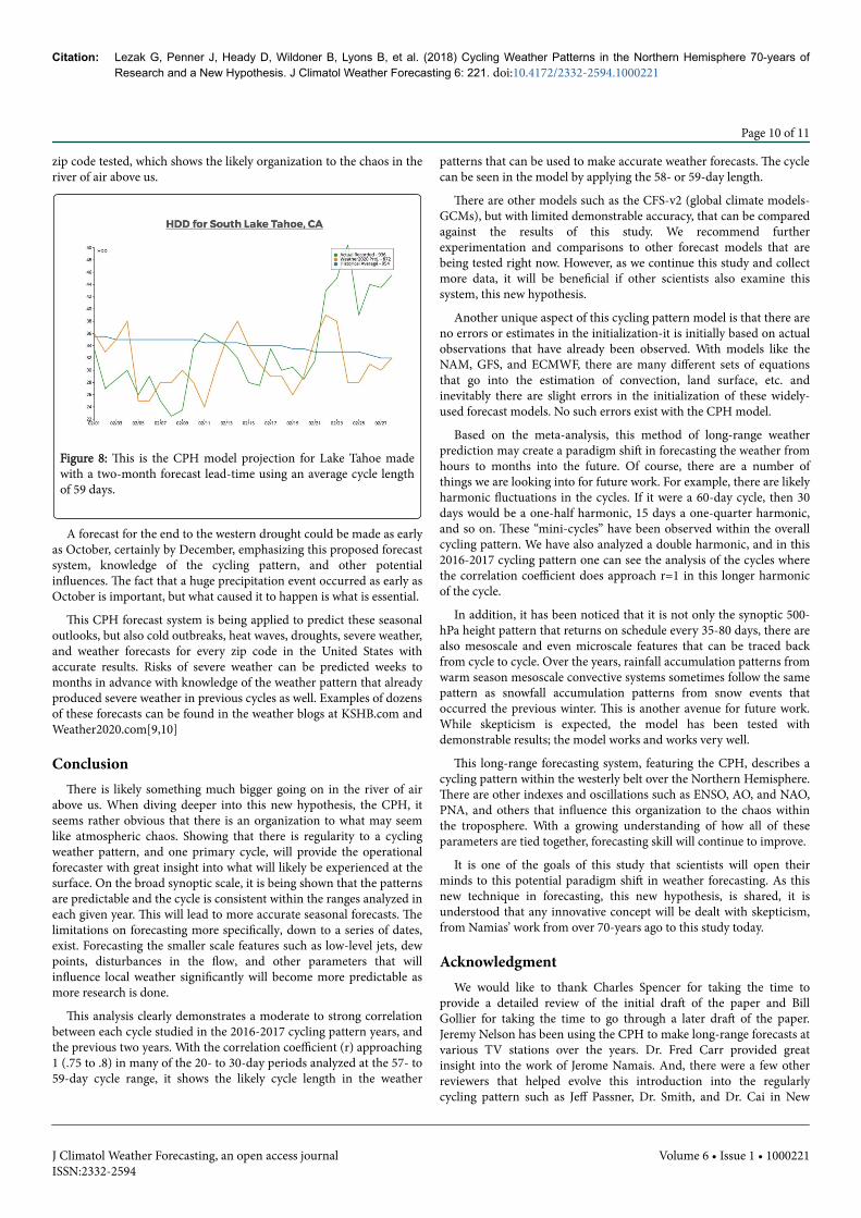
zip code tested, which shows the likely organization to the chaos in theriver of air above us.

Figure 8: This is the CPH model projection for Lake Tahoe madewith a two-month forecast lead-time using an average cycle lengthof 59 days.

A forecast for the end to the western drought could be made as earlyas October, certainly by December, emphasizing this proposed forecastsystem, knowledge of the cycling pattern, and other potentialinfluences. The fact that a huge precipitation event occurred as early asOctober is important, but what caused it to happen is what is essential.

This CPH forecast system is being applied to predict these seasonaloutlooks, but also cold outbreaks, heat waves, droughts, severe weather,and weather forecasts for every zip code in the United States withaccurate results. Risks of severe weather can be predicted weeks tomonths in advance with knowledge of the weather pattern that alreadyproduced severe weather in previous cycles as well. Examples of dozensof these forecasts can be found in the weather blogs at KSHB.com andWeather2020.com[9,10]

ConclusionThere is likely something much bigger going on in the river of air

above us. When diving deeper into this new hypothesis, the CPH, itseems rather obvious that there is an organization to what may seemlike atmospheric chaos. Showing that there is regularity to a cyclingweather pattern, and one primary cycle, will provide the operationalforecaster with great insight into what will likely be experienced at thesurface. On the broad synoptic scale, it is being shown that the patternsare predictable and the cycle is consistent within the ranges analyzed ineach given year. This will lead to more accurate seasonal forecasts. Thelimitations on forecasting more specifically, down to a series of dates,exist. Forecasting the smaller scale features such as low-level jets, dewpoints, disturbances in the flow, and other parameters that willinfluence local weather significantly will become more predictable asmore research is done.

This analysis clearly demonstrates a moderate to strong correlationbetween each cycle studied in the 2016-2017 cycling pattern years, andthe previous two years. With the correlation coefficient (r) approaching1 (.75 to .8) in many of the 20- to 30-day periods analyzed at the 57- to59-day cycle range, it shows the likely cycle length in the weather

patterns that can be used to make accurate weather forecasts. The cyclecan be seen in the model by applying the 58- or 59-day length.

There are other models such as the CFS-v2 (global climate models-GCMs), but with limited demonstrable accuracy, that can be comparedagainst the results of this study. We recommend furtherexperimentation and comparisons to other forecast models that arebeing tested right now. However, as we continue this study and collectmore data, it will be beneficial if other scientists also examine thissystem, this new hypothesis.

Another unique aspect of this cycling pattern model is that there areno errors or estimates in the initialization-it is initially based on actualobservations that have already been observed. With models like theNAM, GFS, and ECMWF, there are many different sets of equationsthat go into the estimation of convection, land surface, etc. andinevitably there are slight errors in the initialization of these widely-used forecast models. No such errors exist with the CPH model.

Based on the meta-analysis, this method of long-range weatherprediction may create a paradigm shift in forecasting the weather fromhours to months into the future. Of course, there are a number ofthings we are looking into for future work. For example, there are likelyharmonic fluctuations in the cycles. If it were a 60-day cycle, then 30days would be a one-half harmonic, 15 days a one-quarter harmonic,and so on. These “mini-cycles” have been observed within the overallcycling pattern. We have also analyzed a double harmonic, and in this2016-2017 cycling pattern one can see the analysis of the cycles wherethe correlation coefficient does approach r=1 in this longer harmonicof the cycle.

In addition, it has been noticed that it is not only the synoptic 500-hPa height pattern that returns on schedule every 35-80 days, there arealso mesoscale and even microscale features that can be traced backfrom cycle to cycle. Over the years, rainfall accumulation patterns fromwarm season mesoscale convective systems sometimes follow the samepattern as snowfall accumulation patterns from snow events thatoccurred the previous winter. This is another avenue for future work.While skepticism is expected, the model has been tested withdemonstrable results; the model works and works very well.

This long-range forecasting system, featuring the CPH, describes acycling pattern within the westerly belt over the Northern Hemisphere.There are other indexes and oscillations such as ENSO, AO, and NAO,PNA, and others that influence this organization to the chaos withinthe troposphere. With a growing understanding of how all of theseparameters are tied together, forecasting skill will continue to improve.

It is one of the goals of this study that scientists will open theirminds to this potential paradigm shift in weather forecasting. As thisnew technique in forecasting, this new hypothesis, is shared, it isunderstood that any innovative concept will be dealt with skepticism,from Namias’ work from over 70-years ago to this study today.

AcknowledgmentWe would like to thank Charles Spencer for taking the time to

provide a detailed review of the initial draft of the paper and BillGollier for taking the time to go through a later draft of the paper.Jeremy Nelson has been using the CPH to make long-range forecasts atvarious TV stations over the years. Dr. Fred Carr provided greatinsight into the work of Jerome Namais. And, there were a few otherreviewers that helped evolve this introduction into the regularlycycling pattern such as Jeff Passner, Dr. Smith, and Dr. Cai in New

Citation: Lezak G, Penner J, Heady D, Wildoner B, Lyons B, et al. (2018) Cycling Weather Patterns in the Northern Hemisphere 70-years ofResearch and a New Hypothesis. J Climatol Weather Forecasting 6: 221. doi:10.4172/2332-2594.1000221

Page 10 of 11

J Climatol Weather Forecasting, an open access journalISSN:2332-2594

Volume 6 • Issue 1 • 1000221

Mexico. And, Eswar Iyer helped tremendously with editing andrevising the final version of this study.

References1. Namias J (1950) The index cycle and its role in the general circulation. J

Meteor 7: 130-139.2. Namias J (1978) Multiple causes of the North American abnormal winter

1976-77. Mon. Wea. Rev 106: 279-295.3. Stern H, Davidson NE (2015) Trends in the skill of weather prediction at

lead times of 1–14 days. Quarterly Journal of the Royal MeteorologicalSociety 141: 2726-2736.

4. Novak DR, Bailey C, Brill KF, Burke P, Hogsett WA, et al. (2014)Precipitation and temperature forecast performance at the WeatherPrediction Center. Wea. Forecasting 29: 489-504.

5. Colucci SJ, Baumhefner DP (1992) Initial Weather Regimes as Predictorsof 30-Day Mean Forecast Accuracy. Wea Forecasting 49: 1652-1671.

6. Gensini VA, Marinaro A (2016) Tornado Frequency in the United StatesRelated to Global Relative Angular Momentum. Mo. Wea. Rev 144:801-810.

7. Madden RA, Julian PR (1971) Detection of a 40-50 day oscillation in thezonal wind in the tropical Pacific. J Atmos. Sci 28: 702-708.

8. Branstator G, Teng H (2017) Tropospheric Waveguide Teleconnectionsand Their Seasonality. J Atmos. Sci 74: 1513-1532.

9. Teng H, Branstator G (2017) Causes of Extreme Ridges that InduceCalifornia Droughts. J. Climate 30: 1477-1492.

10. Gershunov A, Shulgina T, Ralph FM, Lavers DA, Rutz JJ (2017) Assessingthe Climate-Scale Variability of Atmospheric Rivers affecting westernNorth America. Geophysical Research Letters 44: 7900-7908.

Citation: Lezak G, Penner J, Heady D, Wildoner B, Lyons B, et al. (2018) Cycling Weather Patterns in the Northern Hemisphere 70-years ofResearch and a New Hypothesis. J Climatol Weather Forecasting 6: 221. doi:10.4172/2332-2594.1000221

Page 11 of 11

J Climatol Weather Forecasting, an open access journalISSN:2332-2594

Volume 6 • Issue 1 • 1000221