Spatial Temporal Exponential-Family Point Process Modelsfor the Evolution of Social Systems

Joshua D. EmBree∗ Mark S. Handcock†

October 4, 2016

Abstract

We develop a class of exponential-family point processes based on a latent social space to model thecoevolution of social structure and behavior over time. Temporal dynamics are modeled as a discreteMarkov process specified through individual transition distributions for each actor in the system at agiven time. We prove that these distributions have an analytic closed form under certain conditions anduse the result to develop likelihood-based inference. We provide a computational framework to enableboth simulation and inference in practice. Finally, we demonstrate the value of these models by analyzingalcohol and drug use over time in the context of adolescent friendship networks.

Keywords: STEPP, social network analysis, spatial-temporal, point process, longitudinal, latent space,Markov, substance use.

1 Introduction

Social systems play a fundamental role in the dynamics of human behavior and interest in studying thesesystems is growing. For example, Fujimoto and Valente (2012) investigate contagion mechanisms for thetransmission of drinking and smoking behaviors through adolescent social networks. However, work ofthis nature is often limited by a lack of realistic stochastic models for the phenomena of interest. For suchmodels to be applicable, they must adequately represent the complexity of social relations and behavior asthey coevolve over time.

Most often, social relations are measured with dyadic tie variables, for example friendship, and thenassembled to form networks. There are numerous stochastic models for the evolution of social networks.Holland and Leinhardt (1977) provide one of the earliest continuous-time Markov models for the process bywhich social structure affects individual behavior. Arguably, the most popular subclass of these continuous-time Markov models is the so called stochastic actor-oriented model (SOAM) described in Snijders (2005) andSnijders, Van de Bunt, and Steglich (2010) which are framed in the context of individual actors makingdecisions to form or break ties with other actors. Snijders, Steglich, and Schweinberger (2007) extend theSAOMs to jointly model selection (individuals’ network-related choices) and influence (effect of actors oneach other’s attributes). The SAOM’s are accessible for practitioners through the RSiena (Ripley, Boitmanis,and Snijders, 2013) software package.

In addition to the continuous-time Markov models, exponential-family random graph models (ERGMs)provide a uniquely different view of social networks. Holland and Leinhardt (1981) introduce the first

∗Adjunct Researcher, RAND Corporation, Santa Monica, CA 90401 (E-mail: jembree@rand.org).†Professor of Statistics, Department of Statistics, University of California, Los Angeles, CA 90095-1554 (E-mail: handcock@ucla.edu).

arX

iv:1

610.

0004

8v1

[st

at.O

T]

30

Sep

2016

exponential-family of probability distributions for directed graphs which are applicable only to cross-sectional social networks. However, Robins and Pattison (2001) naturally extend this framework by al-lowing for dependence between graphs across discrete time steps. Moreover, Hanneke, Fu, Xing, et al.(2010) define a discrete Temporal ERGM (TERGM) which assumes an exponential-family model for the tran-sitions between graphs. Krivitsky and Handcock (2013) further specify TERGMs with the Separable TemporalERGM (STERGM) by postulating that the processes by which actors form and dissolve ties are independentor separable conditional on the previous state of the network. Various other discrete-time models for socialnetwork dynamics provide means for data driven analyses of social systems but drawbacks persist.

Observed social networks are typically represented by directed (or undirected) graphs where edges in-dicate the presence of a relationship, e.g., friendship. As a result, complex relations are reduced to a binaryindicator. Advances in latent space models for rank data (Gormley and Murphy, 2007) provide new contextfor conceptualizing this information. Hoff, Raftery, and Handcock (2002) summarize general latent spaceapproaches to social network analysis while Handcock, Raftery, and Tantrum (2007) describe an unob-served Euclidean social space where the actors’ locations arise stochastically from a mixture of distributionscorresponding to different clusters. These strategies are appealing for their flexibility and interpretabilitybut have only been developed for cross-sectional networks.

Since latent space approaches to social network analysis postulate the existence of an unobserved spacewhere points represent actors, a natural extension would be to propose a spatial-temporal point processfor the underlying dynamics. A major drawback in the current models for social network evolution is theassumption that the set of actors remains fixed over time. In real social systems, e.g., an urban high school,the set of actors is constantly changing so this assumption can be problematic. Spatial birth-death processes(Moller and Waagepetersen, 2003) offer a stochastic framework for the positions of actors as they enteror exit the system over time. Unfortunately, these process cannot model changes in persistent (present atseveral consecutive time points) actors’ positions. Hence, we seek a stochastic model that can reasonablydescribe the positions of actors as they enter, navigate, and exit the social space.

In Section 2, we formally define the social space and derive a discrete-time Markov process to describefundamental social phenomena. In Section 3, we present analytic results, develop likelihood-based inferen-tial methods, and discuss computation. In Section 4, we apply the methodology to a longitudinal study ofadolescent students to explore changes in risky behavior in the context of friendship networks. In Section5, we discuss the relevance of this work in broader social science research and consider extensions to themodeling framework.

2 Point Process Models for Social Systems

2.1 Conceptualization

To conceptualize the methods presented here, consider the population of people in a fixed location overtime, e.g., students at an urban middle school. We want to understand the social and behavior dynamicsof these people over time. For example, we might ask how a student’s social ties affect her propensity todrink alcohol or engage in risky sex. To do so, we need a rich representation of the time sensitive sociallandscape. Note that this approach is distinctly different from a traditional panel survey where we attemptto follow a fixed cohort over time. Instead, we focus on the interactions of a dynamic population in a fixedlocation where we may observe significant composition change within the group between waves of datacollection. That is, we do not expect to observe the same set of people at every wave.

Generally, consider a set of actors in social space at time t. In the example above, the actors are studentsand the social space is the school where they interact. Also consider the positions of actors in social spaceat time t. While we formalize this below, the intuition is straightforward: the set of distances betweenpositions in social space represent social relations. For example, two people who have been friends foryears tend to be very close to one another in the space whereas casual acquaintances tend to be considerablyfurther apart.

The major advantage of this conceptualization is flexibility. Complex and nuanced relationships can be

1

accurately represented by a distance metric. Conventionally, we study social networks where relationshipsare binary, e.g., 1 indicates a friendship nomination and 0 the absence of such a nomination.

2.2 Specification

For t = 0, 1, . . . , let N t = {1, . . . , nt} be the set of unique actor labels up to time t with N0 ⊆ N1 ⊆· · · and let St ⊆ N t denote the set of actors present at time t. Further, let (S , ‖·‖) be a normed spacewhere Zt = {Zti ∈ S : i ∈ St} is the set of actor locations at time t and Xt is an nt × q matrix of actorcovariates. We say that {St, Xt, Zt}t≥0 defines a social space. Next, suppose that St (and implicitly N t), Xt,and Zt are random variables that jointly form a stochastic process. If {St, Xt, Zt}t≥0 satisfies the Markovproperty in time and the transition probability P (St, Xt, Zt|St−1, Xt−1, Zt−1) is an exponential family, thenwe call {St, Xt, Zt}t≥0 a Spatial Temporal Exponential-Family Point Process (STEPP). Next, we construct afundamental class of STEPPs by making a few assumptions about the social space and deriving transitiondistributions.

Assumption 1: {St}t≥0 is a process exogenous to (Xt, Zt). Recall, St is the set of actors who are cur-rently in the system at time t, e.g., students in a classroom. While one can imagine many scenarios in whichthe actors who enter or exit the social space is endogenous, e.g., delinquent students are more likely to beexpelled, we focus here on the exogenous cases.

Assumption 2: Actor positions in social space, {Zti : i ∈ St}, are conditionally independent given theprevious positions, Zt−1. This assumes that actors move through the social space based on the informationavailable at the current time.

Assumption 1 makes modeling the composition change of actor sets between waves distinctly separatefrom the changes in actor positions and their corresponding covariates. We refer to {St}t≥0 as a migrationprocess where the actors who enter the system are immigrants and the actors who exit the system are emi-grants. Assumption 2 implies that we can marginalize the transition distributions at the actor-level. Thus,we derive a general class of STEPPs below by specifying the form of

P (Zti , Xti |Zt−1, Xt−1, St−1)

where it is implicit that i ∈ St. We refer to this as the ego transition distribution (ETD) and it is specifiedby a series of increasingly complex processes. These processes are basic drift, atomic drift, homophilousattraction, homophilous repulsion, heterophilous attraction, and heterophilous repulsion.

A basic drift process describes actor positions only and is determined by a single parameter δ0 ≥ 0. TheETD is given by

Pδ0(Zti |Zt−1, St−1) =exp

(−δ0

∥∥Zti − Zt−1i

∥∥)c(δ0)

(1)

wherec(δ0) =

∫S

exp(−δ0

∥∥z − Zt−1i

∥∥) · µ(dz)

is the normalizing constant. Note that given the space (S , ‖·‖), the underlying measure µ must be chosento ensure c(δ0) <∞. A basic drift process is the simplest stochastic model for actor mobility in social space.Along these lines, we also have behavior persistence. For m = 1, . . . , q and for every i ∈ St−1 ∩ St, let

ρm = P (Xtim = x|Xt−1

im = x) (2)

denote the probability that behavior m persists through a single transition. Note that this alone does notcompletely specify a probability distribution except in the case of a Bernoulli random variable. Also, notethat in the case where a covariate is structurally non-random, we can set ρm = 1.

To derive more complex processes, we need to formalize the notion of closeness in social space. For anyz ∈ S and k ∈ N, consider a set E ⊂ S with |E| <∞ and z /∈ E, where | · | denotes the counting measure.Let

I1 = arg minz′∈E

‖z − z′‖ .

2

For j = 2, . . . , k, let Jj−1 = E \⋃j−1l=1 Il where

Ij = arg minz′∈Jj−1

‖z − z′‖ .

Then we say that

Bk(z, E) =

k⋃j=1

Ij (3)

defines a neighbor set for z where E is the defining expression. Next, let w : S ×S → [0, 1] be a weightingfunction for two positions in social space. If w satisfies

(i) w(z, z) = 1;

(ii) there exists a z′ 6= z such that w(z, z′) = 1;

(iii) w(z, z′)→ 0 as ‖z − z′‖ → ∞;

(iv) w(z, z′)→ 0 as ‖z − z′‖ → 0.

then we say that it is an atomic weighting. For motivation of this definition, see Section 2.3 below.Similar to a basic drift process, an atomic drift process describes actor positions only and is determined

by a single parameter δ1 ≥ 0. However, the ETD is considerably more complex. For an atomic weightingw, atomic drift is defined by

Pδ1(Zti |Zt−1, St−1) =exp

(−δ1

∑j∈St−1 1(Zt−1

j ∈ Bk(Zt−1i , Zt−1

−i ))w(Zt−1i , Zt−1

j )∥∥Zti − Zt−1

j

∥∥)c(δ1)

(4)

where Zt−1−i = Zt−1 \ {Zt−1

i } and 1(·) is the indicator function. As specified above, Bk(Zt−1i , Zt−1

−i ) is, withsome exceptions, the set of k nearest neighbors of ego i at time t − 1. In the event that |St−1| ≤ k, thisneighbor set will have fewer than k members and in the event that multiple actors occupy the exact sameposition at t − 1, it could have more than k members. Nonetheless, we refer to this as the set of k nearestneighbors for ego i at time t − 1. Finally, we combine basic drift and atomic drift to define the general driftprocess which we denote

Pδ(Zti |Zt−1, St−1) = Pδ0(Zti |Zt−1, St−1)Pδ1(Zti |Zt−1, St−1)

Next, we introduce homophilous and heterophilous attraction processes. For a discrete covariate Xtm

and ego i, letAtim = {Zt−1

l ∈ Zt−1−i : l ∈ St−1, Xt

im = Xt−1lm }

andU tim = {Zt−1

l ∈ Zt−1−i : l ∈ St−1, Xt

im 6= Xt−1lm }.

Note that natural extensions exist for continuous covariates but we do not explicitly define them here. Forthe sake of this construction, assume that all covariates are discrete. Given a set of parameters α1, . . . , αq ≥ 0and an atomic weighting w, which we write wt−1

ij = w(Zt−1i , Zt−1

j ) for simplicity, the ETD of a homophilousattraction process on the mth covariate is

Pαm(Zti , X

ti |Zt−1, Xt−1, St−1) =

exp(−αm

∑j∈St−1 1(Zt−1

j ∈ Bk(Zt−1i , Atim))wt−1

ij

∥∥Zti − Zt−1j

∥∥)c(αm)

. (5)

3

The ETD for homophilous attraction on all covariates is defined by

Pα(Zti , Xti |Zt−1, Xt−1, St−1) =

q∏m=1

Pαm(Zti , X

ti |Zt−1, Xt−1, St−1) (6)

∝ exp

− q∑m=1

∑j∈St−1

αm1(Zt−1j ∈ Bk(Zt−1

i , Atim))wt−1ij

∥∥Zti − Zt−1j

∥∥ . (7)

Here, we omit the normalizing constant in the definition and use the proportional symbol, ∝. Given a setof parameters υ1, . . . , υq ≥ 0 and an atomic weighting w, the ETD of a heterophilous attraction process on themth covariate is

Pυm(Zti , Xti |Zt−1, Xt−1, St−1) =

exp(−υm

∑j∈St−1 1(Zt−1

j ∈ Bk(Zt−1i , U tim))wt−1

ij

∥∥Zti − Zt−1j

∥∥)c(υm)

, (8)

which is similar to homophilous attraction but with the neighbor set U tim. Naturally, the ETD for het-erophilous attraction on all covariates is defined by

Pυ(Zti , Xti |Zt−1, Xt−1, St−1) =

q∏m=1

Pυm(Zti , Xti |Zt−1, Xt−1, St−1) (9)

∝ exp

− q∑m=1

∑j∈St−1

υm1(Zt−1j ∈ Bk(Zt−1

i , U tim))wt−1ij

∥∥Zti − Zt−1j

∥∥ . (10)

Last, we introduce homophilous and heterophilous repulsion. If (S , ‖·‖) is a linear space, we can alterthe ETD for attraction to obtain an opposing effect which we refer to as repulsion. Given the determiningparameters α1, . . . , αq ≥ 0, the ETD of a homophilous repulsion process is given by

Pα(Zti , Xti |Zt−1, Xt−1, St−1) (11)

∝ exp

− q∑m=1

∑j∈St−1

αm1(Zt−1j ∈ Bk(Zt−1

i , Atim))wt−1ij

∥∥Zti − (2Zt−1i − Zt−1

j )∥∥ .

Note that repulsion-like distributions are possible in non-linear spaces but are not addressed here. Ho-mophilous repulsion is structurally very similar to homophilous attraction except we replace

∥∥Zti − Zt−1j

∥∥with

∥∥Zti − (2Zt−1i − Zt−1

j )∥∥ in the ETD. In a linear space, this has the effect of reflecting the point Zt−1

j

through Zt−1i and considering the attraction toward the reflected point which can be viewed as a repulsion

away from the original point Zt−1j . Similarly, for parameters υ1, . . . , υq , the ETD of a heterophilous repulsion

process is given by

Pυ(Zti , Xti |Zt−1, Xt−1, St−1) (12)

∝ exp

− q∑m=1

∑j∈St−1

υm1(Zt−1j ∈ Bk(Zt−1

i , U tim))wt−1ij

∥∥Zti − (2Zt−1i − Zt−1

j )∥∥ .

The complete specification for this class of STEPPs is a combination of the processes derived aboveand an exponential-family model for Pλ(St|St−1) where λ is a parameter vector that determines the dis-tribution. Recall that we assume an exogenous migration process which may take many forms, e.g., thenumber of emigrants follows a binomial distribution and the number of immigrants a Poisson distribution.To preserve generality, we do not further specify this distribution. For homophily (heterophily), either at-traction or repulsion can be used but not both simultaneously. Assuming homophilous and heterophilousattraction, we let

θ = (δ0, δ1, ρ1, . . . , ρq, α1, . . . , αq, υ1, . . . , υq, λ>)>

4

denote the complete parameter vector for this class of STEPPs. The complete transition probability is givenby

Pθ(St, Xt, Zt|St−1, Xt−1, Zt−1) = Pλ(St|St−1)

∏i∈St

Pδ(Zti |Zt−1, St−1) (13)

× exp

(q∑

m=1

1(Xtim = Xt−1

im ) log ρm + 1(Xtim 6= Xt−1

im ) log(1− ρm)

)(14)

× Pα(Zti , Xti |Zt−1, Xt−1, St−1)Pυ(Zti , X

ti |Zt−1, Xt−1, St−1), (15)

which is an exponential family. Although many other specifications exist for STEPPs, when we write(St, Xt, Zt) ∼ STEPP(θ) it is in reference to this particular class.

2.3 Description

In this section, we further describe and interpret the class of STEPPs constructed above. The previous sec-tion provides a formal specification. This section expands the intuition and motivation for each individualprocess as well as a complete view of the entire model class.

The drift processes should be regarded as foundational elements for this class of STEPPs. Basic driftis governed by δ0, a parameter that dictates the magnitude of actors’ movements between transitions, andhas the simplest ETD. The probability mass in the ETD is symmetric about the ego’s previous positionand the rate of decay is proportional to δ0. That is, larger values of δ0 place more mass near the previousposition than would smaller values. The mode of the ETD is always the ego’s previous position so basicdrift reinforces the notion that actors tend to navigate the social space with respect to their current positionrather than jump around sporadically. A STEPP with basic drift alone results in actors generally driftingaround the space making predictable, symmetric movements between transitions.

The ETD of atomic drift is considerably more complex than that of basic drift, but this is essential forensuring that a specification resembles actual social processes. In essence, the atomic drift process allowsother actors to impact the movement of the ego through a transition with the caveat that only a fixed numberof them may have an actual effect and their distance relative to the ego largely determines the magnitudeof said effect. We use neighbor sets to fix the number of actors in the social space who may have an effecton the ego because it’s impractical to assume that the ego is affected by every other actor at a given time.For example, if the social space is a large corporate office with thousands of employees, any one personcannot possibly know everyone else let alone be significantly influenced by them socially. It is more likelythat an employee is aware of a few hundred others and noticeably influenced by one or two dozen of them.Thus, we only sum over the k nearest neighbors in the atomic drift ETD. Focusing on the effect of a singleneighbor j on the ego i, the functional form would be

exp(−δ1w(Zt−1

i , Zt−1j )

∥∥Zti − Zt−1j

∥∥) .This is strikingly similar to the ETD for basic drift with the inclusion of a weight. This is where using atomicweights is crucial.

Newton’s law of universal gravitation tells us that any two bodies will attract one another with a forcethat is inversely proportional to the square of the distance between them. In particle physics, this forceis considered negligible due to the fact that individual atomic masses are extremely small in comparisonto surrounding bodies, e.g., the Earth. However, there is a repulsive electromagnetic force between twoatoms when the distance between them is small. This force exists due to the negative charge of the electronsassociated with each atom. One can imagine a universe where there are no large bodies to dwarf the mass ofindividual atoms so these forces can coexist. The observable result would be a weak attractive force betweenatoms that increases as the distance between them decreases. Once the distance becomes sufficiently small,there is a weak repulsive force that increases as the distance between the atoms decreases. Thus, a naturalbalance arises.

5

Schopenhauer (1974) cleverly describes this as the porcupine dilemma: “a number of porcupines huddledtogether for warmth on a cold day in winter; but, as they began to prick one another with their quills,they were obliged to disperse. However the cold drove them together again, when just the same thinghappened. At last, after many turns of huddling and dispersing, they discovered that they would be bestoff by remaining at a little distance from one another. In the same way the need of society drives the humanporcupines together, only to be mutually repelled by the many prickly and disagreeable qualities of theirnature.”

As such, we incorporate atomic weights in the ETD for an atomic drift process to provide general attrac-tion between actors while providing stability in the social space over time. In the complete ETD for atomicdrift, we combine the effects of each properly weighted neighbor and scale the overall effect by δ1. Intu-itively, the nearest neighbors have the largest effects and the furthest neighbors have the smallest effectsexcept in cases when near neighbors are too close to the ego. Recall that we only require atomic weights toapproach zero in the respective limits so the specific functional form may dramatically impact the dynamicsof a social space.

Homophilous and heterophilous attraction are similar to atomic drift but the primary difference is in thespecification of neighbor sets. In homophilous (heterophilous) attraction, the set Atim (U tim) is constructedbased on the random state of Xt

im which provides a crucial dependence between the ego’s social positionand behavior. Given the random state of Xt

im, we consider the set of nearest homophilous (heterophilous)neighbors based on the behavior of those neighbors at time t− 1 in order to compute the ETD. That is, theego does not speculate about the future behavior of others.

Homophilous (heterophilous) repulsion is similar to attraction since we use the same neighbor set Atim(U tim) in the ETD but the position adjustment is fundamentally different. Recall that for repulsion, we re-place

∥∥Zti − Zt−1j

∥∥with∥∥Zti − (2Zt−1

i − Zt−1j )

∥∥. In the ETD, the term∥∥Zti − Zt−1

j

∥∥ places some mass of thedistribution centered around the position of actor j at time t−1. It follows that the term

∥∥Zti − (2Zt−1i − Zt−1

j )∥∥

places the same mass centered around the position 2Zt−1i −Zt−1

j . In a linear space, this point is equivalent tothe reflection of Zt−1

j through Zt−1i . In this form, it is clear that repulsion is actually an opposing attraction.

In this model class, each process is straightforward and motivated by basic social forces. As a result,it may be difficult to grasp the gravity of a complete specification. Since we cannot include attraction andrepulsion on the same covariate, consider a STEPP with (basic and atomic) drift, homophilous attraction oneach covariate and heterophilous repulsion on each covariate. This complete process is extremely complexin its raw functional form but at the core, the ETD has a summation over different effects from neighboringactors to the ego. Each effect is slightly different depending on time-sensitive information (relative distancesbetween actors and behavior) and global properties determined by each parameter. By construction, eachparameter is non-negative so we can focus on their relative differences for interpretation. For example, thelargest of α1, . . . , αq indicates the covariate which exhibits the strongest attraction between similar actors.Alternatively, one of the υ1, . . . , υq being very small or 0 indicates a covariate which exhibits little to norepulsion between dissimilar actors. It is crucial to note that these parameters determine global propertiesof the social space as opposed to time dependent or individual properties which are the focus of futurework. Simulated examples of various STEPPs are available at http://tinyurl.com/STEPPMODELS.

3 Statistical Inference

3.1 Analysis for a general Euclidean social space

By slightly restricting the general STEPP model of Section 2, we can derive closed form ETDs and inferentialmethods. In this section, we show that the ETD for Zti conditional on Xt

i for any subset of the processesdescribed above is multivariate normal if S = Rd and the norm is Euclidean distance squared, i.e., ‖z‖ =∑di=1 z

2i . Based on this result, we derive the marginal ETD for Xt

i and provide a closed form distributionfor this class of STEPP models.

First, assume that S = Rd and for z ∈ S , ‖z‖ =∑di=1 z

2i . Using a general Euclidean space is somewhat

6

restrictive in a mathematical sense but practically, it provides a flexible, comprehensible foundation for thesocial space. From this point on, when we say ”distance” it is in reference to standard Euclidean distancewhereas the norm is specified above. To motivate using the square of Euclidean distance for a norm, weappeal to physics and the inverse square law which generally states

Intensity ∝ 1

distance2 .

In practice, we use the atomic weighting function

w(z1, z2) =

1 if z1 = z2

‖z1 − z2‖ if ‖z1 − z2‖ < c and z1 6= z2

‖z1 − z2‖−1 if ‖z1 − z2‖ ≥ c,

where 0 < c ≤ 1 is some threshold. Then when the distance between actors exceeds√c, the effect on the

ETD is inversely proportional to said distance squared. For shorter distances, we cannot apply the samerelationship because it leads to instability as previously discussed. Since many physical phenomena, e.g.,Newton’s law of universal gravitation, follow an inverse square law, it provides a natural foundation for aEuclidean social space. It is important to note that we need not specify an atomic weighting for the resultsin the section to hold, but it is necessary to properly motivate this specification.

Next, we will prove that the ETD has an analytic closed form through a series of lemmas leading up tothe final theorem. First, we adopt some notation. For functions h, g : Rd → R, if h(z) = g(z) + c0 where c0is a constant, we say h(z) � g(z).Lemma 1: For w1, . . . , wn ≥ 0 and µ1, . . . , µn ∈ Rd,

n∑j=1

wj ‖z − µj‖ � w∗ ‖z − µ∗/w∗‖

where

w∗ =

n∑j=1

wj and µ∗ =

n∑j=1

wjµj .

Proof. See the Supplementary Materials.

Lemma 2: Let Z ∈ Rd be a random vector with µ1, . . . , µn ∈ Rd, and w1, . . . , wn ≥ 0 where w∗ =∑ni=1 wi >

0 and µ∗ =∑ni=1 wiµi If P (Z = z) ∝ exp {−

∑ni=1 wi ‖z − µi‖}, then

Z ∼MVN(µ∗

w∗,

1

2w∗Id

).

Proof. See the Supplementary Materials.

Theorem: For each i ∈ St, [Zti |Xti , Z

t−1, Xt−1, St−1] ∼MVN (µti,Σti) where

µti =

∑j θ>Ht

ijwtijZ

t−1j∑

j θ>Ht

ijwtij

Σti =

(1

2∑j θ>Ht

ijwtij

)Id

and an explicit expression for the elements of Htij is given in the Supplementary Materials.

Proof. See the Supplementary Materials.

7

Since we assume that the covariates are discrete, it is straightforward to calculate the marginal distribu-tion of [Xt

i |Zt−1, Xt−1] based on the theorem. We know Pθ(Zti , X

ti |Zt−1, Xt−1) up to a normalizing constant

and Pθ(Zti , |Xt

i , Zt−1, Xt−1) completely so it is possible to integrate out Zti for each value of Xt

i . Since themarginal distribution of Zti is multivariate normal, this integral is a function of the variance Σti and thevalue of Xt

i . Then we know P (Xti |Zt−1, Xt−1) up to a normalizing constant for every value of Xt

i and canrenormalize these values to obtain the complete distribution. Thus, the complete ETD can be written inclosed form as

Pθ(Zti , X

ti |Zt−1, Xt−1) = Pθ(Z

ti |Xt

i , Zt−1, Xt−1)Pθ(X

ti |Zt−1, Xt−1).

Recall that the migration process {St}t≥0 is an exogenous exponential family so we have the necessarycomponents for a complete, closed form likelihood.

3.2 Likelihood-Based Inference

In this section, we use the analytic results from the previous section to develop a likelihood-based infer-ential framework. At this juncture, it is also possible to develop a full Bayesian inferential framework,however here we focus on a Frequentist inference framework. This provides straightforward calculationsof parameter estimates and standard errors that might otherwise be computational complex and conceptu-ally challenging to interpret. The natural extension to a full Bayesian framework will appear elsewhere.

Suppose that (St, Xt, Zt) ∼ STEPP(θ) for t = 0, . . . , τ . That is, this is one STEPP with τ transitions. Forbrevity, we suppress the superscripts and simply write (S,X,Z) to denote the complete data over all timesteps. Then the likelihood is given by

L(θ|S,X,Z) =

τ∏t=1

Pθ(St, Xt, Zt|St−1, Xt−1, Zt−1)

=

τ∏t=1

(∏i∈St

Pθ(Zti , X

ti |Zt−1, Xt−1, St)

)Pθ(S

t|St−1)

=

τ∏t=1

(∏i∈St

Pθ(Zti |Xt

i , Zt−1, Xt−1, St)Pθ(X

ti |Zt−1, Xt−1, St)

)Pθ(S

t|St−1).

It is implicit in this formulation that the initial state (S0, X0, Z0) is fixed and not random. It is natural toextend this model class to allow for a random initial state but it is not explored here. However, we mustnote that the parameters in this class of STEPPs determine transitions between states rather than isolatedstates so a model for (S0, X0, Z0) may be difficult to align conceptually.

As shown above, the likelihood function has a computationally closed form so we can use standard op-timization routines to obtain parameter estimates and standard errors. However, calculating the likelihoodcan be cumbersome due to the inherent complexity of each ETD. In the next section, we address these issuesand provide a general computational framework for performing likelihood-based inference.

3.3 Computation

In this section, we describe the computational challenges of implementing likelihood-based inference forSTEPP data. The likelihood function provided above is straightforward to calculate but doing so may becomputationally expensive. Since the migration process {St}t≥0 is exogenous, we focus on elements of thelikelihood that involve actor positions and covariates. Explicitly, we need to calculate

τ∏t=1

∏i∈St

Pθ(Zti |Xt

i , Zt−1, Xt−1, St)Pθ(X

ti |Zt−1, Xt−1, St).

As shown previously, [Zti |Xti , Z

t−1, Xt−1] follows a multivariate normal distribution so calculating

Pθ(Zti |Xt

i , Zt−1, Xt−1, St)

8

given parameters µti and Σti is extremely fast. However, calculating these parameters can be computation-ally demanding. For each time period t and ego i ∈ St, we must compute multiple pairwise distances,weights, neighbor sets and sum over every element. Above all, computing neighbor sets is the most de-manding. Given q covariates, a full specification requires computing up to 2q + 1 neighbor sets for eachego.

While we have shown that one can calculate the distribution of [Xti |Zt−1, Xt−1] for an arbitrary dis-

crete covariate, we focus on the case where the support of each is finite. Recall that Xti is a random vector

with q components and for each of them, we calculate every value in the probability mass function. Eachcalculation has a closed from but crucially depends on the variance Σti which is computationally demand-ing. Thus, we must calculate Σti conditional on each element in the full support of the vector Xt

i to obtainPθ(X

ti |Zt−1, Xt−1, St) as required.

In practice, we maximize the log likelihood function

`(θ) =

τ∑t=1

∑i∈St

logPθ(Zti |Xt

i , Zt−1, Xt−1, St) + logPθ(X

ti |Zt−1, Xt−1, St)

since it is slightly more stable numerically. Explicitly,

θ = arg maxθ∈Θ

`(θ)

is the maximum likelihood estimator.

3.4 Analysis

In this sub-section we consider the properties of the maximum likelihood estimator. The asymptotic prop-erties of the MLE will depend on the framework the inference is embedded in. If we could observe asequence of independent and identically distributed (IID) STEPPs, standard large sample theory wouldimply that θ is consistent and asymptotically efficient (Casella and Berger, 2002). Moreover, one can derivea standard Central Limit Theorem for this situation. However, in reality, we rarely can observe a sequenceof IID STEPPs since social systems are constantly evolving, and we do not detail analytic results pertainingto this case.

9

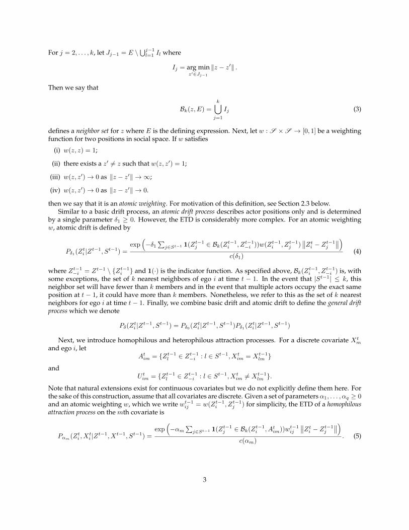
MLE Performance for Simulated STEPPs

Deviation from true parameter

-1 0 1

Basic Drift- δ0

Atmoic Drift- δ1

Homophilous Attraction- α1

Heterophilous Repulsion- υ1

Behavior Persistence- ρ1

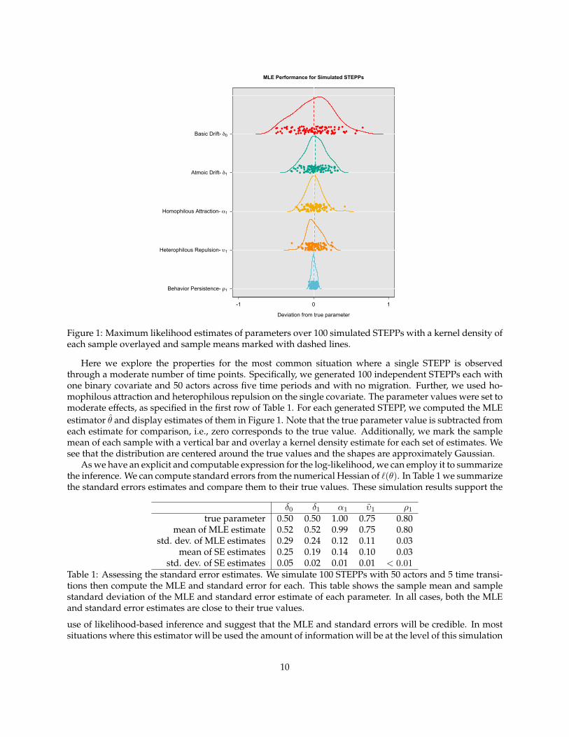
Figure 1: Maximum likelihood estimates of parameters over 100 simulated STEPPs with a kernel density ofeach sample overlayed and sample means marked with dashed lines.

Here we explore the properties for the most common situation where a single STEPP is observedthrough a moderate number of time points. Specifically, we generated 100 independent STEPPs each withone binary covariate and 50 actors across five time periods and with no migration. Further, we used ho-mophilous attraction and heterophilous repulsion on the single covariate. The parameter values were set tomoderate effects, as specified in the first row of Table 1. For each generated STEPP, we computed the MLEestimator θ and display estimates of them in Figure 1. Note that the true parameter value is subtracted fromeach estimate for comparison, i.e., zero corresponds to the true value. Additionally, we mark the samplemean of each sample with a vertical bar and overlay a kernel density estimate for each set of estimates. Wesee that the distribution are centered around the true values and the shapes are approximately Gaussian.

As we have an explicit and computable expression for the log-likelihood, we can employ it to summarizethe inference. We can compute standard errors from the numerical Hessian of `(θ). In Table 1 we summarizethe standard errors estimates and compare them to their true values. These simulation results support the

δ0 δ1 α1 υ1 ρ1

true parameter 0.50 0.50 1.00 0.75 0.80mean of MLE estimate 0.52 0.52 0.99 0.75 0.80

std. dev. of MLE estimates 0.29 0.24 0.12 0.11 0.03mean of SE estimates 0.25 0.19 0.14 0.10 0.03

std. dev. of SE estimates 0.05 0.02 0.01 0.01 < 0.01Table 1: Assessing the standard error estimates. We simulate 100 STEPPs with 50 actors and 5 time transi-tions then compute the MLE and standard error for each. This table shows the sample mean and samplestandard deviation of the MLE and standard error estimate of each parameter. In all cases, both the MLEand standard error estimates are close to their true values.

use of likelihood-based inference and suggest that the MLE and standard errors will be credible. In mostsituations where this estimator will be used the amount of information will be at the level of this simulation

10

or higher.The explicit form of the log-likelihood, `(θ), also make it possible to assess the goodness-of-fit of a

model via an analysis of deviance. Specifically, we can compute the change in log-likelihood from the nullmodel (θ = 0) to the MLE. Similarly, we can the graphical goodness-of-fit ideas to assess the overall fitof the model (Hunter, Goodreau, and Handcock, 2008a). To do so we can use temporal-structural networksummary statistics (e.g., persistence of ties, counts of nodal types) to compare observed behavior with thoseproduced by the STEPP model.

4 Application to Adolescent Risk Behavior in Networks

In this section we apply to a longitudinal network of friendships within a school. The primary question ofinterest is the coevolution of risky behavior and friendship ties. More specifically, the interaction betweensocial forces and substance use in adolescents has drawn significant attention in recent research. In par-ticular, researchers are interested in quantifying the effect of peers on individual behavior as well as theeffect an individual may have on their peers. Brechwald and Prinstein (2011) summarize recent advancesin the study of peer influence and explore the range of behaviors for which peer influence occurs. Poulin,Kiesner, Pedersen, and Dishion (2011) provide a longitudinal analysis of friendship selection on adoles-cent cigarette, alcohol, and marijuana use. Their analysis depends on a cross-lag panel model that testsfor the reciprocated association between substance use and the number of new friends who use the samesubstance. While this work provides unique insight into peer influence on adolescent substance use, thelack of sophisticated models for complex social processes is problematic.

The SAOMs discussed in section 1 have been applied by De La Haye, Green, Kennedy, Pollard, andTucker (2013) to explicitly model selection and influence in adolescent social networks with respect to mar-ijuana use at two schools in the Add Health study. Their results indicate that having friends who have usedmarijuana in their lifetime is not a significant predictor of individual initiation while recent (within the lastsix months) use is a significant predictor of individual initiation at one of the schools. Tucker, De La Haye,Kennedy, Green, and Pollard (2014) use SAOMs to model selection and influence effects of marijuana moreextensively in the Add Health study. They found that in one school, influence occurred in reciprocated re-lationships which are hypothesized to be characterized by closeness and trust. However, in another schoolit was found that adopting friends’ drug use behavior appears to be a strategy for attaining social status.SAOMs provide researchers with a sophisticated model for beginning to disentangle social forces and be-havior, but it requires strong assumptions. Specifically, the set of actors is assumed to remain fixed overtime and the coevolution of social structure and behavior is based on friendship tie variables which mayunstable.

4.1 CARBIN Study

The Contextualizing Adolescent Risk Behavior In Networks (CARBIN) study was designed to investigatechanges in risky behavior, e.g., drug use, amongst middle and high school students in the context of di-rected friendship networks. While several waves of data were collected from a few urban schools in Peoria,IL, we use four waves of data collected from one school for this illustration.

Each student student filled out an extensive survey that asked them about their personal behavior andto nominate their friends within the school. We utilize these friendship nominations to construct socialnetworks and focus on two substance use variables: any alcohol and any marijuana use in the last 30 days.Table 2 summarizes the raw data of interest for this exercise. Since there are only three time transitionsand the amount of composition change is relatively modest, we do not explore models for the migrationprocess. Instead, we focus on the latent social space and the processes that govern it. In the next section,we fit latent positions to the observed networks and estimate STEPP parameters.

11

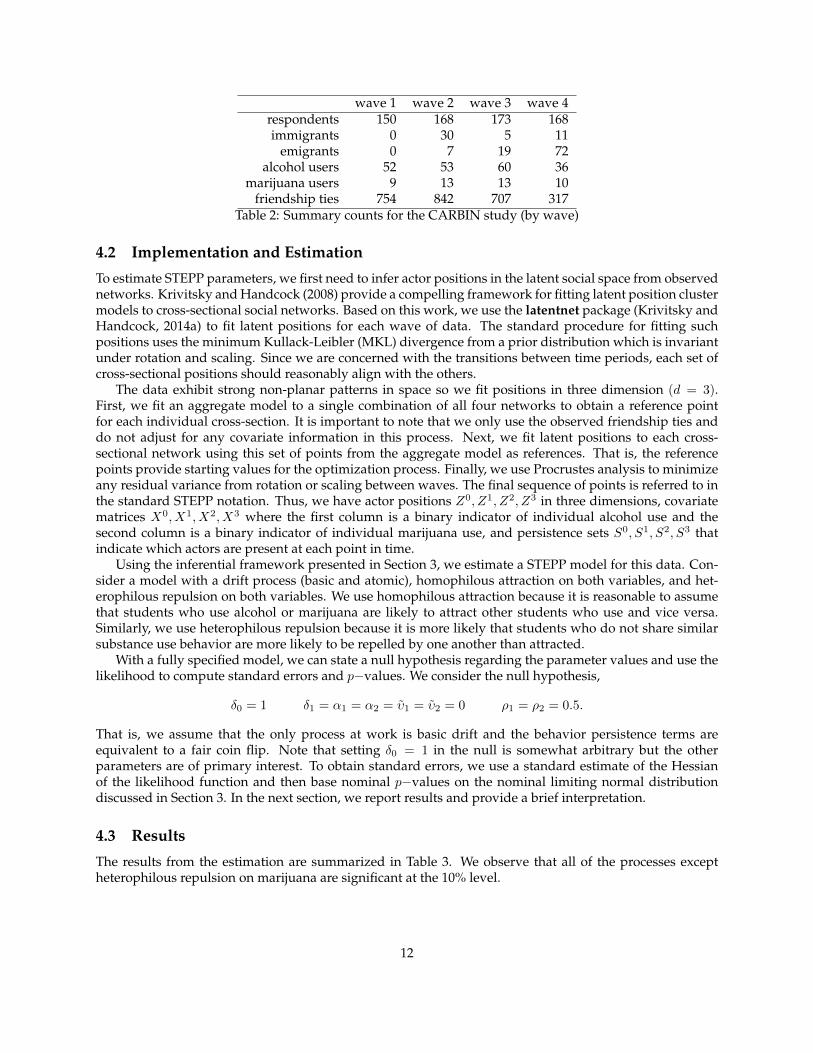
wave 1 wave 2 wave 3 wave 4respondents 150 168 173 168immigrants 0 30 5 11

emigrants 0 7 19 72alcohol users 52 53 60 36

marijuana users 9 13 13 10friendship ties 754 842 707 317

Table 2: Summary counts for the CARBIN study (by wave)

4.2 Implementation and Estimation

To estimate STEPP parameters, we first need to infer actor positions in the latent social space from observednetworks. Krivitsky and Handcock (2008) provide a compelling framework for fitting latent position clustermodels to cross-sectional social networks. Based on this work, we use the latentnet package (Krivitsky andHandcock, 2014a) to fit latent positions for each wave of data. The standard procedure for fitting suchpositions uses the minimum Kullack-Leibler (MKL) divergence from a prior distribution which is invariantunder rotation and scaling. Since we are concerned with the transitions between time periods, each set ofcross-sectional positions should reasonably align with the others.

The data exhibit strong non-planar patterns in space so we fit positions in three dimension (d = 3).First, we fit an aggregate model to a single combination of all four networks to obtain a reference pointfor each individual cross-section. It is important to note that we only use the observed friendship ties anddo not adjust for any covariate information in this process. Next, we fit latent positions to each cross-sectional network using this set of points from the aggregate model as references. That is, the referencepoints provide starting values for the optimization process. Finally, we use Procrustes analysis to minimizeany residual variance from rotation or scaling between waves. The final sequence of points is referred to inthe standard STEPP notation. Thus, we have actor positions Z0, Z1, Z2, Z3 in three dimensions, covariatematrices X0, X1, X2, X3 where the first column is a binary indicator of individual alcohol use and thesecond column is a binary indicator of individual marijuana use, and persistence sets S0, S1, S2, S3 thatindicate which actors are present at each point in time.

Using the inferential framework presented in Section 3, we estimate a STEPP model for this data. Con-sider a model with a drift process (basic and atomic), homophilous attraction on both variables, and het-erophilous repulsion on both variables. We use homophilous attraction because it is reasonable to assumethat students who use alcohol or marijuana are likely to attract other students who use and vice versa.Similarly, we use heterophilous repulsion because it is more likely that students who do not share similarsubstance use behavior are more likely to be repelled by one another than attracted.

With a fully specified model, we can state a null hypothesis regarding the parameter values and use thelikelihood to compute standard errors and p−values. We consider the null hypothesis,

δ0 = 1 δ1 = α1 = α2 = υ1 = υ2 = 0 ρ1 = ρ2 = 0.5.

That is, we assume that the only process at work is basic drift and the behavior persistence terms areequivalent to a fair coin flip. Note that setting δ0 = 1 in the null is somewhat arbitrary but the otherparameters are of primary interest. To obtain standard errors, we use a standard estimate of the Hessianof the likelihood function and then base nominal p−values on the nominal limiting normal distributiondiscussed in Section 3. In the next section, we report results and provide a brief interpretation.

4.3 Results

The results from the estimation are summarized in Table 3. We observe that all of the processes exceptheterophilous repulsion on marijuana are significant at the 10% level.

12

Parameter Estimate Std. Error p-valueBasic drift - δ0 0.0817 (0.018) < 0.0001∗∗∗

Atomic drift - δ1 0.0707 (0.041) 0.0873.Alcohol attraction - α1 0.0766 (0.027) 0.0053∗∗

Marijuana attraction - α2 0.0984 (0.042) 0.0181∗

Alcohol repulsion - υ1 0.1084 (0.018) < 0.0001∗∗∗

Marijuana repulsion - υ2 0.0000 (0.000) 0.9980Alcohol persistence - ρ1 0.7077 (0.024) < 0.0001∗∗∗

Alcohol persistence - ρ2 0.9248 (0.019) < 0.0001∗∗∗

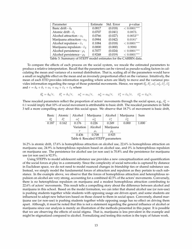
Table 3: Summary of STEPP model estimates for the CARBIN data.

To compare the effects of each process on the social system, we rescale the estimated parameters toproduce a relative interpretation. Recall that the parameters can be viewed as pseudo-scaling factors in cal-culating the mean and variance of a normal distribution. That is, scaling all of the parameters would havea small or negligible effect on the mean and an inversely proportional effect on the variance. Intuitively, themean of each ETD provides information regarding where actors are likely to move and the variance pro-vides information regarding the range of those potential movements. Hence, we report δ∗0 , δ∗1 , α∗1, α∗2, υ∗1 , υ∗2and τ = δ0 + δ1 + α1 + α2 + υ1 + υ2 where

δ∗0 = δ0/τ, δ∗1 = δ1/τ, α∗1 = α1/τ, α∗2 = α2/τ, υ∗1 = υ1/τ, υ∗2 = υ2/τ.

These rescaled parameters reflect the proportion of actors’ movements through the social space, e.g., δ∗0 =0.1 would imply that 10% of social movement is attributable to basic drift. The rescaled parameters in Table3 tell a more compelling story about this social space. We observe that 18.7% of movement is basic drift,

Basic Atomic Alcohol Marijuana Alcohol Marijuana Sumδ∗0 δ∗1 α∗1 α∗2 υ∗1 υ∗2

0.187 0.162 0.176 0.226 0.249 0.000 1.000Variation Alcohol Marijuana

τ ρ1 ρ2

0.436 0.708 0.925Table 4: Rescaled STEPP parameters

16.2% is atomic drift, 17.6% is homophilous attraction on alcohol use, 22.6% is homophilous attraction onmarijuana use, 24.9% is heterophilous repulsion based on alcohol use, and 0% is heterophilous repulsionon marijuana use. The persistence for alcohol use (or non use) is 70.8% and the persistence for marijuanause (or non use) is 92.5%.

Using STEPPs to model adolescent substance use provides a new conceptualization and quantificationof the social forces at play in a community. Since the complexity of social networks is captured by distancein Euclidean space, we do not need to model nuanced changes in friendship ties or shared substance use.Instead, we simply model the fundamental forces of attraction and repulsion as they pertain to each sub-stance. In the example above, we observe that the forces of homophilous attraction and heterophilous re-pulsion on alcohol are very strong, accounting for a combined 42.5% of the actors’ movements. Conversely,there is no heterophilous repulsion on marijuana and a modest homophilous attraction contributing to22.6% of actors’ movements. This result tells a compelling story about the difference between alcohol andmarijuana in this school. Based on the model formation, we can infer that shared alcohol use (or non-use)is pushing students together while students with opposing usage are driven apart, and some students areinfluenced to adopt new behaviors based on those closest to them in social space. Conversely, shared mar-ijuana use (or non-use) is pushing students together while opposing usage has no effect on driving themapart. Although, it must be noted that this is not a statement regarding the general influence of alcohol ormarijuana since our analysis is merely an illustration of the methods presented in this paper. It is possiblethat we are observing the effects of social stigma. That is, marijuana is less prevalent in the example andmight be stigmatized compared to alcohol. Formalizing and testing this notion is the topic of future work.

13

5 Discussion

This paper introduces a novel class of stochastic models for the coevolution of social structure and indi-vidual behavior over time. This model class is built on ideas successful applied in latent space approachesto network analysis, longitudinal social network analysis, and spatial-temporal point processes with spe-cific components being motivated by physics and psychology. Additionally, realistic specifications of thebroader class lead to traditional likelihood-based inference and computationally tractable solutions to esti-mation problems.

As shown in Section 2, complex social systems can be stochastically represented by a set of ego centricprocesses. The drift process provides an intuitive baseline for the ways in which actors navigate a socialspace with respect to their own position and neighboring actors’ positions. Moreover, the atomic driftprocess incorporates principles from particle physics to produce stable dynamics over time while Schopen-hauer’s porcupine dilemma provides a philosophical argument for the functional form of the transitiondistribution. The attraction and repulsion processes introduce a fundamental dependence between theevolution of individual behavior and one’s social position over time. That is, these processes shed lighton selection and influence phenomena in a way that is distinctly different from existing frames like theSAOMs.

While these models reflect real social processes, Section 3 shows that natural specifications also lead tomultivariate normal conditional ETDs and computationally tractable likelihood-based inference. It is easyto get lost in the technical details and lose sight of the overarching elegance in these results. Recall that weimplement a probabilistic version of the inverse square law, one of the most fundamental relationships innature, and the result is an analytically closed form transition distribution. Furthermore, that distribution isone of the most fundamental in science, nature and statistical theory: the multivariate normal distribution.Although the parameters of this distribution can be cumbersome to calculate, the result makes likelihood-based inference possible.

Section 4 illustrates the core methods developed in this paper with an application to a study of alcoholand drug use in adolescent friendship networks. This shows the potential of these methods in numerousapplications, but it also highlights future challenges. The process of fitting latent positions to cross-sectionalnetworks and minimizing the variation across observed points in time can be very nuanced and challeng-ing. It is not practical for applied researchers interested in implementing these models to perform thisexercise every time. Hence, the focus of future work in this area is to develop more holistic approachesto inferring latent actor positions. Alternatively, this class of models may lead to different forms of datacollection in social systems that inform the latent positions more accurately than social ties.

The STEPP framework for social systems can be extended both methodologically and in application. Inthis paper, we focus on population level forces but it is natural to extend the model to allow for individualor community level forces. A natural example is to extend the notion of attractive forces and allow actorsto have different masses. That is, some actors may have inherently more social influence or attractiveness.Also, we might allow for differential homophily or heterophily, e.g., the attractive force between non-usersis weaker than the force between users. In addition to methodological extensions, there are applications ofthe STEPP framework that do not require solving inferential problems. For example, one can use STEPPsimulation as a virtual laboratory for intervention assessment. Given reasonable assumptions regarding ac-tor positions and parameter values, it is possible to stage hypothetical interventions and simulate possibleoutcomes. Consider a class of 100 students where 40 of them are known binge drinkers and the administra-tion has two options: they can target a few students and conduct intense personal interventions that are 90%effective or implement a binge drinking prevention program that every student participates in but is only25% effective. Since targeting popular students could have spillover effects, it is unclear which option isbest. Furthermore, it is unclear which students to target. Simulated STEPPs shed light on an otherwise un-certain decision process. In conclusion, the STEPP framework provides realistic stochastic representationsof complex social systems which provides novel tools for social science research.

14

Acknowledgements

Research reported in this publication release was supported by the National Institute of Drug Abuse of theNational Institutes of Health under award number R01DA033280. The project described was supportedby grant numbers 1R21HD063000 and 5R21HD075714-02 from NICHD, grant number N00014-08-1-1015from the ONR, grant numbers MMS-0851555, MMS-1357619 from the NSF. We are grateful to the CaliforniaCenter for Population Research at UCLA (CCPR) for general support. CCPR receives population researchinfrastructure funding (R24-HD041022) from the Eunice Kennedy Shriver National Institute of Child Healthand Human Development (NICHD). Its contents are solely the responsibility of the authors and do not nec-essarily represent the official views of the Demographic & Behavioral Sciences (DBS) Branch, the NationalScience Foundation, the Office of Naval Research, or the National Institutes of Health. The authors wouldalso like to acknowledge Kayla de la Haye and the principal investigators of the CARBIN study, Harold D.Green, Jr. and Dorothy Espelage, for facilitating this work and motivating the methods presented in thispaper.

Appendix

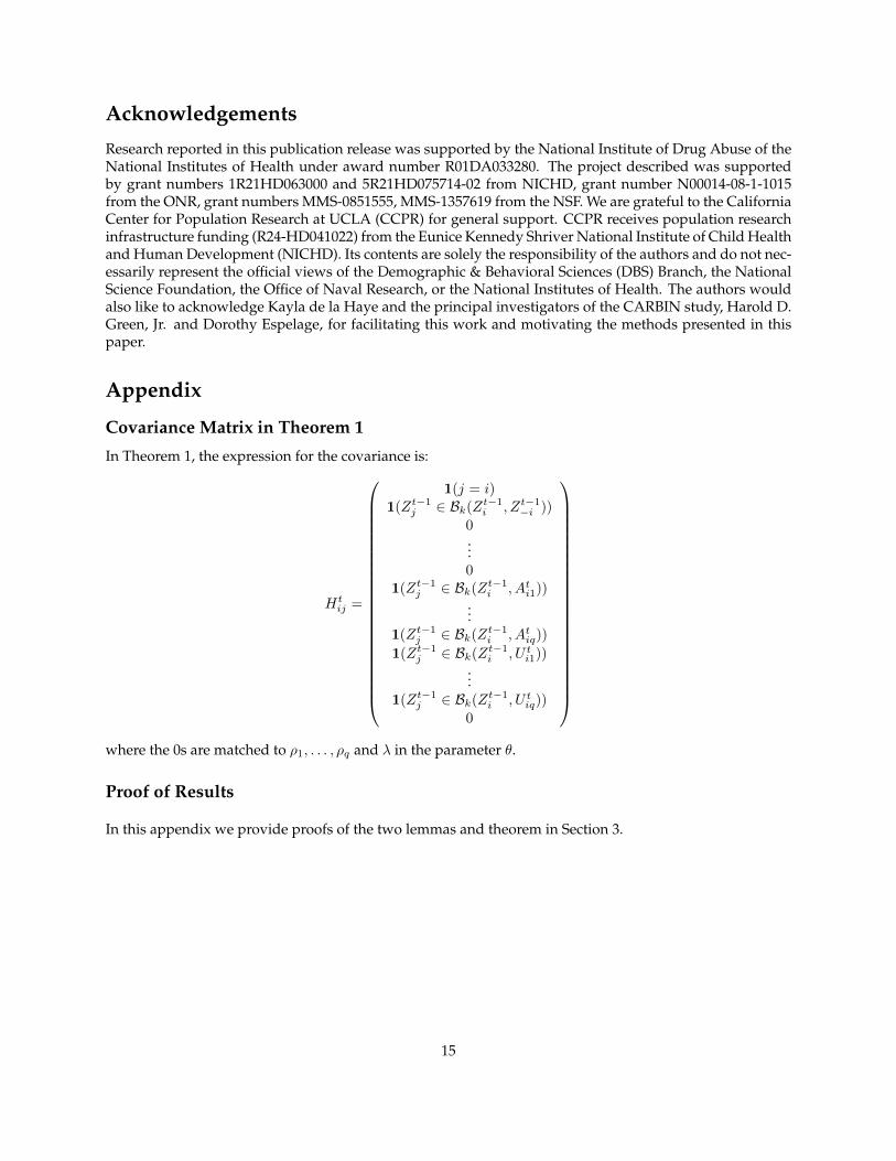
Covariance Matrix in Theorem 1

In Theorem 1, the expression for the covariance is:

Htij =

1(j = i)1(Zt−1

j ∈ Bk(Zt−1i , Zt−1

−i ))

0...0

1(Zt−1j ∈ Bk(Zt−1

i , Ati1))...

1(Zt−1j ∈ Bk(Zt−1

i , Atiq))

1(Zt−1j ∈ Bk(Zt−1

i , U ti1))...

1(Zt−1j ∈ Bk(Zt−1

i , U tiq))

0

where the 0s are matched to ρ1, . . . , ρq and λ in the parameter θ.

Proof of Results

In this appendix we provide proofs of the two lemmas and theorem in Section 3.

15

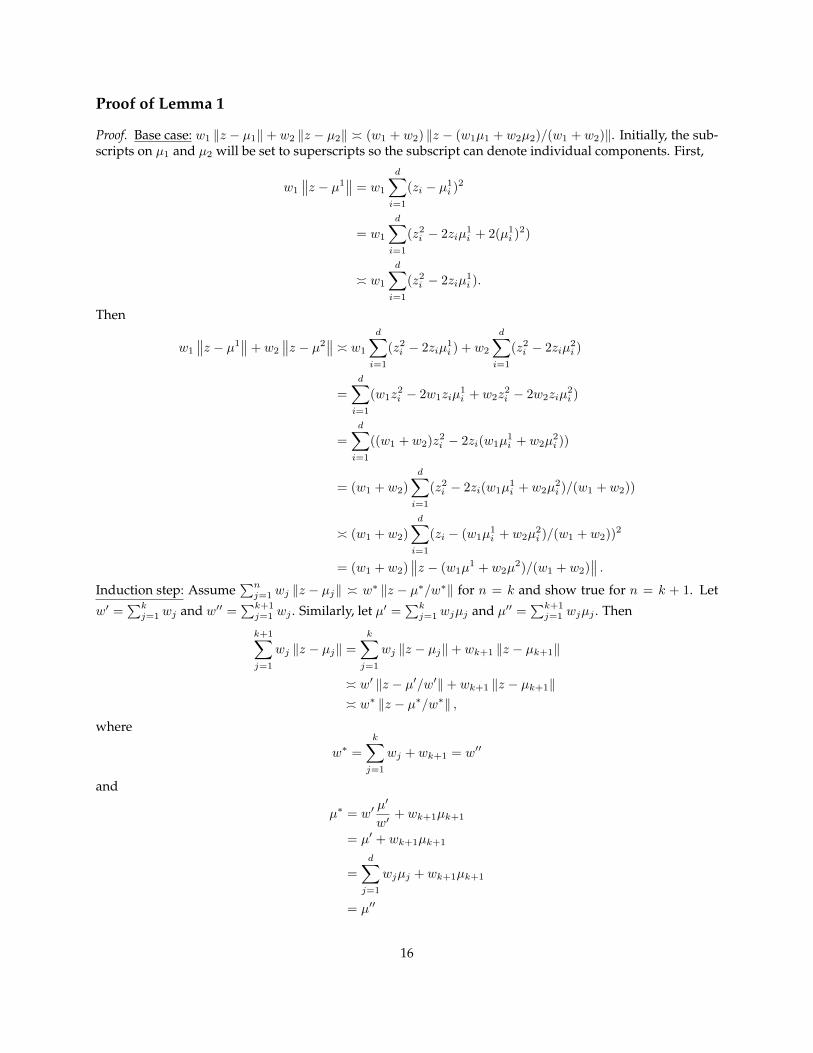
Proof of Lemma 1

Proof. Base case: w1 ‖z − µ1‖ + w2 ‖z − µ2‖ � (w1 + w2) ‖z − (w1µ1 + w2µ2)/(w1 + w2)‖. Initially, the sub-scripts on µ1 and µ2 will be set to superscripts so the subscript can denote individual components. First,

w1

∥∥z − µ1∥∥ = w1

d∑i=1

(zi − µ1i )

2

= w1

d∑i=1

(z2i − 2ziµ

1i + 2(µ1

i )2)

� w1

d∑i=1

(z2i − 2ziµ

1i ).

Then

w1

∥∥z − µ1∥∥+ w2

∥∥z − µ2∥∥ � w1

d∑i=1

(z2i − 2ziµ

1i ) + w2

d∑i=1

(z2i − 2ziµ

2i )

=

d∑i=1

(w1z2i − 2w1ziµ

1i + w2z

2i − 2w2ziµ

2i )

=

d∑i=1

((w1 + w2)z2i − 2zi(w1µ

1i + w2µ

2i ))

= (w1 + w2)

d∑i=1

(z2i − 2zi(w1µ

1i + w2µ

2i )/(w1 + w2))

� (w1 + w2)

d∑i=1

(zi − (w1µ1i + w2µ

2i )/(w1 + w2))2

= (w1 + w2)∥∥z − (w1µ

1 + w2µ2)/(w1 + w2)

∥∥ .Induction step: Assume

∑nj=1 wj ‖z − µj‖ � w∗ ‖z − µ∗/w∗‖ for n = k and show true for n = k + 1. Let

w′ =∑kj=1 wj and w′′ =

∑k+1j=1 wj . Similarly, let µ′ =

∑kj=1 wjµj and µ′′ =

∑k+1j=1 wjµj . Then

k+1∑j=1

wj ‖z − µj‖ =

k∑j=1

wj ‖z − µj‖+ wk+1 ‖z − µk+1‖

� w′ ‖z − µ′/w′‖+ wk+1 ‖z − µk+1‖� w∗ ‖z − µ∗/w∗‖ ,

where

w∗ =

k∑j=1

wj + wk+1 = w′′

and

µ∗ = w′µ′

w′+ wk+1µk+1

= µ′ + wk+1µk+1

=

d∑j=1

wjµj + wk+1µk+1

= µ′′

16

Proof of Lemma 2

Proof. First, observe that if h(z) � g(z), then eh(z) ∝ eg(z). Then by Lemma 1,

P (Z = z) ∝ exp

{−

n∑i=1

wi ‖z − µi‖

}

∝ exp

{−w∗

∥∥∥∥z − µ∗

w∗

∥∥∥∥} .Since we can rewrite ‖z‖ = z>z,

P (Z = z) ∝ exp

{−w∗

(z − µ∗

w∗

)>(z − µ∗

w∗

)}

= exp

{−1

2

(z − µ∗

w∗

)>(1

2w∗Id

)−1(z − µ∗

w∗

)}.

Therefore,

P (Z = z) = (2π)−d/2(2w∗)d/2 exp

{−1

2

(z − µ∗

w∗

)>(1

2w∗Id

)−1(z − µ∗

w∗

)}.

Proof of the Theorem

Proof. First, we need to verify the marginal distribution of [Zti |Xti , Z

t−1, Xt−1, St−1] up to a normalizingconstant. Recall the complete STEPP distribution

Pθ(St, Xt, Zt|St−1, Xt−1, Zt−1) = Pλ(St|St−1)

∏i∈St

Pδ(Zti |Zt−1, St−1)

× exp

(q∑

m=1

1(Xtim = Xt−1

im ) log ρm + 1(Xtim 6= Xt−1

im ) log(1− ρm)

)× Pα(Zti , X

ti |Zt−1, Xt−1, St−1)Pυ(Zti , X

ti |Zt−1, Xt−1, St−1).

By marginalizing and conditioning on St and Xti , we can reduce this to

P (Zti |Xti , Z

t−1, Xt−1) = Pδ(Zti |Zt−1, St−1)Pα(Zti , X

ti |Zt−1, Xt−1, St−1)Pυ(Zti , X

ti |Zt−1, Xt−1, St−1).

17

Since each term on the right hand side has an exponential form, the exponents sum as follows

δ0∥∥Zti − Zt−1

i

∥∥+ δ1∑j∈St

1(Zt−1j ∈ Bk(Zt−1

i , Zt−1−i ))wt−1

ij

∥∥Zti − Zt−1j

∥∥+

q∑m=1

∑j∈St

αm1(Zt−1j ∈ Bk(Zt−1

i , Atim))wt−1ij

∥∥Zti − Zt−1j

∥∥+

q∑m=1

∑j∈St

υm1(Zt−1j ∈ Bk(Zt−1

i , U tim))wt−1ij

∥∥Zti − Zt−1j

∥∥=∑j∈St

(δ01(i = j) + δ11(Zt−1j ∈ Bk(Zt−1

i , Zt−1−i )) +

q∑m=1

αm1(Zt−1j ∈ Bk(Zt−1

i , Atim))

+

q∑m=1

υm1(Zt−1j ∈ Bk(Zt−1

i , U tim)))wt−1ij

∥∥Zti − Zt−1j

∥∥=∑j∈St

θ>Htijw

tij

∥∥Zti − Zt−1j

∥∥ .Hence,

P (Zti |Xti , Z

t−1, Xt−1) ∝ exp

−∑j∈St

θ>Htijw

tij

∥∥Zti − Zt−1j

∥∥ .

and Lemma 2 implies that [Zti |Xti , Z

t−1, Xt−1, St−1] ∼MVN (µti,Σti).

References

Whitney A Brechwald and Mitchell J Prinstein. Beyond homophily: A decade of advances in understandingpeer influence processes. Journal of Research on Adolescence, 21(1):166–179, 2011.

G Casella and R. L. Berger. Statistical Inference. Duxbury, Pacific Grove, 2nd edition, 2002.

Kayla De La Haye, Harold D Green, David P Kennedy, Michael S Pollard, and Joan S Tucker. Selection andinfluence mechanisms associated with marijuana initiation and use in adolescent friendship networks.Journal of Research on Adolescence, 23(3):474–486, 2013.

Kayo Fujimoto and Thomas W Valente. Social network influences on adolescent substance use: Disentan-gling structural equivalence from cohesion. Social Science & Medicine, 74(12):1952–1960, 2012.

Isobel Claire Gormley and Thomas Brendan Murphy. A latent space model for rank data. In StatisticalNetwork Analysis: Models, Issues, and New Directions, pages 90–102. Springer, New York, 2007.

Mark S Handcock, Adrian E Raftery, and Jeremy M Tantrum. Model-based clustering for social networks.Journal of the Royal Statistical Society: Series A (Statistics in Society), 170(2):301–354, 2007.

Mark S. Handcock, David R. Hunter, Carter T. Butts, Steven M. Goodreau, Morris, and Martina. statnet:Software tools for the representation, visualization, analysis and simulation of network data. Journal ofStatistical Software, 24(1):1–11, 2008. URL http://www.jstatsoft.org/v24/i01.

Mark S. Handcock, David R. Hunter, Carter T. Butts, Steven M. Goodreau, Pavel N. Krivitsky, Skye Bender-deMoll, and Martina Morris. statnet: Software tools for the Statistical Analysis of Network Data. The StatnetProject (http://www.statnet.org), 2014a. URL CRAN.R-project.org/package=statnet. Rpackage version 2014.2.0.

18

Mark S. Handcock, David R. Hunter, Carter T. Butts, Steven M. Goodreau, Pavel N. Krivitsky, and MartinaMorris. ergm: Fit, Simulate and Diagnose Exponential-Family Models for Networks. The Statnet Project (http://www.statnet.org), 2014b. URL CRAN.R-project.org/package=ergm. R package version 3.1.2.

Steve Hanneke, Wenjie Fu, Eric P Xing, et al. Discrete temporal models of social networks. Electronic Journalof Statistics, 4:585–605, 2010.

Peter D Hoff. Bilinear mixed-effects models for dyadic data. Journal of the american Statistical association, 100(469):286–295, 2005.

Peter D Hoff, Adrian E Raftery, and Mark S Handcock. Latent space approaches to social network analysis.Journal of the american Statistical association, 97(460):1090–1098, 2002.

Paul W Holland and Samuel Leinhardt. Transitivity in structural models of small groups. ComparativeGroup Studies, 1971.

Paul W Holland and Samuel Leinhardt. A dynamic model for social networks. Journal of MathematicalSociology, 5(1):5–20, 1977.

Paul W Holland and Samuel Leinhardt. An exponential family of probability distributions for directedgraphs. Journal of the american Statistical association, 76(373):33–50, 1981.

David R. Hunter, Steven M. Goodreau, and Mark S. Handcock. Goodness of fit for social network models.Journal of the American Statistical Association, 103:248–258, 2008a.

David R Hunter, Mark S Handcock, Carter T Butts, Steven M Goodreau, and Martina Morris. ergm: A pack-age to fit, simulate and diagnose exponential-family models for networks. Journal of Statistical Software,24(3):nihpa54860, 2008b.

Pavel N Krivitsky and Mark S Handcock. Fitting position latent cluster models for social networks withlatentnet. Journal of Statistical Software, 24(2), 2008.

Pavel N Krivitsky and Mark S Handcock. A Separable Model for Dynamic Networks. Journal of the RoyalStatistical Sociey B, 75(4), 2013.

Pavel N. Krivitsky and Mark S. Handcock. latentnet: Latent position and cluster models for statistical networks.The Statnet Project (http://www.statnet.org), 2014a. URL CRAN.R-project.org/package=latentnet. R package version 2.5.1.

Pavel N. Krivitsky and Mark S. Handcock. tergm: Fit, Simulate and Diagnose Models for Network Evolutionbased on Exponential-Family Random Graph Models. The Statnet Project (http://www.statnet.org),2014b. URL CRAN.R-project.org/package=tergm. R package version 3.1.4.

Mark Lubell, John Scholz, Ramiro Berardo, and Garry Robins. Testing policy theory with statistical modelsof networks. Policy Studies Journal, 40(3):351–374, 2012.

Jesper Moller and Rasmus Plenge Waagepetersen. Statistical inference and simulation for spatial point processes.CRC Press, New York, 2003.

Martina Morris, Steven M Goodreau, Carter T Butts, Mark S Handcock, and David R Hunter. ergm: A pack-age to fit, simulate and diagnose exponential-family models for networks. Journal of Statistical Software,24(03), 2008.

Francois Poulin, Jeff Kiesner, Sara Pedersen, and Thomas J Dishion. A short-term longitudinal analysis offriendship selection on early adolescent substance use. Journal of adolescence, 34(2):249–256, 2011.

19

Ruth Ripley, Krists Boitmanis, and Tom A.B. Snijders. RSiena: Siena - Simulation Investigation for EmpiricalNetwork Analysis, 2013. URL http://CRAN.R-project.org/package=RSiena. R package version1.1-232.

Garry Robins and Philippa Pattison. Random graph models for temporal processes in social networks*.Journal of Mathematical Sociology, 25(1):5–41, 2001.

David R Schaefer, Sandra D Simpkins, Andrea E Vest, and Chara D Price. The contribution of extracur-ricular activities to adolescent friendships: New insights through social network analysis. Developmentalpsychology, 47(4):1141, 2011.

Arthur Schopenhauer. Parerga and paralipomena. short philosophical essays, vol. 2, translated by efj payne,1974.

Susan Shortreed, Mark S Handcock, and Peter Hoff. Positional estimation within a latent space model fornetworks. Methodology: European Journal of Research Methods for the Behavioral and Social Sciences, 2(1):24,2006.

Thomas A. B. Snijders, C. E. G. Steglich, and M. Schweinberger. Modeling the co-evolution of networksand behavior. In Kees van Montfort, Johan Oud, and Albert Satorra, editors, Longitudinal models in thebehavioral and related sciences, pages 41–71. Routledge, London, UK, 2007.

Tom AB Snijders. Models for longitudinal network data. Models and methods in social network analysis, 1:215–247, 2005.

Tom AB Snijders. Longitudinal methods of network analysis. Encyclopedia of complexity and system science,pages 5998–6013, 2009.

Tom AB Snijders, Gerhard G Van de Bunt, and Christian EG Steglich. Introduction to stochastic actor-basedmodels for network dynamics. Social networks, 32(1):44–60, 2010.

Christian Steglich, Tom AB Snijders, and Michael Pearson. Dynamic networks and behavior: Separatingselection from influence. Sociological Methodology, 40(1):329–393, 2010.

Joan S Tucker, Kayla De La Haye, David P Kennedy, Harold D Green, and Michael S Pollard. Peer influenceon marijuana use in different types of friendships. Journal of Adolescent Health, 54(1):67–73, 2014.

Gerhard G Van de Bunt, Marijtje AJ Van Duijn, and Tom AB Snijders. Friendship networks through time:An actor-oriented dynamic statistical network model. Computational & Mathematical Organization Theory,5(2):167–192, 1999.

20