josephson transistors interacting with dissipative...
TRANSCRIPT
JOSEPHSON TRANSISTORS INTERACTING
WITH DISSIPATIVE ENVIRONMENT
JUHA LEPPAKANGAS
Department of Physical Sciences
Division of Theoretical Physics
University of Oulu
Finland
Academic Dissertation to be presented with the assent of the Faculty ofScience, University of Oulu, for public discussion in the Auditorium L10, onApril 24th, 2009, at 12 o’clock noon.
REPORT SERIES IN PHYSICAL SCIENCES Report No. 53OULU 2009 • UNIVERSITY OF OULU
Opponent
Prof. Gerd Schon, Institut fur Theoretische Festkorperphysik,Universitat Karlsruhe, Germany
Reviewers
Prof. Stig Stenholm, Section of Laser Physics and Quantum optics,Royal Institute of Technology (KTH), Sweden
Ass. Prof. Goran Johansson, Applied Quantum Physics Laboratory,Chalmers University of Technology, Sweden
Custos
Prof. Erkki Thuneberg, Department of Physical Sciences,University of Oulu, Finland
ISBN 978-951-42-9093-0ISBN 978-951-42-9094-7 (PDF)ISSN 1239-4327OULU UNIVERSITY PRESSOULU 2009
i
Abstract
The quantum-mechanical effects typical for single atoms or molecules canbe reproduced in micrometer-scale electric devices. In these systems theessential component is a small Josephson junction (JJ) consisting of twosuperconductors separated by a thin insulator. The quantum phenomenacan be controlled in real time by external signals and have a great potentialfor novel applications. However, their fragility on uncontrolled disturbancecaused by typical nearby environments is a drawback for quantum informa-tion science, but a virtue for detector technology.
Motivated by this we have theoretically studied transistor kind of devicesbased on single-charge tunneling through small JJs. A common factor ofthe research is the analysis of the interplay between the coherent Cooper-pair (charge carriers in the superconducting state) tunneling and incoherentenvironmental processes. In the first work we calculate the current due toincoherent Cooper-pair tunneling through a voltage-biased small JJ in serieswith large JJs and compare the results with recent experiments. We are ableto reproduce the main experimental features and interpret these as tracesof energy levels and energy bands of the mesoscopic device. In the secondwork we analyze a similar circuit (asymmetric single-Cooper-pair transistor)but under the assumption that the Cooper-pair tunneling is mainly coher-ent. This predicts new resonant transport voltages in the circuit due tohigher-order processes. However, no clear traces of most of them are seenin the experiments, and similar discrepancy is present also in the case ofthe symmetric circuit. We continue to study this problem by modeling theinterplay between the coherent and incoherent processes more accuratelyusing a density-matrix approach. By this we are able to demonstrate that intypical conditions most of these resonances are indeed washed out by strongdecoherence caused by the environment. We also analyze the contributionof three typical weakly interacting dissipative environments: electromagneticenvironment, spurious charge fluctuators in the nearby insulating materials,and quasiparticles. In the last work we model the dynamics of a current-biased JJ perturbed by a smaller JJ using a similar density-matrix approach.We demonstrate that the small JJ can be used also as a detector of theenergy-band dynamics in a current biased JJ. The method is also used formodeling the charge transport in the Bloch-oscillating transistor.
Key words: Mesoscopic physics, Josephson junction, Cooper-pair tunneling,Decoherence

ii
Acknowledgments
This work was carried out in the Theoretical Physics Division, Departmentof Physical sciences, University of Oulu. I would like to thank the divisionleaders Prof. Erkki Thuneberg and Prof. Kari Rummukainen for arrangingthe facilities and helping me to get funding for this work. I thank Erkki, mysupervisor, for the patient and warm guidance during the different stages ofthe work. You are an easy person to approach with an impressive knowledgeand sense of physics. Also financial support from the Finnish Academy of Sci-ence and Letters, National Graduate School in Materials Physics, Universityof Oulu, and Academy of Finland are gratefully acknowledged.
I would like to express my gratitude to all the fellows in the Division,the past and the new ones, for the excellent atmosphere during the research!Especially Mikko Saarela, Pekka Pietilainen and Kirill Alexeev contributedto the work by stimulating discussions particularly in the seminar sessions.They always turned out to be fruitful for better understanding of the problem.Also Jani Tuorila, Timo Hyart, Timo Virtanen, Matti Silveri and JukkaIsohatala offered many enjoyable (off)scientific discussions and unforgettablemoments in the conference trips! Heikki Nykanen, Tauno Taipalemaki andKari Oikarinen are also gratefully acknowledged for their contribution.
I’ve been lucky to cooperate also with great experimentalists. I thankRene Lindell, Pertti Hakonen, Laura Korhonen and Antti Puska from theLow temperature Laboratory, Helsinki University of Technology, and YuriPashkin from the NEC, Japan, for giving me a change for a closer look intothe experimental part of the physics. The best moments during this workwere undoubtedly the ones when new experimental data were given to me,just waiting to be explored.
I’m in gratitude to my parents Arvo and Terttu, my sister Heli and mybrother-in-law Harri: your unlimited support and arrangement of numerousadventures in the wild Lapland are the basis of this accomplishment! Duringthe years I’ve learned that as important as it is to work with determinationand patience, it is to do something totally different. The local cycling com-munity has made this part to be even too easy! Finally, I do not forget myhigh-school teacher Juhani Janhonen who awoke my scientific curiosity.
Oulu, April 2009 Juha Leppakangas
iii
iv
LIST OF ORIGINAL PAPERS
The present thesis contains an introductory part and supplements to thefollowing papers which will be referred in the text by their Roman numbers.
I. J. Leppakangas, E. Thuneberg, R. Lindell, and P. Hakonen, Tunnel-
ing of Cooper pairs across asymmetric single-Cooper-pair transistors,Phys. Rev. B 74, 054504 (2006).
II. J. Leppakangas and E. Thuneberg, Coherent tunneling of Cooper pairs
in asymmetric single-Cooper-pair transistors, AIP Conference Proceed-ings 850, 947 (2006).
III. J. Leppakangas and E. Thuneberg, Effect of decoherence on resonant
Cooper-pair tunneling in a voltage-biased single-Cooper-pair transistor,Phys. Rev. B 78, 144518 (2008).
IV. J. Leppakangas and E. Thuneberg, Energy-band dynamics in a current-
biased Josephson junction probed by incoherent Cooper-pair tunneling,J. Phys.: Conf. Ser. 150, 022050 (2009).
The author has had a central role in all the articles presented in the thesis.He has developed the theory and computational tools around the phenomena,done all the simulations, and written the initial drafts of the articles.
Contents
Acknowledgments ii
List of original papers iv
Contents v
1 Introduction 1
2 Basics of Josephson junctions 5
2.1 Josephson effect . . . . . . . . . . . . . . . . . . . . . . . . . . 52.1.1 Ambegaokar-Baratoff relation . . . . . . . . . . . . . . 7
2.2 Junction dynamics . . . . . . . . . . . . . . . . . . . . . . . . 72.3 Interference and tunability . . . . . . . . . . . . . . . . . . . . 82.4 Secondary macroscopic quantum effects . . . . . . . . . . . . . 10
2.4.1 Semiclassical limit . . . . . . . . . . . . . . . . . . . . 11
3 Dissipative quantum mechanics 13
3.1 Reduced equation of motion . . . . . . . . . . . . . . . . . . . 133.1.1 Expanding the time-evolution operator . . . . . . . . . 153.1.2 Route to the diagrammatic formulation . . . . . . . . . 153.1.3 Master equation . . . . . . . . . . . . . . . . . . . . . . 16
3.2 Environments . . . . . . . . . . . . . . . . . . . . . . . . . . . 193.2.1 Electromagnetic environment . . . . . . . . . . . . . . 193.2.2 Quasiparticles . . . . . . . . . . . . . . . . . . . . . . . 213.2.3 Charge fluctuators . . . . . . . . . . . . . . . . . . . . 24
3.3 Fluctuations in a linear system . . . . . . . . . . . . . . . . . 263.3.1 Fluctuation-dissipation theorem . . . . . . . . . . . . . 263.3.2 Incoherent Cooper-pair tunneling . . . . . . . . . . . . 28
4 Applications 29
4.1 Cooper-pair box . . . . . . . . . . . . . . . . . . . . . . . . . . 294.1.1 Energy-level probing . . . . . . . . . . . . . . . . . . . 31
4.2 Single-Cooper-pair transistor . . . . . . . . . . . . . . . . . . . 344.2.1 Resonant Cooper-pair tunneling . . . . . . . . . . . . . 36
v
vi CONTENTS
4.2.2 Corrections using the density-matrix-approach . . . . . 374.2.3 External oscillator . . . . . . . . . . . . . . . . . . . . 39
4.3 Current-biased Josephson junction . . . . . . . . . . . . . . . 404.3.1 Calculation scheme . . . . . . . . . . . . . . . . . . . . 424.3.2 Probing energy-band dynamics . . . . . . . . . . . . . 444.3.3 Model for the Bloch-oscillating transistor . . . . . . . . 49
5 Summary 53
Bibliography 55
Chapter 1
Introduction
An interesting new field has emerged in the condensed matter physics withinthe last three decades. With the aid of advanced experimental techniquesthe quantum-mechanical effects typical for single atoms or molecules are re-produced in systems consisting of microfabricated electric-circuit elements.A central element in these devices is a Josephson junction (JJ) consisting oftwo superconductors separated by a thin insulator. These artificial entitiescan be controlled in a real-time fashion by electrical signals. The responseof the device demonstrates quantum mechanics at appropriate conditions:sub-Kelvin temperatures and for micrometer-scale elements. This new fieldhas opened up a unique possibility for exploring, testing and implementingquantum effects in microscale systems. Because the devices are easily inte-grable to other electrical entities, the novel applications proposed have a greatpotential in replacing the traditional computer and detector technology [1].
The triumph of science in the last century was the revealing of the physicsthat controls the dynamics of single atoms, namely the quantum mechanics.In short terms, it describes using a rigorous mathematical language that thematter interacts as it would consist of particles and travels as it would consistof waves. The theory seemingly contradicts with our observations in theeveryday life, although it successfully explains the basic processes behind it.The true quantum mechanical properties, e.g., the wave nature of particles,are deep down in the condensed systems, but are directly detected only assmall-scale single-particle effects in laboratories. The quantum mechanics inmost cases reduces to the classical mechanics at the scale of the everyday life.But there are no fundamental obstacles for realising the quantum world ata much larger scale. Indeed, also systems with nonclassical behaviour at themacroscopic scale exists. An example of such a system is a superconductor,whose ultimate conductivity is explained by a collective quantum-mechanicalstate, becoming possible at very low temperatures. This thesis considersresearch done on microscale Josephson devices in which also other type ofquantum effects can be brought a step closer to the scale of the everyday life.
1
2 CHAPTER 1. INTRODUCTION
The Josephson junction consists of two superconductors separated by athin insulator. If the insulating barrier between the superconductors is ofproper thickness, the collective quantum-mechanical state across the barrierresults in special current-voltage characteristics. The effect is very sensitiveto external influences, and its discovery about 50 years ago [2, 3] was fol-lowed by important applications in, for example, detection of weak magneticfields [4]. The JJ can be described, in the simplest form, as a fictitious clas-sical particle in a certain potential field. In the 1980s it was experimentallyverified that the JJ has also a wave nature: in proper conditions the fictitiousparticle is able to quantum-mechanically tunnel across its potential field, sud-denly switching the JJ to a different state [5, 6]. It was also shown that theenergy of this particle is quantized [7]. Further, in the 1990s, the real-timecontrollability of the populations of these quantum states was experimentallydemonstrated [8, 9]. Since then coupling to various other quantum systems,such as, nanoscale mechanical oscillators [10], photon cavities [11] and elec-tromagnetic oscillators [12] have been actively investigated largely due totheir great potential for nanotechnological applications. The most ambitioustask is probably the building of a solid-state quantum-computer using theJJs as the elementary components of its quantum bits [13, 14]. Such a devicewould start a new age in the computer technology, but is not a subject ofthe nearby future. Before that the knowledge of the relevant physics needsto be greatly improved by the basic research in the field.
These “secondary” macroscopic quantum effects are characteristic for mi-croscale JJs at low temperatures. The billions of particles involved suggeststhat the devices should be regarded macroscopic, but the length scale fallsinto the intermediate region between the macro and atomic worlds, namelyto the mesoscopic region. Still, the fact that a mesoscopic device, enormousin the atomic scale, can behave collectively as a controllable single atom ormolecule, is outstanding. Also, the nearby environment of such a device islarge but behaves rather undeterministically causing a lot of disturbance,called noise. The noise can originate in, e.g., the electric circuitry connectedto the system or in the nearby materials of the device. All the noise mecha-nisms in these devices are not clear yet. The quantum effects are very fragileto this kind of disturbance as they lead to loss of their “wave” coherence,to decoherence. Due to this the field aiming for processing information inquantum-mechanical states of the system has slightly lost ground, and is nowfighting against this problem [15]. Another subfield has seen this property asa possibility for probing the mesoscopic physics, the small JJs can be madeto work as excellent detectors of their environment [16, 17, 18, 19]. The workpresented in this thesis can be seen to fall in both of these subfields. Westudy the effect of decoherence on the quantum-mechanical evolution of thesystems that can be utilized whether in the quantum-information science orin the study of the mesoscopic physics.
3
The experimental study of macroscopic quantum systems in the last threedecades has also revived the theoretical field of quantum decoherence [20],already discussed in the early days of quantum mechanics. It considers a(quantum) system interacting with a large environment, the very problem ofthe applications. In this approach the average properties of the system seenby the environment are calculated by finding an approximative solution of theSchrodinger equation written for the whole system. The environment causesdecoherence when taking information out of the systems internal quantumevolution. Such a treatment is closely related to the fundamental idea ofquantum measurement, that measuring a state collapses the original state.The conscious experimentalist is here replaced by environment, still gatheringinformation out of the device. Indeed, the assumption that every interactioncan be described by a Schrodinger equation actually leads to the probabilisticoutcome of the process, as postulated in the usual interpretation of quantummechanics. So is there a difference between ordinary many particle processand the thing called quantum measurement? An irritating difference is thatin the former all the outcomes of the experiment occur, but do not interfere.In this picture the measurement causes only an appearance of the collapse:it does not occur but appears if looked in one of the possible lifelines. Theproblems of measurement, observation and sudden collapse still puzzle physi-cists but are now brought into new light as macroscopic quantum physics isa part of present-day experimental physics.
In this thesis we report theoretical studies done on transistor kind ofdevices build of small JJs. The operation of these Josephson transistors isbased on controlling single-Cooper-pair tunneling through the JJs. We havecalculated the current-voltage characteristics of the devices by simulatingthe dissipative quantum mechanics of the systems. The systems interactwith their nearby environment, mainly consisting of an electromagnetic en-vironment formed my the leads attached to the device, of spurious chargefluctuators in the nearby insulating materials, and of quasiparticles (unpairedelectrons). They all can have drastic effect on the characteristics of the de-vice, or the device can be based on their contribution. We study the interplaybetween coherent Cooper-pair tunneling and incoherent environmental pro-cesses using theoretical methods typical for problems dealing with quantumdecoherence. We compare the results with recent experiments and try toimprove the knowledge of the behaviour of such systems. We start in Chap-ter 2 by discussing the basic physics of Josephson junctions. In Chapter 3 weintroduce models for dissipative quantum mechanics and discuss the proper-ties of the relevant environments causing the dissipation. These chapters aremeant to be introductions to the subjects and do not contain any new results.In Chapter 4 we introduce the studied devices, present the main results ofPapers and extend some of the results. A summary is given in Chapter 5.

4 CHAPTER 1. INTRODUCTION
Chapter 2
Basics of Josephson junctions
The studies presented in this thesis consider characteristics of devices that arebased on the Josephson effect. The effect occurs between two superconduc-tors separated by a thin insulator. The superconducting state is that whatmakes the effect anomalous, as the collective quantum-mechanical groundstate extends across the barrier leading to special current-voltage (I − V )characteristics. The Josephson effect can be traced back to simple Josephsonrelations, but describing the behaviour of a more complicated many-bodysystem. At low temperatures and for small JJs the effect acquires a newcharacter as also “secondary” macroscopic quantum effects start to play animportant role.
2.1 Josephson effect
Superconductivity can be understood as a quantum-mechanical state thatextends to the macroscopic scale [21]. Despite their repulsive electric force,the conduction electrons in metal can have a small attractive net force dueto higher-order interaction with phonons, i.e., lattice vibrations. If such aninteraction exists, and the metal is cooled down so that the thermal energykBT is smaller than the pair binding energy ∆, the electrons form boundpairs, called the Cooper pairs [22, 4]. The pairs have no spin and behaveas bosons. The electrons are not tightly bound, as the size of the pair ismuch larger than the typical distance between two nearby electrons. How-ever, the pairs prefer the same quantum-mechanical state resulting in theultimate conductivity of superconductors. It follows that the state of sucha condensate can be described by the macroscopic wave function (of Cooperpairs)
Ψ(t, r) =√
ρ(t, r) exp[iθ(t, r)], (2.1)
where ρ(t, r) is proportional to the Cooper-pair density and the changes ofthe phase θ(t, r) can be related to the supercurrent.
5
6 CHAPTER 2. BASICS OF JOSEPHSON JUNCTIONS
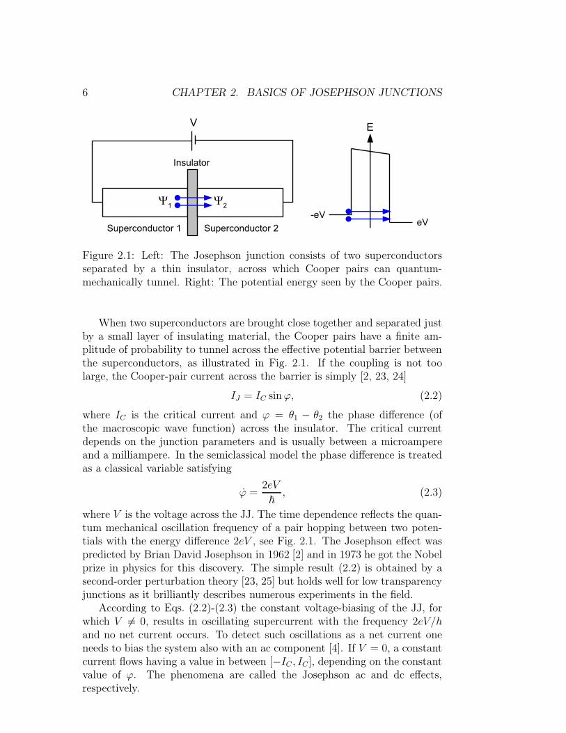
Figure 2.1: Left: The Josephson junction consists of two superconductorsseparated by a thin insulator, across which Cooper pairs can quantum-mechanically tunnel. Right: The potential energy seen by the Cooper pairs.
When two superconductors are brought close together and separated justby a small layer of insulating material, the Cooper pairs have a finite am-plitude of probability to tunnel across the effective potential barrier betweenthe superconductors, as illustrated in Fig. 2.1. If the coupling is not toolarge, the Cooper-pair current across the barrier is simply [2, 23, 24]
IJ = IC sinϕ, (2.2)
where IC is the critical current and ϕ = θ1 − θ2 the phase difference (ofthe macroscopic wave function) across the insulator. The critical currentdepends on the junction parameters and is usually between a microampereand a milliampere. In the semiclassical model the phase difference is treatedas a classical variable satisfying
ϕ =2eV
~, (2.3)
where V is the voltage across the JJ. The time dependence reflects the quan-tum mechanical oscillation frequency of a pair hopping between two poten-tials with the energy difference 2eV , see Fig. 2.1. The Josephson effect waspredicted by Brian David Josephson in 1962 [2] and in 1973 he got the Nobelprize in physics for this discovery. The simple result (2.2) is obtained by asecond-order perturbation theory [23, 25] but holds well for low transparencyjunctions as it brilliantly describes numerous experiments in the field.
According to Eqs. (2.2)-(2.3) the constant voltage-biasing of the JJ, forwhich V 6= 0, results in oscillating supercurrent with the frequency 2eV/hand no net current occurs. To detect such oscillations as a net current oneneeds to bias the system also with an ac component [4]. If V = 0, a constantcurrent flows having a value in between [−IC , IC], depending on the constantvalue of ϕ. The phenomena are called the Josephson ac and dc effects,respectively.
2.2. JUNCTION DYNAMICS 7
2.1.1 Ambegaokar-Baratoff relation
When the conductors are in the normal (not superconducting) state, thetunnel junction shows a resistive behaviour with an ohmic law I ≈ V/RT dueto electron tunneling through the barrier. As both the normal and Josephsoncurrent describe similar physics, they are not independent quantities. Forzero temperature (T = 0), which is a good approximation in the studiesconsidered, and general types of superconductors at different sides of the JJ,the so-called Ambegaokar-Baratoff relation [26] binds the critical current, thenormal state resistance RT and the superconducting energy gaps ∆i as
IC =∆1
eRTK
√
1 −(
∆1
∆2
)2
, (2.4)
where ∆1 is the smaller of the energy gaps and K(x) the complete ellipticintegral of the first kind. The elliptic integral satisfies K(0) = π/2 and is anincreasing function in the range considered. The nearby environment can alsoslightly contribute to this value [27]. Such corrections usually renormalize ICbut leave the functional dependence (2.2) unchanged.
2.2 Junction dynamics
The Josephson current is a ground state property and is dissipationless. TheJJ stores energy which can be calculated to be
EJ =
∫
dtIJV = −EJ cos(ϕ), (2.5)
where EJ = ~IC/2e is the Josephson coupling energy. The junction regionbehaves also capacitively as charge gathers on the edges of the superconduc-tors in the case of finite potential difference. The Coulomb energy of the JJwith capacitance C can be expressed as
EC =Q2
2C=
(CV )2
2C=C
2
(
~
2e
)2
ϕ2. (2.6)
The energies (2.5) and (2.6) can be interpreted as the potential and thekinetic energy, respectively, of a fictitious particle with mass C(~/2e)2. TheLagrangian treatment with such an identification leads to the Hamiltonianfunction
H =1
2C
(
2e
~
)2
p2 − EJ cos(ϕ), (2.7)
8 CHAPTER 2. BASICS OF JOSEPHSON JUNCTIONS
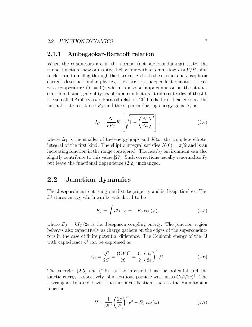
Figure 2.2: Left: The dynamical model for a JJ consists of parallel capacitorC, resistor R(V ) and supercurrent IJ . Center: The supercurrent can also beseen as a nonlinear inductor. Right: The equivalent schematic drawing usedin the thesis.
where p = (~/2e)Q is the conjugated variable of ϕ. The related Hamiltonianequations of motion describe the dissipationless dynamics of the JJ, i. e.,charging of the capacitor due to the Josephson current and the evolution ofthe phase difference due to charge in the capacitor.
The Josephson junction can also be treated as an inductance
L =V
IJ=
(
~
2e
)21
EJ cos(ϕ), (2.8)
in parallel with the capacitor C. Since the inductance is not a constant, itsresponse is nonlinear. This is an important property since the nonlinearityleads to nonconstant energy-level splitting, enabling the reduction of thesystem to two levels [24].
Also dissipative current can flow through the JJ via formation of quasi-particles, i. e., by breaking the Cooper pairs when eV > 2∆ [4]. This canbe modeled as a parallel resistor R(V ). In the language of the fictitiousparticle this means that there is a friction force entering the system after thethreshold velocity 4∆/~. The dynamical model of a Josephson junction isvisualized in Fig. 2.2.
2.3 Interference and tunability
In the presence of a magnetic field the Josephson effect acquires interestingproperties. The theory is as before, but the phase difference is replaced byits gauge invariant form
γ = ϕ− 2π
Φ0
∫
A · ds, (2.9)
2.3. INTERFERENCE AND TUNABILITY 9
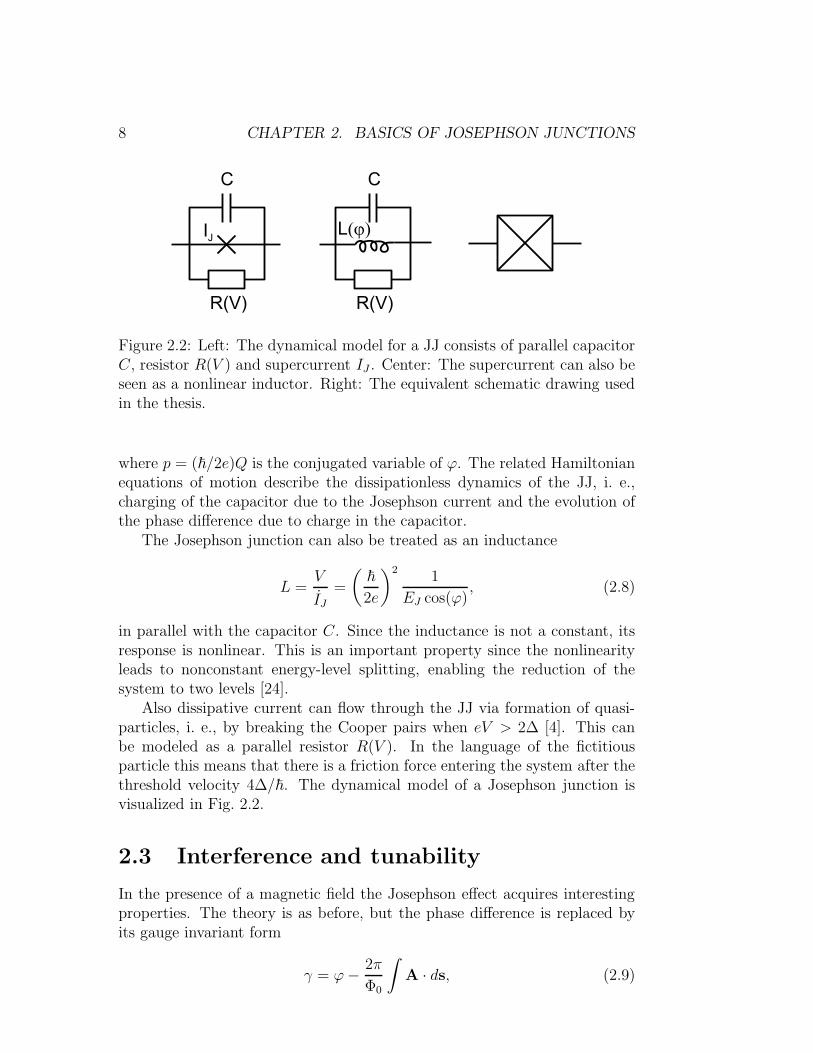
Figure 2.3: Left: The SQUID consists of two parallel JJs. The presence of amagnetic flux can lead to a demand of circulating supercurrent that totallyinhibits the current across the device. Right: A long Josephson junctionpenetrated by a magnetic flux. The current across different parts of the JJcan cancel each other leading to a smaller effective critical current.
where Φ0 = h/2e is the flux quantum, A the vector potential and the inte-gration path is across the insulator. For two parallel JJs the change in thephase ϕ around the superconducting loop must be 2nπ, where n is an arbi-trary integer. Using this one obtains a relation between the phase differencesγi, Fig 2.3, and the magnetic flux Φ through the loop [4],
γ1 − γ2 =2πΦ
Φ0+ n2π. (2.10)
The total current across this superconducting quantum interference device(SQUID) can then be calculated to be
ISQUID = IC1 sin(γ1) + IC2 sin(γ2) = (IC1 + IC2) sin(ϕ) cos
(
πΦ
Φ0
+ nπ
)
+|IC1 − IC2| cos(ϕ) sin
(
πΦ
Φ0+ nπ
)
, (2.11)
where ϕ = (γ1 + γ2)/2 is the effective phase difference of the SQUID. Thecurrents across the individual JJs can cancel each other leading to that theSQUID works effectively as a tunable single JJ. Especially if IC1 = IC2
the currents (and the Josephson coupling energies) can cancel each othercompletely. The essential feature is the periodicity of the Josephson currentas a function of the phase difference. Very sensitive magnetic field detectorsare based on this effect [4]. The tunability of SQUIDs plays a central rolealso in the studies presented in this thesis.
Similarly, in a very long JJ whose electrodes are aligned with the appliedmagnetic field, Fig. 2.3, the currents across different positions can cancel
10 CHAPTER 2. BASICS OF JOSEPHSON JUNCTIONS
each other. In the case of rectangular junctions the effective critical currentcan be put to the form
IC(Φ) = IC(0)| sin (πΦ/Φ0) |
πΦ/Φ0, (2.12)
which is called the Fraunhofer diffraction pattern in analogy to similar lightdiffraction across a rectangular slit.
2.4 Secondary macroscopic quantum effects
In the preceding treatment we assumed that ϕ is a classical variable. Thephase difference can also have quantum fluctuations in proper conditions. Asin all systems, this occurs if environmental noise can be made small whencompared to the energy scale of the quantum effects. The thermal noise islowered by going to very low temperatures and the damping is lowered byisolating the Josephson junction from its nearby environment. The energyscale of the quantum effects can be increased, for example, by lowering thecapacitance C, i.e., going to smaller JJs. If the Josephson coupling energy iskept large, the values C ∼ 1 pF are enough. If EJ is wanted to be smallerthan the (single) charging energy EC = e2/2C, capacitances in the fF rangeneed to be obtained. The conditions are met for mesoscopic JJs that arecooled approximately to 0.1 K.
A straight forward way to find the Hamiltonian operator and the eigen-states of a JJ that is not connected to its environment (isolated JJ) wouldbe the standard quantization of the Hamiltonian function (2.7). This leadsto the commutation relation
[ϕ,Q] = 2ei, (2.13)
where ϕ and Q are now operators. However, the phase difference is a pe-riodic variable and handling it requires more caution [28]. For an isolatedJJ only 2π-periodic wave functions ψ(ϕ) are physical, corresponding to 2equantization of the charge [27]. The problem can be formulated in this spaceby writing the Josephson coupling energy as
EJ = −EJ
2
(
eiϕ + e−iϕ)
, (2.14)
which is quantized in the charge basis |Q〉 as
EJ = −EJ
2
∑
Q
(|Q+ 2e〉〈Q| + |Q− 2e〉〈Q|) . (2.15)
We obtain that the quantized Josephson effect corresponds to coherent single-Cooper-pair tunneling of across the insulator. This operator form is valid as
2.4. SECONDARY MACROSCOPIC QUANTUM EFFECTS 11
-10
0
10
20
0 0.2 0.4 0.6 0.8 1
E/E
C
EJ/EC = 10
q/2e
0
4
8
12
16
0 0.2 0.4 0.6 0.8 1
EJ/EC = 1
q/2e
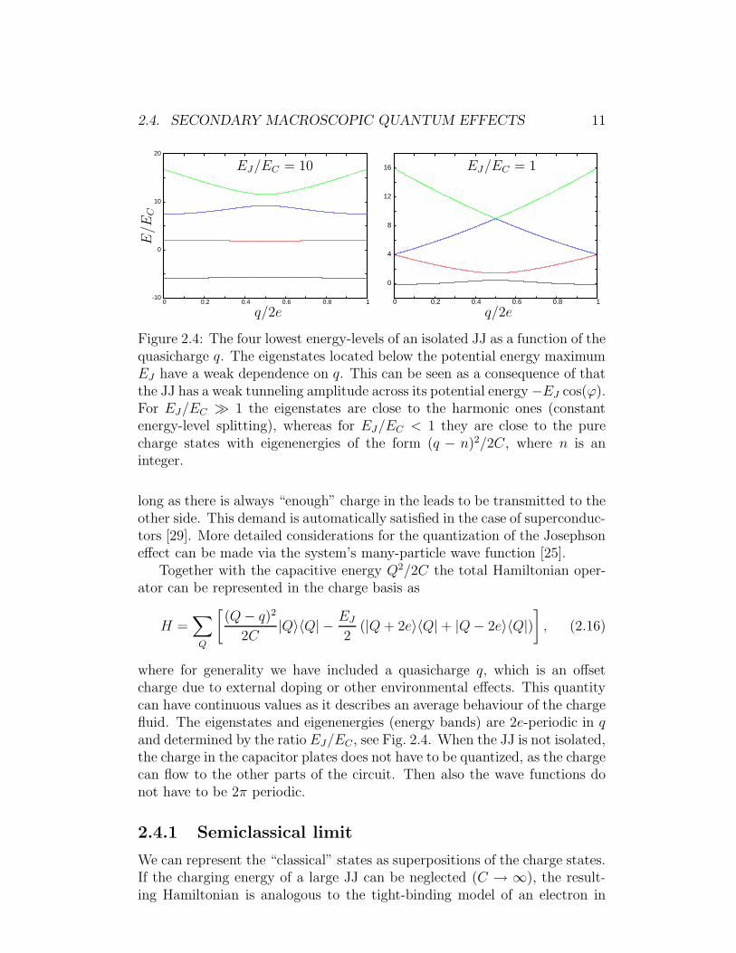
Figure 2.4: The four lowest energy-levels of an isolated JJ as a function of thequasicharge q. The eigenstates located below the potential energy maximumEJ have a weak dependence on q. This can be seen as a consequence of thatthe JJ has a weak tunneling amplitude across its potential energy −EJ cos(ϕ).For EJ/EC ≫ 1 the eigenstates are close to the harmonic ones (constantenergy-level splitting), whereas for EJ/EC < 1 they are close to the purecharge states with eigenenergies of the form (q − n)2/2C, where n is aninteger.
long as there is always “enough” charge in the leads to be transmitted to theother side. This demand is automatically satisfied in the case of superconduc-tors [29]. More detailed considerations for the quantization of the Josephsoneffect can be made via the system’s many-particle wave function [25].
Together with the capacitive energy Q2/2C the total Hamiltonian oper-ator can be represented in the charge basis as
H =∑
Q
[
(Q− q)2
2C|Q〉〈Q| − EJ
2(|Q+ 2e〉〈Q| + |Q− 2e〉〈Q|)
]
, (2.16)
where for generality we have included a quasicharge q, which is an offsetcharge due to external doping or other environmental effects. This quantitycan have continuous values as it describes an average behaviour of the chargefluid. The eigenstates and eigenenergies (energy bands) are 2e-periodic in qand determined by the ratio EJ/EC , see Fig. 2.4. When the JJ is not isolated,the charge in the capacitor plates does not have to be quantized, as the chargecan flow to the other parts of the circuit. Then also the wave functions donot have to be 2π periodic.
2.4.1 Semiclassical limit
We can represent the “classical” states as superpositions of the charge states.If the charging energy of a large JJ can be neglected (C → ∞), the result-ing Hamiltonian is analogous to the tight-binding model of an electron in
12 CHAPTER 2. BASICS OF JOSEPHSON JUNCTIONS
a periodic ion-lattice. The nearby electron sites can be visualized as seriespotential minimums between series barriers. The sites correspond to differentnumber of transmitted pairs. The eigenstates of an isolated JJ are then ofthe form
|ϕ〉 = N∑
Q
|Q〉eiϕQ/2e, (2.17)
where N is a normalization factor. The related eigenenergies are
E(ϕ) = −EJ cos(ϕ). (2.18)
The different values of ϕ correspond to different velocities of the fictitiouselectron (wave packet) in the ion lattice, or equivalently different values forthe current across the JJ. The classical current is therefore
I =2e
~
∂E(ϕ)
∂ϕ= IC sinϕ = IJ . (2.19)
Using the analogy with electron in the ion lattice, it seems natural that largeJJs with small charging energies are driven to these states when interactingwith classical surroundings. For large C (not infinitely large) the differentsites have now different energies and the eigenstates are more Gaussian-type distributions (eigenstates of a harmonic oscillator) but with quite denseenergy-level spacing, which still allows an easy construction of states withalmost localized ϕ. The environment “senses” average values of the cur-rent across the JJ rather than small fluctuations of the local voltage Q/C.The classical analysis fails for small C as quantum-mechanical effects due tonotable energy-level splittings start to dominate.
Chapter 3
Dissipative quantum mechanics
The quantum mechanics and the classical mechanics with dissipation seemto contradict each other. As the expectation value of energy in an isolatedquantum system is a constant, the classical undriven damped oscillator willloose its energy in dissipation. For example, there seems to be no Lagrangianor Hamiltonian description for a velocity dependent friction of a damped os-cillator. However, all the systems must follow the same laws of physics, andthe dissipation in a damped oscillator originates in the coupling of the oscilla-tor’s degrees of freedom to microscopic modes in the surroundings [30]. Theoscillator’s energy is transferred to these modes and in the case of a “large”environment it does not return. The effect can be imitated in the Hamilto-nian description by introducing an environmental Hamiltonian Henv and aninteraction term Hint between the environment and the system H0 [31]. Itis then required that in the classical limit the equations of motion (for themain degree of freedom) reduce to the classical ones with the same frictionalterms. As we do not have the calculational power to describe the surround-ing universe exactly, always something has to be approximated. Typicalapproximations are a thermal equilibrium of the whole system, or some partof it, linear coupling between the environment and the subsystem, quadraticenvironmental Hamiltonian and so on. With the help of simplifying relationsthe quantities related to the subsystem can be calculated via, e.g., seriesexpansion of the systems time-evolution operator. Such a treatment is veryuseful in problems dealing with macroscopic quantum coherence.
3.1 Reduced equation of motion
If there would be no interaction between the system and the environment, theHamiltonian of the total system would beH0+Henv. The total density matrixhas the product form ρtotal = ρ ⊗ ρenv at all times, where ρ is the system’sdensity matrix, if this is true at the initial time. Turning the interaction part
13
14 CHAPTER 3. DISSIPATIVE QUANTUM MECHANICS
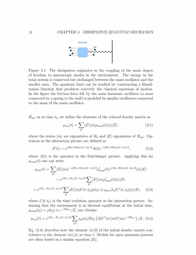
Figure 3.1: The dissipation originates in the coupling of the main degreeof freedom to microscopic modes in the environment. The energy in thetotal system is conserved but exchanged between the main oscillator and thesmaller ones. The quantum limit can be studied by constructing a Hamil-tonian function that produces correctly the classical equations of motion.In the figure the friction force felt by the main harmonic oscillator (a massconnected by a spring to the wall) is modeled by smaller oscillators connectedto the mass of the main oscillator.
Hint on at time t0, we define the elements of the reduced density matrix as
ρmn(t) =∑
E
〈E|〈m|ρtotal(t)|n〉|E〉, (3.1)
where the states |m〉 are eigenstates of H0 and |E〉 eigenstates of Henv. Op-erators in the interaction picture are defined as
AI(t) = ei(H0+Henv)(t−t0)/~A(t)e−i(H0+Henv)(t−t0)/~, (3.2)
where A(t) is the operator in the Schrodinger picture. Applying this forρtotal(t) one can write
ρmn(t) =∑
E
〈E|〈m|e−i(H0+Henv)(t−t0)/~ρItotal(t)e
i(H0+Henv)(t−t0)/~|n〉|E〉
= ei(En−Em)(t−t0)/~∑
E
〈E|〈m|ρItotal(t)|n〉|E〉
= ei(En−Em)(t−t0)/~∑
E
〈E|〈m|U(t, t0)ρ(t0) ⊗ ρenv(t0)U†(t, t0)|n〉|E〉, (3.3)
where U(t, t0) is the time evolution operator in the interaction picture. As-suming that the environment is in thermal equilibrium at the initial time,ρtotal(t0) = ρ(t0) ⊗ e−βHenv/Z, one obtains
ρmn(t) = ei(En−Em)(t−t0)/~∑
a,b
ρab(t0)TrE
(
〈b|U †|n〉〈m|U |a〉e−βHenv
)
/Z. (3.4)
Eq. (3.4) describes how the element |a〉〈b| of the initial density matrix con-tributes to the element |m〉〈n| at time t. Models for open quantum-systemsare often based on a similar equation [31].
3.1. REDUCED EQUATION OF MOTION 15
3.1.1 Expanding the time-evolution operator
We proceed from Eq. (3.4) by determining U(t, t0). The time evolution inthe interaction picture follows the Schrodinger equation
i~∂
∂t|ψ(t)〉I = HI
int(t)|ψ(t)〉I . (3.5)
If the operator HIint(t) commutes with itself at different times, the formal
solution of Eq. (3.5) is
|ψ(t)〉I = U(t, t0)|ψ(t0)〉I = e−i
R t
t0HI
int(t′)dt′/~|ψ(t0)〉I . (3.6)
However, this assumption cannot be made in situations considered and wemust use the most general solution
|ψ(t)〉I = U(t, t0)|ψ(t0)〉I = T−e−i
R t
t0HI
int(t)dt/~|ψ(t0)〉I
=
[
1 +∞∑
n=1
(−i~
)n ∫ t
t0
dt1
∫ t1
t0
dt2 . . .
∫ tn−1
t0
dtnHIint(t1) . . .H
Iint(tn)
]
|ψ(t0)〉I .
(3.7)
The special order of integration (defining the time-ordering operator T−) as-sures that t > t1 > t2 · · · > tn > t0. The time ordering of U †(t, t0) is reversed.Insertion of Eq. (3.7) into Eq. (3.4) results in infinite summation of variousterms describing all the physics that can occur at the intermediate times.Such summations can usually be rewritten more efficiently as diagrams, eachof them representing a contribution in the sum [32, 33].
3.1.2 Route to the diagrammatic formulation
To illustrate where the diagrammatic formulation originates, let us considerthe case the interaction part is of the (bi)linear form Hint = Qq, where Qis related to the system and q to the environment. In expansion (3.7) theconstant 1 evidently describes a process where no interaction with the envi-ronment (transitions) takes place. The first-order term −i
∫ t
t0dt1Q(t1)q(t1)/~
corresponds to a process where a single transition occurs and a summa-tion (integration) over all the possible transition times is performed. Thesecond-order term −
∫ t
t0dt1∫ t1
t0dt2Q(t1)q(t1)Q(t2)q(t2)/~
2 is a process wheretwo transitions take place, the first at time t2 and the second at time t1, andso on. The operator U(t, t0)
† includes the same terms but in a time reversedfashion, as the order of the Hamiltonians HI
int(ti) is reversed.The expansion of the two time-evolution operators in Eq. (3.4) shows that
the final element is a sum of all the possible transitions at the intermediatetimes with certain amplitudes. The summation represents the fact that the
16 CHAPTER 3. DISSIPATIVE QUANTUM MECHANICS
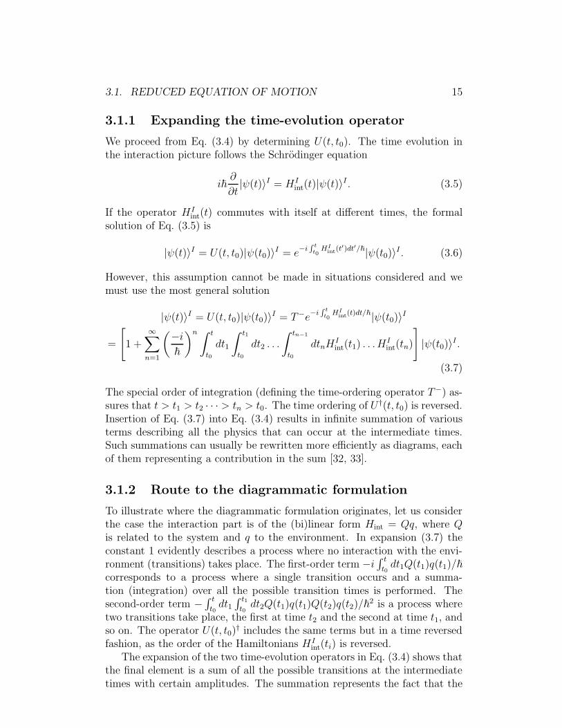
Figure 3.2: A Keldysh-type diagrammatic visualisation [34, 35, 36, 37] of afourth-order term in Eq. (3.4). The upper branch corresponds to the forward-time propagation and the lower to the backward-time propagation. Twoterms originate in matrix elements of U and two terms in U †. In this casethe environment groups the interaction points to pairs by environmental lines.This is one of the three possibilities how the four points can be grouped.
quantum-mechanical evolution can be understood as a sum of all the possible“paths” [32]. However, in the studied case we do not consider the environ-mental states separately, since in Eq. (3.4) we do a trace over the environmen-tal degrees of freedom. This reduces the environmental operators to correla-tion functions such that 〈〈q(t)q(t′)q(t′′)〉〉, which are usually known quantitiesas they can be calculated from the initial thermal distribution. This is a gen-eral result for the initial product-state density-matrix. If the environmentalHamiltonian is also quadratic, the Wick’s theorem [38] assures that the tracecan be represented using only pair correlations α(t − t′) = 〈〈q(t)q(t′)〉〉 andthat odd correlations vanish. It follows that Eq. (3.4) is a sum of all the pos-sible transitions with arbitrary pair correlations, Fig. 3.2. Also cases wherethe Wick’s theorem cannot be applied, and odd moments do not vanish, haveattracted more attention recently [39].
3.1.3 Master equation
Usually one represents Eq. (3.4) as a master equation by differentiating itwith respect to time. The differentiation, when focusing on the operatorU (†), annihilates (the constant 1 and) the integration over the variable t1 andleads to the substitution t1 = t. It results that the processes always end to atransition at time t. One obtains formally
ρmn(t) = i(En − Em)ρmn(t)/~ +∑
a,b
Γa→mb→n ρab(t0), (3.8)
3.1. REDUCED EQUATION OF MOTION 17
where the first term in the r.h.s. describes the quantum-mechanical evolu-tion in the case Hint = 0. The interaction with the environment inducestransitions described by the transition-rate tensor Γ including all diagramsstarting at time t0 and ending to a transition at time t.
Except that every diagram ends to a transition at time t, consider nowa diagram which is also irreducible between times t′ > t0 and t, meaningthat any vertical line at time t, t′ < t < t cuts at least one environmentalline. For example, the fourth-order diagram in Fig. 3.2 is irreducible betweenthe times τ2 and t1. It cannot be cut to half in this region. Because thereis generally a transition at time t, every diagram starting from t0 ends toan irreducible part between certain times t′′ and t. On the other hand, afixed irreducible diagram between the times t′ and t can have an arbitrary“starting” part between the times t0 and t′. The formal summation of allthe possible diagrams from t0 to t′ gives the element ρa′b′(t
′). Summing up(integrating) all the possible times t′ and intermediate states one obtains theequivalent form of Eq. (3.8) (by marking a′ = a and b′ = b)
ρmn(t) = i(En − Em)ρmn(t)/~ +∑
a,b
∫ t
t0
dt′Σa→mb→n (t− t′)ρab(t
′), (3.9)
where the function (self-energy matrix) Σa→mb→n (t−t′) is a sum of all irreducible
diagrams starting from t′ and ending to t. This is the master equation in itsmost general form.
Born approximation
Often Eq. (3.9) needs to be simplified for practical calculations. If the in-teraction with the environment is weak, one can cut the diagrammatic sum-mation to include at most certain order diagrams in HI
int. The lowest-orderapproximation is called the Born approximation, where only the second-orderdiagrams are considered. The naming “weak” can lead to misconception ofminor effects, as the interaction can still drastically interfere the quantum co-herence in the system. By cutting Eq. (3.9) to include only few diagrams, theassumption of the product-state density-matrix at the initial time t0 (Section3.1) is effectively made for all times. This is actually a good approximationin situations where the macroscopic environment is only slightly perturbedby the interaction with the system.
Markov approximation
The master equation (3.9) is an integro-differential equation as both thedifferentiation and the integration with respect to time exists simultaneously.The Markov approximation aids in solving the equation by dropping thehistory out of the equation. This can be done by assuming that ρ(t′) on the
18 CHAPTER 3. DISSIPATIVE QUANTUM MECHANICS
r. h. s. of Eq. (3.9) can be substituted by the interaction-picture (backward)time-evolution of ρ(t)
ρ(t′) ≈ exp[iH0(t− t′)/~]ρ(t) exp[−iH0(t− t′)/~]. (3.10)
The assumption is valid if environmental memory loss is fast when comparedto the timescale of transitions. Together with the Born approximation andthe limit t0 → −∞ the master equation gets the Born-Markov (BM) form
ρmn(t) = i(En −Em)ρmn(t)/~ +∑
a,b
Γa→mb→n ρab(t), (3.11)
where Γ is the generalized transition-rate tensor in the golden-rule approxi-mation [31].
Lindblad approximation
The truncation of the diagrammatic summation, and perhaps dropping outthe history, are great simplifications for the master equation and in mostcases vital for practical calculations. But they can also lead to problems, asthe truncated equation of motion is rather phenomenological and there is noguarantee that the solution describes any physical system anymore. The BMequation preserves the trace of the density matrix but can, in the worst case,lead to large negative values for (some of) the populations. Such effects areto be expected, for example, in the region where the Born and/or Markovapproximations are starting to fail. The most safe way to do master-equationsimulations is to resort to the general form of the master equation that pre-serves the positivity of the density matrix, i.e., to the Lindblad form [40]
ρ = −i[H0, ρ]/~ +∑
i
(LiρL†i −
1
2L†iLiρ−
1
2ρL†iLi), (3.12)
where the operators Li describe transitions between the eigenstates
Li =∑
mn
γim←n|m〉〈n|, (3.13)
where γim←n are constant numbers. Generally, the master equation in the
Born-Markov approximation is not of Lindblad type. To dress it into thisform one can either neglect some of the nondiagonal contributions or redefinetheir generalized transition rates. The choice is not unanimous. This “safemode” of the master equation guarantees positivity of the density matrix,but is one further approximation to the original equation. Therefore a carefulanalysis is recommended before “choosing” the Lindblad form of the masterequation, as a wrong Lindblad-type can loose important effects. Some masterequations cannot be recast to the Lindblad form without loosing the essentialphysics they describe. Therefore also investigations of other reliable masterequations are actively done [41, 42].
3.2. ENVIRONMENTS 19
3.2 Environments
We will now study the Hamiltonian formalisms of the dissipative environ-ments considered in the thesis. The first environment is the electromagneticenvironment (EE) which is basically formed by the leads and external cir-cuitry attached to the JJ. The second environment consists of quasiparticledegrees of freedom, i. e., unpaired electrons in the superconductors. Thethird environment describes spurious charge fluctuators (CF) in the nearbymaterials of the device. The first environment is bosonic whereas the sec-ond consists of fermions. The exact nature of the charge fluctuators is notspecified, as this environment is the least known.
3.2.1 Electromagnetic environment
The electromagnetic environment is a linear environment between the biasand the system and can be characterized by an impedance Z(ω). It canbe modeled as a set of harmonic oscillators coupled bilinearly to the sys-tem [31]. One has generally two choices for the modeling: whether to couplethe environment to a phase-like variable or to a charge like. The methodsare equivalent. The aim is to derive the correct Langevin equation for thesystem.
Let us consider the case when the environment is coupled to the phasevariable of a Josephson junction. We write the Hamiltonian of the totalsystem as
H =Q2
2C−EJ cos(ϕ) +
N∑
α=1
[
q2α
2Cα+
(
~
2e
)2(ϕ− ϕα)2
2Lα
]
, (3.14)
where [ϕ,Q] = 2ei, [ϕα, qα] = 2ei and the cross commutators vanish. Weidentify the interaction
Hint = −(
~
2e
)2
ϕ
(
N∑
α=1
1
Lαϕα
)
, (3.15)
a term often referred as the “renormalization” of H0 [30]
Hrn =
(
~
2e
)2
ϕ2
(
N∑
α=1
1
2Lα
)
, (3.16)
and the environmental Hamiltonian
Henv =
N∑
α=1
[
q2α
2Cα+
(
~
2e
)2ϕ2
α
2Lα
]
. (3.17)

20 CHAPTER 3. DISSIPATIVE QUANTUM MECHANICS
Figure 3.3: The Josephson junction in parallel with an impedance Z(ω) (left)and its equivalent circuit (right) where the impedance is constructed froman infinite number of parallel series-LC-oscillators.
Hamiltonian (3.14) describes a dissipationless Josephson junction in parallelwith series-LC-oscillators. The aim is to show that the oscillators produceany desired frequency dependent impedance Z(ω), see Fig. 3.3.
The Heisenberg equations of motion for the total system read
ϕ =1
C
2e
~IC sin(ϕ) − 1
C
N∑
α=1
(
ϕ− ϕα
Lα
)
(3.18)
ϕα = −ω2α(ϕα − ϕ). (3.19)
Regarding ϕ(t) as a given operator in time, the formal solution for ϕα(t) canbe written as
ϕα(t) = ϕα(t0) cos(ωαt) +2e
~
1
ωαCαqα(t0) sin(ωαt)+
ωα
∫ t
t0
dt′ sin[ωα(t− t′)]ϕ(t′). (3.20)
To obtain an expression where the “velocity” is present, we integrate the lastterm by parts and obtain
ϕα(t) = ϕα(t0) cos(ωαt) +2e
~
1
ωαCαqα(t0) sin(ωαt)
+ϕ(t) − ϕ(t0) cos(ωαt) −∫ t
t0
dt′ cos[ωα(t− t′)]ϕ(t′). (3.21)
3.2. ENVIRONMENTS 21
Then substituting this into the equation of motion for ϕ we obtain
Cϕ(t) =2e
~IC sin[ϕ(t)] −
∫ t
t0
dt′N∑
α=1
cos[ωα(t− t′)]
Lαϕ(t′)
−N∑
α=1
cos(ωαt)
Lαϕ(t0)
+N∑
α=1
ϕα(t0)cos(ωαt)
Lα
+2e
~
N∑
α=1
ωαqα(t0) sin(ωαt). (3.22)
The first term on the r.h.s. of Eq. (3.22) describes the Josephson currentacross the JJ whereas the second term is a memory-friction term, relatedto the Fourier-transformed admittance Y (ω) in this situation. The last linerepresents fluctuations, i. e., the random force generated by the environment.The values (or in quantum case the operators) ϕα(0) and qα(0) are takenfrom a proper statistical ensemble. The third term is spurious and dependson the initial value of ϕ. It has been shown that it is an artefact of theinitial decoupling of the environment and the subsystem. However, it can beincluded in the random force by a careful definition of the statistical ensemble(and therefore we neglect it) [31]. One obtains the quantum mechanicalversion of the current balance (Langevin) equation for the Josephson junctionin parallel with the impedance Z(ω)
ϕ(t) +1
C
∫ t
t0
dt′Y (t− t′)ϕ(t′) − 1
C
2e
~IC sin(ϕ) =
2e
~
1
CIn (3.23)
Y (t) =N∑
α=1
cos(ωαt)
Lα
Θ(t) (3.24)
In =~
2e
N∑
α=1
ϕα(t0)cos(ωαt)
Lα+
N∑
α=1
ωαqα(t0) sin(ωαt), (3.25)
where Θ(t) is the step function. Clearly any kind of admittance can bemodeled by the proper choice of parameters Lα. By directly calculating theFourier transform (lims→0
∫
dteiωt−s|t|) of Y (t) one obtains
Z(−ω)−1 = Y (−ω) = lims→0
N∑
α=1
1
2Lα
[
i
ω + ωα + is+
i
ω − ωα + is
]
, (3.26)
which defines the variables Lα and Cα.
3.2.2 Quasiparticles
Quasiparticles in the superconductor are electrons that are not bound toCooper pairs. They behave similarly as electrons in the normal metal and
22 CHAPTER 3. DISSIPATIVE QUANTUM MECHANICS
also feel the presence of the condensate. The quasiparticles in the lead r(quasiparticle reservoir) can be described by the Hamiltonian [4]
Hrqp =
∑
k,i
Ekrγ†kirγkir, (3.27)
where the operators γ(†)kir are excitation annihilation (creation) operators with
momentum k and spin degree of freedom i. They satisfy the fermionic anti-commutation relations. The eigenenergies of the excitations are
Ekr = (ǫ2k + ∆2r)
1/2, (3.28)
where ǫk is the energy of the corresponding normal metal quasiparticle statemeasured from the Fermi level. It is assumed to depend only on the lengthof k. The minimum energy for creating an excitation is ∆r. Because thereis one to one correspondence with the normal metal states, the density ofstates in the superconducting case can be shown to be
N rsc(E) =
Ekr√
E2kr − ∆2
r
N r0 , (3.29)
where N r0 is the normal metal density of states at the Fermi surface. In
thermal equilibrium the excitations are present according to the probability(Fermi) distribution
f(Ekr) =1
1 + eβEkr. (3.30)
Two nearby leads with a tunnel junction in between interact by exchang-ing electrons and by an electric field described earlier via capacitance C. Inthe case of low transparency junctions the electron tunneling can be mod-eled using the tunneling Hamiltonian formalism [23]. It describes an electronpropagation across the insulating barrier as the interaction
HT =∑
k,l,i
[Tkla†ki1ali2 + h.c.], (3.31)
where a(†)kir is the electron annihilation (creation) operator of the state k with
the spin degree of freedom i and Tkl is the tunneling amplitude. If themotion of the particles is ballistic, one obtains for the transmission across arectangular barrier with height U and width L [23]
|Tkl|2 =1
4π2
δk||,l||
ρ2exp
(
−2L
~
√
2mU − k||
)
, (3.32)
where ρ is the one dimensional density of states in metals perpendicular to thebarrier. The transverse momentum (k||) is conserved. According to the BCS
3.2. ENVIRONMENTS 23
theory [22, 4] the quasiparticle operators have the relation ak↑ = u∗kγk0+vkγ†k1
and a−k↓ = −vkγ†k0 + u∗kγk1, where uk and vk are superconducting coherence
factors satisfying
|uk|2 =1
2
(
1 +ǫkEkr
)
(3.33)
|vk|2 =1
2
(
1 − ǫkEkr
)
= 1 − |uk|2. (3.34)
The effect ofHT can be analyzed, for example, by using a master-equationapproach similar as in Section 3.1. In the lowest-order calculation one obtainsterms of the form
a†k↑ak↑ = |uk|2γ†k0γk0 + |vk|2γk1γ
†k1, (3.35)
describing quasiparticle tunneling across the Josephson junction. Also termslike
ak↑a−k↓ = −u∗kvkγk0γ†k0 + vku
∗kγ†k1γk1, (3.36)
exist describing the Josephson effect. The terms (3.36) are already taken intoaccount as the potential energy −EJ cos(ϕ) and therefore their contributionis neglected. The expression (3.35) includes two terms with superconductingcoherence factors uk and vk. However, for every k there is a momentum k′ forwhich Ek = Ek′ but k 6= k′ and |u(k′)|2 = |v(k)|2. Since |u(k)|2 + |v(k)|2 = 1the factors u and v vanish from the final expressions (in the lowest-ordertreatment). Further, the first term on the r.h.s. of Eq. (3.35) contributesif the state is occupied, i.e., by the factor f(Ek) and the second one if thestate is empty, i.e., by the factor 1 − f(Ek). Since 1 − f(Ek) = f(−Ek)the contribution of the second term can be included to the first one in theequivalent semiconductor picture [4], where the energies (3.28) of the stateswhose momentum lies below the Fermi surface are reversed. In such a modelno coherence factors exists and by the special energy spectrum it is assuredthat the same elements are not summed twice.
Linking the factors Tkl to the normal state behaviour [23, 4] one obtainsfor the net quasiparticle current between two voltage-biased superconductorsin the semiconductor picture
Iss(V ) =1
eRT
∫ ∞
−∞
|E|√
E2 − ∆21
|E + eV |√
(E + eV )2 − ∆22
[f(E) − f(E + eV )]dE,
(3.37)
where the integration excludes the values such that |E| < ∆1 and |E +eV | < ∆2. Generally, for a given temperature this have to be calculatednumerically, but behaves approximately as Iss(V ) ∼ Θ(|eV |−∆1−∆2)V/RT .
24 CHAPTER 3. DISSIPATIVE QUANTUM MECHANICS
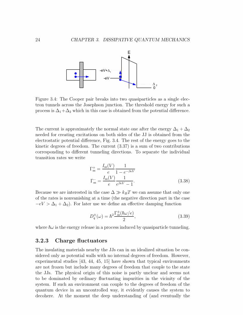
Figure 3.4: The Cooper pair breaks into two quasiparticles as a single elec-tron tunnels across the Josephson junction. The threshold energy for such aprocess is ∆1+∆2 which in this case is obtained from the potential difference.
The current is approximately the normal state one after the energy ∆1 + ∆2
needed for creating excitations on both sides of the JJ is obtained from theelectrostatic potential difference, Fig. 3.4. The rest of the energy goes to thekinetic degrees of freedom. The current (3.37) is a sum of two contributionscorresponding to different tunneling directions. To separate the individualtransition rates we write
Γ+ss =
Iss(V )
e
1
1 − e−βeV
Γ−ss =Iss(V )
e
1
eβeV − 1. (3.38)
Because we are interested in the case ∆ ≫ kBT we can assume that only oneof the rates is nonvanishing at a time (the negative direction part in the case−eV > ∆1 + ∆2). For later use we define an effective damping function
D±q (ω) = ~2Γ±ss(~ω/e)
2, (3.39)
where ~ω is the energy release in a process induced by quasiparticle tunneling.
3.2.3 Charge fluctuators
The insulating materials nearby the JJs can in an idealized situation be con-sidered only as potential walls with no internal degrees of freedom. However,experimental studies [43, 44, 45, 15] have shown that typical environmentsare not frozen but include many degrees of freedom that couple to the statethe JJs. The physical origin of this noise is partly unclear and seems notto be dominated by ordinary fluctuating impurities in the vicinity of thesystem. If such an environment can couple to the degrees of freedom of thequantum device in an uncontrolled way, it evidently causes the system todecohere. At the moment the deep understanding of (and eventually the
3.2. ENVIRONMENTS 25
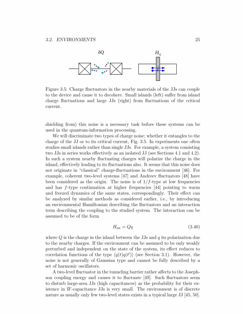
Figure 3.5: Charge fluctuators in the nearby materials of the JJs can coupleto the device and cause it to decohere. Small islands (left) suffer from islandcharge fluctuations and large JJs (right) from fluctuations of the criticalcurrent.
shielding from) this noise is a necessary task before these systems can beused in the quantum-information processing.
We will discriminate two types of charge noise; whether it entangles to thecharge of the JJ or to its critical current, Fig. 3.5. In experiments one oftenstudies small islands rather than single JJs. For example, a system consistingtwo JJs in series works effectively as an isolated JJ (see Sections 4.1 and 4.2).In such a system nearby fluctuating charges will polarize the charge in theisland, effectively leading to its fluctuations also. It seems that this noise doesnot originate in “classical” charge-fluctuations in the environment [46]. Forexample, coherent two-level systems [47] and Andreev fluctuators [48] havebeen considered as the origin. The noise is of 1/f -type at low frequenciesand has f -type continuation at higher frequencies [44] pointing to warmand freezed dynamics of the same states, correspondingly. Their effect canbe analyzed by similar methods as considered earlier, i.e., by introducingan environmental Hamiltonian describing the fluctuators and an interactionterm describing the coupling to the studied system. The interaction can beassumed to be of the form
Hint = Qq (3.40)
where Q is the charge in the island between the JJs and q its polarization dueto the nearby charges. If the environment can be assumed to be only weaklyperturbed and independent on the state of the system, its effect reduces tocorrelation functions of the type 〈q(t)q(t′)〉 (see Section 3.1). However, thenoise is not generally of Gaussian type and cannot be fully described by aset of harmonic oscillators.
A two-level fluctuator in the tunneling barrier rather affects to the Joseph-son coupling energy and causes it to fluctuate [49]. Such fluctuators seemto disturb large-area JJs (high capacitances) as the probability for their ex-istence in fF-capacitance JJs is very small. The environment is of discretenature as usually only few two-level states exists in a typical large JJ [45, 50].
26 CHAPTER 3. DISSIPATIVE QUANTUM MECHANICS
3.3 Fluctuations in a linear system
3.3.1 Fluctuation-dissipation theorem
A dissipative system in thermal equilibrium performs random fluctuationsthat are a counterpart of the damping. They can be viewed as random forceskicking the system out of its ground state into which the damping is tryingto drive it. The system’s relaxation to the equilibrium after external forcingis described by the dynamical susceptibility which can be related to theequilibrium fluctuations via the famous fluctuation-dissipation theorem [51](FDT). The FDT has a central role in many studies that consider the effectof a noisy environment to the system under study.
Consider voltage fluctuations in a circuit that consists of a capacitor Cand an impedance Z(ω). From Section 3.1 we know that the Hamiltonianof the total system is quadratic and the equations of motion linear. Fora linear system the FDT holds exactly and due to Ehrenfest theorem it issufficient to consider only classical equations of motion for determining thedynamical susceptibility [31]. Let us choose the arbitrary force f(t) to be adelta function at an infinitesimal time after the initial time, before which thesystem is in the equilibrium Qe = 0. Then for arbitrary times we have thevoltage-balance equation
Q(t)
C+
∫ t
0
Z(t− t′)I(t′)dt′ = Q0δ+(t), (3.41)
where the Fourier transform of the kernel Z(t) is the impedance Z(−ω) andI = Q. By Laplace transforming Eq. (3.41) one obtains
Q(s)
C+ Z(−is)(sQ(s) −Qe) = Q0, (3.42)
which can be recast to the form (using Qe = 0)
Q(s) =Q0
1C
+ sZ(−is) . (3.43)
The dynamical susceptibility S(t) is defined as the linear response Q(t) =Q0S(t) and one obtains
∫ ∞
0
S(t)eiωtdt =1
1C− iωZ(−ω)
≡ ZQ(ω). (3.44)
The quantum FDT relates the equilibrium fluctuations of V to S(t) as
∫ ∞
−∞
eiωt〈V (t)V (0)〉dt =2~
1 − e−~ωβ
Im[ZQ(ω)]
C2, (3.45)
3.3. FLUCTUATIONS IN A LINEAR SYSTEM 27
where we have used that Q = CV . For Z(ω) = R one obtains an importantresult
∫ ∞
−∞
eiωt〈V (t)V (0)〉dt =2~ω
1 − e−~ωβ
R
1 +(
ωωc
)2 , (3.46)
where ωc = 1/RC is the cut-off frequency of the voltage fluctuations.Similarly, we can always define a phase-difference operator related to the
voltage V as
ϕ =2eV
~=
2e
~
Q
C, (3.47)
described by the classical current balance equation
C~
2eϕ(t) +
∫ t
−∞
dt′Y (t− t′)~
2eϕ(t′) = 0, (3.48)
where Y (t) is related to the admittance Y (ω) = 1/Z(ω). This is the Langevinequation of a quantum Brownian motion. Via a similar calculation as we didfor the voltage fluctuations one obtains
∫ ∞
−∞
eiωt〈ϕ(t)ϕ(0)〉dt =2~
1 − e−~ωβIm[Zϕ(ω)] (3.49)
Zϕ(ω) = − 1
Cω2 + iωY (−ω). (3.50)
Again for the ohmic resistor∫ ∞
−∞
eiωt〈ϕ(t)ϕ(0)〉dt =1
ω
2~
1 − e−~ωβ
R
1 +(
ωωc
)2 . (3.51)
The spectrum diverges for ω → 0 and 〈ϕ(t)ϕ(0)〉 diverges for all times. Thisis natural since Brownian motion of a free particle is not restricted to anypart of the space.
The proper correlation function for considering the phase fluctuations is
J(t) = 〈(ϕ(t) − ϕ(0))ϕ(0)〉, (3.52)
where the diverging part of Brownian motion is subtracted off. By consider-ing the element 〈ϕ(t)ϕ(0)〉 one can derive the result
J(t) = 2
∫ ∞
0
dω
ω
Re[Zt(ω)]
RQ
coth
(
1
2β~ω
)
[cos(ωt) − 1] − i sin(ωt)
,
(3.53)
where RQ = h/4e2 is the resistance quantum and Zt(ω) the tunneling impedance,related to the result (3.50) as
Zt(ω) =1
iωC + 1Z(ω)
= iωZϕ(−ω). (3.54)
28 CHAPTER 3. DISSIPATIVE QUANTUM MECHANICS
3.3.2 Incoherent Cooper-pair tunneling
When the capacitor C is a JJ with a small critical current, the Cooper-pair tunneling can be treated as a perturbation to the equilibrium dynamicsconsidered in Section 3.3.1. In contrast to the case of ordinary coherentCooper-pair tunneling, the process is called incoherent or inelastic. This isbecause one effectively assumes that the (coherent) Cooper-pair tunneling issoon interrupted by an incoherent environmental process. If the JJ and theimpedance Z(ω) are in series with a voltage source V , the process dissipatesthe energy ∼ 2eV released in each of the single-Cooper-pair tunneling events.The tunneling perturbs the environment, but if it can be assumed to relax toits equilibrium before the next tunneling occurs, the current can be calculatedusing the golden-rule treatment, called the P (E)-theory [16]. This importanttheory applies for arbitrary Z(ω) and states that the net current across theJJ is
I = 2eΓ+ − 2eΓ− = 2eπ
2~E2
J [P (2eV ) − P (−2eV )], (3.55)
where
P (E) =1
2π~
∫ ∞
−∞
exp
[
4J(t) +i
~Et
]
, (3.56)
is interpreted as the probability for the energy E to be absorbed/emittedby the dissipative environment in the tunneling process. For |V | 6= 0 anet current can flow only if the energy 2eV (released in the Cooper-pairtunneling) can be dissipated by the environment. It results that the energy-level structure of the environment is seen as peaks in the I−V characteristics.For this reason the voltage-biased small JJ is an excellent tool for probingvarious properties of its nearby environment [52, 53, 18, 19].
Chapter 4
Applications
In this Chapter we go through the basics of the devices studied in Papers I-IV. We also discuss the main results of the Papers and extend some subjectsnot covered. The circuits studied are often not single JJs but rather islands,in order to avoid a direct contact between the device and the leads attachedto the system. At high frequencies the leads act as transmission lines caus-ing unwanted decoherence and dissipation. In general, all the noise sources(Section 3.2) should be shielded as well as possible, if the experiment is notstudying them.
4.1 Cooper-pair box
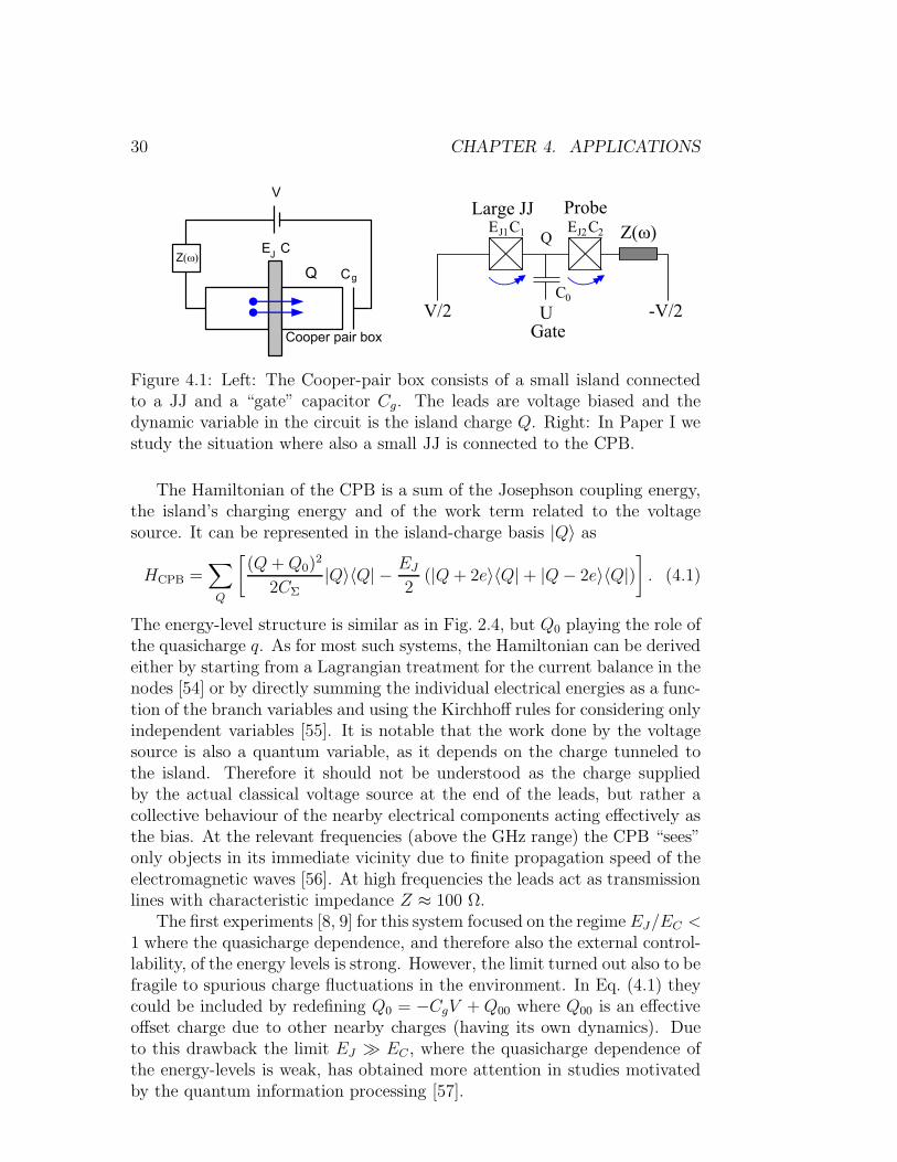
The simplest device that acts analogously to an isolated JJ, but is not ina direct contact with the leads, is probably the Cooper-pair box (CPB),depicted in Fig. 4.1. The mesoscopic island is connected to the outside worldvia a JJ and a gate capacitor. The Cooper pairs can tunnel coherentlythrough the JJ to the island and vice versa. The size of the island is ofmesoscopic scale in order to minimize its capacitance to ground and to makethe lumped circuit model valid. Then the charging energy of the island isdetermined by the capacitance CΣ = C + Cg. The name “box” originatesin that if EJ ∼ EC , usually only a few excess Cooper pairs, as compared tothe background charge, populate the island. The decohering effect of voltagefluctuations due to the impedance Z(ω) is reduced by a factor (Cg/CΣ)2
which can be seen as the JJ’s fraction of the total voltage fluctuations acrossthe CPB to the second power (if the CPB is treated only as two capacitors inseries). The factor can be made very small by going to small gate capacitanceswhile the polarisation charge Q0 = −CgV is kept a constant by increasing V .The first demonstrations on the real-time controllability of the JJ’s quantumstates were performed in this kind of circuit [8, 9]. In these studies also anac-signal or additional voltage pulse was applied to V in order to inducetransitions between the eigenstates of the CPB.
29
30 CHAPTER 4. APPLICATIONS
Figure 4.1: Left: The Cooper-pair box consists of a small island connectedto a JJ and a “gate” capacitor Cg. The leads are voltage biased and thedynamic variable in the circuit is the island charge Q. Right: In Paper I westudy the situation where also a small JJ is connected to the CPB.
The Hamiltonian of the CPB is a sum of the Josephson coupling energy,the island’s charging energy and of the work term related to the voltagesource. It can be represented in the island-charge basis |Q〉 as
HCPB =∑
Q
[
(Q+Q0)2
2CΣ|Q〉〈Q| − EJ
2(|Q+ 2e〉〈Q| + |Q− 2e〉〈Q|)
]
. (4.1)
The energy-level structure is similar as in Fig. 2.4, but Q0 playing the role ofthe quasicharge q. As for most such systems, the Hamiltonian can be derivedeither by starting from a Lagrangian treatment for the current balance in thenodes [54] or by directly summing the individual electrical energies as a func-tion of the branch variables and using the Kirchhoff rules for considering onlyindependent variables [55]. It is notable that the work done by the voltagesource is also a quantum variable, as it depends on the charge tunneled tothe island. Therefore it should not be understood as the charge suppliedby the actual classical voltage source at the end of the leads, but rather acollective behaviour of the nearby electrical components acting effectively asthe bias. At the relevant frequencies (above the GHz range) the CPB “sees”only objects in its immediate vicinity due to finite propagation speed of theelectromagnetic waves [56]. At high frequencies the leads act as transmissionlines with characteristic impedance Z ≈ 100 Ω.
The first experiments [8, 9] for this system focused on the regime EJ/EC <1 where the quasicharge dependence, and therefore also the external control-lability, of the energy levels is strong. However, the limit turned out also to befragile to spurious charge fluctuations in the environment. In Eq. (4.1) theycould be included by redefining Q0 = −CgV +Q00 where Q00 is an effectiveoffset charge due to other nearby charges (having its own dynamics). Dueto this drawback the limit EJ ≫ EC , where the quasicharge dependence ofthe energy-levels is weak, has obtained more attention in studies motivatedby the quantum information processing [57].
4.1. COOPER-PAIR BOX 31
4.1.1 Energy-level probing
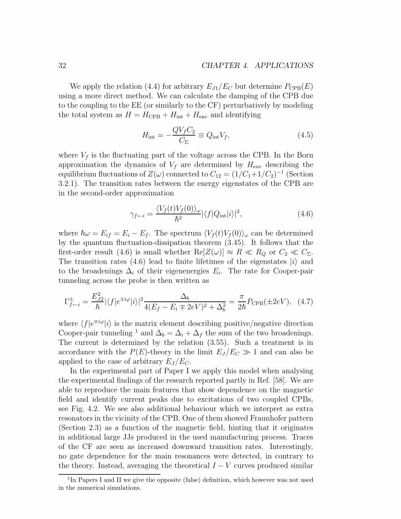
Paper I analyzes a situation where the energy levels of the CPB are probedby incoherent Cooper-pair tunneling through an additional small JJ (probe)attached to the island, Fig. 4.1. A net probe-current is possible if its en-vironment is able to absorb the energy 2eV released in each of the single-Cooper-pair tunneling processes, similarly as in the case of Section 3.3.2.The relevant environment consists of the CPB, of nearby electric-circuitry(EE), and of spurious charge-fluctuators (CF). The study is done in the eyeof the experiment [58] where the larger JJ was realized as a SQUID and thesystem could be studied in situ through a wide range of the ratio EJ1/EC byapplying different magnetic fields to the system.
In the theoretical part of Paper I the current across the probe is calculatedperturbatively. The (unperturbed) Hamiltonian of the CPB is similar as inEq. (4.1) with the changes Q0 ≈ C0U − C2V and CΣ = C0 + C1 + C2.We assume that C0 ≪ C1, C2 so fluctuations of U can be neglected. IfEJ1/EC ≫ 1 the lowest energy-eigenfunctions are vanishingly small at thethe potential maxima in the ϕ-space and the related eigenenergies have noquasicharge dependence, see Fig. 2.4 (left). In this regime the CPB canbe treated as a harmonic oscillator and only the second-order term in theexpansion
−EJ1 cos(ϕ) = EJ1
(
−1 +ϕ2
2!− ϕ4
4!+ . . .
)
, (4.2)
is important. For lower values of the ratio EJ1/EC also the anharmonicterms start to play an important role and finally the quasicharge dependenceemerges as an effect of considerable tunneling across the Josephson potential.
We calculate the probe current as in the P (E)-theory [16], which is amodel for arbitrary linear environments (Section 3.3), but extend the theoryby taking into account also the anharmonicity and the band structure of theCPB. This is done at the cost that the method is restricted to the case ofsmall Re[Z(ω)] ≪ RQ or small C2. If considering the limit EJ1/EC ≫ 1, thetotal tunneling-impedance (3.54) can be usually represented as a sum
Zt ≈ ZCPB + ZEE, (4.3)
where ZCPB is the impedance of a damped harmonic-oscillator (CPB) andZEE a “background” impedance due to the EE. In such a case the totalP (E)-function is the convolution of the two sub-environments [53]
P (E) ≈∫ ∞
−∞
dE ′PCPB(E ′)PEE(E −E ′), (4.4)
and the energy absorption/release due to the broadened CPB states and thefluctuations of the EE can be treated separately.
32 CHAPTER 4. APPLICATIONS
We apply the relation (4.4) for arbitrary EJ1/EC but determine PCPB(E)using a more direct method. We can calculate the damping of the CPB dueto the coupling to the EE (or similarly to the CF) perturbatively by modelingthe total system as H = HCPB +Hint +Henv and identifying
Hint = −QVfC2
CΣ≡ QintVf , (4.5)
where Vf is the fluctuating part of the voltage across the CPB. In the Bornapproximation the dynamics of Vf are determined by Henv describing theequilibrium fluctuations of Z(ω) connected to C12 = (1/C1+1/C2)
−1 (Section3.2.1). The transition rates between the energy eigenstates of the CPB arein the second-order approximation
γf←i =〈Vf(t)Vf (0)〉ω
~2|〈f |Qint|i〉|2, (4.6)
where ~ω = Eif = Ei − Ef . The spectrum 〈Vf(t)Vf(0)〉ω can be determinedby the quantum fluctuation-dissipation theorem (3.45). It follows that thefirst-order result (4.6) is small whether Re[Z(ω)] ≈ R ≪ RQ or C2 ≪ CΣ.The transition rates (4.6) lead to finite lifetimes of the eigenstates |i〉 andto the broadenings ∆i of their eigenenergies Ei. The rate for Cooper-pairtunneling across the probe is then written as
Γ±f←i =E2
J2
~|〈f |e∓iϕ|i〉|2 ∆b
4(Ef − Ei ∓ 2eV )2 + ∆2b
=π
2~PCPB(±2eV ), (4.7)
where 〈f |e∓iϕ|i〉 is the matrix element describing positive/negative directionCooper-pair tunneling 1 and ∆b = ∆i + ∆f the sum of the two broadenings.The current is determined by the relation (3.55). Such a treatment is inaccordance with the P (E)-theory in the limit EJ/EC ≫ 1 and can also beapplied to the case of arbitrary EJ/EC .
In the experimental part of Paper I we apply this model when analysingthe experimental findings of the research reported partly in Ref. [58]. We areable to reproduce the main features that show dependence on the magneticfield and identify current peaks due to excitations of two coupled CPBs,see Fig. 4.2. We see also additional behaviour which we interpret as extraresonators in the vicinity of the CPB. One of them showed Fraunhofer pattern(Section 2.3) as a function of the magnetic field, hinting that it originatesin additional large JJs produced in the used manufacturing process. Tracesof the CF are seen as increased downward transition rates. Interestingly,no gate dependence for the main resonances were detected, in contrary tothe theory. Instead, averaging the theoretical I − V curves produced similar
1In Papers I and II we give the opposite (false) definition, which however was not usedin the numerical simulations.
4.1. COOPER-PAIR BOX 33
0
50
100
150
200
250
300
0 0.05 0.1 0.15 0.2 0.25 0.3 0.35 0.4 0.45
Φ/Φ0
V(µ
V)
|2∗, 0, 0〉
|1, 0, 1〉
|2, 0, 0〉
|3, 0, 0〉
|3∗, 0, 0〉
|0, 1, 0〉
|0, 0, 1〉
|1, 0, 0〉
|1, 1, 0〉
Figure 4.2: Left: The experimental current as a function of the transportvoltage V and the magnetic flux Φ through two SQUID loops. Right: Theequivalent model for the first half-period in Φ. We identify the resonancesas the energy levels of two coupled CPBs and spurious external resonators.The coloring of the resonance corresponds to widening of the energy levelsdue to the quasicharge dependence. For more details see Paper I.
I−V curves. From these we could identify the width of the bands that werein accordance with the theory. Recently, a clear detection of the quasichargedependence in the higher energy-levels was done in a similar circuit [57].
To supplement Paper I we discuss the effect of quasiparticle tunneling.The tunneling across the probe gives the dominant contribution when com-pared to the tunneling across the large JJs, as it is energetically favourable.Above the threshold eV = 2∆ it leads to linear I−V characteristics ∼ V/RT2.At the studied subgap region it can contribute through two indirect mecha-nisms. First, it can enhance relaxation (damping) of the excited states. Thesimultaneous quasiparticle tunneling (in the positive direction) and energy-level transition can be included by a contribution similar to Eq. (4.6) butchanging Qint to e−iϕ/2, and the voltage-fluctuation spectrum to the quasi-particle current 2D+
q (ω), Eq. (3.39), where ~ω = Ei − Ef + eV . The treat-ment is described in Paper III. The process turns out to be weaker thanthe damping due to coupling to the EE and CF, and does not contributeto the overall current significantly. The second mechanism is a direct quasi-particle tunneling due to a higher-order process. Again, the amplitudes forsuch processes remain small. However, a speculative process is the Andreevtunneling enhanced in a diffusive environment [59]. In this process a Cooperpair breaks into two quasiparticles via two subsequent tunneling of electrons,with the threshold eV = ∆. Such a process can produce a current that isproportional to the density of states of the quasiparticles, Eq. (3.29). Thiscan be viewed as that the system probes also the quasiparticle density of
34 CHAPTER 4. APPLICATIONS
states. Similar feature emerges in the experimental data, above which (someof) the resonances were identified. However, its observed magnitude is about50 times greater than in the best fit with a realistic choice of parameters.
4.2 Single-Cooper-pair transistor
The single-Cooper-pair transistor (SCPT) consists of a mesoscopic islandconnected to two JJs and a gate capacitor, Fig. 4.3. The circuit is otherwisethe same as studied in Section 4.1.1 except that necessarily no bias betweenthe “source” and “drain” is applied. The naming originates in the analogywith the field-effect transistor whose source-drain current is controlled by apotential field induced by the gate. Here it is the polarization charge inducedby the gate capacitor that affects the current across the system. Althoughnicknamed as a ”transistor”, its conventional use is in the implementationsof quantum coherence [60, 61, 17].
The SCPT differs from the CPB in the net current across the system.Usually the state between the source and drain can be treated classically.Then the SCPT acts as a classical JJ whose Josephson coupling energy isdetermined by the quantum-mechanical state of the island, to which also thegate voltage contributes. The relevant Hamiltonian is in this case
HSCPT(θ) =∑
Q
[
(Q+Q0)2
2CΣ|Q〉〈Q| − EJ(θ)
2(|Q+ 2e〉〈Q| + |Q− 2e〉〈Q|)
]
,
(4.8)
where Q0 = (C1 − C2)V/2 + C0U and EJ(θ) = 2EJ1| cos(θ/2)| follows fromthe assumption EJ1 = EJ2 and a similar mathematical manipulation thatwas done in Section 2.3. The phase difference across the SCPT θ satisfiesthe Josephson relation (2.3). If the island populates the eigenstate |i〉 withthe eigenenergy Ei(θ), the current across the device is
I(θ) =2e
~
∂Ei(θ)
∂θ. (4.9)
For a high voltage-bias, or generally for fast processes, the charge tunneledthrough the SCPT is also treated as a quantum variable. Expressing EJ(θ) asan operator and including the automatic work term, the relevant Hamiltonian
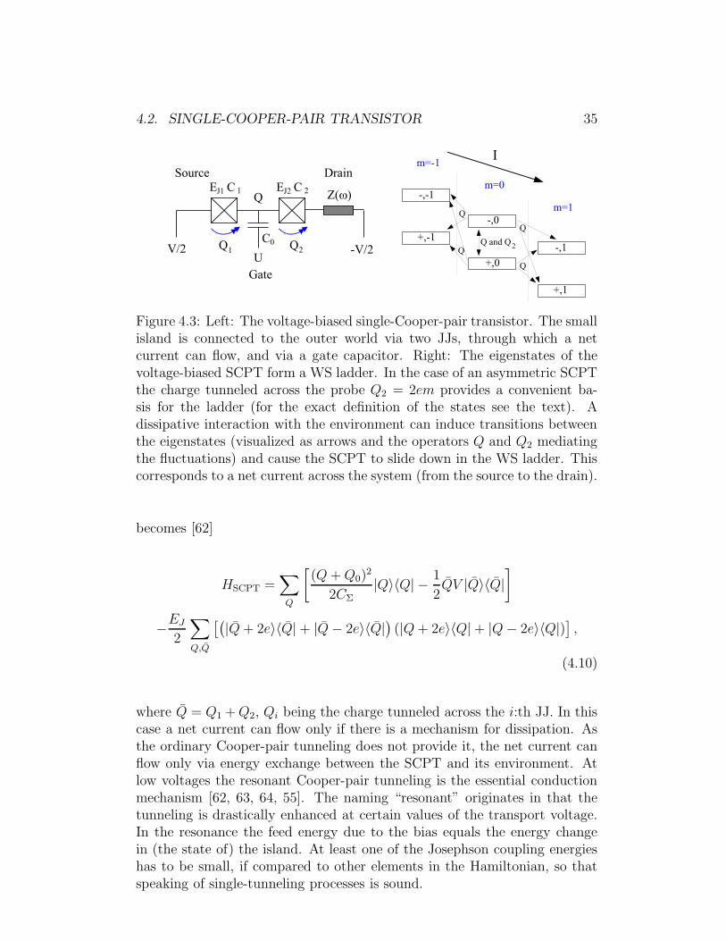
4.2. SINGLE-COOPER-PAIR TRANSISTOR 35
Figure 4.3: Left: The voltage-biased single-Cooper-pair transistor. The smallisland is connected to the outer world via two JJs, through which a netcurrent can flow, and via a gate capacitor. Right: The eigenstates of thevoltage-biased SCPT form a WS ladder. In the case of an asymmetric SCPTthe charge tunneled across the probe Q2 = 2em provides a convenient ba-sis for the ladder (for the exact definition of the states see the text). Adissipative interaction with the environment can induce transitions betweenthe eigenstates (visualized as arrows and the operators Q and Q2 mediatingthe fluctuations) and cause the SCPT to slide down in the WS ladder. Thiscorresponds to a net current across the system (from the source to the drain).
becomes [62]
HSCPT =∑
Q
[
(Q+Q0)2
2CΣ|Q〉〈Q| − 1
2QV |Q〉〈Q|
]
−EJ
2
∑
Q,Q
[(
|Q+ 2e〉〈Q| + |Q− 2e〉〈Q|)
(|Q+ 2e〉〈Q| + |Q− 2e〉〈Q|)]
,
(4.10)
where Q = Q1 +Q2, Qi being the charge tunneled across the i:th JJ. In thiscase a net current can flow only if there is a mechanism for dissipation. Asthe ordinary Cooper-pair tunneling does not provide it, the net current canflow only via energy exchange between the SCPT and its environment. Atlow voltages the resonant Cooper-pair tunneling is the essential conductionmechanism [62, 63, 64, 55]. The naming “resonant” originates in that thetunneling is drastically enhanced at certain values of the transport voltage.In the resonance the feed energy due to the bias equals the energy changein (the state of) the island. At least one of the Josephson coupling energieshas to be small, if compared to other elements in the Hamiltonian, so thatspeaking of single-tunneling processes is sound.
36 CHAPTER 4. APPLICATIONS
4.2.1 Resonant Cooper-pair tunneling
Papers II and III consider resonant tunneling of Cooper pairs across a voltage-biased SCPT. In a resonant process the island is excited as charge is trans-ported across the system, and vice versa. Irreversible processes can relaxthe excited state to a lower-energy one but in a way the charge originallytransported is not returned. Therefore the resonant tunneling leads to anet current with I − V peaks that can be related to the system’s energy-level structure, similarly as in Paper I. However, in Paper I we assumedthat the Cooper-pair tunneling across the small probe is incoherent due tofast interruption by the irreversible processes. In such a case the pertur-bative treatment of the probe is well valid. In Paper II we start from theopposite assumption and treat all the tunneling nonperturbatively and coher-ently. The decoherence is included perturbatively by using the Pauli-master-equation [31], where only diagonal elements (populations) of the density ma-trix are modeled. Paper III then gives a treatment that applies for arbitrarydecohering times. It also analyzes how different environments contribute tothe net current.
The nonperturbative calculation includes arbitrary-order Cooper-pair tun-neling across the JJs. The theoretical treatment can in many situations bereduced to a simple two-state system extended to a Wannier-Stark (WS)ladder [65, 66]. Which two eigenstates are selected in a single step dependson V and U . In the case of asymmetric SCPT the relevant states in a resonantsituation between the CPB’s ground and the first excited-state due to single-Cooper-pair tunneling across the probe are [E1(Q0) − E0(Q0) = 2eV , whereEi(Q0) are eigenenergies of the CPB]
|+, m〉 =1√2(|0〉|m〉 + |1〉|m+ 1〉) (4.11)
|−, m〉 =1√2(|0〉|m〉 − |1〉|m+ 1〉), (4.12)
where the states are expressed in the product basis of the CPB’s eigenstatesand the charge tunneled through the probe Q2 (2em). The correspondingeigenenergies are
E+m = −EJ2
2|〈1|e−iϕ|0〉| − 2eV m (4.13)
E−m = +EJ2
2|〈1|e−iϕ|0〉| − 2eV m. (4.14)
The eigenstates form a WS ladder with respect to m, i. e., a new eigenstate isobtained after a translationm→ m±1 with eigenenergy E → E∓2eV . If thesystem is closed, the states are steady and describe coherent superpositionsof the CPB’s eigenstates induced by coherent Cooper-pair tunneling acrossthe probe.
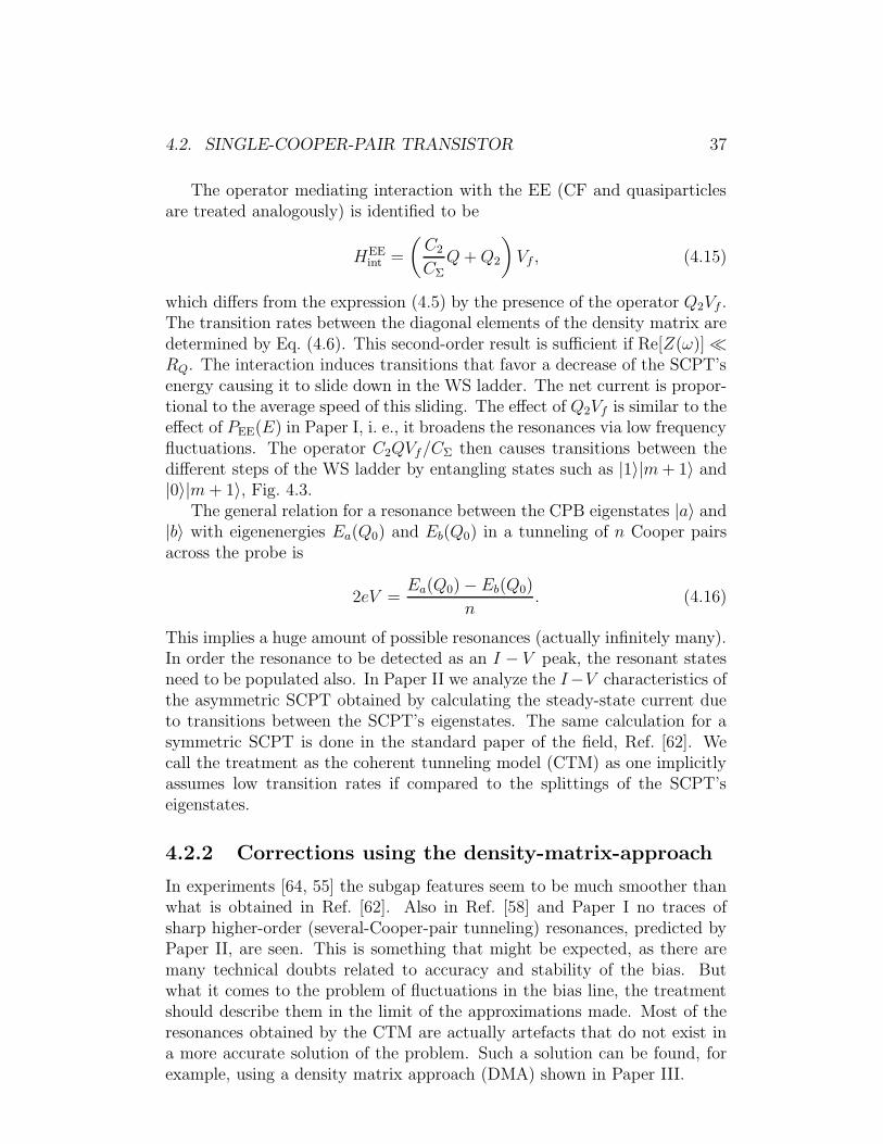
4.2. SINGLE-COOPER-PAIR TRANSISTOR 37
The operator mediating interaction with the EE (CF and quasiparticlesare treated analogously) is identified to be
HEEint =
(
C2
CΣQ+Q2
)
Vf , (4.15)
which differs from the expression (4.5) by the presence of the operator Q2Vf .The transition rates between the diagonal elements of the density matrix aredetermined by Eq. (4.6). This second-order result is sufficient if Re[Z(ω)] ≪RQ. The interaction induces transitions that favor a decrease of the SCPT’senergy causing it to slide down in the WS ladder. The net current is propor-tional to the average speed of this sliding. The effect of Q2Vf is similar to theeffect of PEE(E) in Paper I, i. e., it broadens the resonances via low frequencyfluctuations. The operator C2QVf/CΣ then causes transitions between thedifferent steps of the WS ladder by entangling states such as |1〉|m+ 1〉 and|0〉|m+ 1〉, Fig. 4.3.
The general relation for a resonance between the CPB eigenstates |a〉 and|b〉 with eigenenergies Ea(Q0) and Eb(Q0) in a tunneling of n Cooper pairsacross the probe is
2eV =Ea(Q0) − Eb(Q0)
n. (4.16)
This implies a huge amount of possible resonances (actually infinitely many).In order the resonance to be detected as an I − V peak, the resonant statesneed to be populated also. In Paper II we analyze the I−V characteristics ofthe asymmetric SCPT obtained by calculating the steady-state current dueto transitions between the SCPT’s eigenstates. The same calculation for asymmetric SCPT is done in the standard paper of the field, Ref. [62]. Wecall the treatment as the coherent tunneling model (CTM) as one implicitlyassumes low transition rates if compared to the splittings of the SCPT’seigenstates.
4.2.2 Corrections using the density-matrix-approach
In experiments [64, 55] the subgap features seem to be much smoother thanwhat is obtained in Ref. [62]. Also in Ref. [58] and Paper I no traces ofsharp higher-order (several-Cooper-pair tunneling) resonances, predicted byPaper II, are seen. This is something that might be expected, as there aremany technical doubts related to accuracy and stability of the bias. Butwhat it comes to the problem of fluctuations in the bias line, the treatmentshould describe them in the limit of the approximations made. Most of theresonances obtained by the CTM are actually artefacts that do not exist ina more accurate solution of the problem. Such a solution can be found, forexample, using a density matrix approach (DMA) shown in Paper III.
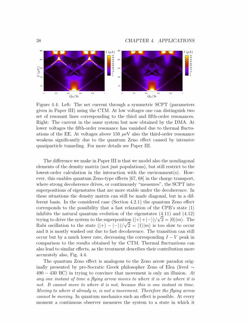
38 CHAPTER 4. APPLICATIONSV
(µV
)
Q0/2e
I (pA)
Q0/2e
I (pA)
Figure 4.4: Left: The net current through a symmetric SCPT (parametersgiven in Paper III) using the CTM. At low voltages one can distinguish twoset of resonant lines corresponding to the third and fifth-order resonances.Right: The current in the same system but now obtained by the DMA. Atlower voltages the fifth-order resonance has vanished due to thermal fluctu-ations of the EE. At voltages above 150 µeV also the third-order resonanceweakens significantly due to the quantum Zeno effect caused by intensivequasiparticle tunneling. For more details see Paper III.
The difference we make in Paper III is that we model also the nondiagonalelements of the density matrix (not just populations), but still restrict to thelowest-order calculation in the interaction with the environment(s). How-ever, this enables quantum Zeno-type effects [67, 68] in the charge transport,where strong decoherence drives, or continuously “measures”, the SCPT intosuperpositions of eigenstates that are more stable under the decoherence. Inthese situations the density matrix can still be made diagonal, but in a dif-ferent basis. In the considered case (Section 4.2.1) the quantum Zeno effectcorresponds to the possibility that a fast relaxation of the CPB’s state |1〉inhibits the natural quantum evolution of the eigenstates (4.11) and (4.12)trying to drive the system to the superposition (|+〉+|−〉)/
√2 = |0〉|m〉. The
Rabi oscillation to the state (|+〉 − |−〉)/√
2 = |1〉|m〉 is too slow to occurand it is mostly washed out due to fast decoherence. The transition can stilloccur but by a much lower rate, decreasing the corresponding I − V peak incomparison to the results obtained by the CTM. Thermal fluctuations canalso lead to similar effects, as the treatment describes their contribution moreaccurately also, Fig. 4.4.
The quantum Zeno effect is analogous to the Zeno arrow paradox orig-inally presented by pre-Socratic Greek philosopher Zeno of Elea (lived ∼490 − 430 BC) in trying to convince that movement is only an illusion. At
any one instant of time a flying arrow moves to where it is or to where it is
not. It cannot move to where it is not, because this is one instant in time.
Moving to where it already is, is not a movement. Therefore the flying arrow
cannot be moving. In quantum mechanics such an effect is possible. At everymoment a continuous observer measures the system to a state in which it
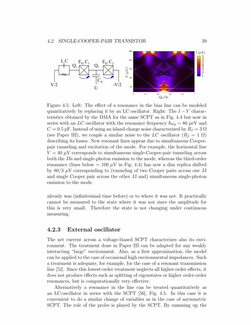
4.2. SINGLE-COOPER-PAIR TRANSISTOR 39
V(µ
V)
Q0/2e
I (pA)
Figure 4.5: Left: The effect of a resonance in the bias line can be modeledquantitatively by replacing it by an LC oscillator. Right: The I − V charac-teristics obtained by the DMA for the same SCPT as in Fig. 4.4 but now inseries with an LC oscillator with the resonance frequency ~ωp = 80 µeV andC = 0.5 pF. Instead of using an island-charge noise characterized by RI = 3 Ω(see Paper III), we couple a similar noise to the LC oscillator (Rf = 1 Ω)describing its losses. New resonant lines appear due to simultaneous Cooper-pair tunneling and excitation of the mode. For example, the horizontal lineV = 40 µV corresponds to simultaneous single-Cooper-pair tunneling acrossboth the JJs and single-photon emission to the mode, whereas the third-orderresonance (lines below ∼ 100 µV in Fig. 4.4) has now a dim replica shiftedby 80/3 µV corresponding to (tunneling of two Cooper pairs across one JJand single Cooper pair across the other JJ and) simultaneous single-photonemission to the mode.
already was (infinitesimal time before) or to where it was not. It practicallycannot be measured to the state where it was not since the amplitude forthis is very small. Therefore the state is not changing under continuousmeasuring.
4.2.3 External oscillator
The net current across a voltage-biased SCPT characterizes also its envi-ronment. The treatment done in Paper III can be adapted for any weaklyinteracting “large” environment. Also, as a first approximation, the modelcan be applied to the case of occasional high environmental impedances. Sucha treatment is adequate, for example, for the case of a resonant transmissionline [52]. Since this lowest-order treatment neglects all higher-order effects, itdoes not produce effects such as splitting of eigenstates or higher order-orderresonances, but is computationally very effective.
Alternatively a resonance in the line can be treated quantitatively asan LC-oscillator in series with the SCPT [56], Fig. 4.5. In this case it isconvenient to do a similar change of variables as in the case of asymmetricSCPT. The role of the probe is played by the SCPT. By summing up the
40 CHAPTER 4. APPLICATIONS
circuit’s electrical energies and using the Kirchhoff rules, the Hamiltonian canbe represented in the form H = HLC + HSCPT + HCC where the individualHamiltonians of the SCPT and the LC oscillator are separated and thenentangled capacitively by the term HCC. Under the assumption C ≫ CΣ =C1 +C2+C0, which is very reasonable since usually C1 ∼ 1 fF and C ∼ 1 pF,the operators are
HLC =(Ql − C12V )2
2C+ϕ2
l
2L(4.17)
HSCPT =(Qr + UC0)
2
2CΣ− V
2Q
−EJ1 cos(−ϕl + ϕr + ϕ) −EJ2 cos(−ϕr + ϕ) (4.18)
HCC =Ql(Qr + UC0)
2C, (4.19)
where C12 = C1/2 and we use the assumption C1 = C2, Ql (Qr) is theleft (right) island charge, a conjugated variable to ϕl (ϕr), and the sum ofthe charges tunneled across the JJs Q is a conjugated variable to ϕ. TheHamiltonian matrix is most efficiently written in the basis |l〉|Qr〉|Q〉 where|l〉 is an eigenstate of HLC with eigenenergy l~ωp = l~/
√LC. The excited
states of the oscillator correspond to different number of photons in the mode.The matrix elements 〈l|eiϕl|n〉 (l, n = 0, 1, 2 . . .) can be calculated analyticallyand describe excitation of the oscillator when tunneled charge flows into it.Referring to the last section of Paper III, the resonant structure in this casefollows the lines
eV =4EC
l + r
[
(l − r)2
2+
(
Q0
e+ n
)
(l − r)
]
+4∆
l + r− 2~ωp
l + r, (4.20)
some of which can be identified in Fig. 4.5.
4.3 Current-biased Josephson junction
The current-biased JJ is the device in which the macroscopic quantum-effectsof small JJs were first verified [5, 7, 6]. The phase difference across the JJwas shown to be able to quantum-mechanically tunnel across its potentialfield causing a voltage to appear across the JJ. This switching rate had aminimum value which the lowering of the temperature did not anymore affect.Today similar current-biased JJs are also good candidates for qubits [69] andmesoscopic amplifiers [70]. Their benefit is the immunity to the “island”charge fluctuations, but in larger JJs (qubits) also discrete fluctuators in theinsulating barriers start to exist (Section 3.2.3).
In the current-biased case the Hamiltonian of the JJ acquires an extraterm −~Iϕ/2e, which is the energy supplied by the current source I. The
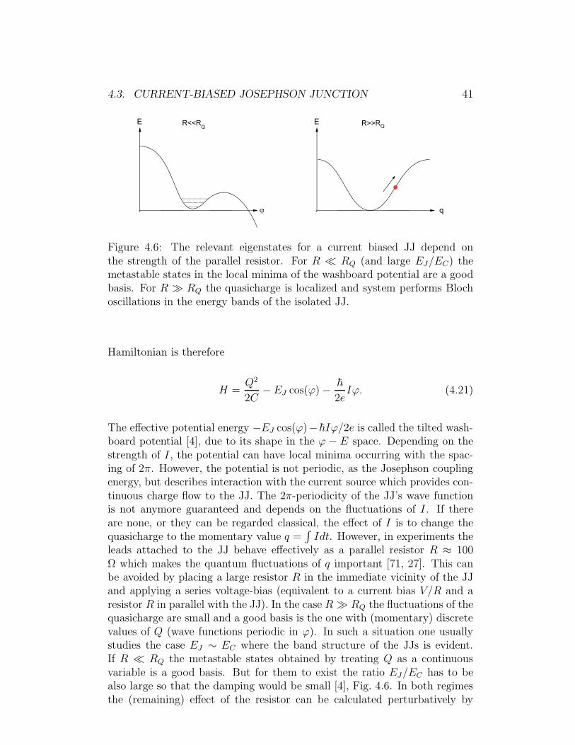
4.3. CURRENT-BIASED JOSEPHSON JUNCTION 41
Figure 4.6: The relevant eigenstates for a current biased JJ depend onthe strength of the parallel resistor. For R ≪ RQ (and large EJ/EC) themetastable states in the local minima of the washboard potential are a goodbasis. For R ≫ RQ the quasicharge is localized and system performs Blochoscillations in the energy bands of the isolated JJ.
Hamiltonian is therefore
H =Q2
2C− EJ cos(ϕ) − ~
2eIϕ. (4.21)
The effective potential energy −EJ cos(ϕ)−~Iϕ/2e is called the tilted wash-board potential [4], due to its shape in the ϕ − E space. Depending on thestrength of I, the potential can have local minima occurring with the spac-ing of 2π. However, the potential is not periodic, as the Josephson couplingenergy, but describes interaction with the current source which provides con-tinuous charge flow to the JJ. The 2π-periodicity of the JJ’s wave functionis not anymore guaranteed and depends on the fluctuations of I. If thereare none, or they can be regarded classical, the effect of I is to change thequasicharge to the momentary value q =
∫
Idt. However, in experiments theleads attached to the JJ behave effectively as a parallel resistor R ≈ 100Ω which makes the quantum fluctuations of q important [71, 27]. This canbe avoided by placing a large resistor R in the immediate vicinity of the JJand applying a series voltage-bias (equivalent to a current bias V/R and aresistor R in parallel with the JJ). In the case R ≫ RQ the fluctuations of thequasicharge are small and a good basis is the one with (momentary) discretevalues of Q (wave functions periodic in ϕ). In such a situation one usuallystudies the case EJ ∼ EC where the band structure of the JJs is evident.If R ≪ RQ the metastable states obtained by treating Q as a continuousvariable is a good basis. But for them to exist the ratio EJ/EC has to bealso large so that the damping would be small [4], Fig. 4.6. In both regimesthe (remaining) effect of the resistor can be calculated perturbatively by
42 CHAPTER 4. APPLICATIONS
decomposing I = Istatic + If and identifying
Hint = − ~
2eIfϕ, (4.22)
as the term mediating energy exchange between the current-biased JJ andthe dissipative environment. The environment is harmonic and can be rep-resented similarly as in the expressions (3.14-3.17).
4.3.1 Calculation scheme
In paper IV we consider a system where the current bias is provided by avoltage bias and a nearby resistor R ≫ RQ. This is equivalent to a currentbias V/R and a parallel R. Therefore the eigenstates of an isolated JJ arethe basis for our analysis. The effect of the parallel resistor is taken intoaccount perturbatively by using the density-matrix equation of motion inthe BM approximation (Section 3.1.3). For such a calculation we define ourbasis as |n, k〉 where n is a discrete parameter referring to the energy bandand k = q/2e a continuous parameter referring to the quasimomentum [71,72]. The states correspond to the eigenstates of the JJ’s Hamiltonian (withquasicharge q) and are normalized as
〈n, k|n′, k′〉 = δ(k′ − k)δn′,n. (4.23)
An arbitrary state is represented as |ψ〉 =∑
n
∫
dkψn(k)|n, k〉 and the densitymatrix as
ρ =∑
n1,n2
∫
dk1
∫
dk2ρn1n2(k1, k2)|n1, k1〉〈n2, k2|. (4.24)
When solving the density matrix’s equation of motion one needs to calculatematrix elements of ϕ which can be represented as
ϕnn′
kk′ = i∂
∂kδ(k − k′)δnn′ + ϕnn′
k δ(k − k′)(1 − δnn′) (4.25)
ϕnn′
k = −i⟨
n, k
∣
∣
∣
∣
∂
∂k
∣
∣
∣
∣
n′, k
⟩
. (4.26)
The first term in the r.h.s. of equation (4.25) describes intraband transitionswhereas the second term interband transitions. The element (4.26) is calcu-lated between the 2π-periodic parts of the wave functions and can be recastto the form
ϕnn′
k = −i
⟨
n, k∣
∣
∣
2eQCΣ
∣
∣
∣n′, k
⟩
En(k) − En′(k), (4.27)
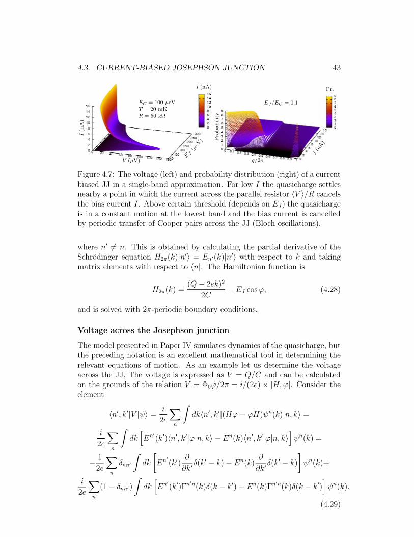
4.3. CURRENT-BIASED JOSEPHSON JUNCTION 43
I(n
A)
V (µV)
I (nA)
E J(µ
eV)
EC = 100 µeVT = 20 mKR = 50 kΩ
Pro
bability
q/2e
Pr.
I(n
A)
EJ/EC = 0.1
Figure 4.7: The voltage (left) and probability distribution (right) of a currentbiased JJ in a single-band approximation. For low I the quasicharge settlesnearby a point in which the current across the parallel resistor 〈V 〉/R cancelsthe bias current I. Above certain threshold (depends on EJ) the quasichargeis in a constant motion at the lowest band and the bias current is cancelledby periodic transfer of Cooper pairs across the JJ (Bloch oscillations).
where n′ 6= n. This is obtained by calculating the partial derivative of theSchrodinger equation H2π(k)|n′〉 = En′(k)|n′〉 with respect to k and takingmatrix elements with respect to 〈n|. The Hamiltonian function is
H2π(k) =(Q− 2ek)2
2C−EJ cosϕ, (4.28)
and is solved with 2π-periodic boundary conditions.
Voltage across the Josephson junction
The model presented in Paper IV simulates dynamics of the quasicharge, butthe preceding notation is an excellent mathematical tool in determining therelevant equations of motion. As an example let us determine the voltageacross the JJ. The voltage is expressed as V = Q/C and can be calculatedon the grounds of the relation V = Φ0ϕ/2π = i/(2e) × [H,ϕ]. Consider theelement
〈n′, k′|V |ψ〉 =i
2e
∑
n
∫
dk〈n′, k′|(Hϕ− ϕH)ψn(k)|n, k〉 =
i
2e
∑
n
∫
dk[
En′
(k′)〈n′, k′|ϕ|n, k〉 −En(k)〈n′, k′|ϕ|n, k〉]
ψn(k) =
− 1
2e
∑
n
δnn′
∫
dk
[
En′
(k′)∂
∂k′δ(k′ − k) − En(k)
∂
∂k′δ(k′ − k)
]
ψn(k)+
i
2e
∑
n
(1 − δnn′)
∫
dk[
En′
(k′)Γn′n(k)δ(k − k′) −En(k)Γn′n(k)δ(k − k′)]
ψn(k).
(4.29)
44 CHAPTER 4. APPLICATIONS
For the next expression we use the relation ∂∂k′ δ(k
′ − k) = − ∂∂kδ(k′ − k), do
integration by parts with respect to k, use the fact that the substitutionalterms vanish (periodic system) and obtain
〈n′, k′|V |ψ〉 =δnn′
2eE ′(k′)ψn′
(k′) +i
2e
∑
n 6=n′
[En′
(k′) −En(k′)]Γn′n(k′)ψn′
(k′)
.
(4.30)
In the case the original state is a pure Bloch state |m, k0〉 =∫
dkδ(k−k0)|n, k〉one obtains
〈n′, k′|V |n, k0〉 =δnn′
2eE ′(k′)δ(k′ − k0)
+i
2e(1 − δnn′)[En′
(k′) − En(k′)]Γn′n(k′)δ(k′ − k0). (4.31)
The elements are diagonal with respect to quasimomentum. If we can restrictto considering only such diagonal elements, the normalisation δ(k′ − k0) canbe neglected (cancels out in the equations) and one obtains by marking k0 = kthat
〈n′, k|V |n, k〉 =δnn′
2eE ′(k) +
i
2e(1 − δnn′)[En′
(k) −En(k)]Γn′n(k). (4.32)
One sees that the Bloch state’s expectation value for the voltage is propor-tional to E ′(k) and that superpositions produce terms proportional to theZener-tunneling amplitude. In Fig. 4.7 we show results for the steady statevoltage and probability distribution (in k-space) as a function of the biascurrent I. The simulations are based on Eq. (4.32) and the equations foundin Paper IV.
4.3.2 Probing energy-band dynamics
Paper IV considers probing of energy-band dynamics in a current-biasedJJ using a small JJ. The circuit can be also seen as the Bloch-oscillatingtransistor [70, 73, 74] (BOT) with JJ at the base. The BOT is analogous tothe bipolar transistor in which the base current controls the current betweenthe emitter and the collector, Fig. 4.8. Alternatively, the system can also beseen as a SCPT in which the gate capacitor is replaced by a large resistorR and therefore by a dynamic polarisation charge q. The idea in PaperIV is that for certain voltages Vb and V the small base JJ induces (extra)transitions between the system’s energy bands and enhances the net currentacross the base. Therefore the base current probes the system’s energy-bandstructure and quasicharge dynamics.
The equivalent current-biased circuit is shown in Fig. 4.8 (right). Herewe have placed the bias in parallel with the emitter JJ, which is assumed to
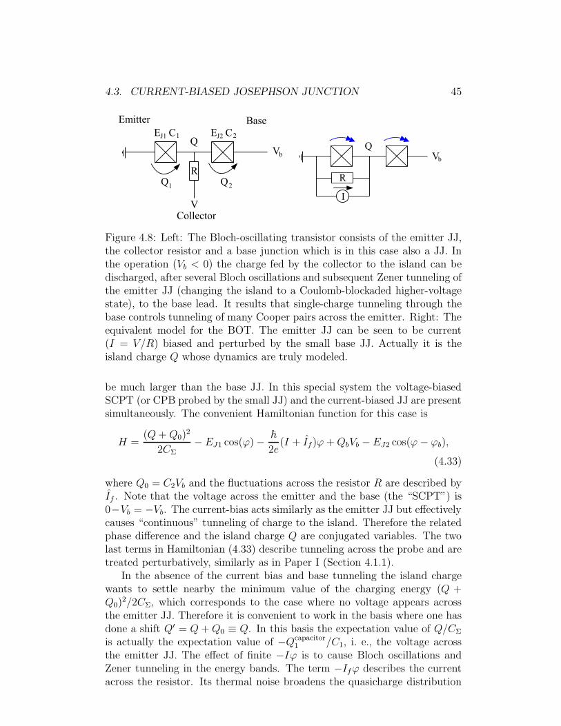
4.3. CURRENT-BIASED JOSEPHSON JUNCTION 45
Figure 4.8: Left: The Bloch-oscillating transistor consists of the emitter JJ,the collector resistor and a base junction which is in this case also a JJ. Inthe operation (Vb < 0) the charge fed by the collector to the island can bedischarged, after several Bloch oscillations and subsequent Zener tunneling ofthe emitter JJ (changing the island to a Coulomb-blockaded higher-voltagestate), to the base lead. It results that single-charge tunneling through thebase controls tunneling of many Cooper pairs across the emitter. Right: Theequivalent model for the BOT. The emitter JJ can be seen to be current(I = V/R) biased and perturbed by the small base JJ. Actually it is theisland charge Q whose dynamics are truly modeled.
be much larger than the base JJ. In this special system the voltage-biasedSCPT (or CPB probed by the small JJ) and the current-biased JJ are presentsimultaneously. The convenient Hamiltonian function for this case is
H =(Q+Q0)
2
2CΣ− EJ1 cos(ϕ) − ~
2e(I + If)ϕ+QbVb − EJ2 cos(ϕ− ϕb),
(4.33)
where Q0 = C2Vb and the fluctuations across the resistor R are described byIf . Note that the voltage across the emitter and the base (the “SCPT”) is0−Vb = −Vb. The current-bias acts similarly as the emitter JJ but effectivelycauses “continuous” tunneling of charge to the island. Therefore the relatedphase difference and the island charge Q are conjugated variables. The twolast terms in Hamiltonian (4.33) describe tunneling across the probe and aretreated perturbatively, similarly as in Paper I (Section 4.1.1).
In the absence of the current bias and base tunneling the island chargewants to settle nearby the minimum value of the charging energy (Q +Q0)
2/2CΣ, which corresponds to the case where no voltage appears acrossthe emitter JJ. Therefore it is convenient to work in the basis where one hasdone a shift Q′ = Q+Q0 ≡ Q. In this basis the expectation value of Q/CΣ
is actually the expectation value of −Qcapacitor1 /C1, i. e., the voltage across
the emitter JJ. The effect of finite −Iϕ is to cause Bloch oscillations andZener tunneling in the energy bands. The term −Ifϕ describes the currentacross the resistor. Its thermal noise broadens the quasicharge distribution
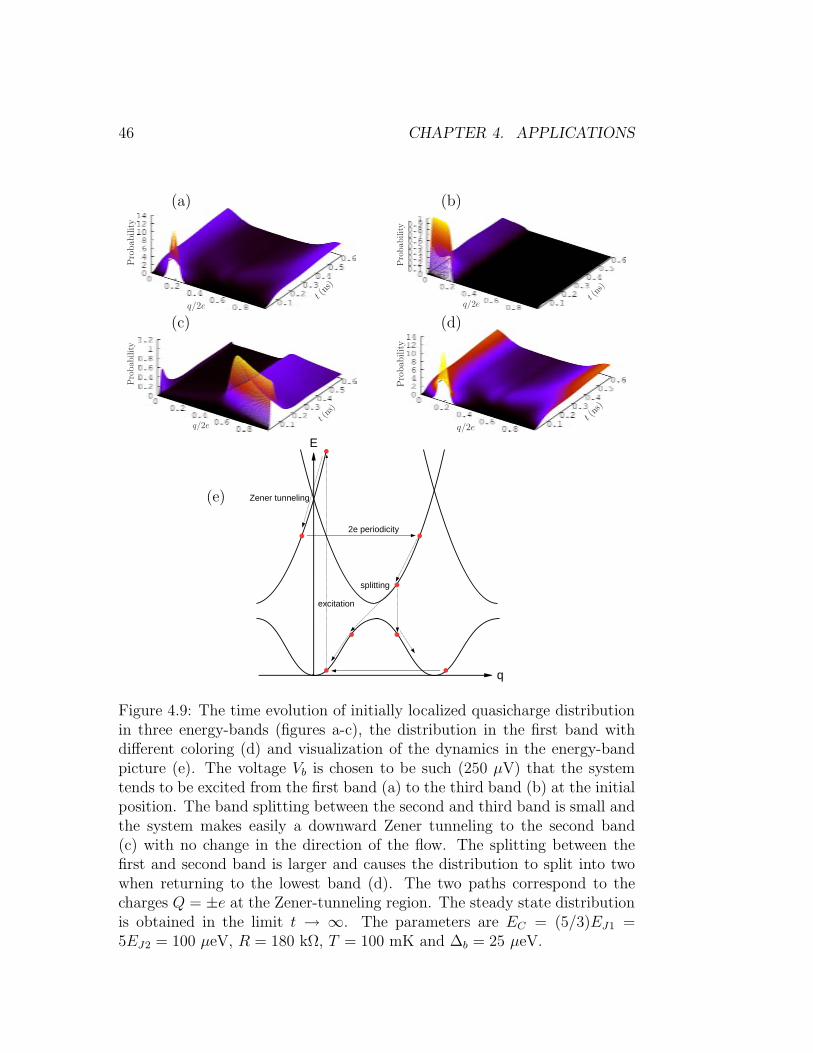
46 CHAPTER 4. APPLICATIONSP
robab
ility
q/2et(n
s)
(a)
Pro
bab
ility
q/2et(n
s)
(b)
Pro
bab
ility
q/2et(n
s)
(c)
Pro
bab
ility
q/2et(n
s)
(d)
(e)
Figure 4.9: The time evolution of initially localized quasicharge distributionin three energy-bands (figures a-c), the distribution in the first band withdifferent coloring (d) and visualization of the dynamics in the energy-bandpicture (e). The voltage Vb is chosen to be such (250 µV) that the systemtends to be excited from the first band (a) to the third band (b) at the initialposition. The band splitting between the second and third band is small andthe system makes easily a downward Zener tunneling to the second band(c) with no change in the direction of the flow. The splitting between thefirst and second band is larger and causes the distribution to split into twowhen returning to the lowest band (d). The two paths correspond to thecharges Q = ±e at the Zener-tunneling region. The steady state distributionis obtained in the limit t → ∞. The parameters are EC = (5/3)EJ1 =5EJ2 = 100 µeV, R = 180 kΩ, T = 100 mK and ∆b = 25 µeV.
4.3. CURRENT-BIASED JOSEPHSON JUNCTION 47
and quantum noise results in incoherent current ∼ Q/CΣR.The presence of base tunneling can excite the system to higher bands
from which the system returns to lower bands by “sliding” down the energybands and making downward Zener transitions nearby the points of minimumsplitting. The sliding correspond to charging of the island via the collectorcurrent and its speed is proportional to the voltage across the resistor. Suchan effect is visualized in Fig. 4.9, where the real-time dynamics are plottedstarting from a narrow Gaussian distribution at k ∼ 0.2. Such resonantprocesses contribute as peaks in the Ib − Vb characteristics.
Numerical modeling
The steady-state distribution of all the quasicharge dynamics is a solution ofthe discretized matrix-equation, derived in Paper IV. The equation has beengreatly simplified by considering only diagonal states in q (the approximationholds in the case R ≫ RQ). Still, it is important to discretize the quasichargespace much denser than typical changes occur in the corresponding energy-eigenstates. For small band-splittings this becomes a problem as changesoccur rapidly nearby k = 0 or k = 1/2, see Fig. 2.4. Therefore, in manycases the calculation is still quite challenging and needs to be solved with anappropriate method.
A numerically effective algorithm takes into account that only transitionsbetween the nearby states of the quasicharge exist. This results in a block-tridiagonal matrix-equation for the steady state of the system, which hasthen its own effective inversion algorithm (Thomas algorithm). The upper-right and the lower-left corners of the matrix equation have still nonvanishingelements, which are not present in the block-tridiagonal form, but their effectcan be included by using the Woodbury matrix identity. When using generalalgorithms the computational limits occurred nearby n ∼ 500 in three-bandsimulations, whereas in the case of the block-tridiagonal algorithm the limitwas nearby n ∼ 30000. After that it was the the numerical error that madethe algorithm out of use. Indeed, Fig. 2 in Paper IV includes an effect oftoo wide discretization, as the Zener-tunneling region is separated into twodifferent regions. The origin of this separation is the Bloch oscillations inthe second band, which reduce the base current and result in the observeddip between the pointed regions. Such oscillations was later shown to bean artefact of too wide discretization. In the more accurate simulations theZener-tunneling region is uniform as the dip is enhanced to the level of thetwo maxima.
Quasiparticle tunneling
To model quasiparticle tunneling across the JJs we proceed similarly as inPaper III. Assuming that the interaction with quasiparticles can be modeled
48 CHAPTER 4. APPLICATIONS
by the lowest-order expansion of the density-matrix’s equation of motion(RT > RQ), one obtains that the relevant operator describing the transitionsis
T =∑
Q
|Q− e〉〈Q|, (4.34)
and that quasiparticles are traced into the effective damping functionD+q (ω) ≡
Dq(ω), Eq. (3.39). In the case of the base JJ the quasiparticle tunnelingand simultaneous transition |ni, ki〉 → |n, kf〉 releases/absorbs the energy~ωni(ki) − ~ωnf (kf) − eVb. Using the notation
〈n′, k′|T |n, k〉 = Tn′n(k′)δ(k′ − k +1
2) (4.35)
〈n′, k′|T †|n, k〉 = T ∗nn′(k)δ(k′ − k − 1
2), (4.36)
one can calculate the terms originating in the positive-direction tunneling(T -operator)
ρnn′
qp (k) =1
~2
∑
ni,n′i
ρnin′i
(
k +1
2, k +
1
2
)
Tnni(k)T ∗n′n′
i(k)×
Dq
[
ωni
(
k +1
2
)
− ωnf (k) − eVb
~
]
+Dq
[
ωn′i
(
k +1
2
)
− ωn′f (k) − eVb
~
]
,
(4.37)
which can also be seen as the “type 1” diagrams in the language of theAppendix in Paper III. The type 2 diagrams give the contribution
ρnn′
qp (k) = − 1
~2
∑
ni,nv
ρnin′
(k)Tnvni
(
k +1
2
)
T ∗nvn
(
k +1
2
)
×
Dq
[
ωni(k) − ωnv
(
k +1
2
)
− eVb
~
]
, (4.38)
and the mirror diagram
ρnn′
qp (k) = − 1
~2
∑
n′i,nv
ρn,n′i (k)T ∗nvn′
i
(
k +1
2
)
Tnvn′
(
k +1
2
)
×
Dq
[
ωn′i(k) − ωnv
(
k +1
2
)
− eVb
~
]
. (4.39)
The opposite direction tunneling is obtained by the change T → T † andeVb → −eVb. For the tunneling across the emitter JJ the automatic workterm ±eVb is set to zero and in Eq. (3.39) one uses the emitter quasiparticle-current Iss(~ω/e) (instead of the base current).
4.3. CURRENT-BIASED JOSEPHSON JUNCTION 49
Improvements for the Cooper-pair tunneling rates
The Cooper-pair tunneling across the emitter is treated exactly but across thebase perturbatively. In Paper IV we introduce the transition rates betweenthe eigenstates due to the base tunneling as a Lorentzian function (4.7).This is a sufficient treatment for small EJ2. For a qualitative description ofmoderate EJ2 we should improve this approximation by two ways. First, theprobability that the environment emits (rather than absorbs) the energy Eduring the Cooper-pair tunneling is damped by exp(−E/kBT ) [16]. Such aneffect brings changes to the supercurrent region, i. e., for processes wherecharge is transported across the system with no change in the state of theisland. The “supercurrent” occurs here via incoherent Cooper-pair tunnelingand leads to the phase-diffusion branch in the low-voltage part of the I − Vcharacteristics [53]. The second improvement we can make is to take intoaccount the possible nondiagonality of the island’s density matrix. In analogyto what is done in the DMA in Paper III, we can model also transitionsbetween arbitrary nondiagonal elements of the density matrix. As the relateddamping function (describing the effect of the base’s environment) we usethe transition rate function (4.7) and consider only diagonal states in thetunneled charge Q2. Further, Lindblad approximation of the perturbation(by redefining some of the nondiagonal transition rates) can be taken forlarge values of EJ2 in order to ensure the positivity of the density matrix,see Paper III. In this case the current across the base (in the second-orderapproximation) is a sum of the contributions
I = 2e∑
nin′ink
Re[
ρssnin′
i(k)Γni→n
n′i→n(k)
]
, (4.40)
where ρss(k) is the steady-state density-matrix and Γ the generalized transition-rate tensor due to Cooper-pair tunneling across the base JJ. Positive directionterms are summed with positive signs and the negative direction terms withnegative signs. The quasiparticle current across the base JJ is calculatedsimilarly. The average current from the collector to the island is deduced tobe [71, 72]
Ic = I +〈Qcapacitor
1 /C1〉R
=V
R− 〈Q/CΣ〉
R, (4.41)
and the emitter current follows from the relation IE = IR + IC .
4.3.3 Model for the Bloch-oscillating transistor
The model presented in Paper IV, with the supplements given in Section4.3.2, can be used for modeling the steady-state properties of the BOT. TheBOT is designed to work as an amplifier for the base current and therefore in
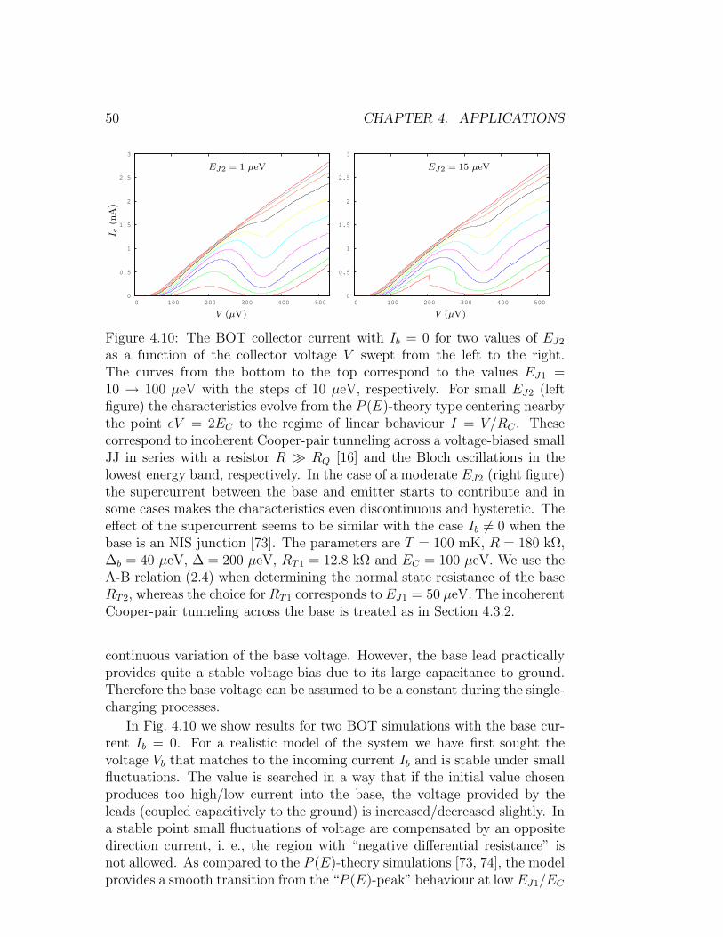
50 CHAPTER 4. APPLICATIONS
0
0.5
1
1.5
2
2.5
3
0 100 200 300 400 500
I c(n
A)
V (µV)
EJ2 = 1 µeV
0
0.5
1
1.5
2
2.5
3
0 100 200 300 400 500
V (µV)
EJ2 = 15 µeV
Figure 4.10: The BOT collector current with Ib = 0 for two values of EJ2
as a function of the collector voltage V swept from the left to the right.The curves from the bottom to the top correspond to the values EJ1 =10 → 100 µeV with the steps of 10 µeV, respectively. For small EJ2 (leftfigure) the characteristics evolve from the P (E)-theory type centering nearbythe point eV = 2EC to the regime of linear behaviour I = V/RC . Thesecorrespond to incoherent Cooper-pair tunneling across a voltage-biased smallJJ in series with a resistor R ≫ RQ [16] and the Bloch oscillations in thelowest energy band, respectively. In the case of a moderate EJ2 (right figure)the supercurrent between the base and emitter starts to contribute and insome cases makes the characteristics even discontinuous and hysteretic. Theeffect of the supercurrent seems to be similar with the case Ib 6= 0 when thebase is an NIS junction [73]. The parameters are T = 100 mK, R = 180 kΩ,∆b = 40 µeV, ∆ = 200 µeV, RT1 = 12.8 kΩ and EC = 100 µeV. We use theA-B relation (2.4) when determining the normal state resistance of the baseRT2, whereas the choice for RT1 corresponds to EJ1 = 50 µeV. The incoherentCooper-pair tunneling across the base is treated as in Section 4.3.2.
continuous variation of the base voltage. However, the base lead practicallyprovides quite a stable voltage-bias due to its large capacitance to ground.Therefore the base voltage can be assumed to be a constant during the single-charging processes.
In Fig. 4.10 we show results for two BOT simulations with the base cur-rent Ib = 0. For a realistic model of the system we have first sought thevoltage Vb that matches to the incoming current Ib and is stable under smallfluctuations. The value is searched in a way that if the initial value chosenproduces too high/low current into the base, the voltage provided by theleads (coupled capacitively to the ground) is increased/decreased slightly. Ina stable point small fluctuations of voltage are compensated by an oppositedirection current, i. e., the region with “negative differential resistance” isnot allowed. As compared to the P (E)-theory simulations [73, 74], the modelprovides a smooth transition from the “P (E)-peak” behaviour at low EJ1/EC
4.3. CURRENT-BIASED JOSEPHSON JUNCTION 51
to almost linear behaviour at large EJ1/EC . We also observe hysteresis, evenfor Ib = 0, due to the presence of the supercurrent. Both the observationsare in qualitative agreement with recent experimental studies for the BOTwith SIS junction at the base [75]. More detailed investigation is going to bepublished elsewhere.

52 CHAPTER 4. APPLICATIONS
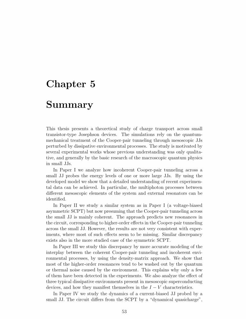
Chapter 5
Summary
This thesis presents a theoretical study of charge transport across smalltransistor-type Josephson devices. The simulations rely on the quantum-mechanical treatment of the Cooper-pair tunneling through mesoscopic JJsperturbed by dissipative environmental processes. The study is motivated byseveral experimental works whose previous understanding was only qualita-tive, and generally by the basic research of the macroscopic quantum physicsin small JJs.
In Paper I we analyze how incoherent Cooper-pair tunneling across asmall JJ probes the energy levels of one or more large JJs. By using thedeveloped model we show that a detailed understanding of recent experimen-tal data can be achieved. In particular, the multiphoton processes betweendifferent mesoscopic elements of the system and external resonators can beidentified.
In Paper II we study a similar system as in Paper I (a voltage-biasedasymmetric SCPT) but now presuming that the Cooper-pair tunneling acrossthe small JJ is mainly coherent. The approach predicts new resonances inthe circuit, corresponding to higher-order effects in the Cooper-pair tunnelingacross the small JJ. However, the results are not very consistent with exper-iments, where most of such effects seem to be missing. Similar discrepancyexists also in the more studied case of the symmetric SCPT.
In Paper III we study this discrepancy by more accurate modeling of theinterplay between the coherent Cooper-pair tunneling and incoherent envi-ronmental processes, by using the density-matrix approach. We show thatmost of the higher-order resonances tend to be washed out by the quantumor thermal noise caused by the environment. This explains why only a fewof them have been detected in the experiments. We also analyze the effect ofthree typical dissipative environments present in mesoscopic superconductingdevices, and how they manifest themselves in the I − V characteristics.
In Paper IV we study the dynamics of a current-biased JJ probed by asmall JJ. The circuit differs from the SCPT by a “dynamical quasicharge”,
53
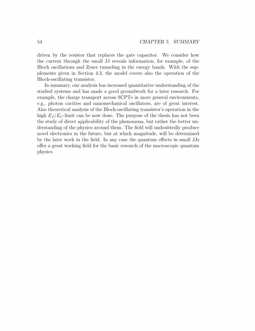
54 CHAPTER 5. SUMMARY
driven by the resistor that replaces the gate capacitor. We consider howthe current through the small JJ reveals information, for example, of theBloch oscillations and Zener tunneling in the energy bands. With the sup-plements given in Section 4.3, the model covers also the operation of theBloch-oscillating transistor.
In summary, our analysis has increased quantitative understanding of thestudied systems and has made a good groundwork for a later research. Forexample, the charge transport across SCPTs in more general environments,e.g., photon cavities and nanomechanical oscillators, are of great interest.Also theoretical analysis of the Bloch-oscillating transistor’s operation in thehigh EJ/EC-limit can be now done. The purpose of the thesis has not beenthe study of direct applicability of the phenomena, but rather the better un-derstanding of the physics around them. The field will undoubtedly producenovel electronics in the future, but at which magnitude, will be determinedby the later work in the field. In any case the quantum effects in small JJsoffer a great working field for the basic research of the macroscopic quantumphysics.
Bibliography
[1] J. Clarke and F. K. Wilhelm, Nature (London) 453, 1031 (2008).
[2] B. D. Josephson, Phys. Lett. 1, 251 (1962).
[3] P. W. Anderson and J. M. Rowell, Phys. Rev. Lett. 10, 230 (1963).
[4] M. Tinkham, Introduction to Superconductivity, 2nd ed. (McGraw-Hill,New York, 1996).
[5] R. F. Voss and R. A. Webb, Phys. Rev. Lett. 47, 265 (1981).
[6] M. H. Devoret, J. M. Martinis, and J. Clarke, Phys. Rev. Lett. 55, 1908(1985).
[7] J. M. Martinis, M. H. Devoret, and J. Clarke, Phys. Rev. Lett. 55, 1543(1985).
[8] Y. Nakamura, C. D. Chen, and J. S. Tsai, Phys. Rev. Lett. 79, 2328(1997).
[9] Y. Nakamura, Yu. A. Pashkin, and J. S. Tsai, Nature (London) 398,786 (1999).
[10] A. Naik, O. Buu, M. D. LaHaye, A. D. Armour, A. A. Clerk,M. P. Blencowe, and K. C. Schwab, Nature (London) 443, 193 (2006).
[11] A. Wallraff, D. I. Schuster, A. Blais, L. Frunzio, R.-S. Huang, J. Majer,S. Kumar, S. M. Girvin and R. J. Schoelkopf, Nature (London) 431,162 (2004).
[12] D. Gunnarsson, J. Tuorila, A. Paila, J. Sarkar, E. Thuneberg,Y. Makhlin, and P. Hakonen, Phys. Rev. Lett. 101, 256806 (2008).
[13] Yu. Makhlin, G. Schon, and A. Shnirman, Rev. Mod. Phys. 73, 357(2001).
[14] G. Wendin and V. S. Shumeiko, Low Temp. Phys. 33, 724 (2007).
55
56 BIBLIOGRAPHY
[15] G. Ithier, E. Collin, P. Joyez, P. J. Meeson, D. Vion, D. Esteve,F. Chiarello, A. Shnirman, Y. Makhlin, J. Schriefl, and G. Schon, Phys.Rev. B 72, 134519 (2005).
[16] G.-L. Ingold and Yu. V. Nazarov, in Single Charge Tunneling: Coulomb
Blockade Phenomena in Nanostructures, edited by H. Grabert andM. H. Devoret (Plenum, New York, 1992), p. 21.
[17] M. A. Sillanpaa, L. Roschier, and P. J. Hakonen, Phys. Rev. Lett. 93,066805 (2004).
[18] J. M. Kivioja, T. E. Nieminen, J. Claudon, O. Buisson,F. W. J. Hekking, and J. P. Pekola, New J. Phys. 7, 179 (2005).
[19] E. B. Sonin, J. Low Temp. Phys. 146, 161 (2007).
[20] M. Schlosshauer, Rev. Mod. Phys. 76, 1267 (2004).
[21] R. P. Feynman, R. B. Leighton, and M. Sands, The Feynman Lectures
on Physics, Vol. 3 (Addison-Wesley, Reading, MA, 1965), chapter 21.
[22] J. Bardeen, L. N. Cooper, and J. R. Schrieffer, Phys. Rev. 108, 1175(1957).
[23] J. W. Wilkins, in Tunneling Phenomena in Solids, edited by E. Burn-stein and S. Lundqvist (Plenum, New York, 1969), p. 333.
[24] J. M. Martinis and K. Osbourne, in Quantum Entanglement and In-
formation Processing, Proceedings of the Les Houches Summer School2003, (Les Houches, Volume session LXXIX) edited by D. Esteve, J.-M. Raimond, and J. Dalibard, (Elsevier, 2004). Cond-mat/0402415.
[25] K. K. Likharev, Dynamics of Josephson Junctions and Circuits (OPA,Amsterdam, 1986).
[26] V. Ambegaokar and A. Baratoff, Phys. Rev. Lett. 10, 486 (1963).
[27] G. Schon and A. D. Zaikin, Phys. Rep. 198, 237 (1990).
[28] P. Carruthers and M. M. Nieto, Rev. Mod. Phys. 40, 411 (1968).
[29] D. V. Averin, Fortschr. Phys. 48, 1055 (2000).
[30] A. O. Caldeira and A. J. Leggett, Ann. Phys. (N.Y.) 149, 374 (1983).
[31] U. Weiss, Quantum Dissipative Systems, 2nd ed. (World Scientific, Sin-gapore, 1999).
BIBLIOGRAPHY 57
[32] R. P. Feynman and A. R. Hibbs, Quantum Mechanics and Path Integrals,(McGraw-Hill, New York, 1965).
[33] R. P. Feynman, Statistical Mechanics, (Westview Press, 1998).
[34] R. P. Feynman and F. L. Vernon, Ann. Phys. (N.Y.) 24, 118 (1963).
[35] H. Schoeller and G. Schon, Phys. Rev. B 50, 18436 (1994).
[36] Yu. Makhlin, G. Schon, and A. Shnirman, in Exploring the Quantum-
Classical Frontier, edited by J. R. Friedman and S. Han (Nova Science,Commack, NY, 2002), p. 405. Cond-mat/9811029
[37] B. Kubala, G. Johansson, and J. Konig, Phys. Rev. B 73, 165316 (2006).
[38] G. C. Wick, Phys. Rev. 80, 268 (1950).
[39] T. Ojanen and T. T. Heikkila, Phys. Rev. B 73, 020501(R) (2006).
[40] G. Lindblad, Commun. Math. Phys. 48, 119 (1976).
[41] S. M. Barnett and S. Stenholm, Phys. Rev. A 64, 033808 (2001).
[42] S. Maniscalco and F. Petruccione, Phys. Rev. A 73, 012111 (2006).
[43] Y. Nakamura, Yu. A. Pashkin, T. Yamamoto, and J. S. Tsai, Phys. Rev.Lett. 88, 047901 (2002).
[44] O. Astafiev, Yu. A. Pashkin, Y. Nakamura, T. Yamamoto, and J. S. Tsai,Phys. Rev. Lett. 93, 267007 (2004).
[45] R. W. Simmonds, K. M. Lang, D. A. Hite, S. Nam, D. P. Pappas, andJ. M. Martinis, Phys. Rev. Lett. 93, 077003 (2004).
[46] P. Dutta and P. M. Horn, Rev. Mod. Phys. 53, 497 (1981).
[47] A. Shnirman, G. Schon, I. Martin, and Yu. Makhlin, Phys. Rev. Lett.94, 127002 (2005).
[48] L. Faoro, J. Bergli, B. L. Altshuler, and Y. M. Galperin, Phys. Rev.Lett. 95, 046805 (2005).
[49] D. J. van Harlingen, T. L. Robertson, B. L. T. Plourde, P. A. Reichardt,T. A. Crane, and J. Clarke, Phys. Rev. B 70, 064517 (2004).
[50] J. M. Martinis, K. B. Cooper, R. McDermott, M. Steffen, M. Ansmann,K. D. Osborn, K. Cicak, S. Oh, D. P. Pappas, R. W. Simmonds, andC. C. Yu, Phys. Rev. Lett. 95, 210503 (2005).
58 BIBLIOGRAPHY
[51] H. B. Callen and T. A. Welton, Phys. Rev. 83, 34 (1951).
[52] T. Holst, D. Esteve, C. Urbina, and M. H. Devoret, Phys. Rev. Lett.73, 3455 (1994).
[53] G.-L. Ingold, H. Grabert, and U. Eberhardt, Phys. Rev. B 50, 395(1994).
[54] M. H. Devoret, in Fluctuations Quantiques, (Elsevier Science, 1997),p.351.
[55] P. Joyez, Ph.D. thesis, Paris 6 University, 1995.
[56] D. M. Pozar Microwave Engineering, 3rd ed. (Wiley, Hoboken, NJ,2005).
[57] J. A. Schreier, A. A. Houck, J. Koch, D. I. Schuster, B. R. Johnson,J. M. Chow, J. M. Gambetta, J. Majer, L. Frunzio, M. H. Devoret,S. M. Girvin, and R. J. Schoelkopf, Phys. Rev. B 77, 180502(R) (2008).
[58] R. Lindell, J. Penttila, M. Sillanpaa, and P. Hakonen, Phys. Rev. B 68,052506 (2003).
[59] F. W. J. Hekking, and Yu. V. Nazarov, Phys. Rev. B 49, 6847 (1994).
[60] A. A. Clerk, S. M. Girvin, A. K. Nguyen, and A. D. Stone, Phys. Rev.Lett. 89, 176804 (2002).
[61] D. Vion, A. Aassime, A. Cottet, P. Joyez, H. Pothier, C. Urbina, D. Es-teve, and M. H. Devoret, Science 296, 886 (2002).
[62] A. Maassen van den Brink, A. A. Odintsov, P. A. Bobbert, and G. Schon,Z. Phys. B: Condens. Matter 85, 459 (1991).
[63] A. Maassen van den Brink, G. Schon, and L. J. Geerligs, Phys. Rev.Lett. 67, 3030 (1991).
[64] D. B. Haviland, Y. Harada, P. Delsing, C. D. Chen, and T. Claeson,Phys. Rev. Lett. 73, 1541 (1994).
[65] G. H. Wannier, Phys. Rev. 117, 432 (1960).
[66] See for example: E. E. Mendez and G. Bastard, Phys. Today 46, 34(1993).
[67] R. Harris and L. Stodolsky, Phys. Lett. B 116, 464 (1982).
[68] A. Shnirman and Yu. Makhlin, JETP. Lett. 78, 447 (2003).
BIBLIOGRAPHY 59
[69] J. M. Martinis, S. Nam, J. Aumentado, and C. Urbina, Phys. Rev. Lett.89, 117901 (2002).
[70] J. Delahaye, J. Hassel, R. Lindell, M. Sillanpaa, M. Paalanen, H. Seppa,and P. Hakonen, Science 299, 1045 (2003).
[71] K. K. Likharev and A. B. Zorin, J. Low Temp. Phys. 59, 347 (1985).
[72] D. V. Averin, A. B. Zorin, and K. K. Likharev, Sov. Phys. JETP 61,407 (1985).
[73] J. Hassel, Ph.D. thesis, VTT Information Technology, 2004.
[74] R. Lindell, Ph.D. thesis, Helsinki University of Technology, 2005.
[75] L. Korhonen (private communication).