joint discussion paper series in economics · joint discussion paper series in economics ... and...
TRANSCRIPT
Joint Discussion Paper Series in Economics
by the Universities of
Aachen · Gießen · Göttingen Kassel · Marburg · Siegen
ISSN 1867-3678
No. 25-2016
Alexandru Mandes
Algorithmic and High-Frequency Trading Strategies: A Literature Review
This paper can be downloaded from http://www.uni-marburg.de/fb02/makro/forschung/magkspapers
Coordination: Bernd Hayo • Philipps-University Marburg
School of Business and Economics • Universitätsstraße 24, D-35032 Marburg Tel: +49-6421-2823091, Fax: +49-6421-2823088, e-mail: [email protected]
Algorithmic and High-Frequency Trading
Strategies. A Literature Review
Alexandru MandesUniversity of Giessen
Licher Str. 6435394 Giessen, Germany
Current draft: February 21, 2016
Abstract. The advances in computer and communication technologies havecreated new opportunities for improving, extending the application of oreven developing new trading strategies. Transformations have been observedboth at the level of investment decisions, as well as at the order executionlayer. This review paper describes how traditional market participants, suchas market-makers and order anticipators, have been reshaped and how newtrading techniques relying on ultra-low-latency competitive advantage, suchas electronic “front running”, function. Also, the natural conflict betweenliquidity-consumers and liquidity-suppliers has been taken to another level,due to the proliferation of algorithmic trading and electronic liquidity provi-sion strategies.
Key Words: algorithmic trading, high-frequency trading, electronic marketmaking
JEL classification: C10, C61, C63, G19
1 Introduction
Market participants expose their buying and selling interests and finally tradewith each other within an organised market system composed of several trad-ing venues, e.g., regulated markets and multilateral trading facilities (MTF)– previously known as alternative trading systems (ATS). The most commonmechanism of price discovery implemented by equity markets is the continu-ous double auction, where participants place their trading offer and tradingdemand as market or limit orders and where incoming orders are continu-ously matched against an order book formed of two queues of passive limitorders – one for buy (bid) and one for sell orders (ask) – sorted by priceand time priority. In other words, the outstanding limit orders provide theliquidity necessary for the execution of aggressive, liquidity-taking marketorders. From this point of view, the trading process, and the collateral priceevolution, can be seen as an outcome of the interplay between order flow andpersistent order book liquidity.
According to Harris (2002), market participants such as dealers andvalue traders are always passive liquidity suppliers, while other precommit-ted traders oscillate between liquidity-supplying and liquidity-consuming, de-pending on their current level of impatience. A passive execution has theadvantage of a lower cost of trading as opposed to sending market orders.The latter is associated with an immediacy cost given by the bid-ask spreadand, most important for large orders, a potential market impact if the orderexecution has to “walk up the book” in order to fill its entire size. Most in-formed traders, which have expectations about the future market direction,are strategically more aggressive since they need to open their positions asquickly as possible, before the market starts to move and their expected “al-pha” is diminished.1 They are also interested in minimizing transaction costs(implicit market impact) which directly reduces their overall profitability.
On the other side, while supplying liquidity, the uninformed dealers ac-cumulate inventories which might lead to large losses in case the price shouldmove against them, i.e. inventory or portfolio risk. If the price changes areindependent of their positions – sometimes positive and sometimes negative,then the inventory risk is diversifiable (null on average). However, when be-ing counterpart to informed traders, the order flow becomes unbalanced andthe future price returns are usually inversely correlated with their currentopen positions, leading to trading losses, i.e. adverse selection or asymmetricinformation risk. Dealers can protect themselves from inventory and ad-verse selection risk only by quoting prices where the order flow is two-sidedand the informed toxic flow is thus offset. Most of the time, this is con-sistent with updating the quotes in the market direction, which also takesaway alpha from informed strategies (“hidden alpha”). This leads to a nat-ural conflict between uninformed liquidity providers, which try to quickly
1In finance, the alpha coefficient stands for the relative return on an investment ascompared to a market index benchmark.
1
detect market and liquidity shifts and update their quotes correspondingly,and informed traders which try to hide their intentions during large orderexecutions (“stealth trading”).
With the help of technology, both sides have upgraded their strategy im-plementations by replacing slow human operators with computer-based auto-mated algorithms endowed with high computational power and fast reactionspeeds. On one side, the uninformed liquidity providers have implementedautomated market making programs with the goal of reducing their liquid-ity provision associated risk and of providing higher quality quotes – alsoknown as Electronic Liquidity Providers (ELPs). On the other side, the in-formed traders rely on what is known as Algorithmic Trading (AT) strategieswhen executing their trades in order to minimize transaction costs. Addi-tionally, order anticipators have incorporated high-frequency technology inorder to decrease the time-frame of their microstructure trading strategiesand improve their overall profitability, or even develop new strategies facil-itated by their low-latency competitive advantage – commonly labeled asHigh-Frequency Trading (HFT).
Analyzing the recent and the future development of computer-based trad-ing (CBT) strategies, as well as their impact on the overall market qual-ity – captured along three distinct dimensions, i.e. liquidity, price efficiencyand systemic risk – has been the subject of a large foresight study commis-sioned by the UK Government Office for Science (Government Office ForScience, 2012). The empirical and theoretical scientific results show that theeffect of CBT is controversial. On one side, market liquidity, transactioncosts and price efficiency have been improved, but on the other side thereis a greater risk of periodic illiquidity due to the new nature of liquidityproviders, illustrated by the occurrence of several recent flash crashes. CBTmay have altered the latent features of the market socio-technological sys-tem, such as self-reinforcing feedback loops, which under certain conditionsexhibit chaotic properties, leading to significant financial instability.
Vuorenmaa (2012) reviews both the popularized media objections on thistopic as well as the academic literature, and discusses the pros and cons ofHFT and AT as seen from three different points of view, i.e. negative mediawriting, negative and positive academic research. Media allocated most ofits publishing space to topics related to the Flash Crash of May 6, 2010 andto HFT being presented as ”front runners” and predatory strategies takingadvantage of slower market participants. Front running as well as manipu-lative techniques, such as quote stuffing, smoking, and spoofing, are claimedto rely on their “unfair” speed edge to take advantage of slower executionsor to lure other traders into taking toxic positions. The negative academicresearch results point to increased correlations and complex interdependen-cies between the too homogeneous and overcrowded HFT strategies, as wellas across assets and markets, contributing to higher market systemic risksand worse contagion effects – when various processes become coupled at veryshort time frames, volume feedback loops can be ignited leading to severe
2
volatility extreme events. Finally, the positive academic research under-lines the favorable market impact of HFT strategies, which due to their fast,predictive and accurate reactions are able to decrease bid-ask spreads andtransaction costs, decrease volatility, increase liquidity both in normal andin times of high market distress, and contribute more to the efficient pricediscovery than slower (human) traders do.
As opposed to the previous type of reviews which focus on the aggregatedmarket impact of automated trading, the goal of the current contribution isto review the literature which deals with the actual design of such computerbased strategies. This is highly relevant from a developer’s point of view,e.g., in the context of building simulations of nowadays financial markets.In Section 2, the algorithmic trading problem is defined and the two mainsubtypes of algorithmic trading strategies are presented. Similarly, Section 3introduces a range of computer-based strategies, which can be applied bymeans of high-frequency trading. The first main HFT class – consistingin liquidity traders – is detailed in Subsection 3.1, while the second class– capturing orders anticipators – is described in Subsection 3.2. Section 4concludes.
2 Algorithmic trading
Order size plays an important role in trading, since executing a large orderis more difficult due to higher market impact and signaling risk (see Sub-section 2.2 for more information on market impact). One way to overcomethese issues is to slice large orders and spread their execution over time withthe goal of minimising the associated implicit transaction costs. The auto-mated programs implementing order executing strategies are widely known asAlgorithmic Trading. In their definitions of AT, regulators underline the au-tomated and computer-based decision process – with no human intervention– of determining the individual order trading parameters regarding timing,pricing and quantity setting, as well as the managing of orders after theirsubmission.2 For clarity, AT does not include any system which deals onlywith automated routing of orders or with confirming order execution, i.e. noactual determination of the trading parameters.
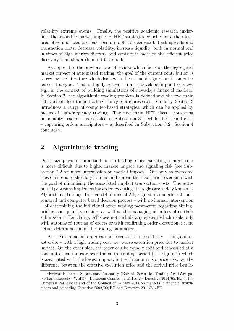
At one extreme, an order can be executed at once entirely – using a mar-ket order – with a high trading cost, i.e. worse execution price due to marketimpact. On the other side, the order can be equally split and scheduled at aconstant execution rate over the entire trading period (see Figure 1) whichis associated with the lowest impact, but with an intrinsic price risk, i.e. thedifference between the effective execution price and the arrival price bench-
2Federal Financial Supervisory Authority (BaFin), Securities Trading Act (Wertpa-pierhandelsgesetz - WpHG); European Comission, MiFid 2 – Directive 2014/65/EU of theEuropean Parliament and of the Council of 15 May 2014 on markets in financial instru-ments and amending Directive 2002/92/EC and Directive 2011/61/EU
3
mark due to random price movements (shortfall). The optimal schedulinglies in-between this range bounded by the minimum variance strategy, at oneside, and the minimum impact strategy, at the other side. As expressed inKissell and Malamut (2005), a trader faces the trade-off/dilemma of tradingtoo quickly (aggressively) and trading too slowly (passively).
t
v(t)
,x(t
)
020
4060
80
0 −10 −10 −10 −10 −10 −10 −10 −10 −10 −10
100
90
80
70
60
50
40
30
20
10
0
Figure 1: A linear execution schedule – time weighted average price (TWAP)
The line plot represents the trajectory x(t), i.e. the remaining order size to be executed attime t. The bar chart illustrates the trading rate ν(t), the slice of the entire order executedat time t.
A formalization of the order scheduling problem is provided in Almgrenand Chriss (2001). The objective is to compute a trajectory function x(t)representing the number of units remaining to be traded at time t, with theinitial target x(0) = X0 and the completely executed order at the end of theexecution time x(T ) = 0. The corresponding trading rate, i.e. the numberof units to be traded in one time interval, is denoted ν(t) = x(t − 1) − x(t)(see an example of a constant trading rate in Figure 1). The optimizationproblem consists in finding the optimal balance between the expected tradingcosts and the uncertainty of these costs due to the exposure to timing risk:
minx
(E[C(x)] + λ Var[C(x)]) , (2.1)
where:- C(x) cost of deviating from the benchmark- Var[C(x)] variance of the execution cost as a proxy for risk- λ ≥ 0 agent’s level of risk aversion which penalizes the variance relative tothe expected cost
Johnson (2010) provides a classification of AT based on its target objec-tives into impact-driven, cost-centric and opportunistic algorithms. The firstcategory is schedule-based and seeks to minimize the overall market impact
4
costs by splitting larger orders over time. E.g., the Time Weighted AveragePrice (TWAP) strategy – also illustrated in Figure 1 – slices the originalorder into equal parts which are spread over fixed and equal time intervalsthroughout the day. Another impact-driven strategy, Volume Weighted Av-erage Price (VWAP), tracks statically created trajectories based on historicalvolume profiles (see Subsection 2.1 for more details). Dynamic tracking algo-rithms such as Percentage of Volume (POV) – also known as Volume Inline– try to participate in the market at a given rate in proportion with themarket’s actual volume. Cost-centric algorithms try to reduce transactioncosts by balancing implicit costs, such as market impact, and the exposureto timing risk by taking into account the investor’s level of urgency or riskaversion. E.g., Implementation Shortfall (IS) – also known as Arrival Price– determines the optimal trade horizon, as well as the appropriate trad-ing schedule, by applying various cost and market models which take intoaccount factors such as order size, available time, expected price change (al-pha), expected liquidity and volatility (see Subsection 2.2 for more details).Finally, opportunistic algorithms, such as Price Inline (PI), are variants ofthe impact-driven algorithms which are sensitive and self-adjusting to thecurrent market conditions.
Fabozzi, Focardi, Kolm et al. (2010) identify IS and VWAP as the twomost popular execution strategies. While VWAP’s execution costs are as-sessed relative to the benchmark with the same name (see Subsection 2.1)and the algorithm aims at reducing the absolute market impact costs, IS isbenchmarked to the arrival price – the price prevailing at the beginning of theexecution period – and is optimized towards minimizing the overall potentialrisk-adjusted costs, with respect to a predefined coefficient of risk aversion.In the following two subsections, selected variants of these two algorithmictrading strategies are presented.
2.1 Volume Weighted Average Price
Volume-Weighted Average Price is an automated participation strategy whichtries to achieve an execution price close to the VWAP benchmark. The lattercorresponds to the overall turnover divided by the total volume VWAP =∑n
vn pn/∑n
vn.3 According to Madhavan (2002), the main reason for choos-
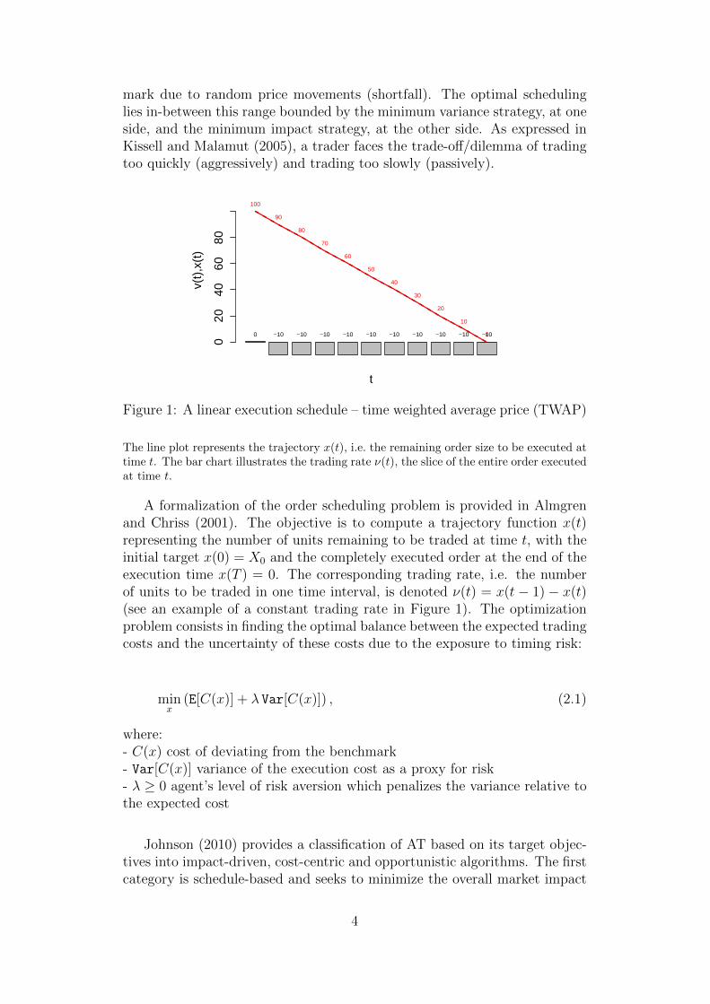
ing this strategy is due to the benchmark choice, i.e. the criteria used formeasuring the execution performance. Thus, VWAP is an ideal option forpassive traders with no alpha and no need for urgency. The actual imple-mentation consists in splitting the initial order over the entire trading period– usually the entire or a large part of a trading day – based on a model ofthe historical fractional daily volume pattern (see Figure 2). Since the actualintraday volume pattern for any single day will be different from the histor-ical average, the VWAP is not guaranteed and will mostly randomly miss
3If a large order represents too much (> 30%) of the average daily volume, VWAP haspractically no meaning.
5
the actual VWAP, especially on days with highly unusual volume patterns.However, with the help of automation, the order can be split in a very largenumber of smaller orders which can be spread over finer time grids and thusreduce to some extent the problems associated with the model’s noise.
t
v(t)
0e+
002e
+05
4e+
05
9 11 13 15 17
t
v(t)
,x(t
)
020
4060
800 −13 −10 −11 −7 −11 −8 −11 −13 −16
100
87
77
66
59
48
40
29
16
0
Figure 2: VWAP
The left plot presents the hourly average values of the trading volume for Siemens (SIE),traded at Xetra Frankfurt during the entire February 2012 – the notorious U-shape orthe volume “smile” can be roughly observed. The right plot describes the evolution ofthe trading schedule and the hourly order sizes, corresponding to the historical volumepattern, i.e. the nine one hour bins in the left plot.
The VWAP can be improved by replacing the standard historical pat-tern with other models of the intraday volume dynamics. E.g., Bia lkowski,Darolles and Le Fol (2008) suggest a dynamical volume model, which de-composes the traded volume in two parts: one reflecting the common andseasonal market evolution – modeled by an extension of CAPM with factorsestimated by principal component analysis – and a second one capturing theintraday specific volume dynamics by means of an ARMA(1,1) or a SETARmodel. As a difference form the statical VWAP, the trading schedule cannotbe determined in advance at the start of the trading period, but needs to beupdated step-by-step, based on the one-step ahead prediction of the dynamiccomponent which takes into consideration also the previous intraday periodrealization.
2.2 Implementation Shortfall
As its name suggests, Implementation Shortfall4 is benchmarked to the ar-rival price – the price prevailing at the beginning of the execution period –and is optimized towards minimizing the overall potential risk-adjusted costswith respect to a predefined coefficient of risk aversion. According to Fabozziet al. (2010), this strategy is especially appropriate for market participants
4The shortfall is the difference between the arrival and the effective execution price.
6
who know their risk-aversion profile and who have a strong belief about thefuture returns.
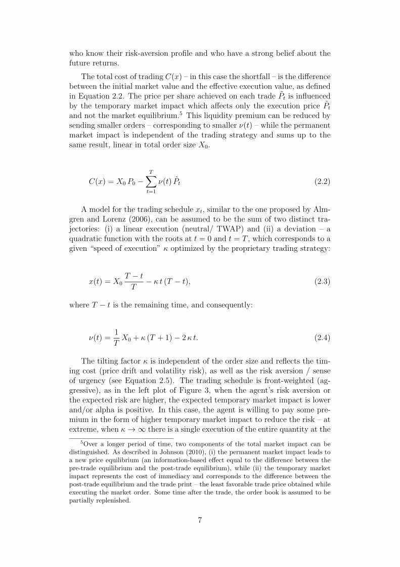
The total cost of trading C(x) – in this case the shortfall – is the differencebetween the initial market value and the effective execution value, as definedin Equation 2.2. The price per share achieved on each trade Pt is influencedby the temporary market impact which affects only the execution price Ptand not the market equilibrium.5 This liquidity premium can be reduced bysending smaller orders – corresponding to smaller ν(t) – while the permanentmarket impact is independent of the trading strategy and sums up to thesame result, linear in total order size X0.
C(x) = X0 P0 −T∑t=1
ν(t) Pt (2.2)
A model for the trading schedule xt, similar to the one proposed by Alm-gren and Lorenz (2006), can be assumed to be the sum of two distinct tra-jectories: (i) a linear execution (neutral/ TWAP) and (ii) a deviation – aquadratic function with the roots at t = 0 and t = T , which corresponds to agiven “speed of execution” κ optimized by the proprietary trading strategy:
x(t) = X0T − tT− κ t (T − t), (2.3)
where T − t is the remaining time, and consequently:
ν(t) =1
TX0 + κ (T + 1)− 2κ t. (2.4)
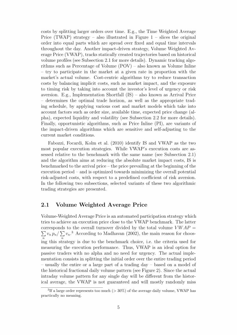
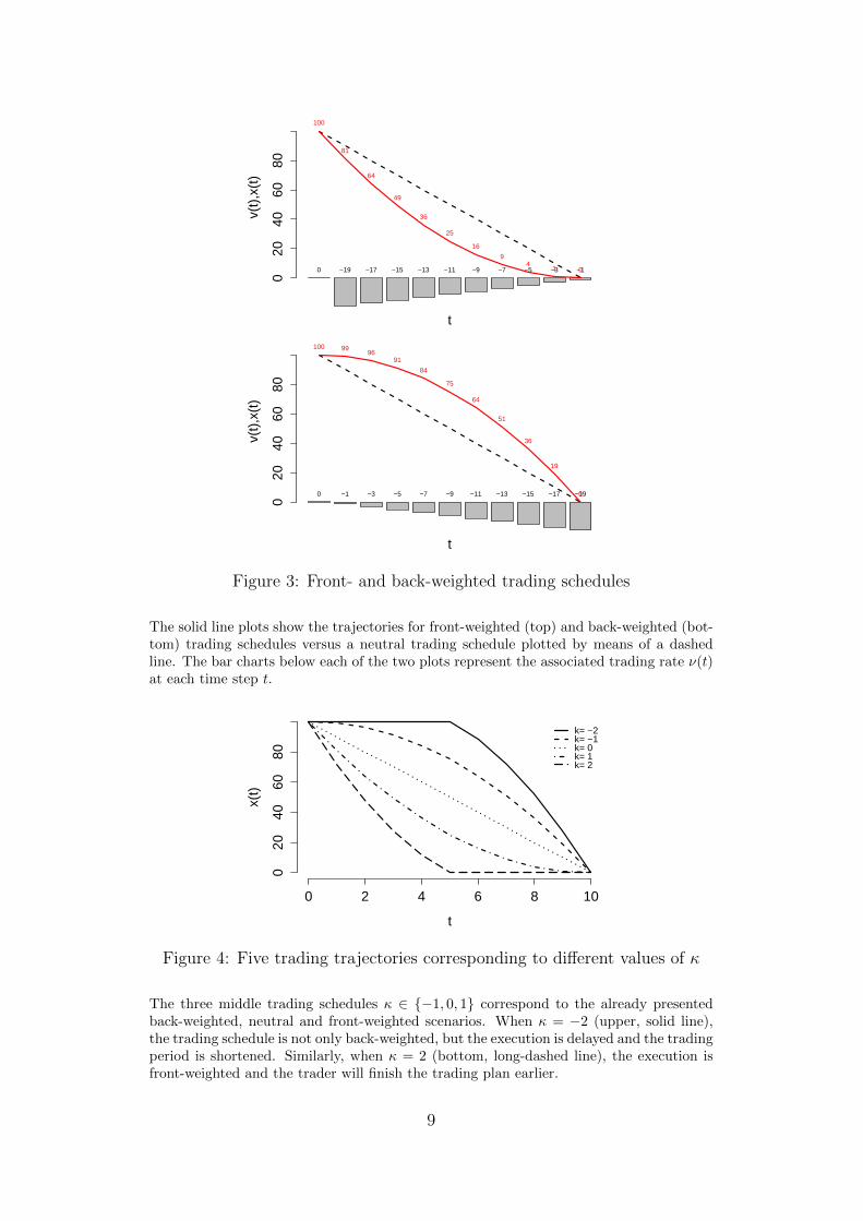
The tilting factor κ is independent of the order size and reflects the tim-ing cost (price drift and volatility risk), as well as the risk aversion / senseof urgency (see Equation 2.5). The trading schedule is front-weighted (ag-gressive), as in the left plot of Figure 3, when the agent’s risk aversion orthe expected risk are higher, the expected temporary market impact is lowerand/or alpha is positive. In this case, the agent is willing to pay some pre-mium in the form of higher temporary market impact to reduce the risk – atextreme, when κ→∞ there is a single execution of the entire quantity at the
5Over a longer period of time, two components of the total market impact can bedistinguished. As described in Johnson (2010), (i) the permanent market impact leads toa new price equilibrium (an information-based effect equal to the difference between thepre-trade equilibrium and the post-trade equilibrium), while (ii) the temporary marketimpact represents the cost of immediacy and corresponds to the difference between thepost-trade equilibrium and the trade print – the least favorable trade price obtained whileexecuting the market order. Some time after the trade, the order book is assumed to bepartially replenished.
7
start of the trading period. Conversely, when alpha is negative or when theagent is risk loving (negative λ), the trading schedule becomes back-weighted(passive), as in the right plot of Figure 3. Finally, when κ = 0, i.e. no signif-icant drift is expected (zero or small alpha) and/or the expected temporarymarket impact is higher, the execution is neutral – constant trading rate.6
κ =λασ
η, (2.5)
where:- α price change expectation7
- σ expected stock volatility- η expected temporary market impact cost8
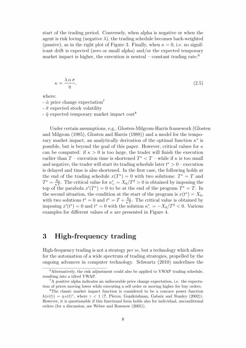
Under certain assumptions, e.g., Glosten-Milgrom-Harris framework (Glostenand Milgrom (1985), Glosten and Harris (1988)) and a model for the tempo-rary market impact, an analytically derivation of the optimal function κ∗ ispossible, but is beyond the goal of this paper. However, critical values for κcan be computed: if κ > 0 is too large, the trader will finish the executionearlier than T – execution time is shortened T ∗ < T – while if κ is too smalland negative, the trader will start its trading schedule later t∗ > 0 – executionis delayed and time is also shortened. In the first case, the following holds atthe end of the trading schedule x(T ∗) = 0 with two solutions: T ∗ = T andT ∗ = X0
κT. The critical value for κ∗+ = X0/T
2 > 0 is obtained by imposing thetop of the parabola x′(T ∗) = 0 to be at the end of the program T ∗ = T . Inthe second situation, the condition at the start of the program is x(t∗) = X0,with two solutions t∗ = 0 and t∗ = T + X0
κT. The critical value is obtained by
imposing x′(t∗) = 0 and t∗ = 0 with the solution κ∗− = −X0/T2 < 0. Various
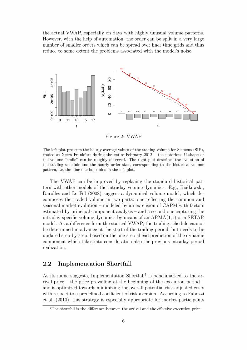
examples for different values of κ are presented in Figure 4.
3 High-frequency trading
High-frequency trading is not a strategy per se, but a technology which allowsfor the automation of a wide spectrum of trading strategies, propelled by theongoing advances in computer technology. Schwartz (2010) underlines the
6Alternatively, the risk adjustment could also be applied to VWAP trading schedule,resulting into a tilted VWAP.
7A positive alpha indicates an unfavorable price change expectation, i.e. the expecta-tion of prices moving lower while executing a sell order or moving higher for buy orders.
8The classic market impact function is considered to be a concave power functionh(ν(t)) = η ν(t)γ , where γ < 1 (?, Plerou, Gopikrishnan, Gabaix and Stanley (2002)).However, it is questionable if this functional form holds also for individual, unconditionalorders (for a discussion, see Weber and Rosenow (2005)).
8
t
v(t)
,x(t
)
020
4060
800 −19 −17 −15 −13 −11 −9 −7 −5 −3 −1
100
81
64
49
36
25
16
94
1 0
t
v(t)
,x(t
)
020
4060
80
0 −1 −3 −5 −7 −9 −11 −13 −15 −17 −19
100 9996
91
84
75
64
51
36
19
0
Figure 3: Front- and back-weighted trading schedules
The solid line plots show the trajectories for front-weighted (top) and back-weighted (bot-tom) trading schedules versus a neutral trading schedule plotted by means of a dashedline. The bar charts below each of the two plots represent the associated trading rate ν(t)at each time step t.
0 2 4 6 8 10
020
4060
80
t
x(t)
k= −2k= −1k= 0k= 1k= 2
Figure 4: Five trading trajectories corresponding to different values of κ
The three middle trading schedules κ ∈ {−1, 0, 1} correspond to the already presentedback-weighted, neutral and front-weighted scenarios. When κ = −2 (upper, solid line),the trading schedule is not only back-weighted, but the execution is delayed and the tradingperiod is shortened. Similarly, when κ = 2 (bottom, long-dashed line), the execution isfront-weighted and the trader will finish the trading plan earlier.
9
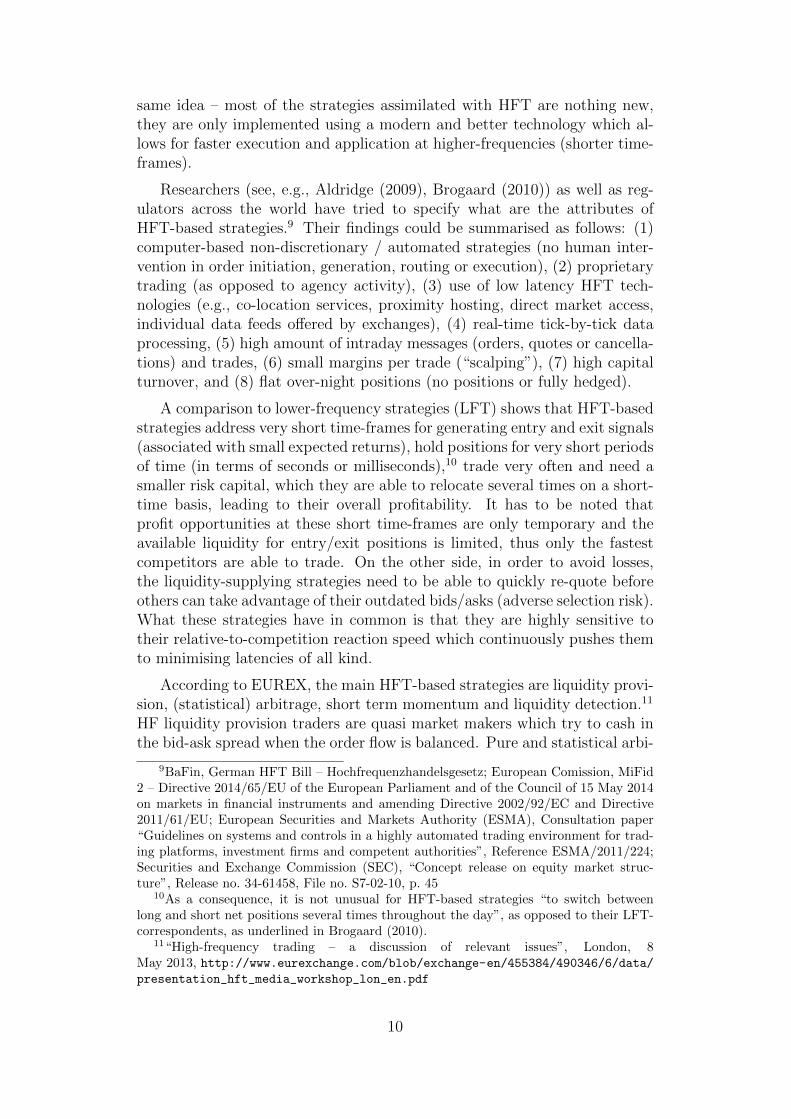
same idea – most of the strategies assimilated with HFT are nothing new,they are only implemented using a modern and better technology which al-lows for faster execution and application at higher-frequencies (shorter time-frames).
Researchers (see, e.g., Aldridge (2009), Brogaard (2010)) as well as reg-ulators across the world have tried to specify what are the attributes ofHFT-based strategies.9 Their findings could be summarised as follows: (1)computer-based non-discretionary / automated strategies (no human inter-vention in order initiation, generation, routing or execution), (2) proprietarytrading (as opposed to agency activity), (3) use of low latency HFT tech-nologies (e.g., co-location services, proximity hosting, direct market access,individual data feeds offered by exchanges), (4) real-time tick-by-tick dataprocessing, (5) high amount of intraday messages (orders, quotes or cancella-tions) and trades, (6) small margins per trade (“scalping”), (7) high capitalturnover, and (8) flat over-night positions (no positions or fully hedged).
A comparison to lower-frequency strategies (LFT) shows that HFT-basedstrategies address very short time-frames for generating entry and exit signals(associated with small expected returns), hold positions for very short periodsof time (in terms of seconds or milliseconds),10 trade very often and need asmaller risk capital, which they are able to relocate several times on a short-time basis, leading to their overall profitability. It has to be noted thatprofit opportunities at these short time-frames are only temporary and theavailable liquidity for entry/exit positions is limited, thus only the fastestcompetitors are able to trade. On the other side, in order to avoid losses,the liquidity-supplying strategies need to be able to quickly re-quote beforeothers can take advantage of their outdated bids/asks (adverse selection risk).What these strategies have in common is that they are highly sensitive totheir relative-to-competition reaction speed which continuously pushes themto minimising latencies of all kind.
According to EUREX, the main HFT-based strategies are liquidity provi-sion, (statistical) arbitrage, short term momentum and liquidity detection.11
HF liquidity provision traders are quasi market makers which try to cash inthe bid-ask spread when the order flow is balanced. Pure and statistical arbi-
9BaFin, German HFT Bill – Hochfrequenzhandelsgesetz; European Comission, MiFid2 – Directive 2014/65/EU of the European Parliament and of the Council of 15 May 2014on markets in financial instruments and amending Directive 2002/92/EC and Directive2011/61/EU; European Securities and Markets Authority (ESMA), Consultation paper“Guidelines on systems and controls in a highly automated trading environment for trad-ing platforms, investment firms and competent authorities”, Reference ESMA/2011/224;Securities and Exchange Commission (SEC), “Concept release on equity market struc-ture”, Release no. 34-61458, File no. S7-02-10, p. 45
10As a consequence, it is not unusual for HFT-based strategies “to switch betweenlong and short net positions several times throughout the day”, as opposed to their LFT-correspondents, as underlined in Brogaard (2010).
11“High-frequency trading – a discussion of relevant issues”, London, 8May 2013, http://www.eurexchange.com/blob/exchange-en/455384/490346/6/data/presentation_hft_media_workshop_lon_en.pdf
10
trageurs compare prices of the same assets across different markets or acrosseconomically similar (correlated) products and take advantage of any marketinefficiencies. Short term momentum and liquidity detection strategies tryto anticipate the short-term market direction due to new information or justdue to participants’ order flow.
3.1 Passive HFT - liquidity traders
Traditionally, on-exchange designated market makers (DMM) or specialistshave played the role of providing liquidity by continuously double quotingbid and ask prices at which they are committed to buy and sell specific assetquantities. Trading is thus facilitated as other market participants are pro-vided with immediacy, i.e. the ability to trade quickly and with reduced trans-action costs. On the other side, when completing a round-trip, i.e. the buyand sell of the same quantity, without any price change, the market maker iscompensated with the bid-ask spread differential. In case of an unfavourableprice shift, the realised profit becomes smaller than the quoted spread or caneven turn into a loss. Besides exchanges that employ a monopolistic mar-ket maker (e.g., NYSE), other exchanges (e.g., NASDAQ) rely on a differentstrategy for liquidity provision by allowing for multiple market-makers, wherethe overall performance comes from competition, rather than from strict indi-vidual obligations. In the case of exchanges which implement a maker-takerpricing model (e.g., NYSE Euronext’s Arca Options platform, NASDAQ’sNOM platform, BATS Global Markets options exchange), market-makershave an extra revenue source consisting in the rebates paid by the exchangefor passively providing limit orders, which are matched by liquidity-takingmarket orders – as opposed to standard equal pricing.
According to Harris (2002), vanilla market making strategies – which donot also speculate, hedge, or invest – are uninformed with respect to thefair value of the underlying assets and do not form expectations about thefuture market direction. Therefore, in order to avoid any inventory risk,market makers try to keep their inventory under control by quoting priceswhich produce two-sided order flows. When their inventory deviates fromthe target levels, market makers have to adjust their quotes (bid/ask prices,spread width, bid/ask quantities) in order to stimulate order flow which willoffset their imbalance. According to Aldridge (2009), another risk of marketmaking, which is compensated by the bid-ask spread, is the time-horizonrisk – the risk of an adverse market move decreases proportionally with theremaining trading time.12
Eventually, the specific levels of inventory targets, maximum allowed im-balances and holding time before restoring target inventories depend to agreat extent on the degree of information about the market equilibrium price– the larger the confidence in the estimated future price dynamics, the lower
12In other words, the spreads at the beginning of the trading session are larger thannear its end.
11
the perceived adverse selection risk and the higher the willingness to takelarge positions and hold them for a longer period of time in order to increaserealised spreads and profitability, accordingly.
Passive HFTs apply similar market making strategies, which are alsoknown as electronic liquidity provision (ELP), seeking to capture both thebid-ask spread and the rebates paid by the trading venues as incentives forposting liquidity. They are very poorly informed about fundamental valuesand therefore try to minimize the risk of liquidity provision by quickly off-setting even small inventory imbalances or by trying to identify toxic orderflow, which ultimately leads to opening positions against the future marketmove (for more details on toxic order flow, see Easley, de Prado and O’Hara(2012)). Their round-trip gains and inventory sizes are smaller than the onesof better informed market makers, but their overall profitability comes froma larger number of round-trips due to quoting more often at the best bid andbest ask, leading to a higher cumulative spread. HFT market makers com-pete to be the first counterparts in providing liquidity, as well as to profitablyclose their positions, which makes it vital being able to quickly update theiroutstanding orders in face of a changing market state.
The strategies employed by passive HFTs are sometimes referred to asquasi market making, because HFTs can suspend their activity whenever themarket state would lead to their unprofitability, e.g., due to high volatility ortrending, as they face no legal obligation to maintain quotes and guaranteemarket liquidity. Therefore, there is a general critique that the liquidity pro-vided by HFT is often illusory, since HFTs stay in the market only when theyare confident to make profits and retreat or even turn into liquidity-consumersunder adverse conditions. In Government Office For Science (2012), thisphenomena is named periodic illiquidity and is also explained by the oppor-tunistic style and tight risk management of HFT market makers. Moreover,a particular type of ELP, known as rebate arbitrage, tries to profit only fromcollecting liquidity rebates paid by the trade venue by opening and clos-ing positions at the same price on different exchanges (no spread capture),without really contributing to liquidity. Menkveld (2011) states that HFT“cream skimming” strategies, requiring little capital, have driven out tradi-tional market makers with large capital and inventories, leading to a drasticchange in the structure of liquidity provision sources, with large potentialimplications for the market dynamics in times of stress. On the other side,the Eurex Exchange finds evidence against this critique, by analyzing the be-havior of HFTs on the 25th of August, 2011 – a high volatile day for the DAXFutures (FDAX).13 The report concludes that HFTs actually contribute toliquidity and prevent fast price movements during periods of high volatilityor strong directional trading.
Nevertheless, some ELP strategies are considered to be used as signal de-tectors of large institutional block orders, which launch active HFT strategies
13“High-frequency trading in volatile markets – an examination”, Eurex Exchange,November 2011.
12
seeking to profit on this new information, and ultimately lead to amplifyinginvestors’ market impact (more details in Subsection 3.2).14
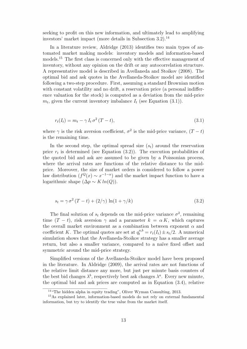
In a literature review, Aldridge (2013) identifies two main types of au-tomated market making models: inventory models and information-basedmodels.15 The first class is concerned only with the effective management ofinventory, without any opinion on the drift or any autocorrelation structure.A representative model is described in Avellaneda and Stoikov (2008). Theoptimal bid and ask quotes in the Avellaneda-Stoikov model are identifiedfollowing a two-step procedure. First, assuming a standard Brownian motionwith constant volatility and no drift, a reservation price (a personal indiffer-ence valuation for the stock) is computed as a deviation from the mid-pricemt, given the current inventory imbalance It (see Equation (3.1)).
rt(It) = mt − γ It σ2 (T − t), (3.1)
where γ is the risk aversion coefficient, σ2 is the mid-price variance, (T − t)is the remaining time.
In the second step, the optimal spread size (st) around the reservationprice rt is determined (see Equation (3.2)). The execution probabilities ofthe quoted bid and ask are assumed to be given by a Poissonian process,where the arrival rates are functions of the relative distance to the mid-price. Moreover, the size of market orders is considered to follow a powerlaw distribution (fQ(x) ∼ x−1−α) and the market impact function to have alogarithmic shape (∆p ∼ K ln(Q)).
st = γ σ2 (T − t) + (2/γ) ln(1 + γ/k) (3.2)
The final solution of st depends on the mid-price variance σ2, remainingtime (T − t), risk aversion γ and a parameter k = αK, which capturesthe overall market environment as a combination between exponent α andcoefficient K. The optimal quotes are set at qa,bt = rt(It)±st/2. A numericalsimulation shows that the Avellaneda-Stoikov strategy has a smaller averagereturn, but also a smaller variance, compared to a naıve fixed offset andsymmetric around the mid-price strategy.
Simplified versions of the Avellaneda-Stoikov model have been proposedin the literature. In Aldridge (2009), the arrival rates are not functions ofthe relative limit distance any more, but just per minute basis counters ofthe best bid changes λb, respectively best ask changes λa. Every new minute,the optimal bid and ask prices are computed as in Equation (3.4), relative
14“The hidden alpha in equity trading”, Oliver Wyman Consulting, 2013.15As explained later, information-based models do not rely on external fundamental
information, but try to identify the true value from the market itself.
13
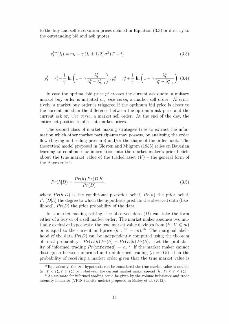
to the buy and sell reservation prices defined in Equation (3.3) or directly tothe outstanding bid and ask quotes.
rb,at (It) = mt − γ (It ± 1/2)σ2 (T − t) (3.3)
pbt = rbt−1
γln
(1− γ λbt
λbt − λbt−1
); pat = rat +
1
γln
(1− γ λat
λat − λat−1
)(3.4)
In case the optimal bid price pb crosses the current ask quote, a unitarymarket buy order is initiated or, vice versa, a market sell order. Alterna-tively, a market buy order is triggered if the optimum bid price is closer tothe current bid than the difference between the optimum ask price and thecurrent ask or, vice versa, a market sell order. At the end of the day, theentire net position is offset at market prices.
The second class of market making strategies tries to extract the infor-mation which other market participants may possess, by analysing the orderflow (buying and selling pressure) and/or the shape of the order book. Thetheoretical model proposed in Glosten and Milgrom (1985) relies on Bayesianlearning to combine new information into the market maker’s prior beliefsabout the true market value of the traded asset (V ) – the general form ofthe Bayes rule is:
Pr(h|D) =Pr(h)Pr(D|h)
Pr(D), (3.5)
where Pr(h|D) is the conditional posterior belief, Pr(h) the prior belief,Pr(D|h) the degree to which the hypothesis predicts the observed data (like-lihood), Pr(D) the prior probability of the data.
In a market making setting, the observed data (D) can take the formeither of a buy or of a sell market order. The market maker assumes two mu-tually exclusive hypothesis: the true market value deviates from (h : V ≶ m)or is equal to the current mid-price (h : V = m).16 The marginal likeli-hood of the data Pr(D) can be independently computed using the theoremof total probability: Pr(D|h)Pr(h) + Pr(D|h)Pr(h). Let the probabil-ity of informed trading Pr(informed) = α.17 If the market maker cannotdistinguish between informed and uninformed trading (α = 0.5), then theprobability of receiving a market order given that the true market value is
16Equivalently, the two hypothesis can be considered the true market value is outside(h : V < Pb, V > Pa) or in-between the current market maker spread (h : Pb ≤ V ≤ Pa).
17An estimate for informed trading could be given by the volume imbalance and tradeintensity indicator (VPIN toxicity metric) proposed in Easley et al. (2012).
14
lower/higher is given by Pr(D|h) = 0.75.18 Complementary, the probabil-ity of a market order under the assumption of an “equal” market value isPr(D|h) = 1−Pr(D|h) = 0.25. If the market maker is uninformed, then theunconditional probabilities of the two hypothesis are Pr(h) = Pr(h) = 0.5.Finally, the optimal bid and ask quotes, which include the adverse tradingrisk and assume zero profit (perfect competition), are computed as expecta-tions of the true market value given the two possible market events:
Pb = E[V |sell] ;Pa = E[V |buy] (3.6)
The Das model in Das (2005, 2008) extends the theoretical model ofGlosten and Milgrom by introducing a method to explicitly compute thesolutions to the quote-setting Equation (3.6), based on an online probabilisticestimate of the true underlying value of the asset. This density estimate takesthe form of a discrete distribution Pr(V = x), computationally representedas a vector with a range from µV −4σV to µV +4σV , where µV and σ2
V are themean and variance of the true value. The vector is initialized with a normalpdf N(µV , σV ) and is continuously updated by means of a nonparametricdensity estimation technique. There are three possible market events whichlead to updating the density estimate: receiving a buy, a sell or no marketorder. E.g., in the case of a buy order, standard Bayesian updating, asdescribed in Equation (3.7), is applied over the entire vector. The buy priorPr(buy) in the denominator is the same for all x and can be ignored duringthe update, before renormalizing.
Pr(V = x|buy) =Pr(V = x)Pr(buy|V = x)
Pr(buy), (3.7)
where Pr(V = x) is the prior density estimate.
According to Equation (3.6), the market maker’s optimal quotes are equalto the conditional expected value given that a particular type of order isreceived. E.g., an approximation of the ask price Pa = E[V |buy] can becomputed as in Equation (3.8).
Pa =Vmax∑
xi=Vmin
xi Pr(V = xi|buy) =
Vmax∑xi=Vmin
xi Pr(V = xi)Pr(buy|V = xi)
Pr(buy)
(3.8)
18The market order can be generated either by an informed or uninformed trader. Ifthe trader were informed, the probability of placing exactly an order of the respective signis 100%, while if uninformed, the probability of placing a buy or sell order is equal to 50%.Therefore, the conditional probability Pr(D|h) = α+ 0.5 (1− α).
15
Such quotes correspond to a zero-profit situation and represent the max-imum bid price and the minimum ask price the market maker is willing toquote in order to cover the adverse selection risk.
Das (2005) also proposes a basic profit-making strategy, achieved bywidening the spread around the break-even bid-ask spread with a fixedamount. The market maker faces a trade-off between large spreads (higherprofits) with few round-trips and small spreads with many trades. The opti-mal solution of this trade-off depends on the market informativeness degree,as well as on the level of competition. When the competition between mar-ket makers is high, Das (2008) suggests placing bids and asks just inside thecurrent spread as long as they are associated with a non-negative expectedprofit, i.e. the Glosten and Milgrom condition. It is to be noted that the onlysignals about the true market value come from direct trading, so that quoteplacement plays an important role in sampling the distribution on tradesinduced by the true value.
The prior of a buy order is:
Pr(buy) =Vmax∑
xi=Vmin
Pr(V = xi)Pr(buy|V = xi) (3.9)
The computation of the above conditional probabilities depend on as-sumptions about the trader population. Das (2008) describes a market makertrading against informed agents, who only know the true value under the formof a noisy signal W = V + N(0, σW ).19 In other words, the noisy informedtrader sends a buy market order if W > Pa, a sell order if W < Pb and noorder if Pb ≤ W ≤ Pa.
20 Under these conditions, the conditional probabilityof a buy order is:
Pr(buy|V = x) = Pr(W > Pa) = Pr(N(0, σW ) > Pa − x) (3.10)
The optimum ask and bid quotes are the solutions of the fixed point equa-tions given by substituting Equation (3.10) into Equation (3.8). Das (2005)also finds out that, following a fundamental shock, the market-maker’s spreadincreases, reflecting its uncertainty about the underlying true value. Whilethe probability mass of the density estimate becomes more concentrated,spreads also get lower. The drawback is that the pdf values in the outer re-gions are also getting very small and hinder the estimate update when futurefundamental shocks occur. A solution proposed by Das (2005) is to recenterthe density estimate around the current expected value and reinitialize itwith a normal distribution after a fundamental jump has happened – such
19The σW parameter can control for the level of order flow toxicity (informativeness).20The case of a mixed populations of uninformed and (perfectly or noisy) informed
traders is analysed in Das (2005) and described in Appendix A, B.
16
a moment could be identified by an order imbalance-based classifier whichsimply counts the difference between the number of buy and sell orders (orbought and sold volumes) over a certain amount of time. Another extension,which takes into account also the portfolio risk, is presented in Das (2005).The proposed technique consists in shifting the pre-determined bid and askquotes with a linear function of the current inventory I: f(I) = −γ I, whereγ is a risk-aversion coefficient.21
Another market making model based on the Bayesian framework is in-troduced in Lin (2006). This time, the true value belief is updated by meansof a discrete Kalman filter, where the measurement is given by the net orderflow observed over some period of time. A different framework used to de-rive market making algorithms is reinforcement learning. Chan and Shelton(2001) train a market-maker strategy which observes three (discrete) statevariables: own inventory, order flow imbalance, bid-ask spread. The marketmaker’s set of actions include changing of the bid and/or ask prices, while thequoted sizes remain fixed. Finally, the reward function takes into considera-tion multiple objectives by means of a weighted-linear combination betweenprofit and bid-ask spread (as a measure of market quality).
3.2 Active HFT - order anticipators
As opposed to their passive counterpart, active HFTs act as liquidity takers,by trading with aggressive, liquidity-consuming market-orders. There aretwo main lines of active HFT development: the first one seeks to predictmarket momentum and incoming order-flow and makes profits from short-term market shifts, while the second one tries to exploit the technologicalstructure of the trading network system and superior speed advantage inorder to detect and “front run” distributed executions of large orders.
Many order anticipator strategies have existed before the advent of HFTand have only been adapted and applied at higher-frequencies, where humantraders are not able to react. Traditionally, according to Harris (2002), orderanticipators try to profit from information about third parties’ trading inten-tions, rather than from own fundamental information regarding the tradedasset. This type of profit-motivated speculators, also described as “parasitictraders” or “predatory”, can be further subdivided between front runners,sentiment-oriented technical traders and squeezers. While front-running andsqueezing are considered to be illegal strategies, due to exploiting confidentialinformation or being guilty of market manipulation, the sentiment-orientedtechnical traders (technical analysts or chartists) use public available infor-mation in order to predict future price returns. Depending on the underlyingtime-frame, various sources of information can be used by these technicalstrategies. For example, end-of-day strategies process aggregated informa-tion related to the daily price (open, high, low, close, average, median) or
21Alternatively, a sigmoid function allows for a gradual increase, as well as for limitingthe inventory control impact.
17
to the daily turnover in order to generate profitable trading signals. On theother side, intraday trading relies on additional information available at themarket microstructure level, such as order book liquidity, order flow, tradeand tick history. The main idea is to identify persistent relationships betweenvarious market indicators and future short-term market moves or incomingcustomer order flow, upon which profitable trading strategies can be built.
In a high-frequency setting, the analysed time-series are usually in a rawformat (tick-by-tick), i.e. without any aggregation, and the information pro-cessing as well as trading are conducted in a non-discretionary and automatedfashion by means of computer programs (no human intervention). The actualtrading rules can either be specified by a human specialist or can be “learned”from past data through various quantitative and computational methods(e.g., machine learning, artificial intelligence, evolutionary techniques). Arelated general concern, conformed by Brogaard (2010), is that HFT-basedstrategies are not very diversified or, equivalently, their trading signals arehighly correlated, leading to an exacerbation of market movements.
One simple HFT strategy proposed by Aldridge (2009) is based on orderflow short-term autocorrelation, which consists in opening position in thedirection of the order flow imbalance, i.e. the difference between the cumu-lative number/volume of buy and sell orders, or buyer- and seller-initiatedtrades. Another strategy relies on mimicking aggressive trading, as a proxyfor informed traders’ expectations. An indicator measuring the orders’ ag-gressiveness can be computed as the percentage of market as opposed to limitorders. Besides the share of market orders, where limit orders are placed,i.e. the shape of the order book, can also reveal the future expectations ofmarket participants. For example, the order book imbalance, quantified asthe difference between the cumulated volumes up to a certain depth levelon each side of the order book, can influence the aggressiveness of incomingorders in two ways.22 When their side of the book is thicker and crowded,traders price their orders more aggressively in order to increase their orderexecution probability (competition effect). Conversely, traders become lessaggressive when the opposite side is deeper, forecasting a favorable short-term order flow (strategic effect). Order-flow related are also the inter-tradeand price/volume durations, which can indicate changes in liquidity andvolatility due to new information.23 Short-term momentum/reversal can alsobe detected by means of econometric models taking into consideration phe-nomenological observations such as autocorrelation of price returns (serialdependence for small intraday scales), fat tails and volatility clustering.
A second class of active HFTs tries to identify patterns of execution al-gorithms (processing large institutional orders) and trade ahead the remain-
22Alternatively, the book imbalance and the short-term price return can be assessedby comparing the bid-ask midpoint with the weighted price at a given depth of the orderbook as in Cao, Hansch and Wang (2009).
23The time interval between subsequent volume changes of a specified magnitude isknown as volume duration.
18
ing execution program (“electronic front-running”). For example, when theliquidity is fragmented over a number of trading venues, the execution algo-rithms route their orders across different locations, and in case their tradingactivity is exposed, ultra-HFTs can exploit their ultra-low-latency compet-itive advantage and profit from the “working” of the large order (latency-based arbitrage). Similarly, algorithmic traders can be taken advantage of iftheir order generating pattern is predictable from the observable order flow(order-flow detection). In the same framework of multiple exchanges, ultra-HFTs can profit from temporary market inefficiencies by picking off outdatedorders belonging to market participants with a higher reaction latency (slow-market arbitrage). As a negative side effect, the institutional investor suffersfrom an increased market price impact and, consequently, a reduced “alpha”.Retail investors are usually not affected because their orders are too small.First of all, it is questionable whether the term “front-running” is justified ornot in this case, since the ultra-HFTs do not have direct access to the actualorder to be executed, and this is only induced in a noisy manner from publictrading data. On the execution side, smart routing strategies which are ableto minimize the speed advantage of ultra-HFTs have been developed. E.g.,Royal Bank of Canada’s THOR R© routing technology precomputes the rout-ing latencies and sends the different slices of the total order in such a wayso they reach the targeted trading venues at the same time and thereforeeliminating any information leakage.
4 Conclusions
The current contribution describes a range of computer-based trading strate-gies which are widely applied by market participants, in the context of nowa-days increased trading automation and market fragmentation. The strategieswere classified both based on the profile of market participants and on thetechnology type. Informed traders use algorithmic trading strategies in or-der to reduce their transaction costs and smart order routing technologiesin order to minimize information leakage. Based on their risk profile andon the performance benchmark for the execution, different algorithmic trad-ing strategies are preferred. The classic optimisation problem of trading hasbeen defined and both basic implementations, as well as extended versionsof the two main algorithmic trading strategies, i.e. Volume Weighted Aver-age Price and Implementation Shortfall, have been introduced. In the caseof uninformed liquidity traders or market-makers, high-frequency tradingtechnologies have been introduced in order to maintain the low-latency ad-vantage as trading edge. Several models of market making strategies, whichcan be classified in two types based on their core objective, i.e. inventory-and information-based models, have been introduced. For the latter type,two different machine learning frameworks, i.e. Bayesian learning and Re-inforcement learning, have been discussed. Finally, order anticipators makeuse of the increased computational power in order to process in real time
19
a larger amount of trading information – including the rich microstrucutredata, e.g., order flow and order book data – and to develop new predictivemodels which can be applied at high-frequency time-series. Others simplyrely on their ultra-low-latency advantage and speculate the fragmented struc-ture of the trading network in order to detect and “front run” the executionof large orders.
References
Aldridge, I. (2009). High-frequency trading: a practical guide to algorithmicstrategies and trading systems, Vol. 459, John Wiley & Sons, Hoboken,New Jersey.
Aldridge, I. (2013). High-frequency trading: a practical guide to algorith-mic strategies and trading systems, Second Edition, John Wiley & Sons,Hoboken, New Jersey.
Almgren, R. and Chriss, N. (2001). Optimal execution of portfolio transac-tions, Journal of Risk 3: 5–40.
Almgren, R. and Lorenz, J. (2006). Bayesian adaptive trading with a dailycycle, The Journal of Trading 1(4): 38–46.
Avellaneda, M. and Stoikov, S. (2008). High-frequency trading in a limitorder book, Quantitative Finance 8(3): 217–224.
Bia lkowski, J., Darolles, S. and Le Fol, G. (2008). Improving vwap strategies:a dynamic volume approach, Journal of Banking & Finance 32(9): 1709–1722.
Brogaard, J. (2010). High frequency trading and its impact on market quality,Northwestern University Kellogg School of Management Working Paper66.
Cao, C., Hansch, O. and Wang, X. (2009). The information content of anopen limit-order book, Journal of futures markets 29(1): 16–41.
Chan, N. T. and Shelton, C. (2001). An electronic market-maker, TechnicalReport 195, Massachusetts Institute of Technology – Artificial Intelli-gence Laboratory.
Das, S. (2005). A learning market-maker in the glosten–milgrom model,Quantitative Finance 5(2): 169–180.
Das, S. (2008). The effects of market-making on price dynamics, Proceed-ings of the 7th international joint conference on Autonomous agents andmultiagent systems-Volume 2, International Foundation for AutonomousAgents and Multiagent Systems, pp. 887–894.
20
Easley, D., de Prado, M. and O’Hara, M. (2012). Flow toxicity and liquidityin a high-frequency world, Review of Financial Studies 25(5): 1457–1493.
Fabozzi, F. J., Focardi, S. M., Kolm, P. N. et al. (2010). Quantitative equityinvesting: Techniques and strategies, John Wiley & Sons.
Glosten, L. R. and Harris, L. E. (1988). Estimating the components of thebid/ask spread, Journal of financial Economics 21(1): 123–142.
Glosten, L. R. and Milgrom, P. R. (1985). Bid, ask and transaction prices ina specialist market with heterogeneously informed traders, Journal offinancial economics 14(1): 71–100.
Government Office For Science (2012). Foresight: The future of computertrading in financial markets, Technical report.
Harris, L. (2002). Trading and exchanges: Market microstructure for practi-tioners, Oxford University Press, USA.
Johnson, B. (2010). Algorithmic Trading & DMA: An introduction to directaccess trading strategies, 4Myeloma Press, London.
Kissell, R. and Malamut, R. (2005). Understanding the profit and loss dis-tribution of trading algorithms, Trading 2005(1): 41–49.
Lillo, F., Farmer, J. and Mantegna, R. (2002). Single curve collapse of theprice impact function for the new york stock exchange, arXiv preprintcond-mat/0207428 .
Lillo, F., Farmer, J. and Mantegna, R. (2003). Master curve for price-impactfunction, Nature 421(129): 176–190.
Lin, H. (2006). Essays in market microstructure, PhD thesis, University ofWarwick.
Madhavan, A. N. (2002). Vwap strategies, Trading 2002(1): 32–39.
Menkveld, A. (2011). Electronic trading and market structure, UK Gov-ernment Office for Science, Foresight Driver Review - The Future ofComputer Trading in Financial Markets .
Plerou, V., Gopikrishnan, P., Gabaix, X. and Stanley, H. E. (2002). Quan-tifying stock-price response to demand fluctuations, Physical Review E66(2): 027104.
Schwartz, R. (2010). Dark pools, fragmented markets, and the quality ofprice discovery, The Journal of Trading 5(2): 17–22.
Vuorenmaa, T. (2012). The good, the bad, and the ugly of automated high-frequency trading, Technical report, Valo Research and Trading.
21

Weber, P. and Rosenow, B. (2005). Order book approach to price impact,Quantitative Finance 5(4): 357–364.
22
A Das model with uninformed and perfectly
informed traders
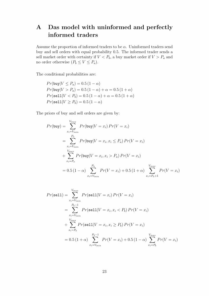
Assume the proportion of informed traders to be α. Uninformed traders sendbuy and sell orders with equal probability 0.5. The informed trader sends asell market order with certainty if V < Pb, a buy market order if V > Pa andno order otherwise (Pb ≤ V ≤ Pa).
The conditional probabilities are:
Pr(buy|V ≤ Pa) = 0.5 (1− α)
Pr(buy|V > Pa) = 0.5 (1− α) + α = 0.5 (1 + α)
Pr(sell|V < Pb) = 0.5 (1− α) + α = 0.5 (1 + α)
Pr(sell|V ≥ Pb) = 0.5 (1− α)
The priors of buy and sell orders are given by:
Pr(buy) =Vmax∑
xi=Vmin
Pr(buy|V = xi)Pr(V = xi)
=Pa∑
xi=Vmin
Pr(buy|V = xi, xi ≤ Pa)Pr(V = xi)
+Vmax∑xi=Pa
Pr(buy|V = xi, xi > Pa)Pr(V = xi)
= 0.5 (1− α)Pa∑
xi=Vmin
Pr(V = xi) + 0.5 (1 + α)Vmax∑
xi=Pa+1
Pr(V = xi)
Pr(sell) =Vmax∑
xi=Vmin
Pr(sell|V = xi)Pr(V = xi)
=
Pb−1∑xi=Vmin
Pr(sell|V = xi, xi < Pb)Pr(V = xi)
+Vmax∑xi=Pb
Pr(sell|V = xi, xi ≥ Pb)Pr(V = xi)
= 0.5 (1 + α)
Pb−1∑xi=Vmin
Pr(V = xi) + 0.5 (1− α)Vmax∑xi=Pb
Pr(V = xi)
23
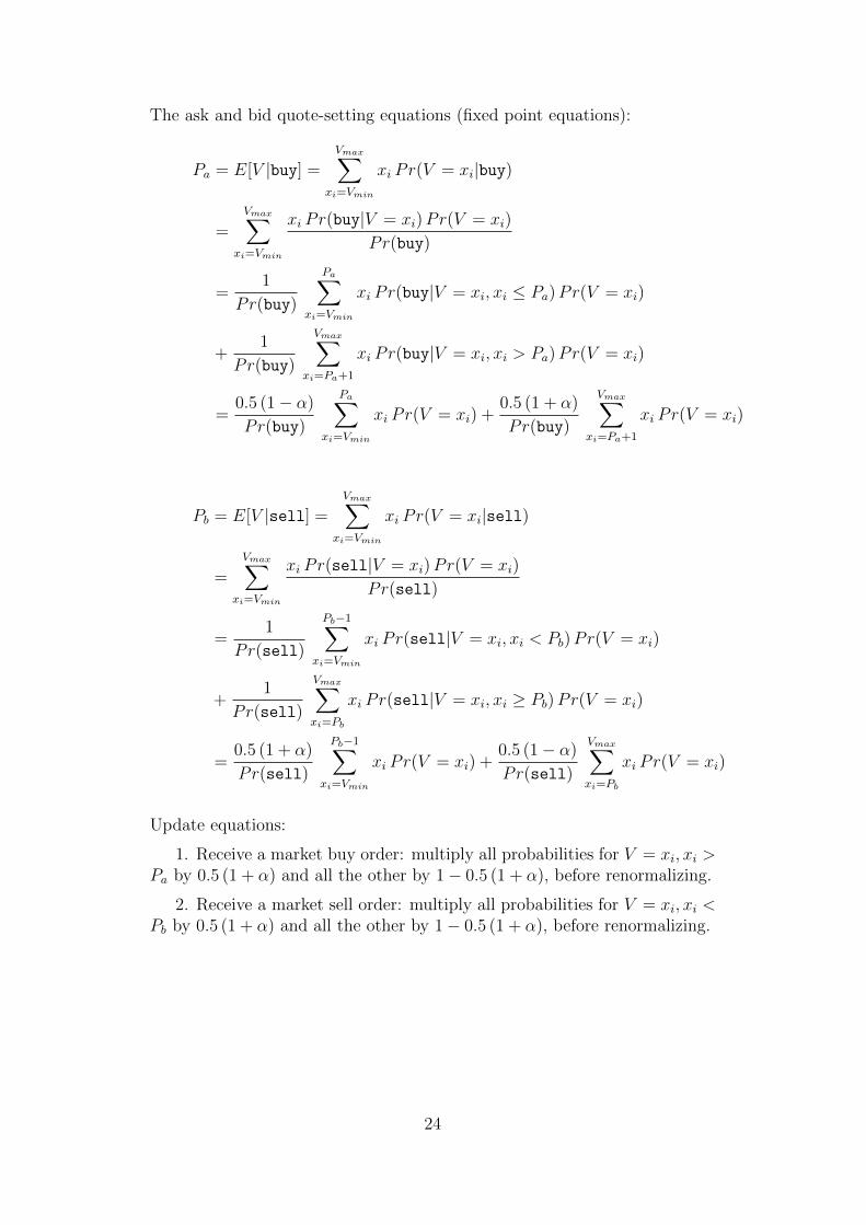
The ask and bid quote-setting equations (fixed point equations):
Pa = E[V |buy] =Vmax∑
xi=Vmin
xi Pr(V = xi|buy)
=Vmax∑
xi=Vmin
xi Pr(buy|V = xi)Pr(V = xi)
Pr(buy)
=1
Pr(buy)
Pa∑xi=Vmin
xi Pr(buy|V = xi, xi ≤ Pa)Pr(V = xi)
+1
Pr(buy)
Vmax∑xi=Pa+1
xi Pr(buy|V = xi, xi > Pa)Pr(V = xi)
=0.5 (1− α)
Pr(buy)
Pa∑xi=Vmin
xi Pr(V = xi) +0.5 (1 + α)
Pr(buy)
Vmax∑xi=Pa+1
xi Pr(V = xi)
Pb = E[V |sell] =Vmax∑
xi=Vmin
xi Pr(V = xi|sell)
=Vmax∑
xi=Vmin
xi Pr(sell|V = xi)Pr(V = xi)
Pr(sell)
=1
Pr(sell)
Pb−1∑xi=Vmin
xi Pr(sell|V = xi, xi < Pb)Pr(V = xi)
+1
Pr(sell)
Vmax∑xi=Pb
xi Pr(sell|V = xi, xi ≥ Pb)Pr(V = xi)
=0.5 (1 + α)
Pr(sell)
Pb−1∑xi=Vmin
xi Pr(V = xi) +0.5 (1− α)
Pr(sell)
Vmax∑xi=Pb
xi Pr(V = xi)
Update equations:
1. Receive a market buy order: multiply all probabilities for V = xi, xi >Pa by 0.5 (1 + α) and all the other by 1− 0.5 (1 + α), before renormalizing.
2. Receive a market sell order: multiply all probabilities for V = xi, xi <Pb by 0.5 (1 + α) and all the other by 1− 0.5 (1 + α), before renormalizing.
24
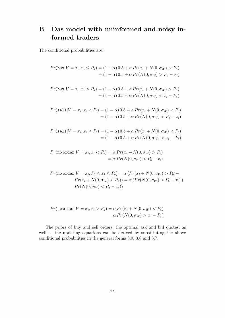
B Das model with uninformed and noisy in-
formed traders
The conditional probabilities are:
Pr(buy|V = xi, xi ≤ Pa) = (1− α) 0.5 + αPr(xi +N(0, σW ) > Pa)
= (1− α) 0.5 + αPr(N(0, σW ) > Pa − xi)
Pr(buy|V = xi, xi > Pa) = (1− α) 0.5 + αPr(xi +N(0, σW ) > Pa)
= (1− α) 0.5 + αPr(N(0, σW ) < xi − Pa)
Pr(sell|V = xi, xi < Pb) = (1− α) 0.5 + αPr(xi +N(0, σW ) < Pb)
= (1− α) 0.5 + αPr(N(0, σW ) < Pb − xi)
Pr(sell|V = xi, xi ≥ Pb) = (1− α) 0.5 + αPr(xi +N(0, σW ) < Pb)
= (1− α) 0.5 + αPr(N(0, σW ) > xi − Pb)
Pr(no order|V = xi, xi < Pb) = αPr(xi +N(0, σW ) > Pb)
= αPr(N(0, σW ) > Pb − xi)
Pr(no order|V = xi, Pb ≤ xi ≤ Pa) = α (Pr(xi +N(0, σW ) > Pb)+
Pr(xi +N(0, σW ) < Pa)) = α (Pr(N(0, σW ) > Pb − xi)+Pr(N(0, σW ) < Pa − xi))
Pr(no order|V = xi, xi > Pa) = αPr(xi +N(0, σW ) < Pa)
= αPr(N(0, σW ) > xi − Pa)
The priors of buy and sell orders, the optimal ask and bid quotes, aswell as the updating equations can be derived by substituting the aboveconditional probabilities in the general forms 3.9, 3.8 and 3.7.
25