Stabilization Policy: A Reconsideration

Janet L. Yellen and George A. Akerlof*

July 1, 2004 * Janet Yellen is President of the Federal Reserve Bank of San Francisco and Eugene E. and Catherine M. Trefethen Professor of Business and Professor of Economics at the University of California at Berkeley. George Akerlof is Koshland Professor of Economics at the University of California at Berkeley. This paper forms the basis for Janet Yellen’s Presidential Address to the Western Economic Association, delivered July 1, 2004 in Vancouver, British Columbia.

I. Introduction

In 1936 Keynes’s General Theory explained how fiscal and monetary policy could be

used to end depressions. Since that time no developed country has ever seen a downturn on the

scale of the 1930s. The General Theory was not just a how-to book on the avoidance of

depressions. It was an argument for stabilization policy itself.

The years since The General Theory have seen a revolt against Keynesian economics. In

a revisionist mode, Milton Friedman argued that countercyclical policy cannot affect the average

level of unemployment and output. Robert Lucas and Thomas Sargent (1979) went further,

contending that it is not only impossible to increase average output; it is also impossible to

stabilize it. More recently, Lucas (1987, 2003) has argued that policies to stabilize output, even

if effective, would yield negligible welfare gains. Thus, stabilization policy should not be a

macroeconomic priority.

Lucas’s conclusion notwithstanding, stabilization policy has long been an explicit or

implicit objective of monetary policy in most industrial countries, even including those countries

with inflation targets. The volatility of output has, in fact, declined in most major industrial

countries since the mid-1980s, and monetary policy arguably deserves at least partial credit.1

Mirroring practice, monetary policy research commonly takes it as “given” that, along with price

stability, stabilization policy—the minimization of squared deviations of output around

potential—is an appropriate policy objective.2 In this paper we explore the economic rationale

for stabilization as a policy goal, concluding that it does, in fact, deserve high policy priority.

We survey a large body of literature that critiques the validity of key assumptions in Lucas’s

argument. We also offer suggestive evidence that stabilization policy can significantly reduce

1 See Bernanke (2004). 2 See, for example, Clarida, Galí, and Gertler (1999).

2

average levels of unemployment by providing stimulus to demand in circumstances where

unemployment is high but underutilization of labor and capital does little to lower inflation. A

monetary policy that vigorously fights high unemployment should, however, also be

complemented by a policy that equally vigorously fights inflation when it rises above a modest

target level. The Federal Reserve Act thus wisely enunciated price stability and maximum

employment as twin goals for monetary policy.

II. The Case Against Stabilization Policy

Macroeconomic analysis typically assumes that social welfare depends negatively on

both inflation (above a modest target level, here assumed zero) and unemployment (above some

minimum, socially efficient level). For example, a standard social welfare function is the

discounted sum of period losses (Lt) of the form:3

(1) 2 2( (1 ) *)t t tL a u k u bπ= − − + ,

where tu and tπ are the unemployment and inflation rates in period t, and *u is the natural rate

of unemployment. The coefficient k is positive, reflecting the desirability of unemployment

below the natural rate. Because real economies deviate in many respects from perfect

competition, the natural rate of unemployment is likely to exceed the socially optimal

unemployment rate. For example, with monopolistic competition, goods are underproduced

because they are priced above marginal cost, so “potential output” is inefficiently low and

“equilibrium unemployment” is too high.

Standard macroeconomic analysis additionally assumes that inflation is determined by an

expectations-augmented, accelerationist Phillips curve of the form

3 See among others Barro and Gordon (1983, pp. 592-3).

3

(2) ( *)et t t tf u uπ π ε= − − + ,

where etπ is the expected inflation rate at time t (with expectations formed at 1−t ), and tε

captures supply shocks to the Phillips curve at t. Reflecting the inflationary effects of tighter

labor markets, 'f is positive; reflecting the definition of u*, the natural rate of unemployment,

as the rate of unemployment where actual and expected inflation match, (0)f is equal to zero.

In this formulation *u is the unique unemployment rate where inflation is stable. This Phillips

curve has the property that inflation rises (the price level accelerates) when u is below u*: since

actual inflation exceeds expected inflation, with adaptive expectations, inflation expectations rise

over time and are factored into wage and price setting. In contrast, when unemployment exceeds

the natural rate, actual inflation falls short of expected inflation, so inflation declines over time as

expectations adjust downward toward reality. With chronic high unemployment, deflation is

inevitable.

To reach the conclusion that the gains from stabilizing output are trivially small, Lucas

considers a representative agent with a stochastic consumption stream whose welfare is given by

the discounted sum of instantaneous utilities, which depend only on consumption and are

characterized by constant relative risk aversion. Thus, welfare is

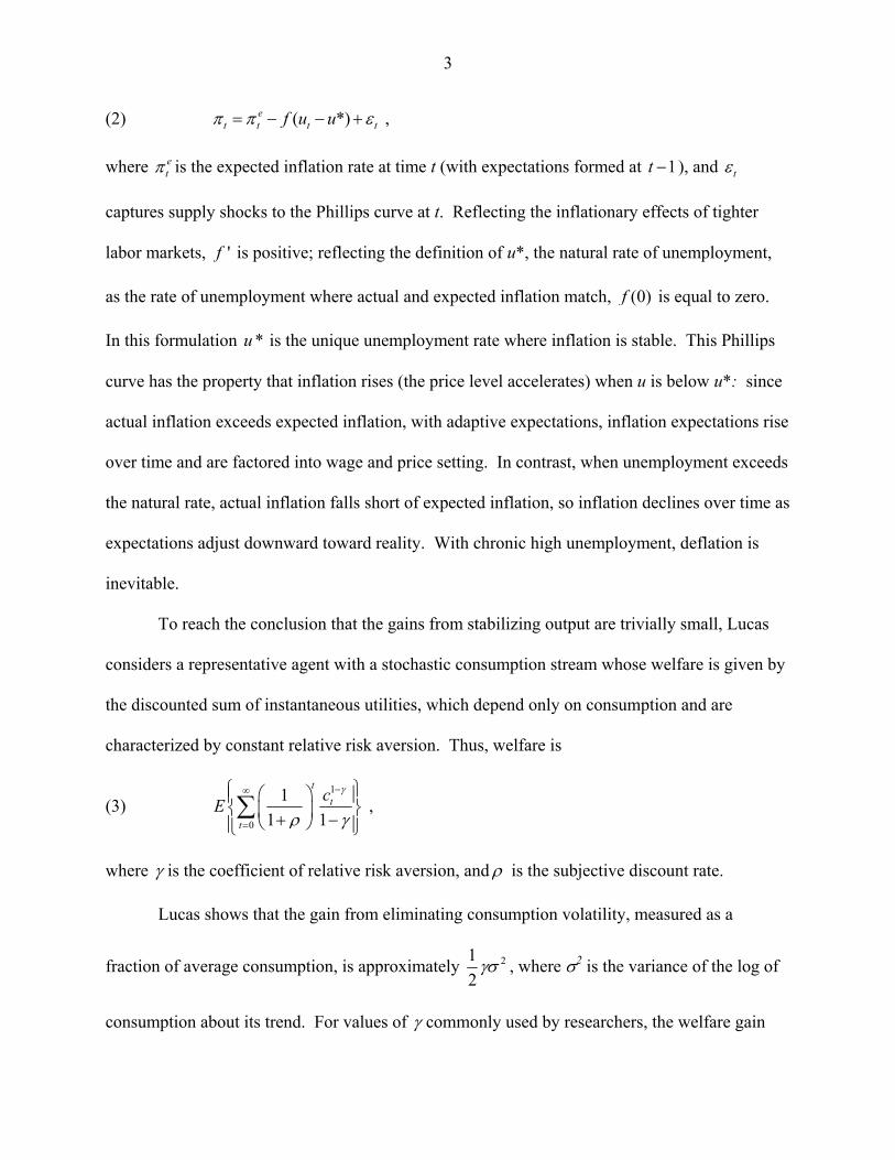
(3) 1

0

11 1

tt

t

cEγ

ρ γ

−∞

=

⎧ ⎫⎛ ⎞⎪ ⎪⎨ ⎬⎜ ⎟+ −⎝ ⎠⎪ ⎪⎩ ⎭∑ ,

where γ is the coefficient of relative risk aversion, and ρ is the subjective discount rate.

Lucas shows that the gain from eliminating consumption volatility, measured as a

fraction of average consumption, is approximately 212γσ , where σ2 is the variance of the log of

consumption about its trend. For values of γ commonly used by researchers, the welfare gain

4

from eliminating consumption volatility of the magnitude experienced in the United States

during the postwar period would be minuscule—on the order of one-twentieth of a percent of

average consumption.4 This result is not surprising. With differentiable utility it takes large

variations in most variables to have significant effects on welfare, and the percentage variation in

consumption over the business cycle is now small.5

Lucas’s calculation of very low returns from further stabilization of output results from

four separate assumptions regarding the nature of the macroeconomic loss function (1) and the

Phillips curve (2).6

First, Lucas’s assessment of the potential gains from stabilizing consumption ignores

possible relationships between the volatility of output and the volatility of inflation, captured in

the term 2tbπ in the standard loss function. Policies to stabilize unemployment (and

consumption) in the face of aggregate demand shocks simultaneously mitigate inflation volatility

according to (2), conferring welfare benefits beyond those assessed by Lucas.7 In contrast,

stabilizing unemployment (and consumption) in the face of supply shocks entails a policy

tradeoff between the volatility of inflation and unemployment (consumption). In this paper we

follow Lucas in ignoring the impacts of stabilization policy on inflation volatility.

4 See Lucas (2003), p. 4. Lucas notes that values of γ between 1 and 4 are commonly used in macroeconomics and public finance applications. Lucas’s baseline calculation assumes σ = 0.032 and γ =1, corresponding to log utility. 5 The losses also rise with the degree of risk aversion. 6 Romer (2001) provides an excellent discussion of the assumptions underlying Lucas’s findings and the implications of Lucas’s argument. In the tradition of modern macroeconomics textbooks, however, Romer fails to mention the possibility that the long-run Phillips curve may not always and everywhere be vertical, as emphasized in this paper. 7 Although it is commonly assumed, as in (1), that social welfare depends on both the mean and variance of inflation, the nature of the losses due to inflation volatility are not well understood. See Woodford (2002) for an interesting discussion.

5

Second, by considering paths of consumption that differ only in their volatility, Lucas

implicitly assumes that the Phillips curve is linear in unemployment. With a linear

accelerationist Phillips curve, average unemployment is identical along all unemployment paths

with the same initial and final inflation. Assuming further that unemployment is just an index

for consumption and varies linearly with it, stabilization policy can affect the volatility of

consumption, but not its mean, as Lucas assumes.

If the short-run Phillips curve (the f( ) function in (2)) is nonlinear, however, paths of

unemployment with the same beginning and ending inflation rate will differ somewhat in their

average unemployment rates. If f(u-u*) is concave, paths with lower unemployment volatility

will also enjoy lower average unemployment, higher average output, and higher average

consumption, contrary to Lucas’s assumption.

Lucas’s third assumption relates to the degree of nonlinearity of the function (1) relating

social welfare to unemployment. The loss due to consumption volatility is trivially small in part

because values of the rate of relative risk aversion Lucas considers plausible imply only very

modest curvature—thus, effective linearity—of the representative agent’s instantaneous utility

function.8 However, significant nonlinearity with respect to unemployment in the social welfare

function could reflect extreme losses in income for a small fraction of the population due to very

long spells of non-employment when unemployment is high, as well as substantially different

values of leisure for the marginally employed person in booms and troughs.9

8 Lucas notes that the losses due to consumption volatility are an order of magnitude higher using the far higher estimates of the degree of risk aversion needed to explain the equity premium puzzle. See, for example, Tallarini (2000), and Alvarez and Jermann (2000). However, as Lucas notes, not all volatility can be eliminated by stabilization policy, and not all risk aversion relates to business cycle fluctuations. 9 Lucas’s use of the representative agent framework assumes in addition that households are identical and individual risk is diversifiable.

6

Finally, Lucas’s calculation relies on the assumption that the Phillips curve is

accelerationist so that expected inflation impacts current inflation with a coefficient of unity.

Such an assumption is now considered standard and is surprisingly well-accepted: if all wage and

price setters are rational, the coefficient on expected inflation “should be” one. However,

assuming, even wishing, that wage setters and price setters are fully rational does not

automatically make it so. As we argue below, wage and price setters have their own ideas,

which led Irving Fisher (1928) to deplore their lack of rationality. If the coefficient on expected

inflation in wage or price equations is less than unity when inflation is low and unemployment is

high, policies to combat unemployment will reduce average levels of unemployment.

In ensuing sections, we examine the sensitivity of Lucas’s conclusion to reasonable

alterations in assumptions concerning the linearity of the loss function (1) and the nature of the

Phillips curve (2). Section III examines possible reasons why near-linearity of the loss function

may be violated. Section IV examines the extent to which nonlinearity of the short-run Phillips

curve creates a meaningful role for stabilization policy. Finally, Section V examines the

possibility that the accelerationist Phillips curve simply fails to fit the facts: it reviews evidence

suggesting that in long recessions, when inflation is low and unemployment is high, the Phillips

curve coefficient on expected inflation is considerably less than unity.

III. Nonlinearity in the Social Welfare Function

We have reviewed the logic behind Lucas’s finding that the losses from volatility in

unemployment over the business cycle are likely to be small. There are several reasons why

Lucas’s calculation may overestimate these losses. However, these upside biases are probably

overshadowed by downward biases due to nonlinearity in the function relating welfare to

unemployment.

7

Modest as they are, there are two separate reasons why Lucas’s estimate of the potential

gains from stabilization policy could still be too high. First, smoothing of output and

employment over the business cycle may not result in much additional consumption smoothing if

consumers follow the life-cycle hypothesis. If rational consumers already smooth consumption

in response to transitory income shocks, a systematic policy to stabilize output might result in

little additional consumption smoothing.

Atkeson and Phelan (1994) have advanced a more subtle argument why welfare could be

independent of output volatility. A simple version of their argument supposes that consumers

experience only two states, employed and unemployed. When unemployed, individuals have

low consumption and low utility (UL) ; when employed, they enjoy high consumption and high

utility (UH). Expected utility is simply a weighted average of the high- and low-utility values, UL

and UH, with the weights equal to the numbers of weeks spent employed and unemployed. In

this formulation, stabilization of aggregate unemployment (or aggregate output) leaves welfare

unchanged because aggregate utility depends only on the aggregate number of employment and

unemployment weeks, numbers that should be totally unchanged by an alteration in the time

profile of aggregate unemployment that leaves mean unemployment unchanged. As Romer10

points out, Atkeson and Phelan’s argument provides a justification for linearity in the

relationship between social welfare and unemployment. An increase in the variance of

unemployment in the Atkeson-Phelan model has the sole effect of increasing the correlation in

unemployment risk across individuals. When unemployment is more variable, individuals are

more likely to be unemployed when others are also unemployed and to be employed when others

are also employed. Neither source of overestimate matters much to Lucas’s assessment of the

benefits of stabilization policy since it is so very low to begin with. 10 See Romer (2001), p. 495.

8

We next turn to several reasons why welfare may depend nonlinearly on unemployment,

suggesting losses from output volatility that are higher than Lucas’s assessment. The first

possibility is that the severity of an “unemployment” week rises (UL falls), while the utility of an

“employment week” increases (UH rises), as aggregate unemployment increases. Atkeson and

Phelan assume, in contrast, that the utility of an employment/unemployment week is independent

of aggregate unemployment. But unemployment is arguably worse when it is higher and

employment arguably less beneficial when unemployment is low. If so, the benefits from

stabilizing output could be far larger than Lucas estimates.

One reason that unemployment weeks may impose greater hardship during periods of

high unemployment is that they disproportionately occur in unemployment spells of long

duration. If a week of unemployment is worse when it is experienced as part of a longer spell,

and the share of long-duration unemployment in total unemployment rises with the aggregate

unemployment rate, then welfare declines nonlinearly, not linearly, as unemployment rises.

With higher unemployment, the average severity of unemployment weeks rises. Several recent

papers suggest reasons why long-term unemployment may be especially bad. For example,

Chetty (2004) argues that long-duration unemployment is especially costly for those who have

made fixed financial commitments, for example, to buy a house. They may have to curtail

consumption drastically or give up such a commitment. Carroll (1992) has emphasized that the

unemployed may have especially low incomes, which means that with unemployment of long

duration they have to make especially deep cuts in consumption. Carroll finds a small, but

nevertheless significant, fraction of his sample with very large cuts in annual income.11

11 Imrohoğlu (1989), Krusell and Smith (2002) and Storesletten, Telmer and Yaron (2001) have used calibrated models to simulate the impact of a reduction in business cycle volatility under the assumption that consumers are unable to insure fully against idiosyncratic employment risk. The welfare costs of the business cycle, on average and for low-income, liquidity-constrained households, depend in part on the relationship between aggregate

9

Table 1 reports the results of our attempt to determine whether long-duration spells of

unemployment rise disproportionately with aggregate unemployment for a sample of OECD

countries. The table reports (first-differenced) regressions relating the fraction of unemployment

occurring in long spells of at least 6 months (or one year) to the aggregate unemployment rate.

We included all six countries in the OECD labor force statistics database with at least 20 years of

annual data. In support of the “nonlinearity hypothesis,” the incidence of long-duration

unemployment rises significantly with the aggregate unemployment rate for Australia, Canada,

Sweden, and the United States. The relationship is positive but insignificant for Japan and

nonexistent for France.12

The obverse side of the Atkeson-Phelan argument is that the utility of employment may

differ in good and bad times. In good times, with low unemployment, the marginal employee

may be close to indifferent between work and leisure—induced into the labor market by

overtime pay and extra perks. In contrast, the marginal employment opportunity in bad times

may yield a sizable welfare surplus, as firms draw from the pool of laborers those who are

especially anxious for a job. Following Ball and Romer (1990), Galí, Gertler, and López-Salido

volatility and individual employment and income volatility. Krusell and Smith find that low-income, liquidity-constrained households would enjoy a gain equivalent to about a 4% increase in average consumption from the elimination of business cycle volatility. Their calculation assumes that a reduction in aggregate volatility also lowers individual variability. Storesletten, Telmer, and Yaron find that idiosyncratic risk varies countercyclically, amplifying the cost of aggregate volatility. They estimate average welfare gains from eliminating volatility amounting to about 2.5% of consumption--an order of magnitude larger than Lucas. 12 A large number of studies have documented the procyclical character of labor market outcomes, including outcomes for disadvantaged groups. See, for example, Hines, Hoynes, and Krueger (2001). We examined a variety of different labor market and socioeconomic indicators of “distress,” in addition to long-duration unemployment for the United States, for evidence that outcomes vary more than linearly with unemployment. With the exception of mean family income at the 20th percentile of the income distribution, most measures, such as the poverty rate, median real family income, the Gini coeffiecient of income inequality, real hourly earnings, and average weekly hours, do not appear to vary nonlinearly with aggregate unemployment. Crime is also a measure of low welfare, which arguably might vary more than linearly over the business cycle. But Freeman (1994, pp. 8-12) finds only lukewarm evidence of a time series relation between unemployment and crime. Such a relation has been rendered difficult to find because crime rates have also experienced very large shifts, both up and down, over time.

10

(2002) have formalized the preceding argument. In their model, the first-best level of

employment (and output) exceeds the economy’s steady-state employment (and output) level.

During booms, the economy comes closer to the optimum, while in contractions, the economy

moves even further away. Marginal increases in employment thus result in decreasing gains.

The last hired are likely either to need the most enticement to be in the labor force, or,

alternatively, they are likely to be the least productive. The function relating social welfare to

employment is nonlinear. Thus, the welfare cost of above-average unemployment during a

business-cycle downturn exceeds the welfare gain from a symmetric period of below-average

unemployment during a business-cycle expansion. The net welfare loss from business cycle

fluctuations is highly sensitive to the assumed elasticities of labor supply and demand. For

plausible parameter values Galí et al. find that the welfare cost of the business cycle is an order

of magnitude larger than Lucas estimates. For their preferred parameter values, the cost is

estimated at about 1.35% of consumption.13

To summarize, evidence of nonlinear variation between long-duration unemployment

spells and the aggregate unemployment rate suggests that weeks of unemployment are likely to

be more onerous in a trough than in a boom. Employment is correspondingly more beneficial in

a bust than in a boom. Estimates of the welfare losses from the business cycle due to this latter

effect alone are an order of magnitude greater than Lucas’s estimate of the cost of business-cycle

volatility in consumption to representative-agent consumers. We are beginning to identify losses

from business cycle volatility that, while not huge, are still not to be sneezed at.

It is worth mentioning another methodologically ingenious attempt to measure the loss in

welfare due to business cycle volatility using subjective satisfaction measures. Wolfers (2003)

analyzed responses from the Eurobarometer survey to the question “Taking things altogether, are 13 See Galí, Gertler, and López-Salido (2002), p. 17.

11

you very satisfied, fairly satisfied, not very satisfied, or not at all satisfied with the life you

lead?” The survey covers 16 countries from 1973 to 1988. Wolfers regressed alternative

measures of life satisfaction on a country’s average unemployment and inflation rates and the

standard deviations of unemployment and inflation during the previous eight years. He finds that

unemployment volatility undermines well-being significantly. Wolfers also tested directly for

nonlinearities in the relationship between life satisfaction and unemployment and inflation by the

inclusion of quadratic terms, finding strong evidence of significant nonlinearity in the

satisfaction-unemployment relationship. However, the welfare benefits of reducing volatility are

subject to rapidly diminishing returns. Thus, eliminating the remaining unemployment volatility

in Wolfers’s sample of countries would result in gains equivalent to only about a ¼ point

reduction in the unemployment rate—large relative to Lucas’s estimate but much smaller than

the estimate of Galí et al. More research is needed to check the robustness of this clever

methodology.

IV. Nonlinearity in the Phillips Curve

In the most standard form of the accelerationist Phillips curve, current inflation varies

linearly with unemployment. In terms of equation (2), the function f( ) is linear so that the

Phillips curve takes the form

(4) ( )*et t t tu uπ π β ε= − − + .

In the United States, β is commonly estimated to be about ½, so, as a rule of thumb, a one

percentage point rise in the unemployment rate, maintained for one year, decreases inflation by

about ½ percentage point.

12

The assumption of linearity of the Phillips curve has implications for the desirability of

countercyclical policy. If the Phillips curve is convex, rather than linear, the change in inflation

over any interval of time depends not only on average unemployment over the interval but also

on the volatility in unemployment. For paths characterized by constant expected inflation,

convexity yields an inverse relationship between the mean level of unemployment and the

volatility of unemployment. When unemployment is more stable, average unemployment can be

at least somewhat smaller. With a convex short-run Phillips curve, stabilization policy may thus

lower average unemployment.

The evidence in favor of nonlinearity of the Phillips curve is reasonably strong. Phillips

(1958), for example, chose an f( ) function of the form 1

tuα β+ to characterize data for Great

Britain, not for theoretical reasons, but because it was most consistent with his plots of wage

inflation and unemployment for the years 1861 to 1957. These graphs showed that as

unemployment fell toward zero, inflation could reach very high levels; at times of high

unemployment, wage inflation could become negative, but for the most part inflation “bottomed

out” in the face of high unemployment. Lipsey’s follow-up paper (1960) provides a theoretical

rationale for such nonlinearity. Lipsey argued that wage inflation would not be linear in the

unemployment rate even if the rate of change in wages is linear in the gap between supply and

demand for labor. The reason is that the unemployment rate reflects the fraction of the labor

force searching for jobs, not the excess demand for labor; the relation between unemployment

and wage inflation is inherently nonlinear because, as the excess demand for labor becomes very

large, wage inflation would rise in proportion, but unemployment, which indexes the number of

13

workers who are searching for jobs but do not find them, can only go to zero.14 Other possible

reasons for nonlinearity of the Phillips curve include menu costs of changing prices,

misperceptions, and monopolistic competition (see Dupasquier and Ricketts (1998) for a survey).

Downward rigidity of nominal wages is another potential cause of nonlinearity in the short-run

Phillips curve. We discuss this topic at considerable length below, since nominal wage

stickiness not only makes the f( ) function nonlinear but it may also reduce the coefficient on

expected inflation below unity, so that the Phillips curve is no longer accelerationist (see Tobin

(1972), Fortin (1996), Akerlof, Dickens, and Perry (1996)).15

Laxton, Rose, and Tambakis (1999) show that tests to discriminate among alternative

functional forms of the Phillips curve suffer from extremely low power, making reliable

assessment of the degree of convexity impossible. Even so, there is considerable evidence of

nonlinearity. For example, Clark, Laxton, and Rose (1996) find strong evidence of nonlinearity

for the United States for 1964 to 1990. Laxton, Meredith, and Rose (1995) find evidence of

nonlinearity using pooled G-7 data; and Mayes and Virén (2000) find nonlinearity for all EU

countries except Spain, the Netherlands, and Finland. Debelle and Laxton (1997) have taken the

analysis of nonlinearity one step further. For three countries, for the period 1971 to 1995, they

have estimated the difference between the average historical rate of unemployment and the

“deterministic NAIRU,” defined as the level of the unemployment rate consistent with

nonaccelerating inflation in the absence of shocks. These estimates are respectively 0.33

14 See Lipsey (1960), p. 13. Lipsey also argues that, with such nonlinear relationships in each individual market, the dispersion of unemployment across markets will affect the level of wage change. 15 Convexity of the short-run Phillips curve could reflect real, rather than nominal, wage rigidity. However, with real, as opposed to nominal, wage rigidity, the coefficient on expected inflation should be unity, regardless of the inflation rate.

14

percentage points for the United States, 0.57 for the United Kingdom, and 0.86 for Canada.16

These estimates suggest that the volatility of output and unemployment has a nonnegligible

effect on average unemployment (and output) via the nonlinearity of the short-run Phillips curve.

A simple calculation confirms the reasonableness of Debelle and Laxton’s findings.

Suppose we assume that π depends on 1/u, consistent with Phillips’s and Lipsey’s functional

form for the Phillips curve. Taylor series expansion yields a formula that approximates the

tradeoff between mean unemployment, u , and the volatility of unemployment, 2uσ , for a given

deterministic NAIRU, u*.

(5) 2

*2(1 )uu u

u

σ= +

Usefully, this formula depends only on the functional form of the Phillips curve and is

independent of any estimated coefficient. Substituting the actual mean and standard deviation

of U.S. unemployment for the period 1971-1995 for and uu σ in (4), we estimate that the

volatility in unemployment raised average unemployment by 0.23 percentage points, a result that

is similar in magnitude to Debelle and Laxton’s estimate of 0.33 using an entirely different

methodology based on a parametrically estimated Phillips curve.

Such estimates surely overstate the decline in average unemployment due to nonlinearity

that could result from further improvements in stabilization policy. As Lucas notes, it is

unrealistic to think that stabilization policy has the potential to eliminate all variability in

unemployment. However, the volatility of output and unemployment in the United States and

numerous European countries has declined considerably since the 1980s—a phenomenon that

has been dubbed the Great Moderation. The formula (4) can also be used to estimate the

16 See Debelle and Laxton (1997), p. 260.

15

reduction in average unemployment resulting from the great moderation in the U.S. Following

Stock and Watson (2003), we date the great moderation at 1984. The standard deviation of U.S.

unemployment declined from 1.74 to 1.07 between the periods 1960-1983 and 1984-2003,

respectively. Our formula suggests that the reduction in mean unemployment due to this

reduction in volatility amounted to a nontrivial 0.31. Of course, it is debatable just how much of

this payoff was due to stabilization policy. Stock and Watson attribute a substantial portion of

the moderation to smaller shocks, that is, “good luck.” In the view of some observers (Romer

(1999), Bernanke (2004)), however, monetary policy probably deserves significant credit.

In summary, the nonlinearity of the Phillips curve implies that successful stabilization

policy reduces average unemployment. These gains are not huge, but, then again, neither are

they so very small.

V. Is the Accelerationist Hypothesis Always Valid? The accelerationist Phillips curve depicts cyclical downturns and expansions as times

when society stashes money in the bank and then draws its balance down. During a cyclical

downturn, inflation falls, and with it, inflationary expectations; lower inflationary expectations

imply lower inflation at any unemployment rate in the future. High unemployment during a

downturn is thus an “investment” which permits lower unemployment in the future, for any

given long-run inflation target. Indeed, with both an accelerationist and linear Phillips curve,

the investment pays a zero rate of return, since the tradeoff between unemployment in present

and future periods is exactly one-for-one: one extra point of unemployment now permits exactly

one less point of unemployment later. Section IV showed that this tradeoff is not quite one-for-

one if the short-run Phillips curve is nonlinear, even if it is accelerationist. Section III argued

16

that, even with a tradeoff between unemployment now and unemployment later that is one- for-

one, social welfare may be higher with a smoother path of unemployment over time.

But it is also possible that the Phillips curve is not accelerationist. There may not always

and everywhere be a one-for-one add-on to current inflation as inflationary expectations rise. If

the add-on is less than unity, an economic downturn metaphorically puts money in the bank by

lowering inflationary expectations and future inflation, but the return on the investment is

negative. In this case, an extra point of unemployment now reduces unemployment later by less

than a point—a negative return. If the accelerationist hypothesis is violated—which we consider

especially likely when inflation is initially low—the returns to stabilization policy may be quite

high.

Indeed, the most persuasive critique of Lucas’s case against stabilization policy comes if

the accelerationist hypothesis is violated. In this section, we question the validity of the

accelerationist hypothesis and present evidence suggesting that monetary policy can combat high

unemployment at low initial inflation rates without curtailing the opportunity for low

unemployment in later periods. In the words of DeLong and Summers:17 “…successful

macroeconomic policies fill in troughs without shaving off peaks.” If so, active stabilization

policy—the use of monetary policy both to combat recession and aggressively contain

inflation—will reduce average unemployment and raise average output. In support of this view,

we review cross-country evidence from the Great Depression and from the downturns afflicting a

number of countries during the 1990s. This evidence suggests that once inflation is low,

inflation decelerates by much less in the face of high unemployment than is consistent with the

accelerationist thesis. If the failure to combat a prolonged recession does little to reduce inflation

when it is already low, it creates little opportunity for a future, offsetting boom. 17 DeLong and Summers (1988), p. 434.

17

Theory. Empirical research on the Phillips curve usually imposes the restriction that the

impact of expected on actual inflation is point-for-point. This restriction guarantees that the

long-run equilibrium level of unemployment is independent of the rate of inflation: the long-run

Phillips curve is vertical. Such an assumption seems reasonable if firms and workers are

rational, in the sense that they base their decisions on real, not nominal, wages and relative

prices, and inflation expectations ultimately mirror reality.

However reasonable, the assumption that individual behavior depends on real, not

nominal, magnitudes, is just that—an assumption. Modelers routinely adopt this hypothesis not

because the evidence in its favor is overwhelming, but rather because it is theoretically “correct”

for rational agents to assess price and wage bargains in real terms.

But, not everyone involved in price and wage setting may always think like an economist.

If so, there is the possibility that the parameters of the Phillips curve vary depending upon

circumstances. For example, individuals might take inflationary expectations fully into account,

even incorporating COLAs in contracts, when inflation is high enough to be salient, but not

when inflation is low. Under some conditions, people may suffer from money illusion. Some

employees may consider nominal wage cuts insulting or unfair, so that money wages may be

sticky downwards. If so, the degree of downward real wage rigidity rises as inflation declines,

and the sacrifice ratio rises.

While macroeconomic textbooks now all but universally assume an accelerationist

Phillips curve, the basis for such a claim is surprisingly shaky.18 Textbooks commonly point to

the shifts that undoubtedly occurred in the Phillips curve as U.S. inflation rose in the 1960s and

early 1970s as evidence of the accelerationist prediction that higher inflation raises inflationary

18 Fortin, Akerlof, Dickens, and Perry provide an excellent survey (2002).

18

expectations, shifting the short-run Phillips curve upward. Such behavior is “rational” so it

seems logical to assume that it is universal. However, when inflation is low and less salient, and

wage setters are preoccupied with other problems, such as low sales, job loss, and the necessity

of layoffs, they may approach wage and price decisions with a different mental frame than

economists. In these circumstances, the short-run Phillips curve may shift by less than one-for-

one with expected inflation.19 Summarizing the macroeconomic evidence for a vertical long-run

Phillips curve, Mankiw (2001) thus concludes that “…if one does not approach the data with a

prior favoring long-run neutrality, one would not leave the data with that posterior. The data’s

best guess is that monetary shocks leave permanent scars on the economy.”20

The basic theoretical premise underlying the accelerationist Phillips curve is that the

public and economists think about inflation in the same way. Yet in surveys taken by Robert

Shiller (1997), economists and the public indicated that they approach inflation with a very

different mental frame, responding quite differently to a battery of questions concerning

inflation. The responses to two of Shiller’s questions provide examples of the extent to which

economists’ views of inflation differ from those of the general public. Most economists (90

percent) disagree with the statement: “I think that if my pay went up I would feel more

satisfaction in my job, more sense of fulfillment, even if prices went up just as much.” Seventy-

seven percent of economists completely disagree with the statement and none fully agree. In

contrast, less than half (44 percent) of the public disagrees with the statement. While only 27

percent completely disagree, more than a quarter (28 percent) express full agreement (Shiller

19 The implications of downward nominal wage rigidity for the shape of the long-run Phillips curve have been explored by Tobin (1972) and Akerlof, Dickens, and Perry (1996). Karanassou, Sala, and Snower (2003) show that a significant long-run tradeoff can arise due to the interaction between time discounting and time-contingent nominal contracts even if all agents are rational and lack money illusion and there are no permanent nominal rigidities. 20 Mankiw (2001), p. c48.

19

(1997, p. 37)). Responses to another question provide further evidence of the distance between

economists’ and the public’s respective mental frames concerning inflation: Forty-nine percent

of economists answered that their “biggest gripe about inflation” was that it “causes a lot of

inconvenience,” and only 12 percent that it “hurt their real buying power.” The public’s answers

were massively reversed: only 7 percent named “inconvenience” as their “biggest gripe,” while a

full 77 percent named their loss of “buying power” (Shiller, 1997, p. 29). Shafir, Diamond, and

Tversky (1997) similarly document substantial money illusion in survey responses. They

attribute pervasive money illusion to individuals’ psychological propensity to rely

simultaneously on real and nominal mental frames for evaluation purposes. Partial reliance on a

nominal frame reflects the “ease, universality, and salience of the nominal representation.”21

Such survey findings do not falsify the accelerationist hypothesis. But they raise the

question why, with so little examination, macroeconomists have assumed that the Phillips curve

of necessity must take the accelerationist form. They suggest instead that the validity of the

accelerationist Phillips curve must be an empirical question.

In addition to survey evidence of money illusion, there is considerable microeconomic

evidence that firms are reluctant to impose wage cuts on workers except in times of unusual

duress for the firm. Bewley (1999) interviewed employers in Connecticut who said they would

not cut money wages for fear of harming morale, except in exceptional situations where the

survival of the firm was at stake. Similarly, surveys by Blinder and Choi (1990) and by

Campbell and Kamlani (1997) report a strong negative relationship between work morale and

wage cuts. There is also much evidence--from papers using respectively different

methodologies, samples, and countries--that wage changes pile up near zero when inflation is

21 Shafir, Diamond, and Tversky (1997), p. 348. Experimental evidence by Fehr and Tyran (2001) also shows the existence of money illusion.

20

low. Such evidence has been reported by Card and Hyslop (1997), Kahn (1997), Lebow, Saks

and Wilson (1999), and Altonji and Devereux (1999) for the United States, by Fortin (1996) for

Canada, by Cassino (1995) and Chapple (1996) for New Zealand, by Dwyer and Leong (2000)

for Australia, by Castellanos et al. (2004) for Mexico, by Kuroda and Yamamoto (2003a, 2003b,

2003c) and Kimura and Ueda (2001) for Japan, by Fehr and Goette (2003) for Switzerland, by

Bauer et al. (2003) and Knoppik and Beissinger (2003) for Germany, by Nickell and Quintini

(2001) for the United Kingdom, and by Agell and Lundborg (2003) for Sweden.

Downward nominal wage rigidity causes the accelerationist property of the Phillips curve

to break down at sufficiently low inflation rates. As inflation falls, the constraint on wage cuts

impinges on increasing numbers of firms and employees.22 The apparent ubiquity of downward

nominal wage rigidity strongly suggests that the effect of expected inflation on wage and price

bargains could become muted in times of sufficiently low inflation. But, of course, the fact that

wages sometimes do actually fall--as in the Great Depression when they fell a great deal--

suggests that wage rigidity is not absolute. The behavior of wages in the Great Depression is

consistent with Bewley’s finding that, in the downturn in Connecticut in the early 1990s, firms

resisted wage cuts, but wages did give way in the presence of sufficient “financial distress.”

Financial distress made workers far more accepting of wage cuts. 23

Macro Evidence. We next examine cross-country macroeconomic data on the behavior

of inflation in situations characterized by prolonged, abnormally high unemployment. In our

view, the evidence from such episodes is grossly inconsistent with the traditional accelerationist

22 The accelerationist property begins to break down as the average rate of money wage change approaches zero. The inflation rate at which this occurs declines point-for-point with the rate of productivity growth. 23 See Bewley (1999), pp. 201-208.

21

hypothesis enshrined in modern macroeconomics textbooks. According to that view, expected

inflation feeds through point-for-point into actual inflation regardless of the initial level of

inflation, and inflationary expectations are formed as an extrapolation (via a distributed lag) of

recent inflation experience. With a traditional Phillips curve, low unemployment drives actual

inflation above expected inflation. With actual inflation continually in excess of expected

inflation, expected inflation must, in due course rise. Since expected inflation is passed through

into actual inflation one-for-one, actual inflation must also rise, so, over time, the price level

accelerates. Conversely, high unemployment causes inflation to fall short of expectations,

producing ever lower inflation—i.e., accelerating deflation. We shall see that most data from

long economic downturns are inconsistent with such a model of wage, price, and expectations

behavior.

There is an alternative interpretation of the behavior of inflation during the long

downturns we examine that is consistent with the accelerationist Phillips curve: inflation

expectations might not have been adaptive, reflecting an extrapolation of past inflation behavior.

Instead, wage and price setters might have expected inflation (or the price level) to revert toward

“normal,” explaining why inflation could remain stable or even rise in spite of substantial labor

market slack. This more sophisticated hypothesis is difficult to assay convincingly, but we shall

offer some shreds of evidence suggesting that incomplete pass-through is a more plausible

interpretation of wage and price behavior in long downturns. An interesting issue for future

research is to devise a test using macroeconomic data to identify the extent of inflation pass-

through in depressions, while allowing for the possibility of non-adaptive inflationary

expectations.

22

We begin by considering a model in which inflationary expectations are adaptive. In

periods in which economic activity is depressed for a prolonged period, so that the

unemployment rate is consistently above NAIRU, the systematic part of the driving force of the

inflation process, which is ( *)tf u u− − in equation (2), is always negative. As a result, if

inflationary expectations are formed adaptively, as in standard non-rational expectations models,

inflation will spiral downwards.

This proposition is straightforward to show under simple assumptions and can also be

generalized. Suppose that the Phillips curve is of the standard accelerationist form assumed in

(2):

(6) ( *)et t t tf u uπ π ε= − − +

Suppose also, for simplicity, that expected inflation is inflation in the previous period.

(7) 1et tπ π −= .

Then mere addition shows that the expected cumulative change in inflation from the beginning

of a “depression”--a prolonged period of high unemployment--which we label time 0, to any

later date n is the sum:

(8) 01

[ ] [ ( *)].n

n tt

E f u uπ π=

− = −∑

Equation (8) shows that in a “depression,” where ut significantly exceeds u* for an

extended time, the expected value of the change in inflation is negative for all n (and all possible

initial dates, 0). The expected value of the cumulative change in inflation becomes increasingly

negative as n increases. The cumulative change in inflation also declines as n increases at a rate

at least as large as f(umin- u*), where umin is the minimum unemployment rate during the n

periods. Graphically, with an accelerationist Phillips curve, the expectation of the cumulative

23

change in inflation should lie in the shaded area in Figure 1. The slope of the ray in Figure 1 is

f(umin- u*). This, of course, is the flip side of the accelerationist argument: with an

accelerationist Phillips curve and adaptive expectations, low unemployment is expected to

produce accelerating inflation. But in a depression, the opposite occurs; high unemployment

should produce decelerating inflation, ultimately deflation. An accelerationist Phillips curve in

a boom is a decelerationist Phillips curve in a depression.

Of course, the expectations process assumed in (7) lacks generality even with only

adaptive expectations: it should be extended to the case in which expectations are a k-period,

rather than a 1-period distributed lag of past inflation. In this case, the expectation of a k-period

distributed lag of n-period changes in inflation is ever-decreasing in n during periods in which

the unemployment rate is continually in excess of the natural rate.24

Accelerating Deflation in the Great Depression? Our theorem suggests that a natural

way to test the generality of the adaptive-expectations accelerationist hypothesis is to examine

data on inflation during periods with prolonged high unemployment. We begin with a look at

the Great Depression, a period in which, partly due to linkages of countries through the gold

standard,25 unemployment rates rose in almost all countries around the globe and remained

24 For example, with two periods, with weights a and 1-a on periods one and two respectively, the formula becomes:

[ ]0 1 11

1 1 1[ ( ) ( )] ( *) .2 2 2

n

n n tt

aE f u ua a aπ π π π− −

=

−− + − = −

− − − ∑

In the more general case of a k-period distributed lag the formula becomes:

1 11

0 1 1 0

t t-i.1

where and expectations

are formed by the process

( )1[ ( ) ] [ ( *)] , , 1,

=

k

ik n k ki j

j n j j t i j jj t i j

k

ii

aE A f u u B ia A A

B B

a

π π

π π

− −= +

−= = = =

=

− = − = = =∑

∑ ∑ ∑ ∑

∑

25 See Eichengreen (1992).

24

considerably above their respective natural rates for almost a decade. Unemployment has never

been anywhere near so high in any of the countries we consider either before or since, so it is

clear that such joblessness could not be a simple aberration due to time-varying changes in the

natural rate. Appeal to time-varying NAIRU has been used to explain apparent violations of the

natural rate hypothesis in other periods, but such an appeal cannot apply for the 1930s when the

rates of unemployment were so extraordinarily high.

Figure 2 summarizes evidence on the evolution of inflation during the Great Depression

for twelve countries. The solid line in each graph plots the annual inflation rate (the change in

the CPI) for periods characterized by exceptionally high unemployment. The bars show the

cumulative (n-period) change in the rate of inflation from a starting date (1930 or 1931) near the

beginning of the depression.

The data reveal no evidence whatever in any country of declining inflation, even under

conditions of massive unemployment. Every country other than Denmark experienced deflation

for a period at the outset of the 1930s. The common pattern is one of rising inflation over time

with positive inflation after 1933 or 1934. The absence of a pattern of declining inflation

appears to hold robustly, independent of start date.

No f( ) function, no matter how nonlinear, can explain why inflation declined so very

little or not at all during the latter part of the 1930s if inflationary expectations are formed as a

distributive lag of past inflations. Unless there were massive shifts in the Phillips curve during

this period, the data suggest that the coefficient on inflationary expectations was less than unity

during the later part of the Depression. Of course, those who believe that wages or prices might

be sticky would not find such a conclusion surprising. But such a conclusion is contrary to the

microfoundations of the modern Phillips curve with adaptive expectations.

25

A potential criticism of our interpretation of these data is that eight or nine years is too

short a period in which to expect accelerating deflation to materialize in the presence of long lags

and stochastic shocks. The period of the 1930s was also unique for other special reasons, such

as the United States’ attempt to reflate through the National Recovery Act and its legislation to

encourage unionization, which could mask a longer-term trend toward decelerating inflation.26

However, evidence for three countries (the United Kingdom, Denmark, and Sweden)

reveals no pattern of decelerating inflation even after 17 years of high unemployment. These

countries suffered from high unemployment continuously after 1921 because the Great

Depression of the 1930s struck before they had fully recovered from the downturn of the 1920s.

Figure 3 shows the behavior of annual and cumulative inflation after 1922. In each country, we

see a period of deflation following the onset of both downturns, but no tendency toward the

cumulative and accelerating decline in inflation predicted by the accelerationist hypothesis with

adaptive expectations. Gordon and Wilcox (1981) have suggested that the data from the

Depression roughly conform to a model in which inflation depends not on the level of the output

gap but rather on the change in the output gap (or unemployment.) Such a model seems to

characterize the data in Figures 2 and 3.

Decelerating Inflation during the Downturns of the 1990s? Because the Great Depression

is so special, it is useful to look for corroborative evidence from later periods. Figure 4 presents

data on the behavior of inflation for a number of OECD countries that experienced periods of

prolonged unemployment in excess of their respectively estimated NAIRUs during the 1990s.

The figure relies on OECD data and covers periods in which unemployment exceeded OECD

26 Bernanke (1995) notes that governments also intervened to prevent deflation in other countries, such as France.

26

estimates of the NAIRU. 27 These recessions occurred in normal times, in the absence of an

international gold standard. Most of the countries operated under a flexible exchange rate

regime.28 The solid line shows the annual rate of inflation in the core CPI, while the bars again

give the cumulative (n-period) change in inflation from an initial period in which unemployment

exceeds NAIRU.

The behavior of inflation, as measured by the change in the core CPI since the beginning of

the respective downturn, is again largely inconsistent with the adaptive expectations

accelerationist hypothesis. Two countries—France and Sweden—exhibit a pattern of almost

monotonically declining inflation and cumulatively declining n-period inflation, consistent with

the accelerationist hypothesis. In Japan, also consistent with the accelerationist theory, inflation

did decline reasonably consistently after 1994. Japan is the only country in which inflation

actually turned negative.29 However, deflation has not significantly intensified in Japan, in

contradiction to the accelerationist hypothesis. The remaining countries provide no evidence of

consistently declining inflation in the face of high unemployment. Instead, consistent with the

hypothesis of downward nominal wage rigidity resulting in a failure of inflation to reflect

changes in inflationary expectations on a one-for-one basis, the graphs (e.g., Canada, Finland,

Switzerland) suggest a tendency for inflation to stabilize in the face of high unemployment once

inflation has declined to a low positive level.

The data in Figure 5 support the interpretation that downward nominal wage rigidity is to

blame for the breakdown of the adaptive-expectations accelerationist hypothesis. Figure 5

27 See OECD (2003, p. 31) for recent NAIRU estimates and Richardson et al. (2000). 28 Australia, Canada, Japan, New Zealand, Sweden and Switzerland had freely floating exchange rates throughout the period. France was a member of the Exchange Rate Mechanism (ERM) of the European Monetary System. Finland joined the ERM in October 1996. 29 The uptick in inflation in Japan in 1997 reflects an increase in the consumption tax.

27

presents data on various measures of wage inflation during the 1990s recessions for those

countries for which the OECD maintains a wage series. In the basic Phillips curve relationship,

the one-for-one pass-through of expected inflation into actual inflation works via wage

bargaining. Patterns of wage inflation provide a cleaner test for one-for-one pass-through than

patterns pertaining to price inflation, which depend on productivity developments and other

supply factors, in addition to wages. Figure 5 reveals no consistent tendency for wage inflation

to decelerate in the face of excess unemployment. The general pattern instead is for average

wage changes to remain positive, roughly stabilizing at a low level. The only country in which

wages are observed to decline is Japan, where bonuses enhance downward wage flexibility.

Other analysts have similarly rejected the accelerationist model based on tests using time-

series data. Fair (2000) strongly rejects the accelerationist model for U.S. data by testing

restrictions that the accelerationist hypothesis places on inflation dynamics. Estimating the

Phillips curve (in first difference form) Fair finds that changes in inflation depend on the lagged

price level. This suggests some form of money illusion: as if the current level of prices (and/or

wages) puts a damper on the extent to which high unemployment will cause a reduction in

inflation.30 We have employed a slightly different strategy with a similar finding. King and

Watson (1994) present evidence of a long-run tradeoff between unemployment and inflation,

although they also find this tradeoff to be greater earlier than later in the late postwar period.31

Lundborg and Sacklén (2001) estimate a nonvertical long-run Phillips curve for Sweden.

Brainard and Perry (2000) find that the coefficient on expected inflation in the Phillips curve

varies inversely with inflation.

30 Fair (2000) p. 70. 31 King and Watson (1994), p. 163.

28

The evidence strongly suggests that at times of low inflation and high unemployment, the

coefficient on expected inflation in wage and price equations is less than unity as long as

inflationary expectations are adaptively formed. In this case, there is a long-run tradeoff between

inflation and unemployment at low inflation rates.

Our reading of these pictures is in agreement with the judgment of others who have

examined inflation data for the same period. For example, in a recent assessment of inflation

persistence in the euro area, the OECD concluded that “…it appears to be a generalized

phenomenon that inflation has risen in countries with positive cumulative output gaps but has not

fallen in those with negative cumulative gaps. This feature of the data could reflect the presence

of nominal rigidities that are hampering inflation adjustment in countries where activity is

weak.” 32

An Alternative Interpretation of the Data. While Figures 2 to 5 suggest that an

accelerationist Phillips curve with adaptive expectations cannot explain inflation either during

the Great Depression or during some prolonged downturns in the 1990s, there is another possible

interpretation of the data.33 Conceivably, inflation expectations during the Depression and these

more recent long recessions reflect the view that the level of prices (and/or inflation) would

eventually return to “normal.” Since the absolute price level took a downward dive in the early

1930s in virtually all countries, expected inflation could have been positive, rather than negative,

thereafter.

We should note, at least parenthetically, that such regressive expectations concerning the

price level would not be rational for countries operating under the gold standard. The adjustment

32 OECD Economic Outlook 72, 2002, p. 163. 33 Sargent (1971) long ago pointed out that the appropriate identifying restriction on the sum of coefficients on lagged inflation in the traditional Phillips curve should depend on the process by which inflation (and inflation expectations) was actually generated during the particular period being studied.

29

to a negative aggregate demand shock in the gold-standard countries required a decline in prices

and wages until full employment had been restored. With massive unemployment, the price

level should have been expected to fall yet further. But, one by one, countries were going off the

gold standard in the 1930s, and the argument does make sense once governments have the scope

to expand the money supply and reflate.34 Regressive (or forward-looking) inflationary

expectations might also account for the poor showing of the adaptive-expectations accelerationist

Phillips curve during the long downturns of the 1990s, especially since by 1993, Australia,

Canada, Finland, New Zealand, and Sweden had all adopted explicit inflation targets, which

might have anchored inflationary expectations. The question thus remains whether, during the

downturns we have examined, the failure of inflation to decline after reaching a low level reflects

regressive expectations or, instead, the use of a nominal, rather than a real frame for setting

prices and wages.

Although a method might conceivably be developed to distinguish among these

alternative interpretations based on macroeconomic data, our conjecture is that econometric tests

using only data on wages and prices have very little power to discriminate between the two

hypotheses. This suggests that supplementary microeconomic information and independent,

survey-based measures of inflationary expectations would be useful in settling the question.

What evidence we do have from these two different types of sources, however, favors the

hypothesis that once inflation is low, downward nominal wage rigidity mutes and truncates the

pass-through of inflationary expectations. We have already cited considerable evidence

suggesting the existence of downward nominal wage rigidity generally. In addition, O’Brien

34 France and Italy remained on the gold standard until 1936; Belgium and Switzerland remained until 1935. The United States left the gold standard in 1933; Austria, Canada, Denmark, Finland, Sweden, and the United Kingdom left the gold standard in 1931; Australia broke with gold in 1929.

30

(1989) and Hanes (2000) find that downward nominal wage rigidity was especially pervasive

during the Great Depression, thus explaining our findings in Figures 2 and 3.

An alternative strategy to discern the difference between regressive expectations and

incomplete pass-through relies on independent measures of inflationary expectations. Akerlof,

Dickens, and Perry (2000) estimated Phillips curves with survey measures of inflation

expectations, rather than lagged inflation. Consistent with our interpretation of the data, they

find that the coefficient on expectations is close to unity when unemployment is low, but close to

zero when unemployment is high. This suggests incomplete pass-through rather than regressive

expectations. Although these findings are suggestive, they cannot be taken as conclusive. In the

case of downward nominal wage rigidity, there is no definitive way to go from the micro

findings to the macroeconomic consequences. And, the low pass-through coefficient estimated

by Akerlof, Dickens, and Perry could be the result of high measurement error of inflationary

expectations when inflation is low.

VI. Conclusion

Both output stabilization and maintenance of price stability have been important policy

priorities during the postwar period. These dual policy goals are enshrined in the Federal

Reserve Act and are widely accepted by both policymakers and the public as sensible and

appropriate. The decline in volatility of output and employment since the mid 1980s suggests

that the Fed’s efforts have met with some success. In his Presidential address to the American

Economic Association, however, Robert Lucas argued that stabilization of output, even if

possible, should not be a macroeconomic priority because the gains are trivially small.

According to Lucas’s argument, stabilization policy has no impact on average consumption. It

31

merely alters the timing of consumption, a variable whose aggregate fluctuations have been

extremely modest. Lucas’s argument rests on assumptions concerning the determinants of social

welfare and the characteristics of the Phillips curve that are broadly endorsed by professional

macroeconomists and incorporated in most macroeconomics textbooks. Given the strong

grounding of Lucas’s conclusion in standard theory, our objective has been to reconsider the

economic logic of stabilization policy.

This paper surveyed a growing literature questioning key assumptions underlying Lucas’s

conclusion. Based on this survey and our own suggestive evidence, we conclude that there is a

solid case for stabilization policy and that there are especially strong reasons for central banks to

accord it priority in the current era of low inflation. The evidence suggests that stabilization

policy can produce non-negligible gains in welfare. With a nonlinear short-run Phillips curve,

stabilization policy reduces average levels of joblessness and raises average output by a

nontrivial amount. Stabilization policy also raises social welfare if, as seems likely, welfare

deteriorates nonlinearly with increases in unemployment. A nonlinear relationship between

unemployment and social welfare may reflect the increasing incidence of long-duration

unemployment spells as aggregate unemployment rises, the diminishing benefits associated with

additional job creation as unemployment falls, or correlations between idiosyncratic risks and

aggregate risks that result in large losses for low-income, liquidity-constrained households as a

result of the business cycle.

A Phillips curve that is not always accelerationist provides a further, important reason for

central banks to pursue stabilization as an objective. The now-traditional accelerationist Phillips

curve captures two elementary truths about the nature of inflation. First, when product and labor

markets are tight, as typically occurs when unemployment is low, prices and wages both tend to

32

increase. This corresponds to the simplest notion of supply and demand: if unemployment is

sufficiently low, the demand for labor exceeds supply, and it would be highly surprising if wages

did not rise to close the gap. Higher inflationary expectations should similarly raise labor

demand and reduce labor supply, pushing wage and price inflation higher.

But the accelerationist Phillips curve is much more specific and goes further, stating that

the impact of inflationary expectations on inflation is exactly point-for-point at all times and in

all phases of the business cycle. Such a conclusion would be justified theoretically if all parties

affected by wage and price decisions thought exactly like economists. But the assumption that

everybody in the economy thinks about prices and wages in the same real terms as economists is

a strong one, and available research we have reviewed suggests that under many circumstances

this assumption is violated. The most solid evidence of a violation comes from considerable

cross-country evidence revealing a spike in the distribution of money wage changes at zero, with

the spike becoming larger as inflation declines. Questionnaires similarly suggest that economists

and the public do not answer questions about inflation in the same way. We also argue that the

behavior of inflation during long periods with extensive labor market slack, such as the Great

Depression and the downturns afflicting numerous countries during the 1990s, appears

inconsistent with the accelerationist hypothesis. The macroeconomic evidence instead suggests a

diminished tendency for inflation to decline in the face of high unemployment—that is, a higher

sacrifice ratio—due to lower pass-through of inflationary expectations into inflation once

inflation is already low, as it now is throughout the industrialized world. This violation of the

accelerationist hypothesis is a logical consequence of downward nominal wage rigidity.

Since the gains from stabilization policy depend largely on the nature of the inflation

process—whether it is linear or nonlinear and whether it is accelerationist or not—we suggest

33

policymakers should be cautious about embracing inflation forecasts derived from theoretical

models embodying overly strong priors. A cautious approach is also dictated by the fact that the

fit of the Phillips curve for many countries and time periods is extremely loose.35 Such a poor fit

of accelerationist Phillips curves, even allowing for a time-varying NAIRU, strengthens the case

for forecasts of inflation that are independent of natural rate theory and policy strategies that

explicitly recognize the uncertainty attached to these forecasts. Indeed, the success of the

Federal Reserve in the late 1990s in reducing unemployment and inflation simultaneously was

arguably a consequence both of the Fed’s commitment to dual policy goals and its empirically

oriented and open-minded approach toward forecasting inflation.

35 See Staiger, Stock, and Watson (1997).

34

References

Agell, Jonas and Per Lundborg, “Survey Evidence on Wage Rigidity and Unemployment: Sweden in the 1990s,” Scandinavian Journal of Economics, 105:1 (March, 2003) pp. 15-29. Akerlof, George A., William T. Dickens, and George L. Perry, “The Macroeconomics Of Low Inflation,” Brookings Papers on Economic Activity, 1996:1, pp. 1-59. _________________, _______________, and ___________, “Near-Rational Wage and Price Setting and the Long-Run Phillips Curve,” Brookings Papers on Economic Activity, 2000:1, pp. 1-44. Altonji, Joseph G., and Paul J. Devereux, “The Extent and Consequences of Downward Nominal Wage Rigidity,” NBER Working Paper No. 7236, Cambridge, MA, July 1999. Alvarez, Fernando, and Urban J. Jermann, “Using Asset Prices to Measure the Cost of Business Cycles.” Working paper, University of Chicago, 2000. Atkeson, Andrew, and Christopher Phelan, “Reconsidering the Costs of Business Cycles with Incomplete Markets,” NBER Macroeconomics Annual, 1994. Cambridge, MA: MIT Press, 1994, pp. 187-207. Ball, Lawrence, and David Romer, “Real Rigidities and the Non-Neutrality of Money,” Review of Economic Studies, 57: 2, (April 1990), pp. 183-203. Barro, Robert J., and David B. Gordon, “A Positive Theory of Monetary Policy in a Natural Rate Model,” Journal of Political Economy, 91:4, (August 1983), pp. 589-610. Thomas Bauer, Holger Bonin, and Uwe Sunde, “Real and Nominal Wage Rigidities and the Rate of Inflation: Evidence from German Micro Data,” Institute for the Study of Labor, Discussion Paper No. 959, December 2003. Bernanke, Ben S., “The Great Moderation,” Remarks at the Eastern Economics Association Meetings, Washington, D.C., February 20, 2004. ______________, “The Macroeconomics of the Great Depression: A Comparative Approach,” (Money, Credit, and Banking Lecture), Journal of Money, Credit, and Banking, 27:1, (February 1995), pp. 1-28. Bewley, Truman, Why Wages Don’t Fall During a Recession. Cambridge, MA: Harvard University Press, 1999. Blinder, Alan, and Don Choi, “A Shred of Evidence on Theories of Wage Stickiness,” Quarterly Journal of Economics, 105:4, (November 1990), pp. 1003-15.

35

Brainard, William C., and George L. Perry, “Making Policy in a Changing World,” pp. 43-69 in Economic Events, Ideas, and Policies: The 1960s and After, George L. Perry and James Tobin, eds., Washington, DC: Brookings Institution, 2000. Campbell, Carl M., III, and Kunal S. Kamlani, 1997, “The Reasons for Wage Rigidity: Evidence from a Survey of Firms,” Quarterly Journal of Economics, 112:3, (August 1997) pp. 759-89. Card, David, and Dean Hyslop, “Does Inflation Grease the Wheels of the Labor Market?” pp. 71-114 in Reducing Inflation: Motivation and Strategy, Christina D. Romer and David H. Romer, eds. Chicago: University of Chicago Press, 1997. Carroll, Christopher D., “The Buffer-Stock Theory of Saving: Some Macroeconomic Evidence,” Brookings Papers on Economic Activity, 1992:2, pp. 51-156. Cassino, Vincenzo, “The Distribution of Wage and Price Changes in New Zealand,” Reserve Bank of New Zealand Discussion Paper No G95/6, 1995. Castellanos, Sara G., Rodrigo García-Verdú and David Kaplan, “Wage Rigidities in Mexico: Evidence from Social Security Records,” NBER Working Paper 10383, Cambridge, MA, March 2004. Chapple, Simon, “Money Wage Rigidity in New Zealand,” Labour Market Bulletin, 1996:2, pp. 23–50. Chetty, Raj, “Consumption Commitments, Unemployment Durations, and Local Risk Aversion,” NBER Working Paper 10211, Cambridge, MA, January 2004. Clarida, Richard, Jordi Galí and Mark Gertler, “The Science of Monetary Policy: A New Keynesian Perspective,” Journal of Economic Literature, 37:4, (December 1999), pp. 1661-1707. Clark, Peter, Douglas Laxton, and David Rose, “Asymmetry in the U.S. Output-Inflation Nexus,” IMF Staff Papers, 43:1, (March 1996), pp. 216-51. Debelle, Guy, and Douglas Laxton, “Is the Phillips Curve Really a Curve? Some Evidence for Canada, the United Kingdom and the United States,” IMF Staff Papers, 44:2, (June 1997), pp. 249- 82. DeLong, J. Bradford, and Lawrence H. Summers, “How Does Macroeconomic Policy Affect Output?” Brookings Papers on Economic Activity, 1988:2, pp. 433-80. Dupasquier, Chantal, and Nicholas Ricketts “Non-Linearities in the Output-Inflation Relationship: Some Empirical Results for Canada,” pp. 131-73 in Price Stability, Inflation Targets, and Monetary Policy: Proceedings of a conference held by the Bank of Canada, May 1997. Ottawa: Bank of Canada, 1998.

36

Dwyer, Jacqueline and Kenneth Leong, “Nominal Wage Rigidity in Australia,” Research Discussion Paper 2000-08, Reserve Bank of Australia, November, 2000. Eichengreen, Barry, Golden Fetters: The Gold Standard and the Great Depression, 1919-1939. New York: Oxford University Press, 1992. Fair, Ray C., “Testing the NAIRU Model for the United States,” Review of Economics and Statistics, 82:1, (February 2000), pp. 64-71.

Fehr, Ernst, and Lorenz Goette, “Robustness and Real Consequences of Nominal Wage Rigidity,” Working Paper No. 44, Institute for Empirical Research in Economics, University of Zurich, March 2003, (Journal of Monetary Economics, forthcoming). _________, and Jean-Robert Tyran, “Does Money Illusion Matter?” American Economic Review, 91:5, (December 2001), pp. 1239-1262. Fisher, Irving, The Money Illusion. New York: Adelphi, 1928. Fortin, Pierre, “Presidential Address: The Great Canadian Slump.” Canadian Journal of Economics, 39:4, (November 1996), pp. 761–87. Fortin, Pierre, George Akerlof, William T. Dickens and George L. Perry, “Inflation and Unemployment in the U.S. and Canada: A Common Framework,” in Growth, Employment and Technology: Perspectives on Economic Policies, Pierre Fortin and Craig Riddell, eds., 2002. Freeman, Richard B., “Crime and the Job Market,” NBER Working Paper 4910, Cambridge, MA, October, 1994. Galí, Jordi, Mark Gertler, and J. David López-Salido, “Markups, Gaps, and the Welfare Costs of Business Fluctuations,” NBER Working Paper 8850, Cambridge, MA, March 2002. Gordon, Robert J., and James A. Wilcox, “Monetarist Interpretations of the Great Depression: An Evaluation and Critique,” pp. 49-107, 165-173 in The Great Depression Revisited, Karl Brunner, ed. Hingham, MA: Martinus Nijhoff, 1981. Groshen, Erica L., and Mark E. Schweitzer, “Identifying Inflation’s Grease and Sand Effects in the Labor Market,” pp. 273-308 in The Costs and Benefits of Price Stability, Martin Feldstein, ed. Chicago: University of Chicago Press, 1997. Hanes, Christopher, “Nominal Wage Rigidity and Industry Characteristics in the Downturns of 1893, 1929, and 1981,” American Economic Review, 90:5, (December 2000), pp. 1432-1446. Hines, James R., Hilary W. Hoynes, and Alan B. Krueger, “Another Look at Whether a Rising Tide Lifts All Boats,” in The Roaring Nineties: Can Full Employment Be Sustained? Alan B. Krueger and Robert Solow, eds. New York: Russell Sage Foundation and The Century Foundation, 2001.

37

Imrohoroğlu, Ayse, “The Cost of Business Cycles with Indivisibilities and Liquidity Constraints,” Journal of Political Economy, December 1989, 97(6), pp. 681-717. Kahn, Shulamit, “Evidence of Nominal Wage Stickiness from Micro-data,” American Economic Review, 87:5, (December 1997), pp. 993-1008. Karanassou, Marika, Hector Sala, and Dennis J. Snower, “The European Phillips Curve: Does the NAIRU Exist?” IZA Discussion Paper No. 876, Institute for the Study of Labor, September 2003. Kimura, Takeshi, and Kazuo Ueda, “Downward Nominal Wage Rigidity in Japan,” Journal of the Japanese and International Economies, 15, 2001, pp. 50-67. King, Robert G., and Mark W. Watson, “The Post-War U.S. Phillips Curve: A Revisionist Economic History,” Carnegie-Rochester Conference Series on Public Policy, Journal of Monetary Economics, 41 (1994), pp. 157-219. Knoppik, Christoph, and Thomas Beissinger, “How Rigid Are Nominal Wages? Evidence and Implications for Germany,” Scandinavian Journal of Economics, 105:4, (December 2003), pp. 619-41. Krusell, Per, and Anthony Smith, “Revisiting the Welfare Effects of Eliminating Business Cycles” Discussion Paper, Carnegie Mellon University, November 2002. Kuroda, Sachiko, and Isamu Yamamoto, “Are Japanese Nominal Wages Downwardly Rigid? (Part I): Examinations of Nominal Wage Change Distributions,” Institute for Monetary and Economic Studies, Bank of Japan, Monetary and Economic Studies, 21:2, (August 2003a), pp. 1-29. _____________, and _______________, “Are Japanese Nominal Wages Downwardly Rigid? (Part II): Examinations using a Friction Model,” Institute for Monetary and Economic Studies, Bank of Japan, Monetary and Economic Studies, 21:2, (August 2003b), pp. 31-68. _____________, and _______________, “The Impact of Downward Nominal Wage Rigidity on the Unemployment Rate: Quantitative Evidence from Japan,” Institute for Monetary and Economic Studies, Bank of Japan, Monetary and Economic Studies, 21:4, (December 2003c), pp. 57-86. Laxton, Douglas, Guy Meredith, and David Rose, “Asymmetric Effects of Economic Activity on Inflation: Evidence and Policy Implications,” IMF Staff Papers, 42:2, (June 1995), pp. 344-74. _____________, David Rose, and Demosthenes Tambakis, “The U.S. Phillips Curve: The Case for Asymmetry,” Journal of Economic Dynamics and Control, 23: 9-10, (September 1999), pp. 1459-1485.

38

Lebow, David E., Raven E. Saks, and Beth Anne Wilson, “Downward Nominal Wage Rigidity: Evidence from the Employment Cost Index." Board of Governors of the Federal Reserve System, Finance and Economics Discussion Paper no. 99-31, July, 1999. Lipsey, Richard, “The Relation between Unemployment and the Rate of Change of Money Wage Rates in the United Kingdom, 1862-1957: A Further Analysis,” Economica 27:105, (February, 1960), pp. 1-31. Lucas, Robert E., Jr., Models of Business Cycles. Oxford: Basil Blackwell Ltd., 1987. _________________, “Macroeconomic Priorities,” American Economic Review, 93:1, (March 2003), pp. 1-14. Lucas, Robert E., Jr., and Thomas J. Sargent, “After Keynesian Macroeconomics,” in After the Phillips Curve: Persistence of High Inflation and Unemployment. Federal Reserve Bank of Boston Conference No. 19, 1979. Lundborg, Per and Hans Sacklén, “Is There a Long-Run Unemployment-Inflation Trade-off in Sweden?” FIEF Working Paper 173, Stockholm, May, 2001 Mankiw, N. Gregory, “The Inexorable and Mysterious Tradeoff between Inflation and Unemployment”, The Economic Journal, 111, (May 2001) pp. C45-C61. Mayes, David G. and Matti Virén, “Asymmetry and the Problem of Aggregation in the Euro Area,” Bank of Finland Discussion Papers, No. 11, December, 2000. Nickell, Stephen, and Glenda Quintini, “Nominal Wage Rigidity and the Rate of Inflation,” Center for Economic Performance, London School of Economics, March 2001. OECD, Employment Outlook, 2003. _____, Economic Outlook, 72, 2002. O’Brien, Anthony P., “A Behavioral Explanation for Nominal Wage Rigidity During the Great Depression,” Quarterly Journal of Economics, 104:4 (November, 1989), pp. 719-735. Phillips, Alban W., “The Relation Between Unemployment and the Rate of Change of Money Wage Rates in the United Kingdom, 1861-1957,” Economica, 25:100, (November 1958), pp. 283-99. Richardson, Pete, Laurence Boone, Claude Giorno, Mara Meacci, David Rae, and David Turner, “The Concept, Policy Use and Measurement of Structural Unemployment: Estimating a Time Varying NAIRU Across 21 OECD Countries,” OECD Economics Department, Working Paper #250, June, 2000.

39

Romer, Christina D., “Changes in Business Cycles: Evidence and Explanations,” Journal of Economic Perspectives, 13:2, (Spring 1999), pp. 23-44. Romer, David, Advanced Macroeconomics, Second Edition. New York: McGraw-Hill, 2001. Sargent, Thomas J., “A Note on the Accelerationist Controversy,” Journal of Money, Credit and Banking, 3:3, (August 1971), pp. 721-725. Shafir, Eldar, Peter Diamond, and Amos Tversky, “Money Illusion,” Quarterly Journal of Economics, 112:2, (May 1997), pp. 341-74. Shiller, Robert J., “Why Do People Dislike Inflation?” pp. 13-65 in Christina Romer and David Romer, eds., Reducing Inflation: Motivation and Strategy. Chicago: University of Chicago Press, 1997. Staiger, Douglas, James Stock, and Mark Watson, “How Precise Are Estimates of the Natural Rate of Unemployment?” in Christina D. Romer and David H. Romer (eds.) Reducing Inflation: Motivation and Strategy (Chicago, IL: University of Chicago Press), 1997, pp. 195-242. Stock, James H., and Mark W. Watson, “Has the Business Cycle Changed? Evidence and Explanations,” Proceedings of a Symposium on Monetary Policy and Uncertainty: Adapting to a Changing Economy, Federal Reserve Bank of Kansas City, Jackson Hole, Wyoming, September 2003. Storesletten, Kjetil, Chris I. Telmer, and Amir Yaron, “The Welfare Cost of Business Cycles Revisited: Finite Lives and Cyclical Variation in Idiosyncratic Risk,” European Economic Review, 45:7, (June 2001), pp. 1311-39. Tallarini, Thomas D. “Risk-Sensitive Real Business Cycles,” Journal of Monetary Economics, 45:3, (June 2000), pp. 507-32. Tobin, James, “Inflation and Unemployment,” American Economic Review 62, (March 1972), pp. 1-18. Wolfers, Justin, “Is Business Cycle Volatility Costly? Evidence from Surveys of Subjective Well-being,” International Finance, 6:1, (Spring 2003), pp. 1–26. Woodford, Michael, "Inflation Stabilization and Welfare," Contributions to Macroeconomics, 1:2, (2002), article 1.

40

Table 1. The Impact of Aggregate Unemployment on Alternative Measures of Long-Duration Unemployment in Six Countriesa

Country

Change in the fraction unemployed at least: Constant

Change in the unemployment rate

_ R2

Sample Period

Australia 6 months -0.0008

(0.0034) 0.53** (0.31) 0.51 1979-

2002

One year 0.0029 (0.0074)

1.55* (0.66) 0.16 1979-

2002

Canada 6 months -0.001 (0.0018)

1.25** (0.18) 0.66 1977-

2002

One year 0.019 (0.003)

0.87** (0.30) 0.23 1977-

2002

France 6 months -0.002 (0.003)

-0.025 (0.43) -0.04 1976-

2002

One year 0.004 (0.006)

0.75 (0.81) -0.005 1976-

2002

Japan 6 months -0.0005 (0.004)

1.38 (1.3) 0.005 1978-

2002

One year 0.005 (0.004)

2.09 (1.13) 0.09 1978-

2002

Sweden 6 months 0.0001 (0.002)

1.24** (0.21) 0.64 1979-

2002

United States 6 months 0.0014 (0.0016)

1.70** (0.17) 0.76 1971-

2002

One year 0.0017 (0.0033)

0.88* (0.34) 0.15 1971-

2002 Source: Authors’ computations based on OECD Labor Force Statistics Database. a Dependent variable is the change in the number of individuals unemployed at least 6 months (one year) as a fraction of the total number unemployed. Unemployment rate is total number unemployed as a fraction of the labor force. Standard errors in parentheses.

41

Figure 1. Implications of the Accelerationist Phillips Curve for the Cumulative Change in Inflation, πn - π0, during an Episode with Unemployment above NAIRU

Slope = f(umin-u*)

0nπ π−

n

42 Figure 2. The Evolution of Consumer Price Inflation during the Great Depression

Canada

-15

-10

-5

0

5

10

15

1931

1932

1933

1934

1935

1936

1937

1938

1939

Per

cent

Change in Inflation since 1930

Annual Inflation Rate

Australia

-10

-5

0

5

10

15

1931

1932

1933

1934

1935

1936

1937

1938

1939

Per

cent

Change in Inflation since 1930

Annual Inflation Rate

Belgium

-15

-10

-5

0

5

10

15

1931

1932

1933

1934

1935

1936

1937

1938

Per

cent

Change in Inflation since 1930

Annual Inflation Rate

Denmark

-10123456789

1932 1933 1934 1935 1936 1937 1938

Per

cen

t

Change in inflation since 1931

Annual Inflation rate

Austria

-2

-1

0

1

2

3

4

5

6

1931 1932 1933 1934 1935 1936 1937

Per

cen

t

Change in Inflation since 1930

Annual Inflation Rate

Finland

-10-505

10152025303540

1931

1932

1933

1934

1935

1936

1937

1938

1939

1940

Per

cen

t

Change in Inflation since 1930

Annual Inflation Rate

Fi

43

Sweden

-4

-2

0

2

4

6

8

10

1932 1933 1934 1935 1936 1937 1938 1939

Per

cent

Change in inflation since 1931

Annual Inf lation rate

Figure 2 (continued)

Source: Global Financial Database. Consumer prices based on official government data and League of Nations, Monthly Statistical Bulletin.

United Kingdom

-6-4-202468

10121416

1931 1932 1933 1934 1935 1936 1937 1938

Per

cen

t

Change in inf lation since 1930

Annual Inflation rate

United States

-15

-10

-5

0

5

10

15

1931

1932

1933

1934

1935

1936

1937

1938

1939

Per

cent

Change in inflation since 1930

Annual Inflation Rate

Switzerland

-10-8-6-4-202468

10

1931

1932

1933

1934

1935

1936

1937

1938

1939

Per

cen

t

Change in Inflation since 1930

Annual Inflation Rate

France

-25-20-15-10-505

1015202530

1931

1932

1933

1934

1935

1936

1937

1938

1939

Per

cent

Change in Inflation since 1930

Annual Inflation Rate

Italy

-10

-5

0

5

10

15

20

25

30

1931

1932

1933

1934

1935

1936

1937

1938

1939

Per

cent

Change in Inflation since 1930

Annual Inflation Rate

44 Figure 3. Consumer Price Inflation During the Depressions of the 1920s and 1930s

Source: Global Financial Database. Consumer prices based on official government data and League of Nations, Monthly Statistical Bulletin.

Sweden

-20

-15

-10

-5

0

5

10

1922

1923

1924

1925

1926

1927

1928

1929

1930

1931

1932

1933

1934

1935

1936

1937

1938

Per

cen

t

Change inl inf lation since 1921 Annual Inflation rate

Denmark

-15

-10

-5

0

5

10

1922

1923

1924

1925

1926

1927

1928

1929

1930

1931

1932

1933

1934

1935

1936

1937

1938

Per

cen

t

Change in inf lation since 1921 Annual Inflation rate

The United Kingdom

-10.00-5.000.005.00

10.0015.0020.0025.0030.0035.00

1922

1923

1924

1925

1926

1927

1928

1929

1930

1931

1932

1933

1934

1935

1936

1937

1938

Per

cen

t

Change in inflation since 1921 Annual Inflation rate

45 Figure 4. Consumer Price Inflation during Recessions of the 1990sa

New Zealand

-8

-6

-4

-2

0

2

4

6

1991

1992

1993

1994

1995

1996

1997

1998

1999

Per

cen

t

Change in Inflation since 1990

Annual Core CPI Inflation Rate

Japan

-2-1.5

-1-0.5

00.5

11.5

2

1995

1996

1997

1998

1999

2000

2001

2002

2003

Per

cent

Change in Inflation since 1994

Annual Core CPI Inflation Rate

Canada

-7-6-5-4-3-2-10123

1992 1993 1994 1995 1996 1997 1998

Per

cent

Change in Inflation since 1991

Annual Core CPI Inflation Rate

Australia

-5-4-3-2-10

123456

1992 1993 1994 1995 1996 1997

Per

cent

Change in inflation since 1991

Annual Core CPI Inflation Rate

Finland

-4

-3

-2

-1

0

1

2

3

4

1993 1994 1995 1996 1997 1998 1999

Per

cen

t

Change in Inflation since 1992

Annual Core CPI Inflation Rate

France

-3

-2

-1

0

1

2

3

1993 1994 1995 1996 1997 1998 1999

Per

cen

t

Change in Inflation since 1992

Annual Core CPI Inflation Rate

46 Figure 4 continued.

Source: OECD, Main Economic Indicators a Inflation measured as the percentage increase in the consumer price index, excluding food and energy.

Switzerland

-4

-3

-2

-1

0

1

2

3

1994

1995

1996

1997

1998

1999

2000

2001

2002

2003

Per

cen

t

Change in Inflation since 1993

Annual Core CPI Inflation Rate

Sweden

-6

-4

-2

0

2

4

6

1993 1994 1995 1996 1997 1998 1999

Per

cen

t

Change in Inflation Since 1992

Annual Core CPI Inflation Rate

47

Sweden

-4

-2

0

2

4

6

8

1993 1994 1995 1996 1997 1998 1999

Per

cent

Change in Inflation since 1992

Annual Inflation Rate--Mfg. Hourly Earnings

Figure 5. Wage Inflation during Recessions of the 1990sa

Source: OECD Main economic indicators a Various wage inflation measures, as indicated.

Australia

-2

-1

0

1

2

3

4

1992 1993 1994 1995 1996 1997

Per

cen

t

Change in Inflation since 1991

Annual Inflation Rate--Wkly. Earnings, allactivities

Canada

-8

-6

-4

-2

0

2

4

1992 1993 1994 1995 1996 1997 1998

Per

cen

t

Change in Inflation since 1991

Annual Inflation Rate--Mfg. Hourly Earnings

New Zealand

-8

-6

-4

-2

0

2

4

6

1991

1992

1993

1994

1995

1996

1997

1998

1999

Per

cen

t

Change in Inflation since 1990

Annual Inflation Rate--Hrly Earnings, all activities

Finland

-2

0

2

4

6

8

1993 1994 1995 1996 1997 1998 1999

Per

cen

t

Change in Inflation since 1992

Annual Inflation Rate--Manufacuring Hourly Earnings

Japan

-4

-2

0

2

4

1995

1996

1997

1998

1999

2000

2001

2002

2003

Per

cen

t

Change in Inflation since 1994

Annual Inflation Rate--Mfg. Monthly Earnings