JAM global QCD analysis of spin-dependent partondistributions

Nobuo Sato

In Collaboration with:Alberto Accardi, Jacob Ethier, Wally Melnitchouk

1 / 26

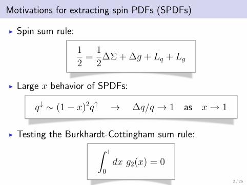
Motivations for extracting spin PDFs (SPDFs)

I Spin sum rule:

1

2=

1

2∆Σ + ∆g + Lq + Lg

I Large x behavior of SPDFs:

q↓ ∼ (1− x)2q↑ → ∆q/q → 1 as x→ 1

I Testing the Burkhardt-Cottingham sum rule:∫ 1

0

dx g2(x) = 0

2 / 26

How to extract SPDFs?

I SPDFs are extracted from cross section asymmetriesbetween different initial state polarizations.

I Inclusive DIS: e+N → e′ +X (In this talk)

I Semi-Inclusive DIS: e+N → e′ + h+X

I Inclusive Jet production: p+ p→ J +X

I Inclusive π0 production: p+ p→ π0 +X

I W boson production: p+ p→ W → l +X

3 / 26

How to extract SPDFs

I In practice the polarized data covers a small range in Q2

in comparison with unpolarized data.

I In order to maximally utilize the data, the JAM analysisset the cuts to Q2 ≥ 1GeV2 and W 2 ≥ 3.5GeV2.

I For such cuts the extraction of g1 and g2 is potentiallysensitive to:

I Finite Q2 corrections: TMC, HT

I Nuclear corrections for nuclear targets (especially for high-x).

4 / 26

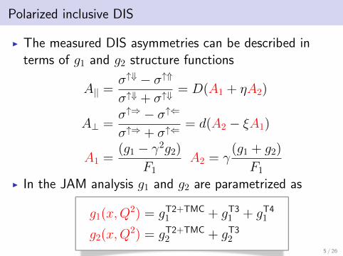
Polarized inclusive DIS

I The measured DIS asymmetries can be described interms of g1 and g2 structure functions

A|| =σ↑⇓ − σ↑⇑σ↑⇓ + σ↑⇓

= D(A1 + ηA2)

A⊥ =σ↑⇒ − σ↑⇐σ↑⇒ + σ↑⇐

= d(A2 − ξA1)

A1 =(g1 − γ2g2)

F1A2 = γ

(g1 + g2)

F1

I In the JAM analysis g1 and g2 are parametrized as

g1(x,Q2) = gT2+TMC

1 + gT31 + gT4

1

g2(x,Q2) = gT2+TMC

2 + gT32

5 / 26

Polarized inclusive DIS

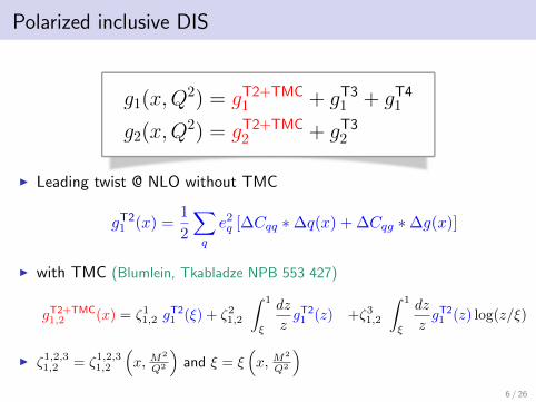
g1(x,Q2) = gT2+TMC

1 + gT31 + gT4

1

g2(x,Q2) = gT2+TMC

2 + gT32

I Leading twist @ NLO without TMC

gT21 (x) =1

2

∑q

e2q [∆Cqq ∗∆q(x) + ∆Cqg ∗∆g(x)]

I with TMC (Blumlein, Tkabladze NPB 553 427)

gT2+TMC1,2 (x) = ζ11,2 g

T21 (ξ) + ζ21,2

∫ 1

ξ

dz

zgT21 (z) +ζ31,2

∫ 1

ξ

dz

zgT21 (z) log(z/ξ)

I ζ1,2,31,2 = ζ1,2,31,2

(x, M

2

Q2

)and ξ = ξ

(x, M

2

Q2

)6 / 26

Polarized inclusive DIS

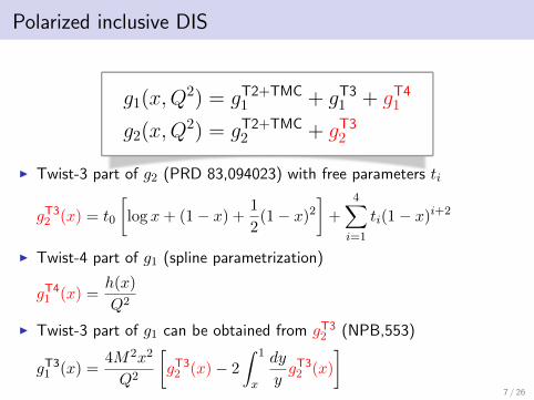
g1(x,Q2) = gT2+TMC

1 + gT31 + gT4

1

g2(x,Q2) = gT2+TMC

2 + gT32

I Twist-3 part of g2 (PRD 83,094023) with free parameters ti

gT32 (x) = t0

[log x+ (1− x) +

1

2(1− x)2

]+

4∑i=1

ti(1− x)i+2

I Twist-4 part of g1 (spline parametrization)

gT41 (x) =h(x)

Q2

I Twist-3 part of g1 can be obtained from gT32 (NPB,553)

gT31 (x) =4M2x2

Q2

[gT32 (x)− 2

∫ 1

x

dy

ygT32 (x)

]7 / 26

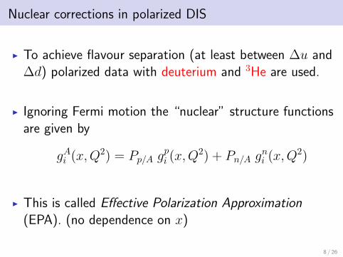
Nuclear corrections in polarized DIS

I To achieve flavour separation (at least between ∆u and∆d) polarized data with deuterium and 3He are used.

I Ignoring Fermi motion the “nuclear” structure functionsare given by

gAi (x,Q2) = Pp/A gpi (x,Q

2) + Pn/A gni (x,Q2)

I This is called Effective Polarization Approximation(EPA). (no dependence on x)

8 / 26

Nuclear corrections in polarized DIS

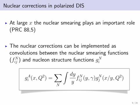
I At large x the nuclear smearing plays an important role(PRC 88,5)

I The nuclear corrections can be implemented asconvolutions between the nuclear smearing functions(fNij ) and nucleon structure functions gNi

gAi (x,Q2) =∑N

∫dy

yfNij (y, γ)gNj (x/y,Q2)

9 / 26

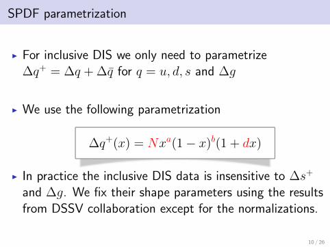
SPDF parametrization

I For inclusive DIS we only need to parametrize∆q+ = ∆q + ∆q for q = u, d, s and ∆g

I We use the following parametrization

∆q+(x) = Nxa(1− x)b(1 + dx)

I In practice the inclusive DIS data is insensitive to ∆s+

and ∆g. We fix their shape parameters using the resultsfrom DSSV collaboration except for the normalizations.

10 / 26

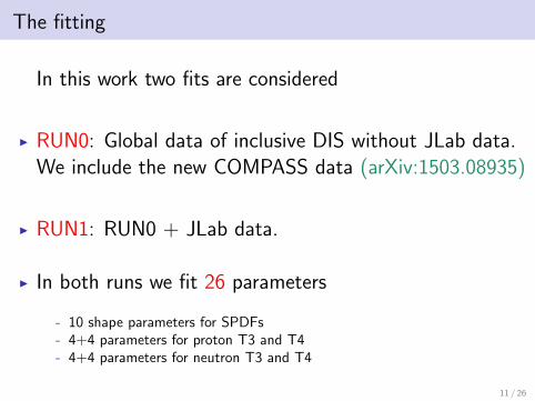
The fitting

In this work two fits are considered

I RUN0: Global data of inclusive DIS without JLab data.We include the new COMPASS data (arXiv:1503.08935)

I RUN1: RUN0 + JLab data.

I In both runs we fit 26 parameters

- 10 shape parameters for SPDFs- 4+4 parameters for proton T3 and T4- 4+4 parameters for neutron T3 and T4

11 / 26

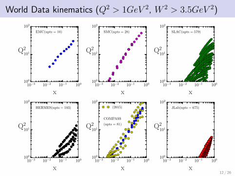
World Data kinematics (Q2 > 1GeV 2, W 2 > 3.5GeV 2)

10−3 10−2 10−1 100

x

100

101

102

Q2

EMC(npts = 10)

10−3 10−2 10−1 100

x

100

101

102

Q2

SMC(npts = 28)

10−3 10−2 10−1 100

x

100

101

102

Q2

SLAC(npts = 579)

10−3 10−2 10−1 100

x

100

101

102

Q2

HERMES(npts = 103)

10−3 10−2 10−1 100

x

100

101

102

Q2COMPASS

(npts = 81)

(2015)

10−3 10−2 10−1 100

x

100

101

102

Q2

JLab(npts = 675)

12 / 26

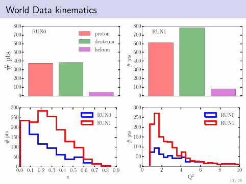
World Data kinematics

0

100

200

300

400

500

600

700

800

#p

ts

RUN0 proton

deuteron

helium

0.0 0.1 0.2 0.3 0.4 0.5 0.6 0.7 0.8 0.9x

0

50

100

150

200

250

300

#p

ts

RUN0

RUN1

0

100

200

300

400

500

600

700

800

#p

ts

RUN1

0 2 4 6 8 10

Q2

0

50

100

150

200

250

300

#p

ts

RUN0

RUN1

13 / 26

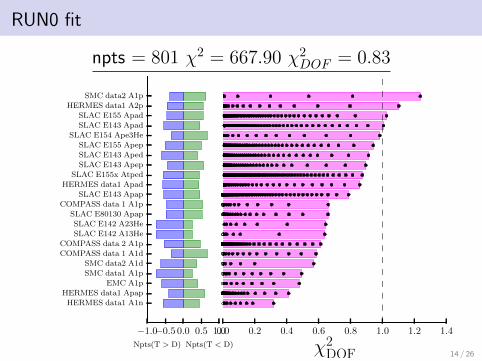
RUN0 fit

npts = 801 χ2 = 667.90 χ2DOF = 0.83

0.0 0.2 0.4 0.6 0.8 1.0 1.2 1.4

χ2DOF

−1.0−0.5 0.0 0.5 1.0

Npts(T > D) Npts(T < D)

HERMES data1 A1n

HERMES data1 Apap

EMC A1p

SMC data1 A1p

SMC data2 A1d

COMPASS data 1 A1d

COMPASS data 2 A1p

SLAC E142 A13He

SLAC E142 A23He

SLAC E80130 Apap

COMPASS data 1 A1p

SLAC E143 Apap

HERMES data1 Apad

SLAC E155x Atped

SLAC E143 Apep

SLAC E143 Aped

SLAC E155 Apep

SLAC E154 Ape3He

SLAC E143 Apad

SLAC E155 Apad

HERMES data1 A2p

SMC data2 A1p

14 / 26

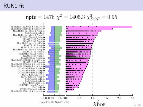
RUN1 fit

npts = 1476 χ2 = 1405.3 χ2DOF = 0.95

0.0 0.5 1.0 1.5 2.0 2.5

χ2DOF

−1.0−0.5 0.0 0.5 1.0

Npts(T > D) Npts(T < D)

JLabHallA E99117 1 Apa3HeHERMES data1 A1n

EMC A1pHERMES data1 Apap

SLAC E142 A13HeSMC data2 A1dSMC data1 A1p

SLAC E80130 ApapSLAC E142 A23He

COMPASS data 1 A1pCOMPASS data 2 A1pCOMPASS data 1 A1d

JLabHallA E06014 1 Ape3HeJLabHallA E06014 2 Apa3He

SLAC E143 ApapJLabHallA E06014 2 Ape3He

SLAC E155x AtpedSLAC E143 Apep

HERMES data1 ApadSLAC E143 Aped

JLabHallB eg1 dvcs 1 ApapSLAC E154 Ape3He

SLAC E155 ApepJLabHallB eg1b ApaDd

SLAC E155 ApadSLAC E143 Apad

HERMES data1 A2pJLabHallB eg1 dvcs 1 Apad

SMC data2 A1pJLabHallB eg1 dvcs 2 Apap

JLabHallA E99117 1 Ape3HeJLabHallA E06014 1 Apa3He

15 / 26

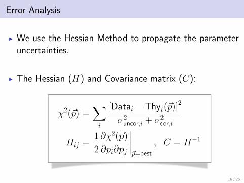
Error Analysis

I We use the Hessian Method to propagate the parameteruncertainties.

I The Hessian (H) and Covariance matrix (C):

χ2(~p) =∑i

[Datai − Thyi(~p)]2

σ2uncor,i + σ2

cor,i

Hij =1

2

∂χ2(~p)

∂pi∂pj

∣∣∣∣~p=best

, C = H−1

16 / 26

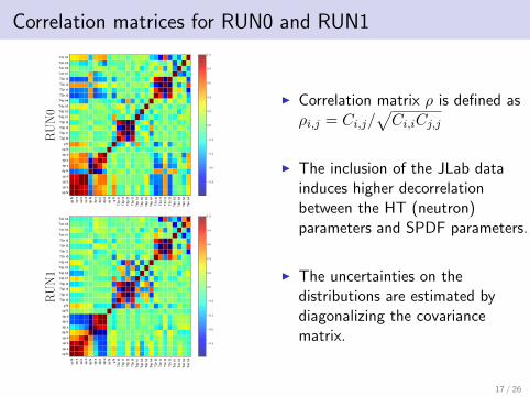
Correlation matrices for RUN0 and RUN1

upN

upa

upb

upd

dpN

dpa

dpb

dpd

spN

gN

T3p

t0T3

pt1

T3p

t2T3

pt3

T4p

h1T4

ph2

T4p

h3T4

ph4

T3n

t0T3

nt1

T3n

t2T3

nt3

T4n

h1T4

nh2

T4n

h3T4

nh4

up N

up a

up b

up d

dp N

dp a

dp b

dp d

sp N

g N

T3p t0

T3p t1

T3p t2

T3p t3

T4p h1

T4p h2

T4p h3

T4p h4

T3n t0

T3n t1

T3n t2

T3n t3

T4n h1

T4n h2

T4n h3

T4n h4

RU

N0

−0.8

−0.6

−0.4

−0.2

0.0

0.2

0.4

0.6

0.8

1.0

upN

upa

upb

upd

dpN

dpa

dpb

dpd

spN

gN

T3p

t0T3

pt1

T3p

t2T3

pt3

T4p

h1T4

ph2

T4p

h3T4

ph4

T3n

t0T3

nt1

T3n

t2T3

nt3

T4n

h1T4

nh2

T4n

h3T4

nh4

up N

up a

up b

up d

dp N

dp a

dp b

dp d

sp N

g N

T3p t0

T3p t1

T3p t2

T3p t3

T4p h1

T4p h2

T4p h3

T4p h4

T3n t0

T3n t1

T3n t2

T3n t3

T4n h1

T4n h2

T4n h3

T4n h4

RU

N1

−0.8

−0.6

−0.4

−0.2

0.0

0.2

0.4

0.6

0.8

1.0

I Correlation matrix ρ is defined asρi,j = Ci,j/

√Ci,iCj,j

I The inclusion of the JLab datainduces higher decorrelationbetween the HT (neutron)parameters and SPDF parameters.

I The uncertainties on thedistributions are estimated bydiagonalizing the covariancematrix.

17 / 26

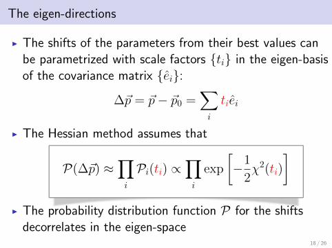
The eigen-directions

I The shifts of the parameters from their best values canbe parametrized with scale factors {ti} in the eigen-basisof the covariance matrix {ei}:

∆~p = ~p− ~p0 =∑i

tiei

I The Hessian method assumes that

P(∆~p) ≈∏i

Pi(ti) ∝∏i

exp

[−1

2χ2(ti)

]I The probability distribution function P for the shifts

decorrelates in the eigen-space18 / 26

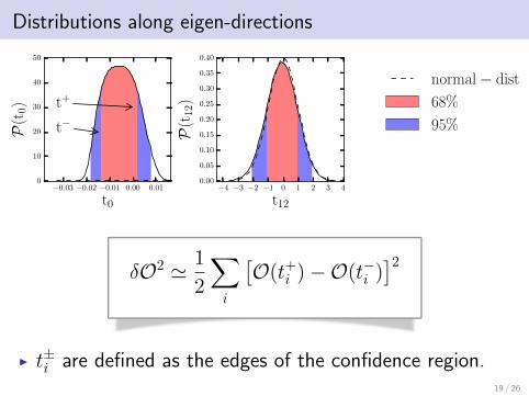
Distributions along eigen-directions

−0.03 −0.02 −0.01 0.00 0.01

t0

0

10

20

30

40

50

P(t

0)

t−t+

−4 −3 −2 −1 0 1 2 3 4

t12

0.00

0.05

0.10

0.15

0.20

0.25

0.30

0.35

0.40

P(t

12)

normal− dist

68%

95%

δO2 ' 1

2

∑i

[O(t+i )−O(t−i )

]2

I t±i are defined as the edges of the confidence region.19 / 26

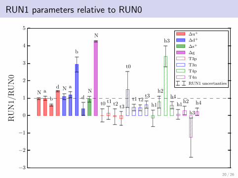
RUN1 parameters relative to RUN0

−3

−2

−1

0

1

2

3

4

5

RU

N1/

RU

N0

N a

b

d N a

b

dN

N

t0 t1 t2t3

t0

t1 t2t3

h1

h2

h3

h4

h1h2

h3

h4

∆u+

∆d+

∆s+

∆g

T3p

T3n

T4p

T4n

RUN1 uncertanties

20 / 26

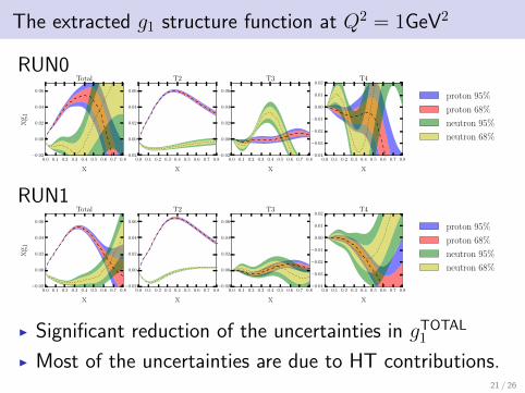
The extracted g1 structure function at Q2 = 1GeV2

RUN0

0.0 0.1 0.2 0.3 0.4 0.5 0.6 0.7 0.8

x

−0.02

0.00

0.02

0.04

0.06

xg1

Total

0.0 0.1 0.2 0.3 0.4 0.5 0.6 0.7 0.8

x

−0.02

0.00

0.02

0.04

0.06

T2

0.0 0.1 0.2 0.3 0.4 0.5 0.6 0.7 0.8

x

−0.02

0.00

0.02

0.04

0.06

T3

0.0 0.1 0.2 0.3 0.4 0.5 0.6 0.7 0.8

x

−0.04

−0.03

−0.02

−0.01

0.00

0.01

0.02T4

proton 95%

proton 68%

neutron 95%

neutron 68%

RUN1

0.0 0.1 0.2 0.3 0.4 0.5 0.6 0.7 0.8

x

−0.02

0.00

0.02

0.04

0.06

xg1

Total

0.0 0.1 0.2 0.3 0.4 0.5 0.6 0.7 0.8

x

−0.02

0.00

0.02

0.04

0.06

T2

0.0 0.1 0.2 0.3 0.4 0.5 0.6 0.7 0.8

x

−0.02

0.00

0.02

0.04

0.06

T3

0.0 0.1 0.2 0.3 0.4 0.5 0.6 0.7 0.8

x

−0.04

−0.03

−0.02

−0.01

0.00

0.01

0.02T4

proton 95%

proton 68%

neutron 95%

neutron 68%

I Significant reduction of the uncertainties in gTOTAL1

I Most of the uncertainties are due to HT contributions.21 / 26

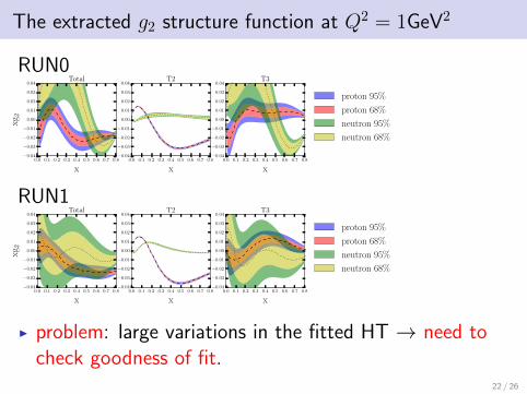
The extracted g2 structure function at Q2 = 1GeV2

RUN0

0.0 0.1 0.2 0.3 0.4 0.5 0.6 0.7 0.8

x

−0.04

−0.03

−0.02

−0.01

0.00

0.01

0.02

0.03

0.04

xg2

Total

0.0 0.1 0.2 0.3 0.4 0.5 0.6 0.7 0.8

x

−0.04

−0.03

−0.02

−0.01

0.00

0.01

0.02

0.03

0.04T2

0.0 0.1 0.2 0.3 0.4 0.5 0.6 0.7 0.8

x

−0.04

−0.03

−0.02

−0.01

0.00

0.01

0.02

0.03

0.04T3

proton 95%

proton 68%

neutron 95%

neutron 68%

RUN1

0.0 0.1 0.2 0.3 0.4 0.5 0.6 0.7 0.8

x

−0.04

−0.03

−0.02

−0.01

0.00

0.01

0.02

0.03

0.04

xg2

Total

0.0 0.1 0.2 0.3 0.4 0.5 0.6 0.7 0.8

x

−0.04

−0.03

−0.02

−0.01

0.00

0.01

0.02

0.03

0.04T2

0.0 0.1 0.2 0.3 0.4 0.5 0.6 0.7 0.8

x

−0.04

−0.03

−0.02

−0.01

0.00

0.01

0.02

0.03

0.04T3

proton 95%

proton 68%

neutron 95%

neutron 68%

I problem: large variations in the fitted HT → need tocheck goodness of fit.

22 / 26

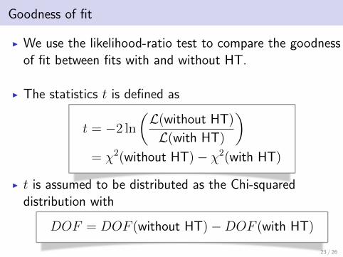
Goodness of fit

I We use the likelihood-ratio test to compare the goodnessof fit between fits with and without HT.

I The statistics t is defined as

t = −2 ln

(L(without HT)

L(with HT)

)= χ2(without HT)− χ2(with HT)

I t is assumed to be distributed as the Chi-squareddistribution with

DOF = DOF (without HT)−DOF (with HT)

23 / 26

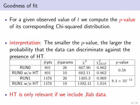
Goodness of fit

I For a given observed value of t we compute the p-valueof its corresponding Chi-squared distribution.

I interpretation: The smaller the p-value, the larger theprobability that the data can discriminate against thepresence of HT.

#pts #params χ2 χ2DOF p-value

RUN0 801 26 667.90 0.8620.58

RUN0 w/o HT 801 10 682.11 0.862

RUN1 1476 26 1405.3 0.9698.4× 10−12

RUN1 w/o HT 1476 10 1492.41 1.018

I HT is only relevant if we include Jlab data.

24 / 26

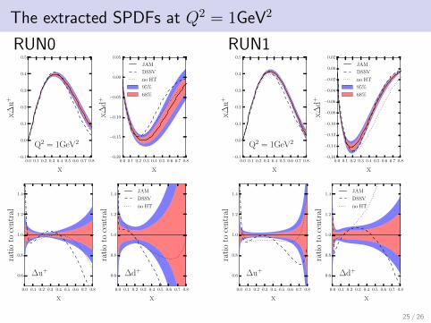
The extracted SPDFs at Q2 = 1GeV2

RUN0

0.0 0.1 0.2 0.3 0.4 0.5 0.6 0.7 0.8

x

−0.1

0.0

0.1

0.2

0.3

0.4

0.5

x∆u

+

Q2 = 1GeV2

0.0 0.1 0.2 0.3 0.4 0.5 0.6 0.7 0.8

x

−0.20

−0.15

−0.10

−0.05

0.00

0.05

x∆d

+

JAM

DSSV

no HT

95%

68%

0.0 0.1 0.2 0.3 0.4 0.5 0.6 0.7 0.8

x

0.6

0.8

1.0

1.2

1.4

rati

oto

cent

ral

∆u+

0.0 0.1 0.2 0.3 0.4 0.5 0.6 0.7 0.8

x

0.6

0.8

1.0

1.2

1.4

rati

oto

cent

ral

∆d+

JAM

DSSV

no HT

RUN1

0.0 0.1 0.2 0.3 0.4 0.5 0.6 0.7 0.8

x

−0.1

0.0

0.1

0.2

0.3

0.4

0.5

x∆u

+

Q2 = 1GeV2

0.0 0.1 0.2 0.3 0.4 0.5 0.6 0.7 0.8

x

−0.16

−0.14

−0.12

−0.10

−0.08

−0.06

−0.04

−0.02

0.00

0.02

x∆d

+

JAM

DSSV

no HT

95%

68%

0.0 0.1 0.2 0.3 0.4 0.5 0.6 0.7 0.8

x

0.6

0.8

1.0

1.2

1.4

rati

oto

cent

ral

∆u+

0.0 0.1 0.2 0.3 0.4 0.5 0.6 0.7 0.8

x

0.6

0.8

1.0

1.2

1.4

rati

oto

cent

ral

∆d+

JAM

DSSV

no HT

25 / 26

...

Conclusions

I An error propagation for global fits based on the Hessianmethod was discussed.

I The new JLab data conclusively favors the extraction ofthe polarized structure functions with HT contributions.

TODO:

I Inclusion of SIDIS and inclusive polarized Jets/pions.

I Extension of the global fit to include unpolarized PDFsfits.

26 / 26