ivm institute for environmental studies - deltares · ivm institute for environmental studies ......
TRANSCRIPT

IVM Institute for Environmental Studies
MAMPEC 3.0 HANDBOOK Technical Documentation
Bert van Hattum (IVM Institute for Environmental Studies)
Jos van Gils (Deltares)
Hidde Elzinga (Deltares)
Arthur Baart (Deltares)
Report R-14/33, edition August 2014 19 August 2014
IVM Institute for Environmental Studies
The development of the first version of MAMPEC (version 1.2, released in 1999) was commissioned by the Antifouling Working Group of the European Paint Makers Association (CEPE) as subcontract within the project "Utilisation of more environmental friendly antifouling products", sponsored by the European Commission (DG XI; Contract # 96/559/3040/ DEB/E2).Additional updates of the model (2002 v1.4; 2006 v1.6; 2008 v2.0; 2011 v3.0) and maintenance and helpdesk activities were sponsored by CEPE in the period (2001-2013). The release of MAMPEC-BW for ballast water was supported by GESAMP-BWWG and the International Maritime Organization (IMO).
IVM Institute for Environmental Studies VU University Amsterdam De Boelelaan 1087 1081 HV AMSTERDAM The Netherlands T +31-20-598 9555 F +31-20-598 9553 E [email protected]
Deltares P.O. Box 177 2600 MH DELFT The Netherlands T +31-88-335 8273 F +31-88-335 8582 E [email protected]
Copyright © 2014, Institute for Environmental Studies, Deltares All rights reserved. No part of this publication may be reproduced, stored in a retrieval system or transmitted in any form or by any means, electronic, mechanical, photo-copying, recording or otherwise without the prior written permission of the copyright holder
IVM Institute for Environmental Studies
MAMPEC 3.0 HANDBOOK
Contents
Preface and acknowledgement 5
1 Introduction 7
2 Installation and requirements 9
3 Structure of the model 13
4 Hydrodynamics and transport modelling 15
4.1 Tidal exchange 17 4.2 Horizontal exchange due to eddy in the harbour entrance 17 4.3 Density driven exchange 18 4.4 Submerged dam 19 4.5 Extra flushing flows 20 4.6 Non-tidal water exchange 21 4.7 Wind-driven exchange 22 4.8 Total calculated exchange volumes (m3/tide) 26 4.9 Hydrodynamic exchange mechanisms in open harbour and shipping lane
environments 27 4.10 Transport and dispersion modelling in DELWAQ 27 4.11 Water Characteristics 29
5 Emissions of antifouling compounds 31
5.1 Leaching rate 32 5.2 Underwater surface area 34 5.3 Shipping intensity 35 5.4 Non- service life and other emissions 37 5.5 Spatial distribution of emissions in MAMPEC 38
6 Chemical fate processes 41
6.1 Volatilisation processes 41 6.2 Sorption and sedimentation 42 6.3 Degradation processes 43 6.4 Sediment processes 49 6.5 Predicted concentrations 54 6.6 Fluxes and significance of processes 55 6.7 PEC profile outside harbour 56 6.8 Speciation 56 6.9 Default compounds and properties 60 6.10 QSAR options and sources for chemical property data 61
7 Application, validation and sensitivity 63
7.1 Validation exercises 63 7.2 Benchmarking the transport of substances within a harbour basin 66 7.3 Sensitivity 69
8 Application for Ballastwater 71
References 73
Annex A Version history 79


IVM Institute for Environmental Studies
MAMPEC 3.0 HANDBOOK 5
Preface and acknowledgement
MAMPEC is an easy-to-use integrated hydrodynamic and chemical fate model, originally developed to predict environmental concentrations for the exposure assessment of antifoulants in harbours, rivers, estuaries and open water. The model is also being used for exposure assessment in freshwater systems and discharges of chemicals in ballast water.
The development of the first version of the MAMPEC model (version 1.02 released in 1999) was commissioned by the Antifouling Working Group (AFWG) of the European Paint Makers Association (CEPE) as part of the project "Utilisation of more environ-mental friendly antifouling products", sponsored by the European Commission (DG XI; Contract # 96/559/3040/ DEB/E2).
Between 2002 and 2008 further updates of the model (version 1.4--2.5) were prepared for CEPE-AFWG for reasons of compatibility with upgrades of the Windows XP/VISTA/7 OS, inclusion of standard EU and OECD emission scenarios new functionalities (advanced photolysis module, non-tidal hydrodynamic exchange, sediment processes, import/export functions), and languages (Japanese). The model is recognized and used by regulatory authorities in EU, USA and other OECD countries.
In the most recent version 3.0 (2011) the user interface and software have been upgraded to meet current standards ( .net framework) and several new functionalities (multiple run options, analysis of chemical fate processes, new export options) and languages (Chinese, Spanish) have been added.
In 2011 a special version for ballast water (MAMPEC-BW) was developed for the International Maritime Organization (IMO) and Joint Group of Experts on the Scientific Aspects of Marine Environmental Protection (GESAMP) for the exposure assessment of chemicals in ballast water.
In this technical documentation we have described the model formulations and background information that was previously described in separate documents and reports.
The authors gratefully acknowledge the contributions of members of the CEPE Antifouling Working Group Review Team in the last decade: J. Hunter and G. Prowse (Akzo Nobel, International Coatings), M. Pereira (Hempel), A. Jacobson and D. Baur (Dow Chemicals (Rohm & Haas)), B. Fenn, P. Turley, J. Poppleton, R. Martin (Arch Chemicals), C. Mackie, K. Long (Regulatory Compliance Ltd) , S. Furtado, L. Jones (PPG), R. Wilmes and K. Schmidt (Lanxess), E. Berg and K. Gjerdevik (Jotun)


IVM Institute for Environmental Studies
MAMPEC 3.0 HANDBOOK 7
1 Introduction
MAMPEC is a steady-state 2D integrated hydrodynamic and chemical fate model, originally developed for the exposure assessment of antifouling substances (van Hattum et al., 2002, 2006). The first version of the model was developed in 1999 commissioned by the Antifouling Working Group (AFWG) of the European Paint Makers Association (CEPE / CEFIC) and co-sponsored by the European Commission (DG XI). Since then updates have been released sponsored by CEPE-AFWG in 2002 (v1.4) [1], 2005 (v1.6), and 2008 (v2.5) compatible with changing requirements of common operating systems (Win9X-NT-2000-XP-VISTA-Win7) and requirements of users and competent authorities. The model and support documentation has been distributed freely via the internet (http://www.deltares.nl/en/software/1039844/mampec/1039846).
The model predicts concentrations of antifoulants in generalised ‘typical’ marine environments (open sea, shipping lane, estuary, commercial harbour, yachting marina, open harbour). The user can specify: emission factors (e.g., leaching rates, shipping intensities, residence times, ship hull underwater surface areas), compound-related properties and processes (e.g., Kd, Kow, Koc, volatilisation, speciation, hydrolysis, photolysis, biodegradation), and properties and hydrodynamics related to the specific environment (e.g. currents, tides, salinity, DOC, suspended matter load, port dimensions). MAMPEC includes options for advanced photolysis modelling, incorporation of wind-driven hydrodynamic exchange, and other non-tidal exchange processes important for areas without tidal action or inland freshwater environments. Included are also service-life emission and other scenarios developed by an OECD-EU working group (OECD, 2004; ) and adopted by EU as the standard environmental emission scenarios to be used for evaluation of the biocides under the Biocidal Products Directive (BPD, Directive 98/8/EC) and the more recent Biocidal Product Regulation (BPR, Regulation (EU) 528/2012).
The model has been validated for a number of compounds (see section 7.1) and is today recognized by regulatory authorities in EU, USA, Japan, and other OECD countries. MAMPEC has been adapted, sponsored by IMO, to include the standard environment and emission scenarios for ballast-water as recommended by GESAMP.
The documentation of formulations and backgrounds in MAMPEC has been described in different reports issued with new updates (e.g. van Hattum et al., 1999, 2002, 2006; Baart et al., 2003; Boon et al., 2008), and with additional explanations in release notes or documents prepared for the Technical Meetings of competent European authorities for the Biocidal Products Directive. In this technical document we have compiled this scattered information into one single document.


IVM Institute for Environmental Studies
MAMPEC 3.0 HANDBOOK 9
2 Installation and requirements
This section contains instructions for the installation of MAMPEC version 3.0, a short explanation of the different screens and modules in the model, and instructions to setup and execute calculations with the model. Further instructions and background are given in the help files incorporated into the model, the technical reports and documentation distributed with the model, and the MAMPEC support website at http://www.deltares.nl/en/software
Minimum requirements: Pentium III with 256 MB memory. The Microsoft .NET Framework v3.5 should be present. Hard-disk usage is approximately 6 MB for the installer and 18 MB after installation. Recommended are Pentium IV and higher in combination with 1 GB memory.
Make sure you have the proper administrative rights to install the program, when using the installer, or consult your IT manager.
The program and documentation can be downloaded from the support website at Deltares (http://www.deltares.nl/en/software/1039844/mampec/1039846) .
The program can be installed in two different ways:
• by using the MAMPEC v3 installer (MAMPECSetup.msi) (recommended) or the setup file (MAMPECSetup.exe)
• by using a zip-file (MAMPECSetup.zip) and unzipping in any directory or drive, including USB-drive (advanced users)
The installer program will check if a previous version of MAMPEC 3.0 is present and ask first to remove the old version using the common <Add or Remove Programs> utility in the <Control Panel> of Win XP.
The installer will check if the .NET Framework is present. When the .NET Framework is not present, the installer will ask to install the .NET Framework. This can be downloaded from Microsoft at: http://www.microsoft.com/downloads/details.aspx?FamilyID=333325fd-ae52-4e35-b531-508d977d32a6&DisplayLang=en or via the Windows Update function. Installation of the .NET Framework may take some time (up to several minutes), depending on the speed of the internet connection.
The program will install itself in a proposed directory c:\Program Files\Deltares\MAMPEC 3. If necessary this can be changed to a different install directory. Confirm the proposed standard option or adapt to your own wishes. The program will create a desktop short cut and a start-menu item in the start menu (All Programs in XP).
The program only creates files and subdirectories in the indicated directory. No additional windows system files are added.
When prior versions of MAMPEC exist on the computer (e.g. version 1.6 or 2.5) these do not need to be removed, as long as version 3.0 is installed in a different directory.
For the installation with the zip-file it is sufficient to extract the contents in a directory created by the user on any drive (e.g. USB-stick). When the user does not have sufficient administrative rights to create a subdirectory within Program Files, it is recommended to install/unzip in the user directory. A shortcut to the desktop (to

IVM Institute for Environmental Studies
10 Installation and requirements
MAMPEC.exe in the installation directory) needs to be created manually. The program can also be run as a portable application from an USB-stick or external drive.
WARNING: Windows 2000 and Windows WP are not supported anymore by Microsoft. For users still working with Win2000: please do not use blanks in path names, this may give problems when not all required Windows 2000 Services Packs have been installed. Example: Do not install in ‘Program Files’ directory. We recommend in that case to use the suggested directory C:\MAMPEC or e.g. C:\MAMPECv3.
Compatibility issues
The program has been tested under various versions of Windows OS: Windows XP Windows Vista, and Windows 7. The different configurations of Service Packs (SP) and processor types tested are indicated in the Table below.
OS Version Service Packs 32 / 64 Bits
Windows XP Professional SP3 32 bit
Windows VISTA Professional SP2 32 bit
Windows 7 Professional SP1 32 / 64 bit
Home Premium SP1 32 bit
Windows 8 Home Premium 8.1 32 / 64 bit
Administrative rights
On most systems (Win7, Vista, Win 8) local administrative rights are needed to run an application for the first time. This could also be the case with MAMPEC. When this is needed you will get a message from Windows asking you to run the model as administrator and to login as administrator. In that case you need to contact an administrator and ask for the permission to run MAMPEC on your system.
When installing MAMPEC, make sure that it is installed in a directory where you (as user) have the system rights to execute, read, write, create and delete files. Usually this is the case in user directories (e.g. C:\Users\Username\) and public directories (e.g. C:\Users\Public\ ).
Regional and country settings for decimal separator
Regional settings: The model works with dots or commas as decimal separator depending on the regional country settings. The model was developed with the English (US) settings, as this is the standard in most of the scientific literature and inter-national computer programs. The program works with most of the regular default country settings. However, when the regional settings have been edited by local users, the program may not function properly in all cases. When MAMPEC detects possible problems a warning message is provided. In case of persisting regional settings-related problems, we recommend to use the English (US) settings. On some platforms rebooting after changing the settings may be necessary. Problems with regional settings can be detected by inspecting the proper representation of numeric data with commas and dots (e.g. in compound properties screen) or by examining the effect of variations before and after the decimal separator and resulting changes in related input boxes (e.g. the conversions between rate-constant and half-life values in the Compound screen)

IVM Institute for Environmental Studies
MAMPEC 3.0 HANDBOOK 11
Uninstalling
Uninstalling: For installations with the installer: MAMPEC v3.0 can be removed using the common <Add or Remove Programs> utility in the <Control Panel> of Win XP. For installations with the zip-file, it is sufficient to remove the directories in which the zip-file was extracted.


IVM Institute for Environmental Studies
MAMPEC 3.0 HANDBOOK 13
3 Structure of the model
The basic structure of the MAMPEC model consists of a central user interface (UI), from which data are entered to or retrieved from a database, sub models are run and calcu-lation results are presented. The UI guides the user via different panels, menus and screens, and helps to provide the required input settings for 1) environments; 2) compound properties, and 3) emission scenarios. The user supplied information and the results of the calculations are stored in a database, which is shielded from the user. Interaction with the database is through the UI in order to maintain integrity of the database. From the UI various hydrodynamic and chemical fate modules are called upon for the calculations of water quality and hydraulic exchange and transport processes (DELWAQ and SILTHAR programmed in Fortran). The calculations are exe-cuted on a user-defined grid basis. The UI results and export screens allows the user to compose the input for MAMPEC and to run its computational part, or view, print or file results from previous runs, and to export and import scenario and compound settings.
Each combination of environment, compound and emission scenario is assigned auto-matically a unique identifying label, in order to keep track of the different runs of the model. Basic sets of (read-only) default settings for prototype environments and default emission scenarios are provided for reasons of standardisation and can be used for comparisons between different compounds.
The central User Interface (UI) was written in Windows Visual Basic 4.0 for versions 1.0 – 2.5 and since MAMPEC version 3.0 in C# under the Microsoft .NET Framework v3.5.
As mentioned above, input parameter settings of default or user-defined scenarios and results of model runs are stored in a database. In previous MAMPEC versions (v2.5 and older) the Microsoft Office Access format (*.mdb) was used. In the current version of MAMPEC v3.0 the well-known open-source SQL format (SQLite; *.db) is being used. The database itself is not password protected. In order to safeguard integrity of the model settings of the different scenarios and model runs users are advised not to open or edit the original database files. The database files (Mampec.db or MampecBW.db for the ballastwater version) can be found under the \Resources subdirectory of the direc-tory where MAMPEC is installed). Using the import/export functions in the model, settings can be imported into the database from previous MAMPEC versions (v2.0, v2.5) or exported to other MAMPEC v3.0 installations. This allows the easy exchange of settings between different users and avoids errors with typing new settings. Results of the model runs do not need to be exchanged, as MAMPEC can easily rerun the different scenarios.
MAMPEC has been translated in Japanese and Chinese. Other languages can be added in the near future. The different languages can be selected with the ‘Language’ button in the top menu bar. For some languages a translated version of the manual has been prepared (Japanese, Chinese). Note that for proper display of the Japanese and Chinese characters the East Asian fonts need to be installed in the Windows operating system. In XP this can be set via the ‘Control Panel’ and ‘Regional and Language Options’ and the ‘Languages’ tab, where the option ‘Install files for East Asian languages’ needs to be checked. When these files need to be installed, it may be necessary to use the Windows installation files (available in the subdirectory ‘.\I386\LANG’ ) or to ask assistance from your IT department.


IVM Institute for Environmental Studies
MAMPEC 3.0 HANDBOOK 15
4 Hydrodynamics and transport modelling
In MAMPEC, four different generic types of environments can be specified. In the environment lay-out section the dimensions for these environments need to be provided. Below, the four generic types of environments are shown, and the applicable hydrodynamic exchange mechanisms are listed. These mechanisms will be discussed in detail in the next section.
Commercial and
Estuarine
Harbour
Marina Open Sea
Shipping Lane
Open Harbour
Hydrodynamic Exchange:
Tidal
Horizontal
Density
Flushing
Wind
Other non-tidal
Tidal
Horizontal
Density
Flushing
Wind
Other non-tidal
Current Current
For the harbour environments, the following input data need to be provided in the environment screen of MAMPEC:
• “General” information: latitude of the marine. • “Layout” information: spatial dimensions of the harbour and its surroundings. • “Submerged dam specification” to define harbour opening details. • Information to quantify the hydrodynamic exchange, in the “Hydrodynamics”,
“Wind” and “Flush” tables. • “Water characteristics” information. • “Sediment” information. For the open sea and open harbour environments, the “Submerged dam specification”, as well as the “Wind” and “Flush” tables are lacking, and the “Layout” and “Hydro-dynamics” tables are much simpler.
In the user manual (accessible from within the program) further guidance is provided for each of the parameters in the environment screen and the default scenarios provided with the model.
We recommend to use an open harbour environment only in the case that the jetties are absent or floating (see schematic representation above), so that there can be a longitudinal current perpendicular to the jetties. In the case that the jetties are closed, we recommend to use a harbour or marine type of environment with the distance Y1 equal to the length of the jetties.

IVM Institute for Environmental Studies
16 Hydrodynamics and transport modelling
In marine and estuarine waters, the exchange of water between a harbour basin and the water in front of the basin is caused mainly by three phenomena (Eysink, 2004 and references therein), that is by:
• Tidal filling and emptying; • the horizontal eddy generated in the harbour entrance by the passing main flow; • vertical circulation currents in the harbour generated by density differences
between the water inside and outside the basin.
(1) (2) (3)
Figure 4.1 Main phenomena responsible for the exchange of water in harbours: (1) tidal exchange, (2) horizontal exchange, (3) density driven exchange
For harbour basins in freshwater or in marine environments without strong tidal motion, other non-tidal exchange mechanisms may play a role, such as e.g. wind-driven exchange. In some cases the above picture is complicated by the extra effects of a water discharge through the harbour basin to the open water. On the one hand such a discharge has a positive effect by increasing the flushing of the harbour basin, but on the other hand it may reduce other water exchange mechanisms.
Most quick assessment models only incorporate an empirical exchange rate (REMA, EUSES, Simplebox) or use only the tidal exchange. The MAMPEC model is an exception as it incorporates all phenomena and allows for empirical exchange volumes as well. Most current true 3D models, such as Delft3D (Lesser et al., 2004; Gerritsen et al., 2003), Mike-3 (McClimans, 2000) or Telemac (Hervouet, 2000), incorporate all processes but require very experienced users with a high level of hydrological knowledge to use the models.
MAMPEC calculates the total water exchange volume (Ve , m3) as the sum of the tidal
prism (Vt) and the exchange volumes due to the horizontal eddy in the harbour entrance (Vh), due to density currents (Vd), wind-driven exchange (Vw), non-tidal exchange flow (Vnt) and the extra flush flow from within the harbour (Vef):
e t h d w nt efV V V V V V V= + + + + + (4.1)
These exchange volumes will be discussed in more detail in the next sections.

IVM Institute for Environmental Studies
MAMPEC 3.0 HANDBOOK 17
4.1 Tidal exchange
The exchange by the emptying and filling of the basin over a tidal period, i.e. the tidal prism can easily be determined as:
t bV Aη= (4.2)
where:
Vt = tidal prism of the harbour basin (m3)
η = tidal amplitude / height (m)
Ab = (storage) area of the basin (m2).
4.2 Horizontal exchange due to eddy in the harbour entrance
A current passing the entrance of a basin generates an eddy in this entrance (see Figure 1). There, steep velocity gradients generate an exchange of water by tur-bulence. Through this mechanism water from outside penetrates the eddy and from there further into the harbour and to the centre of the eddy.
The rate of water exchange by this mechanism depends on the flow velocity in front of the harbour basin, the size of the entrance and the tidal prism. The rate of “horizontal water exchange” can be approximated by the formula (Eysink, 2004):
1 0 2. . . .h tQ f h b u f Q= − (4.3)
Qh = rate of horizontal water exchange (m3/s)
f1, f2 = empirical coefficients depending on geometry of the basin
h = average depth of entrance (m) at mean seal level
b = width of entrance (m)
u0 = main flow velocity in front of the entrance (m/s)
Qt = filling discharge due to rising tide, h.b.utide (m3/s)
utide = tidal in and out flow velocities in the entrance. This formula is valid for rivers (Qt = 0) and in tidal areas during flood; Qh is almost negligible during ebb (Eysink, 2004). Hence in tidal areas, substitution of
0 cosh h tη ω= − and 0 0,max sinu u tω= , and integration over the flood period (t=0 to
T/2) yield the total volume per tide by horizontal exchange:
0,max1 0 2. . . .h t
uV f h b T f V
π= − (4.4)
where:
Vh = total water exchange volume per tidal period by horizontal exchange
h0 = mean depth in entrance relative to mean sea level
u0,max = maximum flow velocity during tidal period
T = tidal period
Vt = tidal prism of harbour.

IVM Institute for Environmental Studies
18 Hydrodynamics and transport modelling
In case the equation yields a negative value for Vh it means that the horizontal exchange does not contribute to the total water exchange, in which case Vh = 0. Typical values for the coefficients f1 and f2 are within ranges 0.01-0.03 and 0.1-0.25 respectively. MAMPEC v3.0 adopts the values f1 = 0.02 and f2 = 0.2.
In the absence of tide, MAMPEC uses the formula below:
1 0 0,. . .h avgV f h b u T= (4.5)
u0,avg = average flow velocity in front of harbour entrance
4.3 Density driven exchange
Exchange of water masses is also caused by density differences between the water inside and outside the harbour basin (Figure 4.2). This mechanism is very effective and, besides, it affects the entire basin while the mechanisms discussed above are restricted to the area near the entrance. The water exchange due to the density currents is reduced by the tidal filling or emptying of the harbour basin (Figure 4.2).
Figure 4.2 Schematized flow profiles indicating reduction of density induced exchange flow by tidal filling or emptying of basin.
Hence, the rate of exchange by density currents (no influence of horizontal exchange assumed) can be described by:
0 ( - ) 2d do t
h bQ u u= (4.6)
where the density induced velocity equals:
12
3 0dou f ghρρ
∆=
(4.7)
IVM Institute for Environmental Studies
MAMPEC 3.0 HANDBOOK 19
Qd = exchange rate due to density currents (m3/s)
udo = exchange velocity without influence of tidal in- and outflow
g = acceleration of gravity (m/s2)
ρ = density of water
Δρ = characteristic density difference
f3 = coefficient. Assuming linear harmonic relationships between the relevant hydraulic parameters, Eysink (2004) integrates the density induced exchange flow rate over a tidal cycle, which yields:
12
max4 0 0 5 - d tV f h b gh T f Vρ
ρ ∆
=
(4.8)
Vd = exchange volume per tide due to density currents (m3)
f4,f5 = coefficients. For estimates of f4 and f5 we refer to Eysink (2004). The parameter f4 depends on the size of the harbour. In a large harbour the average water density will hardly follow the density fluctuation of the water in front of the harbour. In case of a small harbour basin and/or strong density currents however, the density of the water inside the harbour will follow the density fluctuations outside. This results in a reduction of the characteristic density difference inducing the density currents. This effect is included in coefficient f4. This effect has been estimated theoretically on the basis of linear harmonic theory.
4.4 Submerged dam
The model offers an option to specify a submerged dam in the harbour entrance. This type of dam can be present in small harbours in areas with large tidal differences. The model cannot handle harbours with dams or locks, that prevent complete emptying at low tide, and that are open only several hours per day during high tide, such as e.g. in the Channel area. In this case we recommend to simulate this as an effective tidal range that matches the water level changes inside the harbour. Example: Sutton harbour (Plymouth, UK) has a tidal range of app. 5 m, a maximum harbour depth at high tide of 3.5 m and locks that close when the water depth in the harbour is 3 m. The effective tidal range then becomes 0.5 m.
The following parameters need to be specified in the environment screen:
Height of submerged dam
The height of the submerged dam (ηdam, m), measured from the bottom of the harbour.
Width of submerged dam
The width of the submerged dam (ψdam, m). Usually, this value is the same as the Mouth width of the harbour (b, m).

IVM Institute for Environmental Studies
20 Hydrodynamics and transport modelling
From these two parameters, two other quantities are derived:
Depth-MSL (mean sea level) of harbour entrance
Calculated field: the depth of the harbour entrance (h0, m) is calculated as follows:
0 0 damh H η= − (4.9)
where H0 equals the mean depth of the harbour basin.
Exchange area harbour mouth, below mean sea level
Calculated field: the exchange area of the harbour entrance (A0, m2) is calculated as
follows:
0 0 dam damA bH η ψ= − (4.10)
In older MAMPEC versions (v1.6 to v2.5), h0 was not a calculated field, and the user
had the freedom to specify a value of 0 0 damh H η≠ − . This was the case in the
standard OECD-EU Commercial Harbour environment. In older versions, h0 was specified as 10m, where H0 = 15m and ηdam = 0m. In the present version 3 of MAMPEC, this combination of values is no longer possible. In the standard OECD-EU Commercial Harbour environment, h0 = 10 m, H0 = 15 m and ηdam = 5 m. This does not affect the results of this standard scenario.
In future versions we plan to make the width of the dam equal to the harbour entrance width by definition (ψdam = b), for reasons of consistency. Since such a change inevitably would cause changes in the results of one or more standard scenarios, it has not been implemented yet. We will implement it simultaneously with any future major upgrade of MAMPEC or revision of the default scenarios.
4.5 Extra flushing flows
In some cases water is withdrawn from a harbour (e.g. for cooling water; intake harbour) or water is discharged into it (e.g. drainage water, small river). In one way or another this affects the water exchange rate of the harbour basin.
In MAMPEC, only the direct extra flushing as a result of such flows (Qef, m3/s) is
included:
ef efV Q T= ⋅ (4.11)
where:
Vef = water exchange volume due to extra flushing
T = tidal period. The effect such a flushing flow may have on other exchange mechanisms is considered a secondary process and therefore neglected.

IVM Institute for Environmental Studies
MAMPEC 3.0 HANDBOOK 21
4.6 Non-tidal water exchange
Under specific conditions of weak tides, small currents and no density differences, other physical processes can become important. Water exchange can be caused by:
• non-tidal water level changes; • wind-induced currents. Typically, non-tidal water level changes are connected to larger scale water level differences (1-100 km) often also caused by wind or wind gradients. Under wind-induced currents we refer to local effects only, implying that both phenomena are indeed complementary.
Both processes are implemented schematically in MAMPEC. For the derivation of suitable methods to quantify these exchanges a case study based on the Finnish Uittamo marina was executed (Baart et al., 2005), the main results of which are repeated here. In the case of the Uittamo marina, the tidal amplitude is zero, the density differences are zero and the flow velocity in front of the harbour is very low (1 cm/s). This means that the exchange mechanisms related to tides, currents and density differences are of small relevance and that other exchange processes should be considered.
To estimate the importance of non-tidal water level changes in this specific area, water level measurements at the Turku station (60°26' N 22°06' E, see Figure 4.3) have been analysed.
Figure 4.3 Location of water level measurements
Hourly water level measurements, together with the daily minimum and maximum values have been obtained from the Finnish Institute of Marine Research for a 5-year period (1998-2002). During that period the average daily difference between the lowest and highest water level was 14.4 cm. The minimum daily difference is 3 cm, the maximum 77 cm. Like the tide, non-tidal water level changes will result in a water exchange between the marina and the sea.
Based on the average daily difference an exchange volume can be estimated:
_ 24nt daily avg bTV h A= ∆ (4.12)
Vnt = exchange volume by non-tidal water level changes (per tidal period)
Δhdaily_avg = average difference between daily maximum and minimum water level

IVM Institute for Environmental Studies
22 Hydrodynamics and transport modelling
Ab = (storage) area of the basin (m2)
T = tidal period (h)
In this approach the maximum difference in water levels over a 24 hour period is taken and then normalized to the tidal period. It does assume that on average over 24 hours the water level fluctuates and approaches a maximum height difference only once. The water level changes are non-tidal and most likely caused by large scale wind and atmospheric pressure effects, which are relatively slow processes (i.e. scale of days, not minutes/hours). It is therefore expected that the frequency of water level fluc-tuations will be similarly slow. In order to validate this approach, the hourly water level measurements at Turku for 2002 (8759 data points) have been further analysed. Based on the daily minimum and maximum water levels the average daily water level differ-ence in 2002 was 14.3 cm. Based on the hourly measurements of the fluctuations in 2002 the daily average water level difference amounts to 17.7 cm. The difference between both values is small. The estimate based on the daily maximum difference seems therefore a reasonable approach. In the Turku case, the daily maximum difference approach slightly underestimates the actual exchange (20 %).
In MAMPEC, the daily non-tidal water level difference is a user-defined input item, used to estimate the non-tidal exchange volume. It should be noted that if one has reason to assume a much higher frequency of water level fluctuations, one should make a proper estimation, based on hourly measurements.
For the Uittamo marina, using the daily maximum water level difference, a non-tidal water exchange of 4,370 m3/tidal period was estimated.
4.7 Wind-driven exchange
For the wind-driven exchange a simplified estimation formula was derived and tested in Baart et al. (2005). The simplified formula was based on simulations with a detailed 3D model executed with Delft3D. The derivation and parameter estimation of the model in Baart et al. (2005) is repeated here for the sake of completeness.
When the wind blows over a water surface, the interaction of wind and water results in shear stresses at the water surface, which may be relevant for the exchange of water between the marina and the surrounding sea.
If the wind direction drives the water flow parallel to the harbour entrance, this results in a flow velocity which is included in the MAMPEC model as input. The selected setting for the Finnish marina of 0.01 m/s is a lower estimate, based on local current measurements which are in the order of several centimetres per second. The effect of this parallel flow is included in the other exchange mechanisms.
However, when the wind is perpendicular to the harbour entrance, the surface flow in the harbour would cause a bottom return flow. In order to estimate the effect of wind on the harbour exchange flow and to derive schematised formulations, a 3D model of the MAMPEC marina schematisation has been set up.
Detailed 3D model
A schematic 3D model has been set up to calculate the depth integrated exchange flow in a harbour basin as a result of inland wind and a minor alongshore current (0.01 m s-
1). The model is schematic in the sense that only the basic flow conditions were simulated. The water body has been assumed to be homogeneous and any eddies in the horizontal plane that may occur in the basin have not been verified. Furthermore,

IVM Institute for Environmental Studies
MAMPEC 3.0 HANDBOOK 23
some assumptions with respect to the wind setup along the open boundaries were made for running of the model (see below for details). The model was setup using Delft3D-FLOW (Delft Hydraulics, 2005).
The grid used is shown in Figure 4.4. The boundaries are far enough from the area of interest (the harbour entrance), so that any circulations that may appear along the open boundaries do not affect the solution. The grid size in the harbour is a uniform 14 m by 10 m. Further away from the area of interest the grid sizes increase.
Figure 4.4 Hydrodynamic grid of 3D model for wind-driven exchange
The model area has a uniform depth of 2.2 m. The bottom roughness is incorporated in the model by means of a Chezy bottom friction coefficient with a value of 65 m1/2
s 1.
The background flow in the model is 0.01 m s-1, flowing from the left to the right (using Figure 4.4 as a reference). This is done by prescribing this velocity on the right hand side boundary and prescribing the gradient of the water level on the left hand side open boundary (Neumann type boundary). On the upper boundary, a fixed water level is prescribed. The other boundaries are closed. Table 4.2 provides a summary of the boundary conditions used.
Table 4.2 Boundary settings of the 3D model
Boundary section Type Prescribed value
left water level gradient -0.486 • 10-8
right velocity (logarithmic) 0.01 m s-1 (depth averaged)
upper water level 1.81 •10-5 m (left) to 0.0 m (right)
lower closed -
Note: At the upper boundary section the water level is interpolated linearly from the left (1.81 •10-5 m) to the right (0.0 m).
For the vertical eddy viscosity, the k-epsilon turbulence closure model is used. In the horizontal plane, the Horizontal Large Eddy Simulation (HLES) feature of Delft3D is applied. This feature allows for the calculation of flow separation and eddy generation by sharp bends in the geometry.
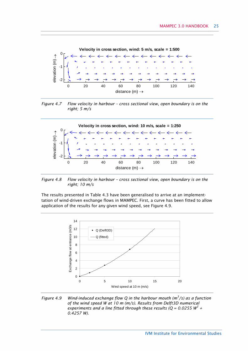
Four runs with corresponding wind speeds of 0.0 m s-1, 2.0 m s-1, 5.0 m s-1 and 10.0 m s-1 have been conducted with this model. The wind direction in those four runs was inland, perpendicular to the harbour entrance (“north” wind). In Figures 4.5 to 4.8 the cross sectional flow velocities are presented for the four scenarios. The bottom return
distance (m) →
dist
ance
(m) →
Hydrodynamic grid
0 500 1000 1500 2000 2500 3000 35000
500
1000

IVM Institute for Environmental Studies
24 Hydrodynamics and transport modelling
flow is clearly observed. The net depth averaged exchange flow has been calculated by integrating the fluxes through the interface between the harbour and the ambient water body. This has been done separately for the positive and negative fluxes, thereby yielding the exchange flows (see Table 4.3).
Table 4.3 Additional exchange flow at the harbour entrance due to inland wind perpendicular to the entrance
Wind speed at 10 m (m/s) Additional exchange flow at entrance (m3/s)
0.0 0.0
2.0 0.9
5.0 2.8
10.0 6.8
Figure 4.5 Flow velocity in harbour – cross sectional view, open boundary is on the right; 0 m/s
Figure 4.6 Flow velocity in harbour – cross sectional view, open boundary is on the right; 2 m/s
distance (m) →
elev
atio
n (m
) →
Velocity in cross section, wind: 0 m/s, scale = 1:1000
0 20 40 60 80 100 120 140
-2
-1
0
distance (m) →
elev
atio
n (m
) →
Velocity in cross section, wind: 2 m/s, scale = 1:1000
0 20 40 60 80 100 120 140
-2
-1
0
IVM Institute for Environmental Studies
MAMPEC 3.0 HANDBOOK 25
Figure 4.7 Flow velocity in harbour – cross sectional view, open boundary is on the right; 5 m/s
Figure 4.8 Flow velocity in harbour – cross sectional view, open boundary is on the right; 10 m/s
The results presented in Table 4.3 have been generalised to arrive at an implement-tation of wind-driven exchange flows in MAMPEC. First, a curve has been fitted to allow application of the results for any given wind speed, see Figure 4.9.
Figure 4.9 Wind-induced exchange flow Q in the harbour mouth (m3/s) as a function of the wind speed W at 10 m (m/s). Results from Delft3D numerical experiments and a line fitted through these results (Q = 0.0255 W2 + 0.4257 W).
distance (m) →
elev
atio
n (m
) →Velocity in cross section, wind: 5 m/s, scale = 1:500
0 20 40 60 80 100 120 140
-2
-1
0
distance (m) →
elev
atio
n (m
) →
Velocity in cross section, wind: 10 m/s, scale = 1:250
0 20 40 60 80 100 120 140
-2
-1
0
0
2
4
6
8
10
12
14
0 5 10 15 20
Wind speed at 10 m (m/s)
Exc
hang
e flo
w a
t ent
ranc
e (m
3/s
Q (Delft3D)
Q (fitted)

IVM Institute for Environmental Studies
26 Hydrodynamics and transport modelling
It has been assumed that similar exchange flows as calculated for inland wind, will also occur if the wind is directed from land to sea, again perpendicular to the marina entrance. Next, a correction is applied for the percentage of time that the wind is blowing from a direction perpendicular to the entrance (Fp).This factor depends on the local wind statistics and on the exact geometry of the harbour.
Furthermore, it has been assumed that the exchange flow depends linearly on the width of the harbour mouth (420 m in the case of the numerical experiments).
Thus, the formulation used by MAMPEC (version 2.0, 2.5, 3.0, 3.01) for the wind-driven exchange reads:
( )20.0255 0.4257420w pbV F W W T= ⋅ ⋅ + ⋅ ⋅ ⋅ (4.13)
where:
Vw = wind-driven exchange volume (m3)
Fp = fraction of time that the wind is perpendicular relative to the harbour mouth (-)
W = wind speed at 10 m (m/s)
b = width of the harbour entrance (m)
T = tidal period This formula to estimate the wind-driven exchange does not account for the depth of the marina. In cases where the depth is substantially smaller or larger than the 2.2 m of the Finnish model harbour (Baart et al. 2005), which was adopted to derive the formula, we recommend modifying the exchange flow proportionally to the ratio of the actual depth and 2.2. This can be done indirectly, preferably by changing the factor Fp
and may be implemented in future updates of MAMPEC.
The actual exchange due to wind effects also depends on the actual layout of the harbour and the free fetch area in front of the harbour. The way the harbour is schematised in the 3D model for the Uittamo marina (harbour entrance as wide as the harbour itself), leads to a maximal wind-driven exchange. Under less favourable con-ditions we can assume a smaller wind-driven exchange effect. Therefore, it is recom-mended to use conservative estimates for the speed of winds perpendicular to the harbour entrance.
4.8 Total calculated exchange volumes (m3/tide)
In the Environment input panel in MAMPEC, the calculated exchange volumes, according to the methods presented above, are listed. The total is expressed as m3/tidal cycle and as % / tidal cycle. For each of the contributing processes the contribution is presented in the same units (m3/tidal cycle and as % / tidal cycle).
Tidal due to the exchange filling and emptying by the tide
Horizontal due to horizontal eddy in harbour entrance generated by the river or other current
Density induced
vertical circulation due to density differences between freshwater and seawater
Wind-driven Due to circulation induced by wind when perpendicular to harbour entrance
Non-tidal Other non-tidal (measured) daily water level changes
Flushing flushing and vertical circulation from a small river discharging in the rear end of the harbour

IVM Institute for Environmental Studies
MAMPEC 3.0 HANDBOOK 27
4.9 Hydrodynamic exchange mechanisms in open harbour and shipping lane environments
In the open harbour and shipping lane environments, the hydrodynamic exchange is considered as a result of only the net flow. To this end, the user specifies an average flow velocity F in m/s and the model calculates the daily refresh rate as (F. 86400/L). 100% (expressed in % per day), where L is the length of the open harbour or shipping lane in m.
4.10 Transport and dispersion modelling in DELWAQ
4.10.1 Definition of grid
For the harbour type environments, MAMPEC creates a computational grid on the basis of the following assumptions (see Figure 4.10):
• the harbour part is modelled with a uniform 10 by 10 grid, which implies that the size of the grid cells equals Y1/10 by X2/10;
• the area in front of the harbour (marked “surroundings”), of dimensions Y2 by (X1+X2+X1) is covered with cells of equal size as in the harbour.
Figure 4.10 Simulation grid for a harbour type environment
The open harbour and shipping lane type environments are modelled with a grid of 20 by 10 cells. The cell dimensions are determined by the size of the modelled area: X by Y for the open sea and shipping lane, (X1+X2+X1) by Y for the open harbour.
4.10.2 Transport
MAMPEC carries out a simulation by solving the mass balance equation, (also known as transport equation or advection-diffusion equation) for the modelled compound. In two spatial dimensions this equation reads:
02 2
x y2 2
C C C C C = D u D v E St x x y y
∂ ∂∂ ∂
∂ ∂ ∂− + − + + =
∂ ∂ ∂ (4.14)
Y2
X3 X1
Y1
X2
Surroundings
Harbour
IVM Institute for Environmental Studies
28 Hydrodynamics and transport modelling
where:
C = total concentration (g/m3)
Dx, Dy = dispersion coefficients in two directions (m2/s)
E = emissions (g/m3/s)
S = source term representing decay and retention processes (g/m3/s)
u,v = velocity components in two directions (m/s)
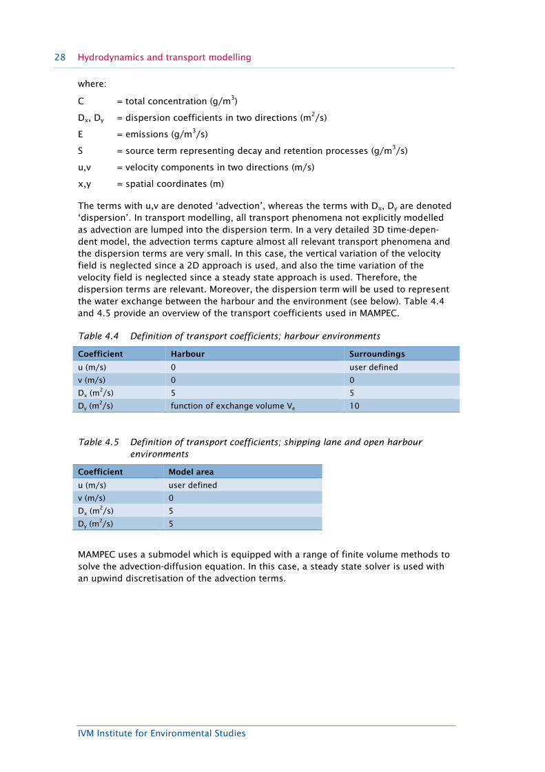
x,y = spatial coordinates (m) The terms with u,v are denoted ‘advection’, whereas the terms with Dx, Dy are denoted ‘dispersion’. In transport modelling, all transport phenomena not explicitly modelled as advection are lumped into the dispersion term. In a very detailed 3D time-depen-dent model, the advection terms capture almost all relevant transport phenomena and the dispersion terms are very small. In this case, the vertical variation of the velocity field is neglected since a 2D approach is used, and also the time variation of the velocity field is neglected since a steady state approach is used. Therefore, the dispersion terms are relevant. Moreover, the dispersion term will be used to represent the water exchange between the harbour and the environment (see below). Table 4.4 and 4.5 provide an overview of the transport coefficients used in MAMPEC.
Table 4.4 Definition of transport coefficients; harbour environments
Coefficient Harbour Surroundings
u (m/s) 0 user defined
v (m/s) 0 0
Dx (m2/s) 5 5
Dy (m2/s) function of exchange volume Ve 10
Table 4.5 Definition of transport coefficients; shipping lane and open harbour environments
Coefficient Model area
u (m/s) user defined
v (m/s) 0
Dx (m2/s) 5
Dy (m2/s) 5
MAMPEC uses a submodel which is equipped with a range of finite volume methods to solve the advection-diffusion equation. In this case, a steady state solver is used with an upwind discretisation of the advection terms.

IVM Institute for Environmental Studies
MAMPEC 3.0 HANDBOOK 29
Figure 4.11 Example of environment input screen
4.11 Water Characteristics
The settings for water characteristics and water quality parameters for most of the original default environment scenarios in MAMPEC since v1.0 (see description and explanation in van Hattum et al., 2002) were derived from data typical for the Southern North Sea along the Dutch coast. The values proposed for the first version of MAMPEC in 1999 were based on default values used in national models (MANS) for the Dutch part of the North Sea (Pagee et al., 1988), and derived from typical measured ranges in Dutch monitoring programmes for the port of Rotterdam (Rhine-Meuse estuary), Dutch coastal waters and values observed in shipping lanes in the southern part of the North Sea. The values for suspended particulate matter (SPM; 35 mg/L for harbours and 5 mg/L for the open sea) and for particulate organic carbon concentrations (POC; 1 and 0.3 mg/L respectively) are in line with data from older North Sea studies (Eisma and Kalf, 1987) and more recently from remote sensing studies of the same area as des-cribed in Eleveld et al. (2008). The organic carbon concentrations for the sediments (3 % for harbours and 0.5 % for the shipping Lane) are calculated from other parameters (the organic carbon content of SPM and degradation rate of organic carbon) since MAMPEC version 2.5 and are in line with results from the monitoring studies of Stronkhorst and van Hattum (2003).
The OECD-EU scenarios, used for regulatory purposes (see van de Plassche et al., 2004), were included since v1.6, and were derived from the older default MAMPEC scenarios.
Some typical values for the Dutch part of the North Sea and coastal area from long term monitoring programs are summarized in Table 4.6 and based on monitoring data obtained for several typical estuarine, coastal locations, and marine locations covering the time period 1990-2008. The data were kindly provided by the Dutch authorities (Rijkswaterstaat, Dutch Ministry of Transport, Public Works and Water Management). In Table 4.6 average values for the 18-year period are provided for SPM, POC, DOC, chlorophyll a, salinity, and sediment organic carbon. The data for Maassluis and Vlissingen can be seen as an example of the commercial harbour; Oosterschelde as an

IVM Institute for Environmental Studies
30 Hydrodynamics and transport modelling
example of the marina; Noordwijk (10 km from the coast)-as an indication for the shipping lane, and Terschelling (100 km from the coast) as typical for the open sea.
In Table 4.7 the current settings used in MAMPEC (v3.0) are indicated. In version 2.5 and before erroneous values for SPM and POC were present in the Default Shipping Lane and Default Open Sea scenarios.
Table 4.6. Dutch part of the North Sea and coastal area. Summary of water quality parameters (1990-2008) from the Dutch national monitoring programme and Donar database) for stations similar to the default and OECD-EU environment scenarios. Mean ± standard deviations; between brackets: number of observations
Commercial Harbour Marina
Shipping Lane Open Sea
Location: Maassluis
(Port of Rotterdam)
Vlissingen
(Western Scheldt)
Wissenkerke
(Oosterschelde)
Noordwijk
10 km from coast
Terschelling
100 km from coast
SPM (mg/L) 33 ± 36
(n=529)
47 ± 42
(n=696)
13 ± 11
(n=349)
6.6 ± 6.2
(n=821)
2.3 ± 1.9
(n=439)
POC (mg/L) 1.7± 0.9
(n=469)
1.4 ± 1.0
(n=526
0.6 ± 0.5
(n=350)
0.5 ± 0.5
(n=787)
0.2 ± 0.2
(n=438)
DOC (mg/L) 3.1 ± 0.9
(n=448)
2.0 ± 0.5
(n=458)
1.6 ± 0.4
(n=334)
1.5 ± 0.3
(n=723)
1.0 ± 0.2
(n=422)
Chlorophyll-a µg/L
6.7 ± 9.5
(n=459)
7.6 ± 8.4
(n=500)
5.2 ± 5.7
(n=344)
7.5 ± 10.2
(n=703)
1.1 ± 1.1
(n=434)
Salinity (psu) 2.0 ± 1.2
(n=39)
29.7 ± 1.9
(n=425)
31.7 ± 1.1
(n=357)
30.5 ± 1.5
(n=657)
34.6 ± 0.3
(n=265)
Sediment Org-C % 1.7 ± 2.3
(n=3)
1.8 ± 0.4
(n=11)
1.8 ±0.5
(n=11)
1.6 ± 1.6
(n=10)
1.3 ± 0.4
(n=30)
Table 4.7 Summary of current water quality parameters used in MAMPEC (v3.0)
OECD-Comm.
Harbour OECD Marina
OECD
Shipp. Lane
Default Comm.
Harbour
Default Estuar.
Harbour Default Marina
Default Shipp. Lane
Default Open Sea
SPM (mg/L) 35 35 5 35 35 35 5 5
POC (mg/L) 1 1 0.3 1 1 1 0.3 0.3
DOC (mg/L) 2 2 0.2 2 2 2 0.2 0.2
Chlorophyll-a µg/L
3 3 3 3 3 3 3 3
Salinity g/L 34 34 34 30 34 34 34 34
Sediment Org-C %
2.9 2.9 1.0 2.9 2.9 2.9 1.8 1.8
Temperature (oC)
15 20 15 15 15 20 15 15
pH (-) 7.5 8.0 8.0 7.5 7.5 8.0 8.0 8.0

IVM Institute for Environmental Studies
MAMPEC 3.0 HANDBOOK 31
5 Emissions of antifouling compounds
There are two key inputs of antifouling agents into harbours: emissions as a result of passive leaching from antifouling coatings on the underwater hulls of vessels visiting or moored within the harbour, and secondary emissions from biocide leaching from particulates that reach the harbour from maintenance and repair operations that may occur at the harbour side. The principal factor dictating the rate of these biocide releases is the passive leach rate, with biocide release from hull coatings in service (i.e. those coatings on the hull of the vessels present in the harbour) being the dominant release to the harbour. The magnitude of the biocide release is driven by a function of the release rate (LR in µg.cm-2.d-1) and the total underwater surface area (A in m2)
coated with the product (which in turn is controlled by the size and number of vessels treated with the coating).
Previous authors have proposed methods by which to determine this total emission. Various modelling studies (van Hattum et al., 2002) and the OECD emission scenario document (ESD) for antifouling products , written by a joint EU-OECD working group (van der Plassche and van der Aa, 2004), estimate the total emission (Etot in g.d-1) to a harbour according to formulas comparable to that of Eqn. 5.1, that is used in the MAMPEC model:
1 1( ) ( )
n n
tot i ib i b i im i mi i
E A N F LR A N F LR= =
= ⋅ ⋅ ⋅ + ⋅ ⋅ ⋅∑ ∑ in g.d-1 (5.1)
In which, Ai (in m2) represents the average underwater area of shipping category i, for n length categories; Nim and Nib represent the number (for category i) of moving ships and ships moored at berth in the harbour at any time of the day; Fi is the application factor expressed as the fraction of ships in category i treated with a specific anti-fouling product, and LRb and LRm are the compound and paint specific leaching rates (in g.m-2.d-1) of ships at berth or moving.
The total number of ships present in the harbour is the typical number of vessels present at any time of the day, which is derived from the number of port arrivals, manoeuvring, and residence time. For the commercial harbour and estuarine harbour an average residence time of 3 days is assumed for ships at berth, and the harbour manoeuvring time for arrival and departure is assumed to be 3 hours. Nib and Nim are derived from the total cumulative annual port statistics in the following way :
3365ib ibyN N= ⋅ (5.2)
0.125365im imyN N= ⋅ (5.3)
where:
Niby = total number of port visits per year in a specific length category.
Nimy = total number of ship movements in the port per year in the specific length class in the harbour.

IVM Institute for Environmental Studies
32 Emissions of antifouling compounds
5.1 Leaching rate
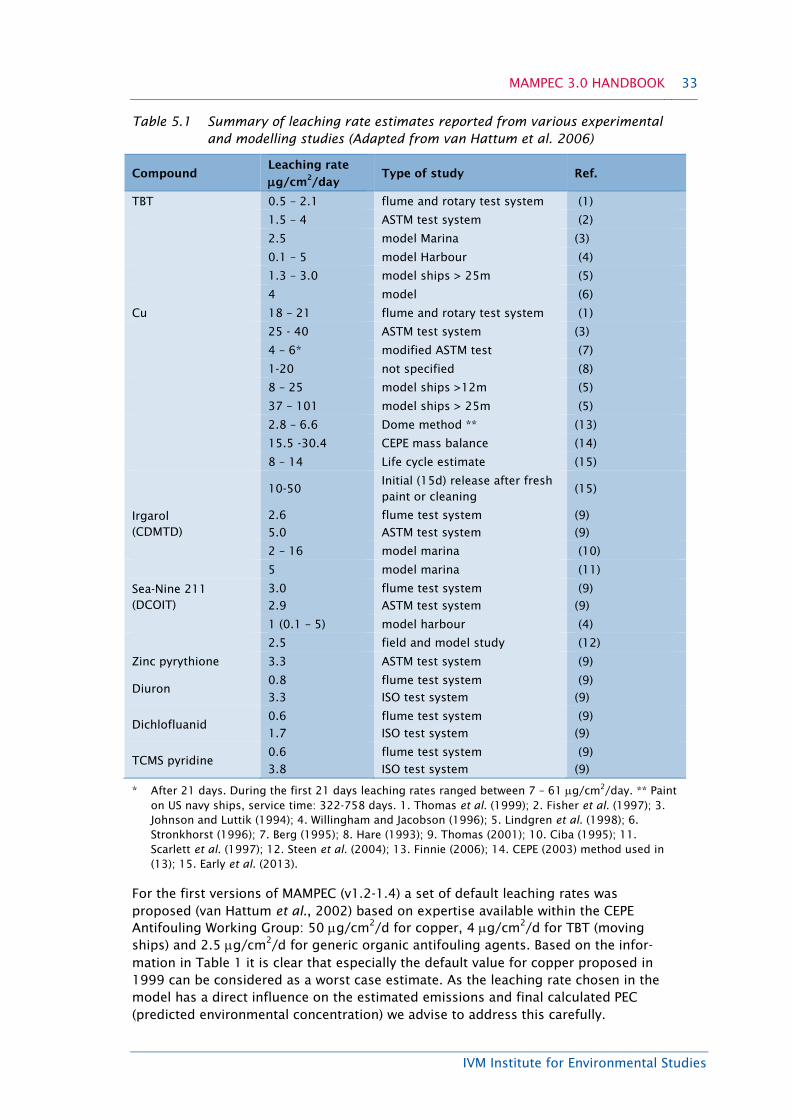
The leaching rate of a given biocide from a particular paint may vary depending on environmental factors, service time, and also the estimation method used. The careful selection of an appropriate estimation method is therefore important. A variety of published standards, calculation methods and practical methods to enable the estimation of leach rate are available. An excellent overview of the status of available methods and their relevance for emission estimation and environmental risk assess-ment is given in Finnie (2006). Reviews of factors affecting leaching rates and sum-maries of measured leaching rates can be found in Thomas and Waldcock (2000), Thomas (2001), van Hattum et al. (2006), and Finnie (2006). Measured or estimated leaching rates for different biocides, paint matrices, and measurement or estimation methods are summarized in Table 5.1 (adapted from van Hattum et al., 2002), and show a large variation (0.1 – 101 µg/cm2/day) .
Manufacturers usually conduct experimental determinations of leaching rates during the development en testing phases of new products, for instance, with test panels or rotating cylinders coated with the product and exposed to natural or semi-natural conditions. The results from these experimental studies cannot easily be translated to real-life leaching rates from ships to which the product is applied. Available ASTM (D5108-80) and ISO/DIS (15181-1,2) protocols have been criticized by various authors (Berg 1995, Thomas et al. 1998, Finnie 2006) and are usually considered as not suitable for application in risk assessment (Finnie 2006, EU Workshop 2006). Finnie (2006) described an in-situ method (Dome method) developed to determine actual leaching rates under field conditions.
In addition to this, mass balance based calculation approaches are being used. A mass-balance approach was followed in a study by Boxall et al. (2000). Worst case leaching rates were estimated based on the lifetime of the paint and national (UK) paint usage data. The overall estimates of Boxall and co-workers were in line with the ranges reported in Table 1. CEPE (the association of European Paint Makers) has proposed methods for use in environmental risk assessment that provide a conservative estimate of the release based upon the parameters of the dry paint film on the ship (CEPE, 2003). A more robust mass balance calculation method has recently been published by ISO nr 10890 (ISO 2010) which addresses concerns raised regarding certain aspects of the CEPE method and should be considered as the most appropriate mass balance method as it does not make any a priori assumptions about the way in which the biocide is released.
In principle, direct in-situ measurement methods provide the best estimate of environ-mentally relevant release rates, but there is currently no practical standardized method available for routine use. The use of calculation or laboratory methods may provide release rate estimates that do not reflect the true release rate under environmentally relevant conditions.
Except for the studies of Finnie (2006) and Steen et al. (2004) hardly any field studies on actual leaching rates or exposure from freshly painted ships have been published in the open literature. In various reviews good descriptions can be found of the different classes of biocidal antifouling paints and the dependency of the biocide leaching rate on the physical and chemical processes at the paint –(sea)water interface (Kiil et al. 2003, CEPE AFWG 1998, Omae, 2003).
Summarizing the available information from Table 1 it becomes evident, that for each of the compounds a broad range of leaching rate estimates is observed. Copper leaching rates usually are higher than for other compounds.
IVM Institute for Environmental Studies
MAMPEC 3.0 HANDBOOK 33
Table 5.1 Summary of leaching rate estimates reported from various experimental and modelling studies (Adapted from van Hattum et al. 2006)
Compound Leaching rate
µg/cm2/day Type of study Ref.
TBT 0.5 – 2.1 flume and rotary test system (1)
1.5 – 4 ASTM test system (2)
2.5 model Marina (3)
0.1 – 5 model Harbour (4)
1.3 – 3.0 model ships > 25m (5)
4 model (6)
Cu 18 – 21 flume and rotary test system (1)
25 - 40 ASTM test system (3)
4 – 6* modified ASTM test (7)
1-20 not specified (8)
8 – 25 model ships >12m (5)
37 – 101 model ships > 25m (5)
2.8 – 6.6 Dome method ** (13)
15.5 -30.4 CEPE mass balance (14)
8 – 14 Life cycle estimate (15)
10-50 Initial (15d) release after fresh paint or cleaning
(15)
Irgarol (CDMTD)
2.6
5.0
flume test system
ASTM test system
(9)
(9)
2 – 16 model marina (10)
5 model marina (11)
Sea-Nine 211 (DCOIT)
3.0
2.9
flume test system
ASTM test system
(9)
(9)
1 (0.1 – 5) model harbour (4)
2.5 field and model study (12)
Zinc pyrythione 3.3 ASTM test system (9)
Diuron 0.8
3.3
flume test system
ISO test system
(9)
(9)
Dichlofluanid 0.6
1.7
flume test system
ISO test system
(9)
(9)
TCMS pyridine 0.6
3.8
flume test system
ISO test system
(9)
(9)
* After 21 days. During the first 21 days leaching rates ranged between 7 – 61 µg/cm2/day. ** Paint on US navy ships, service time: 322-758 days. 1. Thomas et al. (1999); 2. Fisher et al. (1997); 3. Johnson and Luttik (1994); 4. Willingham and Jacobson (1996); 5. Lindgren et al. (1998); 6. Stronkhorst (1996); 7. Berg (1995); 8. Hare (1993); 9. Thomas (2001); 10. Ciba (1995); 11. Scarlett et al. (1997); 12. Steen et al. (2004); 13. Finnie (2006); 14. CEPE (2003) method used in (13); 15. Early et al. (2013).
For the first versions of MAMPEC (v1.2-1.4) a set of default leaching rates was proposed (van Hattum et al., 2002) based on expertise available within the CEPE Antifouling Working Group: 50 µg/cm2/d for copper, 4 µg/cm2/d for TBT (moving ships) and 2.5 µg/cm2/d for generic organic antifouling agents. Based on the infor-mation in Table 1 it is clear that especially the default value for copper proposed in 1999 can be considered as a worst case estimate. As the leaching rate chosen in the model has a direct influence on the estimated emissions and final calculated PEC (predicted environmental concentration) we advise to address this carefully.

IVM Institute for Environmental Studies
34 Emissions of antifouling compounds
For environmental risk assessment conducted to comply with a country’s particular regulatory requirements advice or guidance should be sought from the competent authority responsible for the administration of the regulation. In those cases where no guidance is given an appropriate method should be adopted for the scenario which the modeller is interested in. It is highly recommended that reader consults Finnie (2006), ISO (10890:2010), TM report of the workshop on leaching rates (2006), available RARs for antifoulants from the recent BPR review program, recent guidance from ECHA and stakeholders (CEPE) for guidance on estimating leaching rates.
5.2 Underwater surface area
A second parameter in the emission estimation (Eqn. 5.1), the total underwater area of ships painted with antifouling, depends on multiple factors, such as dimensions and shape of the various categories of ships, cargo load, residence time in the harbour, and various others. Some paint suppliers (IP 1999) have published general formulas for the estimation of the total underwater surface area (A) in order to estimate the required amount of paint needed to coat the hulls of recreational vessels. Simple dimensions are used to do this, such as overall length (L) or length at the waterline (LWL), width (W) or depth (D). For commercial ships comparable formulas have been used to derive the estimated surface area, which surprisingly show limited differences in average estimated surface area. A number of examples are given in Table 2.
Table 5.2 Simple formulas for first estimation of average underwater area.
Type of ship Formula Ref.
Recreational ships
Motor-launch (low draught) A = LWL . (W+D) IP (1999)
Sailing-yacht (intermediate draught)
A = 0.75 . LWL . (W+D) IP (1999)
Sailing yacht (deep keel) A = 0.5 . LWl . (W+D) IP (1999)
Generic motor-boat A = 0.85. Lwl . (W+D) Kovisto (2003)
Commercial ships
New York Harbour A = L . W . 1.3 Willingham & Jacobsen (1996)
Port of Rotterdam A = L.(W+D) + WD van Hattum et al. (2002)
Finnish harbours A = 0.95 . L . (0.8.(D+W)+W) Kovisto (2003)
Source: van Hattum et al. (2006)
The formula proposed by Willingham and Jacobson (1996) has been adopted for use in the emission estimation module in MAMPEC model for the default emission scenarios. Further refinements were made by applying average ratios between L and W (e.g. W as 14-15% of L) and L and D (e.g. D as 5% of L).
In the final ESD of the joint EU-OECD working group various approaches were compared and a more elaborate formula (Eqn. 5.4) was selected, which was derived from Finnish shipping data (Holtrop, 1977) referred to as the “Holtrop equation”. The latter approach yielded slightly (8-16%) higher estimates of the surface area for corres-ponding length classes compared to those used in the default scenarios in versions of MAMPEC before 2006 (version v1.2 and v1.4). In later versions of MAMPEC (v.1.6 and higher) the Holtrop equation is used in the OECD-EU default scenarios.

IVM Institute for Environmental Studies
MAMPEC 3.0 HANDBOOK 35
(2 ) [0.53 0.63 0.36( 0.5) 0.0013 ]m b mLA L D W C C CD
= + ⋅ + − − − (5.4)
where: A = submersed ship area, L = length of ship, D = depth, W = width,
Cm is an empirical shape factor (ranging from 0.95-0.98 , and used in the ESD as 0.975) for the curvature of the of the ship, and Cb is another empirical shape factor (ranging from 0.75-0.85, taken in the ESD as 0.8) for the underwater volume of the ship. The factors Cm and Cb are calculated according to the formulas:
( )m
mAC
W D=
⋅ (5.5)
( )d
bVC
L W D=
⋅ ⋅ (5.6)
In which: Am is the area of the main arch of the ship, i.e. the area of the biggest cross-section of the ship, which is in general in the middle of the ship, and Vd is the underwater volume of the ship (displacement). D and W are similar as in formula 5.4
The uncertainty in the estimation of the painted and submersed surface area can be significant. In the technical report for MAMPEC version 1.4 (van Hattum et al. 2002) results were shown of a statistical survey of paint-usage data in relation to ship dimensions (DWT) from a large paint supplier for 300 ships and covering 9 of the 25 main Lloyds shipping categories. . It was concluded that predicting submersed surfaces with simple generic regression formulas as shown in Table 5.2 may result in deviations up to several 100% below or above actual measured surface areas. Acknowledging the uncertainties, the OECD-EU commission advised to work with one uniform approach and to make use of the more accurate Holtrop equation( Eqn. 5.4). As noted above in the leaching rate section, for specific environmental risk assess-ments conducted to comply with a country’s particular regulatory requirements advice or guidance should be sought from the competent authority responsible for the administration of the regulation. In those cases where no guidance is given an appropriate method should be adopted for the scenario which the modeller is interested in. For most purposes the OECD scenarios can be considered to be appropriate where no clear guidance or data is available for dimensions of the vessel categories of interest.
5.3 Shipping intensity
A third set of parameters in Eqn. 5.1, the numbers of ships present in the port area (moving and moored) can be obtained from various sources, such as on-line port statistics from local port authorities or branch organizations such as the International Association of Ports and Harbours (IAPH), commercial suppliers (Lloyds Register Ltd), or trade oriented studies (ISL, 1997). Although traffic intensities and port arrivals are monitored on a large scale in European waters, there still is no structured and aggre-gated reporting system, especially for estimations of traffic intensities in open and coastal waters. Another problem is caused by the differences among harbours in reported dimensions and shipping types, such as length, depth, dead-weight tonnage (DWT), gross tonnage (GRT/GT), net tonnage (NRT/NT), compensated tonnage (CGT), cargo landed, number of containers, or economic parameters, such as revenue tons.

IVM Institute for Environmental Studies
36 Emissions of antifouling compounds
For the first version of MAMPEC (v 1.2), which appeared in 1999 available port statistics of Rotterdam and other harbours from around 1996 were used. The deri-vation was described in van Hattum (2002) and van Hattum et al. (2006) and is presented here briefly as it may give guidance to users in creating local or specific emissions scenarios.
The average number of port arrivals in some main European ports (ISL, 1997) varied in 1996 between approximately 4,400 ships per year for Helsinki (Finland) to more than 25,000 per year for Piraeus (Greece) and Rotterdam (Netherlands). In the first versions of the MAMPEC model (v1.2-v1.4) the shipping intensities and ship dimensions in the port of Rotterdam and the North Sea shipping lanes along the Dutch coast were used as a basis for the default emission scenarios for commercial sea going vessels. Rotterdam was one of the world’s biggest harbours and the North Sea shipping lane at that time had the highest numbers of passing ships. Both were considered as realistic worst case situations for the EU and worldwide.
Table 5.3. Original default emission scenarios in MAMPEC (v1.2-3.0). Indicated are average underwater surface area and number of ships moving (Nm) or at berth (Nb) for the different length classes.
Length class (m)
Surface area (m2)
Shipping Lane
Open Sea
Commercial Harbour
Estuarine Harbour
Marina
Nm Nm Nb Nm Nb Nm Nb
<50 22.5 - - - - - - 299
50 – 100 450 3.9 0.095 57 0.75 11 1.8 -
100 – 150 3,061 1.7 0.04 25.5 2.16 5 0.4 -
150 – 200 5,999 1.6 0.04 24.5 2.05 5 0.4 -
200 – 250 9,917 0.4 0.01 5.5 0.5 1 0.1 -
250 – 300 14,814 0.5 0.01 7.5 0.6 2 0.1 -
300 – 350 22,645 0.1 0.002 1.5 0.15 - - -
Estimated emission* (g.d-1)
755 154 11257 973 2245 173 168
* Of compound with a leaching rate 2.5 µg/cm2/day and 100% application of product. Source: van Hattum et al. (2002)
The default commercial harbour environment in version 1.2 - 2.5 had a size (surface area) of approximately 50% of that of the Rotterdam harbour. For the emission scenario of the default commercial harbour approximately one third the number of port arrivals of Rotterdam was taken as a basis. The numbers of moving (Nm) and moored ships at berth (Nb) were estimated according to Eqn 5.2 and 5.3. For further details and guidance about the derivation of the original default scenarios and the data for the port of Rotterdam the reader is referred to van Hattum et al. (2002) and (2001), both available at the support site of MAMPEC. Settings of the MAMPEC default emission scenarios are indicated in Table 5.3. The approach of the emission scenarios as endorsed by the OECD-EU working group and adopted as suitable for emission scenarios under the BPD.
The OECD-EU (PT-21) emission scenario document (van der Plassche and van der Aa, 2004) gives a detailed account of how the proposed default scenarios for regulatory exposure assessments were derived. A similar approach was used with different settings for the calculations of the number of ships and submersed surface areas (see

IVM Institute for Environmental Studies
MAMPEC 3.0 HANDBOOK 37
previous sections). The default settings for painted surface area and numbers of ships of the OECD-EU scenarios (present in MAMPEC versions v1.6 and higher), and the old default scenarios (present in all versions) are summarized in Table 5.3 and Table 5.4.
Table 5.4. OECD-EU Emission scenarios in MAMPEC. Recommended default service-life emission scenarios for antifoulings in Europe (Biocide Product Directive) and other OECD countries. Indicated are average underwater surface area and number of ships moving (Nm) or at berth (Nb) for the different length classes.
Length class
(m) Surface area (m2)
OECD-EU
Shipping Lane
OECD-EU
Commercial Harbour
OECD-EU
Marina
Nm Nb Nm Nb
<50 31 - - - 500
50 – 100 1,163 3.9 11 1.8 -
100 – 150 3,231 1.7 5 0.4 -
150 – 200 6,333 1.6 5 0.4 -
200 – 250 10,469 0.4 1 0.1 -
250 – 300 15,640 0.5 2 0.1 -
300 – 350 21,844 0.1 - - -
Estimated emission*
(g.d-1) 724 2303 192 345
* of compound with a leaching rate 2.5 µg/cm2/day and 90% application of product. Source: van der Plassche and van der Aa (2004)
Little information is available on the application factor of a product (Fi ), which constitutes the fourth parameter in Eqn.1. In general, market share information of specific products is confidential, but it is clear that this type of information is crucial for a proper estimation of the emissions. With currently existing differences in admission policies and regulation between countries, this may even vary on a country scale. Especially for the categories of smaller ships (<25 m), where antifouling pro-ducts tend to be more tightly controlled. In the EU-OECD emission scenario document (a worst case approach with values of 0.9 – 0.95 for Fi is recommended. For the original default MAMPEC scenarios present in a worst case of 1.0 was adopted.
5.4 Non- service life and other emissions
Other important emissions of antifouling compounds may occur from maintenance, repair, new buildings, removal and other activities. These so called non-service life emissions, in the form of e.g. paint dust or particles may constitute important local sources of antifouling compounds. In addition to the in-service life emissions already present in previous MAMPEC versions it is possible in v 3.0 to include non-service life emissions, related to new building, paint application, maintenance, repair, and removal operations, as specified in the OECD-EU PT-21 document (van der Plassche and van der Aa, 2004). In these scenarios emissions are subdivided in commercial shipping and recreational boats respectively and the last sector is further divided into emissions related to professional or non-professional activities.
In MAMPEC v3.0 the local emissions to water can be specified for different life stages (New building, Maintenance & repair, Removal) of the paint on both commercial ships and pleasure crafts. All the formulae specified in the OECD-EU PT-21 Document have

IVM Institute for Environmental Studies
38 Emissions of antifouling compounds
been implemented as described in van der Plassche and van der Aa (2004), to which we refer for further explanation of the prescribed procedures. The local emissions in g/day calculated according to OECD-EU PT-21 are emissions occurring during the specific painting or docking period. In MAMPEC these temporary emission rates have been extrapolated to annual average emission rates in g/day in order to obtain dimensions comparable to the in-service life emissions of moored and moving ships.
The following (sub)scenarios for non-service life emissions are considered:
Professional Non-professional
Commercial ships New building
Maintenance and repair
Removal
Pleasure crafts Maintenance and repair Maintenance and repair
Removal Removal
For both commercial ships and pleasure crafts structured input-fields and simple submenus are present to guide the estimation of the emissions. Additional submenus are present for calculation of the total emissions and analysis of the different contributions.
As there are at present no regulatory prescribed settings for non-service life emissions, no default values are currently included in MAMPEC v3.0. For specific assessments conducted to comply with regional or local requirements advice or guidance should be sought from the competent authority responsible for the administration of the regulation.
5.5 Spatial distribution of emissions in MAMPEC
In the Commercial or Estuarine Harbour and Marina type of environments, the emissions are distributed as follows:
• Emissions from ships at berth are distributed over the last row of cells along the back side of the harbour (10 cells);
Surroundings
Harbour

IVM Institute for Environmental Studies
MAMPEC 3.0 HANDBOOK 39
• Emissions from moving ships are divided over all cells in the harbour or marina (10x10 cells)
• Emissions from application and removal (“other emissions”) are distributed over the last row of cells along the back side of the harbour (10 cells).
In the Open Sea and Shipping Lane type of environments (20x10 cells) the emissions are from moving ships only and are distributed over the centre line of the environment in a longitudinal direction. The emissions are distributed over the 3 central rows.
In the Open Harbour type of environment, the emissions are situated along the harbour (section indicated by X2), in the second row of cells counted from the land side. The number of cells with emissions depends on the values of X2, Y and X1.
Shipping Lane / Open Sea
Open Harbour
Surroundings
Harbour


IVM Institute for Environmental Studies
MAMPEC 3.0 HANDBOOK 41
6 Chemical fate processes
The mass balance equation for a compound present in the water column is discussed in section 4. This equation (Eqn. 4.14) contains a source term S representing settling, volatilisation and decomposition. In particular:
, , snp w v df w w p p dfw w d w
vS f C r f C r f C r f Ch
= −− − − (6.1)
where:
h = water depth (m)
Cw = total concentration in the water column (g.m-3)
fdf = freely dissolved fraction (-)
fp = fraction adsorbed to suspended particulate matter (-)
rv = volatilisation rate (day-1)
rw,d = overall first order decomposition rate in the water column for the freely dissolved fraction (day-1)
rw,p = overall first order decomposition rate in the water column for the fraction in particles (day-1)
Ss = concentration of suspended solids (g.m-3)
vsn = net settling velocity (m.day-1) The dissolved fraction fdf is derived from the partitioning of a substance between water, dissolved organic matter and (organic) suspended matter. Not only dissolved fractions, but also particulate fractions are deduced using partition coefficients (see following section).
6.1 Volatilisation processes
The volatilisation rate rv is a function of substance and compartment specific coefficients, according to:
( )
1
1
1 1 .v
l a g
rk H k
h
−
= +
(6.2)
( )2
1 273.15a
aa
HHR T
=+
(6.3)
in which:
h = depth of water column (m)
Ha1 = dimensionless Henry's constant at average temp. ((mol.m-3).(mol.m-3)-1)
Ha2 = Henry's constant at average ambient temperature (Pa.m3.mol-1)
kg = mass transfer coefficient in the gas film (m.d-1), compartment specific

IVM Institute for Environmental Studies
42 Chemical fate processes
kl = mass transfer coefficient in the liquid film (m.d-1), compartment specific
R = gas constant (8.3 Pa.m3.mol-1.oK-1)
Ta = average ambient temperature (10 oC) The volatilisation rate rv is a function of substance related parameters (Henry’s constant) and compartment specific variables (depth, temperature, gas-water mass transfer coefficients). :
6.2 Sorption and sedimentation
Partitioning among the dissolved and particulate phases affects the loss and distribution of a substance as well as the exposure of organisms to this substance. Partitioning is formulated according to the equilibrium concept of partition coefficients. The total concentration of a modelled substance of an organic nature is the sum of three contributions:
( ) w poc doc df wC f f f C= + + (6.4)
in which:
Cw = total concentration (g.m-3)
fdf = freely dissolved fraction (-)
fdoc = fraction adsorbed to dissolved organic matter (-)
fpoc = fraction adsorbed to the organic part of (suspended) matter (-) All organic matter is expressed in amounts of carbon. The fractions are derived from a partition coefficient defined according to:
.p
df w
CP
f C= (6.5)
in which:
Cp = particulate concentration (g.g-1 OC)
P = partitioning coefficient (m3.g-1 OC = 10-6 l.kg-1 OC) The organic carbon-based partitioning coefficient (P) is usually available as Koc (l.kg-1), the conversion of which into P requires a multiplier of 10-6. In the literature, various QSAR relationships are described to estimate Koc on the basis of the octanol-water partition coefficient (Kow; l.kg-1), such as e.g. Karickhof et al. (1991); Sabljic and Güsten (1995).
The different fractions for an organic substance follow from equations 6.6-6.10:
1 1 df
toc
fPC
=+
(6.6)
( ) 1 pocpoc df
toc
Cf f
C= − (6.7)
IVM Institute for Environmental Studies
MAMPEC 3.0 HANDBOOK 43
( ) 1 doc docdoc df
toc
X Cf fC
= − (6.8)
poc oc sC f S= (6.9)
toc poc doc docC C X C= + (6.10)
in which:
Cdoc = dissolved organic carbon concentration (g OC.m-3)
Ctoc = total organic carbon concentration (g OC.m-3)
foc = fraction organic carbon in suspended solids
Ss = (suspended) sediment concentration (g.m-3)
Xdoc = sorption efficiency relative to particulate organic carbon (-);in MAMPEC a value of 0.1 is assumed according to Farrington et al. (1989)
Combining the fractions with the total concentration yields the individual probable exposure concentrations (PEC) in water and particulate matter. Similar formulations can be used for metals, but then sorption is considered relative to the total mass of (suspended) sediment instead of its organic part.
The fraction of the compounds adsorbed to SPM is removed from the water column by settling, as described by the equation listed above. The process of sedimentation is formulated in MAMPEC using a single net settling velocity (vsn in m.day-1), accounting for both sedimentation and resuspension. This is further explained in the section “Sediment processes” and “Estimation of net sedimentation rate”.
6.3 Degradation processes
The overall first order decomposition rate in the water column rw (day-1) is derived from the rate constants specified for photolysis, hydrolysis and other abiotic processes, and biodegradation (aerobic and anaerobic), if all of these contributions are separately known. rw = rhydrolysis + rphotolysis + rbiodegradation (6.11) The user needs to provide reliable data. If only information is available on overall degradation, than the equivalent rate constant can be entered under any of the categories. Hydrolysis and biodegradation may be assumed to take place evenly distributed over the whole water column. It should be noted that most degradation rates can be scenario-specific. As an example, the hydrolysis rate constant of dichlofluanid is known to increase with pH and temperature (Bayer, 2002). The photolysis rate constant is dependent on both compound and environment related factors and varies with water depth, time of the day, and season. MAMPEC offers an option to help estimating reliable photolysis rate constants.
All three clusters of degradation processes can be specified separately for the water phase (acting on the freely dissolved fraction) and for the SPM / sediment phase (acting on the fraction sorbed to SPM). The fraction sorbed to DOC does not undergo any degradation.

IVM Institute for Environmental Studies
44 Chemical fate processes
6.3.1 Photolysis
The contribution of photolysis is of importance for a number of compounds during day time and for water depths with sufficient light penetration, for example in open sea areas with a high intensity of incident light and a low turbidity as often encountered in (sub)tropical waters. The rate of photolysis is dependent on many both compound and environment-specific factors, such as e.g. wavelength dependent absorption and quan-tum yield of the compound, time of year, latitude, depth, atmospheric conditions and several factors which affect the light transmission characteristics of the water body, e.g. concentration of DOC, SPM, and chlorophyll (Mill, 2000). Proper handling of photolysis can only be executed in 3D models. In the WAQ module of Delft3D (Delft Hydraulics, 2005), various libraries and protocols are provided for the treatment of photolysis. The well-known exposure assessment model EXAMS, developed by the US-EPA (Burns, 2005), has excellent modules for proper handling of photolysis, based on the historic studies of Zepp et al. (1977) and the GCSOLAR model (U.S. EPA http://www.epa.gov/ceampubl/swater/index.htm).
In most screening type or lower tier models used for risk assessment, photolysis is approximated as a pseudo first order process with an average rate constant. Existing literature values for photolysis rate constants from experiments or from field studies in a specific region cannot be applied directly to other regions, and corrections for incident light, absorption in the water column need to be made. Extrapolation of laboratory derived photolysis rate constants needs to be done with care. For most screening models the user should provide reliable corrections for day/light regime and the transparency of the water layers in which photolysis constitutes a significant contribution. Since version 2.0, a more advanced module for estimation of photolysis rate constants based on EXAMS has been implemented in MAMPEC, allowing the estimation of environment and compound specific rate constants from spectral absorption and quantum yield data.
Photolysis data can be entered in MAMPEC in two ways, either as a single averaged value (averaged over time, depth, and spectral range) on the first page of the compound specification screen or using the advanced module to estimate from spectral absorption and quantum yield data.
Method -1: single ( time-depth-spectral range) averaged rate constant
In older versions of MAMPEC ( < v2.0) the rate constant (day-1) or half-life (day) for photolysis had to be provided as an depth and time averaged value. The default value was a rate constant of zero. Various approaches are possible to estimate the depth and time averaged photolysis rate constant.
If a measured photolysis rate constant kD0 is available at a known surface solar irradiance, then the average photolysis rate constant (kD1-D0 in day-1) over the depth of a shallow water body from the surface (D0) to depth D1 under those conditions may be calculated, according to Neely et al. (1985) , using the equation:
1
1 0 01
1 TK D
D D DT
ek kK D
−
−
−= (6.12)
where KT is the total optical diffuse attenuation coefficient (m-1) for the water body and kD0 (day -1) is the surface photolysis rate constant. KT is a function of the extinction coefficient and other correction factors (optical path, back scatter) and should be known for relevant wavelengths. For instance for application to zinc pyrithione, KT should be measured in the region of 310-350 nm. Since photolysis rate is directly

IVM Institute for Environmental Studies
MAMPEC 3.0 HANDBOOK 45
proportional to solar irradiance, the photolysis rate at a different surface irradiance value can be easily calculated. The average rate constant assumes complete vertical mixing. In order to be relevant to risk assessments for antifouling applications, and depending on the dynamics of emission patterns and chemical fate processes, photolysis rates for antifoulants from pleasure crafts should be calculated for the local boating season only.
Guidance on requirements for experimental determinations of photolysis and estimation of rate constants can further be found in a OECD document for a guideline for testing of chemicals ( http://www.oecd.org/dataoecd/45/3/39752963.pdf).
Alternatively, and when available various available software packages, capable of 3D modelling may be used, such as EXAMS, GCSOLAR, from U.S. EPA (http://www.epa.gov/ceampubl/swater/index.htm), ABIWAS (www.ime.fraunhofer.de), or Delft-3D from Deltares (www.delft3d.nl) to calculate an time and depth averaged rate constant for photolysis.
Method-2: advanced estimation of rate constant from spectral data
In order to allow a more comprehensive description of photolysis, an extension of the formulations has been implemented since version 2.0 based on the formulations applied in EXAMS (Burns, 2005):
• The extinction of light due to chlorophyll, dissolved organic matter and suspended inorganic matter as well as the natural background is computed for a number of narrow wave length bands from 280 to 800 nm. For the dependency of the specific extinction coefficients on the wave length, the table found in the EXAMS manual is used.
• For the chemical in question the user can supply the spectral absorption coefficient and the quantum yield. These are then used, together with the environmental parameters (depth and concentrations of chlorophyll, DOC and suspended solids) to calculate the photolysis rate.
The only simplification with respect to EXAMS is that in MAMPEC the substance is considered only in its neutral form (no distinction is made between the various ions that can be formed in aqueous solutions). It is also assumed that the substance is not present in the bottom sediment.
The formulae are:
• The extinction (ε) due to pure water (ε0), chlorophyll and phaeophetin (C), dissolved organic carbon (D) and suspended inorganic solids (S) is expressed as follows
0 ( ) ( ) ( ) ( ) ( ) C D Sa C a D a Sλ λ λε λ λε= + + + (6.13)
The specific extinction coefficients ε0, aC, aD, aD all depend on the wave length (λ).
• The depth-averaged light intensity I (dependent on wave length, affected by extinction) follows from the light intensity at the water surface I0 using the Lambert Beer law:
( )
01( ) ( )( )
d HeI Id H
ε λ
λ λε λ
−−= (6.14)
where d is a correction factor for the optical path length, taken as 1.19 and H is the water depth.

IVM Institute for Environmental Studies
46 Chemical fate processes
• The photolysis rate (K) is related to the light intensity through:
( )( ) ( ) K a q Iλ λ λ= (6.15)
in which q(λ) is the quantum yield of the photolysis reaction, and α(λ) is the absorption coefficient for the chemical. Both parameters are dependent of the wavelength (λ). I is the light intensity. The quantum yield measures the chance an absorbed photon will lead to disintegration of the molecule.
Since all the coefficients are a function of the wave length, the above formulae are integrated numerically over the spectrum running from 280 nm to 800 nm to obtain the overall photolysis rate constant Ktotal:
( )
01( ) ( ) ( )
( )
d H
totaleK q I d
d H
ε λ
α λ λ λ λε λ
−−= ∫ (6.16)
In the advanced photolysis input screen, example rate constant values for the default OECD-EU environments (Commercial Harbour, Marina, Shipping Lane) can be calculated. The estimated value of the environment and compound-specific photolysis rate constant (Ktotal) is currently not stored in the database of MAMPEC. In future versions of MAMPEC the run-specific estimate of the photolysis rate constant may be stored in the database and reported in the results export file.
In the comprehensive EXAMS documentation (Burns et al., 2005) the computation of the solar irradiation is provided in the source code of the model and not explained in detail. However, to get a better agreement between the photolysis rate computed by EXAMS and that computed by MAMPEC it turned out to be necessary to incorporate the extensive algorithms used in EXAMS to compute the contribution of each wave length band to the total irradiation.
The line of reasoning in the computation of the incident irradiation is this: the angle under which the sunlight enters the water is computed using a straightforward geometrical model of the rotation of the Earth around the Sun and its own axis. The irradiation just below the surface is computed using a description of the passage of the light through the atmosphere and the reflection at the water surface. Finally, the average irradiation for the whole year is computed. It is this average (as a function of the wave length) that is substituted in the above formulae. (For details we refer to the source code of EXAMS, which can be found at: http://www.epa.gov/ceampubl/swater/exams/exams29804.htm.)
The computation of the irradiation just below the surface (resulting in I0 as a function of the wave length) takes the latitude as its only external parameter. The cloudiness in MAMPEC is currently fixed and assumed as intermediate (cloud cover = 5). In future editions of MAMPEC this may become a user definable parameter (environment screen)
In MAMPEC the possible effect of shading by boats is currently not considered. As this is prominent in crowded marinas where considerable horizontal mixing may be present, this seems a reasonable approach. For situations where this may be relevant we recommend to make use of dedicated higher tier 3D-models to mimic the possible effects.
During the implementation in MAMPEC v 2.0 two aspects were addressed that may affect photolysis: i.e. the effect of stratification, and the quality of extinction data. This has been documented in a technical report with the release v2.0 (Boon et al., 2008). The report is available from the MAMPEC support website. With respect to the effect of

IVM Institute for Environmental Studies
MAMPEC 3.0 HANDBOOK 47
stratification on photolysis, the report concludes that it is not necessary to modify the current modelling approach. The discussion on the quality of extinction data is repeated below.
Evaluation of light extinction coefficients used in MAMPEC
Some of the extinction coefficients used in EXAMS differ significantly from the coefficients used by other water quality models such as Delft Hydraulics’ DELFT3D-WAQ and values reported in literature.
In EXAMS the following coefficients to describe the light extinction or attenuation are used (see paragraph 3.2.2 of Burns (2004)):
• Extinction due to suspended solids: 0.34 m-1/(mg SS/l) • Extinction due to chlorophyll and phaeophitine: 55.7 m-1/(mg Chlf+Phaeo/l) • Extinction due to dissolved organic matter: 0.86 m-1/(mg DOC/l) • Extinction due to water: 0.24 m-1 The last two values are the averages of the coefficients over the spectral range 280-850 nm.
In commonly used general water quality models such as the Delft3D-WAQ model (Delft Hydraulics, 2005) typically used coefficients are:
• Extinction due to suspended solids: 0.025 m-1/(mg SS/l) • Extinction due to chlorophyll (depends on species): 0.2 m-1/(mg C/l) • Extinction due to detritus: 0.10 m-1/(mg C/l) • Extinction due to water: 0.08 m-1 However, DELFT3D-WAQ (Delft Hydraulics, 2005) does not distinguish these coefficients as function of the light wavelength. Instead for most processes in DELFT3D-WAQ (certainly the processes concerning primary production), the photo-active radiation (PAR) is the only important component of the total irradiation. If we limit the averaging mentioned above the range 400-700 nm, roughly the range for PAR, then the figures for EXAMS become:
• Extinction due to suspended solids: 0.34 m-1/(mg SS/l) • Extinction due to chlorophyll and phaeophitine: 12.07 m-1/(mg Chlf+Phaeo/l) • Extinction due to dissolved organic matter: 0.33 m-1/(mg DOC/l) • Extinction due to water: 0.065 m-1 The background extinction coefficient due to pure water is quite comparable now. The extinction due to chlorophyll and phaeophitine requires some further conversion to arrive at quantities that can be compared. To convert mg C as a measure for living algae to mg chlorophyll: 1 mg C means approximately 0.025 mg chlorophyll, though the value depends on the species of algae. Detritus and phaeophitine are loosely related, assuming the same relation for this comparison, the specific extinction become:
• Extinction due to living algae: 0.2 m-1/(0.025 mg Chlf/l) = 8 m-1/(mg Chlf/l) • Extinction due to detritus: 0.1 m-1/(0.025 mg Chlf/l) = 4 m-1/(mg Phaeo/l) These numbers are not exactly comparable to the EXAMS values, but they are of the same order of magnitude, especially considering the distinction between various species, each having their own values of the C/Chlorophyll ratios and the specific extinction coefficients.
The main discrepancy in the applied coefficient is the extinction due to suspended solids. This could be due to the difference in the spectral ranges, however no infor-
IVM Institute for Environmental Studies
48 Chemical fate processes
mation is available on the dependency of the extinction coefficient from the wave-length. In a review by Gallegos et al. (2000) it is mentioned that various surveys yield a rather wide range for this particular coefficient. In that light, it would seem that no significant discrepancy exists, though the value reported in the EXAMS manual is rather high. The same holds for the value of the specific extinction due to DOC – the order of magnitude in DELFT3D-WAQ is 0.1 m-1/(mg C/l), well within the range reported by Gallegos, but the value in EXAMS seems relatively large.
In (Delft Hydraulics, 2003) the performance of several relations is investigated for determining the extinction coefficient with respect to available measurements for the Dutch North Sea coast. From this study it was concluded that the existing relations were not sufficiently accurate for all data points. Instead they devised a formula that distinguishes two situations: a concentration of inorganic suspended solids below 15 mg/l and a concentration above 15 mg/l. The reason for this distinction is that high concentrations usually indicate the presence of coarse material, which has very different optical properties.
Although it is acknowledged, that some of the extinction coefficients used in EXAMS may be higher than values known from literature and other models, the values from EXAMS are used in MAMPEC in order to stay consistent in the implementation.
In order to confirm that the photolysis implementation in MAMPEC produces similar photolysis rate constants as EXAMS, some test computations for a substance similar to pyrithione were executed with a test version of MAMPEC v2.0 (Boon et al. 2008). Although there are several differences between EXAMS and MAMPEC, the comparison provided very similar results. For the sake of completeness, we list the differences identified between both programs. First, EXAMS does not allow DOC concentrations lower than 1.0 mg/l and SPM values below 0.001 mg/l. Second, the numerical implementation of the integration over the wave-length spectrum is different in both programs. MAMPEC uses linear interpolation while in EXAMS a constant absorption over the band width intervals is applied. Furthermore, MAMPEC uses a yearly averaged radiation while in EXAMS monthly averaged values are applied.
6.3.2 Biodegradation
The rate constant or half-life data for biodegradation that need to be provided for water and sediment/SPM should represent both the aerobic and anaerobic biodegradation. The biodegradation of contaminants is assumed to occur both in the water phase and in the fraction adsorbed to sediment and SPM. This assumption is based on the fact that bacteria and fungi responsible for degradation are mainly present on the surface of suspended particles and sediment, and that the readily exchangeable fraction of sediments and SPM is normally considered to be available for degradation. In waters or systems with a high SPM content, higher biodegradation rates are generally observed. For most water systems the degradation in the dissolved phase will usually be dominant compared to the contribution of suspended matter and sediment; it is probably for this reason that in most screening type models the possible contribution of degradation from SPM is not considered. While we agree that the approach in MAMPEC may be different to that adopted in other screening level models, that does not mean that it is not appropriate to model the effects of degradation on sorbed compounds; experimental studies already exist which demonstrate the significance of biodegradation in sorbed phases in addition to the dissolved phase, for example Park et al. (2001). Therefore MAMPEC does reflect the contribution to degradation from SPM whereas other simplified models usually do not account for this effect.

IVM Institute for Environmental Studies
MAMPEC 3.0 HANDBOOK 49
The degradation rate constant values for SPM are assumed the same as those for sediment. This is indicated in the labels of the compound input panel.
For guidance on how to derive these model parameters from experimental bio-degradation data we refer to general protocols and guidelines for exposure and risk assessment, such as e.g. the Technical Guidance Documents of European BPD (TGD, 2003) and other guidance provided by national or international organizations (ECHA, US-EPA, OECD).
6.3.3 Rate constant or half-life input
Input data for degradation rate constants (or half-lifes) need to be provided in the compound-properties input panel for both the (dissolved) water phase and for the sediment. The model requires input of depth and time averaged values. Version 3.0 also allows the input of half-life data for degradation (and automatic conversion to rate constants). When rate constants (k in day-1) are entered, the corresponding half-life times (T1/2 in days) are automatically calculated and presented and stored in the database. Similarly, when half-life values are entered the corresponding rate constants (in day-1) are calculated with the following equation:
( )1/2
2lnT
k= (6.17)
6.3.4 Temperature correction
The parameters rbiodegradation , rhydrolysis and Ha2 are temperature dependent. This is expressed by the commonly used expression:
2020
TTX X θ −= (6.18)
in which:
X20 = parameter value at a temperature of 20 oC
XT = corrected parameter value at ambient temperature
ϑ = temperature dependency coefficient (approximately 1.07)
T = ambient temperature (oC) The rate constant for photolysis is not corrected for temperature, according to Turley et al. (2000) and Boethling et al. (2009).
6.4 Sediment processes
The chemical fate of contaminants in sediment and other sediment processes are treated separately in MAMPEC, based on the settings provided in the environment specification screen and the output from the DELWAQ modules for the water column.
The major processes considered in the MAMPEC sediment module include:
• Mixing of contaminated suspended matter with ‘clean’ sediment (up to a maximum of 10 years)
• Biodegradation of the contaminant in the sediment phase. • Degradation of organic carbon (from SPM) in the sediment layer

IVM Institute for Environmental Studies
50 Chemical fate processes
The detritus settling resulting from phytoplankton mortality is taken into account as part of the suspended matter settling, expressed in organic carbon units (OC).
In order to determine the contaminant concentration in the upper sediment layer, a fully (homogeneous) mixed sediment layer is defined with a thickness of δ.
Assuming a constant sediment mass in the modelled sediment layer, the sediment influx towards this sediment layer from the water column equals the outgoing sediment flux from the sediment layer towards the deeper layers. The mass balance equation for the homogeneous mixed upper sediment layer can be described by:
)( kFCCFdt
dCmp
m +−⋅=ρδρδ
(6.19)
in which:
F = sedimentation flux of suspended matter (g . m-2 d-1) = vsn.Ss with:
vsn = net sedimentation rate (m . d-1) and
Ss = total suspended particulate matter (SPM) concentration (g . m-3)
Cm = contaminant concentration in upper sediment layer (mg/kg)
Cp = contaminant concentration in suspended matter (mg/kg)
ρ = dry density of sediment in upper layer (g.m-3)
k = decomposition rate of contaminant in sediment (d-1)
δ = thickness of homogeneous mixed upper layer (m) Assuming steady-state (dCm/dt = 0) and a decomposition rate of zero (k=0), the concentration adsorbed to suspended matter equals the contaminant concentration in the sediment. This approach was taken in the first version of the MamPec model (v 1.2). Solving the above differential equation analytically, assuming an initial sediment concentration of zero and assuming that the Cp is constant over the time, yields:
( )( ) (1 )
F k t
m p
F
C t C eF k
ρδρ δ
ρ δ
− +⋅= ⋅ −+
⋅
(6.20)
The dry density of the sediment depends on the characteristic of the sediment layer. For a sandy sediment layer a value of 1500 kg/m3 and for a muddy layer a value of 500 kg/m3 is appropriate. The sedimentation flux F is determined by the user defined sedimentation velocity and the suspended matter concentration in the water phase.
The thickness of the homogeneous mixed upper sediment layer depends on the local physical conditions, human activities (i.e. dredging) and the biological activity. Appropriate values in estuarine systems may be in the range of 0.1 to 0.5 meter. The time scale related to physical sediment processes is in the order of decades. Therefore, we do not take into account any seasonal variations of the thickness of the homo-geneous top sediment layer. The applied sediment layer thickness should be deter-mined as an average value on a yearly basis.

IVM Institute for Environmental Studies
MAMPEC 3.0 HANDBOOK 51
0.95( )( ) 0.95 1( )
F k tm
m ss
C t eC t
ρδ− +
= = −
0.953.00(0.05).
. .s c
lnt F v Sk kρ δ ρ δ
−= =+ +
( )( )
m ss p
F
C t CF k
ρ δ
ρ δ
⋅= ⋅+
⋅
The concentration at time tss, when steady state has been reached, equals: (6.21)
(6.21)
For non-degrading compounds, the sediment concentration at steady state equals Cp (the concentration of the contaminant in suspended particulate matter). The time required to reach 95% of steady state (t0.95), can be derived from":
(6.22)
For a sediment layer with a defined dry density (ρ) and thickness (δ), t0.95 is dependent on the compound degradation rate (k) and the particle net sedimentation flux F, and therefore on the concentration of suspended particulate matter (Ss) and the net sedimentation velocity (vsn):
(6.23)
For a non-degrading compound (k=0) in the OECD-EU standard harbour (with F = vsn.Ss = 35 g.m-2.day-1 ; ρ = 106 g. m-3 and δ = 0.2 m), t0.95 is predicted to be 47 years (17143 days). A mixing layer thickness of 0.02 m results in a reduction of t0.95 to 4.7 years.
The MAMPEC sediment model has some limitations. First, the loading of the sediments is assumed to occur from the settling of contaminated SPM alone, and any time depen-dency of the SPM flux or the quality of the SPM is not considered. In the current version of MAMPEC it is therefore not possible to execute dynamic simulations of a situation where emissions in the water phase have stopped and the sediments may start acting as a source returning contaminants to the water phase. For this kind of higher tier assessments other software is available, such as the software program “Recovery” (Ruiz and Gerald, 2001) developed by the US Army Corps of Engineers (USACE).
Second, diffusive transport between sediment and the overlying water column is not included in MAMPEC. This would require a coupled and dynamic water and sediment model solution technique, which would represent a relatively large effort. For the current standard OECD scenarios (in which sedimentation of contaminated SPM is the dominant process driving the equilibrium), diffusive transport is expected to have limited effects on the final exposure concentrations estimated by the model. In this perspective, and because suitable software for higher tier assessments is available (e.g. Recovery, see above), there are currently no plans to include diffusive transport in MAMPEC.

IVM Institute for Environmental Studies
52 Chemical fate processes
( )oc sedoc spm oc sed oc
dC F FC C kdt ρδ ρδ
−− −= ⋅ − +
6.4.1 Degradation of organic carbon
The sediment organic carbon content is modelled since version 2.5 as a function of the organic carbon content of suspended matter and other parameters (previously this had been fixed to a default value given in the OECD ESD). To avoid apparently inconsistent results, , especially in the case of persistent molecules for scenarios with limited water exchange, such as those observed in lake sediments (Gobas and MacLean, 2003), it was decided to adapt the sediment module by: 1) providing an option to show results on the basis of organic carbon (as the differences in concentrations between sediment and SPM are most prominent when expressed as based on organic carbon), 2) adding an option to allow for degradation of organic carbon, and 3) to model the sediment organic carbon as a function of the organic carbon content of SPM and other para-meters. With these changes, MAMPEC accurately predicts sediment concentrations by including organic carbon degradation. The default value for the degradation rate constant is set to zero, as implied in the OECD-EU scenarios (van der Plassche & van der Aa, 2004).
Under the same assumptions as we discussed above, the POC concentration in the upper sediment layer can be expressed by:
(6.24) in which:
Coc-sed = POC concentration in upper sediment layer (mg/kg)
Coc-spm = POC concentration in suspended matter (mg/kg)
koc = decomposition rate of POC in sediment (d-1)
F = sedimentation flux of suspended matter (g . m-2 d-1)
ρ = dry density of sediment in upper layer (g.m-3) Solving the above differential analytically, assuming an initial POC concentration of zero and assuming that the Coc-spm is constant over the time, results in:
( )( ) (1 )
F k t
oc sed oc spm
oc
F
C t C eF k
ρδρ δ
ρ δ
− +
− −⋅= ⋅ −+
⋅
(6.25)
The fraction organic carbon in sediment is calculated by the formula above based on the POC and SPM concentrations in the water, the sedimentation velocity, the mixed bed layer depth and the POC degradation rate. Coc-sed is calculated for a relevant time scale, e.g. 100 years. . The input quantities are all provided in the environment definition screen. In that same screen, , the calculated fraction of organic matter in the sediment can be inspected. This concentration will be used to optionally present the calculated sediment concentrations expressed in µg per gram organic carbon in the results screen.
After sufficient time, the equilibrium concentration is reached:

IVM Institute for Environmental Studies
MAMPEC 3.0 HANDBOOK 53
oc sed oc spm
oc
F
C CF k
ρ δ
ρ δ
− −⋅= ⋅+
⋅
(6.26)
For a decay rate of organic carbon koc = 0, the equilibrium fraction of organic carbon in the sediment equals the fraction of organic carbon in SPM. The value used in MAMPEC (reached after 100 years) may be smaller than the equilibrium value if the mixed sediment layer thickness is relatively large and/or the net settling velocity is relatively low.
Due to the fact that the organic carbon content of the sediment is now calculated and no longer input, some changes occur in the default environments. In the OECD default scenarios, POC in the sediment layer is assumed to be a non-degradable fraction. The adaption described above returns small changes in the fraction of POC in the sediment layer of the default OECD scenarios from 0.03 to 0.029 for the OECD commercial harbour and OECD Marina. The fraction POC in sediment in the OECD Shipping Lane scenario showed the largest difference and changed from 0.01 (v2.0) to 0.005 (v2.5). In previous versions of MAMPEC (v1.4-2.0) the change of the organic carbon fraction of the suspended particulate matter in the OECD Shipping Lane (foc-spm = 0.06) to the sediment organic carbon fraction (foc-sed =0.01) was not accounted for properly. This was corrected in version 2.5 and later.
6.4.2 Estimation of net sedimentation rate
The net settling velocity (Vsn in m.day-1) used in MAMPEC is the resultant of different parameters, such as the settling velocity of SPM (Vs) and the resuspension of settled sediment (Vr). This is illustrated in Figure 6.1, which shows main processes involved in sedimentation. Vs and Vr are influenced by many different factors and processes, and highly variable in space and time. Vr is affected in coastal areas especially by wind and wave action during storm episodes. In practice it is difficult to measure settling and resuspension fluxes separately (Evans, 1994).
Figure 6.1 Schematic overview of vertical fluxes in a water-sediment column.
Nett settling velocity
Settling velocity of SPM
Resuspensionvelocity of sediment
Watercolumn
Mixed sediment layer
Burial rate
Buried sediment
VsnVs
Vr
Suspended particulate matter (SPM)
Vb

IVM Institute for Environmental Studies
54 Chemical fate processes
In MAMPEC, the parameter Vsn (net sedimentation velocity in m/day) is used as a practical way for the description of the sedimentation process. The net sedimentation velocity is not a parameter that can be physically measured in the field, because it is the combined result of alternating and partly simultaneous settling and resuspension processes. The parameter Vsn can however easily be derived from local dredging management data. The net sediment flux to the bottom sediment layer can be
expressed as: sn sV S in g. m-2.day-1 where Ss represents the SPM concentration in g/m3.
Assuming that the accumulated net sediment flux over a longer period is approxi-mately equal to the amount of fine material dredged from the harbour basin, the net settling rate in harbour basins can be estimated by dividing the average amount of fine dredged material from the harbour basin (M, g.d-1) by the average concentration of suspended material Ss in the harbour:
sns
MVAS
= (6.27)
where A equals the harbour horizontal surface area (in m2).
The settings used in MAMPEC for the sedimentation rate were derived from risk assessment and modelling studies of chemicals in the Rhine-Meuse estuary and the North Sea performed in the early 90’s (following Pagee et al., 1988) and are in line with local harbour dredging data for the Port of Rotterdam.
6.5 Predicted concentrations
MAMPEC presents the statistic properties of the spatial concentration pattern in the harbour basin and in the surroundings area outside the harbour. The quantities calculated are:
• The maximum and minimum values within each area (the harbour basin and the surroundings).
• The mean value: 1,
1i
i NC C
N =
= ∑ , where N denotes the number of calculation grid
cells within each area (the harbour basin and the surroundings).
• The 50 (median) and 95 percentile values, obtained by sorting all concentrations calculated in the grid cells within the area (the harbour basin and the surroundings) in ascending order, and by taking the 50N/100th and 95N/100th. values respectively.
Y2
X3 X1
Y1
X2
Surroundings
Harbour

IVM Institute for Environmental Studies
MAMPEC 3.0 HANDBOOK 55
6.6 Fluxes and significance of processes
MAMPEC constructs balances for the simulated compounds in two steps. First, the individual terms of the advection diffusion equation are separated, expressed as a positive and a negative sub-term. This is a standard feature of the solver embedded in MAMPEC. The terms are:
• Boundaries + loads:
• positive sub-term is the emission term; • negative sub-term represents the outflow over the boundaries
• Hydrodynamic exchange between Harbour and Surroundings (not relevant for shipping lane and open harbour type of environments)
• Sum of decay and retention processes.
Next, the sum of decay and retention processes is subdivided over the individual processes (expressed as percentages): volatilisation, sedimentation, hydrolysis, photolysis and biodegradation. This allows MAMPEC to present the information in a form shown below.

IVM Institute for Environmental Studies
56 Chemical fate processes
6.7 PEC profile outside harbour
The PEC profile outside the harbour is shown for the area indicated by the pink grid cells in the picture above: the cells downstream of the harbour on the harbour side of the river. The profile gives an indication of the dilution in the surroundings.
The number of values in the profile may vary depending on the chosen ratio between the length of the harbour (x2) and the length of the area left of the harbour (x1).
6.8 Speciation
For the results of copper, an additional module is available to estimate the expected speciation and free Cu2+ concentrations in the water column based on different models for the binding of Cu to organic ligands such as humic and fulvic acids present in the DOC.
Two different options are available: 1) on-line with an indicative estimation based on a simple 3-Ligand Model or 2) off-line using the currently widely used BLM model based on a special BLM input-file created by MAMPEC.
Cu speciation 3-Ligand model
In previous versions of MAMPEC the simple on-line method was based on a simple 3-ligand model, proposed in a review and modelling study on Cu speciation in the marine environment by Karman et al. (1998). In this study it was demonstrated that the free Cu2+ concentration, strongly depended on the local concentrations of parti-culate matter, modelled ligands, pH, salinity and the total copper concentrations. For open sea and coastal waters most of copper is bound to two sets of operationally defined organic ligands: Li (1) and Li(2). In estuarine waters and harbours a third organic ligand, Li(3) with medium high stability constants is assumed.
Reactions, stability constants, and assumed concentrations of the three main ligands for the different environmental scenarios were taken similar as in the study of Karman et al. (1998) and included in a calculation module, in which the set of equations is solved with an iterative optimisation procedure. The basic settings are indicated in Table 6.3 and are based on settings provided in the environment input-screen, predicted total Cu concentrations by the MAMPEC model and default values for the stability constants of the inorganic species from validated databases (e.g. NIST) cited in Karman et al. (1998). The predicted free Cu2+ ion concentration ranges with the

IVM Institute for Environmental Studies
MAMPEC 3.0 HANDBOOK 57
module in MAMPEC were similar as the values predicted by the Titrator programme in Karman et al. (1998). Typical values for the fraction of free Cu2+ ranged from < 0.1 – 2 % of the total Cu concentrations.
Table 6.3 Settings of Cu-speciation module included in results section of model. Overview of complexation reactions included, stability constants (K) and default concentrations (in nM/L) provided.
Reactions included: Stability constant
K
Concentration nM
Cu++ + Li(1)-- = CuLi(1) 1E+12 CuT **
Cu++ + Li(2)-- = CuLi(2) 1E+08 Li(1)T ***
Cu++ + CO3-- = CuCO3 501187.2 Li(2)T ***
Cu++ + OH- = CuOH- 1000000 H+ *
H+ + CO3-- = HCO3- 1E+10 CO3-- 0.00021
H+ Li(1)-- = Hli(1)- 1E+08 OH- 2.95E-06
H+ + HCO3- = H2CO3 2300000 pH *
H + OH- = H2O 13.73 Mg++ 0.0436
Mg+ + CO3 = MgCO3 71.2853 Ca++ 0.00851
Ca+ + CO3 = CaCO3 135.8313 Cl- *
Cu++ + CL- = CuCl 0.467735 Li(3)T ***
Cu++ + Li(3)-- = CuLi(3) 1000000
H+ + Li(2)- = HLi(2) 1E+10
H+ + Li(3)- = HLi(3) : 1E+6
Cu++ + SO4-- = CuSO4 1E+1.27
* Provided in environment input screen; ** Total Cu concentration from model calculation results; *** Total concentrations of Ligands 1,2 and 3 default ranges provided for open sea, coastal waters
and estuaries and harbours according to Karman et al. (1998): 20 - 110 nM for Li(1)T; 75 - 500 nM for Li(2)T and 5000 - 50,000 nM for Li(3)T.
It should be noted that currently available data on stability constants (included in databases of most speciation computer models) is limited mainly to inorganic com-plexes. The identification and stability constants of most organic ligand complexes have hardly been determined. Although the proposed 3 ligand model for DOC has not yet been properly validated, the application of multiple ligand models is accepted by many experts (Donat & Bruland, 1994; Gordon et al., 1996; Miller & Bruland, 1997).
The calculation module is accessed in v 3.0 via the first tab of the speciation module (see figure below). Like in previous versions the user needs to provide values for the stability constants of the specified ligands and different settings for pH and Salinity. Default values are given for the different environment scenarios.

IVM Institute for Environmental Studies
58 Chemical fate processes
The concentrations of free Cu2+ and the different species are expressed as Mol/L and as % of total dissolved copper.
Creation of BLM input file v. 2.2.3
In the second tab of the speciation module, special input files can be generated, that can be used directly as input for the Biotic Ligand Model (BLM v2.2.3) described by Di Toro et al. (2001) and Santore et al. (2001), that is used for the risk assessment of Cu and other trace elements metals. In the BLM model the predicted speciation of Cu is based on the well-known freshwater Windermere Humic Aqueous Model (WHAM) described by Tipping et al. (1994). The BLM model is freely available and can be downloaded from http://www.hydroqual.com/wr_blm.html.
The user needs to provide values for the concentrations of different parameters. Values derived directly from settings in the environment screen are indicated in the shaded boxes.

IVM Institute for Environmental Studies
MAMPEC 3.0 HANDBOOK 59
For the fraction of humic acids (HA) a default value of 10%, as used in most studies, is proposed.
Other proposed values for parameters were extrapolated from the standard compo-sition of seawater using actual salinity data (see Table 6.4):
xx st
st
SalPar ParSal
= × (6.28)
where Parx is the extrapolated parameter value for the target environment, Pst the value of the parameter in standard seawater, and Salx and Salst the salinity of respect-ively the target environment and standard seawater. Using known salinity data (see figure 6.2), this allows a first approximation of the concentrations of the inorganic constituents.
Table 6.4 Standard composition of seawater, Salinity 35 psu *
Parameter Mw Mol/kh Mol/L mg/L
Cl− 35.453 0.546000 0.565110 20035
Na+ 22.99 0.469000 0.485415 11160
Mg2+ 24.305 0.052800 0.054648 1328
SO4 96.041 0.028200 0.029187 2803
Ca2+ 40.078 0.010300 0.010661 427
K+ 39.102 0.010200 0.010557 413
Other parameters
Salinity 35 psu/ppt
Density 1.035 kg/L
Total alkalinity
2.00E-03
* Derived from http://en.wikipedia.org/wiki/Seawater, DOE (1994), and source studies cited therein: Morris and Riley (1966), Riley (1965), Riley and Tongudai (1967), Unesco (1966).
Figure 6.2 Mean annual salinity data in oceans and regional seas. Source: World Ocean Atlas, Antonov et al. (2006).

IVM Institute for Environmental Studies
60 Chemical fate processes
For sulphide no representative values were found. A negligibly low value (1.0 E-10 Mol/L) was chosen based on the example values mentioned the manual of the BLM program.
The newly generated BLM input file with the total dissolved copper concentrations and concentrations of other components can be opened in the BLM program (version 2.2.3.) to calculate the speciation of Cu. Note that the current version of the BLM model gives a warning that the concentrations of major anions and cations are outside the normal working range of the BLM model, as most of the validation studies were related to freshwater and the validation for marine waters has been limited (Arnold et al., 2005). At the time of the release of MAMPEC v3.0 it was announced that a new marine BLM version was being prepared based on speciation models for seawater. It is expected that updated versions of MAMPEC will be released, when major new versions of the BLM program become available.
For future versions of MAMPEC further extension of the speciation module to other metals (e.g. Zn) and other widely used speciation programs are being considered.
6.9 Default compounds and properties
In the second input panel the compound properties are being entered. Compound settings are being stored in the compound table of the central database. The basic set of properties that need to be provided is indicated below. For ease of input, several options have been included to convert dimensions to the actual dimensions used by the model. For the degradation processes the user may provide either DT50 based values (half-life in days) or rate constant bases values (day-1), which are actually used in the model.
The input parameters for the chemical processes modelled in the MAM-PEC model are similar as in the well-known EUSES (1996). The user is recommended to make use of validated and properly evaluated sets of physico-chemical data, available for many existing compounds in general databases such EINECS, AQUIRE, DOSE, AQUAPOL, publications such as Mackay et al. (1997), Howard and Meylan (1997), or specific data-bases such as the CLogP Starlist for Kow. Criteria for the evaluation of the quality of such data have been documented extensively in most of the above cited publications and the Technical Guidance Documents (TGD, 1996) supporting the EC risk assess-ment directive (93/67/EEC) and regulation (EC 1488/94) of new and existing chemicals. As evaluated data usually are available for the products to be modelled with MAM-PEC from prior notification or admission procedures, no options are provided in MAM-PEC to assist in the quality assurance of the input data.
Substance specific parameters required by the model: • molecular mass (Mw, g/mol) • aqueous solubility (Sw) at 20 oC (g/m3) for organic compounds: • vapour pressure (Pv) at 20 oC (Pa) • partition coefficients: Koc, BCF, and/or Kow for organic micro pollutants • Henry's constant (H) at 20 oC (Pa.m3/mol) • (bio) degradation rate constants at 20 oC specified as:
• water column photolysis (day –1) • water column abiotic (hydrolysis) (day –1) • water column biodegradation (day –1) • sediment abiotic degradation (day -1) • sediment biodegradation (day –1)

IVM Institute for Environmental Studies
MAMPEC 3.0 HANDBOOK 61
for metals: • partition coefficient Kd (L.kg-1) for indicative estimation of missing values partition coefficients (Kow, Koc): • melting temperature (Tm in oC) • Proton dissociation constant (pKa) for advanced estimation of photolysis rate constant: • absorption coefficients for wavelength intervals • quantum yield for wavelength intervals Leaching rates of chemicals from painted surfaces are not only compound specific, but further depend on characteristics of the paint matrix, velocity of the ship and other factors. Leaching rate data are therefore being entered in the model via the emission input-panel.
Default environmental property data are included in the database for 10 commonly used compounds: Copper (total), Copper Omadine, Zinc Omadine, Dichlofluanid, Diuron, Irgarol, Seanine, TBT, Tolylfluanid, Zineb. This selection of compounds was also being considered in the review for the EU-BPD. It should further be noted that these values are recommended generic values, based on the current information provided by participants in the CEPE AFWG. Additional default compounds may be added in future versions of MAMPEC. Some properties may be dependent on environ-mental conditions (e.g. photolysis, hydrolysis). It is the responsibility of the user or risk-assessor to replace the default values and to select the most adequate parameter values. An additional compound (Advanced Photolysis - Test) was added as demon-stration compound for the advanced photolysis module. The spectral properties of this compound were to some extent comparable to Copper and Zinc pyrithion.
Missing values: it is not possible to specify missing values in MAMPEC, as for all fields parameter values need to be provided. When no information is present, it is the responsibility of the user to provide an adequate substitute value that is representative for a reasonable worst case situation. As an example: when no information is available on the rate constant for biodegradation, the value of 0 (zero) day-1 implies that no biodegradation is assumed. For most fields in the compound specification screen of a new compound the default starting value is zero, except for pKa, where the value of 14 is taken as default (assuming negligible proton dissociation). Note that for the Henry’s Law constant a value of zero implies that the compound has a limited volatility, and that for an organic carbon adsorption coefficient Koc = 0 implies no sorption of organic compounds to suspend particulate matter or sediments.
6.10 QSAR options and sources for chemical property data
When only very limited physico-chemical data are available (e.g. Tm, Sw, Mw, Pv, pKa), a few optional calculation and QSAR modules are available for calculation of Kow , H and Koc:
• estimation of Log Kow from water solubility and melting temperature; • calculation of Henry’s Law Constant (H) from vapour pressure, water solubility and
molecular mass; and • estimation of the organic carbon partitioning coefficient (Log Koc) from Log Kow,
pKa, and pH data. It should be noted that these options only provide a very rough order of magnitude. For instance for the estimation of Kow , much more sophisticated QSAR based systems are available such as CLogP and similar systems. Recently available software from US-

IVM Institute for Environmental Studies
62 Chemical fate processes
EPA, such as the EPIWIN suite (Meylan and Howard, 1999), combines database functions and property-estimation software. Reviews of available and accepted chemical property estimation techniques have been described in e.g. Nendza and Hermens (1996), Lyman et al. (1990), TGD (1996), Howard and Meylan (1997), and Boethling and Mackay (2000).
The following calculation modules have been implemented, and can be called upon via the compound input screen:
Calculation of Henry's Law constant H:
Calculated from the vapour pressure, solubility and molecular weight:
H = Mw.Pv/Sw (6.29) Approximation of octanol-water partition coefficient Kow
(Isnard and Lambert, 1989; Lyman et al., 1990)
For Tm < 25 °C: log Kow = 4.62 - 0.72 log(Sw) (6.30)
For Tm > 25 °C: log Kow = 4.81 - 0.77 [log(Sw) + 0.0032(Tm – 25)] (6.31)
Estimation and correction of Partition coefficient Koc
(Karickhoff et al., 1984; Bockting et al., 1993)
Koc = Kow.fnd (6.32) fnd is the non-dissociated fraction, calculated from fnd = 1/[10(pH-pKa)+1].
Ka is the equilibrium constant for the acid dissociation reaction.
The pH is given as an average value. For further guidance and improved estimation of compound properties, we refer to the most recent information from the EC, OECD, and US-EPA:
• the most recent EU Technical Guidance Documents of ECHA and formerly ECB http://echa.europa.eu/home_en.asp
• the (freely available) EPISUITE program and database with reviewed data provided by US-EPA http://www.epa.gov/opptintr/exposure/pubs/episuitedl.htm)
• the Environmental Fate Data Base (EFDB) at the website of Syracuse Ltd, developers of Episuite: http://www.srcinc.com/what-we-do/efdb.aspx
• QSAR tools available from the OECD website: http://www.oecd.org/department/0,3355,en_2649_34377_1_1_1_1_1,00.html
Whenever available, the user should make use of reviewed and certified data, according to the recommendations in TGD (2003), and e.g. present in TOXNET of the US Government http://toxnet.nlm.nih.gov/cgi-bin/sis/htmlgen?HSDB. For antifouling compounds we recommend to start with the evaluated data from the review program of the BPR (http://ec.europa.eu/environment/chemicals/biocides/active-substances/review-programme_en.htm).

IVM Institute for Environmental Studies
MAMPEC 3.0 HANDBOOK 63
7 Application, validation and sensitivity
The MAMPEC model has been validated for a number of compounds to a limited extent. In the technical documentation of version 1.4 a number of examples of validation trials are given, and in most cases a reasonable matching with the outcome of other simple screening-level box-models, used during the 1990s (Johnson and Luttik, 1994; Bauer and Jacobson 1997), was found for TBT and DCOIT (SeanineTM) (Table 6.5 in van Hattum et al., 2002). Comparisons made between PECs predicted with the MAMPEC default scenarios and literature data on reported concentration ranges of TBT, Cu and Irgarol in commercial harbours, marinas, coastal areas and open sea (Tables 6.1-6.4 in van Hattum et al., 2002) confirmed a reasonable agreement within an order-of-magnitude. In a dedicated study on TBT in the port of Rotterdam (van Hattum and Baart, 2001) predictions made with MAMPEC v1.2 for TBT in sediments in harbour sections with different exchange patterns, were in reasonable agreement with measured values from long term monitoring programmes (Table 6.6 and 6.7 in van Hattum et al. 2002). Most of the documents cited are available at the support site (http://www.deltares.nl/nl/software/1039844/mampec) in the section “Technical Documentation”.
7.1 Validation exercises
A comparison of PECs predicted using the MAMPEC marina scenarios with measured concentrations of Irgarol in a number of European marinas was done within the framework of the European Framework Project ACE (Assessment of Antifouling Agents in Coastal Environments, EU MAS3-CT98-0178) and described first in Readman (2002) (http://www.pml-ace.org.uk/) and included in the technical documentation of v1.4. Default model settings for Irgarol were used. Settings for the environment and emission scenarios of the different marinas were derived from local data and are described in the technical report of MAMPEC v1.4 (Annex-8, in van Hattum et al.,2002). Predictions made with later versions (v2.5), in which a bug-fix for the harbour exchange was implemented, were described in the release note of v2.5 (available at the website) and were for most harbours higher than predicted values with older versions (v1.4-2.0). PECs predicted for these marinas with version 3.0 are identical to values derived with v2.5 and are presented in figure 7.1 in relation to the measured values. The predicted average concentrations are in most cases higher (3 - 10x for Egaa-DK and Igoumenitsa-GR, respectively) compared to the measured concentrations. Only the concentrations predicted for the Swedish Fiskebäckskil (SW) are in line with the measurements. The results confirm that the order of magnitude matching with measurement data as observed with previous versions of MAMPEC is maintained and that predictions for marinas in most cases seem to be conservative. An important source of uncertainty is the actual application of the product (see Chapter 5). The application factor was based on local estimations and varied among the marinas between 20 and 100%, with an average of 57%, which is probably an overestimation of the actual usage. Note further, that the exchange settings for the environmental scenarios used did not include non-tidal exchange mechanisms, such as wind driven exchange (option available since version 2.0) and no correction was made for the positioning of the emissions in the marinas in the model (assumed to be situated along the rear end of harbour), which may explain the conservative predictions.

IVM Institute for Environmental Studies
64 Application, validation and sensitivity
Figure 7.1 Comparison of measured concentrations of Irgarol (µg/L; average values) in European marinas and predictions (average concentrations) derived with MAMPEC v 3.0. Source measured concentrations: Readman (2002). MAMPEC scenarios: van Hattum et al. (2002).
In Steen et al. (2004) a case study is described with two naval ships in a Danish harbour (Korsør), 5 weeks after application of a paint containing DCOIT (4,5-dichlor-2-n-octyl-4-isothiazolin-3-one). Samples from two transects at varying distance from the ships and a reference location outside the harbour were analysed. Observed concentrations are indicated in the left panel of Figure 7.2.
Figure 7.2 Observed (left panel) and predicted concentrations (ng/L) of DCOIT (Sea-NineTM) in the Korsør harbour study with two freshly painted naval ships. Observed concentrations: adapted from Steen et al. (2004). Predicted concentrations: simulations with MAMPEC v2.0, settings based on data in Steen et al. (2004)
Based on the estimated emissions (leaching rate: 2.5 µg. cm-2. day-1 ; painted under-water surface: 900 m2) and assuming a compound degradation rate constant of 1 h-1 MAMPEC was used later to estimate the concentration pattern in the harbour for different hydrodynamic exchange scenarios (harbour refresh times of 2 and 12.5 days). The predicted concentrations are indicated in the bar graphs in the right panel
Igoumenitsa (GR)
Arcachon (FR)
IJmuiden (NL)
Sutton (UK)
Marseiile (FR)
Fiskebäckskil (SW)
Egaa (DK)
0.01
0.1
1
10
0.01 0.1 1 10
Pred
icted
Cw
ug/
L
Measured Cw ug/L
Irgarol
0
50
100
150
200
250
300
0 20 40 60 80 100 120 140
Co
nce
ntr
atio
n (n
g/l)
Distance from ship (m)
Sea-Nine
Transect 1
Transect 2
nr 2
LOD
O
ClCl
S N
H3C
2 days12,5 days0
20
40
60
80
100
120
140
160
180
0-10 10-20
20-30
30-40
40-50
50-60
60-70
70-80
80-90
90-100
Con
cent
ratio
n (n
g/l)
distance (m)
Degradation = 1 hour-1

IVM Institute for Environmental Studies
MAMPEC 3.0 HANDBOOK 65
of Figure 7.2. The combination of the slow harbour exchange scenario (renewal time 12.5 days) and rapid compound degradation (1.h-1) results in a range and profile of predicted concentrations in the same order of magnitude as the measured concen-trations in Steen et al. (2004).
In several recent studies of the National Institute of Water and Atmospheric Research (Hamilton, New Zealand) reported by Gadd et al. (2011) and Gadd and Cameron (2012) further validation exercises with MAMPEC are described with comparisons of predict-tions with measured concentrations of diuron (Stewart et al. 2003 and 2006 cited in Gadd et al. 2011) and copper in marinas and ports in New Zealand (Williamson et al. 1995 and other local studies, cited in Gadd et al. 2012). Measured concentrations diuron in diuron and copper in the new Zealand marinas were in almost all cases within and order of magnitude compared to predictions from the MAMPEC model, and in some cases close the predicted values based on the initial inputs from literature. In the detailed study on copper (Gadd and Cameron, 2012) application of additionally measured local input data resulted in improved predictions. Uncertainties identified included lacking information about the actual application factor of the paint and information about emissions from other sources.
Figure 7.3 Predicted (MAMPEC v2.5) and measured concentrations of diuron in New Zealand marinas and ports in relation to assumed application factors of the paint. Source: Gadd et al. (2011), reproduced with permission of New Zealand EPA.

IVM Institute for Environmental Studies
66 Application, validation and sensitivity
7.2 Benchmarking the transport of substances within a harbour basin
The transport of substances within a harbour basin due to water exchange mecha-nisms can be assessed in different ways. For relatively small harbour basins, the assumption of complete mixing is often done, which leads to the well-known box-model, were the concentration of pollutants in the harbour basin is independent of space (x, y and z). In the case of constant emissions, a steady state box model results. For a conservative substance1, the concentration C (g/m3) of a substance discharged in the harbour basin (neglecting recirculation and background levels) equals C = W/Q, where W (g/s) is the load of pollutants and Q (m3/s) is the exchange flow between the harbour and its surroundings.
For the assessment of practical cases, we use the steady-state box-model as a benchmark, by introducing the factor γ, which represents the effectiveness of the exchange flow Q to remove substances from the harbour basin, relative to the box-model:
/W QC
γ = (7.1)
where C is the spatially averaged concentration in the harbour basin. For the box-model, γ = 1. For practical cases, the value of γ depends for example on the harbour geometry, the nature of the exchange flows represented in Q and the location of the substances discharge(s).
High values of γ (>1, C < W/Q), indicating very effective flushing, are only possible if a more or less stationary flow pattern exists, which leads polluted water quickly towards the harbour exit without much mixing with the clean inflowing water. Such cases are relatively rare, but they may be found when density driven or wind-driven water exchange processes are dominating.
When tidal exchange processes are dominating, the currents show a high variability in space and time, which excludes the occurrence of more or less stationary flow
patterns. Consequently, in such cases we expect values of γ ≤ 1 (C ≥ W/Q), indicating flushing which is equally or less effective than in the box-model. For small, well-mixed basins, we expect γ to be close to 1. For more elongated basins, where the distance from the harbour entrance to the back of the basin increases, we expect that the flushing efficiency decreases; the clean inflowing water will leave the basin before it has been fully mixed with the relatively polluted water in the harbour basin.
1 A “conservative” substance is only subject to transport processes. Decay, volatilization or
removal by settling are not accounted for. Conservative substances are preferably used to assess transport processes, since there are no other processes interfering.

IVM Institute for Environmental Studies
MAMPEC 3.0 HANDBOOK 67
We have carried out an inventory of test cases where field experiments, laboratory experiments or numerical experiments allow us to calculate the effectiveness of the exchange processes (factor γ), see Table 7.1. This requires that both the (tidally averaged) exchange volume Q and the spatially averaged concentration in the harbour basin are known2.
Table 7.1 shows the results obtained with a dedicated hydrodynamic model (DELWAQ) and with MAMPEC versions 2.5 and 3.0, expressed by the factor γ, which represents the effectiveness of the exchange flow Q to remove substances from the harbour basin, relative to the box-model. The results show that MAMPEC v3.0 is close to the benchmark results from the literature for the harbour in Test 1. For the narrow and elongated harbour (Test 3a and 3b) MAMPEC v3.0 overpredicts the flushing (with lower predicted concentrations) compared to the expert model. For the Australian marina (Test 4) MAMPEC v3.0 tends to predict a significantly lower value of γ than the equivalent field test. We note that the field value is exceptionally high, maybe even unrealistically high. Also, MAMPEC predicts lower flushing and consequently higher exposure in this particular case, which is in line with the requirement that MAMPEC should not underestimate the expected exposure.
2 Information should be available either for a steady state, or for a “clean-up” experiment,
where an initially homogeneously distributed substance is gradually flushed out from the harbour basin. In the latter case, the value of γ can be calculated by γ = kV/Q, where k is the exponential decrease rate of the concentration (s-1), V is the harbour volume (m3) and Q is the exchange volume (m3.s-1).
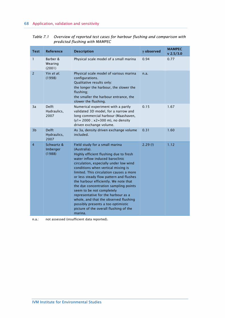
IVM Institute for Environmental Studies
68 Application, validation and sensitivity
Table 7.1 Overview of reported test cases for harbour flushing and comparison with predicted flushing with MAMPEC
Test Reference Description γ observed MAMPEC v 2.5/3.0
1 Barber & Wearing (2001)
Physical scale model of a small marina 0.94 0.77
2 Yin et al. (1998)
Physical scale model of various marina configurations. Qualitative results only:
the longer the harbour, the slower the flushing;
the smaller the harbour entrance, the slower the flushing.
n.a.
3a Delft Hydraulics, 2007
Numerical experiment with a partly validated 3D model, for a narrow and long commercial harbour (Maashaven, (y1= 2000 ; x2=300 m), no density driven exchange volume.
0.15 1.67
3b Delft Hydraulics, 2007
As 3a, density driven exchange volume included.
0.31 1.60
4 Schwartz & Imberger (1988)
Field study for a small marina (Australia).
Highly efficient flushing due to fresh water inflow induced baroclinic circulation, especially under low wind conditions when vertical mixing is limited. This circulation causes a more or less steady flow pattern and flushes the harbour efficiently. We note that the dye concentration sampling points seem to be not completely representative for the harbour as a whole, and that the observed flushing possibly presents a too optimistic picture of the overall flushing of the marina.
2.29 (!) 1.12
n.a.: not assessed (insufficient data reported).

IVM Institute for Environmental Studies
MAMPEC 3.0 HANDBOOK 69
7.3 Sensitivity
Like most steady state chemical fate models, the final exposure concentrations in MAMPEC are determined by the intensity of the emissions in combination with environmental conditions, such as e.g. the hydrodynamic exchange, sedimentation, and water characteristics, as well as compound-related properties, such as evapo-ration, (bio) degradation, and sorption to suspended particulate matter (SPM) and sediment. Discussions on the model sensitivity of MAMPEC can be found in Zipperle et al. (2011), Ohlauson et al. (2012), Gadd et al. (2011) and minutes and documentation of the Technical Meetings of competent authorities and member states of the former EU Biocide Products Directive (BPD) of the current Biocides Product Regulation (BPR). In Zipperle et al. (2011) a short summary of the sensitivity analysis of the model is provided and it is repeated here in a slightly modified form.
In simplified form the central mass balance equation and equilibrium statement (Equations. 4.14 and 6.1) can be stated as:
Emission + inflow - outflow - settling - volatilisation - decomposition = 0
The parameterisation of each of these processes determines the sensitivity of the model. The emission of antifouling compounds is dependent on paint-related factors (leaching rate, application factor and market share of product) and shipping charac-teristics (painted surface area, No. of ships, speed. Inflow and outflow of both dissolved compounds and substances bound to particulate matter are determined by the hydrodynamics (river flow, harbour geometry, tidal influence, wind speed), environmental characteristics (SPM, DOC), and compound properties (sorption to SPM, Koc). Input parameters important for the exchange in harbours are: the harbour entrance width, river current, density difference, and tidal prism. The process of settling is governed by environmental properties (SPM concentration, density, net sedimentation velocity, organic caerbon degradation) and compound related conditions (sorption and degradation). The volatilisation rate is a function of substance related parameters (Henry’s constant) and compartment specific variables (depth, temperature, gas-water mass transfer coefficients). The overall decomposition rate constant is a summation of the contributions of abiotic degradation (hydrolysis, photolysis) and biodegradation and are both substance and compartment specific. As an example, the photolysis rate constant is determined by both compound-related properties (spectral absorption, quantum yield) and factors determining the light penetration in the water column (e.g. average meteorology and water properties, DOC, SPM, Chlorophyll). For a number of parameters a temperature correction is in place (rate constants for biodegradation and hydrolysis, Henry’s constant). In the results screen of MAMPEC versions 3.0 and higher, a quick overview is presented of the relative contribution of these processes to the compound fluxes in the specific model runs (see section 6.6). In Zipperle et al. (2011) several exercises with MAMPEC 3.0 are presented (Table 7.2), demonstrating that the major processes affecting the final fate are: the hydrodynamic exchange, degradation processes, sorption properties and evaporation. For a number of different antifouling substances and ballast water related compounds in combination with different standard MAMPEC environments, the significance is indicated in table 7.2.
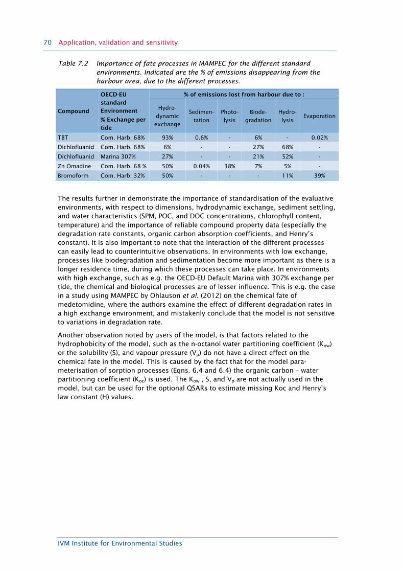
IVM Institute for Environmental Studies
70 Application, validation and sensitivity
Table 7.2 Importance of fate processes in MAMPEC for the different standard environments. Indicated are the % of emissions disappearing from the harbour area, due to the different processes.
Compound
OECD-EU standard Environment
% Exchange per tide
% of emissions lost from harbour due to :
Hydro-dynamic exchange
Sedimen-tation
Photo-lysis
Biode-gradation
Hydro-lysis
Evaporation
TBT Com. Harb. 68% 93% 0.6% - 6% - 0.02%
Dichlofluanid Com. Harb. 68% 6% - - 27% 68% -
Dichlofluanid Marina 307% 27% - - 21% 52% -
Zn Omadine Com. Harb. 68 % 50% 0.04% 38% 7% 5% -
Bromoform Com. Harb. 32% 50% - - - 11% 39%
The results further in demonstrate the importance of standardisation of the evaluative environments, with respect to dimensions, hydrodynamic exchange, sediment settling, and water characteristics (SPM, POC, and DOC concentrations, chlorophyll content, temperature) and the importance of reliable compound property data (especially the degradation rate constants, organic carbon absorption coefficients, and Henry’s constant). It is also important to note that the interaction of the different processes can easily lead to counterintuitive observations. In environments with low exchange, processes like biodegradation and sedimentation become more important as there is a longer residence time, during which these processes can take place. In environments with high exchange, such as e.g. the OECD-EU Default Marina with 307% exchange per tide, the chemical and biological processes are of lesser influence. This is e.g. the case in a study using MAMPEC by Ohlauson et al. (2012) on the chemical fate of medetomidine, where the authors examine the effect of different degradation rates in a high exchange environment, and mistakenly conclude that the model is not sensitive to variations in degradation rate.
Another observation noted by users of the model, is that factors related to the hydrophobicity of the model, such as the n-octanol water partitioning coefficient (Kow) or the solubility (S), and vapour pressure (Vp) do not have a direct effect on the chemical fate in the model. This is caused by the fact that for the model para-meterisation of sorption processes (Eqns. 6.4 and 6.4) the organic carbon – water partitioning coefficient (Koc) is used. The Kow , S, and Vp are not actually used in the model, but can be used for the optional QSARs to estimate missing Koc and Henry’s law constant (H) values.

IVM Institute for Environmental Studies
MAMPEC 3.0 HANDBOOK 71
8 Application for Ballastwater
The MAMPEC model is also being used for the exposure assessment of compounds emitted with discharges from ballast water treatment installations. Before 2011 the model was used on a voluntary basis by a number of applicants (summarised in Zipperle et al., 2011). On request of the GESAMP Ballast Water Working Group (BWGG) and IMO (UN International Maritime Organidasion) a special standardized version of MAMPEC for ballast water was created (MAMPEC BW v3.0) in 2011, with dedicated environment, compound and emissions scenarios. Currently the model is part of the evaluation methodology for basic and final approval by the MEPC (Marine Environmental Protection Committee) of IMO, based on the recommendations by GESAMP-BWWG (WG 34).
The environment screen of MAMPEC BW v3.0 for ballast water is identical to the environment screen for antifouling compounds (previous chapter). The most important difference is that a default GESAMP-BWWG Model Harbour has been included, with specifications and dimensions prescribed by the GESAMP-BWWG (STW3 4-6 April, 2011). This is one of the mandatory environment scenarios that new applicants need to use. Only a few standard environments relevant for ballast water have been added, such as the OECD-EU Shipping Lane and the OECD Commercial Harbour used for the risk assessment of antifoulants.
The GESAMP-BWWH Model harbour was derived from the OECD-EU Commercial Harbour, but with a lower hydrodynamic exchange (32% per tidal cycle), due to a lower mouth width of the harbour (1000 m compared to 2500 m in the OECD-EU Commercial Harbour) and a slightly increased pH (from 7.5 to 8.0). It is assumed to represent an average sized European harbour. The total area of the harbour is about 25% of the Port of Rotterdam. The dimensions were discussed during the stocktaking meetings of the GESAMP Ballast Water Working Group in 2009 (January and October) and 2011 (April) at IMO in London.
The database includes 18 relevant compounds, which regularly occurred in applica-tions for new ballast water treatment installations. Compound property data were derived from well-known official databases (TOXNET-HSDB, EpiSuite, GESAMPP databases) and reviewed by the GESAMP-BWWG (Meeting April 2011). For a number of properties, such as (bio)degradation, hydrolysis, and photolysis rates suitable data could not be found in official databases or reviewed literature. In such cases the worst-case assumption of no degradation was assumed. The 18 compounds are included as default entries in the database that cannot be changed by the user. Copies of the compounds can easily be edited and saved under a different user-defined name. Instructions of editing and entry of new data are provided in the quick manual or help files of the model. In future versions of MAMPEC-BW data for new compounds may be added. For version 3.01 an extension with 24 more compounds is expected.
Based on instructions from the GESAMP-BWWG and IMO an emission screen was made, allowing specification of the ballast water discharge rate (in m3/day) and the concentration of the target compound (in mg/L). Similarly as in the emission module for antifouling compounds the actual emission rates is calculated.

IVM Institute for Environmental Studies
72 Application for Ballastwater
The emission rate (g/day) is estimated according to:
3 3 ( / ) ( / ) ( / )BW BWTotal Emission g d Conc g m V m d= ⋅ (8.1)
in which:
Total Emission = amount of substance discharged in g/d
ConcBW = concentration in ballast water in g/m3 (equivalent to mg/L)
VBW = average volume of ballast water discharged per day in m3/d. For the default GESAMP-BWWG Model Harbour, with the settings recommended by the GESAMP Ballast Water Working Group and IMO, a default discharge volume of 100,000 m3/day is used, derived from a study for the harbour of Rotterdam in which the total ballast water discharges were estimated for this harbour (van Nieuw kerk, 2008). Discharge of this volume in a much smaller harbour (surface and volume of the model harbour are approximately 25% of that of the Port of Rotterdam) was considered as an adequate worst case situation for use in the risk assessment. The spatial allocation of emissions in the model harbour is similar as for the default commercial or estuarine harbour in MAMPEC (see Chapter 5); the emissions are distributed over the last row of cells (10 cells) along the back side of the harbour. Note that this also represents a worst case situation, compared to distribution along all sides of the harbour. As an example of the calculations the GESAMP BWWG 3 mg/L scenario was included.
The emission screen for ballastwater is only available in MAMPEC-BW 3.0. Further instructions on the use of the specific ballast water screens are explained in the manual and help files of the model.
In Zipperle et al. (2011) further guidance is given on the derivations of emission scenarios for contaminants in ballast water and the use of MAMPEC-BW. As discharges of ballastwater may have a high temporal and spatial variability, and some compounds may rapidly degrade, an evaluation was made to what extent MAMPEC-BW (a steady state model) was able to cope with this variability. Model runs with a dynamic model (DELWAQ) were compared with predictions obtained with MAMPEC. The average (temporal, spatial) exposure concentrations from ballast water treatment installations were well predicted by MAMPEC, but for time-varying and spatially dispersed discharge patterns substantial differences may occur, as expected. Cmax Concentrations of MAMPEC may underestimate the real maximum concentrations. Further recommen-dations how to approach maximum concentrations with short duration (< 2 hr) are presented in Zipperle et al. (2011)

IVM Institute for Environmental Studies
MAMPEC 3.0 HANDBOOK 73
References
Anonymous (2003). Daily hourly water levels at Turku in relation to theoretical mean sea level for year 2002. Finnish Institute of Marine Research.
Antonov, J.I., Locarnini, R.A., Boyer, T.P., Mishonov, A.V. & Garcia, H.E. (2006). World Ocean Atlas 2005, Volume 2: Salinity. Levitus, S. (Ed.), NOAA Atlas NESDIS 62. Washington, D.C.: U.S. Government Printing Office, 182 pp.
Arnold, W.R., Santore, R.C. & Cotsifas, J.S. (2005). Predicting copper toxicity in estuarine and marine waters using the biotic ligand model. Marine Pollution Bulletin, 50, 1634–1640.
Baart, A.C. (2003). Mam-Pec, application at low exchange conditions. Report Z3662, WL| Delft Hydraulics, Delft.
Baart, A., Boon, J. & van Hattum, B. (2008). User manual – quick guide MAMPEC version 2.0. Deltares|Delft Hydraulics, Delft – Institute for Environmental Studies (IVM), Vrije Universiteit Amsterdam, The Netherlands.
Barber, R.W. & Wearing, M.J. (2001). A mathematical model for estimating the pollution exchange coefficient of small tidal embayments. Proceedings 1st Int. Conf. on Water Resources Management, University of Thessaloniki, Greece, September 2001, pp. 233-240.
Bayer, A.G. (2002). Preventol A 4-S – Summary of toxicity and ecotoxicity. Product information sheet dichlofluanid, edition 2002-07-02. Bayer AG, Leverkusen Berg EA (1995). European Coatings Journal, 7, 534.
Bockting, G.J.M., van de Plassche, E.J., Struijs, J. & Canton, J.H. (1993). Soil-water partition coefficients for organic compounds. RIVM Report no. 679101013, p. 46.
Boethling, R., Fenner, K., Howard, P., Klečka, G., Madsen, T., Snape, J. R. & Whelan, M. J. (2009). Environmental Persistence of Organic Pollutants: Guidance for Development and Review of POP Risk Profiles. Integrated Environmental Assessment and Management, 5, 539–556.
Boethling, R.S & Mackay, D. (Eds) (2000). Handbook of property estimation methods for chemicals – Environmental Health Sciences. New York (USA): Lewis Publishers.
Boon, J., Baart, A., Markus, A. & van Hattum, B. (2008). Antifoulant model to predict environmental concentrations (MAMPEC V2.0) - Technical background additional features of MAMPEC version 2.0. Report Z-3820. Deltares|Delft Hydraulics, Delft - Institute for Environmental Studies, Vrije Universiteit Amsterdam, The Netherlands.
Boxall, A.B.A., Comber, S.D., Conrad, A.U., Howcroft, J. & Zaman, N. (2000). Inputs, monitoring and fate modelling of antifouling biocides in UK estuaries. Marine Pollution Bulletin, 40, 898-905
Burns, L.A. (2005). Exposure Analysis Modelling System. EXAMS. User manual and system documentation. US EPA 600/R-00/081.
CEPE (2003). Provision of biocide leaching rate data for anti-fouling products: a discussion document from the Anti-Fouling Working Group of CEPE. Included as Annex-II in the OECD-EU Emission Scenario Document for antifoulants: van der Plassche and van der Aa (2004).
CEPE-AFWG (1998) Classes of biocidal antifouling paint commercially available in the European Union, CEPE, Brussels
Delft Hydraulics (1989). Lozingen in Havens, Modellen voor de verspreiding van water-0 en bodemverontreinigende stoffen in havens als instrument bij vergunningverlening, (in Dutch). Research Report T262_1 (two volumes), October 1989.

IVM Institute for Environmental Studies
74 References
Delft Hydraulics (2007). Beoordeling koelwaterlozing AVR Brielselaan, Report Z4337 (in Dutch).
Delft Hydraulics research report S 61, June 1977
Delft Hydraulics, 2003. Light penetration in the water column. report WL 2003001/Z3379.
Delft Hydraulics, 2005. Delft3D-WAQ. User manual
Di Toro, D.M., Allen, H., Bergman, H., Meyer, J., Paquin, P. & Santore, R. (2001). A Biotic Ligand Model of the Acute Toxicity of Metals: I. Technical Basis. Environmental Toxicology and Chemistry, 20,2383-2396.
DOE (1994). Chapter 5, Physical and thermodynamic data. In Dickson, A.G. & Goyet, C. (Eds) (1994). Handbook of methods for the analysis of the various parameters of the carbon dioxide system in sea water. Report ORNL/CDIAC-74. U. S. Department of Energy, http://cdiac.esd.ornl.gov/ftp/cdiac74/chapter5.pdf
Donat, J.R., Lao, K.A. & Bruland, K.W. (1994). Speciation of dissolved copper and nickel in south San Fransisco bay: a multi-method approach. Analytica Chimica Acta, 284, 547–571.
Drebs, A., Nordlund, A., Karlsson, P., Helminen, J. & Rissanen, P. (2002). Climatological Statistics of Finland 1971–2000. Finnish Meteorological Institute. Helsinki.
Early, E.P., Brandon, L., Swope, L., Barbeau, K., Bundy, R., McDonald, J.A. & Rivera-Duarte, I. (2013). Life cycle contributions of copper from vessel painting and maintenance activities. Biofouling, 30, 51–68.
ECB (1997). EUSES - The European union system for the evaluation of substances. Joint Research Centre European Commission Environment Institute, European Chemicals Bureau, Ispra (1997).
Eisma, D. & Kalf, J. (1987). Distribution, organic content and particle size of suspended matter in the North Sea. Netherlands Journal of Sea Research, 21(4), 265-285.
Eleveld, M.A., Pasterkamp, R., van der Woerd, H.J. & Pietrzak, J.D. (2008). Remotely sensed seasonality in the spatial distribution of sea-surface suspended particulate matter in the southern North Sea. Estuarine. Coastal and Shelf Science, 80, 103–113.
EU Workshop (2006). Harmonisation of leaching rate determinations for antifouling products under the biocidal products directive. Report of Workshop of technical experts competent authorities BPD (98/8/EC, 2007) and stakeholders held in Ispra (Italy), 12 December 2006. Available from: http://ihcp.jrc.ec.europa.eu/our_activities/public-health/risk_assessment_of_Biocides/doc/ESD/ ESD_PT/PT_21/PT_21_Leaching_Workshop.pdf.
Evans, R.D. (1994). Empirical evidence for the importance of sediment resuspension in lakes. Hydrobiologia, 284, 5-12.
Eysink, W.D. (2004). SILTHAR version 4.2, a mathematical program for the computation of siltation in harbour basins. User manual WINDOWS-PC program. Delft Hydraulics, August, 2004, report 8.6520.
Farrington, J.W. (1991). Biogeochemical processes governing exposure and uptake of organic pollutant compounds in aquatic organisms. Environmental Health Perspect, 90, 75-84.
Finnie, A.A. (2006). Improved estimates of environmental copper release rates from antifouling products. Biofouling, 22, 279–291.
Fischer, H.B., List, J.E., Koh, C.R., Imberger, J. & Brooks, N.H. (1979). Mixing in inland and coastal waters. New York: Academic Press.
Gadd, J., Depree, C. & Hickey, C. (2011). Relevance to New Zealand of the OECD Emission Scenario Document for Antifouling Products: Phase 2 Report. Report no. ERM10201;

IVM Institute for Environmental Studies
MAMPEC 3.0 HANDBOOK 75
HAM 2011-005. NIWA report for the Environmental Protection Authority (EPA), Wellington, New Zealand. pp. 108
Gadd, J & Cameron, M. (2012). Antifouling biocides in marinas: Measurement of copper concentrations and comparison to model predictions for eight Auckland sites. Prepared by NIWA for Auckland Council. Auckland Council – technical report TR2012/033. National Institute of Water & Atmospheric Research Ltd., Hamilton, New Zealand.
Gallegos, C.L. (2000). Factors contributing to water-column light attenuation. SAV Technical Synthesis II, Chapter 4. In Batiuk, R.A., Bergstrom, P., Kemp, M., Koch, E., Murray, L., Stevenson, J.C., Bartleson, R., Carter, V., Rybicki, N., Landwehr, J., Gallegos, C., Karrh, L., Naylor, M., Wilcox, D., Moore, K. & Ailstock, S. (2000). Chesapeake Bay submersed aquatic vegetation water quality and habitat-based requirements and restoration targets: a second technical synthesis. U.S. EPA Chesapeake Bay Program. Annapolis, MD, USA.
Gerritsen, H. Goede, E.D., Genseberger, M. & Uittenbogaard, R.E. (2003). Validation document Delft3D-FLOW, Report nr. X0289, WL| Delft Hydraulics, Delft.
Gobas, F.A.P.C. & Maclean, L.G. (2003). Sediment-water distribution of organic contaminants in aquatic ecosystems: the role of organic carbon mineralization. Environmental Science & Technology, 37, 735–741.
Gordon, A.S., Dyer, B.J., Kango, R.A. & Donat, J.R. (1996). Copper ligands isolated from estuarine water by immobilized metal affinity chromatography:temporal variability and partial charac-terization. Marine Chemistry, 53, 163–172.
van de Graaf, J. & Reinalda, R. (1977) Horizontal exchange in distorted scale models. Report nr. S61, WL|Delft Hydraulics, Delft (in Dutch)
van Hattum, B., Baart, A.C., Boon, J.G., Steen, R.J.C.A. & Ariese, F. (1999). Computer model to generate predicted environmental concentrations (PECs) for antifouling products in the marine environment. IVM report (E-99/15). Institute for Environmental Studies, VU University Amsterdam, 68 pp.
Hervouet, J.M. (2000). Hydrological Processes, 13, 2209.
Sabljic, A. & Güsten, H. (1995). QSARs for soil sorption. In Hermens, J.L.M. (Ed.), Overview of structure-activity relationships for environmental endpoints. Report prepared within the framework of the project “QSAR for Prediction of Fate and Effects of Chemicals in the Environment”, an international project of the Environmental Technologies RTD Programme (DG XII/D-1) of the European Commission under contract number EV5V-CT92-0211.
Holtrop, J. (1977) A statistical analysis of performance test results. International Shipbuilding Progress, 24(270), 23-28.
Howard, P.H. & Meylan, W.M. (1997). Prediction of physical properties, transport, and degradation for environmental fate and exposure assessments. In Chen, F. & Schüürmann, G. (Eds), Quantitative structure-activity relationships in environmental sciences – VII. Pensacola (Fl, USA): SETAC Press.
Isnard, P. & Lambert, S. (1989). Aqueous solubility and n-octanol/water partition coefficient correlations. Chemosphere, 18, 1837-1853.
ISO (2010) Paints and varnishes – Modelling of biocide release rate from antifouling paints by mass-balance calculation ISO nr 10890:2010. International Organization for Standardization, Geneva (Switzerland). Available from: http://www.iso.org
Karickhoff, S.W. (1984). Organic pollutant sorption in aquatic systems. Journal of Hydraulic Engineering, 110, 707-735.
Karman, C.C., Kramer, K.J.M. & Jak, R.G. (1998). Bioavailability of copper in the marine environment -an ecological risk assessment for releases from copper based anti-fouling paints. Report No. CR97 - 032 R 98/382. . Institute of Environmental Sciences, Energy

IVM Institute for Environmental Studies
76 References
Research and Process Innovation (TNO-MEP), Department of Ecological Risk Studies, Den Helder (Netherlands).
Kersten, M., Dicke, M., Kriews, M., Naumann, K., Scmidt, D., Schulz, M., Schwikowski, M. & Steiger, M. (1988). Distribution and fate of heavy metals in the North Sea.
Kiil, S., Dam-Johansen, K., Weinell, C.E., Pedersen, M.S. & Codolar, S.A. (2003). Estimation of polishing and leaching behaviour of antifouling paints using mathematical modelling: a literature review. Biofouling, 19, 3743.
Lamoree, M.H., Swart, C.P., van der Horst, A. & van Hattum, B. (2002). Determination of diuron and the antifouling paint biocide Irgarol 1051 in Dutch marinas and coastal waters. Journal of Chromatography A, 970, 183–190.
Lesser, G.R., Roelvink, J.A. & van Kester, J.A.T.M. (2004). Development and validation of a three-dimensional morphological model. Coastal Engineering, 51, 883–915.
Lyman, W.J., Reehl, W.F. & Rosenblatt, D.H. (1990). Handbook of chemical property estima-tion methods: environmental behaviour of organic compounds. American Chemical Society (ACS), Washington (DC).
Mackay, D., Shiu, W.Y. & Ma, K.C. (1997). Illustrated handbook of physical-chemical properties of environmental fate for organic chemicals. Springer-Verlag, Berlin/Heidelberg.
McClimans, T.A., Pietrzak, J.D., Huess, V. et al. (2000). A comparison of laboratory and numerical simulations of the ocean circulation in the Skagerrak. Continental Shelf Research, 20, 941–974.
Meylan, W. & Howard, P. (1999). User’s guide for EPIWIN. EPI Suite – Estimation Programs Interface for Microsoft Windows. Syracuse Research Corporation, North Syracuse (NY).
Mill, T. (2000). Photoreactions in surface waters. In Boethling, R.S & Mackay, D. (Eds), Handbook of property estimation methods for chemicals – Environmental Health Sciences. New York (USA): Lewis Publishers, pp. 355-282.
Miller, L.A. & Bruland, K.W. (1997). Competitive equilibration techniques for determining transition metal speciation in natural waters: Evaluation using model data. Analytica Chimica Acta, 343, 161–181.
Morris, A.W. & Riley, J.P. (1966). The bromide/chlorinity and sulphate/chlorinity ratio in sea water. Deep-Sea Research, 13, 699–705.
Neely, W.B. & Blau, G.E. (1985). Environmental exposure from chemicals, Volume I, pp. 186–187. Boca Raton, Florida: CRC Press, Inc.
Nendza, N. & Hermens, J. (1995). Properties of chemicals and estimation methodologies. In van Leeuwen, C.J. & Hermens, J.L.M. (Eds), Risk assessment of chemicals: an introduction. Dordrecht, Boston, London: Kluwer Academic Publishers.
Omae, I. (2003). Organotin antifouling paints and their alternatives. Applied Organometallic Chemistry, 17, 81.
Ohlauson, C., Eriksson, K.M. & Blanck, H. (2012). Short-term effects of medetomidine on photosynthesis and protein synthesis in periphyton, epipsammon and plankton communities in relation to predicted environmental concentrations. Biofouling 28, 491–9.
van Pagee, J.A., Glas, P.C.G, Markus, A.A. & Postma, L. (1988). Mathematical modeling as a tool for assessment of North Sea pollution. In Salomons, W., Bayne, B.L., Duursma, E.K. & Förstner, U. (Eds), Pollution of the North Sea: an assessment. Berlin: Springer-Verlag.
Riley, J.P. & Tongudai, M. (1967). The major cation / chlorinity ratios in sea water. Chemical Geology, 2, 263–269.
Riley, J.P. (1965). The occurrence of anomalously high fluoride concentrations in the North Atlantic. Deep-Sea Research, 12, 219–220.

IVM Institute for Environmental Studies
MAMPEC 3.0 HANDBOOK 77
Ruiz, C.E. & Gerald, T. (2001). RECOVERY version 2, a mathematical model to predict the temporal response of surface water to contaminated sediments. Report No. ERDC/EL TR-01-3. U. S. Army Corps of Engineers, Research and Development Center, Vicksburg, MS (USA). Available at: http://el.erdc.usace.army.mil/products.cfm?Topic=model&Type=watqual
Sabljic, A. & Güsten, H. (1995). QSARs for soil sorption. In Hermens, J.L.M. (Ed.), Overview of structure-activity relationships for environmental endpoints. Report prepared within the framework of the project “QSAR for Prediction of Fate and Effects of Chemicals in the Environment”, an international project of the Environmental Technologies RTD Programme (DG XII/D-1) of the European Commission under contract number EV5V-CT92-0211.
Santore, R.C., Di Toro, D.M., Paquin, P.R., Allen, H.E. & Meyer, J.S. (2001). A biotic ligand model of the acute toxicity of metals: II. Application to acute copper toxicity in freshwater fish and daphnia. Environmental Toxicology and Chemistry, 20(10), 2397–2402.
Schwartz & Imberger (1988). Flushing behaviour of a coastal marina. Proc. 21st Int. Coastal Engineering Conf., Spain, ED 439.
Steen, R.J.C.A., Jacobsen, J., Ariese, F., van Hattum, A.G.M. & Jacobson, A. (2004). Monitoring of the marine antifoulant 4,5-dichlor-2-n-octyl-4-isothiazolin-3-one (DCOI) in a Danish harbor. Chemosphere, 57, 513–521.
Stewart, C. (2003). Antifouling co-biocides in New Zealand coastal waters. Report prepared for Ministry for the Environment, Wellington. New Zealand
Stewart, C. (2006). Antifouling co-biocides in New Zealand coastal waters: 2006 resurvey. Prepared for Ministry for the Environment, Wellington, New Zealand.
Stronkhorst, J. & van Hattum, B. (2003). Contaminants of concern in Dutch marine Harbor Sediments. Archives of Environmental Contamination and Toxicology, 45, 306–316.
TGD (1996). Technical guidance document in support of commission directive 93/67/EEC on risk assessment for new notified substances and commission regulation (EC) No 1488/94 on risk assessment for existing substances. Office for Official Publications of the European Communities, Luxembourg.
TGD (2003). Technical Guidance Document on Risk Assessment in Support of Commission Directive 93/67/EEC on Risk Assessment for New Notified Substances and Commission Regulation (EC) No 1488/94 on Risk Assessment for Existing Substances and Directive 98/8/EC of the European Parliament and the Council Concerning the placing of biocidal products on the market. Part II. European Commission Joint Research Centre, EUR 20418 EN/2, © European Communities 2003. Office for official Publications of the European Communities, Luxembourg. Available at: http://echa.europa.eu/documents/10162/16960216/tgdpart2_2ed_en.pdf
Thomas, K.V., Blake, S.J. & Waldock, M.J. (2000). Antifouling paint booster biocide contamination in UK marine sediments. Marine Pollution Bulletin, 40,739–745.
Thomas, K.V., Raymond, K., Chadwick, J. & Waldock, M. (1999). The effects of short-term changes in environmental parameters on the release of biocides from antifouling coatings: cuprous oxide and tributyltin. Applied Organometallic Chemistry, 13,453–460.
Thomas, K.V. (2001). The environmental fate and behaviour of antifouling paint booster biocides: A review. Biofouling 17, 73–86.
Tilastoja Suomen Ilmastosta (2002). 1971 – 2000 (Climatological statistics of Finland 1971 – 2000); Ilmatieteen Laitos Meteorologiska Institutet (Finnish Meteorological Institute), 2002:1

IVM Institute for Environmental Studies
78 References
Tipping, E. (1994). WHAM – A chemical equilibrium model and computer code for waters, sediments and soils incorporating a discrete site/electrostatic model of ion binding by humic substance. Computational Geosciences, 20, 973–1023.
Turley, P.A., Fenn, R.J. & Ritter, J.C. (2000). Pyrithiones as antifoulants: environmental chemistry and preliminary risk assessment. Bio-fouling, 15, 175–182.
UNESCO (1966) Second report of the Joint Panel on Oceanographic Tables and Standards. UNESCO Technical Papers in Marine Science No. 4.
van der Plassche, E. & van der Aa, E. (2004). Harmonisation of environmental emission scenarios: an emission scenario document for antifouling products in OECD countries (ESD-PT21), Royal Haskoning, Nijmegen (NL). Available from http://ihcp.jrc.ec.europa.eu/ and MAMPEC support site
van Hattum, B. & Baart, A.C. (2002). User manual – quick guide Mam-Pec version 1.4. IVM Report. (E-02/03). Institute for Environmental Studies, Vrije Universiteit Amsterdam, 20 pp.
van Hattum, B., Baart, A.C. & Boon, J.G. (2002). Computer model to generate predicted environmental concentrations (PECs) for antifouling products in the marine environment - 2nd edition accompanying the release of Mam-Pec version 1.4. IVM Report. (E-02/04). Institute for Environmental Studies, Vrije Universiteit Amsterdam, 80 pp.
van Hattum, B. & Baart, A. (2001). TBT – a compound currently in the lime light. In Gandrass, J. & Salomons, W. (Eds), Dredged material in the Port of Rotterdam – interface between Rhine Catchment Area and North Sea (pp. 277-288). GKSS Research Centre, Geesthacht (Germany).
van Hattum, B., Baart, A. & Boon, J. (2006). Emission estimation and chemical fate modelling of antifoulants. In Konstantinou, I.K. (Ed.), Antifouling Paint Biocides. Handbook of Environmental Chemistry Vol. 5/O (pp. 101-120). Berlin (Germany): Springer Verlag.
van Niekerk. H. (2008). Ballast water quantities Port of Rotterdam. Ballast water intake and discharge. February 2008. Report No. 9T2104. Port of Rotterdam. Rotterdam (Netherlands)
Williamson, R.B., Wilcock, R.J., van Dam, L.F., Lee, D.J. & Schriner, R. (1995). The characteristics and fate of copper-based antifouling paint residues in the marine environment around Auckland 1995. ARC Technical Report TP 33. Auckland Regional Council, 58 pp., New Zealand.
WL, Delft Hydraulics, 2003. Light penetration in the water column. Report WL 2003001/Z3379, Delft Hydraulics (Deltares), Delft.
WL, Delft Hydraulics, 2005. Delft3D-Flow. User manual, Delft Hydraulics (Deltares), Delft.
WL, Delft Hydraulics, 1978. Wind Effect on the Distribution of Velocity and Temperature in stratified enclosed systems, Report R898 II. Delft Hydraulics (Deltares), Delft.
Yin, J., Falconer, R., Pipilis, K. & Stamou, A. (1998). Flow characteristics and flushing processes in marinas and coastal embayments. 1st Int. Conf Maritime Engineering and Ports, 1998. pp. 87-98.
Zepp, R.G & Cline, D.M. (1977). Rates of direct photolysis in aquatic environment. Environmental Science & Technology, 11, 359–366.
Zipperle, A., van Gils, J., van Hattum, B. & Heise, S. (2011). Guidance document for a harmonized Emission Scenario Document (ESD) on Ballast Water discharge. Report 36301205 prepared for Umwetlbundesamt, Dessau. BIS-beratungszentrum für integriertes Sedimentmanagement, Technishe Hochschshule Hamburg-Harburg, Hamburg, Germany (available via MAMPEC support site)

IVM Institute for Environmental Studies
MAMPEC 3.0 HANDBOOK 79
Annex A Version history
Since the first release of MAMPEC in 1999 (v1.2), various new releases have been issued in 2002 (v1.4), 2006 (v1.6), 2008 (v2.0 and 2.5), and 2011 (v.30 and MAMPEC-BW v3.0). Based on requests from users, competent authorities and member states new elements and functions were added to the new versions. Detailed information about the version history can be found in the release notes of the different versions (available on support site). In most cases updates did not affect the calculation of PECs. Due to bug fixes in the exchange formulations and default settings mostly small changes occurred between some default scenarios of the OECD-EU Workgroup (ESD-PT21; van der Plassche et al., 2004) in versions v2.5 and higher compared to older versions (v 1.4- v2.0). The differences are described in the release notes of v2.5 (available at support site). PECs calculated in v3.0 and v2.5 are identical for the Commercial Harbour and Marina scenarios; due to changes in settings of the Open Sea and Shipping Lane scenarios (sediment and water characteristics; emission data) PECs in v3.0 are different from PECs in v2.5 for these scenarios. This is described in more detail in the release notes of version 3.0
Version 3.0
In this new version (v3.0) further improvements and bug fixes are included, as well as several important new features:
• Compatibility to current and expected upgrades of the Windows XP/VISTA/7 OS • Conversion of program code from Visual Basic v6.0 to .NET framework and C# in to
meet current standards and software requirements • Inclusion of standard EU and OECD emission scenarios for non-service life
emissions • Improved user interface and workflow, database management, as well as handling
of input and output screens • Multiple run option allowing to run multiple scenario combinations and to facilitate
sensitivity analysis • Analysis of main compound fluxes and significance and contribution of different
chemical fate processes • Plot of predicted environmental concentrations downstream of harbour • Copper speciation: new option to export results and create an input file for the
widely used BLM model , to facilitate further analysis of the copper speciation • Improved import and export options of database settings and predicted results.
Settings from previous versions (v2.0, v2.5) can easily be imported. • Improved entry of degradation rate data. Values can be entered both as half-life or
as rate constants • Multi-lingual support: in addition to English and Japanese (since v2.5) new
translations in v3.0 are: Chinese and Spanish. • Bug fixes: input settings environment for Open Sea and Shipping Lane scenarios

IVM Institute for Environmental Studies
80
MAMPEC-BW v3.0 (July 2011)
With support of for the International Maritime Organization (IMO) and the ballast water working group (BWWG) of the Joint Group of Experts on the Scientific Aspects of Marine Environmental Protection (GESAMP) a special version for ballast water (MAMPECBW) was developed for the exposure assessment of chemicals in ballast water according to guidelines based on the IMO Ballastwater Convention of 2004. Special adaptations compared to the standard version of MAMPEC v.30 include:
• Inclusion of evaluation scenarios, as recommended by GESAMP-BWWG for environment (GESAMP-BWWG Model Harbour) and emissions (Default Emission GESAMP-BWWG Model Harbour)
• Default values of many chemical property data for 18 compounds, as recommended by GESAMP-BWWG (Workshop April, 2011).
Version 2.5 (December 2008)
• multilanguage framework with Japanese as first foreign language implementation • improved sediment module with parameters for degradation of sediment organic
matter • improved hydrodynamic exchange calculation (bug fix in exchange mechanism)
V2.0 (February 2008)
Inclusion of some new additional features and updated chemical process formulations (photolysis):
• inclusion of wind-driven hydrodynamic exchange; • extension of environmental scenarios (open harbour) • correction zero-tidal exchange formulations (for e.f. freshwater applications) • export compounds / environments & emissions (to new dbase format) • import compounds / environments & emissions (from new dbase format) • advanced photolysis module • calculation of PECs in the area outside the harbour (for new runs) • additional fields in the database to accommodate the new
functionalities; • automatic update of previous database to accommodate the new features
V1.6 (2006)
• Inclusion of standard OECD-EU scenarios (ESD-PT21; van der Plassche et al. 2004)
v1.4 (2002)
• Bug fix to accommodate country settings of Win 2000/XP • Extended help files • Extension of default scenarios • Additional module for sediment processes – extension on request of regulators
Version v.1.2 (1999)
The first proto-type version of the MAMPEC model