ist-4-027756 winner ii d1.1.1 v1.1 winner ii … - interim report.pdf · winner ii interim channel...
TRANSCRIPT

WINNER II D1.1.1 V1.1
Page 1 (153)
IST-4-027756 WINNER II
D1.1.1 V1.1
WINNER II interim channel models
Contractual Date of Delivery to the CEC: 30/11/2006
Actual Date of Delivery to the CEC: 30/11/2006 (updated 09/02/2007)
Author(s): Pekka Kyösti, Juha Meinilä, Lassi Hentilä, Xiongwen Zhao, Tommi Jämsä, Christian Schneider, Milan Narandzić, Marko Milojević, Aihua Hong, Juha Ylitalo, Veli-Matti Holappa, Mikko Alatossava, Robert Bultitude, Yvo deJong, Terhi Rautiainen
Participant(s): EBITT, TUI, UOULU, CU/CRC, NOKIA
Workpackage: WP1 Channel Model
Estimated person months: 62
Security: PU
Nature: R
Version: 1.1
Total number of pages: 153
Abstract: This deliverable describes WINNER II interim channel models for link and system level simulations. Both generic and clustered delay line models are defined for selected propagation scenarios.
Keyword list: Channel modelling, propagation scenario, wideband, channel sounder, cluster, delay domain, angle domain, polarisation, measurements, delay spread, angle spread, arrival, departure, MIMO
Disclaimer: The channel models described in this deliverable are based on a literature survey and measurements performed during this project. The authors are not responsible for any loss, damage or expenses caused by potential errors or inaccuracies in the models or in the deliverable.

WINNER II D1.1.1 V1.1
Page 2 (153)
Executive Summary This deliverable presents WINNER II interim channel models for link level and system level simulations of short range and wide area wireless communication systems. The models have been evolved from the WINNER channel models described in WINNER I deliverable D5.4. The covered propagation scenarios are indoor small office, large indoor hall, indoor-to-outdoor, urban micro-cell, bad urban micro-cell, outdoor-to-indoor, stationary feeder, suburban macro-cell, urban macro-cell, rural macro-cell, and rural moving networks.
The generic WINNER II interim channel model follows a geometric-based stochastic channel modelling approach, which allows creating of virtually unlimited double directional radio channel model. The channel models are antenna independent, i.e., different antenna configurations and different element patterns can be inserted. The channel parameters are determined stochastically, based on statistical distributions extracted from channel measurement. The distributions are defined for, e.g., delay spread, delay values, angle spread, shadow fading, and cross-polarisation ratio. For each channel snapshot – segment – the large scale and small scale parameters are calculated from the distributions. Channel realisations are generated with geometrical principle by summing contributions of rays with specific small scale parameters like delay, power, angle-of-arrival and angle-of-departure. Different scenarios are modelled by using the same approach, but different parameters. The parameter tables for each scenario are included in this deliverable.
Clustered delay line (CDL) models with fixed large-scale and small-scale parameters have also been created for calibration and comparison of different simulations. The parameters of the CDL models are based on expectation values of the generic models.
Several measurement campaigns provide the background for the parameterisation of the propagation scenarios for both LOS and NLOS conditions. These measurements were conducted by five partners with different devices. The developed models are based on both literature and extensive measurement campaigns that have been carried out within the WINNER I and WINNER II projects.
The novel features of the WINNER models are its parameterization, the consideration of elevation in indoor scenarios, auto-correlation modelling of large-scale parameters (including cross-correlation), smooth time evolution of channel parameters, and scenario-dependent polarization modelling. The models are scalable from a single SISO or MIMO link to a multi-link MIMO scenario including polarization among other radio channel dimensions.
WINNER II interim channel models can be used in link level and system level performance evaluation of wireless systems, as well as comparison of different algorithms, technologies and products. The models can be applied not only to WINNER II system, but also any other wireless system operating in 2 – 6 GHz frequency range with maximum 100 MHz RF bandwidth. The model supports also multi-antenna technologies, polarization, multi-user, multi-cell, and multi-hop networks.

WINNER II D1.1.1 V1.1
Page 3 (153)
Authors
Partner Name Phone / Fax / e-mail
EBITT Pekka Kyösti Phone: +358 40 344 2000
Fax: +358 8 551 4344
e-mail: [email protected]
EBITT Juha Meinilä Phone: +358 40 344 2000
Fax: +
e-mail: [email protected]
EBITT Tommi Jämsä Phone: +358 40 344 2000
Fax: +358 8 551 4344
e-mail: [email protected]
EBITT Xiongwen Zhao Phone: +358 40 344 2000
Fax: +358 9 2561014
e-mail: [email protected]
EBITT Lassi Hentilä Phone: +358 40 344 2000
Fax: +358 8 551 4344
e-mail: [email protected]
UOULU Mikko Alatossava Phone: +358 8 814 7638
Fax: +358 8 553 2845
e-mail: [email protected]
UOULU Veli-Matti Holappa Phone: +358 8 814 2890
Fax: +358 8 553 2845
e-mail: [email protected]
WINNER II D1.1.1 V1.1
Page 4 (153)
TUI Milan Narandžić Phone: + 49 3677 69 3722
Fax: + 49 3677 69 1113
e-mail: [email protected]
TUI Aihua Hong Phone: + 49 3677 69 1157
Fax: + 49 3677 69 1113
e-mail: [email protected]
TUI Marko Milojević Phone: + 49 3677 69 2673
Fax: + 49 3677 69 1195
e-mail: [email protected]
TUI Christian Schneider Phone: + 49 3677 69 1157
Fax: + 49 3677 69 1113
e-mail: [email protected]
TUI Gerd Sommerkorn Phone: + 49 3677 69 1115
Fax: + 49 3677 69 1113
e-mail: [email protected]
CRC Robert Bultitude Phone: 1-613-98-2775
Fax: 1-613-990-7987
e-mail: [email protected]
CRC Yvo deJong Phone: 1-603-990-9235
Fax: 1-613-990-6339
e-mail: [email protected]
NOK Terhi Rautiainen Phone: +358 50 4837218
Fax: + 358 7180 36857
e-mail: [email protected]
WINNER II D1.1.1 V1.1
Page 5 (153)
Table of Contents
Part I ............................................. ..................................................................... 9
1. Introduction ....................................... .......................................................... 9
2. Definitions ........................................ ......................................................... 11
2.1 Terminology .............................................................................................................................. 11 2.2 List of Symbols ......................................................................................................................... 14 2.3 Propagation Scenarios ............................................................................................................... 16
2.3.1 A1 – Indoor small office ................................................................................................... 17 2.3.2 A2 – Indoor to outdoor...................................................................................................... 17 2.3.3 B1 – Urban micro-cell....................................................................................................... 18 2.3.4 B2 – Bad Urban micro-cell ............................................................................................... 18 2.3.5 B3 – Indoor hotspot........................................................................................................... 18 2.3.6 B4 – Outdoor to indoor ..................................................................................................... 18 2.3.7 B5 – Stationary Feeder...................................................................................................... 18 2.3.8 C1 – Suburban macro-cell................................................................................................. 20 2.3.9 C2 – Urban macro-cell ...................................................................................................... 20 2.3.10 C3 – Bad urban macro-cell ............................................................................................... 21 2.3.11 D1 – Rural macro-cell ....................................................................................................... 21 2.3.12 D2 – Moving networks...................................................................................................... 21
2.4 Measurement Tools ................................................................................................................... 21 2.4.1 Propsound (EBITT, UOULU, Nokia) ............................................................................... 21 2.4.2 TUI sounder ...................................................................................................................... 23 2.4.3 CRC sounder ..................................................................................................................... 24
3. Channel Modelling Approach ......................... ......................................... 26
3.1 Stochastic models ...................................................................................................................... 27 3.2 Network layout .......................................................................................................................... 27
3.2.1 Correlations between large scale parameters .................................................................... 27 3.3 Concept of channel segments and time evolution ..................................................................... 31 3.4 Reduced complexity models...................................................................................................... 33
3.4.1 Cluster Delay Line models for mobile and portable scenarios.......................................... 34 3.4.2 Cluster Delay Line models fixed feeder links ................................................................... 34 3.4.3 Cluster delay line models for fixed multi-hop scenarios................................................... 34
4. Channel Models and Parameters...................... ....................................... 36
4.1 Applicability .............................................................................................................................. 36 4.1.1 Environment dependence .................................................................................................. 36 4.1.2 System dependence ........................................................................................................... 36
4.2 Generation of Channel Coefficients .......................................................................................... 36 4.2.1 Generation of bad urban channels (B2, C3) ...................................................................... 40
4.3 Path-loss models........................................................................................................................ 41 4.4 Parameter tables for generic models.......................................................................................... 44
4.4.1 Reference output values .................................................................................................... 47 4.5 Transitions between propagation conditions ............................................................................. 48 4.6 CDL Models .............................................................................................................................. 49

WINNER II D1.1.1 V1.1
Page 6 (153)
4.7 Comparison of Phase I and Phase II models.............................................................................. 49
5. Channel Model Usage................................ ............................................... 53
5.1 System level description............................................................................................................ 53 5.1.1 Coordinate system............................................................................................................. 53 5.1.2 Multi-cell simulations ....................................................................................................... 54 5.1.3 Multihop and relaying....................................................................................................... 56 5.1.4 Interference ....................................................................................................................... 57
5.2 Space-time concept in simulations ............................................................................................ 58 5.2.1 Time sampling and interpolation....................................................................................... 58
5.3 Radio-environment settings....................................................................................................... 58 5.3.1 Scenario transitions ........................................................................................................... 58 5.3.2 LOS\NLOS transitions ...................................................................................................... 58
5.4 Bandwidth/Frequency dependence............................................................................................ 58 5.4.1 Frequency sampling .......................................................................................................... 58 5.4.2 Bandwidth down scaling................................................................................................... 58 5.4.3 FDD modeling................................................................................................................... 59
Part II ............................................ ................................................................... 60
6. Measurement and Analysis Results ................... ..................................... 60
6.1 A1 – Indoor small office............................................................................................................ 60 6.1.1 Path-loss and shadow fading............................................................................................. 60 6.1.2 Angular Spreads at BS and MS......................................................................................... 62
6.2 A2 – Indoor to outdoor .............................................................................................................. 64 6.2.1 Path-loss and shadow fading............................................................................................. 64 6.2.2 DS and maximum excess delay distribution ..................................................................... 69 6.2.3 Azimuth AS at BS and MS ............................................................................................... 70 6.2.4 Cross-polarisation ratio (XPR).......................................................................................... 71 6.2.5 Power Delay Profile .......................................................................................................... 73 6.2.6 Proportionality factor of the delay .................................................................................... 73 6.2.7 Power Angular Spectrum and main DoA offset................................................................ 74 6.2.8 Number of clusters ............................................................................................................ 74 6.2.9 Time evolution of clusters................................................................................................. 75 6.2.10 Per cluster shadowing ....................................................................................................... 76 6.2.11 Ricean K-factor ................................................................................................................. 76
6.3 B1 – Urban micro-cell ............................................................................................................... 80 6.3.1 Path-loss and shadow fading............................................................................................. 80 6.3.2 Rms delay spread results by CU/CRC .............................................................................. 82 6.3.3 LOS probability................................................................................................................. 84
6.4 B2 – Bad urban micro-cell......................................................................................................... 85 6.5 B3 – Indoor hotspot ................................................................................................................... 85 6.6 B4 – Outdoor to indoor.............................................................................................................. 85
6.6.1 Path-loss and shadow fading............................................................................................. 85 6.6.2 RMS and maximum excess delay distribution .................................................................. 88 6.6.3 Azimuth AS at BS and MS ............................................................................................... 91 6.6.4 Elevation AS at BS ........................................................................................................... 93 6.6.5 Cross-polarisation ratio (XPR).......................................................................................... 94 6.6.6 Power Delay Profile .......................................................................................................... 94

WINNER II D1.1.1 V1.1
Page 7 (153)
6.6.7 Proportionality factors, delay and angular ........................................................................ 95 6.6.8 Main DoA and DoD offset ................................................................................................ 98 6.6.9 Ricean K-factor ............................................................................................................... 100 6.6.10 Cross-Correlations .......................................................................................................... 102 6.6.11 Distributions.................................................................................................................... 103 6.6.12 Outdoor-to-indoor results by CU/CRC ........................................................................... 104 6.6.13 Combined results............................................................................................................. 106
6.7 B5 – Stationary Feeder ............................................................................................................ 106 6.7.1 B5a– Fixed Stationary Feeder: Roof-top to Roof-top (LOS) .......................................... 106 6.7.2 B5c – Fixed Stationary Feeder: Below Roof-top to Street Level.................................... 107 6.7.3 B5f – Fixed Stationary Feeder: Roof-top to Roof-top (NLOS)....................................... 108
6.8 C1 – Suburban macro-cell ....................................................................................................... 109 6.8.1 Path loss and shadow fading ........................................................................................... 110 6.8.2 DS and maximum excess delay distribution ................................................................... 111 6.8.3 Azimuth AS at BS and MS ............................................................................................. 112
6.9 C2 – Urban macro-cell ............................................................................................................ 112 6.9.1 Path-loss and shadow fading........................................................................................... 112 6.9.2 DS and maximum excess delay distribution ................................................................... 114 6.9.3 Azimuth AS at BS and MS ............................................................................................. 116
6.10 C3 – Bad urban macro-cell ...................................................................................................... 117 6.11 D1 – Rural macro-cell ............................................................................................................. 118
6.11.1 Path-loss and shadow fading........................................................................................... 118 6.12 D2 – Moving networks ............................................................................................................ 120
6.12.1 Path-loss and shadow fading........................................................................................... 121 6.12.2 RMS-delay spread and maximum excess delay distributions ......................................... 121 6.12.3 Azimuth AS at BS and MS ............................................................................................. 122 6.12.4 Cross-polarisation ratio (XPR)........................................................................................ 123 6.12.5 Power Delay Profile ........................................................................................................ 124 6.12.6 Distribution of path delays .............................................................................................. 124 6.12.7 Delay proportionality factor............................................................................................ 125 6.12.8 Power Angular Spectrum and main DoA offset.............................................................. 125 6.12.9 Number of clusters .......................................................................................................... 125 6.12.10 Per-cluster shadowing.......................................................................................... 126 6.12.11 Ricean K-factor.................................................................................................... 126 6.12.12 Literature research ............................................................................................... 126 6.12.13 Interpretation of the results .................................................................................. 127
6.13 Peer-to-peer channel models ................................................................................................... 127
7. Parameter Tables for CDL Models.................... ..................................... 127
7.1 A1 – Indoor small office.......................................................................................................... 127 7.2 A2 – Indoor to outdoor ............................................................................................................ 129 7.3 B1 – Urban micro-cell ............................................................................................................. 129 7.4 B2 – Bad Urban micro-cell...................................................................................................... 131 7.5 B3 – Indoor hotspot ................................................................................................................. 131 7.6 B4 – Outdoor to indoor............................................................................................................ 133 7.7 C1 – Urban macro-cell ............................................................................................................ 133 7.8 C2 – Urban macro-cell ............................................................................................................ 135 7.9 C3 – Bad urban macro-cell ...................................................................................................... 135 7.10 D1 – Rural macro-cell ............................................................................................................. 136

WINNER II D1.1.1 V1.1
Page 8 (153)
7.10.1 D2a – Moving networks.................................................................................................. 137 7.11 Fixed feeder links - Scenario B5 ............................................................................................. 138
7.11.1 Scenario B5a ................................................................................................................... 138 7.11.2 Scenario B5b................................................................................................................... 138 7.11.3 Scenario B5c ................................................................................................................... 141 7.11.4 Scenario B5f.................................................................................................................... 141
8. Reference Implementation Interfaces ................ ................................... 143
8.1.1 Example of input parameters .......................................................................................... 143 8.1.2 Example of output parameters ........................................................................................ 148
9. References......................................... ...................................................... 149

WINNER II D1.1.1 V1.1
Page 9 (153)
Part I
1. Introduction The goal of WINNER is to develop a single ubiquitous radio access system adaptable to a comprehensive range of mobile communication scenarios from short range to wide area. This will be based on a single radio access technology with enhanced capabilities compared to existing systems or their evolutions. WINNER II is a continuation of the WINNER I project, which developed the overall system concept. WINNER II will develop and optimise this concept towards a detailed system definition. [WINNERII]
The radio interface will support the challenging requirements of systems beyond 3G. It will be scalable in terms of carrier bandwidth and carrier frequency range. The system will support a wide range of radio environments providing a significant improvement in performance and Quality of Service. The radio interface will optimise the use of spectral resources, e.g. through the exploitation of actual channel conditions and multiple antenna technology. New networking topologies (e.g. relaying) will support cost-effective deployments. Support of advanced resource management and handover will ease the deployment of the WINNER system enabling seamless service provision and global roaming. [WINNERII]
It has been widely understood that radio propagation has a significant impact on the performance of wireless communication systems. The impact on future broadband systems is even more important. Because of the major influence on the system performance and complexity, radio channel models and simulations have to be more versatile and accurate than in earlier systems.
WINNER I work package 5 (WP5) focused on wideband MIMO channel modelling at 5 GHz frequency range. Totally six partners were involved in WP5 during 2004 – 2005, namely Elektrobit, Helsinki University of Technology, Nokia, Royal Institute of Technology (KTH) in Stockholm, Swiss Federal Institute of Technology (ETH) in Zurich, and Technical University of Ilmenau. In the beginning of Phase I, existing channel models were explored to find out channel models for the initial use in the WINNER I project. Based on the literature survey, two standardised models were selected, namely 3GPP/3GPP2 Spatial Channel Model (SCM) and IEEE 802.11n. The former is used in outdoor simulations and the latter in indoor simulations. Because the bandwidth of the SCM model is on 5 MHz, wideband extension (100 MHz) for it was developed in WINNER I. However, in spite of the modification, the initial models were not adequate for the advanced WINNER I simulations. Therefore, new measurement-based models were developed in WINNER I. WINNER I generic model was created in Phase I. It allows creating of virtually unlimited double directional radio channel model. The generic model is ray-based multi-link model that is antenna independent, scalable and capable of modelling channels for MIMO connections. Extracted statistical distributions and channel parameters from measurement data of new propagation scenarios can be fitted to the generic model. WINNER I interim channel models delivered during Phase I are based on those channel measurements performed at 2 and 5 GHz bands during the project.
The SCM, SCME, and WINNER I channel models were implemented in Matlab, and are available via WINNER web site.
In the WINNER II project, a set of multidimensional channel models are developed. They cover wide scope of propagation scenarios and environments, including indoor-to-outdoor, outdoor-to-indoor, bad urban micro-cell, bad urban macro-cell, feeder link BS-FRS, and moving networks BS-MRS, MRS-MS. They are based on more generic channel modelling approach, which means the possibility to vary number of antennas, the antenna configurations, geometry and the beam antenna pattern without changing the basic propagation model. This method enables the use of the same channel data in different link level and system level simulations and it is well suited for evaluation of adaptive radio links, equalisation techniques, coding, modulation, and other transceiver techniques.
This deliverable describes the interim version of WINNER II channel models. The models are based on WINNER I models (D5.4). New scenarios and new features (time evolution of large scale parameters, intra cluster delay spread, and far cluster option) are included. CDL models are based on expectation values of stochastic models large scale parameters.
This deliverable is divided into two major parts. This first part (Sections 1 - 5) is the main part and defines the channel model structure and parameters. This second part (Sections 6 - 8) contains more detailed information about channel measurements, analysis, and the channel model implementation. The Sections 1 - 8 cover the following topics. Section 1 introduces this deliverable. Section 2 defines the

WINNER II D1.1.1 V1.1
Page 10 (153)
terminology, symbols, propagation scenarios, and used measurement tools. Section 3 defines the channel modelling approach. Section 4 explains the generation of channel coefficients and describes path loss models as well as parameters for generic models. Section 4 includes also comparison of Phase I and Phase II models. Section 5 discusses how the channel models are used in system level (multi-link) simulations, sampling, transition scenarios, bandwidth/frequency dependence of the models. Section 6 reports the channel measurement and analysis results. Parameter tables for CDL models can be found from Section 7. Reference implementation interfaces are described in Section 8. Reference list is in Section 9.

WINNER II D1.1.1 V1.1
Page 11 (153)
2. Definitions
2.1 Terminology
3GPP 3rd Generation Partnership Project
3GPP2 3rd Generation Partnership Project 2
ACF Auto-Correlation Function
ADC Analog-to-Digital Converter
AN Antenna Array
AoA Angle of Arrival
AoD Angle of Departure
APP A Posteriori Probability
APS Angle Power Spectrum
AS Azimuth Spread
ASA Azimuth Spread at Arrival
ASD Azimuth Spread at Departure
AWGN Additive White Gaussian Noise
B3G Beyond 3G
BER Bit Error Rate
BRAN Broadband Radio Access Networks
BS Base Station
BW Bandwidth
C/I Carrier to Interference ratio
CDF Cumulative Distribution Function
CDL Clustered Delay Line
CG Concept Group
CIR Channel Impulse Response
CRC Canadian Research Center
CW Continuous Wave
D3SF Double-Directional Delay-Spread Function
DoA Direction of Arrival
DoD Direction of Departure
DS/DES Delay Spread
EBIT Elektrobit Ltd
EBITT Elektrobit Testing Ltd
ECDF Experimentally determined cumulative probability distribution function
ESA Elevation Spread at Arrival
ESD Elevation Spread at Departure
ESPRIT Estimation of Signal Parameters via Rotational Invariance Techniques
ETHZ Eidgenössische Technische Hochschule Zürich (Swiss Federal Institute of Technology Zurich)
ETSI European Telecommunications Standards Institute
FDD Frequency Division Duplex
FIR Finite Impulse Response
FRS Fixed Relay Station
FS Fixed Station
GPS Global Positioning System
HIPERLAN High Performance Local Area Network
HUT Helsinki University of Technology (TKK)

WINNER II D1.1.1 V1.1
Page 12 (153)
IR Impulse Response
ISIS Initialization and Search Improved SAGE
KF K Factor
KTH Kungliga Tekniska Högskolan (Royal Institute of Technology in Stockholm)
LA Local Area
LNS Log-Normal Shadowing
LOS Line-of-Sight
LS Large Scale
MA Metropolitan Area
MCSSS Multi-Carrier Spread Spectrum Signal
METRA Multi-Element Transmit and Receive Antennas (European IST project)
MIMO Multiple-Input Multiple-Output
MPC Multi-Path Component
MRS Mobile Relay Station
MS Mobile Station
MUSIC Multiple Signal Classification
NACM No Auto-Correlation Mode
NL Network Layout
NLOS Non Line-of-Sight
NOK Nokia
OFDM Orthogonal Frequency-Division Multiplexing
OLOS Obstructed Line-of-Sight
PAS Power Azimuth Spectrum
PD3S Power Double-Directional Delay-Spectrum
PDF Probability Distribution Function
PDP Power-Delay Profile
PL Path Loss
PN Pseudo Noise
RIMAX Maximum likelihood parameter estimation framework for joint superresolution estimation of both specular and dense multipath components
RF Radio Frequency
RMS Root Mean Square
RT Roof-top
RX Receiver
SAGE Space-Alternating Generalized Expectation-maximization
SCM Spatial Channel Model
SCME Spatial Channel Model Extended
SF/SHF Shadow Fading
SIMO Single-Input Multiple-Output
SISO Single-Input Single-Output
SoS Sum of Sinusoids
STD Standard deviation
SW Software
TDD Time Division Duplex
TDL Tapped Delay-Line
TUI Technische Universität Ilmenau
TX Transmitter
UOULU University of Oulu
WA Wide Area

WINNER II D1.1.1 V1.1
Page 13 (153)
WINNER Wireless World Initiative New Radio
WPx Work Package x of WINNER project
XPR Cross-Polarisation power Ratio
XPRH Horizontal Polarisation XPR
XPRV Vertical Polarisation XPR

WINNER II D1.1.1 V1.1
Page 14 (153)
2.2 List of Symbols
∆(•) Change in parameter value
(•)T Transpose
(•)H Hermitian transpose
(•)* Complex conjugate
log10(•) base 10 logarithm
cos(•) Cosine of the argument
sin(•) Sine of the argument
A Pairing matrix
C Correlation matrix
Ftx Tx antenna array response matrix
Frx Rx antenna array response matrix
H MIMO channel transfer matrix
N Normal distribution
U Uniform Distribution
ϕ AoA
φ AoD
τ Delay
σt RMS delay spread
σϕ RMS angle spread of AoA
σφ RMS angle spread of AoD
cAoA cluster-wise RMS angle spread of AoA
cAoD cluster-wise RMS angle spread of AoA
σSF Shadow fading standard deviation
σ2 Variance
ζ Per cluster shadowing standard deviation
λ Wavelength
λ0 Wave number
κvh Vertical-to-horizontal XPR
κhv Horizontal-to-vertical XPR
υ Doppler frequency
α Complex gain of a propagation path
c Speed of light
fc Central frequency
hbs BS antenna height
hbs’ Effective BS antenna height
hms MS antenna height
hms’ Effective MS antenna height
KR Ricean K-factor
n Index to cluster
P Power
rϕ AoA distribution proportionality factor
rφ AoD distribution proportionality factor

WINNER II D1.1.1 V1.1
Page 15 (153)
rb Break point distance
rt Delay distribution proportionality factor
s Index to Tx antenna element
t Time
u Index to Rx antenna element

WINNER II D1.1.1 V1.1
Page 16 (153)
2.3 Propagation Scenarios
The propagation scenarios modelled in WINNER are shown in Table 2-1. The propagation scenarios are explained in more detail in the following paragraphs. Mapping of scenarios to Concept Groups is shown in the table Table 2-1 in column CG.
Table 2-1. Propagation scenarios specified in WINNER. Scenarios modelled in Phase II are emphasized with bold font.
Scenario Definition LOS/ NLOS
Mob. km/h
Frequency (GHz)
CG Note
A1 In building
Indoor small office / residential
LOS/ NLOS
0–5 2 - 6 LA
A2
Indoor to outdoor
NLOS 0–5 2 - 6 LA AP inside UT outside. Outdoor environment urban
B1 Hotspot
Typical urban micro-cell
LOS
NLOS
0–70 2 - 6 LA,
MA
Typical distance ranges. Actual ranges depend on frequency and antenna heights
B2
Bad Urban micro-cell
LOS/ NLOS
0–70 2 - 6 MA Same as B1 + long delays
B3 Hotspot
Large indoor hall
LOS 0–5 2 - 6 LA
B4
Outdoor to indoor. -Outdoor typical urban. -Indoor A1
NLOS
0–5 2 - 6 MA B1 or C2 to the wall/window.
B5a
Hotspot Metropol
LOS stat. feeder, rooftop to rooftop
LOS 0 2 - 6 MA Same channel model for hot spot and metropol.
B5b Hotspot Metropol
LOS stat. feeder, street-level to street-level
LOS 0 2 - 6 MA Typical distance ranges. Actual ranges depend on frequency and antenna heights
B5c Hotspot Metropol
LOS stat. feeder, below- rooftop to street-level
LOS 0 2 - 6 MA Typical distance range. Actual range depends on frequency and antenna heights
B5d
Hotspot Metropol
NLOS stat. feeder, above rooftop to street-level
NLOS
0 2 - 6 MA Extended C2
B5f
Feeder link BS -> FRS. Approximately RT to RT level.
LOS/ OLOS/NLOS
0 2 - 6 WA Desired link: LOS or OLOS, Interfering links: LOS/(OLOS) /NLOS FRS -> MS = B1*

WINNER II D1.1.1 V1.1
Page 17 (153)
Table 2-1 (continued).
2.3.1 A1 – Indoor small office The scenario A1, has been modelled in D5.4. The layout of the scenario is shown in Figure 5-2.
8-element antenna array8-element antenna array
Rooms: 10 x 10 x 3 m
Corridors: 5 x 100 x 3 m
Figure 2-2. Layout of the A1 indoor scenario.
2.3.2 A2 – Indoor to outdoor In indoor-to-outdoor scenario (Figure 5-9) the MS antenna height is assumed to be at 1 – 2 m, and BS antenna height at 2 – 2.5 m + floor height. The corresponding outdoor and indoor environments are B1 an A1, respectively. It is assumed that the floors 1 to 3 are used in simulations, floor 1 meaning the ground floor.
Scenario Definition LOS/ NLOS
Mob.
km/h
Frequency (GHz)
CG Note
C1
Metropol
Suburban LOS/ NLOS
0–120 2 - 6 WA
C2
Metropol
Typical urban
macro-cell
NLOS 0–120 2 - 6 MA
WA
C3 Bad Urban macro-cell
LOS/ NLOS
0–70 2 - 6 - Same as C2 + long delays
D1 Rural
Rural macro-cell LOS/ NLOS
0–200 2 - 6 WA
a) Moving networks:
BS – MRS, rural
LOS 0 –350
2 - 6 WA Very large Doppler variability.
D2
b) Moving networks:
MRS – MS, rural
LOS /
OLOS/
NLOS
0 – 5 2 - 6 LA Not finished yet!

WINNER II D1.1.1 V1.1
Page 18 (153)
MS
BS
LOS/NLOS
Figure 2-9: Indoor to outdoor scenario.
2.3.3 B1 – Urban micro-cell In urban micro-cell scenarios the height of both the antenna at the BS and that at the MS is assumed to be well below the tops of surrounding buildings. Both antennas are assumed to be outdoors in an area where streets are laid out in a Manhattan-like grid. The streets in the coverage area are classified as “the main street”, where there is LOS from all locations to the BS, with the possible exception of cases in which LOS is temporarily blocked by traffic (e.g. trucks and busses) on the street. Streets that intersect the main street are referred to as perpendicular streets, and those that run parallel to it are referred to as parallel streets. This scenario is defined for both LOS and NLOS cases. Cell shapes are defined by the surrounding buildings, and energy reaches NLOS streets as a result of propagation around corners, through buildings, and between them.
2.3.4 B2 – Bad Urban micro-cell Bad urban micro-cell scenarios are identical in layout to Urban Micro-cell scenarios, as described above. However, propagation characteristics are such that multipath energy from distant objects can be received at some locations. This energy can be clustered or distinct, has significant power (up to within a few dB of the earliest received energy), and exhibits long excess delays. Such situations typically occur when there are clear radio paths across open areas, such as large squares, parks or bodies of water.
2.3.5 B3 – Indoor hotspot Scenario B3 represents the propagation conditions pertinent to operation in a typical indoor hotspot, with wide, but non-ubiquitous coverage and low mobility (0-5 km/h). Traffic of high density would be expected in such scenarios, as for example, in conference halls, factories, train stations and airports, where the indoor environment is characterised by larger open spaces, where ranges between a BS and a MS or between two MS can be significant. Typical dimensions of such areas could range from 20 m × 20 m up to more than 100m in length and width and up to 20 m in height. Both LOS and NLOS propagation conditions could exist.
2.3.6 B4 – Outdoor to indoor Outdoor-to-indoor in urban macrocell (C4) is identical with B4 because the antenna heights are irrelevant as explained in Chapter 7.6. In outdoor-to-indoor scenario the MS antenna height is assumed to be at 1 – 2 m (plus the floor height), and the BS antenna height below roof-top, at 5 - 15 m depending on the height of surrounding buildings (typically over four floors high). Outdoor environment is metropolitan area B1, typical urban microcell where the user density is typically high, and thus the requirements for system throughput and spectral efficiency are high. The corresponding indoor environment is A1, typical indoor small office. It is assumed that the floors 1 to 3 are used in simulations, floor 1 meaning the ground floor.
2.3.7 B5 – Stationary Feeder Fixed feeder links scenario is described in [WIN1D54] and defined as propagation scenario B5. This scenario has also been partly modelled in [WIN1D54]. In B5, both terminals are fixed. Based on this, the scenario was divided in four categories or sub-scenarios in [WIN1D54. These are B5a (LOS stationary feeder: rooftop to rooftop), B5b (LOS stationary feeder: street level to street level), B5c (LOS stationary feeder: below rooftop to street level) and B5d (NLOS stationary feeder: rooftop to street level). Height of street level terminal antenna is assumed to be 3-5 meters. To cover the needs of CG WA one modified sub-scenario is needed in phase 2, scenario B5f: LOS/NLOS stationary feeder: rooftop-to-below/above rooftop. All the sub-scenarios will be described below.

WINNER II D1.1.1 V1.1
Page 19 (153)
In stationary scenarios, the Doppler shifts of the rays are not a function of the AoAs. Instead, they are obtained from the movement of the scatterers. In B5 we let one scatterer per cluster be in motion while the others are stationary. In [TPE02] a theoretical model is built where the change of phase of scattered waves between time t and t+∆t is given by
( ) ( )ppc t
c
f αγπ coscos4 ∆ (2.1)
where pα is the angle between the direction of scatterer movement and pγ the direction orthogonal to
the reflecting surface and the reflection angle. By proper selection of these angles different Doppler spectrums may be achieved. For B5d also an additional term in the path-loss model has to be included.
The feeder scenarios are specified here in connection of the micro-cellular environment. Actually the feeders can be used also in the macro-cellular cases. In this document it is assumed that the useful macro-cellular feeder link, C5, is identical with the feeder model B5c.
2.3.7.1 B5a
The signal in B5a can be assumed to consist of a strong LOS signal and single bounce reflection. Also far away reflections can occur. The connection is almost like in free space, so that the path-loss does not depend noticeably on the antenna heights. For this scenario fixed angle spread, delay spread and XPR values are applied. Directive antennas are very effective in reducing the delay spread and other multi-path impacts as explained in [PT00]. However, the model is applicable for omni-directional antennas for up to 300 meters in distance. By using directive antennas the range can be extended approximately to 8 km.
A static (non-fading) channel component is added to the impulse response. We select this parameter to be 10 dB. The power-delay profile (of all paths except the direct) is set as exponential, based on the results in [OBL+02] and [SCK05]. The shadow fading is Gaussian with mean zero and standard deviation of 3.4 dB based on [PT00]. B5a sub-scenario was specified and modelled in [WIN1D54]. The same channel model is used also in Phase II.
2.3.7.2 B5b
In B5b it is assumed that both the transmitter and receiver have many scatterers in their close vicinity similar as theorized in [Sva02]. In addition there can also be long echoes from the ends of the street. There is a LoS ray between the transmitter and receiver and when this path is strong, the contribution from all the scatters is small. However, beyond the breakpoint distance the scatterers start to play an important role.
In papers e.g. [Bal02], [SBA+02] the results for different carrier frequencies are very similar. Therefore, in B5b model the frequency is disregarded. The principle adopted for the WINNER phase 1 model allows for various correlations between different parameters such as angle-spread, shadow-fading and delay-spread. In this case, dependency between path loss and delay-spread [MKA02] is applied. This dependence is handled by selecting one of three different CDL models given in [WIN1D54]. Based on the delay-spread formula in [MAS02] we select the delay spread to be 30 ns when the path loss is less than 85 dB, 110 ns when the path loss is between 85 dB and 110 dB, and finally 380 ns when the path loss is greater than 110 dB. With these settings the delay-spread used here is a factor 40%-156% of the delay-spread formula of [MAS02] for path losses up to 137 dB. We call these path-loss intervals range1, range2 and range3 and different clustered-delay line models will be provided for the three cases.
In terms of path loss, the break point distance calculated as
( )( )λ
0b0bb 4
hhhhr
−−=
(2.2)
becomes important leading to so called two slope -model. The power delay profile (of all paths except the direct) is set as exponential, based on the results in [SMI+00]. A per-path shadow fading of 3 dB is used to obtain some variation in the impulse responses. A static (non-fading) channel component is added to the impulse response. Based on [FDS+94] we select this parameter to be 10 in range1, 2 in range2, and 1 in range3. Also K-factor changes according to range. B5b sub-scenario was specified and modelled in [WIN1D54]. The same channel model is used also in Phase II.

WINNER II D1.1.1 V1.1
Page 20 (153)
2.3.7.3 B5c and B5d
B5c and B5d can be considered as LOS of B1 and NLOS of C2 respectively. Only support for Doppler spectrum of stationary cases has to be introduced. B5c is probably the most important Feeder link scenario, because it will be used in urban micro-cell relay scenario. B5c is almost identical to the B1 micro-cellular LOS scenario. The only difference in environment is the assumed antenna height of the mobile/relay. Same channel model will cover both of the cases, except the difference in Doppler spectrum (mobility). Feeder link ends are stationary and the Doppler frequency results from motion of the environment. In B5c some clusters represent vehicles with speed of ~50 km/h and the rest of the clusters represent stationary objects like walls and building corners.
Actually B5d seems less useful for a Feeder link scenario. Therefore it is not discussed here further.
2.3.7.4 B5f
The sub-scenario is shown in the figure below.
Feeder-link B5f
Master-station
MS
Relay
Relay to MS: B1
Feeder-link B5f
Master-station
MS
Relay
Relay to MS: B1
Interfering Feeder-link
MS
Relay
Relay to MS: B1
BS
Relay
Desired Feeder-link
a b c
Figure 2-1 B5f scenario for three cases: a) NLOS (OLOS) b) LOS c) Combined interference case.
B5f scenario consists of the cases with relay antennas some meters over the roof-top or some meters below the roof-top. Key point is, if the link is LOS or NLOS: It is possible to create LOS links with the antennas below roof-tops. As well it is possible to implement NLOS links with antennas above the average roof-top level. Our approach is that the desired BS to FRS links can be planned to be LOS or OLOS, or at least “good” links. It is assumed that the interfering links from undesired BS to FRS can be LOS or NLOS. (Although in practice this can be also affected by careful planning.) It should be pointed out that the link FRS to MS is covered by the model B1. Interference to undesired feeder link may occur.
In B5f it is assumed that the relay station is shadowed due to some obstacle. The proposed model is based on literature and formed from the B5a LOS fixed relay model by attenuating artificially its direct component by 15 dB in average and summing to it a normally distributed random decibel number with standard deviation 8 dB. The path loss formula is based on the references [ZEA99] and [GEA03]. The other model parameters are the same as in B5a. The model B5f can also be understood as NLOS part of the model B5a.
2.3.8 C1 – Suburban macro-cell In suburban macro-cells base stations are located well above the rooftops to allow wide area coverage, and mobile stations are outdoors at street level. Buildings are typically low residential detached houses with one or two floors, or blocks of flats with a few floors. Occasional open areas such as parks or playgrounds between the houses make the environment rather open. Streets do not form urban-like regular strict grid structure. Vegetation is modest.
2.3.9 C2 – Urban macro-cell In typical urban macro-cell mobile station is located outdoors at street level and fixed base station clearly above surrounding building heights. As for propagation conditions, non- or obstructed line-of-sight is a common case, since street level is often reached by a single diffraction over the rooftop. The building blocks can form either a regular Manhattan type of grid, or have more irregular locations. Typical building heights in urban environments are over four floors. Buildings height and density in typical urban macro-cell are mostly homogenous.

WINNER II D1.1.1 V1.1
Page 21 (153)
2.3.10 C3 – Bad urban macro-cell Bad urban environment describes cities with buildings with distinctly inhomogeneous building heights or densities, and results to a clearly dispersive propagation environment in delay and angular domain. The inhomogeneties in city structure can be e.g. due to large water areas separating the built-up areas, or the high-rise skyscrapers in otherwise typical urban environment. Increased delay and angular dispersion can also be caused by mountainous surrounding the city. Base station is typically located above the average rooftop level, but within its coverage range there can also be several high-rise buildings exceeding the base station height. From modelling point of view this differs from typical urban macro-cell by an additional far scatterer cluster.
2.3.11 D1 – Rural macro-cell Propagation scenario D1 represents radio propagation in large areas (radii up to 10 km) with low building density. The height of the AP antenna is typically in the range from 20 to 70 m, which is much higher than the average building height. Consequently, LOS conditions can be expected to exist in most of the coverage area. In case the UE is located inside a building or vehicle, an additional penetration loss is experienced which can possibly be modelled as a (frequency-dependent) constant value. The AP antenna location is fixed in this propagation scenario, and the UE antenna velocity is in the range from 0 to 200 km/h.
In WINNER Phase I, measurements were conducted in a flat rural environment near Oulu in Finland, at both 2.45 and 5.25 GHz, and with an AP antenna height of 18 - 25 m. A channel model derived from these measurements is available and has been reported in [WIND54]. The channel model from Phase I for propagation scenario D1 is generalised for the frequency range 2 – 6 GHz and different BS and MS antenna heights.
2.3.12 D2 – Moving networks Propagation scenario D2 (“Rural Moving Network”) represents radio propagation in environments where both the AP and the UE are moving, possibly at very high speed, in a rural area. A typical example of this scenario occurs in carriages of high-speed trains where wireless coverage is provided by so-called moving relay stations (MRSs) which can be mounted, for example, to the ceiling. Note that the link between the fixed network and the moving network (train) is typically a LOS wireless link whose propagation characteristics are represented by propagation scenario D1.
2.4 Measurement Tools
Five different radio channel measurement systems have been used in the propagation measurements during Phase I and II. Main characteristics of the channel sounders used in Phase II are summarised in this section.
2.4.1 Propsound (EBITT, UOULU, Nokia) Propsound™ multi-dimensional radio channel sounder is a product of Elektrobit, Finland [PSound]. Propsound has been designed so that it suits very well to realistic radio channel measurements both in time- and spatial-domains. It is based on the spread spectrum sounding method in the delay domain. The other dimensions like polarizations, FDD frequencies or spatial dimensions over antenna arrays are covered using an advanced time-domain switching. Together with optional super-resolution techniques (SAGE algorithm) this allows accurate measurements of SISO, SIMO, MIMO, geolocation and multi-user propagation channels. Some key features of Propsound are presented in Table 2-2.
Table 2-2 PropsoundTM characteristics
Propsound Property Range of values
RF bands 1.7 - 2.1, 2.0 - 2.7, 3.2 - 4.0, 5.1 - 5.9 GHz
Sustained measurement rate Up to 30.000 CIR/s (code length: 255 chips)
Maximum cycle (snapshot) rate 1500 Hz
Chip frequency up to 100 Mchips/s
Useable code lengths 31 - 4095 chips (M-sequences)

WINNER II D1.1.1 V1.1
Page 22 (153)
Number of measurement channels up to 8448
Measurement modes SISO, SIMO, MIMO
Receiver noise figure better than 3 dB
Baseband sampling rate up to 2 GSamples/s
Spurious IR free dynamic range: 35 dB
Transmitter output up to 26 dBm (400 mW), adjustable in 2 dB steps
Control Windows notebook PC via Ethernet
Post processing MATLAB package
Synchronisation rubidium clock with stability of 10 e-11
Table 2-3 PropsoundTM terminals.
Trasmitter with a trolley.
Receiver with a trolley.
Table 2-4 PropsoundTM antennas.
Name ODA_5G25 PLA_5G25 UCA_5G25
Array structure omnidirectional array rectancular array uniform circular array
Polarization dual (+/- 45) dual (+/- 45) vertical
Center frequency [GHz]
5.25 5.25 5.25
Number of elements 50 (25 dual) 32 (16 dual) 8
Element type patch patch monopole
Schematic plot

WINNER II D1.1.1 V1.1
Page 23 (153)
Name ODA_5G25 PLA_5G25 UCA_5G25
Picture
2.4.2 TUI sounder
The channel sounder RUSK TUI-FAU used in TU Ilmenau MIMO measurements is designed by Medav, Germany [Medav]. The RUSK is a real-time radio channel impulse response measurement system that supports multiple transmit and receive antenna element configurations.
The RUSK MIMO channel sounder measures the channel response matrix between all transmitting and receiving antenna elements sequentially by switching between different (Tx,Rx) antenna element pairs. This means that sounder uses only one physical transmitter and receiver channel, what reduces the sensitivity to channel imbalance. A switched antenna approach offers the simple way to change number of antenna elements in array. Additionally, since antennas are not transmitting at the same time there is no need for separation of transmitted signals at the receiver side. To accomplish synchronous switching, rubidium reference oscillators are used both at transmitter and receiver. Timing and switching frame synchronization is established during an initial synchronization process prior to measurement data recording and must be maintained over the complete measurement time.
For channel excitation RUSK uses multi-carrier spread spectrum signal (MCSSS) with almost rectangular shape in frequency domain. That allows the precise concentration of the signal energy into the band of interest. In this way multiple bands (e.g. separated up- and down-link bands in FDD) are supported by setting some spectral magnitudes to zero. Table 2-5 summarizes the key features of the RUSK TUI-FAU channel sounder.
Table 2-5 Key features of the Medav RUSK TUI-FAU channel sounder.
RUSK TUI-FAU Sounder Property Range of values
RF bands 5…6 GHz
Max. meas. data storage rate (2x)*160 Mbyte/s
Test signal Multi Carrier Spread Spectrum Signal (MCSSS)
Sequence length
(defines maximum excess delay)
256 – 8192 spectral lines, depending on IR length
Number of measurement channels up to 65536 (216 )
Measurement modes SISO, SIMO, MIMO
Sampling frequency 640 MHz at Tx and Rx
Spurious free IR dynamic range: 48 dB
Transmitter output up to 33 dBm (2 W),
Propagation delay resolution 4.17 ns (1/bandwidth)

WINNER II D1.1.1 V1.1
Page 24 (153)
Impulse response length 0.8 µs – 25.6 µs
RF sensitivity -88 dBm
Control Windows PC
Post processing MATLAB package
Synchronisation rubidium clock with stability of 10-10
* rate is doubled with additional disk storage. Second storage enables shorter time gap between Tx-Rx sub-channels.
Overview of measurement-relevant technical data for antenna arrays used in TU-Ilmenau campaigns is given in Table 2-6.
Table 2-6 Overview of TU-Ilmenau antenna arrays.
Name PULA8
(PULA8@10W) UCA16 PUCPA24 SPUCPA4x24
Vendor IRK Dresden TU Ilmenau IRK Dresden IRK Dresden
Array structure uniform linear array uniform circular
array uniform circular
array stacked uniform
circular array
Polarization dual (vertical+
horizontal) vertical
dual (vertical+ horizontal)
dual (vertical+ horizontal)
Center frequency
[GHz] 5.2 5.2 5.2 5.2
Bandwidth [MHz] 120 120 120 120
Max. Power [dBm] 27 (40) 27 25 24
Number of elements 8 16 24 96
Element type patch disk cone patch Patch
Dimensioning
element spacing
0.4943 λ diameter 10.85 cm
diameter 19.5 cm
diameter 19.5 cm
ring spacing 0.4943 λ
Element orientation
Picture
Monopol antenna that is mounted on ICE roof was manufactured by Huber+Suhner, type: SWA 0859 – 360/4/0/DFRX30. Disc-conical antenna used for ICE SISO measurements is designed by Kurt Blau (TU Ilmenau) for 5.2 GHz range.
2.4.3 CRC sounder The sounder used for the CRC measurements is the fourth generation of a PN sounder design that was first implemented with 20 MHz bandwidth at CRC in 1981. Its construction is bread-board style, with semi-rigid cables connecting various commercially-available modules, such as phase-locked oscillators, power splitters, mixers, filter modules, and amplifiers. The bread-board style construction is maintained so as to allow easy reconfiguration and recalibration for different measurement tasks, with different operating frequencies and different bandwidths, as required. Its PN sequence generator is a CRC implementation that can generate sequences of length between 127 and 1021 chips, and it can be clocked at rates up to 65 mchps. Both CRC-Chanprobe’s transmitter and its receiver have two RF sections with

WINNER II D1.1.1 V1.1
Page 25 (153)
operating bandwidths centred on 2.25 GHz and 5.8 GHz. The transmitter transmits continuously in both bands. Operation at other frequencies is made possible by substituting different up-converter PLOs and bandpass filters.
The receiver front ends are connected sequentially, using an RF switch, to its IF section. Operation at other centre frequencies is accomplished via an extra, external RF section, with frequency translation to either 2.25 or 5.8 GHz. Final downconversion is from IF to baseband via quadrature downconversion circuitry. The in-phase (I) and quadra-phase (Q) baseband outputs can each be sampled at rates up to 100 MSamples/sec. CRC-Chanprobe’s operating characteristics are summarized in Table 2-7.
Table 2-7 CRC-Chanprobe operating characteristics
CRC-Chanprobe Property Range of values
RF bands 0.95, 2.25, (4.9), 5.8, 30, 40, 60 GHz [1]
Sustained measurement rate 10,000 snapshots /S [2]
Maximum cycle (snapshot) rate 40,000 snapshots /S [3]
Chip rate up to 50 Mchps
Useable code lengths 127 – 1021 chips (M-sequences)
Number of measurement channels 32 Switched Rx antennas, 1 Tx antenna
Measurement modes SISO, SIMO (double directional MIMO beginning approx Sept./07)
Receiver noise figure better than 2 dB
Baseband sampling rate 100 MSamples/s
Spurious IR free dynamic range: 40 dB [4]
Transmitter output up to 42 dBm at 2.25 GHz, up to 30 dBm at other frequencies
Control Windows PC
Post processing MATLAB package
Synchronisation rubidium clock with stability of 10 e-11
Minimum Received Power level (20 dB MPSR)
-89 dBm
Linear Dynamic Range without pre-attenuation
-69 dBm to -89 dBm with 20 dB MPSR
Transmit Antenna Vertical Quarter-Wavelength Monopole, with drooping radials
Receive Antenna 32 Element UCA of Vertical Quarter-Wavelength Monopoles with drooping radials
Note: Transfer rate specs are quoted assuming a single Rx channel, 50 Mchps m-sequence, sequence length 255 chips, 2 samples per chip, 1 sequence length per snapshot.
1) 0.95, 4.9 & 5.8 GHz characteristics are SISO 2) Based on a verified average data acquisition rate of ~20 Mbytes/S when logging data to hard disk in real
time (needed for long measurement runs). 3) Based on a verified average data acquisition rate of ~80 Mbytes/S when not logging data to hard disk in
real time (valid for short measurement runs). 4) Dynamic range is a misnomer for this. It should be called Multipath Power Sensitivity Ratio (MPSR).
“Dynamic Range” should be kept for the description of the power fading range over which the receiver operates linearly (ie Max RFinput Power-Min RF input power for linear operation: CRC-Chanprobe operates over the range – 69 dBm to -89 dBm, with > 20 dB MPSR). An attenuator after the Rx LNA can be automatically switched, however, to allow maximum received powers up to -19 dBm.
At the time of writing, CRC-Chanprobe operates only in SISO mode. A 32-element switched uniform circular array and a 32-element double-cross 3D array have been implemented for use at the receiver. Both arrays employ quarter-wavelength monopole antennas for the reception of vertically polarized waves. Both are still being calibrated at the time of writing. Planning is also underway for the implementation of a 19 element array at the transmitter to allow double directional measurements.

WINNER II D1.1.1 V1.1
Page 26 (153)
3. Channel Modelling Approach WINNER channel model is a geometric based stochastic model. Geometric based modelling of the radio channel enables separation of propagation parameters and antennas. The channel parameters for individual snapshots are determined stochastically, based on statistical distributions extracted from channel measurement. Antenna geometries and field patterns can be defined properly by the user of the model. Channel realisations are generated with geometrical principle by summing contributions of rays (plane waves) with specific small scale parameters like delay, power, AoA and AoD. Superposition results to correlation between antenna elements and temporal fading with geometry dependent Doppler spectrum.
A number of rays constitute a cluster. In the terminology of this document we equate the cluster with a propagation path diffused in space, either or both in delay and angle domains. Elements of the MIMO channel, i.e. antenna arrays at both link ends and propagation paths, are illustrated in Figure 3-1.
Path N
Array 1(S Tx elements)
Array 2(U Rx elements)
N
1,rxr
Urx,rO
Stx,r
1,txr
Path 1
Figure 3-1 The MIMO channel
Transfer matrix of the MIMO channel is
( ) ( )∑=
=N
nn tt
1
;; ττ HH (3.1)
It is composed of antenna array response matrices Ftx for the transmitter, Frx for the receiver and the propagation channel response matrix hn for cluster n as follows
( ) ( ) ( ) ( )∫∫= ϕφφϕφτϕτ ddtt Ttxnrxn ,,;; FhFH (3.2)
The channel from Tx antenna element s to Rx element u for cluster n is
( ) ( )( )
( )( )
( )( ) ( )( )( ) ( )mnmn
stxmnurxmn
mnHstx
mnVstx
VVmnHVmn
VHmnVVmn
T
mnHurx
mnVurxM
mnsu
tj
rjrj
F
F
aF
Ft
,,
,,1
0,,1
0
,,,
,,,
,,,,
,,,,
,,,
,,,
1,,
2exp
2exp2exp
;H
ττδπυϕπλφπλ
ϕϕ
ααα
φφ
τ
−×⋅⋅×
=
−−
=∑
(3.3)
where Frx,u,V and Frx,u,H are the antenna element u field patterns for vertical and horizontal polarisations respectively, αn,m,VV and αn,m,VV are the complex gains of vertical-to-vertical and vertical-to-horizontal
polarisations of ray n,m respectively. Further λ0 is the wave length on carrier frequency, mn.φ is AoD unit
vector, mn.ϕ is AoA unit vector, stxr , and urxr , are the location vectors of element s and u respectively,
and νn,m is the Doppler frequency component of ray n,m. If the radio channel is modelled as dynamic, all the above mentioned small scale parameters are time variant, i.e. function of t.

WINNER II D1.1.1 V1.1
Page 27 (153)
For interested reader, the more detailed description of the modelling framework can be found in WINNER Phase I deliverable [WIN1D54].
3.1 Stochastic models
WINNER generic model is a system level model, which can describe infinite number of propagation environment realisations for single or multiple radio links for all the defined scenarios for arbitrary antenna configurations, with one mathematical framework by different parameter sets. Generic model is a stochastic model with two (or three) levels of randomness. At first, large scale (LS) parameters like shadow fading, delay and angular spreads are drawn randomly from tabulated distribution functions. Next, the small scale parameters like delays, powers and directions arrival and departure are drawn randomly according to tabulated distribution functions and random LS parameters (second moments). At this stage geometric setup is fixed and only free variables are the random initial phases of the scatterers. By picking (randomly) different initial phases, an infinite number of different realisations of the model can be generated. When also the initial phases are fixed, the model is fully deterministic.
3.2 Network layout
WINNER MIMO radio channel model should enable system level simulations and testing. This means that multiple links are to be simulated (evolved) simultaneously.
In spatial channel model the performance of the single link is defined by low-level parameters of all MPCs between two spatial positions of radio-stations. According to this, if only one station is mobile (MS), its position in space-time is defining a single link. The more complex network topology also includes multihop links [Bap04] and cooperative relaying [Lan02], however more complex peer-to-peer connections could be easily described as collections of direct radio-links.
Control parameters for single link are called Large-Scale Parameters (LSP). If we are analyzing multiple positions of MS (more MSs or multiple positions of the single MS) we have a multiple-link model for system level simulations. It can be noted that different MSs being at the same spatial position will experience same LSP link control parameters.
This also means that some reference coordinate system has to be established in witch positions and movement of radio-stations would be described. A term network layout is designating complete description of system elements relative positions, as well as vectored description of their movements (speeds). In general, positions (coordinates) of scatterers are unknown. Only exceptions are related to far cluster scatterers (FCS) that are actually positioned in the same coordinate system as radio-stations. The reason was to support per-cluster correlation between MSs that are exhibiting long excess delays from the same FCS. In order to establish other correlations existing between links at system level is it possible to interact with LSPs, what is described in following subsection.
3.2.1 Correlations between large scale parameters For single position of radio-stations (one link) we can describe inter-dependence of multiple control parameters (LSP) with correlation coefficient matrix. Correlations of LSPs that are observed in measured data are not reflected in joint power or probability distributions. Instead LSPs are estimated from marginal power distributions (independently for angles and delays), and necessary dependence is re-established through cross-correlation measure:
yyxx
xyxy
CC
C=ρ , (3.4)
where xyC is the cross-covariance of LS parameters x and y.
At system level two types of correlations could be defined: a) between MSs being connected to the same BS and b) correlations of links from the same MS to multiple BSs (Figure 3-2). These correlations are mostly caused by some scatterers contributing to different links (similarity of the environment).

WINNER II D1.1.1 V1.1
Page 28 (153)
a) b)
Figure 3-2 Links toward common station will exibit inter-correlations: a) fixed common station, b) mobile common station
In the first case WINNER models are using exponential correlation functions to describe dependence of LSP changes over distance. In other words LSPs of two MSs links toward same BS would experience correlations that are proportional to their relative distance dMS. As a consequence correlation coefficient matrices for neighbouring links (for MSs at certain distance) are not independent and they also have to reflect observed correlations over the distance dimension:
yyxx
MSxyMSxy
CC
dCd
)()( =ρ , (3.5)
From this reason elements of link cross-correlations coefficient matrix should reflect exponential decay with distance, as shown in Figure 3-3
τσ
τσ
φσϕσSFσ
φσϕσ
SFσ
∝
−xy
MSd
edλ)(ρ
[ ]mMSd
)0(ρ
Figure 3-3 Dependence of cross-correlation coefficient matrix over distance
Correlation properties of links from the same MS to multiple BSs (inter-site) are still being investigated. In 3GPP SCM, shadowing fading for links from one MS to different BSs exhibits constant correlation coefficient equal to 0.5. Introduced correlation does not depend on distances between BSs or their relative angular positions as seen from MS and therefore it is not layout dependent. Additionally, this property is estimated from few measurements and therefore it is not considered as being fully representative for different WINNER scenarios.

WINNER II D1.1.1 V1.1
Page 29 (153)
The inter-site correlation of shadowing fading is also investigated in the literature for the outdoor macro-cell scenarios: in [Gud91],[PCH01] and [WL02], the authors proposed that the inter-site correlation is a function of the angle between BSs directions being seen from the MS (θ ); while in [Sau99] author
studied the dependence of the inter-site correlation on the distance between BSs, BSd . However, all these
investigations were conducted at lower carrier frequencies and bandwidths then being targeted by WINNER. Therefore their suitability for WINNER model should be checked and then further improved. For future WINNER purposes dependence of the inter-site correlation between LSPs will be studied from
the measurement data as a function of three parameters: ),,( dd S ∆Bθρ . The impact of the distance
difference between two links MS-BS1 and MS-BS2 (d∆ in Figure 3-3) on the correlation properties has not been investigated up to now.
Inter-correlations between links of one MS to multiple sectors of the same BS could be analyzed in a similar way, by treating different sectors of the BS as independent one-sector BSs. Additionally, same procedure can be used to determine correlations between consecutive hops of multi-hop links at all common link nodes.
All analyzed correlations also would be dependent on the existence of the line-of-sight condition and directivity of antenna radiation pattern.
Correlation of large-scale parameters (LSPs) is performed by correlating realizations of independent
Gaussian random processes (IGRP). If i-th LSP, is , have distribution that differs from Normal (Gauss),
required distribution is generated by applying mapping from random variable is~ having Gaussian
distribution. Random variable is~ will be referred as transformed LSP (TLSP). Prior of mapping is
~ to
is , is~ is correlated with TLSPs js~ , belonging to other LSPs or different links (being at certain distance -
for system level correlations). Process applied to introduce or to calculate correlations (from measured data) is illustrated in Figure 3-4.
is~
is jsjs~
)(⋅ig
)(1 ⋅−ig
)(⋅jg
)(1 ⋅−jg
Figure 3-4 Correlations of LSP are introduced in transformed domain.
In cases when mapping ( )sgs ii~1−= is unknown, necessary relations between LSP and transformed
domain can be established using knowledge about cumulative density distribution (cdf) of is , )(sFis
. In
such cases is can be generated from is~ using expression:
( ) ( ).)~(~~
11 sFFsgsii ssi
−− == (3.6)
where )~(~ sFis
is cdf of Normally distributed process that can be calculated using Q-function (or erf/erfc).
In simpler cases, e.g. when LSP is log-normaly distributed it is possible to use known mappings:
( ) si sgs
~1 10~ == − (3.7)
( ) ( )ssgs i 10log~ == (3.8)
As a correlation measure cross-correlation coefficient is used, expression (1 in 3.2.1). In section 3.2.1 it is explained that for one link (single position of MS) inter-dependence of multiple control parameters can be described with correlation coefficient matrix. Additionally if parameters of intra-site links are correlated according to distance between MS positions, then correlations matrix gets additional dimension

WINNER II D1.1.1 V1.1
Page 30 (153)
that describes changes in correlations over distance, Figure (2 in 3.2.1). This means that for each pair of TLSP we can define cross-correlation coefficient dependence over distance, as in expression (2 in 3.2.1):
llkk
lk
lk
ssrr
lksrlksr
CC
dCd
~~~~
,~~
,~~)(
)( =ρ (3.9)
Cross-variances )( ,~~ lksr dClk
are calculated from measurement data using knowledge about positions of
MS during measurement, and in general have exponential decay over distance.
If each link is controlled by M TLSPs, and we have K links corresponding to MS locations at positions
( )kk yx , , Kk ..1= , then it is necessary to correlate values for N= M·K variables.
Generation of N Normally distributed and correlated TLSPs can be based on scaling and summation of N independent zero-mean and unit variance Gaussian random variables,
( ) ( )[ ]TNNNN yxyxyx ,,,,),( 111 ξξ K=ξ . Using matrix notation that can be expressed:
),(),(~ yxyx NNxNξQs = (3.10)
This will ensure that final distribution is also Gaussian. Scaling coefficients have to be determined is such
way that cross-variances )( ,~~ lksr dClk
, 22, )()( lklklk yyxxd −+−= are corresponding to measured
values. If element jiC , of matrix NxNC represents cross-variance between TLSPs is~ and js~ , then
scaling matrix can be calculated as:
NxNNxN CQ = (3.11)
This approach is not appropriate for correlation of large number of parameters, since dimensions of scaling matrix are increasing proportionally to the total number of TLSPs in all links (squared dependence in number of elements).
From that reason it would be more convenient to separately calculate influence of each link (at distance d):
),()(),()(),(~11
, llM
K
lMxMllM
K
llkMxMkk yxdyxdyx ξQξCs ∑∑
==== (3.12)
where ),( llM yxξ is vector of M Gaussian random variables corresponding to M TLSP for link
(position) l, and
=)()(
)()(
)(
~~~~
~~~~
1
111
dCdC
dCdC
d
MMM
M
ssss
ssss
MxM
L
MOM
L
C (3.13)
However, it may not be simple to analytically define dependence of scaling matrix
)()( dd MxMMxM CQ = over distance d. In [D5.4] dependence of cross-variance matrix over distance
is approximated in order to get suitable factorization:
( )TMxMMxMMxMMxM dd )0()()0()( CDCC = (3.14)
The square root of cross-ariance matrix for single link, TMxM EEC Λ=)0( , is calculated using eigen-
value decomposition:
ΛEC =)0(MxM (3.15)
and )(dD is diagonal matrix whose elements are dependant on distance.
−−= )exp(,),exp()(1 M
MxM
dddiagd
λλKD (3.16)
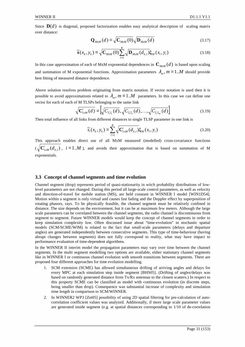
WINNER II D1.1.1 V1.1
Page 31 (153)
Since )(dD is diagonal, proposed factorization enables easy analytical description of scaling matrix
over distance:
)()0()( dd MxMMxMMxM DCQ = (3.17)
),()()0(),(~1
, llM
K
llkMxMMxMkk yxdyx ξDCs ∑
== (3.18)
In this case approximation of each of MxM exponential dependences in )(dMxMC is based upon scaling
and summation of M exponential functions. Approximation parameters Mmm ..1, =λ should provide
best fitting of measured distance dependence.
Above solution resolves problem originating from matrix notation. If vector notation is used then it is
possible to avoid approximations related to Mmm ..1, =λ parameters. In this case we can define one
vector for each of each of M TLSPs belonging to the same link
[ ])(,,)(,)()( ~~~~~~1 21dCdCdCd
Miii ssssssixM K=C (3.19)
Then total influence of all links from different distances to single TLSP parameter in one link is
),()(),(~1
,1 llM
K
llk
ixMkki yxdyxs ξC∑
== (3.20)
This approach enables direct use of all MxM measured (modelled) cross-covariance functions
( )( ,1 lkixM dC , Mi ..1= ), and avoids their approximation that is based on summation of M
exponentials.
3.3 Concept of channel segments and time evolution
Channel segment (drop) represents period of quasi-stationarity in witch probability distributions of low-level parameters are not changed. During this period all large-scale control parameters, as well as velocity and direction-of-travel for mobile station (MS), are held constant in WINNER I model [WIN1D54]. Motion within a segment is only virtual and causes fast fading and the Doppler effect by superposition of rotating phasors, rays. To be physically feasible, the channel segment must be relatively confined in distance. The size depends on the environment, but it can be at maximum few meters. Although the large scale parameters can be correlated between the channel segments, the radio channel is discontinuous from segment to segment. Future WINNER models would keep the concept of channel segments in order to keep simulation complexity low. Often discussed issue about “time-evolution” in stochastic spatial models (SCM/SCME/WIM) is related to the fact that small-scale parameters (delays and departure angles) are generated independently between consecutive segments. This type of time-behaviour (having abrupt changes between segments) does not fully correspond to reality, what may have impact to performance evaluation of time-dependent algorithms.
In the WINNER II interim model the propagation parameters may vary over time between the channel segments. In the multi segment modelling two options are available, either stationary channel segments like in WINNER I or continuous channel evolution with smooth transitions between segments. There are proposed four different approaches for time evolution modelling.
1. SCM extension (SCME) has allowed simultaneous drifting of arriving angles and delays for every MPC at each simulation step inside segment [BHS05]. (Drifting of angles/delays was based on randomly generated distance from Tx/Rx antennas to the closest scatters.) In respect to this property SCME can be classified as model with continuous evolution (in discrete steps, being smaller than drop). Consequence was substantial increase of complexity and simulation time length in comparison to SCM/WINNER.
2. In WINNER2 WP3 [Zet05] possibility of using 2D spatial filtering for pre-calculation of auto-correlation coefficient values was analyzed. Additionally, if more large scale parameter values are generated inside segment (e.g. at spatial distances corresponding to 1/10 of de-correlation

WINNER II D1.1.1 V1.1
Page 32 (153)
distance) 2D filtering would result in smooth transition between drops. Additionally it is necessary to provide smooth mapping of LSP into low-level parameters (delay, angles).
3. In this report the time evolution of propagation parameters is modelled like depicted in Figure 3-5. The route to be modelled is covered by adjacent channel segments. The distance between segments is equal to the stationarity interval. Transition from segment to segment is carried out by replacing clusters of the “old” segment by the clusters of the “new” segment, one by one. The route between adjacent channel segments is divided to number of sub-intervals equal to maximum number of clusters within the channel segments. During each sub-interval the power of one old cluster ramps down and one new cluster ramps up. Power ramps are linear. Clusters from the old and new segments are coupled based on their power. If number of clusters is different in the channel segments the weakest clusters are ramped up or down without a pair from other cluster.
4. The new approach is based on controlled positioning of clusters in (delay, angular) domain. As a control property existing LSP parameters (delay and angular spreads) and power distribution functions (marginal PDP, PAS or joint distribution) could be used. The only change to the existing situation would be that exact values of DS and AS would be enforced from delays, angles and power distributions.
time
delay
amplitude
Figure 3-5 Smooth transition between channel segments by power ramp-up and ramp-down of clusters.
Out of these four approaches, the two latter ones enable transitions between different propagation conditions, LOS/NLOS, and different propagation scenarios, e.g. outdoor/indoor. The third approach is chosen for WINNER2 interim model because of its relative simplicity. Anyhow the fourth approach will be studied further for the final model. It is outlined in the following:
1. When change in LS parameters (DS, AS) is small, that usually means that changes in cluster delays and angles are not significant (they are caused by the same scatterers like in previous drop). In this case quasi-deterministic approach based on distance from scatters could be applied ONCE at the initiation of the new drop, or small random offset can be applied.
2. When significant change in LSP is present, in reality we usually have different scatters (and possibly different number). In this case we have either to disposition existing clusters significantly or change the total number of clusters.
a. Number of scatters and changes in cluster delays and angles are not independent from LSP change! This will influence cluster life-time and has to be taken info account if concepts of cluster birth and death are to be supported by the WINNER. Necessity to remove or add new clusters should be based on properties acquired from measurement data, and it is highly probable that probability distributions related to number of clusters (as well as the other cluster properties) would be conditioned on LSP. For the each newly introduced cluster position (delay, angle) and power should be adjusted according to AS and DS values.
b. However changes in DS and AS could be described also by relocation of clusters. In this case clusters would be relocated sequentially (one-by-one) until exact values of DS and ASs are not obtained.
i. Processing starts in delay-domain by generating delays nτ from appropriate
probability distribution parameterized by DS and proportionality factor.

WINNER II D1.1.1 V1.1
Page 33 (153)
ii. Cluster powers 1010)(nSF
nn PDPP−
⋅= τ are obtained from PDP (also
controlled by DS). Additionally, per-cluster shadowing is included to describe measured deviations from PDP model.
iii. If calculated DS is different from required value, we are starting sequential relocation of clusters in delay domain. When relocating one cluster, its new
position in delay nτ and power )( nnP τ have to be determined. Since
calculated measure of delay spread is non-linear function of nτ :
))(,ds( nnn P ττ , we have to find solutions to non-linear equation
0))(,ds(DS =− nnn P ττ . If solution exist than relocation is over and
required value of DS is enforced. If equation does not have acceptable solution, we can move chosen cluster in such a manner to reduce difference between wanted and existing measures of DS, and after that proceed with next cluster. After relocating few clusters this procedure gives delays and powers that fulfil exact DS measure.
iv. Transition from delay domain to angular domains (departure and arrival) is based on powers determined in delay domain. The power angular spectrum
(PAS) is used to inversely map powers to angles: )(PAS 1nn P−=ϕ . (Inverse
mapping is not unique – it can not distinguish between left and right angle offsets in respect to LOS direction, but that is not important for this purpose). Obtained angles are initial since AS value calculated from these initial angles and powers may not be desired one.
v. To fit desired value of AS we can not change powers since they are related to desired DS. Instead, we have to adjust angles. Changes in angles are possible if deviations from PAS due to per-cluster shadowing are allowed. In our case we would assume that given power already includes shadowing what allows change of angle to certain extent (see the figure below)
nP
nϕ
10max 10
)( minnSF
nPϕ
−
10max 10
)( maxnSF
nPϕ−
maxnϕmin
nϕ vi. Procedure to fit required value of spread would be similar to that in delay
domain. Only difference is that during adjustment of angular spread, powers
are fixed and fitting is based only on angle values: 0)as(AS =− nϕ .
3.4 Reduced complexity models
A need has been identified for reduced-complexity channel models that can be used in rapid simulations having the objective of making comparisons between link-level systems alternatives (e.g. modulation and coding choices). In this report, such models are referred to as reduced-complexity models, and have the character of the well-known tapped delay line class of fading channel models. However, to address the needs of MIMO channel modelling, temporal variations at the taps are determined by more detailed information than that required for the specification of relative powers, envelope fading distributions, and fading rates, which are typical inputs to traditional tapped delay line models.
Specifically, multipath AoD and AoA information is inherent in the determination of tap fading characteristics. For these reasons, the reduced complexity models reported herein are referred to as

WINNER II D1.1.1 V1.1
Page 34 (153)
Cluster Delay Line (CDL) models. A cluster is centred at each tap. In general, each cluster is comprised of the vector sum of equal-powered MPCs (sinusoids), all of which have the same delay. Each MPC has a varying phase, but has fixed AoA and AoD offsets. The latter depend on the angular spreads at the MS and the BS, respectively, as shown in Table 3.10 of [WIN1 D5.4]. The values in this table were chosen to realise a specified Laplacian PAS for each cluster, appropriate to the scenario being modelled. In cases where there is a desire to simulate Ricean-like fading, an extra MPC is added, which is given a power appropriate to the desired Rice factor, and zero angular offset. The powers and delays of the clusters can be non-uniform, and can be chosen to realise the desired overall channel rms delay spread. Parameters of all CDL models reflect the expected values of those used in the more complex models described in other sections of this report.
Doppler information is not specified explicitly for CDL models. This is because it is determine by the AoAs of the MPCs, and the specified antenna patterns at the MS and BS, upon which there are no restrictions, except in fixed feeder link scenarios, as discussed in Section 3.4.2, below.
3.4.1 Cluster Delay Line models for mobile and portable scenarios The average power, mean AoA, mean AoD, and angle spreads at the BS and MS associated with each cluster within the cluster delay line models appropriate to scenarios A1, C2, and D1 were estimated from 100 Mchps channel sounding measurements at 5 GHz. Those for scenario B1 were estimated from 60 Mchps channel sounding measurements at 5 GHz. Tables of CDL parameters for the above-cited scenarios can be found in Section 4.
3.4.2 Cluster Delay Line models fixed feeder links Only CDL models have been created for fixed feeder links. Model parameters were derived from the literature, and are given in the tables of Section 4. As for the mobile and portable scenarios, any desired antenna patterns can be chosen. However, for B5 scenarios, at distances greater than 300 metres, the 3 dB beamwidth of the antenna at one end of the link should be less than 10 degrees, while that at the other end of the link should be less than 53 degrees. Different parameters are specified in the cited tables for scenarios B5a, b, c, and d.
For fixed link scenarios, Doppler shifts are independent of AOAs. Instead, they are derived from considerations concerning the movement of interacting objects. One interacting object per cluster is modelling as having motion, while the others are fixed. Associated Doppler frequencies are specified in CDL tables.
3.4.3 Cluster delay line models for fixed multi-hop scenarios In multi-hop (e.g. B5f) scenarios, the radio waves can take a route between successive MS. Relaying networks, on the other hand, employ another level of network stations, the relays, which depending on the specific network, might offer more or less functionality to distribute traffic intelligently. This means the existence of scenarios where multiple relay nodes are receiving and transmitting the data towards its final destination, as shown in Figure 3-6.
Figure 3-6 Multihop and relaying scenarios.
Fixed propagation parameters like delay, power, AoA and AoD are tabulated in section 4. The clustered structure of energy from scatterers is assumed. Models for such scenarios are composed of e.g. 20 clusters, with a number of MPCs per cluster. One MPC per cluster is virtually in motion and energy

WINNER II D1.1.1 V1.1
Page 35 (153)
received from it has a predetermined Doppler frequency. The remaining energy is from physically stationary interacting objects.
The Power delay profile model is exponential. Delay spread values are determined by channel measurements. As above, the CDL model for this scenario can be used in conjunction with any antenna configuration for the generation of radio channel realisations.

WINNER II D1.1.1 V1.1
Page 36 (153)
4. Channel Models and Parameters In this section, we summarize all the channel models and parameters derived so far, and the measurement scenarios include both old and new measurement campaigns performed in Phase I and II. The path loss models were mainly based on 5 GHz and 2 GHz measurements. However, the frequency bands have been extended in 2 ~ 6 GHz. In the parameter tables for the generic models, parameters for far clusters and the correlations of polarization are added. For CDL models, in Phase I, the link level empirical models were derived based on measurements. In Phase II, we use simulation method and the real number of clusters by measurements, new CDL models are obtained. Moreover, the comparisons between Phase I and Phase II generic and CDL models are given.
4.1 Applicability
4.1.1 Environment dependence Different radio-propagation environment would cause different radio-channel characteristics. Instead of attempt to parameterize environment directly (e.g. street widths, average building height etc.) WINNER models are using (temporal and spatial) propagation parameters obtained from channel measurements in different environments. In this context, environments in which measurements are conduced to observe radio-channel characteristics are called scenarios. For each scenario measured data is analyzed and processed to obtain scenario-specific parameters. After this point, same generic channel is used to model all scenarios, just by using different values of control parameters.
Usually, even for the same scenario, existence of LOS component substantially influences values of control parameters. Regarding to this property, each WINNER scenario is differentiating between LOS and NLOS conditions. To enable appropriate scenario modelling, transition between LOS and NLOS cases have to be described. For this purpose distance dependent probability of LOS and Ricean K factors are used in the model.
4.1.2 System dependence Dependence on carrier frequency in WINNER model is found in path-loss models. All the scenarios defined by WINNER support frequency dependent path-loss models valid for the ranges of 2 – 6 GHz. The path-loss models are based on measurements that are mainly conducted in 5 GHz frequency range.
From WINNER measurement results and literature survey it was found that model parameters DS, AS and Ricean K-factor do not show significant frequency dependence [BHS05]. From that reason these parameters show only dependence on environment (scenario).
For modelling of systems with time-division-duplex (TDD) all models are using same (large-scale as small-scale) parameters for both uplink and downlink. If system is using different carriers for duplexing (FDD), then (additionally to path loss) random phases of scatterer contributions between UL and DL are independent.
For the WINNER purposes it is required that channel model supports bandwidths up to 100 MHz. Following the approach described in [SV87] (for indoor propagation modelling) and further with SCME [BHS05] WINNER II model introduces intra-cluster delay spread as a mean to support 100 MHz bandwidth and to suppress frequency correlation. Instead of zero-delay-spread-cluster approach of Phase I model, the two strongest clusters with 20 MPCs is subdivided into 3 zero-delay sub-clusters. Thus we keep the total number of MPCs constant, but introduce four additional delay taps per scenario.
4.2 Generation of Channel Coefficients
This section gives general description of the channel coefficient generation procedure. Steps of the procedure refer to parameter and model tables of Section 0. Sections 4.2 to 4.4 give the minimum description of the system level channel model.
It has to noted, that the geometric description covers arrival angles from the last bounce scatterers and respectively departure angles to the first scatterers interacted from the transmitting side. The propagation between the first and the last interaction is not defined. Thus this approach can model also multiple interactions with the scattering media. This indicates also that e.g. the delay of a multipath component can not be determined by the geometry.

WINNER II D1.1.1 V1.1
Page 37 (153)
General parameters:
Step 1: Set environment, network layout and antenna array parameters
a. Choose one of the scenarios (A1, A2, B1,…) b. Give number of BS and MS c. Give locations of BS and MS, or equally distances of each BS and MS and relative
directions ϕLOS and φLOS of each BS and MS d. Give BS and MS antenna field patterns and array geometries e. Give BS and MS array orientations with respect to north (reference) direction f. Give speed and direction of motion of MS g. Give system centre frequency h. Give antenna field patterns Frx and Ftx
Large scale parameters: Step 2: Assign propagation condition (LOS/NLOS) according to the probability described in Table 4-7. Step 3: Calculate path loss with formulas of Table 4-4 for each BS-MS link to be modelled. Step 4: Generate correlated large scale parameters, i.e. delay spread, angular spreads and shadow fading term like explained in section 3.2.1 (Correlations between large scale parameters). Small scale parameters:
Step 5: Generate delays τ. Delays are drawn randomly from delay distribution defined in Table 4-5. With exponential delay distribution calculate
( )nn Xr log' ττστ −= , (4.1)
where rτ is delay distribution proportionality factor, Xn ~ Uni(0,1) and cluster index n = 1,…,N. With
uniform delay distribution the delay values τn’ are drawn from the corresponding range. Normalise the delays by subtracting with minimum delay and sort the normalised delays to descending order.
( )( )'min'sort nnn τττ −= . (4.2)
In the case of LOS condition additional scaling of delays is required to compensate the effect of LOS peak addition to the delay spread. Heuristically determined Ricean K-factor dependent scaling constant is
32 000017.00002.00433.07705.0 KKKD ++−= , (4.3)
where K [dB] is the Ricean K-factor defined in Table 4-5. Scaled delays are
DnLOSn /ττ = , (4.4)
they are not to be used in cluster power generation.
Step 6: Generate cluster powers P. Cluster powers are calculated assuming a single slope exponential power delay profile. Power assignment depends on the delay distribution defined in Table 4-5. With exponential delay distribution the cluster powers are determined by
10' 101
expn
r
rP nn
Ζ−
⋅
−−=ττ
τ
στ (4.5)
and with uniform delay distribution they are determined by
10' 10expn
nnP
Ζ−
⋅
−=τστ
, (4.6)
where Ζn ~ N(0, ζ ) is the per cluster shadowing term in [dB]. Average the power so that sum power of all clusters is equal to one
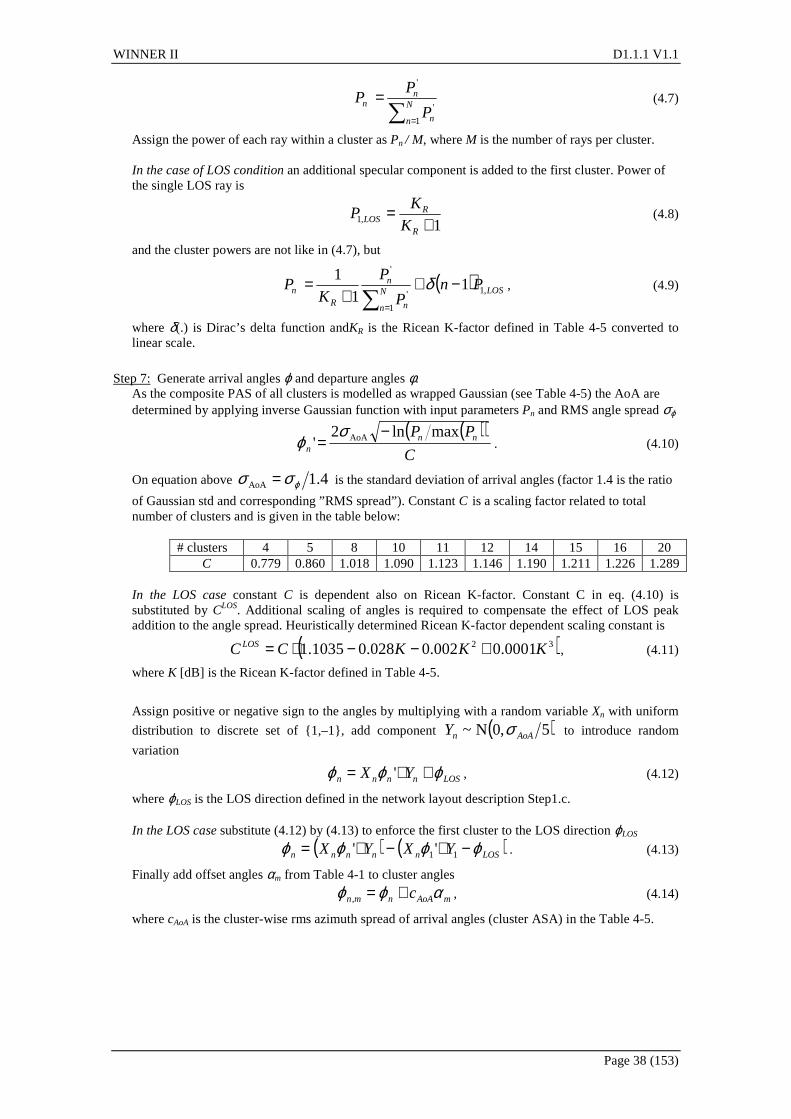
WINNER II D1.1.1 V1.1
Page 38 (153)
∑ =
= N
n n
nn
P
PP
1
'
'
(4.7)
Assign the power of each ray within a cluster as Pn / M, where M is the number of rays per cluster. In the case of LOS condition an additional specular component is added to the first cluster. Power of the single LOS ray is
1,1 +
=R
RLOS K
KP (4.8)
and the cluster powers are not like in (4.7), but
( ) LOSN
n n
n
Rn Pn
P
P
KP ,1
1
'
'
11
1 −++
=∑ =
δ , (4.9)
where δ(.) is Dirac’s delta function andKR is the Ricean K-factor defined in Table 4-5 converted to linear scale.
Step 7: Generate arrival angles ϕ and departure angles φ.
As the composite PAS of all clusters is modelled as wrapped Gaussian (see Table 4-5) the AoA are determined by applying inverse Gaussian function with input parameters Pn and RMS angle spread σϕ
( )( )
C
PP nnn
maxln2' AoA −=
σϕ . (4.10)
On equation above 4.1AoA ϕσσ = is the standard deviation of arrival angles (factor 1.4 is the ratio
of Gaussian std and corresponding ”RMS spread”). Constant C is a scaling factor related to total number of clusters and is given in the table below:
# clusters 4 5 8 10 11 12 14 15 16 20 C 0.779 0.860 1.018 1.090 1.123 1.146 1.190 1.211 1.226 1.289
In the LOS case constant C is dependent also on Ricean K-factor. Constant C in eq. (4.10) is substituted by CLOS. Additional scaling of angles is required to compensate the effect of LOS peak addition to the angle spread. Heuristically determined Ricean K-factor dependent scaling constant is
( )32 0001.0002.0028.01035.1 KKKCCLOS +−−⋅= , (4.11)
where K [dB] is the Ricean K-factor defined in Table 4-5.
Assign positive or negative sign to the angles by multiplying with a random variable Xn with uniform
distribution to discrete set of 1,–1, add component ( )5,0N~ AoAnY σ to introduce random
variation
LOSnnnn YX ϕϕϕ ++= ' , (4.12)
where ϕLOS is the LOS direction defined in the network layout description Step1.c. In the LOS case substitute (4.12) by (4.13) to enforce the first cluster to the LOS direction ϕLOS
( ) ( )LOSnnnnn YXYX ϕϕϕϕ −+−+= 11'' . (4.13)
Finally add offset angles αm from Table 4-1 to cluster angles
mAoAnmn c αϕϕ +=, , (4.14)
where cAoA is the cluster-wise rms azimuth spread of arrival angles (cluster ASA) in the Table 4-5.

WINNER II D1.1.1 V1.1
Page 39 (153)
Table 4-1 Ray offset angles within a cluster, given for 1°°°° rms angle spread.
Ray number m Basis vector of offset angles αm 1,2 ± 0.0447 3,4 ± 0.1413 5,6 ± 0.2492 7,8 ± 0.3715 9,10 ± 0.5129 11,12 ± 0.6797 13,14 ± 0.8844 15,16 ± 1.1481 17,18 ± 1.5195 19,20 ± 2.1551
For the departure angles φn the procedure is analogous.
Step 8: Random coupling of rays within the clusters.
Couple randomly departure ray angles φn,m to arrival ray angles ϕn,m within a cluster n, or within a sub-cluster in the case of two strongest clusters (see step 11 and Table 4-2).
Step 9: Generate vertical-to-horizontal and horizontal-to-vertical cross polarisation power ratios (XPR) κvh and κhv respectively for each ray m of each cluster n.
XPR is log-Normal distributed. Draw vertical-to-horizontal XPR values as
10vh, 10Xnm =κ , (4.15)
where ray index m = 1,…,M, X ~ N(σ,µ) is Gaussian distributed with σ and µ from Table 4-5 for XPRVH. For the horizontal-to-vertical XPR the procedure is analogous.
Coefficient generation:
Step 10: Draw random initial phase hh,
hv,
vh,
vv, ,,, mnmnmnmn ΦΦΦΦ for each ray m of each cluster n and for
four different polarisation combinations (vv,vh,hv,hh). Distribution for initial phases is uniform, Uni(-π,π). Step 11: Generate channel coefficients for each cluster n and each receiver and transmitter element pair u,s.
For the N – 2 weakest clusters, say n = 3,4,…,N, and uniform linear arrays (ULA), the channel coefficient are given by:
( ) ( )
( )( ) ( )
( ) ( )( )( )
( )( ) ( )( ) ( )tjjdjd
F
F
jj
jj
F
FPt
mnmnumns
mnHstx
mnVstx
hhmn
hvmn
hvmn
vhmn
vhmn
vvmn
T
mnHurx
mnVurxM
mnnsu
,,1
0,1
0
,,,
,,,
,,,
,,,
,,,
,,,
1,,
2expsin2expsin2exp
expexp
expexp
πυϕπλφπλ
ϕϕ
κκ
φφ
−−
=
⋅
ΦΦ
ΦΦ
= ∑H
(4.16)
where Frx,u,V and Frx,u,H are the antenna element u field patterns for vertical and horizontal polarisations respectively, ds and du are the uniform distances [m] between transmitter elements and receiver elements respectively, and λ0 is the wave length on carrier frequency. If polarisation is not considered, 2x2 polarisation matrix can be replaced by scalar ( )mnj ,exp Φ and only vertically
polarised field patterns applied.
With fixed feeder link models (B5 scenarios) the Doppler frequency component νn,m is tabulated for the first ray of each cluster. For the other rays νn,m = 0. With all other models the Doppler frequency component is calculated from angle of arrival (downlink), MS speed v and direction of travel θv
( )
0
,,
cos
λθϕ
υ vmnmn
v −= , (4.17)
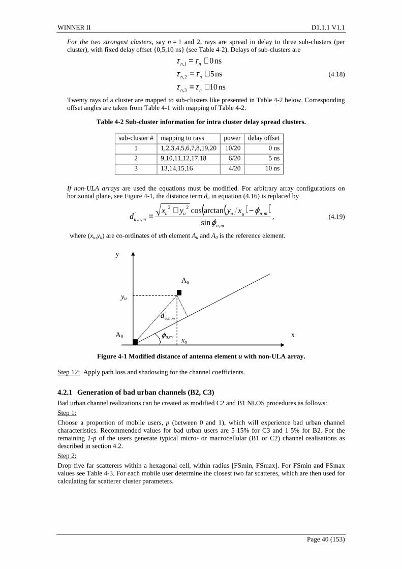
WINNER II D1.1.1 V1.1
Page 40 (153)
For the two strongest clusters, say n = 1 and 2, rays are spread in delay to three sub-clusters (per cluster), with fixed delay offset 0,5,10 ns (see Table 4-2). Delays of sub-clusters are
ns10
ns5
ns0
3,
2,
1,
+=+=+=
nn
nn
nn
ττττττ
(4.18)
Twenty rays of a cluster are mapped to sub-clusters like presented in Table 4-2 below. Corresponding offset angles are taken from Table 4-1 with mapping of Table 4-2.
Table 4-2 Sub-cluster information for intra cluster delay spread clusters.
sub-cluster # mapping to rays power delay offset
1 1,2,3,4,5,6,7,8,19,20 10/20 0 ns
2 9,10,11,12,17,18 6/20 5 ns
3 13,14,15,16 4/20 10 ns
If non-ULA arrays are used the equations must be modified. For arbitrary array configurations on horizontal plane, see Figure 4-1, the distance term du in equation (4.16) is replaced by
( )( )
mn
mnuuuumnu
xyyxd
,
,22
',, sin
arctancos
ϕϕ−+
= , (4.19)
where (xu,yu) are co-ordinates of uth element Au and A0 is the reference element.
ϕn,m
du’
yu
xu A0
Au
y
x
',, mnud
Figure 4-1 Modified distance of antenna element u with non-ULA array.
Step 12: Apply path loss and shadowing for the channel coefficients.
4.2.1 Generation of bad urban channels (B2, C3) Bad urban channel realizations can be created as modified C2 and B1 NLOS procedures as follows:
Step 1:
Choose a proportion of mobile users, p (between 0 and 1), which will experience bad urban channel characteristics. Recommended values for bad urban users are 5-15% for C3 and 1-5% for B2. For the remaining 1-p of the users generate typical micro- or macrocellular (B1 or C2) channel realisations as described in section 4.2.
Step 2:
Drop five far scatterers within a hexagonal cell, within radius [FSmin, FSmax]. For FSmin and FSmax values see Table 4-3. For each mobile user determine the closest two far scatteres, which are then used for calculating far scatterer cluster parameters.
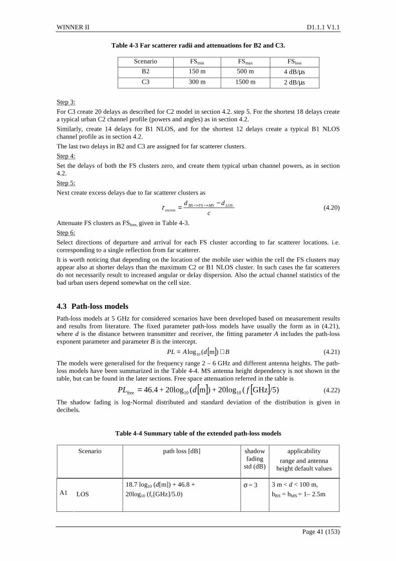
WINNER II D1.1.1 V1.1
Page 41 (153)
Table 4-3 Far scatterer radii and attenuations for B2 and C3.
Scenario FSmin FSmax FSloss
B2 150 m 500 m 4 dB/µs
C3 300 m 1500 m 2 dB/µs
Step 3:
For C3 create 20 delays as described for C2 model in section 4.2. step 5. For the shortest 18 delays create a typical urban C2 channel profile (powers and angles) as in section 4.2.
Similarly, create 14 delays for B1 NLOS, and for the shortest 12 delays create a typical B1 NLOS channel profile as in section 4.2.
The last two delays in B2 and C3 are assigned for far scatterer clusters.
Step 4:
Set the delays of both the FS clusters zero, and create them typical urban channel powers, as in section 4.2.
Step 5:
Next create excess delays due to far scatterer clusters as
c
dd LOSMSFSBSexcess
−= >−>−τ (4.20)
Attenuate FS clusters as FSloss, given in Table 4-3.
Step 6:
Select directions of departure and arrival for each FS cluster according to far scatterer locations. i.e. corresponding to a single reflection from far scatterer.
It is worth noticing that depending on the location of the mobile user within the cell the FS clusters may appear also at shorter delays than the maximum C2 or B1 NLOS cluster. In such cases the far scatterers do not necessarily result to increased angular or delay dispersion. Also the actual channel statistics of the bad urban users depend somewhat on the cell size.
4.3 Path-loss models
Path-loss models at 5 GHz for considered scenarios have been developed based on measurement results and results from literature. The fixed parameter path-loss models have usually the form as in (4.21), where d is the distance between transmitter and receiver, the fitting parameter A includes the path-loss exponent parameter and parameter B is the intercept.
[ ] BdAPL += )m(log10 (4.21)
The models were generalised for the frequency range 2 – 6 GHz and different antenna heights. The path-loss models have been summarized in the Table 4-4. MS antenna height dependency is not shown in the table, but can be found in the later sections. Free space attenuation referred in the table is
[ ] [ ]/5)GHz(20log+)m(20log+46.4 1010free fdPL = (4.22)
The shadow fading is log-Normal distributed and standard deviation of the distribution is given in decibels.
Table 4-4 Summary table of the extended path-loss models
Scenario path loss [dB] shadow fading
std (dB)
applicability
range and antenna height default values
A1 LOS
18.7 log10 (d[m]) + 46.8 +
20log10 (fc[GHz]/5.0) σ = 3 3 m < d < 100 m,
hBS = hMS = 1– 2.5m

WINNER II D1.1.1 V1.1
Page 42 (153)
NLOS (Room- Corridor)
NLOS (Room-Room trough wall)
PL = 36.8 log10 (d[m]) + 43.8 +
20log10 (f [GHz]/5.0)
PL = 20 log10 (d[m]) + 46.4 +
nW · 5 + 20log10 (f [GHz]/5.0)
PL = 20 log10 (d[m]) + 46.4 +
nW · 12 + 20log10 (f[GHz]/5.0)
where nw is the number of
walls between BS and MS.
σ = 4
σ = 6
σ = 8
3 m < d < 100 m,
hBS = hMS = 1– 2.5m
3 m < d < 100 m
(light walls),
hBS = hMS = 1– 2.5m
3 m < d < 100 m
(heavy walls),
hBS = hMS = 1– 2.5m
A2 NLOS
PL = PLb + PLtw + PLin where
PLb = PLB1(dout + din) ,
PLtw = 14 + 15(1 - cos(θ))2 ,
PLin = 0.5 din
σ = 7 3 m <dout+ din < 1000 m
hBS = 3nFl + 2 m
hMS = 1.5 m
See 1) for explanation of parameters
LOS
PLLOS = max(22.7 log10 (d1 [m]) + 41.0 + 20 log10 (f [GHz]/5.0), PLFree)
PLLOS = 40.0 log10 (d1 [m]) + 9.45 - 17.3log10 (h’BS [m]) +
- 17.3log10 (h’MS [m]) +
+2.7log10(f [GHz]/5.0)
σ = 3
σ = 3
30 m < d1 < d’BP2)
hBS = 10 m
hMS = 1.5 m
d’BP < d1 < 5 km
B1
NLOS
PLNLOS = PLLOS(d1) + 20 – 12.5·nj + 10nj·log10 (d2[m])
where nj = max((2.8 – 0.0024d1[m]), 1.84)
σ = 4 10 m < d1 < 5 km,
w/2 < d2 < 2 km 3)
w =20m
hBS = 10 m
hMS = 1.5 m
B2 NLOS Same as B1.
LOS 13.4 log10 (d[m]) + 36.9 σ = 1.4 5 m < d < 29 m B3
NLOS 3.2 log10 (d[m]) + 55.5 σ = 2.1 5 m < d < 29 m
B4 NLOS
Same as A2,
except for antenna heights.
σ = 7 3 m <dout+ din < 1000 m
hBS = 10 m
hMS = 3nFl + 1.5 m
B5a LOS
PL = max(23.5 log10 (d) + 42.5 +
20 log10 (f [GHz]/5.0), PLFree)
σ = 4 30m < d <8km
hBS = 25 m
hMS = 25 m (= Relay antenna height)
B5c LOS
Same as B1 LOS,
except for the antenna height of the Relay Station (See the rightmost column.).
σ = 3
hBS = 10 m
hMS (=hRS) = 5 m
(Relay antenna height)

WINNER II D1.1.1 V1.1
Page 43 (153)
B5f NLOS
PL = 23.5 log10 (d) + 57.5 +
20 log10 (f [GHz]/5.0)
σ = 8 30m < d < 1.5 km
hBS = 25 m
hRS = 15 m (= Relay antenna height)
LOS
PL = 23.8 log10 (d [m]) + 41.2 +
20 log10 (f [GHz]/5.0)
PL = 40.0 log10 (d [m]) +
11.65 - 16.2log10 (hBS [m])
- 16.2log10 (hMS [m]) +
3.8log10(f [GHz]/5.0)
σ = 4
σ = 6
30 m < d < dBP 4)
hBS = 25 m
hMS = 1.5 m
dBP < d < 5 km
C1
NLOS
PL = [44.9-6.55log10(hBS[m])]log10(d[m]) + 31.46 + 5.83log10(hBS[m]) + 20log10(f [GHz]/5.0)
σ = 8 50 m < d < 5 km
hBS = 25 m
hMS = 1.5 m
C2 NLOS
PL = [44.9-6.55log10(hBS[m])]log10(d[m]) + 34.46 + 5.83log10(hBS[m]) + 20log10(f [GHz]/5.0)
σ = 8 50 m < d < 5 km
hBS = 25 m
hMS = 1.5 m
C3 Same as C2.
LOS
PL = 44.2 + 21.5 log10(d) + 20 log10(f [GHz]/5)
PL = 10.5 + 40.0 log10 (d1 [m]) - 18.5log10(hBS[m]) - 18.5log10 (hMS [m]) + 1.5log10(f [GHz]/5)
σ = 4
σ = 6
30 m < d < dBP4)
hBS = 32 m
hMS = 1.5 m
dBP < d < 10 km,
D1
NLOS
PL = max((55.4+25.1log10(d[m])
-0.13log10(hBS[m]-25))log10 (d[m]/100)
- 0.9(hMS[m]-1.5) +
21.3 log10(f [GHz]/5.0), PLFree)
σ = 8 50 m < d < 5 km
hBS = 32 m
hMS = 1.5 m
D2a LOS
PL = max(41.1 log10(d)+17.2
+ 20log10(f [GHz]/5.0) , PLFree) σ = 3 30 m < d < 2 km
hBS = 6 m
hMS = 5 m
1) PLB1 is B1 path-loss, dout is the distance between the outside terminal and closest point of the wall to the inside terminal, din is the distance from wall to the inside terminal , θ is the angle between the outdoor path and the normal of the wall. (See 6.2.1.) nFl is the number of the floor. (Ground floor is the number 1.)
2) d’BP = 4 h’BS h’MS f/c, where f = center frequency and c = velocity of light and h’BS and h’MS
are the effectice antenna heights at BS and MS respectively: h’BS = hBS-1.0 m, h’MS = hMS – 1.0 m, where 1.0 m is the effective environment height in the urban environment.
3) d1 and d2 have been explained below. 4) dBP
= 4 hBS hMS f/c,, where hBS and hMS are the actual antenna heights
For B1, we have developed d1 and d2 path loss model for NLOS. For A1, the similar path-loss model can be derived, but it can be applied for the whole crossing of the corridors. The geometry for the d1 and d2 models is shown in Figure 4-2 where the BS is located in one street/corridor and the MS is moving in the perpendicular street /corridor. d1 is the distance from the BS to the middle point of the street/corridor and d2 is the distance apart from the middle point of the crossing of the MS.

WINNER II D1.1.1 V1.1
Page 44 (153)
BSd 1
d
d
2
2
MS
+
-
Figure 4-2 Geometry for d1 and d2 path-loss model
4.4 Parameter tables for generic models

WINNER II D1.1.1 V1.1
Page 45 (153)
Table 4-5 Parameter table for generic models in azimuth plane.
A1 A2 B1 B3 B4 C1 C2 D1 D2a Scenarios
LOS NLOS NLOS LOS NLOS LOS NLOS NLOS LOS NLOS NLOS LOS NLOS LOS µ -7.42 -7.60 -7.40 -7.44 -7.12 -7.55 -7.40 -7.31 -7.23 -7.12 -6.63 -7.80 -7.60 -7.4 Delay spread σDS
log10([s]) σ 0.27 0.19 0.18 0.25 0.12 0.10 0.19 0.36 0.49 0.33 0.32 0.57 0.48 0.2 µ 1.64 1.73 1.71 0.40 1.19 1.48 1.07 1.08 0.78 0.90 0.93 0.78 0.96 1.07 AoD spread σASD
++ log10([°]) σ 0.31 0.23 0.16 0.37 0.21 0.21 0.14 0.42 0.12 0.36 0.22 0.21 0.45 0.31
µ 1.65 1.67 1.25 1.40 1.55 1.15 1.60 1.76 1.48 1.65 1.72 1.20 1.52 1.5 AoA spread σASA log10([°]) σ 0.26 0.14 0.41 0.20 0.20 0.26 0.24 0.14 0.20 0.30 0.14 0.18 0.27 0.1 Shadow fading σSF [dB] σ 3 6 7 3 4 2 2 7 4/6 + 8 8 4/6 + 8 2.5
σASD vs σDS 0.5 -0.1 0.4 0.5 0.2 0.2 0.1 0.3 0.3 0.3 0.4 0.1 -0.4 0.1 σASA vs σDS 0.7 0.3 0.4 0.8 0.4 -0.2 0.5 0 0.8 0.7 0.6 0.2 0.1 0.2 σASA vs σSF -0.4 -0.4 0.1 -0.5 -0.4 -0.2 0.1 0 -0.2 -0.3 -0.3 -0.1 0.1 -0.1 σASD vs σSF -0.1 0 0 -0.5 0 -0.3 -0.2 -0.3 0.4 -0.4 -0.6 -0.1 0.6 -0.1 σDS vs σSF -0.7 -0.5 -0.2 -0.4 -0.7 0.2 0.3 0.5 -0.7 -0.4 -0.4 -0.7 -0.5 -0.7
Cross-Correlations **
σASD vs σASA 0.4 -0.3 0.1 0.4 0.1 0.0 0.3 -0.1 0.3 0.3 0.4 -0.5 -0.2 -0.5
Delay distribution Exp Exp Exp Exp Uniform ≤800ns
Exp Exp Exp Exp Exp Exp Exp Exp Exp
Delay scaling parameter rτ 3 2.4 2.2 3.2 1.9 1.6 1.8 2.4 1.5 2.3 3.8 1.7 3.8 µ 11.4 9.7 8.1 8.6 8.0 0.5 0.1 4.0 7.9 3.3 7.6 6.9 7.9 6.9
XPRV [dB] σ 3.4 3.5 10.4 1.8 1.8 1.1 0.7 11.2 3.3 2.5 3.4 2.3 3.5 2.3 µ 10.4 10.0 8.5 9.5 6.9 N/A* N/A 9.5 3.7 5.7 2.3 7.2 7.5 7.2
XPRH [dB] σ 3.4 3.1 10.9 2.3 2.8 N/A N/A 11.3 2.5 2.9 0.2 2.8 4.0 2.8 AoD and AoA distribution Wrapped Gaussian Number of clusters 12 16 10 8 16 5 10 12 15 14 20 11 10 4 Number of rays per cluster 20 20 20 20 20 20 20 20 20 20 20 20 20 20 Cluster ASD 5 5 8 3 10 5 6 5 5 2 2 2 2 2 Cluster ASA 5 5 5 18 22 5 13 8 5 10 15 3 3 3 Per cluster shadowing std ζ [dB] 6 3 3 3 3 3 3 4 3 3 3 3 3 3
K-factor [dB] 8.3 –0.06d 3.2 3 +
0.0142d 6 –
0.26d 8.1 17.1 – 0.021d
3.7 + 0.02d 6
σDS 7 4 21 9 8 5 2 10 64 40 40 64 36 64 σASD 6 5 15 13 10 2 1 11 20 30 50 25 30 25 σASA 2 3 35 12 9 1 1 6 18 30 50 40 40 40
Correlation distance [m]
σSF 6 4 14 14 12 4 6 4 23 50 50 40 120 40
+ Scenarios C1 LOS and D1 LOS contain two shadowing std. deviations; one (left) for before and one (right) for after the path loss breakpoint. ++ Angle of departure spread σASD corresponds to σφ and angle of arrival spread σASA to σϕ in the text. * For scenario B3, XPRH is not available. In the channel model implementation, these values have bee substituted by the XPRV. ** The sign of the shadow fading is defined so that positive SF means more received power at MS than predicted by the path loss model.

WINNER II D1.1.1 V1.1
Page 46 (153)
Table 4-6 Parameter table for generic models in elevation plane.
A1 A2 B4 Scenarios
LOS NLOS NLOS NLOS
µ 0.88 1.06 0.88 1.01 Elevation AoD spread σESD
+ σ 0.31 0.21 0.31 0.43
µ 0.94 1.10 0.88 0.88 Elevation AoA spread σESA σ 0.26 0.17 0.34 0.34
σESD vs σDS 0.5 -0.6 N/A -0.18
σESA vs σDS 0.7 -0.1 0.3 N/A
σESA vs σSF -0.1 0.3 -0.2 N/A
σESD vs σSF -0.4 0.1 N/A -0.52
Cross-Correlations
σESD vs σESA 0.4 0.5 N/A N/A
Elevation AoD and AoA distribution
Wrapped Gaussian
Cluster ESD 3 3 3 3
Cluster ESA 3 3 3 3
+ Elevation angle of departure spread σESD corresponds to σθ and elevation angle of arrival spread σESA to σϑ in the text.
The output expectation values for LS parameters are given in section 4.4.1.
System level simulations require the probability of line of sight for considered scenarios. For scenarios A2, B2, B4, C2 and C3 the LOS probability is zero. For rest of the scenarios the probabilities are given in Table 4-7. It should be noted that the LOS probability models are based on relatively few data or are deduced using some simplified assumptions. Therefore these probabilities should be treated as only indicative.
In grid-based scenarios like A1 (indoor layout) and B1 (Manhattan grid) it is probably more favourable to define the position of mobiles respective to the APs using d1 – d2 distances as specified in connection of the path-loss definition, see Figure 4-2, or even x-y coordinates. Then it is easy to specify the LOS condition according to the position of the mobile and use it in defining the propagation connection of each link. One problem of LOS probability is that the location of APs affects the LOS probability in grid-based scenarios. Actually the LOS probabilities for A1 and B1 in Table 4-7 are possibly not fully consistent with the current evaluation assumptions.

WINNER II D1.1.1 V1.1
Page 47 (153)
Table 4-7 Line of sight probabilities
Scenario LOS probability as a function of distance d [m] Note
A1 ( )( )
>−−−
≤=
5.2,)(log61.024.119.01
5.2,1313
10 dd
dPLOS
B1
>≤
=10,20
10,1
dd
dPLOS
>
−−
≤=
10,45
10exp
10,1
dd
d
PLOS
For big factory halls, airport and train stations.
B3
<<
−−
≤=
405,150
5exp
5,1
dd
d
PLOS
For big lecture halls and conference halls.
C1
−=200
expd
PLOS
D1
−=1000
expd
PLOS
D2a Same as D1
4.4.1 Reference output values
Table 4-8: Expectation (median) output values for large scale parameters.
Scenario DS (ns) AS at BS (º) AS at MS (º) ES at BS (º) ES at MS (º) LOS 40 44 45 8 9
A1 NLOS 25 53 49 11 13
A2 NLOS 40 53 18 10 10
LOS 36 3 25 B1
NLOS 76 15 35
LOS 28 30 14
B3
NLOS 40 12 40
B4 NLOS 49 12 58 10 10
LOS 59 6 30
C1
NLOS 75 8 45
C2 NLOS 234 8 53
D1 LOS 16 6 16

WINNER II D1.1.1 V1.1
Page 48 (153)
NLOS 37 9 33
D2 LOS 39 5 30
For reference, the following table illustrates some output channel statistics (median values) for micro- and macrocellular bad urban mobile users. For the calculation max cell radii of 200 and 500 m were used for micro- and macrocells, respectively, and bad urban users were uniformly distributed within the cell area.
Table 4-9: Expectation (median) output values of large scale parameters for bad urban scenarios.
Scenario DS (µs) AS at BS (º)
AS at MS (º)
Power of the 1st FS cluster (dB)
Power of the 2nd FS cluster (dB)
Delay of the 1st FS cluster (µs)
Delay of the 2nd FS cluster (µs)
B2 0.48 33 51 -5.7 -7.7 1.1 1.6
C3 0.63 17 55 -9.7 -13.0 3.1 4.8
4.5 Transitions between propagation conditions
The channel model allows the transition between different propagation conditions: Most important is the transition between LOS and NLOS propagation conditions of same scenario. Another possible transition is from one scenario to another one. For two cases there is a path-loss model for the intra scenario transition: B1 urban microcell and A1 indoor (small office case). B1 path-loss model has been introduced in [WIN1D54] and Table 4-4 of this document. A1 model has been created during WINNER Phase II and is an extension to the earlier model in [WIN1D54]. Channel model is introduced in detail in Part II of the document. The formulas are:
[ ]
[ ] [ ]
≤+=++
<+−++=
1222
211010
12102101121
3,,5)GHz(log*20)(log*7.188.46
3,5)GHz(log*20)(log*)055.02.21(61.09.68),(
Fddddfmd
FdfdddddPL
c
c (4.23)
where d1 and d2 are the distances along the LOS route and perpendicular NLOS route and Wms is the
width of the corridor when MS is located. F1 is specified below:
21
11 22
1
−= msms W
d
WF λ (4.24)
For B1, the path-loss can be expressed as follows when a mobile is turning a strret corner from LOS/NLOS including the transition region
>+−+≤+==
122101
1222
21
2110),(log105.1220)(
10,),(),(
FddnndPL
FdddddPLddPL
LOS
LOS (4.25)
where
[ ]5/)GHz(log20)(log7.220.41)( 101101 fddPLLOS +⋅+= (4.26)
and 14
1 1025.52.3,*0024.08.2 ddn SF−×−=−= σ dB.
Fig 4-3 (a) and 4-3 (b) show the pathloss models including transition regions for A1 and B1, respectively.

WINNER II D1.1.1 V1.1
Page 49 (153)
(a) (b)
Figure 4-3 Examples of the path.loss models including the transitions. (a) A1. (b) B1
4.6 CDL Models
The CDL model is somehow different from the conventional tapped delay line models in a sense that fading within each tap is generated by a sum of sinusoids i.e., the rays within the cluster of that tap. However, it is based on similar principles of the clustered channel modelling approach. Clustered delay line (CDL) model is composed of a number of separate delayed clusters. Each cluster has a number of multipath components (rays) that have the same known delay values but differ in known angle of departure and known angle of arrival. The cluster angle-spread may be different from that of BS to that of the MS. The offset angles represent the Laplacian PAS of each cluster. The average power, mean AoA, mean AoD of clusters, angle-spread at BS and angle-spread at MS of each cluster in the CDL represent expected output of the stochastic model with parameters listed in Table 4-8. Exception to this are the fixed feeder link models (scenario B5), where only CDL model is defined.
Parameter tables for CDL models are given in Part II of this document.
4.7 Comparison of Phase I and Phase II models
This section shows the main differences between the Phase I (D5.4) and Phase II (D1.1.1) models.
Phase II models include more scenarios (A2, B2, C3, B4, B5f, D2a, and D2b) and more features like time evolution of large scale parameters, intra cluster delay spread, and far cluster option. CDL models are based on expectation values of the large scale parameters of the stochastic models. Time evolution is organized by replacing old clusters with new clusters one by one, with power ramp up and ramp down.
Table below shows which scenarios are available in Phase I and in Phase II models, respectively. Note that all the scenarios of Phase I have been updated in Phase II models.
Table 4-10 Availability of scenarios in Phase I and Phase II models
Scenario Phase I Phase II
code definition generic model
CDL generic model
CDL
A1 indoor small office yes yes yes yes
A2 indoor-to-outdoor yes yes
B1 urban micro-cell yes yes yes yes
B2 bad urban micro-cell yes yes
B3 large indoor hall yes yes yes yes
B4 outdoor-to-indoor yes yes

WINNER II D1.1.1 V1.1
Page 50 (153)
B5a stationary feeder yes yes
B5b stationary feeder yes yes
B5c stationary feeder yes yes
B5d stationary feeder yes
B5f stationary feeder yes
C1 suburban macro-cell yes yes yes
C2 urban macro-cell yes yes yes
C3 bad urban macro-cell yes
C4 urban macro-cell outdoor-to-indoor
yes (equal to B4)
C5 LOS feeder yes (equal to B5c)
D1 rural macro-cell yes yes yes yes
D2a moving networks yes yes
D2b moving networks yes yes
The features of Phase I model and Phase II model are compared in table below.
Table 4-11 Comparison of features of Phase I and Phase II models
Phase I Phase II Feature
generic model
CDL generic model
CDL
Number of main scenarios (see table above) 7 7 12 12
Number of scenarios including sub-scenarios (a,b,c,…)
10 10 16 16
Indoor-to-outdoor models yes yes
Outdoor-to-indoor models yes yes
Bad urban models yes yes
Moving networks models yes yes
Support of coordinate system yes yes
Support of multi-cell and multi-user simulations yes yes
Support of multihop and relaying simulations yes yes* yes yes*
Correlation of large-scale parameters yes yes
Support of interference simulations yes yes
Time evolution yes
Reduced variability clustered delay line (CDL) model for calibration, comparisons, and fast simulations
yes yes
CDL analyzed from measured PDP yes
CDL based on expectation values of generic model yes
Intra-cluster delay spread yes yes
Far cluster option yes yes

WINNER II D1.1.1 V1.1
Page 51 (153)
* With slight modification: AoD and AoA should be adjusted according to the network layout.
Table below shows the difference in parameter values.
Table 4-12 Comparison of parameters of Phase I and Phase II models
Parameter Unit Phase I generic model
Phase I CDL
Phase II generic model
Phase II CDL
Frequency range GHz 5 5 2 – 6 2 – 6
Bandwidth MHz 100 100 100 100
Tap spacing ns N/A 5 N/A 5
Number of sub-paths per cluster
10 10 20 20
A1 LOS delay spread ns 39.8 12.9 38.0 38.0
A1 NLOS delay spread ns 25.1 24.5 25.1 25.1
B1 LOS delay spread ns 36 19.5 41.7 41.7
B1 NLOS delay spread ns 76 94.7 81.3 81.3
B3 LOS delay spread ns 26.0 18.6 28.2 28.2
B3 NLOS delay spread ns 45.0 30.0 39.8 39.8
C1 LOS delay spread ns 1.6 29.6 58.9 58.9
C1 NLOS delay spread ns 55.0 61.5 75.9 75.9
C2 NLOS delay spread ns 234.4 313.0 182.0 182.0
D1 LOS delay spread ns 15.8 20.4 15.8 15.8
D1 NLOS delay spread ns 25.1 27.8 25.1 25.1
A1 LOS AoD spread º 5.5 5.1 43.7 43.7
A1 NLOS AoD spread º 20.0 23.2 53.7 53.7
B1 LOS AoD spread º 3 5.6 2.5 2.5
B1 NLOS AoD spread º 15 12.4 17.4 17.4
B3 LOS AoD spread º 26.4 3.7 30.2 30.2
B3 NLOS AoD spread º 38.0 3.0 39.8 39.8
C1 LOS AoD spread º 13.8 14.2 13.8 13.8
C1 NLOS AoD spread º 3.4 5.0 3.4 3.4
C2 LOS AoD spread º 8.5 8.0 8.5 8.5
D1 LOS AoD spread º 16.6 21.5 16.6 16.6
D1 NLOS AoD spread º 9.1 22.4 9.1 9.1
A1 LOS AoA spread º 33.1 32.5 44.7 44.7
A1 NLOS AoA spread º 37.2 39.1 46.8 46.8
B1 LOS AoA spread º 25 37.1 25.1 25.1
B1 NLOS AoA spread º 35 36.4 39.8 39.8
B3 LOS AoA spread º 13.1 18.1 14.1 14.1

WINNER II D1.1.1 V1.1
Page 52 (153)
B3 NLOS AoA spread º 9.5 18.7 11.7 11.7
C1 LOS AoA spread º 40.7 45.8 40.7 40.7
C1 NLOS AoA spread º 46.8 53.0 46.8 46.8
C2 LOS AoA spread º 52.5 53.0 52.5 52.5
D1 LOS AoA spread º 33.1 24.0 33.1 33.1
D1 NLOS AoA spread º 33.1 17.9 33.1 33.1
A1 LOS LNS ζ dB 3.1 3 3
A1 NLOS LNS ζ dB 3.5 6 6
B1 LOS LNS ζ dB 2.3 3 3
B1 NLOS LNS ζ dB 3.1 4 4
B3 LOS LNS ζ dB 1.4 2 2
B3 NLOS LNS ζ dB 2.1 2 2
C1 LOS LNS ζ dB 4.0 … 6.0 4 … 6 4 … 6
C1 NLOS LNS ζ dB 8.0 8 8
C2 LOS LNS ζ dB 8.0 8 8
D1 LOS LNS ζ dB 3.5 … 6.0 4 … 6 4 … 6
D1 NLOS LNS ζ dB 8.0 8 8

WINNER II D1.1.1 V1.1
Page 53 (153)
5. Channel Model Usage The purpose of this chapter is to discuss issues concerning usage of the WINNER channel model for simulations.
5.1 System level description
5.1.1 Coordinate system System layout in the Cartesian coordinates is for example the following:
Figure 5-1: System layout of multiple base stations and mobile stations.
All the BS and MS have (x,y) coordinates. MS and cells (sectors) have also array broad side orientation, where north (up) is the zero angle. Positive direction of the angles is the clockwise direction.
Table 5-1: Transceiver coordinates and orientations.
Tranceiver Co-ordinates Orientation [°] BS1 cell1 (xbs1,ybs1) Ωc1 cell2 (xbs1,ybs1) Ωc2 cell3 (xbs1,ybs1) Ωc3 BS2 cell4 (xbs2,ybs2) Ωc4 cell5 (xbs2,ybs2) Ωc5 cell6 (xbs2,ybs2) Ωc6 MS1 (xms1,yms1) Ωms1 MS2 (xms2,yms2) Ωms2 MS3 (xms3,yms3) Ωms3
Both the distance and line of sight (LOS) direction information of the radio links are calculated for the input of the model. Distance between the BSi and MSk is

WINNER II D1.1.1 V1.1
Page 54 (153)
22
, )()(kikiki MSBSMSBSMSBS yyxxd −+−=
. (5.1)
The LOS direction from BSi to MSk with respect to BS antenna array broad side is (see Figure 5-2)
<Ω−°−
−−
−
≥Ω−°+
−−
−
=
iki
ik
ik
iki
ik
ik
ki
BSMSBSBSMS
BSMS
BSMSBSBSMS
BSMS
MSBS
xxxx
yy
xxxx
yy
when ,90arctan
when ,90arctan
,θ
(5.2)
The angles and orientations are depicted in the figure below.
ki MSBS ,θ
ik BSMS ,θ
iBSΩ
kMSΩ
Figure 5-2: BS and MS antenna array orientations.
Pairing matrix A is in the example case of Figure 5-2 a 3x6 matrix with values 0,1. Value 0 stands for link MSm to celln is not modelled and value 1 for link is modelled.
=
6,32,31,3
6,12,11,2
6,12,11,1
cmscmscms
cmscmscms
cmscmscms
χχχ
χχχχχχ
L
MOMM
L
L
A
(5.3)
The pairing matrix can be applied to select which radio links will be generated and which will not.
5.1.2 Multi-cell simulations
5.1.2.1 Single user (Handover)
A handover situation is characterized by a MS moving from the coverage are of one BS to the coverage area of another BS. Figure 5-3 illustrates this setup.

WINNER II D1.1.1 V1.1
Page 55 (153)
Figure 5-3: Handover scenario.
There are two base-stations or cells denoted c1 and c2, and one mobile station. Thus, while there is only one mobile station in the scenario, each location of the mobile on its path is assigned a unique label ms1 to msM. This is equivalent to a scenario with multiple mobile stations at different positions ms1 to msM. Path-loss will be determined according to the geometry and large-scale parameters correlate properly. The resulting procedure is as follows:
1. Set base station c1 and c2 locations and array orientations according to geometry.
2. Set MS locations ms1 to msM and array orientations along the route. Choose the distance between adjacent locations according to desired accuracy.
3. Set all the entries of the pairing matrix to 1.
4. Generate all the radio links at once obtain correct correlation properties. It is possible to generate more channel realizations, i.e. time samples, for each channel segment afterwards. This can be done by applying the initial values of small scale parameters in the Table 8-5.
5. Simulate channel segments consecutively to emulate motion along the route.
It is also possible to model even more accurate time evolution between locations as described in section 3.3. The clusters of current channel segment (location) are replaced by clusters of the next channel segment one by one.
5.1.2.2 Multi-user
The handover situation from the previous section was an example of single-user multi-cell setup. Other cases of such a setup are for example found in the context of multi-BS protocols, where a MS receives data from multiple BS simultaneously.
The extension to multiple users (and one or more base stations) is straightforward. Because location and mobile station index are treated equivalently, it follows that all locations of all mobiles have to be defined. Consider the drive-by situation in Figure 5-4.

WINNER II D1.1.1 V1.1
Page 56 (153)
Figure 5-4: Drive-by scenario (with multiple mobile stations).
Here, M locations of mobile station 1, and N locations of mobile station 2 are defined yielding a total of M+N points or labels. The resulting procedure is as follows.
1. Set BS c1 and c2 locations and array orientations according to layout.
2. Set MS locations ms11 to ms2N and array orientations according to layout.
3. Set the links to be modelled to 1 in the pairing matrix.
4. Generate all the radio links at once obtain correct correlation properties. It is possible to generate more channel realizations, i.e. time samples, for each channel segment afterwards. This can be done by applying the initial values of small scale parameters in the Table 8-5.
5. Simulate channel segments in parallel or consecutively according to the desired motion of the mobiles.
5.1.3 Multihop and relaying Typically, the links between the MSs and the links between the BSs are not of interest. Cellular systems are traditionally centric networks where all traffic goes through one or more BS. The BS themselves again only talk to a BS hub and not between them.
Multihop and relaying networks break with this limitation. In multihop networks, the data can take a route over one or more successive MS. Relaying networks, on the other hand, employ another level of network stations, the relays, which depending on the specific network, might offer more or less functionality to distribute traffic intelligently. The WINNER channel model can be used to obtain the channels for multihop or relaying scenarios, as described below.
Figure 5-5: Multihop and relaying scenarios.

WINNER II D1.1.1 V1.1
Page 57 (153)
In the example figure above the signal from MS1 to BS3 is transmitted via MS3 and BS2 act as a repeater for BS1. These scenarios can be generated by introducing a BS-MS pair into position of a single BS serving as a relay or into position of a single MS serving as a multihop repeater. In these cases one can apply path-loss models of feeder scenarios described in section 3.2.4. The resulting procedure is as follows.
1. Set base station BS1 to BS3 locations and array orientations according to layout.
2. Set mobile locations MS1 to MS3 and array orientations according to layout.
3. Add extra base station BS4 to position of MS3 and extra mobile MS4 to position of BS2 with same array orientations and array characteristics as MS3 and BS2 respectively.
4. Set the pairing matrix to
=
0001
0100
1000
0010
A
5. Generate all the radio links at once.
6. Simulate the channel segments in parallel.
5.1.4 Interference Interference modelling is an application subset of channel models that deserves additional consideration. Basically, communication links that contain interfering signals are to be treated just as any other link. However, in many communication systems these interfering signals are not treated and processed in the same way as the desired signals and thus modelling the interfering links with full accuracy is inefficient.
A simplification of the channel modelling for the interference link is often possible but closely linked with the communication architecture. This makes it difficult for a generalized treatment in the context of channel modelling. In the following we will thus constrain ourselves to giving some possible ideas of how this can be realised. Note that these are all combined signal and channel models. The actual implementation will have to be based on the computational gain from computational simplification versus the additional programming overhead.
AWGN interference The simplest form of interference is modelled by additive white Gaussian noise. This is sufficient for basic C/I (carrier to interference ratio) evaluations when coupled with a path loss and shadowing model. It might be extended with e.g. on-off keying (to simulate the non-stationary behaviour of actual transmit signals) or other techniques that are simple to implement.
Filtered noise The possible wideband behaviour of an interfering signal is not reflected in the AWGN model above. An implementation using a complex SCM or WIM channel, however, might be unnecessarily complex as well because the high number of degrees of freedom does not become visible in the noise-like signal anyway. Thus we propose something along the lines of a simple, sample-spaced FIR filter with Rayleigh-fading coefficients.
Pre-recorded interference A large part of the time-consuming process of generating the interfering signal is the modulation and filtering of the signal, which has to be done at chip frequency. Even if the interfering signal is detected and removed in the communication receiver (e.g., multi-user detection techniques) and thus rendering a PN generator too simple, a method of pre-computing and replaying the signal might be viable. The repeating content of the signal using this technique is typically not an issue as the content of the interferer is discarded anyway.
Exact interference by multi-cell modelling Interference situations are quite similar to multi-cell or multi-BS situations, except that in this case the other BSs transmit a non-desired signal which creates interference.

WINNER II D1.1.1 V1.1
Page 58 (153)
5.2 Space-time concept in simulations
5.2.1 Time sampling and interpolation Channel sampling frequency has to be finally equal to the simulation system sampling frequency. To have feasible computational complexity it is not possible to generate channel realisations on the sampling frequency of the system to be simulated. The channel realisations have to be generated on some lower sampling frequency and then interpolated to the desired frequency. A practical solution is e.g. to generate channel samples with sample density (over-sampling factor) two, interpolate them accurately to sample density 64 and to apply zero order hold interpolation to the system sampling frequency. Channel impulse responses can be generated during the simulation or stored on a file before the simulation on low sample density. Interpolation can be done during the system simulation.
To be able to obtain the deep fades in the NLOS scenarios, we suggest using 128 samples per wavelength (parameter ‘SampleDensity’ = 64). When obtaining channel parameters quasi-stationarity has been assumed within intervals of 10-50 wavelengths. Therefore we propose to set the drop duration corresponding to the movement of up to 50 wavelengths.
5.3 Radio-environment settings
5.3.1 Scenario transitions In the channel model implementation it is not possible to simulate links from different scenarios within one drop. This assumes that all propagation scenarios are the same for all simulated links. The change of the scenario in time can be simulated by changing the scenario in the consecutive drop.
Similarly, to obtain different scenarios within radio-network in the same drop, multiple drops could be simulated – one for each scenario. Afterwards, merging should be performed.
5.3.2 LOS\NLOS transitions Mix of LOS and NLOS channel realizations can be obtained by first calculating a set of LOS drops and after it a set of NLOS drops. This can be done by setting the parameter ‘PropagCondition’ to ‘LOS’ and later to ‘NLOS’.
5.4 Bandwidth/Frequency dependence
5.4.1 Frequency sampling The WINNER system is based on the OFDM access scheme. For simulations of the system channel realizations in time-frequency domain are needed. The output of WIM is the channel in time-delay domain. The time-frequency channel at any frequency can be obtained by applying next two steps:
• define a vector of frequencies where the channel should be calculated
• by use of the Fourier transform calculate the channel at defined frequencies
5.4.2 Bandwidth down scaling The channel models are delivered for 100 MHz RF band-width. Some simulations may need smaller band-widths. Therefore we describe below shortly, how the down-scaling should be performed. In doing so we assume that the channel parameters remain constant in down-scaling as indicated in our analyses.
5.4.2.1 Down-scaling in delay domain
There is a need for down-scaling, if the minimum delay sample spacing in the Channel Impulse Response (CIR) is longer than 5 ns in the simulation. Five nanoseconds is the default minimum spacing for the channel model samples (taps) and defines thus the delay grid for the CIR taps. For all smaller spacings the model shall be down-scaled. The most precise way would be filtering by e.g. a FIR filter. This would, however, create new taps in the CIR and this is not desirable. The preferred method in the delay domain is the following:
- Move the original samples to the nearest location in the down-sampled delay grid.

WINNER II D1.1.1 V1.1
Page 59 (153)
- In some cases there are two such locations. Then the tap should be placed in the one that has the smaller delay.
- Sometimes two taps will be located in the same delay position. Then they should be summed as complex numbers.
Above it has been assumed that the CIR samples are taken for each MIMO channel separately and that the angle information has been vanished in this process. This is the case, when using the model e.g. with the WIM implementation [WIN2WIM].
5.4.2.2 Down-scaling in frequency domain
If desired, the down-scaling can also be performed in the frequency domain. Then the starting point will be the original CIR specified in the delay domain. This CIR is transformed in the frequency domain for each simulation block. Then the transformed CIR can be filtered as desired, e.g. by removing the extra frequency samples, and used in the simulation as normally.
The maximum frequency sampling interval is determined by the coherence bandwidth
τσC
Bc
1= , (5.4)
where στ is the rms delay spread and C is a scaling constant related to fading distribution.
5.4.3 FDD modeling In next steps we explain how to obtain both uplink and downlink channel of an FDD system with
bandwidths of 100 MHz. The center carrier frequencies are cf and ffc ∆+
:
• Define BS and MS positions, calculate the channel for one link, e.g. BS to MS at certain
carrier frequency cf
• Save the output structure ‘FULLOUTPUT’ (see section 8.1.2)
• Exchange the positions of the BS and MS
• Calculate the other link, in this example the MS to BS by:
o Using saved structure ‘FULLOUTPUT’ as fourth input argument of WIM
o Randomizing the fast fading parameters in ‘FULLOUTPUT’
o Changing the carrier frequency to ffc ∆+

WINNER D1.1.1
Page 60 (153)
Part II
6. Measurement and Analysis Results All results of one scenario are described in one section. Each channel characteristic sub-section (e.g. A1 path-loss) covers three topics: direct measurement results, literature review and interpretation/discussion. I.e. the following sub-sections will describe what kind of results we have got from our measurements, how well the results are aligned with literature and conclude by giving reasoning to our parameters.
6.1 A1 – Indoor small office
A1 propagation scenario has been measured and modelled in WINNER Phase I. In Phase II it became obvious that the following characteristics had to be updated:
i) Path-loss had to be generalized to the frequency range 2 – 6 GHz.
ii) Through-wall path-loss had to be specified.
iii) Angular spread at Base Station has to be updated using results for omnidirectional antennas.
All other characteristics, are assumed to remain the same as in the deliverable [WIN1D54] and are explained there in more detail.
6.1.1 Path-loss and shadow fading In [WIN1D54] various results showed that 2 GHz path-loss models can be obtained from 5 GHz models by using the free-space loss frequency dependence: PL ~ f 2. In what follows we extend the measured 5.25 GHz pathloss models to carrier frequencies frequencies 2 – 6 GHz. In addition we will introduce a model for path-loss through one or more walls. Based on layout of [WIN1D54], the number of walls is determined as a function of distance. There is assumed one wall per 10 meters distance, i.e. number of
walls is mdnw 10/= , where d is the distance between BS and MS and ⋅ is rounding towards zero.
Penetration between floors will not be modelled, because the models are used only in one floor. The model describing the wall penetration is taken from literature. Other models are based on our own measurements and literature. One correction to the original model is introduced: The Room to Corridor path- loss has been increased by 5 dB.
Generally it is also important to introduce the path-loss dependence on the antenna heights. In A1 indoor case it is assumed insignificant due to the closed environment.
6.1.1.1 A1 LOS path-loss
The path-loss measured at 5.25 GHz is [WIN1D54]:
[ ])m(log7.184.46)( 10 ddPL += , (6.1)
the shadow fading standard deviation being 1.3=σ dB in the distance range m100m3 << d .
Extended A1 LOS (Corridor-Corridor) path-loss is given below for the frequency range 2 – 6 GHz:
[ ] [ ] )0.5GHz(log20)m(log7.184.46)( 1010 fddPL ++= , (6.2)
1.3=σ dB, m100m3 << d

WINNER D1.1.1
Page 61 (153)
Here we take the upper bound of shadow fading standard deviation (3.1 dB for 5.25 GHz), and extend the frequency range from 2 to 6 GHz. The model correspons to the Corridor – Corridor LOS case, but it can be used also in Room to Room cases with negligible error.
6.1.1.2 A1 NLOS (Room to Corridor) path-loss
At 5.25 GHz the NLOS path-loss is
[ ])m(log8.368.43)( 10 ddPL += (6.3)
Note that we have increased the basic loss 5 dB from 38.8 to 43.8 compared to [WIN1D54] after reviewing our results and literature.
Adding the frequency dependence and taking 5 GHz as the reference, we get for the frequency range 2 – 6 GHz:
[ ] [ ] )0.5GHz(10log20)m(log8.364.43),( 10 fdfdPL ++= , (6.4)
It is assumed that the shadow fading standard deviation is constant over the specified frequency range, 5.3=σ dB.
6.1.1.3 A1 NLOS (through-wall) path-loss
A1 through wall path-loss could not be determined accurately due to too few measurements. The model has been created using the available literature.
The path-loss (dB) for the NLOS (through-wall ) case can be expressed as [KeM90]
PL(d,f) = 20log10(4πdf/c) + nW LW (6.5)
where LW = attenuation per wall
nW = number of traversed walls
The constant n w is different for different types of wall materials. For light wall constructions an attenuation per wall of approximately 5 dB has been reported. For more heavy materials a value of 15 dB can be found. Both values are taken from [DRX98] but rounded to integer value. As the default value we propose to use 5 dB, which describes a modern construction with light walls. For cases with heavy walls inside the building 12 dB is recommended.
The floor attenuation of 15.5 dB has been reported [ITU]. However, the floor attenuation will be neglected in WINNER2 simulations, because the propagation in only one floor is assumed [WIN1D72].
6.1.1.4 A1 shadowing
Shadowing is assumed log-normal. The values of the standard deviation are based on our measurements, except for the through-wall case, where it is taken from the literature. The standard deviations are given in the paragraphs 6.1.1.1 to 6.1.1.3. and the correlation distances in [WIN1D54].
6.1.1.5 Path-loss curves for the indoor (A1) scenario

WINNER D1.1.1
Page 62 (153)
Path-loss curves for all the different A1 sub-scenarios are shown in the Figure 7-1. For the through-wall case there are two types of wall materials considered: Light and heavy wall material with wall attenuations 5 and 12 dB respectively. It is assumed that either of the attenuations to be used depending of the building type assumed in the simulation, probably corresponding to the worst case.
Figure 6-1. Path-loss curves at 5 GHz for the LOS (corridor-corridor) and NLOS (room-corridor, light through wall and heavy through wall) cases.
6.1.2 Angular Spreads at BS and MS
The percentiles of azimuth and elevation spreads for the A1 LOS and NLOS are shown in Table 7-1. Note that the results have been obtained from the results of [WIN1D54] by replacing the azimuth figures with the figures obtained for the new campaign. The reason is the fact that the results were originally obtained by using planar directive antennas in BS. In Phase 2 we have concluded that omnidirectional antennas give better models for the A1 scenario. It is assumed that changes in other channel parameters are negligible and can be omitted.
Table 6-1: Percentiles of the RMS azimuth and elevation spreads.
LOS NLOS A1 angular spread
Azim. Elev. Azim. Elev.
10% 32 5 42 6
50% 44 8 53 11
90% 59 14 66 22
BS, φσ
mean 45 8 53 13
10% 26 4 34 8
50% 45 10 49 12
90% 70 15 66 22
MS, ϕσ
mean 48 10 49 14
The subscenarios A1 room to room NLOS (through wall) are assumed to have the same characteristics as the subscenario corridor to room NLOS in Table7-1.

WINNER D1.1.1
Page 63 (153)
10 20 30 40 50 60 70 80 900
10
20
30
40
50
60H
isto
gram
cou
nts
LOS azimuth angle spread at BS and MS [deg]
BSMS
20 30 40 50 60 70 80 900
5
10
15
20
25
30
His
togr
am c
ount
s
NLOS azimuth angle spread at BS and MS [deg]
BSMS
Figure 6-2 Azimuth spread of the indoor LOS (left) and NLOS (right).
Figure 6-3 All indoor azimuth spreads combined.

WINNER D1.1.1
Page 64 (153)
6.2 A2 – Indoor to outdoor
6.2.1 Path-loss and shadow fading
6.2.1.1 Sub-scenarios
For the propagation in A2 scenario there exist some different sub-scenarios. They are important mainly for the path-loss characteristics. These sub-scenarios are shortly discussed below.
The indoor to outdoor environment A2 is somewhat more complex than the single scenarios. Normally it has been sufficient to model LOS and NLOS conditions. For the A2, we have to define the paths BS – wall (indoors), penetration through the exterior wall and path from the wall to the MS. The BS – wall path can be LOS or NLOS depending on the BS location. The penetration through the wall depends on the wall, windows and the grazing angles both sides the wall. Eventually the wall – MS path can be either LOS or NLOS. In addition, the floor affects also the propagation.
We can recognize the following sub-scenarios for analysing the propagation:
a) BS near (in the room next to) the exterior wall, MS in WLOS (Wall in LOS towards MS).
b) BS near exterior wall, MS in WNLOS (Wall in NLOS towards the MS) behind one corner.
c) BS near the exterior wall, MS in WNLOS on the opposite side of the building (wing).
d) BS far from the exterior wall, MS in WLOS.
The sub-scenario (c) will be neglected, because the propagation over or through the building is assumed highly lossy. Sub-scenario (d) can be combined with (a) by modelling the indoor path properly. Therefore we will have just the sub-scenarios (a) and (b) left. Actually our measurements cover only the case (a). Case (b) will be covered by the results found from the literature.
6.2.1.2 Results from literature for path-loss
There is a model for penetration of the signal from outdoors to indoors that was created in the COST 231 project [COST231]. The model is based on measurements in the frequency range from 900-1800 MHz and at distances up to 500 m. This means that it can not be applied automatically in the frequency range 2 – 6 GHz, but we believe that the basic approach can be used. For LOS conditions the model is defined in the figure below [COST231].
Figure 6-4. Definition of grazing angle θ and distances D, S and d. In the building an example of a possible wall layout at one single floor is shown. The distance d is a path through internal walls and the
distance d is a path through a corridor without internal walls.
Formula for the path-loss is given below:

WINNER D1.1.1
Page 65 (153)
) ,max( S
D-1 WG Wed) log(S 20 ) log(f 20 32.4 dB / L 21
2
e ΓΓ+
+++++= (6.6)
where .)1)(2(and 221 S
DdpWi −−=Γ=Γ α
D and d are the perpendicular distances and S is the physical distance between the external antenna and the external wall at the actual floor, see Figure 6-4. All distances are in metres, frequency is in GHz. The angle is determined through the expression sin(θ) = D/S. We is the loss in dB in the externally illuminated wall at perpendicular penetration θ = 90 degrees. WGe is the additional loss in dB in the external wall when θ = 0 degrees. Wi is the loss in the internal walls in dB and p is the number of penetrated internal walls (p = 0, 1, 2...). In the case that there are no internal walls, as along d´ shown in Fig. 4.6.1, the existing additional loss is determined with α in dB/m.
The following parameter values are recommended in the model (for 900 – 1800 MHz):
We : 4 - 10 dB, (concrete with normal window size 7 dB, wood 4 dB) Wi : 4 - 10 dB, (concrete walls 7 dB, wood and plaster 4 dB) WGe: about 20 dB α : about 0.6 dB/m
In the NLOS case the total loss between isotropic antennas relative the outside reference loss, Loutside, is determined with the following equation: L / dB = Loutside +We +WGe + max(Γ1 , Γ3)-GFH (6.7)
where Γ3 = α d and GFH = h Gh. We, Γ1, and d are similar to the corresponding definitions in the section above, line of sight conditions. Gh is the height gain in dB/m. h is the height in metres above the outdoor reference path loss level. For the NLOS case there are several illustrative figures and explanations in [COST 231], but they are not copied here.
There is the following general statement about the calculating of the penetrated power in [COST 231]: It has been found that the best method in order to estimate the received power at a fixed location within a building, is to consider all the paths through the external walls as shown in Figure 6-5. For each path, the received power is determined according to the methods described above and the sum of these separate power levels will then be the total received power. Those paths that are expected to give rise to loss levels far greater than the remaining paths, can of course be omitted. The situation is depicted in the Figure 6-5 [COST231].
Figure 6-5. Relevant propagation paths into a building.

WINNER D1.1.1
Page 66 (153)
In [MOT02] the authors discuss the propagation from outdoors to indoors through wall openings like doors and windows. They compare this model to the COST 231 model, where penetration is modelled so that it happens at the nearest point in the wall, i.e. perpendicularly towards the interior. The measurements were performed at 8.45 GHz and the coefficients are given for this frequency. The environment was a big department store with glass doors. Presumably the building forms one big space with shelves and possibly light walls inside the building. The authors claim that their model is more precise in the case, when there exists openings in the wall. The formula for the penetration loss is given below.
( ) )sin( WGcos-1 WG W dB / L i2
eep φθ ++= (6.8)
where We is the loss across the wall opening for perpendicular penetration, WGe is the outdoor angular dependency coefficient and WGi is the omdppr amgiöar dependency coefficient.
The angles φ and θ define the direction of the MS indoors and the BS outdoors (or vice versa) seen at the wall opening. The situation can be seen in the Figure 6-6 [MOT02].
Figure 6-6. Big department store with the BS outdoors and MS indoors. Main propagation path comes through a door.
Loss from the wall opening to the indoor MS (or BS) is calculated slightly differently from that in the COST231 model:
dLi α= (6.9)
where α is the attenuation constant and d is the distance between the wall opening and MS (BS).
The outdoor loss is proposed to be calculated with models used in the macro or micro cell as appropriate. The values for the different constants are:
WGe (dB) 20.0
We (dB) 17.2
α (dB/m) 0.348
WGi (dB) 20.0
The values are different from the [COST231]. Reason can be the higher frequency range and also the special type of the building. [COST231] does not specify the indoor angle dependence at all.
In [SS01] the authors present a theoretical model for the calculation of the path-loss by integrating over the relevant aperture that is in this case the exterior wall. The wall shall be divided in smaller elements

WINNER D1.1.1
Page 67 (153)
and the field strength to be calculated through these elements to the interior of the house. Internal walls and doors can be handled in a simplified manner. Results are presented compared to measurements and the COST 231 model [COST231]. Shown results outperform the COST 231 model. Actually this approach could be useful in this project. The only drawback is that it is more complicated than the models in [COST231] and [MOT02]. For this reason the formulas are not shown here.
6.2.1.3 Path-loss model
Based on our measurements and the literature cited above we propose the following path-loss model:
- Path-loss is composed of three parts: i) indoor BS – wall attenuation, ii) through-wall attenuation and iii)
basic BS – MS attenuation, walls neglected.
- Indoor BS – wall attenuation is like in the A1 channel model.
- Through wall attenuation is modelled like in the [COST231].
- Basic BS – MS attenuation is modelled as in the B1 channel model (see Table 4-4).
Figure 6-7. A2 Indoor to Outdoor environment. BS indoors and MS outdoors.
Now the path-loss model can be expressed as:
[ ]
( )
inin
eout
eetw
freeinoutb
intwb
dαPL
)(- WGWe d
D- WG WPL
)[m] ), PL d[m] (d . )/GHz(f ( PL
PLPL PLPL
=
+=
+=
+++=
++=
2
2
10
cos11
log7225log2041max
where
θ
(6.10)
This can be written for the desired A2 scenario, where indoor scenario is A1 and outdoor scenario is B1, as follows:
A1 indoor
B1 outdoor
Through wall
In building: BS to Wall
Outdoors: Wall to MS

WINNER D1.1.1
Page 68 (153)
( )inin
etw
inoutBb
intwb
dαPL
)(- WGWe PL
ddPL PL
PLPL PLPL
=+=
+=
++=
2
1
cos1
)(
where
θ
(6.11)
Above PLfree is the free space loss, PLb is the basic loss between the BS and UT along the route dout - din without wall effects, PLin is the loss inside the building and PLtw is the loss through the outer wall. The parameters in the equation are:
dout = outside distance,
din = inside distance,
D = perpendicular distance from the MS to the building wall,
α = loss coefficient for the indoor propagation,
We = Loss through wall for the perpendicular penetration ,
WGe = Loss through wall for the parallel penetration. and
θ = angle between the normal of the wall and outgoing (incoming) ray
Fom our measurements the most appropriate values for the model constants have been found and they are:
We : 18 dB, WGe: 15 dB α : 0.5 dB/m.
Actually the best fit was obtained with the value 0.3 dB/m of α, but to make it compliant with the indoor model through-wall loss 5 dB we selected slightly higher value 0.5 dB/m.
Comparing these values with the [COST231] and [MOT02] coefficients we get the following comparison table:
WINNER [COST231] [MOT03]
We : 18 dB, 4 - 10 dB, 17.2 WGe: 15 dB 20 dB 20.0 α : 0.5 dB/m 0.6 dB/m 0.348
The values from our measurements match quite well with the ones from the [COST231] and [MOT02] models. It should be noted that the match between the measurements and the model is not very exact: The predicted minima for the path-loss may occur in different places than predicted by the model. Model predicts the minimum path-loss at the closest point to the inside BS. In the real world the locations of the minima depend on the locations of the windows, doors or other wall openings. The minima tend also to be sharper than predicted by the model. However, to be able to model these phenomena would need more precise description of the environment than is practical. In general the model is seen suitable for describing the path-loss behaviour from inside to outside and is adopted for the Indoor to Outdoor scenario.
An alternative form for the path-loss is obtained by replacing the continuous attenuation by stepwise one. Then

WINNER D1.1.1
Page 69 (153)
[ ]
( )
WWin
eout
eetw
freeinoutb
intwb
LnPL
)(- WGWe d
D- WG WPL
)[m] ), PL d[m] (d . )/GHz(f ( PL
PLPL PLPL
=
+=
+=
+++=
++=
2
2
10
cos11
log7225log2041max
where
θ
where nW is the number of walls and LW is the indoor wall loss. The default value for LW is 5 dB.
Standard deviation of the path-loss is 7 dB and the correlation distance is assumed the same as in B1.
Figure 6-8 PDF of the shadow fading of the A2 indoor-to-outdoor scenario.
6.2.2 DS and maximum excess delay distribution
Table 6-2 Percentiles of the rms delay spread

WINNER D1.1.1
Page 70 (153)
a b
Figure 6-9. RMS delay spread. a) Cumulative density function. b) Probability density function.
Figure 6-10. Maximum excess delay. a) Cumulative density function. b) Probability density function.
Table 6-3. Percentiles of the rms delay spread
6.2.3 Azimuth AS at BS and MS
The percentiles for the CDF functions of the angle spreads are shown in the table Table 6-4. Histograms of the azimuth spreads of the first and fourth floor are presented in Figure 6-11 a and b, respectively. The cumulative distribution functions of the all data combined are shown in Figure 6-12 for the base station and mobile terminals.
Table 6-4. Percentiles of the RMS azimuth spread.
Percentile Maximum
excess delay (ns)
10% 37
50% 175
90% 362
mean 194

WINNER D1.1.1
Page 71 (153)
Azimuth spread Percentiles 1st floor 4th floor All combined
10% 39.4 26.5 32.2
50% 58.9 42.9 54.8
90% 74.5 67.6 73.0
BS, φσ
mean / std 57.4 / 14.4 44.9 / 15.5 53.6 / 15.8
10% 4.5 2.3 4.1
50% 24.0 21.3 22.9
90% 48.4 38.5 46.4
MS, ϕσ
mean / std 26.0 / 16.9 21.4 / 14.1 24.6 / 16.3
(a) (b)
Figure 6-11. Azimuth spread of the indoor-to-outdoor scenario. First floor (a) and fourth floor (b).
Figure 6-12. RMS azimuth spread of the indoor-to-outdoor scenario. Both floors combined.
6.2.4 Cross-polarisation ratio (XPR)

WINNER D1.1.1
Page 72 (153)
The CDF percentile values of the XPR at 5.25 GHz centre-frequency in an indoor-to-outdoor environment is shown in the Table 6-5. The direct path is a path with the maximum power. XPR of the scattered paths is calculated by merging all the remaining paths into the same pool. Figure 6-13 shows the histogram of the XPR values and the corresponding CDF is presented in Figure 6-14.
Table 6-5 Percentiles of the cross-polarization ratio.
A2 indoor-to-outdoor Direct path
(OLOS / NLOS)
Scattered paths
(NLOS)
10% -5.2 -6.8
50% 8.0 5.5
90% 21.2 19.8
XPRV
[dB]
mean / std 8.1 / 10.4 6.1 / 10.5
10% -5.8 -8.6
50% 9.0 4.7
90% 21.8 17.9
XPRH
[dB]
mean / std 8.5 / 10.9 4.6 / 10.5
Figure 6-13. Histograms of the cross-polarisation ratios. Direct path (a) and scattered paths (b).

WINNER D1.1.1
Page 73 (153)
Figure 6-14. CDF of the cross-polarisation ratios for indoor-to-outdoor scenario.
6.2.5 Power Delay Profile Power delay profiles for the A2 Indoor to Outdoor scenario have been shown in Figure 6-15 with two different dynamic ranges. Dual slope model fit is shown in the figure b.
a b
Figure 6-15. Power Delay Profile for A2 Indoor to Outdoor scenario. a) All data. b) Data for dynamic range 20 dB.
The formulas for the different segments are shown in the figure: The time constants are 38 MHz and 15 MHz for the first and second segment, respectively.
6.2.6 Proportionality factor of the delay

WINNER D1.1.1
Page 74 (153)
a b
Figure 6-16. a) Distribution of path delays. b) Proportionality factor rD.
6.2.7 Power Angular Spectrum and main DoA offset
Power angular spectrum (PAS) is a distribution of the power over the DoD/DoA angles. It is calculated from the super-resolution data by directing the LOS direction towards the other terminal. The shift is done for the Power-DoD-DoA multi-dimensional matrix for each snapshot. Figure 6-17a shows the PAS for the BS and the MS where MS is outdoors and BS indoors. The main DoA offset is the difference between the mean angle and the LOS direction and is presented in Figure 6-17b.
(a) (b)
Figure 6-17. Power angular spectrum for the BS and the MS in (a) and the main AoA offset in (b).
6.2.8 Number of clusters
The number of clusters is calculated from SISO data by counting the maxima of the PDP. This slightly differs from the number of clusters calculated from the super resolution data. Figure 6-18 shows the CDF and the PDF of the number of clusters. Percentiles of the CDF are shown in the Table 6-6.

WINNER D1.1.1
Page 75 (153)
Figure 6-18. Number of clusters extracted from IR (left) and ISIS (right) data.
Table 6-6. Percentiles for the number of clusters extracted from IR / ISIS data
6.2.9 Time evolution of clusters
Figure 6-19 Histograms of the cluster lifetime for two different measurement routes.
Percentile # of clusters from IR # of clusters from ISIS
10% 2.0 7.5
50% 7.0 10.6
90% 16.0 13.5
mean 8.5 11.0

WINNER D1.1.1
Page 76 (153)
6.2.10 Per cluster shadowing
Figure 6-20 Per-cluster shadowing standard deviation for two measurement routes.
6.2.11 Ricean K-factor
Figure 6-21. Narrowband Ricean K-factor. a) CDF. b) Histogram
Table 6-7. Percentiles of the narrowband Ricean K-factor.
6.2.11.1 Literature research
In [KP02] the authors specify the spherical Outdoor to Indoor power spectrum. They assume it separable for the spherical angle coordinates θ and φ. The authors test measurement results at 1890 MHz against different commonly used models, like Laplacian and Gaussian functions, and a model called statistical and specified in [AP02]. It turns out that this statistical model fits best to the measurement results. It is assumed that the statistical model can be written in the form
K (in dB) A2 NLOS
10% -2.4
50% 3.2
90% 9.0
mean 3.2

WINNER D1.1.1
Page 77 (153)
)()(),(
)()(),(
θφθφ
θφθφ
φφφ
θθθ
PPP
and
PPP
=
=
The formula of the statistical model for the power distribution in angle coordinates θ or φ is:
22
22
2
)sin(sin
)sin(sin)(
αα
ααα
−=
−+=
swhere
s
sP
In the formula α represents either θ or φ as required.
The formulas are simplified by assigning E[sinα ] = 0. This means that the power distribution is defined relative to the mean direction of arrival. In addition the formula is approximated by a constant far from the main direction. The we get [AP02]
22
22
22
2
22
2
22
2
22
2
sin)(
sin)(
sin)(
sin)(
ππ
ππ
φθ
φθφφ
φφ
φφφφ
θθ
θθθθ
θφ
θφθθ
θφ
θθ
φφ
θθ
φφ
≤≤−≤≤−
+=
+=
+=
+=
andwhen
s
sAP
s
sAP
s
sAP
s
sAP
πφφπ
φφ
φ
π
π
φφφφ
θθθ
≤≤−≤≤−
−=
=
2
2
0
0
)()(
)(
orwhen
baAP
and
aAP
Note that the angle θ has been speciied from –π/2 to π/2. The definitions above mean that the θ-polarised power reaches maximum in the direction of θ = 0 and φ = 0. The power decreases until the φ = ± 90 degrees and θ = ± 90. Same is true for φ-polarised power, but it should be noted that the absolute directions of the two maxima may be different. (See [KP02].) These two ranges specify solid angle containing the half space. In the opposite half space θ remains constant over 180 degrees in the opposite side of the maximum. The φ-polarised power on the other hand decays linearly in the same region until it reaches the minimum exactly in the opposite direction compared to the maximum (of the φ-polarised power).
The measurement results have been shown as figures together with the different modelling functions. Also the parameters for the best fitting statistical model have been expressed, but the values like RMS

WINNER D1.1.1
Page 78 (153)
azimuth or elevation spreads have not been given. From the figures it can be estimated that the spreads are approximately:
Value Note
RMS AS of θ-polarisation 25 Original polarisation
RMS ES1 of θ-polarisation 17 Original polarisation
RMS AS of φ-polarisation 100 Cross-polarisation
RMS ES of φ-polarisation >70 Cross-polarisation
1) ES means elevation spread.
At the same time, XPR was evaluated. Mean XPR was 5.5 dB. This means that the total energy cross-polarized has been quite high. One possible reason is the used horn-antenna. It is also noteworthy that the cross-polarized power is spread in much higher solid angle than the original polarisation.
In [Rudd03] measurements are reported that were performed using BS station installed I a balloon to be able to measure the penetration into typical houses in UK at frequencies 1.3, 2.4 and 5.7 GHz. The arrangement allowed to obtain the losses as fuction of elevation angle. Also the loss dependence on building floor was examined. The most interesting result is that the curves for 2.4 and 5.7 GHz are almost identical. For elevation angles from 0 to 30 degrees the reported loss was almost constant and 14.5 dB could be used as a common value. The dependence on floor was not very clear and will be omitted here.
The authors of [SCT03] describe signal penetration through window at several carrier frequencies. The case is such that the loss across the window is negligible and through the wall it is much higher, apparently more than 20 dB at 10 GHz. It can be easily seen that in such a case the attenuation of the signal will depend on the area of the window (neglecting the propagation through walls) almost directly. At the same time the transmitted power, assuming propagation from inside to outside the building, is concentrated on a beam determined by the window, see Figure 6-22 and Figure 6-23 [SCT03].
a b
Figure 6-22. Transmitted power concentrated in solid angle determined by Tx near window (a) and Tx far away from one (b).
a b
Figure 6-23. Measured and predicted relative beam widths for a) Tx nearby the window and b) Tx far from the window. The carrier frequencies are from to to down: 0.5, 10 and 18 GHz.

WINNER D1.1.1
Page 79 (153)
The authors of [WOT99] describe and analyse their measurements. Wideband measurements were carried out in Oxford, UK at 2.4 and 5.7 GHz, covering a bandwidth of 80 MHz for static outdoor to indoor scenarios. Mean excess delay, RMS delay spread and RMS azimuth spread for the indoor terminal are given in the table below.
Urban Suburban Rural
Mean excess delay (ns) 34 22 13
RMS delay spread (ns) 37 24 19
RMS azimuth spread 89 81 67
Number of multipaths per cluster and cluster RMS delay spread and RMS azimuth spread are shown below for clusters with more than one path.
Urban Suburban Rural
Nr. of multipaths per 1.7 1.5 1.6
cluster (all clusters)
RMS delay spread (ns) 21 12 11
RMS azimuth spread 7.0 8.8 8.4
The RMS azimuth spreads are quite high indicting almost uniform distribution in azimuth of the received power.
In [DDA00] the authors discuss theoretically propagation from outdoors to indoors. They claim that the RMS delay-spread remains about the same when moving from outdoors to indoors. The RMS azimuth spectrum may be greater indoors due to inhomogeneous wall construction, which gives rise to reflections that cause broadening of the azimuth spectrum. Numerical values given are 10 degrees for outdoors and 15 degrees for indoors. We understood that the treatment neglected the reflections inside the building. Probably this has only small effect on the delay spread. On the other hand, for the azimuth spread the effect could be considerable.
In [WAE+04] the Outdoor to Indoor propagation at 5.2 GHz is investigated by measurements. The environment, where the measurements were conducted, is a building of Lund University in Sweden. The transmitters were placed on the roof of a three floor wing of the building. Receiving locations were in another wing in the second floor, 17m apart from the transmitter wing. Three Tx locations were used. The receiving locations were i) in rooms against north wall facing the transmitter locations, ii) in rooms against south wall facing away from the transmitters and iii) in the corridor between the north and south facing rooms.
The mean RMS angular spreads were:
DOA: 39.6 , 42.0 and 44.4 degrees for north, south and corridor locations respectively.
DOD: 9.4 , 8.4 and 10.1 degrees for north, south and corridor locations respectively.
The values of the DOA spreads fell in the range 20 to 58 degrees for the north and south rooms and the corridor. Similarly the DOD spreads fell in the range 2.5 to 26 degrees. The reported mean RMS delay spreads were :8, 13 and 10 ns for north, south and corridor locations respectively. The values ranged from 2.5 to 30 ns.
Also the relative power included in the paths was investigated as a function of the number of paths for part of the locations. Typically 70 % of the total power was obtained with 10 paths, 80 % was obtained

WINNER D1.1.1
Page 80 (153)
with 20 paths and 90 % was not quite obtained with 40 paths. On the other hand, 80 % or more of the received power was included in 40 paths in more 75 % of all locations.
In [WMA+04] same authors discuss some statistical properties of the Outdoor to Indoor channels in the same measurement as in [WAE+04]. They show that the signals are normally Ricean distributed, although some deviations may occur due to shadowing of the antenna elements. They also investigate Ricean K-factor of the channel impulse responses (CIR). The values ranged from 0.3 to 6.3 dB. The authors also show that the joint AOA and DOA angle distributions are not separable. This means that the Kronecker model is not applicable in the Outdoor to Indoor (and thus Indoor to Outdoor) scenario. One interesting detail in these joint distributions is that the rays seem to arrive mostly at 50 degree elevation angle. This would be easily explained, if there would be windows near the ceiling in the receiving rooms.
In [MHA+04] the authors discuss a measurement campaign, where the BS with a directive antenna is in a window at 6th floor, in a position that imitates being out of doors. MS location was varied in five locations per floor at three floors, namely floors 4, 6 and 8. Floor 8 was almost in LOS condition, floors 4 and 6 slightly in NLOS. In the reference there was a detailed capacity discussion. For our purposes we could find the following results:
-Heat protective window coating cause more than 20 dB extra loss in the connection.
-Path-loss ranged from 0 to 30 dB above the free-space loss depending on the existing or missing
LOS condition. In the higher storeys the path-loss was smaller.
-RMS angle spread was relatively high at MS, as could be seen in the figures, and
correspondingly much lower at BS, which is very understandable due to the geometry.
-Measured correlation length was about 4 wave-lengths at BS and ¼ … 1/3 wave-lengths at MS.
Unfortunately the authors do not present more numerical values for these data, but concentrate on capacity.
[Cha03] discusses the outdoor to indoor propagation at 2 GHz. The transmitter was placed outdoors at a low height, 1.5 m below the E floor. (ground ???) Measurements were conducted at first and second floor.
The relevant results of this article are the following:
- The additional attenuation in the corridors was about 20 – 25 dB for 5 to 10 peoples moving in
the corridor.
- Ricean K-factor was 21.3 dB in first floor and 18.7 dB in the second floor.
In the analysis we start with the following assumptions:
6.3 B1 – Urban micro-cell
Most of the parameters are analysed in Phase I [WIN1D54].
6.3.1 Path-loss and shadow fading
6.3.1.1 Frequency extension for B1
In D5.4 the PL models for B1 urban microcells in regular street grid environment read as
[ ][ ] [ ]
mhmh
mdwmdmmddmdPL
mdmmdPL
MSBS
NLOS
LOS
2,8
4502/,55010)(log)*024.028(65*096.0
650100.41)(log7.22
2121011
110
==<<<<−++=
<<+=(6.12)
Results in [KI04][OTT+01][SMI+02] show that path loss shows fairly closely 20log10(f) frequency dependency in range 0.5-15 GHz.
Corner loss characteristics (transition from LOS to NLOS) as a function of f were examined in range 3-15 GHz in [SMI+02]. With BS height 10 m path loss dependency on f in this case was reported as 26.3log10(f), which is slightly greater than just that due to wavelength difference. However, different frequency scaling for LOS and NLOS models would lead to difficulties in model (dis)continuity.

WINNER D1.1.1
Page 81 (153)
Therefore we prefer to choose for all the cases the same frequency scaling 20log10(f), where f is the target frequency in GHz (between 2…6 GHz).
6.3.1.2 Range extension for B1
In [MKA02] the existence of breakpoint (for two-slope LOS modeling) was examined at frequencies 3, 8 and 16 GHz. It was found that if MS height is close to the average height of pedestrians and cars on the street (~1.5 meters) no breakpoint was observed. If the MS height was increased to 2.7 meters, which is clearly above the average height of cars and pedestrians, the breakpoint becomes visible in the PL scatter plot.
If we assume that for WINNER microcellular channel models the typical MS height is ~1.5-2 meters and BS height ~7-10 meters, then breakpoint modeling is not needed in microcellular PL models for MS-BS distances below 1000 meters. For other MS heights and longer ranges, however, it needs to be taken into account. Therefore a two-slope model with effective height breakpoint is proposed [MKA02] [OTT+01]:
( )( )
λoMSoBS
bp
hhhhR
−−= 4 (6.13)
After the breakpoint the propagation slope is set to four. According to [MKA02] the effective height varies according to traffic conditions from 0.5 (no or low traffic) to 1.5 (heavy traffic). Here we assume moderate traffic conditions, and set ho=1.
Now the range extension for B1 LOS model is proposed as
[ ] [ ] bpLOS RdGHzfmdPL <++= 110110 ),5/(log2041)(log7.22 (6.14)
[ ] [ ] bpbpLOS RdGHzfRmdPL ≥+−+= 11010110 ),5/(log20)(log3.1741)(log40 (6.15)
In above the transition at breakpoint distance is continuous. In addition we should assume BS height clearly above the ground level so that the modeled link is a microcellular connection and not peer-to-peer. Therefore we propose the following ranges: 5 m < hBS < 20m and 1.5 m < hMS < 20 m, where the upper limit is assumed still below rooftop level. This is the best guess range extension to the B1 LOS path loss model without suitable measurement data available. The maximum range is now assumed to be several (“as many as needed”) kilometers. Note that the B1 model is now the same as for B5c fixed stationary feeder below rooftop to street level model. Figure 6-24 illustrates the two-slope model with breakpoint for different BS and MS heights at 5 GHz frequency.
For B1 NLOS model we slightly modify the equation given in [ZRK+06], and propose
[ ] [ ])(log105.1220)( 2101 mdnnmdPLPL jjLOSNLOS +−+= (6.16)
This is valid for d2 > w/2, where w is the street width. Minimum allowed street width w=7 m, and proposed default w=15 m. Minimum street width definition is needed to ensure that NLOS path loss is always greater or equivalent than the LOS path loss for selected d1. B1 LOS-NLOS transition is not modeled or defined, and if needed, it can be directly interpolate between LOS and NLOS values.
Note that the frequency scaling is included in the above NLOS model through the first d1 dependent term. In the original B1 NLOS model the propagation exponent along the perpendicular street decreases with increasing d1 distance as [ZRK+06]
[ ]mdn j 10024.08.2 −= (6.17)
This approach was based on measurements, and found valid for d1 < ~400-500 m. With increasing d1 the propagation exponent becomes unrealistically small, which has not been confirmed by measurements. Therefore we assume that for values d1 < ~400 m the exponent remains the same as with d1 = 400 m, i.e. 1.84:
[ ] )84.1,0024.08.2max( 1 mdn j −= (6.18)
Examples of the extended B1 NLOS models are shown in Figure 6-24.

WINNER D1.1.1
Page 82 (153)
Figure 6-24: Left: Examples of two-slope path loss model for B1 LOS with different BS and MS heights. Right: Examples of B1 NLOS path loss models with different d1.
6.3.1.3 Path loss model for WINNER II
As a summary, the following set of equations is proposed for path loss models for B1 with BS height and carrier frequency variation between 2-6 GHz.
The path loss model for urban microcellular B1 LOS is
[ ] [ ] bpLOS RdGHzfmdPL <++= 110110 ),5/(log2041)(log7.22
[ ] [ ] bpbpLOS RdGHzfRmdPL ≥+−+= 11010110 ),5/(log20)(log3.1741)(log40 (6.19)
with λ
)1)(1(4
−−= MSBS
bp
hhR
and for NLOS microcells as
[ ] [ ])(log105.1220)( 2101 mdnnmdPLPL jjLOSNLOS +−+= (6.20)
with [ ] )84.1,*0024.08.2max( 1 mdn j −=
We bravely propose the validity ranges as
GHzfmhmhmwkmwdkmmd cMSBS 6...220...5.120...5)7(2...2/5...10 21 ===>==
6.3.2 Rms delay spread results by CU/CRC As described in Part II, section 6, CRC urban microcell measurements were made in two separate, but similar, experiments. These were conducted on different days in the same measurement area, with the same simulated BS Tx site on Laurier Avenue between Bank St. and Kent St. in downtown Ottawa. During one experiment, 5 mchps, 511 chip PN sequences were used for quasi-simultaneous channel soundings at 2.25 GHz and 5.8 GHz. The snapshot rate was 750 snapshots/sec, and measurements in the 2.25 GHz and 5.8 GHz bands were recorded sequentially, both bands being sampled within a time interval of 205 microseconds. During the other experiment, 50 mchps, 255 chip PN sequences were used for quasi-simultaneous channel soundings at 2.25 GHz and 5.8 GHz. The snapshot rate was 400 snapshots/sec, and 4 PN sequence lengths were recorded in each band for noise averaging. Measurements in the 2.25 GHz and 5.8 GHz were recoded sequentially, and data from both bands were recoded within a time interval of 20 microseconds. Measurement parameters were different for the two experiments to meet requirements for other measurement objectives, not discussed here. Back-to-back calibration tests were conducted prior to all experiments, and these showed equivalent equipment delay spread characteristics in the two bands, for each chip rate.
Using data from each experiment, estimates were made of SISO channel rms delay spreads in both bands from average power delay profiles (APDPs) corresponding to 1-sec-long time series. All APDPs were thresholded at a value of -20 dB with respect to peak power prior to the rms delay spread calculations. Two comparisons were made based on the results.

WINNER D1.1.1
Page 83 (153)
The first comparison was of rms delay spreads in the two frequency bands, given the same chip rate. Fig. 7.3.2-1 shows a scatter plot of the results from the 5 mchps soundings, and Fig. 7.3.2-2 shows a scatter plot of the results from the 50 mchps soundings.
0 200 400 6000
100
200
300
400
500
600
rms Delay Spread (ns) at 2.25 GHz
rms
Del
ay S
prea
d (n
s) a
t 5.8
GH
z
(b) NLOS Results
50 100 150 20050
100
150
200
rms Delay Spread (ns) at 2.25 GHz
rms
Del
ay S
prea
d (n
s) a
t 5.8
GH
z
(a) LOS Results
Fig. 7.3.2-1 Rms delay scatter plots for 5 mchps
SISO channel soundings in Ottawa.
0 20 40 60 80 1000
10
20
30
40
50
60
70
80
90
100
rms Delay Spread (ns) at 2.25 GHz
rms
Del
ay S
prea
d (n
s) a
t 5.8
GH
z
(a) LOS Results
0 100 200 300 4000
50
100
150
200
250
300
350
400
rms Delay Spread (ns) at 2.25 GHz
rms
Del
ay S
prea
d (n
s) a
t 5.8
GH
z
(b) NLOS Results
Fig. 7.3.2-2 Rms delay scatter plots for 50 mchps
SISO channel soundings in Ottawa.
It can be seen from both figures, that, except in the LOS/5mchps case, rms delay spreads were greater at 2.25 GHz on most of the measured street sections. Reasons for this are not clear at the time of writing. In the LOS/5mchps case, rms delay spreads were greater at 5.8 GHz on 61% of the 36 street sections for which data were analysed. In the NLOS/5mchps case, rms delay spreads were greater at 2.25 GHz on 72% of 170 street sections. In the LOS/50 mchps and NLOS/50 mchps cases, rms delay spreads were greater at 2.25 GHz on 58% of 110 street sections, and 68% of 120 street sections, respectively.
While the above scatter plots show comparisons between the results for each street section, CDFs are required to show statistics associated with these results, when all locations throughout the measurement area are considered. Fig. 7.3.2-3 shows experimentally-determined CDFs for all four cases discussed in the foregoing.

WINNER D1.1.1
Page 84 (153)
0 100 200 300 400 500 600 7000
0.1
0.2
0.3
0.4
0.5
0.6
0.7
0.8
0.9
1
P[r
ms
Del
ay S
prea
d ≤
Abs
ciss
a]
rms Delay Spread (ns)
LOS:2.25GHz(5mchps,36 values)
NLOS:2.25GHz(5mchps,170 values)
LOS:2.25GHz(50mchps,110 values)
NLOS:2.25GHz(50mchps,120 values)
LOS:5.8GHz(5mchps,36 values)
NLOS:5.8GHz(5mchps,170 values)
LOS:5.8GHz(50mchps,110 values)
NLOS:5.8GHz(50mchps,120 values)
Fig 7.3.2-3 Experimentally-determined CDFs for rms delay spreads
on LOS and NLOS channels in Ottawa estimated from
5 mchps and 50 mchps soundings.
As one would expect from examination of the scatter plots, it is clear from Fig. 7.3.2-3 that in all cases, except the LOS/5mchps case, rms delay spreads were slightly greater at 2.25 GHz for all percentiles. The difference between the 5 mchps and 50 mchps sounding results is also clear from this figure. As the sounder chip rate, or system RF bandwidth increases, rms delay spread values decrease. It is to be reported in [GRZ07] that plane wave simulations, using single-interaction geometrical multipath propagation models show that there is nonlinear, but monotonic relationship between rms delay spread and PN sounding system chip rates. As chip rates increase, rms delay spreads decrease, then level off at the chiprate that results in resolution of most multipath components. Simulations tuned to give the experimental values plotted in the foregoing, but extrapolated to 200 mchps show that the initial slope of the decrease is steeper in LOS than in NLOS cases, but in both cases, rms delay spread values level off at a minimum, for chip rates greater than about 40 mchps.
In the LOS cases, the median rms delay spread estimated with the 50 mchps sounder at both 2.25 GHz and 5.8 GHz is about 22 ns. The corresponding 90th percentile is about 50 ns. That in NLOS cases is about 190 ns at 2.25 GHz and 160 ns at 5.8 GHz. The corresponding 90th percentiles are about 282 ns and 296 ns, respectively. Although KS tests would likely show that the differences in these experimental results are not very significant, the scatter plots indicate that 2.25 GHz rms delay spreads are equal to, or slightly greater than 5.8 GHz rms delay spreads in all cases. Careful calibration measurements have led to the conclusion that this is not a result of differences in measurement equipment and antenna characteristics in the two frequency bands.
6.3.3 LOS probability Line-of-sight probability results from the LOS ray-tracing simulations are presented in Figure 6-25. The solid lines in the figure were obtained by averaging simulation results over six base station locations. Each of them corresponds to a different base station height. The formula for the LOS probability for scenario B1
P_LOS = min(1, 20/d) produces a fairly good fit to simulated curves for a base station height of 10-20 m, typical for the B1 scenario.

WINNER D1.1.1
Page 85 (153)
Figure 6-25: Ray tracing simulated LOS probability as a function of distance.
6.4 B2 – Bad urban micro-cell
See section 6.10. for bad urban macrocells. The modelling procedure in given in 4.2.1.
6.5 B3 – Indoor hotspot
Parameters are analysed in Phase I [WIN1D54].
6.6 B4 – Outdoor to indoor
Outdoor to indoor measurement scenario is described in [WIN2IR111]. Outdoor-to-indoor scenario in urban macrocell environment (C4) is not discussed separately in this document because the model for C4 is the same as for B4. To attain indoor coverage, the outdoor BS needs to have LOS to the building where the MS is located. Hence, the BS antenna height is irrelevant, it could be below or above rooftop level. Furthermore, the channel from two different basestations to the same terminal indoors is uncorrelated in terms of slow and fast fading. In outdoor-to-indoor scenario B4 the MS antenna height is assumed to be at 1 – 2 m (plus the floor height), and the BS antenna height is below roof-top. Therefore, the measurements performed for this scenario are targeted for CG metropolitan area and microcellular environment (B1). The corresponding indoor environment is A1. Below the analysis results of the measurements are described. The measurement results given in next sections are analysed and measured in the University of Oulu (UOULU), Finland
6.6.1 Path-loss and shadow fading
6.6.1.1 Measurement results
Path loss and shadow fading are considered as the most important parameters in channel modelling. Path loss (PL) denotes the loss of signal power between the transmitter (Tx) and the receiver (Rx) and shadowing or slow fading is the variation of PL.
The threshold for an effective path in impulse response (to be taken into account in snap shot’s power calculation) was set to 20 dB below the power of the maximum peak in the power delay profile (PDP). All the paths in IR that were below this limit, were removed. Furthermore, the dynamic range of the snap shot’s peak path’s power was checked. The limit for it was set to 23 dB above the noise level. If this limit was not met, then the snap shot in question was discarded. The effect of fast fading was removed by averaging over a small distance. Due to the indoor environment in the receiving end and the applied frequency of 5.25 GHz, this distance was not bigger than 1 meter which corresponds to 13 wavelengths.
The PL is calculated as wideband path loss as
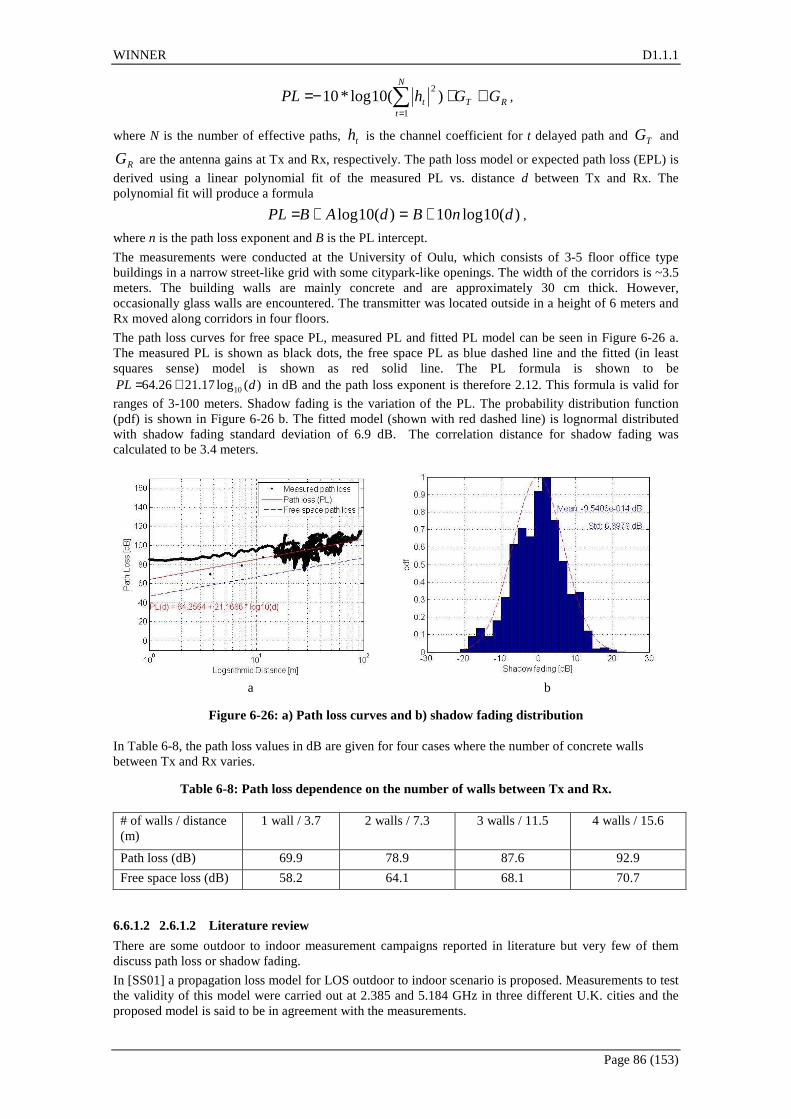
WINNER D1.1.1
Page 86 (153)
RT
N
tt GGhPL ++−= ∑
=1
2)(10log*10 ,
where N is the number of effective paths, th is the channel coefficient for t delayed path and TG and
RG are the antenna gains at Tx and Rx, respectively. The path loss model or expected path loss (EPL) is
derived using a linear polynomial fit of the measured PL vs. distance d between Tx and Rx. The polynomial fit will produce a formula
)(10log10)(10log dnBdABPL +=+= ,
where n is the path loss exponent and B is the PL intercept.
The measurements were conducted at the University of Oulu, which consists of 3-5 floor office type buildings in a narrow street-like grid with some citypark-like openings. The width of the corridors is ~3.5 meters. The building walls are mainly concrete and are approximately 30 cm thick. However, occasionally glass walls are encountered. The transmitter was located outside in a height of 6 meters and Rx moved along corridors in four floors.
The path loss curves for free space PL, measured PL and fitted PL model can be seen in Figure 6-26 a. The measured PL is shown as black dots, the free space PL as blue dashed line and the fitted (in least squares sense) model is shown as red solid line. The PL formula is shown to be
)(log17.2126.64 10 dPL += in dB and the path loss exponent is therefore 2.12. This formula is valid for
ranges of 3-100 meters. Shadow fading is the variation of the PL. The probability distribution function (pdf) is shown in Figure 6-26 b. The fitted model (shown with red dashed line) is lognormal distributed with shadow fading standard deviation of 6.9 dB. The correlation distance for shadow fading was calculated to be 3.4 meters.
a b
Figure 6-26: a) Path loss curves and b) shadow fading distribution
In Table 6-8, the path loss values in dB are given for four cases where the number of concrete walls between Tx and Rx varies.
Table 6-8: Path loss dependence on the number of walls between Tx and Rx.
# of walls / distance (m)
1 wall / 3.7 2 walls / 7.3 3 walls / 11.5 4 walls / 15.6
Path loss (dB) 69.9 78.9 87.6 92.9
Free space loss (dB) 58.2 64.1 68.1 70.7
6.6.1.2 2.6.1.2 Literature review
There are some outdoor to indoor measurement campaigns reported in literature but very few of them discuss path loss or shadow fading.
In [SS01] a propagation loss model for LOS outdoor to indoor scenario is proposed. Measurements to test the validity of this model were carried out at 2.385 and 5.184 GHz in three different U.K. cities and the proposed model is said to be in agreement with the measurements.

WINNER D1.1.1
Page 87 (153)
In [MHA+04] the measurements were performed in Kista, a part of city of Stockholm with mostly office buildings at 1947 MHz. The base station was placed at a window at the 6th floor of an office building and the mobile at 6 different locations on three different floors of another office building. The distance between them was 300 m. The average path loss measurement results are pictured in Figure 6-27. Path loss of more than 20 dB in excess of free space loss was measured even in LOS condition. This was due to heat protective window coating.
Figure 6-27: Average path loss measured at each location and array orientation. The solid line corresponds to free space loss and the dashed line to free space loss + 22dB.
In reference [CKC03] the transmitter was placed outside a building where the receiver was moving in the corridors on the first and second floors and the measurements were conducted at 2 GHz. The maximum distance between the transmitter and the receiver was 15 meters and the maximum RF output was +13 dBm. The path loss exponent was observed to be of the order -1.0 for both floors. Path loss for second floor is presented in the figure below.
Figure 6-28: Signal attenuation on the second floor at 2 GHz.
[MOT02] proposes an outdoor-to-indoor path loss model that considers the paths through wall openings. The measurements were conducted at a department store at 8.45 GHz and the transmitting antenna was at a height of 14 meters. The path loss model assumes that the loss is a sum of outdoor propagation loss, wall opening penetration loss, and indoor propagation loss. The measurements show that the penetration

WINNER D1.1.1
Page 88 (153)
loss of wall openings ranges from 5 to 28 dB with a mean value of 17.2 dB. The indoor attenuation coefficient was measured to be 0.348 dB/m.
6.6.1.3 Interpretation of the results
The results show that a concrete wall attenuates the signal approximately 9dB. This is in the range of values reported in [MOT02]. The measured path loss exponent of 2.12 is also very understandable and in line with the values reported in [WIN1D54].
6.6.2 RMS and maximum excess delay distribution
2.6.2.1 Measurement results
The measurements were conducted at the University of Oulu. The Tx was located in a lifter in a height of 6 meters, which corresponds to approximately 2nd-3rd floor in the building. The results are analyzed over several routes in different floors of the building.
In Table 6-9, the distribution of RMS delay spread is investigated in eight cases when Rx is moving in floors 1,2,3 and 4. R stands for room, C for corridor and w for window.
Table 6-9: RMS delay spread statistics in different floors and different office environments
Stat (ns)\Floor # Floor 1 Floor 2 Floor 3 Floor 4
R (w) R (large w) C (w) R (w) C (w) R (w) C (w) R (w)
Mean 139 28 50.4 27.1 78.6 25.7 48.9 46.9
Std 25.7 20 16.9 21.2 51.5 16.1 17.6 28.4
10% percentile 106.5 7.9 31.2 5 27.9 7.4 25.5 16.6
50% percentile 136.1 21.3 47.5 17.4 52.7 22.2 47.4 44.7
90% percentile 175.8 55.6 73.3 59.5 157.9 46.7 74.5 88.9
In Figure 6-29, the cumulative distribution function (cdf) of the measured RMS delay spread and its normal distribution are shown. The normal distribution applied values 64.9 ns and 42.7 ns as mean and standard deviation, respectively. The correlation distance of RMS delay spread was found to be 9.2 meters.
Figure 6-29: Cdf of RMS delay spread.

WINNER D1.1.1
Page 89 (153)
In Table 6-10, the RMS delay spread is investigated when the number of walls between the Tx and the Rx is changed from one to four. These measurements were static, i.e., the Rx did not move.
Table 6-10: RMS delay spread statistics in different floors and different office environments.
# of walls 1 wall 2 walls 3 walls 4 walls
RMS delay spread (ns) 6.8 15.0 24.9 78.6
In Table 6-11, the maximum excess delay spread distribution is shown for eight cases when Rx is moving in floors 1, 2, 3 and 4.
Table 6-11: Maximum excess delay spread statistics in different floors and different office environments
Stat (ns)\Floor # Floor 1 Floor 2 Floor 3 Floor 4
R (w) R (large w) C (w) R (w) C (w) R (w) C (w) R (w)
Mean 573.6 220.8 316.5 254.7 403.8 283 338.6 313.1
Std 41.4 188.9 146.9 226.8 192.4 204.3 143.6 292.6
10% percentile 510 60 160 50 180 60 140 30
50% percentile 600 110 260 90 430 120 300 230
90% percentile 610 510 530 550 650 550 530 940
In Figure 6-30 the cdf for maximum excess delay spread is shown together with normally distributed cdf model. The calculated mean maximum excess delay spread value is 364.8 ns and standard deviation is 196.5 ns. The correlation distance of the maximum excess delay spread was found to be 8.8 meters.
Figure 6-30: Cdf of Maximum excess delay spread.
6.6.2.1 2.6.2.2 Literature review
In [WAE+04] radio channel measurements were performed at 5.2 GHz and a signal bandwidth of 120 MHz in outdoor-to-indoor office propagation scenario in Lund University, Sweden. In the measurements the transmitter was placed on three different locations on a roof top and the receiver was in an office

WINNER D1.1.1
Page 90 (153)
building southwards from the transmitter. The receiver was either in the northern rooms which were nearest to the transmitter, in the southern rooms or in the corridor between the northern and southern rooms as pictured in Figure 6-31 [WAE+04].
Figure 6-31: Measurement location in reference [WAE+04].
The rms delay spread was about 7-10 ns for half of the cases when the receiver was located in the northern rooms. The rms delay was 12-15 ns for 50 percent of the cases when the receiver was located in the southern rooms and for the corridor about 8 to 11 ns depending on the transmitter location on the roof top. The delay spread was observed to be in the range of 5-25 ns.
In [AHY06] the rms delay spread of the channel is observed to be approximately 40 ns for half of the channel samples. The measurements were conducted at 5.25 GHz and 100 MHz bandwidth in the campus area of the university of Oulu, Finland. The transmitter was located outside a building at a height of 12 m and receiver was moving in a laboratory room on the first floor of the building at a height of 1.3 m.
In [WOT99] wideband measurements were carried out at 2.44 and 5.74 GHz in Oxford, UK for static outdoor-to-indoor scenario using dual channel vector network analyzer. The measurement bandwidth was 80 MHz. Measurement environments were categorized into urban, suburban and rural. The RMS delay spread for multipath arrivals was measured to be 37± 8, 24±20 and 19±8 ns for urban, suburban and rural environments respectively. The mean excess delay was 34±10, 22±30 and 13±8 ns for urban, suburban and rural environments respectively. When moving from urban to suburban and rural environments, the RMS and mean delay spread decreases. After grouping multipath arrivals into clusters the RMS delay spread was 21±3, 12±6 and 11±3 ns for urban, suburban and rural environments respectively.
[C02] reports measurements at 3.6-4.2 GHz band in Ministry of the Communications building, in Rome, Italy. The building is 8 floors, 25 meters high and U-shaped. The transmitter was placed on the top of the other wing of the building and the receiver was placed at seven sites inside the opposite wing. The distance between the transmitter and the receiver was 40-60 meters. Example of the obtained mean excess delay and RMS delay spread are pictured in Figure 6-32 and Figure 6-33 [C02] respectively.

WINNER D1.1.1
Page 91 (153)
Figure 6-32: Mean delay spread.
Figure 6-33: RMS delay spread.
2.6.2.3 Interpretation of the results
Measured delay spread values are relatively large compared to literature. However, delay spread calculations are highly dependant on the way the threshold level is chosen, i.e., the way we choose which delay taps are taken into account and which are not.
In our measurement analysis, the threshold was set in such a way that all the taps that are less than 20 dB below the level of the peak power, were accounted for. Furthermore, the dynamic range of a snap shot was required to be at least 23 dB in order to be accounted for in the analysis. Another option is to select those taps that are more than, for example, 3 dB above the noise level as effective taps. If this method had been applied the delay spread results would have been higher, approximately 1.3 times the values presented in Section 2.6.2.1.
6.6.3 Azimuth AS at BS and MS
6.6.3.1 Measurement results
Azimuth angle spread is calculated as described in [3GPPSCM] from DoA, DoD and path powers. It is known as circular angle spread. In the analysis results Tx is considered as the outdoor base station (BS) and Rx as the indoor mobile station (MS).
In Table 6-12, the azimuth angle spreads for different environments in four different floors are given. It can be seen that the azimuth spread values at the indoor MS are significantly higher than the ones in outdoor BS.

WINNER D1.1.1
Page 92 (153)
Table 6-12: RMS azimuth angle spread in different floors.
Floor 1 Floor 2 Floor 3 Floor 4 Stat (degrees) \ Floor # R (w) R (large w) C (w) R (w) C (w) R (w) C (w) R (w)
Mean 16.6 21.9 13.7 12.0 14.6 8.6 12.5 9.4
Std 12.1 9.4 8.9 7.1 10.8 3.4 11.3 4.8
10% 2.8 9.2 1.5 6.0 1.6 4.8 1.2 5.8
50% 16.7 21.0 13.4 10.5 13.7 8.2 9.1 7.8
Tx (Out)
90% 32.9 34.6 23.5 19.7 29.5 12.7 30.5 14.7
Mean 74.6 62.3 61.4 55.0 65.7 65.2 62.0 72.2
Std 7.1 13.5 15.6 18.8 15.0 13.5 16.0 14.3
10% 66.0 46.1 40.6 30.7 46.0 44.8 42.1 52.1
50% 74.3 60.8 62.2 52.6 65.8 67.6 61.7 76.4
Rx
(In)
90% 84.3 81.7 81.2 81.7 85.4 80.0 83.5 85.7
Corresponding values for both terminals averaged over all routes are shown in Table 6-13. The cdf curves, based on the values in Table 6-13, are shown in Figure 6-34.
Table 6-13: RMS azimuth angle spread averaged over all routes.
Stat (degrees) \ Terminal
Tx (outdoor) Rx (indoor)
Mean 17.3 60.8
Std 12.6 17.0
10% 2.9 38.1
50% 14.2 61.4
90% 36.5 82.8
CorrDist (m) 10.6 6
Figure 6-34: Cdf for RMS azimuth spread for both terminals.

WINNER D1.1.1
Page 93 (153)
6.6.3.2 Literature
In [WAE+04] angular spread and rms angular spread were reported. The measurements were performed at 5.2 GHz and bandwidth of 120 MHz in Lund University, Sweden. The transmitter was placed on a roof top [WAE+04]. The receiver was placed in the northern rooms, in the corridor and in the southern rooms. The angular spread at the indoor link was measured to be 30-55 degrees and at the outdoor link 4-20 degrees. When comparing the rms angular spreads at the receiver end (DOA), the transmitter position does not affect the rms spread or the mean angular spread. At the transmitter end (DOD) the transmitter position causes large differences in the rms spread.
[MHA+04] reports narrowband MIMO radio channel measurements in an urban macrocellular outdoor-to-indoor propagation scenario at 1947 MHz. The location of the measurements was Kista, a part of the city of Stockholm mostly containing office buildings with 5-8 storeys. The base station was placed at a large window at the 6th floor of an office building and the mobile was placed at different locations on different floors of another office building at 300 m distance of the base station. The angular spread was observed to be small due to lack of scattering (2-12 degrees).
In [WOT99] wideband measurements were carried out at 2.44 and 5.74 GHz in Oxford, UK for static outdoor-to-indoor scenario using dual channel vector network analyzer. The measurement bandwidth was 80 MHz. Measurement environments were categorized into urban, suburban and rural. The RMS azimuth spread for multipath arrivals was measured to be 89±21, 81±15 and 67±16 degrees for urban, suburban and rural environments respectively. After grouping the multipath arrivals into clusters, the RMS azimuth spread was 7.0±1.0, 8.8±1.9 and 8.4±1.5 for urban, suburban and rural environments respectively.
6.6.3.3 Interpretation of the results
The measured RMS azimuth spread results are well in line with the existing literature results.
6.6.4 Elevation AS at BS Azimuth angle spread is calculated as described in [3GPPSCM] from DoA, DoD and path powers. In Figure 6-35, the cdf for elevation angle spread is shown. The mean value 14.6 degrees and standard deviation is 10.5 degrees.
Figure 6-35: Cdf for elevation angle spread at Tx

WINNER D1.1.1
Page 94 (153)
6.6.5 Cross-polarisation ratio (XPR)
6.6.5.1 Measurement results
The cross-polarization ratio (XPR) vertical (v) is defined as the ratio of power received from vertical to vertical polarization to the power received from vertical to horizontal polarization. Respectively, XPRh is defined as the ratio between the powers of horizontal to horizontal and horizontal to vertical polarizations. In Table 6-14, XPR values averaged over all the routes are given in dB. PeakXPR denotes the peak path’s XPR values, whereas scatXPR is the XPR values for the scattered multipaths (all except the peak path). The cdfs are plotted in Figure 6-36.
Table 6-14: Cross-polarization ratios averaged over all the routes.
Stat (dB) \ Terminal
Peak XPRv Peak XPRh Scat XPRv Scat XPRh
Mean 3.99 9.54 -1.11 5.64
Std 11.21 11.31 8.87 8.76
10% -10.73 -6.04 -11.84 -5.18
50% 4.14 11.23 -1.43 5.71
90% 17.96 22.38 10.11 16.24
Figure 6-36: Cdfs for cross-polarizations ratios (XPR).
6.6.5.2 Interpretation of the results
The results are well in line with the results in [WIN1D54]. Furthermore, the results show that polarization change from horizontal to vertical involves more power loss than a change from vertical to horizontal.
6.6.6 Power Delay Profile
6.6.6.1 Measurement results
Power delay profile (PDP) is the distribution of the powers of the multipath components versus the delay. Typical PDP in an outdoor to indoor environment is shown in Figure 6-37. The PDPs are fitted to exponential function
btetPDP −=)( ,
where t is the multipath delay and b is the time constant.

WINNER D1.1.1
Page 95 (153)
Figure 6-37: Typical power delay profile.
6.6.6.2 Interpretation of the results
Typical PDP curve is very reasonable. In indoor environment, the receiver is likely to receive multiple relatively strong multipaths.
6.6.7 Proportionality factors, delay and angular
6.6.7.1 Measurement results
The delay proportionality factor is defined as the ratio between the standard deviation of the delays of the multipath components and RMS delay spread. In Table 6-15, the mean, standard deviation and the percentiles for 10%, 50% and 90% of the cdf for the delay proportionality factor in outdoor-to-indoor environment is shown. Four different floors are investigated with two different cases (corridor and office room).
Table 6-15: Delay proportionality factor in different floors.
Stat \ Floor # Floor 1 Floor 2 Floor 3 Floor 4
R (w) R (large w) C (w) R (w) C (w) R (w) C (w) R (w)
Mean 1.23 2.21 1.65 2.43 1.61 2.34 1.83 2.14
Std 0.21 0.70 0.31 0.57 0.33 0.57 0.23 0.78
10% percentile 0.97 1.46 1.38 1.63 1.19 1.64 1.54 1.29
50% percentile 1.21 2.05 1.58 2.43 1.59 2.24 1.82 1.97
90% percentile 1.53 3.17 1.98 3.18 2.07 3.10 2.15 3.41
In Figure 6-38, the cdf of the measured delay proportionality factor averaged over all the routes is given. The mean value is 1.77 and the standard deviation (std) is 0.53. The red dashed line is the fitted normally distributed cdf with above mentioned mean and std values.

WINNER D1.1.1
Page 96 (153)
Figure 6-38: Cdf for RMS delay spread proportionality factor.
The angular proportionality factor is defined as the ratio between the standard deviation of the azimuth angles of the multipath components and the RMS angular spread. The measured azimuth angular proportionality factors are shown in Table 6-16 for different floors. In Figure 6-39, the cdf of the measured azimuth angular proportionality factor averaged over all the routes is given for both terminals. The mean and the standard deviation (std) values are given in Table 6-17.
Table 6-16: Angular proportionality factor in diff erent floors.
Floor 1 Floor 2 Floor 3 Floor 4 Stat \ Floor #
R (w) R (large w) C (w) R (w) C (w) R (w) C (w) R (w)
Mean 1.28 1.12 1.14 1.23 1.05 1.20 1.09 1.16
Std 0.50 0.34 0.39 0.34 0.38 0.23 0.42 0.25
10% 0.75 0.76 0.68 0.76 0.56 0.89 0.61 0.87
50% 1.16 1.07 1.09 1.21 1.05 1.21 1.07 1.13
Tx (Out)
90% 1.96 1.55 1.62 1.67 1.56 1.49 1.59 1.50
Mean 1.43 1.63 1.60 2.16 1.49 1.69 1.56 1.51
Std 0.14 0.32 0.61 0.87 0.49 0.45 0.68 0.36
10% 1.26 1.30 1.08 1.31 1.06 1.29 1.05 1.21
50% 1.41 1.59 1.42 1.99 1.34 1.55 1.33 1.40
Rx
(In)
90% 1.60 2.05 2.30 1.67 2.12 2.18 2.34 1.88
Table 6-17: Angular proportionality factor statisti cs for both terminals.
Stat \ Terminal Tx (outdoor) Rx (indoor)
Mean 1.20 1.69
Std 0.39 0.80
10% 0.76 1.09
50% 1.14 1.47
90% 1.67 2.54

WINNER D1.1.1
Page 97 (153)
Figure 6-39: Cdf for RMS angular spread proportionality factor at Tx and Rx ends.
In Figure 6-40, the proportionality factor for elevation angle spread is shown for Tx end. The mean and std values are 1.16 and 0.4, respectively.
Figure 6-40: Proportionality factor for elevation angle spread at Tx.
6.6.7.2 Interpretation of the results
The measured delay proportionality values were well inline with the values presented for similar scenarios such as A1 in [WIN1D54].

WINNER D1.1.1
Page 98 (153)
6.6.8 Main DoA and DoD offset
6.6.8.1 Measurement results
Main DoA and DoD angles are defined as the difference between the LoS direction and the mean angle of the angles of the effective multipaths. In outdoor case this difference is relatively small. However in indoor terminal, the values can vary significantly as shown in Table 6-18 and Table 6-19. The cdfs of main azimuth angle offset for both terminals are presented in Figure 6-41.
Table 6-18: Main azimuth angle direction offset compared to LoS path in different floors.
Floor 1 Floor 2 Floor 3 Floor 4 Stat (degrees) \ Floor # R (w) R (large w) C (w) R (w) C (w) R (w) C (w) R (w)
Mean 7.2 2.6 -7.0 -12.6 -4.9 -11.6 -8.0 -17.5
Std 12.9 8.6 7.1 4.1 6.4 3.2 6.3 13.3
10% -3.8 -8.7 -15.6 -18.6 -13.7 -16.0 -15.5 -35.4
50% 2.2 2.7 -7.5 -11.8 -4.3 -10.6 -9.1 -12.3
Tx (Out)
90% 31.1 13.0 2.5 -8.0 2.6 -8.4 1.6 -1.5
Mean 3.7 -17.5 47.1 -7.7 51.8 -13.7 42.8 15.3
Std 137.3 90.8 62.0 87.5 62.9 85.4 63.4 103.8
10% -158.4 -107.5 -33.9 -116.3 -22.4 -125.9 -39.6 -98.9
50% -66.4 -52.4 49.2 -13.2 50.9 -4.7 43.6 4.1
Rx
(In)
90% 164.1 145.6 127.5 125.9 135.7 94.6 127.9 156.4
Table 6-19: Main azimuth angle direction offset compared to LoS path averaged over all routes.
Stat (degrees) \ Terminal
Tx (outdoor) Rx (indoor)
Mean 0.5 -17.6
Std 18.7 97.9
10% -18.2 -139.4
50% -1.9 -32.5
90% 22.2 128.4

WINNER D1.1.1
Page 99 (153)
Figure 6-41: Cdf for main DoA and DoD azimuth offset.
In Figure 6-42, the pdf for the azimuth angles at Tx (outdoor) terminal is shown. The red dashed line is the normally distributed pdf fitted to the data. The corresponding figure for elevation angles is presented in Figure 6-43.
Figure 6-42: Pdf for DoDs in azimuth domain for BS (outdoor).

WINNER D1.1.1
Page 100 (153)
Figure 6-43: Pdf for DoDs in elevation domain for BS (outdoor)
6.6.8.2 Interpretation of the results
The fact that outdoor transmitter (BS) has significantly lower main angular offsets than the indoor MS is very reasonable. In indoor environment, the receiver is close to several walls and equipments that are likely to produce some reflections.
6.6.9 Ricean K-factor
6.6.9.1 Measurement results
Ricean K-factor is the ratio of the dominant path power to the power of the diffused paths. On the other hand, Ricean K-factor can be used to describe the stability of the dominant path’s power as the Rx moves along the route. This method is applied here and the results are shown in dB in the tables below.
In Table 6-20, the statistics of K-factor cdf in different floors are shown. Also the indoor environment type is investigated in terms of corridor and office room. The observation interval was chosen to be 0.75 meter which corresponds to approximately 13 wavelengths.
Table 6-20: K-factor statistics in different floors and different office environments
Stat (dB) \ Floor # Floor 1 Floor 2 Floor 3 Floor 4
R (w) R (large w) C (w) R (w) C (w) R (w) C (w) R (w)
Mean 6.70 8.00 5.84 9.32 6.53 8.99 7.14 10.11
Std 2.98 3.72 3.33 4.06 2.87 3.63 3.57 5.38
10% percentile 2.86 3.32 2.70 4.64 3.00 4.46 3.23 4.14
50% percentile 6.62 8.04 6.08 9.38 6.73 8.86 7.65 9.85
90% percentile 10.47 12.60 9.12 14.24 9.91 13.75 10.78 17.37
In Figure 6-44, the cdf for the averaged K-factor over all the analysis routes is shown together with its statistics and normally distributed cdf model. In addition, the K-factor (KF) formula was calculated to be
dKF *001.0072.8 −= , where d is the distance.
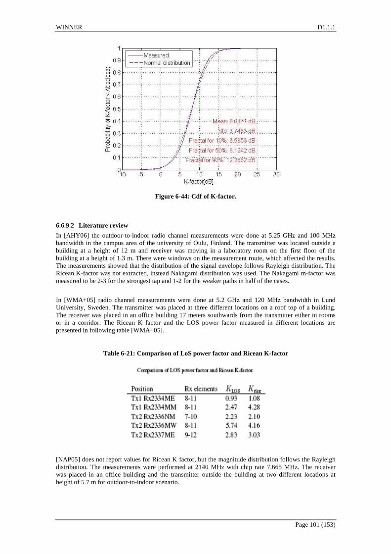
WINNER D1.1.1
Page 101 (153)
Figure 6-44: Cdf of K-factor.
6.6.9.2 Literature review
In [AHY06] the outdoor-to-indoor radio channel measurements were done at 5.25 GHz and 100 MHz bandwidth in the campus area of the university of Oulu, Finland. The transmitter was located outside a building at a height of 12 m and receiver was moving in a laboratory room on the first floor of the building at a height of 1.3 m. There were windows on the measurement route, which affected the results. The measurements showed that the distribution of the signal envelope follows Rayleigh distribution. The Ricean K-factor was not extracted, instead Nakagami distribution was used. The Nakagami m-factor was measured to be 2-3 for the strongest tap and 1-2 for the weaker paths in half of the cases.
In [WMA+05] radio channel measurements were done at 5.2 GHz and 120 MHz bandwidth in Lund University, Sweden. The transmitter was placed at three different locations on a roof top of a building. The receiver was placed in an office building 17 meters southwards from the transmitter either in rooms or in a corridor. The Ricean K factor and the LOS power factor measured in different locations are presented in following table [WMA+05].
Table 6-21: Comparison of LoS power factor and Ricean K-factor
[NAP05] does not report values for Ricean K factor, but the magnitude distribution follows the Rayleigh distribution. The measurements were performed at 2140 MHz with chip rate 7.665 MHz. The receiver was placed in an office building and the transmitter outside the building at two different locations at height of 5.7 m for outdoor-to-indoor scenario.

WINNER D1.1.1
Page 102 (153)
In [CKC03] the transmitter was placed outside a building where the receiver was moving in the corridors on the first and second floors and the measurements were conducted at 2 GHz with the maximum RF output being +13 dBm. The maximum distance between the transmitter and the receiver was 15 meters. The Ricean K-factor was observed to be 21.3 and 18.7 for the first and second floors respectively.
Reference [SMJ+99] presents measurements at 2.44 GHz and 80 MHz span with 3 different transmitter sites and the receiver located in a room. The transmit power was 20 dBm and the measurements were conducted with dual channel VNA-based wideband channel measurement system. The Ricean K-factor was observed to have a very large variability on both channels.
6.6.9.3 Interpretation of the results
The measured K-factor values are well in range with the values encountered in literature review. However, in [AHY06] and in [WMA+05] the observed values are smaller. In our measurements, a transmit power of 26 dBm was applied, the height of the Tx was 6 meters and the distance between Tx and Rx was relatively short. In this light, the increase of the Ricean K-factor values compared to [AHY06] and in [WMA+05] is understandable.
6.6.10 Cross-Correlations
6.6.10.1 Measurement results
In Table 6-22, the cross-correlation coefficients for different parameters are given. Logarithmic RMS (LogRMS) delay spread versus shadow fading is shown in Figure 6-45.
Table 6-22: Cross-correlation coefficients between parameters
Parameters Cross-correlation coefficient
AoD vs. SF -0.30
AoA vs. SF 0.04
AoD vs. RMS DS 0.26
AoA vs. RMS DS -0.0006
AoA vs. AoD -0.13
SF vs. logDS 0.47
Figure 6-45: Correlation between logarithmic RMS delay spread and shadow fading.
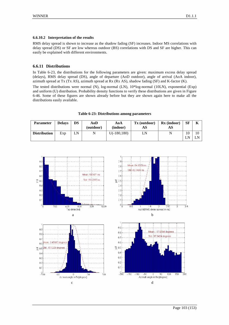
WINNER D1.1.1
Page 103 (153)
6.6.10.2 Interpretation of the results
RMS delay spread is shown to increase as the shadow fading (SF) increases. Indoor MS correlations with delay spread (DS) or SF are low whereas outdoor (BS) correlations with DS and SF are higher. This can easily be explained with different environments.
6.6.11 Distributions In Table 6-23, the distributions for the following parameters are given: maximum excess delay spread (delays), RMS delay spread (DS), angle of departure (AoD outdoor), angle of arrival (AoA indoor), azimuth spread at Tx (Tx AS), azimuth spread at Rx (Rx AS), shadow fading (SF) and K-factor (K).
The tested distributions were normal (N), log-normal (LN), 10*log-normal (10LN), exponential (Exp) and uniform (U) distribution. Probability density functions to verify these distributions are given in Figure 6-46. Some of these figures are shown already before but they are shown again here to make all the distributions easily available.
Table 6-23: Distributions among parameters
Parameter Delays DS AoD (outdoor)
AoA (indoor)
Tx (outdoor) AS
Rx (indoor) AS
SF K
Distribution Exp LN N U(-180,180) LN N 10LN
10LN
a b
c d

WINNER D1.1.1
Page 104 (153)
e f
g h
Figure 6-46: Distributions among the following parameters: a) maximum excess delay spread, b) RMS delay spread, c) AoD, d) AoA, e) Tx azimuth spread, f) Rx aximuth spread, g) shadow fading
and h) Ricean K-factor.
6.6.12 Outdoor-to-indoor results by CU/CRC CRC conducted outdoor-to-indoor measurements in a 100 MHz bandwidth centred at 4.95 GHz. The transmitter was housed in a large van, parked in front of a 4-story brick building, on the broad (windowed) side of the building.
6.6.12.1 Propagation Loss
Excess transmission losses were estimated in a similar manner to work reported in [deJKH02] by evaluating the sum of the squares of the values in Average Power Delay Profiles (APDPs) for each measurement run, comparison against a calibration reference, and appropriately accounting for free space loss and measurement system gains and losses. Excess loss varied from floor-to-floor and depending on whether the Rx was on the illuminated or back side of the building or in the hallway. In summary, such losses varied from 20-50 dB in the basement, 10-30 dB on the ground floor, 7-27 dB on the second floor, and from 7-32 dB on the third (top) floor.
6.6.12.2 Rms Delay Spreads
Values for rms delay spread also varied with measurement location, but their minimum and maximum values were about the same on all floors, being 9 ns and 30 ns, respectively. The median values were about 16 ns, except on the second floor, where the median was 21 ns. The reason for the higher values on the second floor is not clear at the time of writing. Figure 6-47, shows an experimentally determined cumulative probability distribution function (ECDF) for rms delay spreads from all measurement locations in the building. For values estimated using a 20 dB threshold, the figure shows a median of 19 ns, with maximum and minimum values of 8 and 29 ns, respectively.

WINNER D1.1.1
Page 105 (153)
Figure 6-47: ECDF of rms delay spreads computed from data recorded in all measurement locations, on all floors.
6.6.12.3 Narrowband envelope fading
Equivalent CW envelope fading distributions were estimated, as outlined in [RJB89], from the variations in single spectral lines in measured channel transfer function time series from all measurement locations in the building. Figure below is an ECDF of the results.
−2 0 2 4 6 8 10 120
0.1
0.2
0.3
0.4
0.5
0.6
0.7
0.8
0.9
1Rician K Ratios for Non−Rayleigh Cases (dB)−(All Floors)
Pro
b[K
(dB
).LE
.Abs
ciss
a]
10*log10(Random Power/Coherent Power)=K (dB)
16/72 Files exhibited Rayleigh Fading
Figure 6-48: ECDFs for K ratios on Rician channels on all floors in the building.
The text in the figure explains that Rayleigh fading was exhibited in only 16 of the 72 measurement locations. Fading in the other locations exhibited Rician Characteristics, with K ratios that ranged from –1 dB to + 11 dB. In the Rayleigh cases, coherence bandwidths would be approximately equal to the reciprocal of rms delay spreads. The minimum would therefore be about 1/(30 ns) or 33 MHz. Such bandwidths are already extremely large, but would be greater on the Rician channels [RJB02], where the reciprocal rms delay spread-coherence bandwidth relationship does not apply.
5 10 15 20 25 300
0.1
0.2
0.3
0.4
0.5
0.6
0.7
0.8
0.9
1rms Delay Spreads (All Floors)
Pro
b[rm
s D
elay
Spe
ad .L
E. a
bsci
ssa]
rms Delay Spread (ns)
Threshold=20 dB
Threshold=30 dB
Threshold=40 dB

WINNER D1.1.1
Page 106 (153)
6.6.13 Combined results Results reported by UOULU and CRC are different for several reasons. The main reason is the differences in building characteristics. Due to the fact that UOULU is located in Europe and CRC in North-America, the building materials and dimensions deviate from each other significantly. This is bound to result in different analysis conclusions. Other minor reasons for deviations could include the sounder characteristics and applied settings, the antenna characteristics, the methods used to move the receive antenna during the measurements, as well as the distances over which it was moved corresponding to individual results. Although attempts were made to make analysis procedures the same, there were peculiarities of the recorded data that made some data preprocessing differences necessary.
Since the UOULU data set is more complete, with corresponding AoA information, and the analysis procedures section of this report is more closely aligned with analyses conducted at UOULU, the UOULU results were chosen for reporting in the generic channel model table, Table 4-5. The CRC results are left, however, for examination in this section, as comparison of these with the UOULU results is a good example of how results reported in the literature can vary, and, as discussed in the opening sentence of this paragraph, why such variations can occur.
6.7 B5 – Stationary Feeder
There are five sub-scenarios for the Stationary Feeder, B5a – B5d and B5f. In this document only sun-scenarios B5a, B5c and B5f are discussed, because those are the ones requested by the other Tasks of WINNER2. The interested reader may consult [WIN1D54] about B5b and B5d.
6.7.1 B5a– Fixed Stationary Feeder: Roof-top to Roof-top (LOS) The scenario definition for B5a LOS Fixed Relay, rooftop to rooftop, is given in [D5.4]. The channel model is taken as such from the [WIN1D54], because the frequency dependence was included in the model. On the other hand the connection is almost like in free space, so that the path-loss does not depend noticeably on the antenna heights. The equation is given in slightly different form to comply with the other equations. The path-loss is
PL(d, f) = 23.5 log10 (d) + 42.5 + 20 log10 (f [GHz]/5.0), σ = 3.4 dB (6.21)
where d = distance
f = center frequency
σ = standard deviation of the shadow fading.
The path-loss curves for frequencies 2 to 5 GHz can be seen in the Figure 6-49.

WINNER D1.1.1
Page 107 (153)
Figure 6-49. B5a Fixed stationary feeder (rooftop to rooftop) subscenario path-loss curves for the frequencies between 2 and 5 GHz.
6.7.2 B5c – Fixed Stationary Feeder: Below Roof-top to Street Level The sub-scenario B5c has been described in [WIN2IR111]. The connection is from a height somewhat below roof-top level to a Fixed Relay Station (FRS) with height 3 – 5 m. Here we assume that the BS antenna height is 15 m and Relay height is 3 to 5 m and there is a LOS connection between the BS and FRS. The BS to FRS connection can be modelled with the B1 channel model, taking into account that the FRS is stable. Path-loss model is then
PL(d1, f) = 22.7 log10 (d1 [m]) + 41.0 + 20 log10(f [GHz]/5)), 30m <= d1 <= d’BP (6.22)
σ = 3.0 dB
PL(d1, f) = 40.0 log10 (d1 [m]) + 9.45 - 17.3log10 (h’BS [m]) - 17.3log10 (h’MS [m]) + (6.23)
2.7log10(f [GHz]/5.0), d > d’BP
σ = 6.0 dB
The break-point is calculated with
d’BP = 4 · h’BS·h’RS· f /c
where h’BS = effective antenna height of the base station (real height – 1.5 m assumed).
h’RS = effective antenna height of the relay station, (real height – 1.5 m assumed).
f = centre-frequency (Hz)
c = velocity of light in vacuum
The height gain factor in (13b) has to be restricted to values giving loss greater than equation (13a). In the formula it has been assumed that the effective antenna height is the real height minus 1.5m, the assumed mean vehicle height on the street.
The FRS to MS connection can also be modelled with the B1 channel model. Now the FRS antenna height is limited to 3 to 5 m. In other respects the situation is identical to the ordinary B1 case.

WINNER D1.1.1
Page 108 (153)
Figure 6-50. B5c LOS path-loss at 2 to 5 GHz compared to the 2 GHz free-space path-loss.
The path-loss of the B5c LOS model is smaller than free space loss, when the distance is less than 100 m. This situation must be prevented by restricting the path-loss always to be higher than or as high as the free-space loss.
6.7.3 B5f – Fixed Stationary Feeder: Roof-top to Roof-top (NLOS) The scenario definition for B5f NLOS Fixed Relay, rooftop to rooftop, has been given first in [WIN2IR6.13.3]. Below we specify the scenario in more detail. We must also point out that the model specified below has to be refined later. At the moment the model is based totally on existing literature.
6.7.3.1 Scenario definition
The scenario for the NLOS Fixed Relay is shown in the Figure 6-51. The Relay Station is shadowed due to some obstacle. The proposed model is formed from the B5a LOS Fixed Relay model by attenuating artificially its direct component by 15 dB in average and summing to it a normally distributed random decibel number with standard deviation 8 dB.
Feeder-link B5f
Master-station
MS
Relay
Relay to MS: B1
Figure 6-51. NLOS Fixed Relay.

WINNER D1.1.1
Page 109 (153)
6.7.3.2 Path-loss formula
Path-loss for the B5f scenario is given below
PL(d, f) = 23.5 log10 (d) + 57.5 + 20 log10 (f [GHz]/5.0), σ = 8 dB ((6.24)
where the notation is the same as used in the previous equations.
The formula is based on the references [ZEA99] and [GEA03]. We emphasize that the model is just
indicative. It is assumed to work in the distance range 0.2 to 1 km with the default antenna heights.
Figure 6-52. B5f Fixed stationary feeder (rooftop to rooftop, NLOS) subscenario path-loss curves for the frequencies between 2 and 5 GHz.
6.7.3.3 B5f model parameters
The other model parameters than path-loss are the same as in B5a, except that the strength of the first tap is decreased 15 dB and the tap powers normalized after that.
6.8 C1 – Suburban macro-cell
Measurements for the suburban C1 LOS scenario were conducted at the centre-frequency 5.25 GHz. Measurements were performed in Heinäpää relatively near to Oulu centre in an area, where the houses are lower than in the centre of the town, with some parking lots, parks and trees along the streets in between the houses. The height of the houses varied typically from 3 to 6 stories. In this document only path-loss for the C1 LOS is considered. All other channel parameters are documented in [WIN1D54].
Measurements for C1 NLOS scenario were made at 5.3 GHz in Helsinki suburban residential areas. The parameters proposed for C2 WINNER II model are not solely from those measurements, but also results from literature have been used for model parameter design.

WINNER D1.1.1
Page 110 (153)
6.8.1 Path loss and shadow fading
6.8.1.1 LOS case
In [WIN1D54] the LOS path-loss was given at 5.25 GHz as
PL(d) = 41.6 + 23.8 log10(d) 20 m < d <= dBP (6.25)
= 41.6 + 40 log10(d / dBP) + 23.8 log10(dBP) d1 >= dBP (6.26)
σ = 4.0 dB, 20 m < d <= dBP ; σ = 6.0 dB, d > dBP
Extended to 2 – 6 GHz the path-loss formula can be presented as follows:
PL(d,f) = 41.2 + 23.8 log10(d) + 20 log10(f [GHz]/5), 20 m < d <= dBP (6.27)
PL(d,f) = 40.0 log10 (d1 [m]) + 11.65 - 16.2log10 (hBS [m]) - 16.2log10 (hMS [m]) + (6.28)
3.8log10(f [GHz]/5.0), d > dBP
σ = 4.0 dB, 20 m < d <= dBP ; σ = 6.0 dB, d > dBP
where d = distance
dBP = 4 · hBS·hMS· fc /c
hBS = the height of the base station
hMS = the height of the mobile station
f = the centre-frequency (Hz)
c = the velocity of light in vacuum
σ = standard deviation.
The height gain factor in (15b) has to be restricted to values giving loss greater than equation (15a). In the formula it has been assumed that the effective antenna height is the real height, because in suburban areas it is assumed that the vehicle density is relatively small.
6.8.1.2 NLOS case
Propagation studies at 5 GHz frequency band in indoor domestic, office and commercial environments have been frequently reported, but wideband outdoor studies at 5 GHz are not as numerous. In [ZKV+02] results for urban, suburban and rural environments have been reported. In this case the maximum mobile (MS) to base station (BS) distances were limited up to 300 meters, which for outdoor cellular channel modeling is not fully representative. Path loss models around 5 GHz in residential areas and with BS heights less than 10 meters are reported in [SG00] and [DRX98].
More studies around 2 GHz frequency have been made. In [EGT+99] results for extensive macrocellular suburban measurements in US have been reported with BS antenna heights 12…79 meters. Maximum MS-BS distances up to 8 kms were measured in variety of environments containing both hilly and flat terrains as well as light and moderate-to-heavy tree densities. Shadow fading standard deviation was found to be in range 5-16 dB, and path loss exponent was always found to be greater than two. Path loss exponent was found to have a strong dependency on the BS antenna height and the terrain type: the higher the BS antenna height the smaller the path loss exponent.
In [MRA93] and [MEJ91] radio propagation differences between 900 and 1800 MHz carrier frequencies have been compared in different environments. In both the studies it was found that path loss values at 900 and 1800 MHz were highly correlated, and there was no significant difference in distance dependent behaviour. Theoretical free space path loss difference between 900 and 1800 MHz is 6 dB, and in flat open areas a value very close to it, 5.7 dB, was obtained [MRA93]. In suburban areas, however, this difference was increased to 9.3 dB [MRA93], which was explained to be due to higher vegetation in suburban environments, which attenuate 1800 MHz signals more than 900 MHz signals. In [MRA93] PL differences between 900 and 1800 MHz frequencies were found to be 9…11 dB, i.e. higher than theoretical free space loss. In [MEJ91] shadow fading standard deviation was found to be approximately 1 dB higher at 1800 MHz, which agrees with results from Okumura [OOK+68].
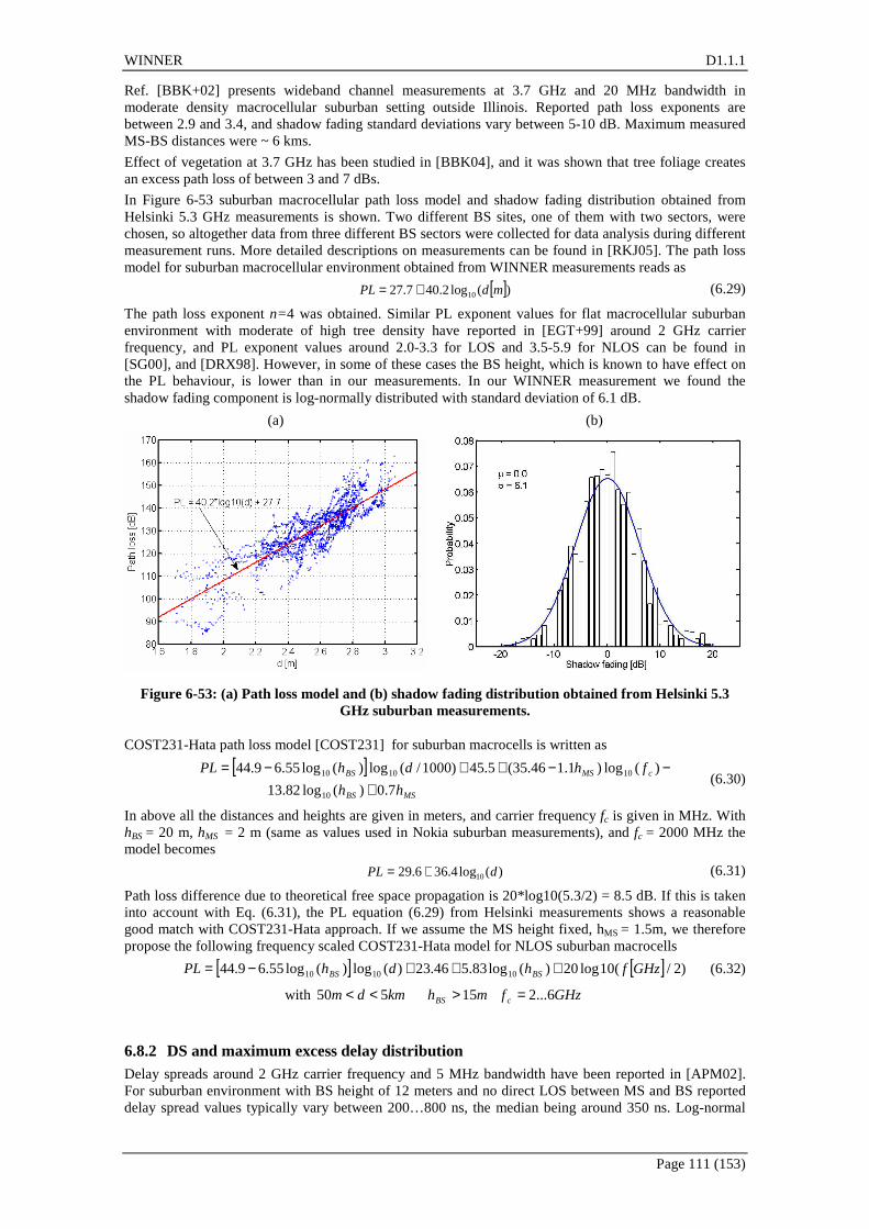
WINNER D1.1.1
Page 111 (153)
Ref. [BBK+02] presents wideband channel measurements at 3.7 GHz and 20 MHz bandwidth in moderate density macrocellular suburban setting outside Illinois. Reported path loss exponents are between 2.9 and 3.4, and shadow fading standard deviations vary between 5-10 dB. Maximum measured MS-BS distances were ~ 6 kms.
Effect of vegetation at 3.7 GHz has been studied in [BBK04], and it was shown that tree foliage creates an excess path loss of between 3 and 7 dBs.
In Figure 6-53 suburban macrocellular path loss model and shadow fading distribution obtained from Helsinki 5.3 GHz measurements is shown. Two different BS sites, one of them with two sectors, were chosen, so altogether data from three different BS sectors were collected for data analysis during different measurement runs. More detailed descriptions on measurements can be found in [RKJ05]. The path loss model for suburban macrocellular environment obtained from WINNER measurements reads as
[ ])(log2.407.27 10 mdPL += (6.29)
The path loss exponent n=4 was obtained. Similar PL exponent values for flat macrocellular suburban environment with moderate of high tree density have reported in [EGT+99] around 2 GHz carrier frequency, and PL exponent values around 2.0-3.3 for LOS and 3.5-5.9 for NLOS can be found in [SG00], and [DRX98]. However, in some of these cases the BS height, which is known to have effect on the PL behaviour, is lower than in our measurements. In our WINNER measurement we found the shadow fading component is log-normally distributed with standard deviation of 6.1 dB.
(a)
(b)
Figure 6-53: (a) Path loss model and (b) shadow fading distribution obtained from Helsinki 5.3 GHz suburban measurements.
COST231-Hata path loss model [COST231] for suburban macrocells is written as
[ ]
MSBS
cMSBS
hh
fhdhPL
7.0)(log82.13
)(log)1.146.35(5.45)1000/(log)(log55.69.44
10
101010
+−−++−=
(6.30)
In above all the distances and heights are given in meters, and carrier frequency fc is given in MHz. With hBS = 20 m, hMS = 2 m (same as values used in Nokia suburban measurements), and fc = 2000 MHz the model becomes
)(log4.366.29 10 dPL += (6.31)
Path loss difference due to theoretical free space propagation is 20*log10(5.3/2) = 8.5 dB. If this is taken into account with Eq. (6.31), the PL equation (6.29) from Helsinki measurements shows a reasonable good match with COST231-Hata approach. If we assume the MS height fixed, hMS = 1.5m, we therefore propose the following frequency scaled COST231-Hata model for NLOS suburban macrocells
[ ] [ ] )2/(10log20)(log83.546.23)(log)(log55.69.44 101010 GHzfhdhPL BSBS +++−= (6.32)
with GHzfmhkmdm cBS 6...215550 =><<
6.8.2 DS and maximum excess delay distribution Delay spreads around 2 GHz carrier frequency and 5 MHz bandwidth have been reported in [APM02]. For suburban environment with BS height of 12 meters and no direct LOS between MS and BS reported delay spread values typically vary between 200…800 ns, the median being around 350 ns. Log-normal

WINNER D1.1.1
Page 112 (153)
distribution was found to give a good fit to the measured delay spread distribution. In typical urban environments delay spreads were found to decrease with increasing BS antenna height.
In [WHL+93] rms delay spread distributions were compared in different environments at 900 MHz and 1900 MHz carrier frequencies. With both frequencies the used chip rate was 10 MHz, and data was recorded simultaneously with both the frequencies. It was seen that propagation behaviour in terms of rms delay spread was very similar with both the carrier frequencies in semirural, suburban and urban cells.
Delay spread characteristics for 3.7 GHz carrier frequency with 20 MHz bandwidth are given [KKM02]. Measurements were made in suburban areas outside Chicago, where also some distant high-rise buildings were in the environment. BS height was 49 meters, and MS was installed at 2.7 meters above the ground. 15 dB dynamics criterion from the max peak power was used in calculating delay spreads. Median delay spread values for LOS and NLOS propagation conditions were 240 and 360 ns, respectively. The combined delay spread was found to be 300 ns. As for number of rays, defined as local maxima of (instantaneous) power delay profiles, 90 percentile value of the cdf for LOS, NLOS and combined data were 3, 8 and 7 rays, respectively.
In our WINNER measurements typical delay spreads were of the order of 13…125 ns, which are considerably smaller values than reported by [APM02]. One reasons for the difference is the higher BS antenna position. Rms delay spreads have often been reported to show log-normal distribution, as summarized for example in [GEY97]. Delay spread also depends on used bandwidth due to finite system impulse size. This is discussed in more detail in section 6.9.2.
(a)
(b)
Figure 6-54: (a) Rms delay spread, and (b) maximum excess delay cdfs for Helsinki suburban macrocellular measurements at 5.3 GHz.
6.8.3 Azimuth AS at BS and MS Azimuth spreads at BS have been given in [Paj03] for rural and suburban environments at 2 GHz carrier and 10 MHz bandwidth. The mean angular spread of 2 degrees was found, with standard deviation of 2 degrees. In urban areas they have been reported to be 14 degrees and 5 degrees, respectively. The difference between the geometrical direction of the mobile and the direction of maximum received power was modelled as Gaussian. The standard deviation is about 16 degrees near the base station and decreased to 8 degrees far away in urban environment. In rural and suburban is much smaller, 2.7 degrees when distance is below 2 kms and above this decreases to 1.7 degrees. Mobile azimuth spreads were reported as 35 degrees in suburban, and 20 degrees in rural environment.
6.9 C2 – Urban macro-cell
Measurements for C2 scenario were made at 5.3 GHz in Helsinki city center. The parameters proposed for C2 WINNER II model are not solely from those measurements, but also results from literature have been used for model parameter design.
6.9.1 Path-loss and shadow fading The few reported outdoor PL measurements around 5 GHz frequency range show that typical PL exponents in urban LOS areas are close to free space propagation exponent 2, and for NLOS the reported

WINNER D1.1.1
Page 113 (153)
values vary between 3.5 and 5.8 [YMI+04][ZKV+02][Pap05]. In these cases the maximum MS-BS distances have been < 1000 meters.
Path losses and delay spreads between 430 and 5750 MHz frequencies have been compared in [Pap05]. Data was collected simultaneously at the same measurement points in multiple environments, and the chip rate at each carrier frequency was 100 MHz. Measurements were made in urban environment in Denver, which covered a combination of urban high-rise, urban low-rise and line-of sight propagation paths. BS was installed on top of a five floor building at 17 meters, and maximum measured distances in the case were up to 5 kilometers. It was observed that in line-of sight conditions close to the BS (100…300 meters) the path loss exponent was close to 2. In regions where radio paths become obstructed the path loss exponents were increasing, and they also showed frequency dependency: path loss exponent increased from 4.3 to 5.4 between 430 and 5750 MHz. The shadow fading was normally distributed, and ranged between 3 and 6 dB.
In [MRA93] and [MEJ91] radio propagation differences between 900 and 1800 MHz carrier frequencies have been compared in different environments. In both the studies it was found that path loss values at 900 and 1800 MHz were highly correlated, and there was no significant difference in distance dependent behaviour.
Path loss and delay spread results from Japanese urban metropolitan environment at 3 GHz, 8 GHz and 15 GHz frequencies are reported in [OTT+01]. The average building heights in were 20…30 meters, and BS height both clearly above (macrocell) and at rooftop level (microcell) were measured. In the measurements power delay profiles were recorded simultaneously for each of the three frequencies. Shadow fading standard deviations did not show considerable differences between frequencies, but values in the range 5…10 dB were obtained. Path loss frequency dependency was found to directly follow free space characteristics, i.e. 20log10(f). Path loss exponents were not reported.
WINNER deliverable D5.4 from phase I gives path loss models for different scenarios at 5 GHz carrier frequency for selected (fixed) base station heights. Model extensions are needed to upgrade the models for wider range of bandwidths 2-6 GHz and different BS heights. Since limited set of measurements are available in WINNER for model extensions, results found in literature has been used as a basis for the work.
6.9.1.1 Extension to different BS heights and frequency range
There are studies and channel models which address the changes in path loss due to BS height variations [KI04][COST231][EGT+99]. COST231-Hata model [COST231] for urban (metropolitan) macrocells reads as
[ ]
MSBS
cMSBS
hh
fhdhPL
7.0)(log82.13
)(log)1.146.35(5.48)1000/(log)(log55.69.44
10
101010
+−−++−=
(6.33)
Increasing the BS height has therefore a twofold effect: the propagation exponent decreases, and there the constant intercept1 changes due the BS height variation.
Similar dependencies are found in [KI04][KI04], which gives a PL formula for distances 100-1000 m, frequencies 0.4-8 GHz and BS antenna heights 30-120 m in urban areas in Japan (“Kitao”):
[ ] 2.50)(log4.20)(log9.27)(log)(log5.212.80 10101010 ++−−= fhdhPL BSBS (6.34)
In [EGT+99] the path loss model for suburban macrocells is expressed as (“Ergec”)
sddAPL ++= )/(log10 010γ (6.35)
A is a constant intercept value by a free space propagation at 100 m reference distance, and s is shadow fading component. The propagation exponent γ is a Gaussian random variable, which is written as
mhmxhcbha BSBSBS 8010,)/( ≥≥++−= γσγ (6.36)
In above the term in parenthesis is the mean of γ, x is a zero-mean Gaussian variable and σγ is the std of γ. Constants a,b,c and σγ are derived from data. For flat environment with light tree density the parameters for mean propagation exponent are a=3.6, b=0.0050 and c = 20.0.
Figure 6-55 shows the propagation exponent as a function of BS height from different models and publications [KI04][COST231][EGT+99]. Circles refer to unpublished 5.3 GHz measurements made by Nokia in Helsinki. In those measurements path loss was measured from one BS site in Helsinki city center with different BS heights (below, at and above rooftops, i.e. 18 m, 28 m and 38 m, respectively).
1 If PL model is written in form PL = A+10*n*log10(d), A is the intercept and n propagation exponent.

WINNER D1.1.1
Page 114 (153)
Results by Kitao are from Tokyo, which probably is a considerably different environment from others (at least building heights). The other two lines and the Nokia measurements match well with each other.
Figure 6-55: Propagation exponent as a function of BS height.
For WINNER macrocellular models we can assume that typical building heights in middle-size cities are ~30 meters, and the BS height scaling is then valid for BS heights above 30 m. For propagation exponent variation due to BS height the following scaling is proposed (directly from COST231-Hata model):
)(log55.69.44 10 BShB −= (6.37)
Both COST231-Hata and Kitao models propose also a constant shift in intercept due to BS height variations. With hMS = 1.5m and fc=2000 MHz the COST231-Hata model can be rewritten as
[ ] )(log83.546.26)(log)(log55.69.44 101010 BSBS hdhPL ++−= (6.38)
It is seen that the effect on intercept (last term in equation above) is fairly small, for example with BS height differences of 35 and 70 m it is only 1.7 dB.
According to results in [KI04][OTT+01][SMI+02] we adopt frequency scaling as 20log10(f) in range 0.5-15 GHz.
6.9.1.2 Path loss model for WINNER II
As a summary, path loss model for urban NLOS macrocells (C2) reads as
[ ] [ ] )2/(log20)(log83.546.26)(log)(log55.69.44 10101010 GHzfhdhPL BSBS +++−= (6.39)
with GHzfmhkmdm cBS 6...230550 =><<
6.9.2 DS and maximum excess delay distribution Papers [APM02] and [PMF00] reports measurements made at 1.8 GHz carrier frequency and 4 MHz chip rate in Aarhus and Stockholm. Aarhus is a typical urban environment characterized by buildings from four to six floors and in irregular street grid. In Aarhus the measurements were done at two different BS heights, 20 and 32 m, the lower height corresponding to the average rooftop level of the surrounding buildings. In Stockholm buildings also had from four to six floors, and the BS antennas was mounted at 21 meters, which also corresponds to rooftop level. In Stockholm two sectors were measured: one classified as typical and the other as bad urban. The bad urban scenario corresponds to an area which is a mixture of densely built-up zone and an open flat area due to a river. Median reported rms delay spread values were 400 and 800 ns for Aarhus high and low antenna positions, and 1.3 µs for Stockholm. The fairly high value for Stockholm probably also includes data from the bad urban sector over the river.
Paper [RWH02] reports measurements made in Helsinki at 2.1 GHz and 5 MHz chip rate. The environment is a typical urban macrocell with flat terrain and typical building heights between 4-6 floors. Base station is located on top of a 30 m high building at ~32 meters. This is slightly above the average surrounding rooftop height. The median reported rms delay spread values were ~500 ns.

WINNER D1.1.1
Page 115 (153)
In [Pap05] measurements were made simultaneously on four different carrier frequencies between 430 and 5750 MHz. A chip rate of 10 MHz was used. Measurements were conducted in downtown area of Denver. BS was installed on top of a five floor building at 17 m height. The site had a good view both of the urban high-rise portion of downtown Denver and mixed urban area. It was observed that median rms delay spread (with 20 dB threshold) was clearly smaller with highest measured frequency 5.7 GHz than with the lowest 430 MHz, the values being ~300 ns and ~700 ns, respectively. At 5.7GHz even lower median values, of the order of ~100 ns, were obtained in a large open boulevard with LOS areas. Values for maximum excess delays were reported as 7.7 and 6.7 µs for 430 MHz and 5.7 GHz respectively.
In [OTT+01] measurements were carried out simultaneously in 3 GHz, 8 GHz and 15 GHz bands in Tokyo. The chip rate was 50 MHz, and three different BS sites with height 20-30 meters were measured. Power delay profile shapes and rms delay spread values were found to be very similar between all the bands. The median value for rms delay spreads was ~100 ns. Median values for maximum excess delays were ~300-400 ns.
Paper [PLB04] reports measurements at 3.7 GHz carrier and 20 MHz bandwidth in dense, urban downtown Chicago. Two BS heights were considered, 42 m and 135 m. The median rms delay spread values were ~300 ns and ~700 ns for the low and the high BS antenna position, respectively. Median maximum excess delay values (with 15 dB dynamic threshold) were ~800 ns and 2.3 µs, respectively.
Paper [SRJ+91] reports multipath delay statistics in four German cities (Frankfurt, Hamburg, Stuttgart, Dusseldorf) at 900 MHz frequency and 4 MHz bandwidth (500 ns baseband probing pulse). The measurements were intended to emphasize the radio channel worst case characteristics. Typically rms delay spreads (with 10 dB dynamic threshold) were limited to 2-3 µs, but much larger delay spreads, even 10-20 µs were observed in suburban locations where antennas have a clear view of large buildings and mountains simultaneously. One conclusion of this study was that in general measured German cities are not as time dispersive as the cities measured in the U.S. west coast [RSS90], where also worst case characteristics were emphasized in the measurements. In the U.S west coast the cities have substantially hilly and mountainous terrain within close range of receiver sites.
In [SJD94] measurements were made at 910 MHz carrier and 10 MHz chip rate in two macrocellular sites in downtown Toronto. The base station antennas were placed on buildings with 18-28 floors (~50-70 m ?). Maximum excess delay were typically below 5 µs, but occasionally also much later echoes, > 20 µs were observed due to high-rise buildings. Median rms delay spread values were found to be ~700 ns, and most measured values were below ~3 µs.
In [WHL+93] measurements were taken simultaneously both in the 900 and 1800 MHz bands in macrocellular environment in Philadelphia. The used chip rate was 10 MHz. For an urban high-rise macrocellular environment the BS was installed at 167 meters from ground level, and the area consists of closely spaces buildings with heights typically exceeding 40 stories. The transmitter for an urban cell was mounted 30 m above ground. The cell is characterized by 3-4 story buildings. For the delay spread analysis a dynamic threshold of 20 dB was used. For the urban case there were no marked differences between the two frequency bands, and the median rms delay spread values were ~150 ns. For urban high-rise cells the median rms delay spread values were ~600-700 ns, and the difference between the frequencies was small but yet distinguishable (higher frequency showed slightly higher median rms delay spread).
Summary of numbers reported above is presented in Figure 6-56.(a) There are great variations in reported results, especially at lower frequencies. The reasons behind the differences can be manifold, such as data selection and processing (especially threshold for delay spread calculation), used antennas, BS antenna height and location, environment (flat vs. mountainous terrain, open vs. regular street grid, non-uniformity of building heights, …). One factor affecting also the rms delay spread distributions is the bandwidth used in measurements. Especially for lowest measured values this can have a significant effect. For example, we consider a single received tap without any multipath echoes (e.g. in LOS conditions). For a measurement system with 10 ns delay resolution (100 MHz chip rate) the resulting rms delay spread is only a few nanoseconds. With 500 ns delay resolution (2 MHz chip rate) it is already hundreds of nanoseconds! The effect of bandwidth on impulse response shape is illustrated in Figure 6-56.(b).
The bandwidths used at lower carrier frequencies in Figure 6-56 tend to be smaller than at higher frequencies. This might also be a reason for somewhat higher rms delay spread values at lower frequencies. Up to date the number of published macrocellular results at frequency ranges > 3 GHz are scarce, and further measurements in that range in environment would be valuable.
Results for rms delay spreads and maximum excess delays measured in Helsinki at 5.3 GHz frequency and 100 MHz chip rate are shown in Figure 6-57. For the WINNER models we propose typical rms delay spreads of the order of ~200-250 ns for C2 urban macrocellular scenario.

WINNER D1.1.1
Page 116 (153)
(a)
(b)
Figure 6-56: (a) Typical rms delay spreads at different carrier frequencies for urban macrocellular environment found in literature. (b) Effect of chip rate (bandwidth) on impulse response shape.
(a)
(b)
Figure 6-57: (a) Cdf for rms delay spreads and (b) maximum excess delays measured in Helsinki at 5.3 GHz carrier frequency and 100 MHz chip rate.
6.9.3 Azimuth AS at BS and MS Papers [APM02] and [PMF00] reports measurements made at 1.8 GHz carrier frequency and 4 MHz chiprate in Aarhus and Stockholm. Base station locations were 20 and 32 m for Aarhus, and 21 m for Stockholm. Median rms azimuth spreads at BS were 5 and 10 degrees for Aarhus high and low antenna positions, and 12 degrees for Stockholm, respectively. For the bad urban sector facing over the river in Stockholm it was observed that the power delay spectrum and power azimuth spectrum are composed of two clusters. This was not observed in typical urban data. The later cluster was delayed by several microseconds compared to the first one.
In [PLN+99] directional wideband channel measurements at 2.1 GHz carrier and 50 MHz bandwidth in urban and suburban areas have been performed. It was found that in urban areas a BS antenna installed at lamppost level lead to more severe azimuth spread than a BS at rooftop level. Correlation between angular spread and delay spread was low. In urban city environment the macrocellular BS position was at 25 meters, which is slightly above surrounding rooftop levels. BS-MS distances ranges from 20 to 360 meters. In suburban environment with low residential wooden houses the BS height was 7 meters, which was around the rooftop level of most the surrounding buildings. In this scenario BS-MS distances were 50…510 meters. Typical azimuth spread values (50 precentile value in cdf) in urban macrocellular environment were 7.6…11.8 degrees, with mean value of 9.9 degrees. For the same environment typical delay delay spreads were 20…92 ns, with mean value of 56 ns. In suburban measurements azimuth

WINNER D1.1.1
Page 117 (153)
spread values 12.9…18.4 degrees with mean value of 15 degrees were obtained. Corresponding delay spread values were 45…233 ns, with mean 119 ns.
In [KRB00] angular power distributions at the MS were measured in urban macrocellular environment in Paris at 890 MHz. It was found that street canyons force the long-delayed waves to come from street directions, but street crossings can cause additional signal components. For smaller delays local scatterers contribute to power spectra. Propagation over the roofs was significant: typically 65% of energy was incident with elevation angles larger than 10 degrees.
In [KSL+02] elevation angle distributions at the mobile station in different radio propagation environments have been reported at 2.15 GHz carrier frequency. Results show that in non-line-of-sight situations, the power distribution in elevation has a shape of a double-sided exponential function, with different slopes in the negative and positive sides of the peak. The slopes and the peak elevation angle depend in the environment and BS antenna height. In urban macrocells mean elevation angles of arrival are ~7…14 degrees, with standard deviations of 12…18 degrees.
Paper [VKV04] reports 5 GHz directional measurement results in Helsinki city center. For MS mean angular spread values of 52o were obtained.
Based on values presented above we choose for WINNER II C2 scenario typical azimuth spread of 10 degrees for BS, and 52 degrees for MS end of the link.
6.10 C3 – Bad urban macro-cell
In bad urban propagation environment highly dispersive radio channels in delay and angular domain are expected. These are results of inhomogeneities in propagation environment due to e.g. mountain areas surrounding the city, large water areas separating built-up areas, or high-rise buildings well above the typical building height.
In [RJK07] macrocellular measurements were taken in Helsinki at 5.3 GHz carrier frequency and 100 MHz bandwidth over a bay area surrounded by densely built urban environment. Bad urban channel characteristics with exceptionally long echoes were observed in about 5% of the measured locations. Maximum excess delays were ~7 µs long. Occasionally the power of these very late echoes could be comparable to that of the first taps in the power delay profile. Example of this is given in Figure 6-58. Paper [SG02] reports measurements taken in Manchester at 2 GHz carrier and 60 MHz bandwidth.In this environment the maximum observed excess delays were of the order of ~10 µs.
We do not expect bad urban channels with very late multipath echoes to be very common in urban environments at 5 GHz. The increased path loss reduces the effective operation range, and especially with high bandwidths the power is insufficient to capture reflections from very far scatterers. Therefore we propose C3 bad urban channel model as specific feature, which can be switched on for certain proportion of urban micro- and macrocellular users. The prodecure is described in detail in section 4.2.1.
Figure 6-58: Example of a bad urban power delay profile with rms delay spread of 2.8 µµµµs, maximum excess delay of 6.6 µµµµs.

WINNER D1.1.1
Page 118 (153)
6.11 D1 – Rural macro-cell
Channel models for the rural scenario are based on measurements conducted in Phase I in Tyrnävä, near Oulu in Finland. The models are updated for the frequency range 2 – 6 GHz and for more general antenna heights than in Phase I. No new measurements have been performed, because several new scenarios have been deemed for higher priority level. It is pointed out that in Tyrnävä the environment is extremely flat. If another type of environment, e.g. hilly terrain, is desired to be simulated, we recommend using the model from [EGT+99].
One shortcoming of the Phase I model for D1 is the following: The long echoes were averaged off the channel model, although reported in [WIN1D54]. In this document, also long delays will be addressed.
6.11.1 Path-loss and shadow fading
6.11.1.1 LOS case
The WINNER D1 rural channel models were measured in Phase I at 5.25 and 2.45 GHz. The results expressed in decibels at 5.25 GHz for the LOS case are:
[ ]
≥=++<≤=+
=bpbpbp
bp
ddddd
dd 30 ddPL
,dB0.6),(log0.40)(log5.216.44
m ,dB5.3),m(log5.216.44)(
1010
10
σσ
where d = distance
dBP = 4 · hBS·hMS· fc /c
hBS = the height of the base station
hMS = the height of the mobile station
f = the centre-frequency (Hz)
c = the velocity of light in vacuum
σ = standard deviation.
By using the frequency correction coefficient, the formulas are generalised for the frequency range 2 – 6 GHz. For the LOS case:
[ ] [ ][ ]
≥=+++<≤=++
=bpbpbp
bp
ddfddd
dd 30 fddPL
,dB0.6),0.5/GHz(log*20)(log*0.40)(log*5.212.44
m ,dB5.3),0.5/GHz(log*20)m(log*5.212.44)(
101010
1010
σσ
By writing dBP open, we get the antenna dependencies for the LOS case:
PL(d,f) = 44.2 + 21.5 log10(d) + 20 log10(f [GHz]/5), 20 m < d <= dBP (17a)
PL(d,f) = 8.7 + 40.0 log10 (d1 [m]) - 19.5log10 (hBS [m]) - 19.5log10 (hMS [m]) + (6.40)
0.5log10(f [GHz]/5.0), d > dBP
σ = 4.0 dB, 20 m < d <= dBP ; σ = 6.0 dB, d > dBP
6.11.1.2 NLOS case
For the NLOS case the measured model at 5 GHz is:
[ ] 8),m(log*1.258.55)( 10 =+= σddPL dB
It has been generalised for the frequency range 1 – 6 GHz in [WIN1D54] by using the 2.45 GHz measurements together with the 5.25 GHz measurements:
[ ] [ ] 8),0.5/GHz(log*3.21)m(log*1.254.55)( 1010 =++= σfddPL dB

WINNER D1.1.1
Page 119 (153)
For the antenna height dependence we have to rely on literature. Unfortunately very few articles appropriate to the situation exist. One of them was referred in [WIN1D54] and a similar behaviour found as in our rural measurements, namely [EGT+99]. In the reference three residential environments were defined. The one with least path-loss was called model C and was targeted for flat lightly wooded residential areas. As a matter of fact it turned out that our environment was still more flat and very lightly wooded. This could be compensated by defining an effective BS antenna height adding 25 m to the real height.
Taking this as a starting point we define the BS antenna height dependence by using Taylor series around the measurement antenna height, actually 25 m, but replaced the effective antenna height 50 m. Then the extra term needed, BS height gain factor GBS, is [EGT+99]:
GBS = 0.13 (h’BS [m]– 50)log10(d/d0)
where h’BS is the effective BS antenna height
d is the distance between BS and MS and
d0 is 100 m.
After this the actual antenna heights can be used
GBS = 0.13 (hBS [m]– 25)log10(d/d0)
The formula is applicable for the actual BS antenna heights 10 … 75 m.
For the MS there is no height gain factor in [EGT+99]. Therefore the MS height gain factor is calculated using the approach of the COST-231 Hata model [COST231]. For this model the height gain depends linearly on the MS antenna height. Let’s assume that rising the MS antenna to the mean forest level gives the free-space path-loss plus 6 dB. Then the average height gain is 21 dB for the MS antenna height 25 m. From these figures we get
GMS = 0.9(hMS [m]– 1.5)
This height gain factor is valid from 1 to 10 m.
Subtracting the height gain factors we get:
[ ] [ ] [ ] [ ] )5.1(9.0)(log)25(13.0)0.5/GHz(log*3.21)m(log*1.254.55)(0
101010 −−−−++= mhd
dmhfddPL MSBS
The shadow fading standard deviation is: 8=σ (dB).

WINNER D1.1.1
Page 120 (153)
6.11.1.3 Path-loss curves for the rural environment
Path-loss curves for the D1 LOS and NLOS cases are shown in the Figure 6-59. In this figure: hBS = 25 m and hMS = 2 m.
Figure 6-59. Path-loss curves for the D1 rural scenario at 2 an 5 GHz.
6.12 D2 – Moving networks
Moving networks scenario D2 means primarily the environment of fast trains with the maximum speed of 350 km/h. The connection to the trains is arranged by using a moving relay station (MRS) mounted on the roof of the carriage. The link from the MSR to the interior of the rain is assumed to be arranged by a interior part of the MRS with the antennas mounted on the ceiling of the carriage. In this deliverable we consider the connection from the AP to the MRS and call this sub-scenario as D2a. The other link, D2b will be modelled during the year 2007.
In the literature the case of railway tunnels has received quite much attention. This became evident in quite a late phase, and the tunnel environment has been excluded for the time being, although we see its importance. Another crucial matter is the Doppler behaviour: This is the most characteristic and potentilly the most harmful effect encountered in the fast moving (train) environment. There are models available, where this phenomenon has been accounted for. This has not been systematically accounted for in our model yet, although the modelling approach will provide high Doppler shifts. In this respect the model nees updating in the future. This means that the environment has to be modelled in more detail and dynamic evolution of the channel has to be included. The shortcomings listed above will be alleviated in the coming deliverable [WIN2D112].
To be able to model the D2a link we have to do he following assumptions:
-The Base stations are located in the vicinity of the rails, our assumption is that this distance is
about 50 m.

WINNER D1.1.1
Page 121 (153)
- The site to site distance is 1000 … 2000 m .
- The BS antenna height (10-30 m) exeeds height of MRS,antenna array.
- The connections are primarily in LOS conditions.
- The tunnels that are quite common in this kind of routes are neglected for the time being.
The current D2a model has been created based on the new TUI fast-train measurements with SIMO setup and two existing models in [WIN1D54], namely D1 (rural) and “high mobility short range” (HMSR), see 9.3.2 in [WIN1D54]. Only the results for the LOS case are shown in the Part I of this document. The parameters for NLOS conditions are shown here for a reader, who has an urgent need for such a model. The given NLOS parameter values should be treated with caution. An ordinary NLOS model for the D2 scenario is planned to be published in the year 2007.
6.12.1 Path-loss and shadow fading Partial analysis results from fast-train measurements are showed in Figure 6-60.
101
102
103
75
80
85
90
95
100
105
110
115
120
125
Distance, d[m]
Pat
h Lo
ss [
dB]
PL(d)=41.1*log 10(d)+17.2
Measured
Linear Regression
Free-space loss
-8 -6 -4 -2 0 2 4 6 8 100
0.02
0.04
0.06
0.08
0.1
0.12
0.14
0.16
0.18
0.2
PD
F
Shadow Fading [dB]
SF[dB]: N(-0.0,2.5)
a) b)
Figure 6-60. a) Path-loss and b) Shadow fading @ 5.2 GHz for D2a/LOS scenario.
We would expect nearly free-space propagation, but the measured path-loss deviates from the expected behaviour. The observed path-loss exponent may not represent a typical value due to specific measurement setup: the MRS antenna (mounted on the roof-top of the carriage) had similar height (approx 5m) to BS (6m). Therefore there has probably been a strong reflection from the carriage roof that has caused destructive combining of the main paths resulting in a break-point phenomenon found in flat earth conditions. There is a break-point at a very low distance, about 30 m deduced from the figure. After that the path-loss exponent has been very closely the expected value of four, see Figure 6-60. Possibly this phenomenon can be mitigated by proper antenna design, but to be on safe side we propose to model the path-loss as measured. Although the measurements cover only the distance range 40 - 400 m, we propose to extend the model up to 2 km. The model probably over-estimates the path-loss at high distances, but this should be tolerated.
6.12.2 RMS-delay spread and maximum excess delay distributions The RMS-delay distributions for LOS case are determined from fast-train measurements (Figure 6-61).

WINNER D1.1.1
Page 122 (153)
10 20 30 40 50 60 70 800
0.1
0.2
0.3
0.4
0.5
0.6
0.7
0.8
0.9
1
CD
F
Delay Spread, στ [ns]
log10
(στ [s]): N(-7.4,0.2)
Measured
Modeled
10 20 30 40 50 60 70 80
0
0.5
1
1.5
2
2.5
3
3.5
4
4.5
5x 10
7
PD
F
Delay Spread, στ [ns]
στ [s]: LN(-7.4*ln(10),0.2*ln(10))
a) b)
Figure 6-61. a) Cumulative and b) Probability density functions of RMS-delay spread (D2a/LOS).
The RMS-delay distribution for NLOS case has been taken from the scenario D1 in [WIN1D54] by calculating mean of the values at 2.45 and 5.25 GHz. Main RMS-delay spread distributions parameters for both LOS and NLOS conditions are shown in Table below.
Table 6-24: RMS-delay spread percentiles.
Rms delay spread [ns]
LOS NLOS
10% 21 8
50% 39 50
90% 55 110
mean 40 55
Probability distributions of max. excess delay obtained from fast-train measurements are given in Figure 6-62.
500 600 700 800 900 1000 1100 1200 13000
0.1
0.2
0.3
0.4
0.5
0.6
0.7
0.8
0.9
1
CD
F
Max Excess Delay, τmax [ns] 500 600 700 800 900 1000 1100 1200 13000
0.5
1
1.5
2
2.5
3
3.5
4
4.5
5x 10
6
PD
F
Max Excess Delay, τmax [ns] a) b)
Figure 6-62. a) Cumulative and b) Probability density functions of max. excess delay (D2a/LOS).
6.12.3 Azimuth AS at BS and MS Azimuth AS has been combined from the TUI FT measurements, models “high mobility short range” (HMSR) in [WIN1D54]. LOS results are taken from the HMSR scenario (BS) and fast-train measurement (MS). For the NLOS propagation conditions D1 (rural) parameters from [WIN1D54] can be used.

WINNER D1.1.1
Page 123 (153)
Table 6-25: Percentiles of the RMS azimuth spread.
D2 moving network LOS NLOS
10% 1 5.6
50% 5 18.0
90% 50 34.3
BS, φσ
mean 21.7 19.5
10% 21.3 6.0
50% 30.4 22.3
90% 45.9 36.4
MS, ϕσ
mean 32.5 21.9
In fast-train (FT) measurements, height of the base station receiver antenna array is not dominant if compared to train-mounted antenna. From that reason it can be assumed that similar angular distribution will be measured at moving station. Probability distributions for azimuth angular spread at receiver side in TUI FT measurements (SIMO) are shown in Figure 6-63.
0 20 40 60 80 100 1200
0.1
0.2
0.3
0.4
0.5
0.6
0.7
0.8
0.9
1
CD
F
Azimuth Spread @Rx (BS) [deg]
log10(σφ [deg]): N(1.5,0.1)
Measured
Modeled
0 20 40 60 80 100 1200
0.005
0.01
0.015
0.02
0.025
0.03
0.035
0.04
0.045
0.05P
DF
Azimuth Spread @Rx (BS) [deg]
σφ [deg]: LN(1.5*ln(10),0.1*ln(10))
a) b)
Figure 6-63. a) Cumulative and b) Probability density functions of azimuth angular spread @Rx (D2a/LOS).
6.12.4 Cross-polarisation ratio (XPR) Cross-polarisation ratios have been taken from the scenario D1 in [WIN1D54].
Table 6-26: Percentiles of the cross-polarization ratios in a D2 environment.
D2 moving network direct path
(LOS)
scattered paths
(NLOS)
10% 1.7 3.7
50% 12.2 6.3
90% 20.7 9.2
XPRV
mean / std 11.7 / 7.8 6.4 / 2.2
10% 3.2 3.2
50% 13.5 6.1
90% 23.3 9.1
XPRH
mean / std 13.2 6.1 / 2.3

WINNER D1.1.1
Page 124 (153)
6.12.5 Power Delay Profile Mean PDP profiles for LOS and NLOS propagation conditions have been taken from the scenario D1 in [WIN1D54]. The LOS profile at 100 MHz bandwidth and 5.25 GHz centre-frequency are shown in the following figures.
Figure 6-64: PDP profile in LOS propagation conditions.
Power delay profile for LOS conditions has been fitted to two segments with an exponential function
exp(-b*τ) (6.41)
where τ is the excess delay and b is the time-constant. Here the constant b1 is 220 MHz for the first segment and b2 is 15.6 MHz for the second one.
For the NLOS conditions the PDP can be fitted to the single-slope line in dB scale with the time-constant b = 60 MHz.
An example of PDP (averaged over QWSS interval that corresponds to 20λ) from TUI fast-train measurement is shown in Figure 6-65.
0.1 0.2 0.3 0.4 0.5 0.6 0.7 0.8 0.9
-150
-140
-130
-120
-110
-100
Delay [µs]
Pow
er [
dB]
Figure 6-65: PDP example from fast-train measurements.
6.12.6 Distribution of path delays Distribution of the path delays is assumed to be exponential. The experimental pdf determined from fast-train measurements is shown in Figure 6-66.

WINNER D1.1.1
Page 125 (153)
500 1000 1500 2000 2500
0
2
4
6
8
10
12
14
16
18x 10
5
PD
FDelay, τ [ns]
Figure 6-66: Experimental pdf of path delays (FT measurement : D2a/LOS).
6.12.7 Delay proportionality factor Delay proportionality factor has been taken from the D1 model in [WIN1D54]. The percentiles for the CDF of the delay proportionality factor for scenario D2 are presented in Table 6-27.
Table 6-27: Percentiles of delay proportionality factor.
delay proportionality factor: τr
LOS
NLOS
10% 2.0 1.2
50% 3.8 1.7
90% 8.5 2.9 Percentile
mean 4.7 1.9
6.12.8 Power Angular Spectrum and main DoA offset The distribution of the main DoA offset has been taken from the HMSR model in [WIN1D54]. The percentiles for the CDF of the main DoA offset for scenario D2 are presented in the Table 6-28.
Table 6-28: CDF values for the main DoA offset.
Link end BS MS
Propagation condition
LOS NLOS LOS NLOS
10 -23.6 - -121.8 -
50 -1.8 - -1.8 -
90 16.4 - 107.3 -
Percentile (degrees)
mean -0.2 - -1.8 -
6.12.9 Number of clusters The distribution of the number of clusters has been taken from the HMSR and D1 models in [WIN1D54]. The percentiles for the CDF of the delay proportionality factor for scenario D2 are presented in the Table 6-29.
Table 6-29: CDF values for number of clusters

WINNER D1.1.1
Page 126 (153)
Number of clusters LOS
N LOS
10% 1 1.0
50% 5 6.0
90% 17 14.0
Percentile
mean 7.4 6.7
6.12.10 Per-cluster shadowing Per-cluster shadowing standard deviation is assumed to be 3 dB.
6.12.11 Ricean K-factor The Ricean K-factor has been taken from the HMSR model in [WIN1D54]. It is constant as a function of the distance and its value is 6 dB.
6.12.12 Literature research [CBW95] introduces a Ray-Tracing tool IHE-TUNNEL for the calculation of signal behaviour in rail-way tunnels. Typical electrical constants for trains and rail-way environment are introduced. Typical lay-out of a High-speed train tunnel is introduced. Doppler-shift in the case of two encountering trains can be very high.
In [KMV+05] two scenarios are considered: Vegetation scenario with a tracks leading through rural environment covered with trees, and noise barrier scenario, where concrete walls are placed along the two sides of the tracks. APs are placed near the tracks and the routes are straight so that LOS conditions exist in the simulations. The train antennas are situated on the roof in the middle of the train. All antennas are omni-directional. These cases are simulated by ray-tracing assuming 5 GHz carrier frequency. In both cases a different power delay profile (PDP) is obtained as well as a different Doppler shift and Doppler delay spread. The effect of the train passing by a AP quite near the rail-way can be clearly seen in the simulations. The Doppler shift is then changed from 2 kHz to -2 kHz within one second. These figures are, of course, dependent on the train speed and the distance from the AP to the rail-way as well as the carrier frequency. In this simulation the train speed is 400 km/h, carrier frequency 5 GHz and the distance of AP to the train is only few meters. Consequences for an OFDM based system are considered. 2 kHz Doppler shift is seen problematic for systems with the sub-carrier spacing of same size.
[OKT+04] describes a Japanese WLAN trial system with connections also to trains. Actually there were several frequency bands investigated in the trial, but we concentrate here on the one most similar to the WINNER definitions. There the operating frequency is about 5 GHz and the band-width is 16.5 MHz according to the Japanese version of the ETSI BRAN HiperLAN2. OFDM is used.
In the trial relays were used for the connections, like in the current WINNER concept: The link between the Access Point and Train (AP – MR) was a Moving Feeder Link at 5 GHz frequency. The links from the MR to the Users operated at 2.4 GHz. The MR antenna towards the AP was a directive horn antenna, as the AP antenna. Actually there were two antennas for the diversity effect in the APs and MR. The placement in the train, deduced from a picture, was at the end of the carriage roof. For a High-Speed train possibly a questionable positioning, but the reported speed was not actually High-Speed level, but it was 120 km/h in this trial. The MR antennas towards the UEs were dipole antennas, two per MR for the diversity. The placement of the AP was near the rails (about 3 m) and the height was about 2 m, deduced by a figure. Obviously the strategy was to illuminate the train from the direction of the rails. This is consistent with the placing of the MR antennas.
The trial showed that OFDM signal could be transmitted up to 800 m, although the obtained throughput decreased to 14 per cent from the maximum with the increasing distance and train speed. Doppler did not cause any problem in the trials and hand over was operated with success.
[AGV98] discusses propagation in High Speed Train tunnels at 2.154 GHz carrier frequency in 53.85 MHz RF bandwidth (chip rate). Vertical polarisation was transmitted. Path-loss was found to change about 30 dB in 200 m distance from the BS location. The BS height 3.7 m inside the tunnel gave good results for path-loss. RMS delay spread ranged from about 10 to 250 ns. Cross-polarisation value of 18 dB was obtained. Doppler frequency corresponding the speed 350 km/h was measured to be about 800 Hz

WINNER D1.1.1
Page 127 (153)
and Doppler spread of 200 Hz was reported. The values have to be calculated from normalised values, because 350 km/h is not a realistic measuring velocity.
In [KBM+06] the authors investigate the effect of using directive antennas at the moving High Speed Train in similar scenarios as in [KMV+05]. The results show that by using directive antennas the RMS delay spread can be reduced near 25 % of the corresponding values of the omni-directional case. The Doppler spreads behave in a similar manner. This reference clearly shows the benefit of using directive antennas in the train.
[AI00] discusses the provision of voice services to high-speed trains based on literature. The authors consider fast fading, Doppler, slow fading, penetration loss and propagation in tunnels. The aim is to find good channel models for the train scenario. The discussion is mostly based on GSM due to the age of the references used. Many references are from the European project MOSTRAIN. However, some results are relevant for WINNER, at least with some updating. The authors discuss the slow fading experienced in deep cuttings, if off-track-side Base Stations are used. On the other hand they claim that track-side Base Stations suffer from high penetration loss from the BS to the interior of the train. However, this effect has been removed in WINNER, where Moving Relays are used with the antennas on top of the train. Another problem of the track-side Base Stations remain, i.e. the fast change of the mean Doppler shift near the BS.
Propagation in tunnels is discussed in several articles, like in [AGV98]. In [AI00] the authors conclude that the tunnels provide a good propagation medium. Although the measurements have been performed at 2 GHz, the result should remain valid also for the range 2 – 6 GHz as well.
6.12.13 Interpretation of the results As discussed above, the model is not complete yet. It does cope for only the LOS connections between the BS and MRS. The tunnels and other NLOS environments have not been coped for. In addition, the systematic inclusion of the Doppler shift and its evolution is still missing. In spite of this the model is a good start for specifying the D2a link BS to MRS. According to literature, the tunnel environment was claimed to be a rather favourable one for the fast trains.
Our model provides the other relevant parameters for the simulations and the scenario definition is compliant with many of the current trials.
6.13 Peer-to-peer channel models
Peer-to-peer connection describes a direct radio link between two user terminals. Both the user terminals are about at equal heights from the ground level, and have similar type of antennas. Measurements for peer-to-peer connections have already been made in WINNER in outdoor and indoor environments. For this phase and deliverable, however, the channel models for peer-to-peer links were considered of lower priority, and therefore the channel models for those have been planned for the final deliverable in 2007.
7. Parameter Tables for CDL Models In the CDL model each cluster is composed of 20 rays with fixed offset angles and identical power. In the case of cluster where a ray of dominant power exists, the cluster has 20+1 rays. This dominant ray has a zero angle offset. The departure and arrival rays are coupled randomly. The CDL table of all scenarios of interest are give below, where the cluster power and the power of each ray are tabulated. The CDL models offer well-defined radio channels with fixed parameters to obtain comparable simulation results with relatively non-complicated channel models.
Delay spread and azimuth spreads medians of the CDL models are equal to median values given in Table 4-8.
7.1 A1 – Indoor small office
The CDL parameters of LOS and NLOS condition are given below. In the LOS model Ricean K-factor is 8.1 dB, which corresponds to 3m distance between Tx and Rx.

WINNER D1.1.1
Page 128 (153)
Table 7-1 Scenario A1: LOS Clustered delay line model, indoor environment.
Cluster # Delay [ns] Power [dB] AoD [º] AoA [º] Ray power [dB] 1 0 5 10 0 -15.1 -16.9 0 0 -0.23* -22.9** 2 10 -15.8 -107 -110 -28.8 3 25 -13.5 -100 102 -26.5 4 50 55 60 -15.1 -17.3 -19.1 131 -134 -25.1 5 65 -19.2 118 121 -32.2 6 75 -23.5 131 -134 -36.5 7 75 -18.3 116 -118 -31.3 8 115 -23.3 131 -134 -36.4 9 115 -29.1 146 149 -42.2 10 145 -14.2 102 105 -27.2
11 195 -21.6 -126 129 -34.6
12 350 -23.4 131 -134 -36.4
Clu
ster
AS
D =
5º
Clu
ster
AS
A =
5º
* Power of dominant ray, ** Power of each other ray
Figure 7-1: PDP and frequency correlation (FCF) of CDL model.
Table 7-2 Scenario A1: NLOS Clustered delay line model, indoor environment.
Cluster # Delay [ns] Power [dB]
AoD [º] AoA [º] Ray power [dB]
1 0 5 10 -3.0 -5.2 -7.0 0 0 -13.0 2 5 -4.0 59 -55 -17.0 3 20 -4.7 -64 -59 -17.7 4 25 -9.0 89 -82 -22.0 5 30 -8.0 83 -77 -21.0 6 30 35 40 -4.0 -6.2 -8.0 -67 62 -14.0 7 35 -1.1 32 29 -14.2 8 45 -5.2 -67 62 -18.2 9 55 -9.5 -91 -84 -22.5 10 65 -7.9 -83 77 -20.9 11 75 -6.8 -77 -71 -19.8 12 90 -14.8 -113 105 -27.8 13 110 -12.8 -106 98 -25.8 14 140 -14.1 111 -103 -27.2 15 210 -26.7 -152 141 -39.7 16 250 -32.5 -168 -156 -45.5
Clu
ster
AS
D =
5º
Clu
ster
AS
A =
5º

WINNER D1.1.1
Page 129 (153)
Figure 7-2: PDP and frequency correlation (FCF) of CDL model.
7.2 A2 – Indoor to outdoor
Table 7-3 Scenario A2: NLOS Clustered delay line model, indoor to outdoor environment.
Cluster # AoD [º] AoA [º] Ray power [dB]1 66 -30 -17.22 5 10 15 -3.0 -5.2 -7.0 0 0 -13.03 -74 34 -18.24 -78 -36 -18.85 15 20 25 -3.9 -6.1 -7.9 58 27 -13.96 -59 27 -16.47 58 27 -16.38 63 29 -16.89 -65 -30 -17.110 -123 -56 -27.611 -123 57 -27.712 -135 -62 -30.6
0
510
456085125140210250
-14.7
-3.3
-5.2
-14.6
-3.8-4.1 C
lust
er A
SD
= 8
º
Clu
ster
AS
A =
5º
Delay [ns] Power [dB]-4.2
-17.6
-3.4
-5.8
Figure 7-3: PDP and frequency correlation (FCF) of CDL model.
7.3 B1 – Urban micro-cell
The parameters of the CDL model have been extracted from measurements with chip frequency of 60 MHz at frequency range of 5.3 GHz. In the LOS model Ricean K-factor is 3.3 dB, which corresponds to 20m distance between Tx and Rx.
Table 7-4 Scenario B1: LOS Clustered delay line model.
Cluster # Delay [ns] Power [dB] AoD [º] AoA [º] Ray power [dB] 1 0 0.0 0 0 -0.31* -24.7** 2 30 35 40 -10.5 -12.7 -14.5 5 45 -20.5 3 55 -14.8 8 63 -27.8 C
lust
er A
SD
=
3º
C
lust
er A
SA
=
18
º

WINNER D1.1.1
Page 130 (153)
4 60 65 70 -13.6 -15.8 -17.6 8 -69 -23.6 5 105 -13.9 7 61 -26.9 6 115 -17.8 8 -69 -30.8 7 250 -19.6 -9 -73 -32.6 8 460 -31.4 11 92 -44.4
* Power of dominant ray, ** Power of each other ray
Figure 7-4: PDP and frequency correlation (FCF) of CDL model.
Table 7-5 Scenario B1: NLOS Clustered delay line model.
cluster #
delay [ns]
Power [dB]
AoD [º]
AoA [º]
K-factor [dB]
MS speed = 50 km/h,
direction U(0o,360o )
1 0 -1.25 4 0 9 -1.8* -20.8**
2 10 0 40 25 6 -1* -17*
3 40 -0.38 -10. 29 -10.38
4 60 -0.10 48. -31 -10.10
5 85 -0.73 -36. 37 -10.73
6 110 -0.63 -40 21 -10.63
7 135 -1.78 -26 13 -11.78
8 165 -4.07 -28 117 -14.07
9 190 -5.12 -12 21 -15.12
10 220 -6.34 -14 1 -16.34
11 245 -7.35 14 15 -17.35
12 270 -8.86 8 9 -18.86
13 300 -10.1 -24 19 -20.1
14 325 -10.5 -14 1 -20.5
15 350 -11.3 -22 -13 -21.3
16 375 -12.6 2 11 -22.6
17 405 -13.9 8 -1 -23.9
18 430 -14.1 -2 43 -24.1
19 460 -15.3 -10 33 -25.3
20 485 -16.3 -54 -19
-∞
Nu
mb
er o
f ra
ys /c
lust
er =
10
+
Ray
Po
wer
[d
B]
-26.3
clu
ster
A
S
at
MS
[º]
=2
2
clu
ster
A
S
at
BS
[º]
=1
0
Co
mp
osi
te
AS
at
MS
[º]
=3
6.4
Co
mp
osi
te
AS
at
BS
[º]
=1
2.4
* Power of dominant ray, ** Power of each other ray

WINNER D1.1.1
Page 131 (153)
+ Clusters with high K-factor will have 11 rays.
7.4 B2 – Bad Urban micro-cell
Table 7-6 Scenario B2: NLOS Clustered delay line model, bad urban, microcell
Cluster # Delay [ns] Power [dB] AoD [º] AoA [º] Ray power [dB] 1 0 5 10 -3.0 -5.2 -7.0 0 0 -13.0 2 25 30 35 -3.4 -5.6 -7.3 -14 31 -13.4 3 25 -1.7 -13 30 -14.7 4 35 -1.9 -14 31 -14.9 5 45 -2.2 15 -34 -15.2 6 70 -5.0 22 51 -18.0 7 70 -3.6 19 44 -16.6 8 90 -3.8 -19 -45 -16.8 9 155 -6.4 -25 -58 -19.4 10 170 -2.7 -17 -38 -15.7 11 180 -7.5 -27 -63 -20.5 12 395 -16.5 -41 93 -29.5 13 1600 -5.7 -110 15 -18.7 14 2800 -7.7 75 -25 -20.7
Clu
ster
AS
D =
3º
Clu
ster
AS
A =
5º
Figure 7-5: PDP and frequency correlation (FCF) of CDL model.
7.5 B3 – Indoor hotspot
The CDL parameters of LOS and NLOS condition are given below. In the LOS model Ricean K-factor is 0.3 dB, which corresponds to 20m distance between Tx and Rx.
Table 7-7 Scenario B3: LOS Clustered delay line model.
Cluster # Delay [ns] Power [dB] AoD [º] AoA [º] Ray power [dB] 1 0 5 10 0.0 -8.5 -10.2 0 0 -1.17* -16.3** 2 20 25 30 -14.6 -16.9 -18.6 -93 43 -24.6 3 100 -14.8 -94 -44 -27.8 4 110 -14.4 -93 43 -27.4 5 135 -16.5 -99 46 -29.5 C
lust
er A
SD
= 5
º
Clu
ster
AS
A =
5º
* Power of dominant ray, ** Power of each other ray

WINNER D1.1.1
Page 132 (153)
Figure 7-6: PDP and frequency correlation (FCF) of CDL model.
Table 7-8 Scenario B3: NLOS Clustered delay line model.
cluster #
delay [ns]
Power [dB]
AoD
[º]
AoA
[º]
MS speed = 1.5 km/h.
direction U(0o,360o )
1 0 0 -19,3 -1,3 -10
2 5 -0.5 -14,3 0,8 -10.5
3 10 -1.08 -12,5 1 -11.08
4 15 -1.63 -2,9 -1,7 -11.63
5 20 -2.17 -34,4 9,3 -12.17
6 25 -2.76 -12,1 9,1 -12.76
7 30 -3.26 -20,8 9,7 -13.26
8 40 -4.35 -6,8 2,2 -14.35
9 50 -5.43 -5,6 1,2 -15.43
10 60 -6.52 1,0 0,9 -16.52
11 70 -7.61 -19,1 6,6 -17.61
12 80 -8.69 -24,9 4,8 -18.69
13 90 -9.78 -14,3 2,2 -19.78
14 100 -10.87 48,0 -16,6 -20.87
15 110 -11.95 24,9 -3,3 -21.95
16 120 -13.04 -23,3 19,7 -23.04
17 140 -15.21 -37,2 36,7 -25.21
18 160 -17.38 39,2 -3,9 -27.38
19 180 -19.56 29,2 -0,9 -29.56
20 200 -21.73 25,2 -5,1 -31.73
21 210 -22.82 -3,5 -18,9 -32.82
22 220 -23.91 -25,6 -8,3
K-f
acto
r =
-∞
Nu
mb
er o
f ra
ys/c
lust
er =
10
Ray
Po
wer
[d
B]
-33.91
clu
ster
A
S
at
MS
[º]
=
12
.5
clu
ster
A
S
at
BS
[º]
=
5
.5
Co
mp
osi
te
AS
at
MS
[º]
=
18
.7
Co
mp
osi
te
AS
at
BS
[º]
=
3

WINNER D1.1.1
Page 133 (153)
7.6 B4 – Outdoor to indoor
Table 7-9 Scenario B4: NLOS Clustered delay line model, outdoor to indoor environment
Cluster # Delay [ns] Power [dB] AoD [º] AoA [º] Ray power [dB] 1 0 -7.7 29 102 -20.8 2 10 15 20 -3.0 -5.2 -7.0 0 0 -13.0 3 20 -3.7 20 70 -16.7 4 35 -3.0 -18 -64 -16.0 5 35 -3.0 18 -63 -16.0 6 50 -3.7 20 70 -16.7 7 55 60 65 -5.4 -7.6 -9.4 29 100 -15.4 8 140 -5.3 24 84 -18.3 9 175 -7.6 29 100 -20.6 10 190 -4.3 -21 76 -17.3 11 220 -12.0 36 -126 -25.0 12 585 -20.0 46 163 -33.0
Clu
ster
AS
D =
5º
Clu
ster
AS
A =
8º
Figure 7-7: PDP and frequency correlation (FCF) of CDL model.
7.7 C1 – Urban macro-cell
The CDL parameters of LOS and NLOS condition are given below. In the LOS model Ricean K-factor is 12.9 dB, which corresponds to 200m distance between Tx and Rx.
Table 7-10 Scenario C1: LOS Clustered delay line model, suburban environment.
Cluster # Delay [ns] Power [dB] AoD [º] AoA [º] Ray power [dB] 1 0 5 10 0.0 -25.3 -27.1 0 0 -0.02* -33.1** 2 85 -21.6 -29 -144 -34.7 3 135 -26.3 -32 -159 -39.3 4 135 -25.1 -31 155 -38.1 5 170 -25.4 31 156 -38.4 6 190 -22.0 29 -146 -35.0 7 275 -29.2 -33 168 -42.2 8 290 295 300 -24.3 -26.5 -28.2 35 -176 -34.3 9 290 -23.2 -30 149 -36.2 10 410 -32.2 35 -176 -45.2 11 445 -26.5 -32 -159 -39.5 12 500 -32.1 35 -176 -45.1 13 620 -28.5 33 -165 -41.5 14 655 -30.5 34 -171 -43.5 15 960 -32.6 35 177 -45.6
Clu
ster
AS
D =
5º
Clu
ster
AS
D =
5º
* Power of dominant ray, ** Power of each other ray

WINNER D1.1.1
Page 134 (153)
Figure 7-8: PDP and frequency correlation (FCF) of CDL model.
Table 7-11 Clustered delay-line model for Scenario C1 NLOS
Cluster # Delay [ns] Power [dB]
AoD [º] AoA [º] Ray power [dB]
1 0 5 10 -3.0 -5.2 -7.0 0 0 -13.0 2 25 -7.5 13 -71 -20.5 3 35 -10.5 -15 -84 -23.5 4 35 -3.2 -8 46 -16.2 5 45 50 55 -6.1 -8.3 -10.1 12 -66 -16.1 6 65 -14.0 -17 -97 -27.0 7 65 -6.4 12 -66 -19.4 8 75 -3.1 -8 -46 -16.1 9 145 -4.6 -10 -56 -17.6 10 160 -8.0 -13 73 -21.0 11 195 -7.2 12 70 -20.2 12 200 -3.1 8 -46 -16.1 13 205 -9.5 14 -80 -22.5 14 770 -22.4 22 123 -35.4
Clu
ster
AS
D =
2º
Clu
ster
AS
D =
10
º
Figure 7-9: PDP and frequency correlation (FCF) of CDL model.

WINNER D1.1.1
Page 135 (153)
7.8 C2 – Urban macro-cell
Table 7-12 Scenario C2: NLOS Clustered delay line model.
Cluster # Delay [ns] Power [dB] AoD [º] AoA [º] Ray power [dB] 1 0 -6.4 11 61 -19.5 2 60 -3.4 -8 44 -16.4 3 75 -2.0 -6 -34 -15.0 4 145 150 155 -3.0 -5.2 -7.0 0 0 -13.0 5 150 -1.9 6 33 -14.9 6 190 -3.4 8 -44 -16.4 7 220 225 230 -3.4 -5.6 -7.4 -12 -67 -13.4 8 335 -4.6 -9 52 -17.7 9 370 -7.8 -12 -67 -20.8 10 430 -7.8 -12 -67 -20.8 11 510 -9.3 13 -73 -22.3 12 685 -12.0 15 -83 -25.0 13 725 -8.5 -12 -70 -21.5 14 735 -13.2 -15 87 -26.2 15 800 -11.2 -14 80 -24.2 16 960 -20.8 19 109 -33.8 17 1020 -14.5 -16 91 -27.5 18 1100 -11.7 15 -82 -24.7 19 1210 -17.2 18 99 -30.2 20 1845 -16.7 17 98 -29.7
Clu
ster
AS
D =
2º
Clu
ster
AS
D =
15
º
Figure 7-10: PDP and frequency correlation (FCF) of CDL model.
7.9 C3 – Bad urban macro-cell
The CDL parameters of NLOS condition are given below.
Table 7-13 Scenario C3: NLOS Clustered delay line model, bad urban, macrocell
Cluster # Delay [ns] Power [dB] AoD [º] AoA [º] Ray power [dB]
1 0 -4.7 -10 61 -17.7 2 0 5 10 -3 -5.2 -7 0 0 -13 3 10 -7.2 12 -75 -20.2 4 10 -6.3 -11 -70 -19.3 5 30 35 40 -4.8 -7 -8.8 -12 76 -14.8 6 50 -3.7 -9 53 -16.7 7 80 -7.4 -12 76 -20.4 8 110 -7.2 12 -75 -20.2 9 155 -9.6 14 -87 -22.7
Clu
ster
AS
D =
2º
Clu
ster
AS
A =
15
º

WINNER D1.1.1
Page 136 (153)
10 165 -5.2 -10 64 -18.3 11 165 -6.3 11 70 -19.3 12 250 -8.9 14 83 -21.9 13 280 -8.5 13 -81 -21.5 14 440 -8.4 13 -81 -21.4 15 490 -8.5 -13 81 -21.5 16 525 -5 10 62 -18 17 665 -10.9 15 92 -23.9 18 685 -10.9 15 92 -24 19 4800 -9.7 -135 25 -22.7 20 7100 -13 80 40 -26
7.10 D1 – Rural macro-cell
The CDL parameters of LOS and NLOS condition are given below. In the LOS model Ricean K-factor is 13.7 dB, which corresponds to 500m distance between Tx and Rx.
Table 7-14 Scenario D1: LOS Clustered delay line model, rural environment.
Cluster # Delay [ns] Power [dB] AoD [º] AoA [º] Ray power [dB] 1 0 5 10 0.0 -15.0 -16.8 0 0 -0.23* -22.8** 2 20 -15.5 17 44 -28.5 3 20 -16.2 17 -45 -29.2 4 25 30 35 -15.3 -17.5 -19.2 18 -48 -25.3 5 45 -20.5 -19 50 -33.5 6 65 -18.9 18 -48 -31.9 7 65 -21.1 -19 51 -34.2 8 90 -23.6 -20 -54 -36.6 9 125 -26.1 -22 57 -39.1
10 180 -29.4 23 -60 -42.4
11 190 -28.3 -22 59 -41.3 C
lust
er A
SD
= 2
º
Clu
ster
AS
D =
3º
* Power of dominant ray, ** Power of each other ray
Figure 7-11: PDP and frequency correlation (FCF) of CDL model.

WINNER D1.1.1
Page 137 (153)
Table 7-15 Scenario D1: NLOS Clustered delay line model, rural environment.
Cluster # Delay [ns] Power [dB] AoD [º] AoA [º] Ray power [dB] 1 0 5 10 -3.0 -5.2 -7.0 0 0 -13.0 2 0 -1.8 -8 28 -14.8 3 5 -3.3 -10 38 -16.3 4 10 15 20 -4.8 -7.0 -8.8 15 -55 -14.8 5 20 -5.3 13 48 -18.3 6 25 -7.1 15 -55 -20.1 7 55 -9.0 -17 62 -22.0 8 100 -4.2 -12 42 -17.2 9 170 -12.4 20 -73 -25.4 10 420 -26.5 29 107 -39.5
Clu
ster
AS
D =
2º
Clu
ster
AS
D =
3º
Figure 7-12: PDP and frequency correlation (FCF) of CDL model.
7.10.1 D2a – Moving networks The CDL parameters of LOS condition are given below. In the LOS model Ricean K-factor is 6 dB.
Table4.28: Scenario D2: LOS Clustered delay line model, MRS-MS, rural
Cluster # Delay [ns] Power [dB] AoD [º] AoA [º] Ray power [dB] 1 0 5 10 0.0 -14.1 -15.8 0 0 -0.29* -21.9** 2 70 75 80 -13.1 -15.3 -17.1 -64 -171 -23.1 3 465 -23.8 -60 162 -36.8 4 510 -26.6 -64 -171 -39.6 C
lust
er A
SD
=
2º
Clu
ster
AS
A =
3
º
* Power of dominant ray, ** Power of each other ray
Figure 7-13: PDP and frequency correlation (FCF) of CDL model.

WINNER D1.1.1
Page 138 (153)
7.11 Fixed feeder links - Scenario B5
For the stationary feeder scenarios only CDL models have been created. The CDL models are based on the parameters in the tables below which are derived mostly from literature. Note that the CDL models only approximate the selected parameters. Basically any antenna pattern can be used with the models However, for the B5 scenario at distances larger than 300 meters the 3 dB beamwidth γ3dB of one of the link ends should be smaller than 10 degrees while the other is smaller than 53 degrees.
7.11.1 Scenario B5a The clustered delay-line model for the rooftop to rooftop case is given in table below. In stationary scenarios, i.e. B5, the Doppler shifts of the rays are not a function of the AoAs. Instead, they are obtained from the movement of the scatterers. In B5 we let one scatterer per cluster be moving while the others are stationary. The Doppler frequency of the moving scatterers is also included in tables below.
Table 7-16 Parameters selected for scenario B5a LOS stationary feeder: rooftop to rooftop.
Parameter Value
Power-delay profile Exponential (non-direct paths).
Delay-spread 40ns
K-factor 10dB
XPR 30dB
Doppler A peak centreed around zero Hz with most energy within 0.1 Hz.
Angle-spread of non-direct components. Gaussian distributed clusters with 0.5 degrees intra angle-spread. Composite angle-spread 2 degrees. Same in both ends.
Table 7-17 LOS Clustered Delay-Line model. Rooftop-to-rooftop.
cluster #
delay [ns]
Power [dB]
AoD [º]
AoA [º]
Freq. of one
scatterer mHz
K-factor [dB]
MS speed N/A
1 0 -0.39 0.0 0.0 41.6 21.8 -0.42* -35.2**
2 10 -20.6 0.9 0.2 -21.5 -33.61
3 20 -26.8 0.3 1.5 -65.2 -39.81
4 50 -24.2 -0.3 2.0 76.2 -37.21
5 90 -15.3 3.9 0.0 10.5 -28.31
6 95 -20.5 -0.8 3.6 -20.2 -33.51
7 100 -28.0 4.2 -0.7 1.3 -41.01
8 180 -18.8 -1.0 4.0 2.2 -31.81
9 205 -21.6 5.5 -2.0 -15.4 -34.61
10 260 -19.9 7.6 -4.1 48.9
-∞
Nu
mb
er o
f ra
ys /
clu
ster
= 2
0+
Ray
Po
wer
[dB
]
-32.91
clu
ster
A
S
at M
S [
º] =
0.5
clu
ster
A
S
at B
S [
º]
= 0
.5
Co
mp
osi
te
AS
at
MS
[º]
= 0
.76
Co
mp
osi
te
AS
at
BS
[º]
=1
.13
* Power of dominant ray, ** Power of each other ray
+ Clusters with high K-factor will have 21 rays.
7.11.2 Scenario B5b The clustered delay-line model for range1, range2 and range3 (i.e. path loss < 85 dB, 85 dB < path loss < 110 dB, path loss > 110dB), is given in tables below.
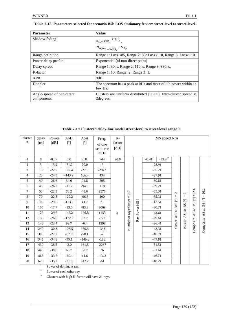
WINNER D1.1.1
Page 139 (153)
Table 7-18 Parameters selected for scenario B5b LOS stationary feeder: street-level to street-level.
Parameter Value
Shadow-fading σfree=3dB, brr ≤ ,
beyondσ=7dB, brr >
Range definition Range 1: Loss <85, Range 2: 85<Loss<110, Range 3: Loss>110.
Power-delay profile Exponential (of non-direct paths).
Delay-spread Range 1: 30ns. Range 2: 110ns. Range 3: 380ns.
K-factor Range 1: 10. Rang2: 2. Range 3: 1.
XPR 9dB.
Doppler The spectrum has a peak at 0Hz and most of it’s power within an few Hz.
Angle-spread of non-direct components.
Clusters are uniform distributed [0,360]. Intra-cluster spread is 2degrees.
Table 7-19 Clustered delay-line model street-level to street-level range 1.
cluster #
delay [ns]
Power [dB]
AoD [º]
AoA [º]
Freq.
of one scatterer
mHz
K-factor
[dB]
MS speed N/A
1 0 -0.37 0.0 0.0 744 20.0 -0.41* -33.4**
2 5 -15.9 -71.7 70.0 -5 -28.91
3 15 -22.2 167.4 -27.5 -2872 -35.21
4 20 -24.9 -143.2 106.4 434 -37.91
5 40 -26.6 34.6 94.8 295 -39.61
6 45 -26.2 -11.2 -94.0 118 -39.21
7 50 -22.3 78.2 48.6 2576 -35.31
8 70 -22.3 129.2 -96.6 400 -35.31
9 105 -29.5 -113.2 41.7 71 -42.51
10 105 -17.7 -13.5 -83.3 3069 -30.71
11 125 -29.6 145.2 176.8 1153 -42.61
12 135 -26.6 -172.0 93.7 -772 -39.61
13 140 -23.4 93.7 -6.4 1298 -36.41
14 240 -30.3 106.5 160.3 -343 -43.31
15 300 -27.7 -67.0 -50.1 -7 -40.71
16 345 -34.8 -95.1 -149.6 -186 -47.81
17 430 -38.5 -2.0 161.5 -2287 -51.51
18 440 -38.6 66.7 68.7 26 -51.61
19 465 -33.7 160.1 41.6 -1342 -46.71
20 625 -35.2 -21.8 142.2 -61
- ∞
Nu
mb
er o
f ra
ys/c
lust
er =
20
+
Ray
Po
wer
[dB
]
-48.21
clu
ster
A
S
at M
S [
º] =
2
clu
ster
A
S
at B
S [
º]
= 2
Co
mp
osi
te
AS
at
MS
[º]
=22
.4
Co
mp
osi
te
AS
at
BS
[º]
= 2
6.2
* Power of dominant ray, ** Power of each other ray
+ Clusters with high K-factor will have 21 rays.

WINNER D1.1.1
Page 140 (153)
Table 7-20 Clustered delay-line model street-level to street-level range 2.
cluster #
delay [ns]
Power [dB]
AoD [º]
AoA [º] Freq. of
one scatterer
mHz
K-factor
[dB]
MS speed N/A
1 0 -1.5 0.0 0.0 744 13.0 -1.7* -27.7**
2 5 -10.2 -71.7 70.0 -5 -23.21
3 30 -16.6 167.4 -27.5 -2872 -29.61
4 45 -19.2 -143.2 106.4 434 -32.21
5 75 -20.9 34.6 94.8 294 -33.91
6 90 -20.6 -11.2 -94.0 118 -33.61
7 105 -16.6 78.2 48.6 2576 -29.61
8 140 -16.6 129.2 -96.6 400 -29.61
9 210 -23.9 -113.2 41.7 71 -36.91
10 210 -12.0 -13.5 -83.3 3069 -25.01
11 250 -23.9 145.2 176.8 1153 -36.91
12 270 -21.0 -172.0 93.7 -772 -34.01
13 275 -17.7 93.7 -6.4 1298 -30.71
14 475 -24.6 106.5 160.3 -343 -37.61
15 595 -22.0 -67.0 -50.1 -7 -35.01
16 690 -29.2 -95.1 -149.6 -186 -42.21
17 855 -32.9 -2.0 161.5 -2288 -45.91
18 880 -32.9 66.7 68.7 26 -45.91
19 935 -28.0 160.1 41.6 -1342 -41.01
20 1245 -29.6 -21.8 142.2 -61
-∞
Nu
mb
er o
f ra
ys/c
lust
er =
20
+
Ray
Po
wer
[dB
]
-42.61
clu
ster
A
S
at M
S [
º] =
2
clu
ster
A
S
at B
S [
º]
= 2
Co
mp
osi
te
AS
at
MS
[º]
=42
.8
C
om
po
site
A
S a
t B
S [
º] =
50
.2
* Power of dominant ray, ** Power of each other ray
+ Clusters with high K-factor will have 21 rays.
Table 7-21 Clustered delay-line model street-level to street-level range 3.
cluster #
delay [ns]
Power [dB]
AoD [º]
AoA [º]
Freq. of one
scatterer mHz
K-factor
[dB]
MS speed N/A
1 0 -2.6 0.0 0.0 744 10.0 -3.0* -26.0**
2 10 -8.5 -71.7 70.0 -5 -21.51
3 90 -14.8 167.4 -27.5 -2872 -27.81
4 135 -17.5 -143.2 106.4 434 -30.51
5 230 -19.2 34.6 94.8 295 -32.21
6 275 -18.8 -11.2 -94.0 118 -31.81
7 310 -14.9 78.2 48.6 2576 -27.91
8 420 -14.9 129.2 -96.6 400 -27.91
9 630 -22.1 -113.2 41.7 71 -35.11
10 635 -10.3 -13.5 -83.3 3069 -23.31
11 745 -22.2 145.2 176.8 1153 -35.21
12 815 -19.2 -172.0 93.7 -772 -32.21
13 830 -16.0 93.7 -6.4 1298 -29.01
14 1430 -22.9 106.5 160.3 -343
-∞
Nu
mb
er o
f ra
ys/c
lust
er =
20
+
Ray
Po
wer
[dB
]
-35.91
clu
ster
A
S
at M
S [
º] =
2
clu
ster
A
S
at B
S [
º]
= 2
Co
mp
osi
te
AS
at
MS
[º]
=52
.3
C
om
po
site
A
S a
t B
S [
º] =
61
.42

WINNER D1.1.1
Page 141 (153)
15 1790 -20.3 -67.0 -50.1 -7 -33.31
16 2075 -27.4 -95.1 -149.6 -186 -40.41
17 2570 -31.1 -2.0 161.5 -2287 -44.11
18 2635 -31.2 66.7 68.7 26 -44.21
19 2800 -26.3 160.1 41.6 -1342 -39.31
20 3740 -27.8 -21.8 142.2 -61 -40.81 * Power of dominant ray, ** Power of each other ray
+ Clusters with high K-factor will have 21 rays.
7.11.3 Scenario B5c Model for B5c scenario is same with B1 LOS. Difference is that in Bfc both the environment and both link ends are stationary except two clusters, which represent moving vehicles. In these two clusters all the rays have different non-zero Doppler frequency.
Table 7-22 B5c Clustered Delay-Line model.
cluster #
delay [ns]
Power [dB]
AoD [º]
AoA [º] Freq. of one
scatterer mHz
K-factor
[dB]
MS speed N/A
1 0 0 0 0 -127 3.3 -1.67* -18.0**
2 30 -11.7 5 45 385 -24.71
3 55 -14.8 8 63 -879 -27.81
4 60 -14.8 8 -69 ++ -27.81
5 105 -13.9 7 61 +++ -26.91
6 115 -17.8 8 -69 -735 -30.81
7 250 -19.6 -9 -73 -274 -32.61
8 460 -31.4 11 92 691
-∞
Nu
mb
er o
f ra
ys/c
lust
er =
2
0+
Ray
Po
wer
[dB
]
-44.41
clu
ste
r A
S a
t M
S [º
] =
18
clu
ste
r A
S a
t B
S [º
] =
3
Co
mpo
site
AS
at
MS
[º]
=45
.0
Co
mpo
site
AS
at
BS
[º] =
4.5
* Power of dominant ray, ** Power of each other ray
+ Clusters with high K-factor will have 21 rays. ++ Frequency for 20 scatterers in Hz is 45.0, 45.5, 46.0, 46.5, … , 54.5 +++ Frequency for 20 scatterers in Hz is -55.0, -55.5, -56.0, -56.5, … , -64.5
7.11.4 Scenario B5f Model for B5f scenario is NLOS version of B5a model.
Table 7-23 Parameters selected for scenario B5f NLOS stationary feeder: rooftop to rooftop.
Parameter Value
Power-delay profile Exponential (non-direct paths).
Delay-spread 85ns
K-factor -∞ dB
XPR 10dB
Doppler A peak centreed around zero Hz with most energy within 0.1 Hz.

WINNER D1.1.1
Page 142 (153)
Table 7-24 B5f Clustered Delay-Line model. Rooftop-to-rooftop NLOS.
cluster #
delay [ns]
Power [dB]
AoD [º]
AoA [º]
Freq. of one
scatterer mHz
K-factor [dB]
MS speed N/A
1 0 -0.1 0.0 0.0 41.6 -13.11
2 10 -5.3 0.9 0.2 -21.5 -18.31
3 20 -11.5 0.3 1.5 -65.2 -24.51
4 50 -8.9 -0.3 2.0 76.2 -21.91
5 90 0.0 3.9 0.0 10.5 -13.01
6 95 -5.2 -0.8 3.6 -20.2 -18.21
7 100 -12.7 4.2 -0.7 1.3 -25.71
8 180 -3.5 -1.0 4.0 2.2 -16.51
9 205 -6.3 5.5 -2.0 -15.4 -19.31
10 260 -4.6 7.6 -4.1 48.9
-∞
Nu
mb
er o
f ra
ys /
clu
ster
= 2
0
Ray
Po
wer
[dB
]
-17.61
clu
ster
A
S
at M
S [
º] =
0.5
clu
ster
A
S
at B
S [
º]
= 0
.5
Co
mp
osi
te
AS
at
MS
[º]
= 2
.33
Co
mp
osi
te
AS
at
BS
[º]
=2
.87

WINNER D1.1.1
Page 143 (153)
8. Reference Implementation Interfaces This section describes example input and output interfaces of the WIM2 channel model function in Matlab format. Parameter sets are still incomplete and not sufficient to model all the features of the WINNER2 model.
WINNER channel model needs as an input the general information like channel scenario and MIMO setup, antenna configurations like radiation patterns and array geometries and system layout information like relative distances and orientations of the transceivers. Output of the model is a set of discrete channel impulse responses with matrix coefficients (see eq 4.13). Entries of the matrices are complex channel coefficients for each transmitter receiver antenna element pairs. Channel impulse responses are realisations of the radio channel for discrete time instants and for different radio links.
8.1.1 Example of input parameters There are four input arguments, all of which are MATLAB structures. The first three input structures (‘’wimpar’’, ‘’linkpar’’, and ‘’antpar’’) are mandatory. The following tables describe all the fields of the input structures. The most of input parameters belong to one of the following groups:
• Model (M) parameters are defined by the channel model nature itself. One example can be Number of rays per path which is fixed to 10.
• System (S) parameters are parameters defining the simulated communication system e.g., centre frequency, MS velocity etc.
• Network Layout (NL) parameters together define the simulated network. • Antenna array (AN) parameters are collection of parameters needed to define the antenna arrays
at the BS and at the MS. • Environment (E) parameters are defining the environments around BS and MS and between
them. • Implementation (I) parameters are defining the format of the output data, or improving the
implementation.
Table 8-1: General channel model parameters. Common for all links. Structure name is‘’wimpar’’, m-file name ‘’ wimparset.m’’.
Parameter name Definition Default value
Unit Parameter type
NumBsElements
The number of elements in the BS array. This parameter is ignored if antenna patterns are defined in the input struct ANTPAR. In this case the number of BS elements is extracted from the antenna definition.
2 -
AN
NumMsElements
The number of elements in the MS array. This parameter is ignored if antenna patterns are defined in the input struct ANTPAR. In this case the number of BS elements is extracted from the antenna definition.
2 -
AN
Scenario Selected WIM channel scenario (‘A1’, ‘B1’, ‘C2’ or ‘D1’)
‘A1’
-
E
range If scenario is B5b, the path-loss ranges 1, 2 and 3 are defined as in D1.1
1 E
end_time Observation end time for B5 scenario - time points are taken as: wimpar.TimeVector=linspace(0,wimpar.end_time,T);
1 second S
PropagCondition Line of sight condition (‘LOS’, ’NLOS’). Select either line of sight or non line of sight model.
‘NLOS’ - E
SampleDensity Time sampling interval of the channel. A value greater than one should be selected if Doppler analysis is to be done.
2 samples/half wavelength
S
NumTimeSamples Number of channel samples (impulse response matrices) to generate per link.
100 - S

WINNER D1.1.1
Page 144 (153)
UniformTimeSampling
If this parameter has value ‘yes’ time sampling interval of the channel for each user will be equal. Sampling interval will be calculated from the SampleDensity and the highest velocity found in the input parameter vector MsVelocity. If this parameter has value ’no’, then the time sampling interval for each link will be different, if MSs have different speeds (see userpar.MsVelocity). Setting this parameters ‘yes’ may be useful in some system-level simulations where all simulated links need to be sampled at equal time intervals, regardless of MS speeds.
‘no’ -
S
NumSubPathsPerPath Number of rays per path. The only value supported in the WIM implementation is 10 rays.
10 - M
FixedPdpUsed Use tabulated delays instead of drawing random values for each drop yes/no. If FixedPdpUsed='yes', the delays and powers of paths are taken from a table.
‘no’ - I
FixedAnglesUsed
Use tabulated angles instead of drawing random values for each drop yes/no. If FixedAnglesUsed='yes', the AoD/AoAs are taken from a table. Random pairing of AoDs and AoAs is not used.
‘no’ -
I
PolarisedArrays Defines usage of polarised arrays ‘no’ AN
CenterFrequency Carrier centre-frequency. Affects path loss and time sampling interval.
2E9 Hz System related
DelaySamplingInterval Delay sampling interval (delay resolution). 10e-8 sec I
PathLossModelUsed
Path-loss included in the channel matrices yes/no (if ‘no’, PL is calculated and returned in the second output argument, but not multiplied with the channel matrices)
‘no’ -
I
ShadowingModelUsed
Shadow fading included in the channel matrices yes/no (if ‘no’ shadow fading is still computed and returned in the second output argument, but not multiplied with the channel matrices). Note that if both path loss and shadowing are switched off the average power of the channel matrix elements will be one (with azimuthally uniform unit gain antennas).
‘no’ -
I
PathLossModel
The name of the path-loss function. Function ‘path-loss’ implements the default WIM path-loss model. If the default is used, centre-frequency is taken from the parameter CenterFrequency. One can define his/her own path-loss function. For syntax, see PATHLOSS.
‘path-loss’
-
I
PathLossOption
'RC' or 'RR_light' or 'RR_heavy', RC = Room-Corridor, RR = Room-Room nlos
'RC'
E
AnsiC_core
Use optimized computation yes/no. With ‘yes’ faster C-function is used instead of m-function. Note the C-function SCM_MEX_CORE.C must be compiled before usage. For more information, see SCM_MEX_CORE.M.
‘no’ -
I
LookUpTable
If optimized computation is used, complex exponents can be either taken from a look-up table to speed up computation or calculated explicitly. This parameter defines the table size, if 0 table is not used, if –1 default table size 214 =16384 is used. The size of the table must be a power-of-two. If AnsiC_core = ‘no’ this parameter is ignored.
0 integer
I
RandomSeed
Random seed for fully repeatable channel generation (if empty, seed is generated randomly). Note that even if RandomSeed is the fixed, two channel realizations may still not be the same between different MATLAB versions.
<empty> integer
I

WINNER D1.1.1
Page 145 (153)
Table 8-2: Link-dependent parameters. All the parameters are vectors of length K, where K is the number of links. The values are randomly generated; they are not based on any specific network geometry or user behaviour model. Structure name is ‘’linkpar’’, m-file name ‘’ linkparset.m’’.
Parameter name Definition Default value Unit Parameter type
MsBsDistance Distance between BS and MS 1965*RAND(1,K) + 35 m NL
ThetaBs θBS (see Figure 5-2) 360* RAND(1,K) deg NL
ThetaMs θMS (see Figure 5-2) 360* RAND(1,K) deg NL
MsHeight Height of the mobile station 1.5 m NL
BsHeight Height of the base station 32 m NL
MsVelocity MS velocity 10 m/s
MsDirection θv (see Figure 5-2) 360* RAND(1,K) deg NL
BsNumber
MsNumber is a positive integer defining the index number of MS for each link. This parameter is used in generation of inter-site correlated shadow fading values; shadow fading is correlated for links between a single MS and multiple BSs. There is no correlation in shadow fading between different MSs. Examples: The default value is the case where all links in a call to the SCM function correspond to different MSs. Setting MsNumber=ones(1,K) corresponds to the case where the links from a single MS to K different BSs are simulated.
[1:K] - NL
StreetWidth Street width is utilized only with path-loss model of B1.
20 m E
Dist1 This is utilized only with path-loss model of B1. Parameter is generated randomly if empty.
[empty matrix] 1xK m E
WallLoss Defines penetration losses through the ‘’light’’ and ‘’heavy’’ wall
[5 12] dB M
Table 8-3: Antenna parameters. The following parameters characterize the antennas. Currently only linear uniform arrays with dual-polarized elements are supported. The antenna patterns do not have to be identical. The complex field pattern values for the randomly generated AoDs and
AoAs are interpolated. Structure name is ‘’antpar’’, m-file name ‘’ antparset.m’’.
Parameter name Definition Default value Unit Parameter type
BsGainPattern
BS antenna field pattern values in a 4D array. The dimensions are [ELNUM POL EL AZ] = SIZE(BsGainPattern), where
ELNUM is the number of physical antenna elements in the array. The elements may be dual-polarized.
POL – polarization. The first dimension is vertical polarization, the second is horizontal. If the polarization option is not used, vertical polarization is assumed (if both are given).
EL – elevation. This value is ignored. Only the first element of this dimension is used.
AZ – complex-valued field pattern in the azimuth dimension given at azimuth angles defined in BsGainAnglesAz.
If NUMEL(BsGainPattern)=1, all elements are assumed to have uniform gain defined by the value of BsGainPattern over the full azimuth angle, and the number of BS antenna elements is defined by NumBsElements. This speeds up
1 - AN

WINNER D1.1.1
Page 146 (153)
computation since field pattern interpolation is not required.
BsGainAnglesAz
Vector containing the azimuth angles for the BS antenna field pattern values. These values are assumed to be the same for both polarizations. This value is given in degrees over the range (-180,180) degrees. If NUMEL(BsGainPattern)=1, this variable is ignored.
linspace(-180,180,90)
Deg AN
BsGainAnglesEl
Vector of elevation angles for definition of BS antenna gain values. This parameter is for future needs only; its value is ignored in this implementation (WIM does not support elevation).
- - AN
BsElementPosition
Element spacing for BS linear array in wavelengths. This parameter can be either scalar or vector. If scalar, uniform spacing is applied. If vector, values give distances between adjacent elements.
0.5 Wavelength AN
MsGainPattern
MS antenna field pattern values in a 4D array. The dimensions are [ELNUM POL EL AZ] = SIZE(MsGainPattern), where
ELNUM – the number of physical antenna elements in the array. The elements may be dual-polarized.
POL – polarization. The first dimension is vertical polarization, the second is horizontal. If the polarization option is not used, vertical polarization is assumed (if both are given).
EL – elevation. This value is ignored. Only the first element of this dimension is used.
AZ – complex-valued field pattern in the azimuth dimension given at azimuth angles defined in MsGainAnglesAz.
If NUMEL(MsGainPattern)=1, all elements are assumed to have uniform gain defined by the value of MsGainPattern over the full azimuth angle, and the number of MS antenna elements is defined by wimpar.NumMsElements. This speeds up computation since field pattern interpolation is not needed.
1 Complex AN
MsGainAnglesAz
Vector containing the azimuth angles for the MS antenna field pattern values. These values are assumed to be the same for both polarizations. This value is given in degrees over the range (-180,180) degrees. If NUMEL(BsGainPattern)=1, this variable is ignored.
linspace(-180,180,90)
Deg AN
MsGainAnglesEl
Vector of elevation angles for definition of MS antenna gain values. This parameter is for future needs only; its value is ignored in this implementation (WIM does not support elevation).
- - AN
MsElementPosition
Element spacing for MS linear array in wavelengths. This parameter can be either scalar or vector. If scalar, uniform spacing is applied. If vector, values give distances between adjacent elements.
0.5 Wavelength AN
InterpFunction
The name of the interpolating function. One can replace this with his own function. For syntax, see interp_gain.m, which is the default function. For faster computation, see interp_gain_c.m
‘interp_gain’ - I
InterpMethod
The interpolation method used by the interpolating function. Available methods depend on the function. The default function is based on MATLAB’s interp1.m function and supports e.g. ‘linear’ and ‘cubic’ (default) methods. Note that some methods, such as ‘linear’, cannot extrapolate values falling outside the field pattern definition.
‘cubic’ - I

WINNER D1.1.1
Page 147 (153)
Table 8-4: Layout parameters are defining the simulated network. Name of m-file is ‘’ layoutparset.m’’.
Parameter name Definition Default value Unit Parameter
type
BsXY matrix of BS (x,y) co-ordinates with dimensions 2xNofBs
[m] NL
NofSect vector of number of sectors in each of the BSs ones(1,NofBs) - NL
BsOmega
BsOmega is a matrix with dimensions max(NofSect)xNofBs. Each column of the matrix contains orientations of sectorised arrays with respect to some fixed North direction. If some BS have less sectors than others, the non-existing sector orientations are set to zero. E.g. setup with 2 BS, one with 1 sector and other with 3 sectors. In this case orientation matrix could be e.g. BsOmega = [11 22; 0 33; 0 44]
° NL
MsXY matrix of MS (x,y) co-ordinates with dimensions 2xNofMs
[m] NL
MsOmega vector of MS array broad side orientations ° NL
Pairing
Pairing is a matrix with dimensions NofSect x NofMs, i.e. one entry for each BS sector/MS pair. Value '1' stands for "link will be modelled" and value '0' stands for "link will not be modelled". E.g. with all ones matrix, all the MS are connected to all sectors. With e.g. first rows ones and others zeros means, that all MS are connected to only 1st sector of 1st BS.
- NL
NofMs Number of Mobile Stations 1 m NL
NofBs Number of Base Stations 1 m NL
K number of links 1 m/s NL
rmax layout range 100 [m] NL
SectPerBs default number of sectors in a BS 1 intege
r NL
BSrmin minimum distance of BSs 10 [m] NL
Parameter matrices BsGainPattern and MsGainPattern 2nd dimension is either 1 or 2. If polarization option is in use, the field pattern values have to be given for vertical and horizontal polarizations (in this order). If polarization is not used only the first dimension, i.e. vertical, is used, if both are given.
Note that the mean power of narrowband channel matrix elements (i.e. summed over delay domain) depends on the antenna gains. The default antenna has unit gain for both polarizations. Hence, the mean narrowband channel coefficient power is two for ‘polarized’ option, and one for all other options.
The fourth input argument, is optional. It can be used to specify the initial AoDs, AoAs, cisoid phases, path losses and shadowing values when WIM is called recursively, or for testing purposes. If this argument is given, the random parameter generation as defined in WIM is not needed. Only the antenna gain values will be interpolated for the supplied AoAs and AoDs.
The fields of the MATLAB struct are given in the following table. Notation: K denotes the number of links, N denotes the number of paths, M denotes the number of subpaths within a path.
Table 8-5: Initial values, fourth optional input argument.
Parameter name Definition Unit
InitDelays A K x N matrix of path delays. Sec
InitSubPathPowers A K x N x M array of powers of the subpaths. -
InitAods A K x N x M array Degrees
InitAoas A K x N x M array Degrees
InitSubPathPhases A complex-valued K x N x M array. When polarization option is used, this is a K x P x N x M array, where P=4. In this case
degrees

WINNER D1.1.1
Page 148 (153)
the second dimension includes the phases for [VV VH HV HH] polarized components.
InitPathLosses A K x 1 vector Decibel
InitShadowLosses A K x 1 vector Decibel
8.1.2 Example of output parameters There are three output arguments: CHAN, DELAYS, FULLOUTPUT. The last two are optional output parameters. Notation: K denotes the number of links, N is the number of paths, T the number of time samples, U the number of receiver elements, and S denotes the number of transmitter elements.
Table 8-6: The three output arguments.
Parameter name Definition Unit
CHAN A 5D-array with dimensions U x S x N x T x K
DELAYS A K x N vector of path delay values. Note that delays are, for compatibility with the INITVALUES, also included in FULLOUTPUT.
sec
FULLOUTPUT A MATLAB struct with the following elements:
delays A K x N matrix of path delays. This is identical to the second output argument.
sec
subPathPowers A K x N x M array of subpath powers. -
Aods A K x N x M array of subpath angles of departure degrees
Aoas A K x N x M array of subpath angles of arrival degrees
subpath_phases
A complex-valued K x N x M array giving the final phases of all subpaths. When polarization option is used, a K x P x N x M array, where P=4. In this case the second dimension includes the phases for [VV VH HV HH] polarized components.
degrees
Path_losses A K x 1 vector linear scale
shadow_fading A K x 1 vector linear scale
Delta_t A K x 1 vector defining time sampling interval for all links.
sec
Xpr A K x 2 x N array of cross-polarization coupling power ratios. The second dimension is the [V-to-H H-to-V] coupling ratios.
linear scale

WINNER D1.1.1
Page 149 (153)
9. References [3GPPSCM] 3GPP TR 25.996, “3rd Generation Partnership Project; technical specification group radio
access networks; spatial channel model for MIMO simulations (release 6)”, V6.1.0.
[AGV98] Pauli Aikio, Ralf Gruber and Pertti Vainikainen, Wideband radio channel measurements for train tunnels. VTC 1998.
[AHY06] M. Alatossava, V-M. Holappa, J. Ylitalo, “Outdoor to indoor MIMO radio channel measurements at 5.25 GHz – characterization of propagation parameters”, to be published in EUCAP, November 2006, Nice, France.
[AI00] Farrokh Abrishamkar , James Irvine, Comparison of Current Solutions for the Provision of Voice Services to Passengers on High Speed Trains. IEEE VTC-Fall, VTC 2000. 24 - 28 Sept. 2000.
[APM02] A. Algans, K. I. Pedersen, P.E. Mogensen,”Experimental analysis of the joint statistical properties of azimuth spread, delay spread and shadow fading”, IEEE J. Selected Areas in Comm., Vol. 20, pp.523-531, 2002.
[AP02] J. B. Andersen and K. I. Pedersen, “Angle-of-arrival statistics for low resolution antennas,” IEEE Trans. Antennas Propagat., vol. 50, pp. 391–395, Mar. 2002.
[Bul02] Bultitude, R.J.C., “A Comparison of Multipath-Dispersion-Related Micro-Cellular Mobile Radio Channel Characteristics at 1.9 GHz and 5.8 GHz”, in Proc. ANTEM’02, Montreal, Jul. 31 – Aug. 2, 2002, pp. 623-626.
[BBK04] M.D. Batariere, T.K. Blankenship, J.F. Kepler, T.P. Krauss,”Seasonal variations in path loss in the 3.7 GHz band”, IEEE RAWCON, pp. 399-402, 2004.
[BBK+02] M.D. Batariere, T.K. Blankenship, J.F. Kepler, T.P. Krauss, I. Lisica, S. Mukthvaram, J.W. Porter, T.A. Thomas, F.W. Vook: “Wideband MIMO mobile impulse response measurements at 3.7 GHz”, IEEE 55th VTC, pp. 26-30, 2002.
[BHS05] D. Baum, J. Hansen, J. Salo, G. Del Galdo, M. Milojvic, P. Kyösti: An Interim Channel Model for Beyond-3G Systems, IEEE VTC’05, April 2005.
[CBW95] D. J. Cichon, T. C. Beckcr, W. Wiesbeck, Determination of Time-Variant Radio Links in High-Speed Train Tunnels by Ray Optical Modeling. AP-S 1995.
[Cha03] Ashok Chandra, Propagation of 2000 MHz Radio Signal into A Multi-Storeyed building Through Outdoor-Indoor Interface. The 14” IEEE 2003 International Symposium on Personal,lndoor and Mobile Radio Communicatlon Proceedings. 2003.
[C02] M. Celidonio, “Outdoor-indoor propagation measurements in the 3.6-4.2 GHz band”, IEEE 13th PIMRC, Vol. 2, pp. 644-648, 2002.
[CKC03] A. Chandra, A. Kumar, P. Chandra, “Propagation of 2000 MHz radio signal into a multi-storeyed building through outdoor-indoor interface”, Proceedings on 14th PIMRC, Vol. 3, pp. 2983-2987, 2003.
[COST231] European Comission: European cooperation on the field of scientific and technical research (EURO-COST 231): “Digital mobile radio towards future generation systems“, Final report, http://www.lx.it.pt/cost231/, Bruxelles, 1999
[DDA00] Michael Doehler, Monica Dell’ Anna, A. H. Aghvami, Pdf - Transformation for the Outdoor-Indoor Propagation Model. VTC 2000-Spring. 2000, 15 – 18 May 2000 Pages 1646-1650 Vol. 3.
[deJKH02] Y.L.C.deJong. M.H.J.L Koelen, and M.H.J.Herben, “, “A building transmission model for improved propagation prediction in urban microcells,” IEEE Trans., Veh. Technol., vol. 53, no. 2, 2002.
[DRX98] G. Durkin, T.S Rappaport, H. Xu:”Measurements and models for radio path loss and penetration in and around homes and trees at 5.85 GHz, IEEE Trans. Comm., Vol. 46, pp.1484-1496, 1998.
WINNER D1.1.1
Page 150 (153)
[EGT+99] V. Erceg , L.J. Greenstein, S. Tjandra, S. Parkoff, A. Gupta, B. kulic, A. Julius, R. Bianci.,”An empirically based path loss model for wireless channels in suburban environments”, IEEE J. Sel. Areas Comm., Vol. 17, pp. 1205-1211, 1999.
[FDS+94] Foster, H.M.; Dehghan, S.F.; Steele, R.; Stefanov, J.J.; Strelouhov, H.K., “Microcellular measurements and their prediction”, IEE Colloquium on “Role of Site Shielding in Prediction Models for Urban Radiowave Propagation” (Digest No. 1994/231), Nov. 1994, pp. 2/1 - 2/6.
[GEA03] S. Geng et al., “ Measurements and Analysis of Wideband Indoor Radio Channels at 60 GHz,” Proc. of 3rd ESA Workshop on Millimeter Wave Technology and Applications, Espoo, Finland, May 21-23, 2003.
[GEY97] L.J. Greenstein, V. Erceg, Y.S. Yeh, M.V. Clark,”A new path-gain/delay spread model for digital cellular channels”, IEEE Trans. Veh. Tech., Vol. 46, pp. 477-485, 1997.
[GRZ07] Guo Rui Zhang, “Measurement and Characterisation of Delay, Angular and Frequency Dispersion and their Evolution at Mobile Receivers in 2.25 GHz Microcells,” M.Sc. Thesis. Report, Dept. of Systems and Computer Engineering, Carleton University, Ottawa, to be submitted, spring 2007.
[Gud91] M. Gudmundson, “Correlation model for shadow fading in mobile radio systems”, Electron. letter, vol. 27, pp. 2145-2146, Nov. 1991.
[ITU] ITU Rec. ITU-R P.1238-4.
[KeM90] J.M Keenan, A.J. Motley, “Radio coverage in buildings”, British Telecom Tech. Journal, vol.8, no.1, Jan. 1990, pp.19-24.
[KI04] K. Kitao, S. Ichitsubo,”Path loss prediction formula for microcell in 400 MHz to 8 GHz band”, Electronics Letters, Vol. 40, No. 11, 2004.
[KKM02] J. F. Kepler, T.P. Krauss, S. Mukthvaram:”Delay spread measurements on a wideband MIMO channel at 3.7 GHz”, IEEE 56th VTC, pp. 2498-2502, 2002.
[KBM+06] Sandra Knoerzer, Michael A. Baldauf, Juergen Maurer, Werner Wiesbeck, “OFDM for Multimedia Applications in High-Speed Trains: Channel Model Including Different Antenna Types.”, 2006.
[KMV+05] Sandra Knoerzer, Juergen Maurer, Sven Vogeler, Karl-Dirk Kammeyer and Werner Wiesbeck, Channel Modeling for a High-Speed Train OFDM Communication Link Supporting High Data Rates. ITST 2005.
[KP02] M. B. Knudsen, Member, IEEE, and G. F. Pedersen, Spherical Outdoor to Indoor Power Spectrum Model at the Mobile Terminal. IEEE Journal on Selected Areas in Communications, vol. 20, no. 6, August 2002.
[KRB00] A. Kuchar, J-P. Rossi, E. Bonek:”Directional macro-cell channel characterization from urban measurements”, IEEE Trans. Antennas and Propagation, Vol. 48, pp.137-145, 2000.
[KSL+02] K. Kalliola, K. Sulonen, H. Laitinen, O. Kivekäs, J. Krogerus, P. Vainikainen:”Angular power distribution and mean effective gain of mobile antenna in different propagation environments”, IEEE Trans. Veh. Techn., Vol. 51, pp.823-838, 2002.
[KZV99] J. Kivinen, X. Zhao and P. Vainikainen, “Wideband Indoor Radio Channel Measurements with Direction of Arrival Estimations in the 5 GHz Band,” Proc. of IEEE Vehicular and Technology Conference (VTC’99), pp. 2308-2312, Netherlands, 1999.
[Lan02] J. Nicholas Laneman “Cooperative Diversity in Wireless Networks: Algorithms and Architectures,” PhD thesis, sep. 2002
[Medav] http://www.channelsounder.de
[MEJ91] P.E. Mogensen, P. Eggers, C. Jensen:”Urban area radio propagation measurements for GSM/DCS 1800 macro and micro cells”, ICAP 91, pp. 500-503, 1991.
[MHA+04] J. Medbo, F. Harryson, H. Asplund, J-E. Berg, “Measurements and analysis of a MIMO macrocell outdoor-indoor scenario at 1947 MHz”, IEEE 59th VTC, Vol. 1, pp. 261-265, 2004.

WINNER D1.1.1
Page 151 (153)
[MKA02] Masui, H.; Kobayashi, T.; Akaike, M., “Microwave path-loss modeling in urban line-of-sight environments,” IEEE Journal on Selected Areas in Communications, Vol. 20, Iss. 6, Aug. 2002, pp. 1151-1155.
[MOT02] Y. Miura, Y. Oda, T. Taka, ”Outdoor-to indoor propagation modelling with the identification of path passing through wall openings”, IEEE 13th PIMRC, Vol. 1, pp. 130-134, 2002
[MRA93] L. Melin, M. Rönnlund, R. Angbratt: “Radio wave propagation – a comparison between 900 and 1800 MHz”, IEEE 43rd VTC conference, pp. 250-252, 1993.
[NAP05] H. T. Nguyen, J. B. Andersen, G. F. Pedersen, “Characterization of the indoor/outdoor to indoor MIMO radio channel at 2.140 GHz”, Department of Communication Technology, Aalborg, Denmark, 2005.
[OBL+02] J. Ojala, R. Böhme, A. Lappeteläinen and M. Uno, ”On the propagation characteristics of the 5 GHz rooftop-to-rooftop meshed network,” IST Mobile & Wireless Telecommunications Summit 2002, Jun. 2002, Thessaloniki, Greece.
[OKT+04] Ohta, G.I.; Kamada, F.; Teramura, N.; Hojo, H. 5 GHz W-LAN verification for public mobile applications - Internet newspaper on train and advanced ambulance car. Consumer Communications and Networking Conference, 2004. CCNC 2004. First IEEE. Volume , Issue , 5-8 Jan. 2004 Page(s): 569 – 574.
[OOK+68] Y. Okumura, E. Ohmori, T. Kawano, K. Fukuda:”Field strength and its variability in VHF and UHF land-mobile radio services”, Review of the Electrical Comm. Lab., Vol. 16, No 9. 1968.
[OTT+01] Y. Oda, R. Tsuchihashi, K. Tsunekawa, M. Hata,”Measured path loss and multipath propagation characteristics in UHF and microwave frequency band for urban mobile communications”, VTC 2001 Spring, Vol.1, pp. 337-341, 2001.
[Pab04] Ralf Pabst et al,”Relay based deployment concepts for wireless and mobile broadband radio,” IEEE communication magazine, Sep. 2004, pp 80-87.
[Paj03] P. Pajusco: ”Double characterisations of power angule spectrum in macrocell environment”, Electronics Letters, Vol. 39, pp. 1565-1567, 2003.
[Pap05] P. Papazian, “Basic transmission loss and delay spread measurements for frequencies between 430 and 5750 MHz”, IEEE Trans. Ant. Propagation, Vol. 53, pp. 694-701, 2005.
[PCH01] E. Perahia, D. Cox, S. Ho, “Shadow fading cross-correlation between base stations”, IEEE VTC, pp. 313-317, May 2001.
[PLB04] J.W. Porter, I. Lisica, G. Buchwald,”Wideband mobile propagation measurements at 3.7 GHz in an urban environment”, IEEE Ant. Propagat. Intern. Symposium, Vol. 4, pp. 3645-3846, 2004.
[PLN+99] M. Pettersen, P. H. Lehne, J. Noll, O. Rostbakken, E. Antonsen, R. Eckhoff, ”Characterization of the directional wideband radio channel in urban and suburban areas”, IEEE 50th VTC, pp. 1454-1459,1999.
[PMF00] K. I. Pedersen, P.E. Mogensen, B.H. Fleury, “A stochastic model of the temporal and azimuthal dispersion seen at the base statin in outdoor propagation environments”, IEEE Trans. Veh. Technol., Vol. 49, pp. 437-447, 2000.
[PT00] J. W Porter and J. A Thweatt, “Microwave Propagation Characteristics in the MMDS Frequency Band,” in Proc. IEEE ICC’00, Jun. 2000, Vol. 3, pp. 1578-1582.
[RJB89] R.J.C. Bultitude, and G.K.Bedal, “Propagation characteristics on microcellular urban mobile radio channels at 910 MHz,” IEEE J. Select. Areas Commun, vol.7, no. 1, 1989, pp. 31-39.
[RJB02] R.J.C. Bultitude., “Estimating frequency correlation functions from propagation measurements on fading radio channels: A critical review,” IEEE J. Select. Areas Commun. Vol. 20, no. 6, August, 2002, pp. 1133-1143.
[RKJ05] T. Rautiainen, K. Kalliola, J. Juntunen,”Wideband radio propagation characteristics at 5.3 GHz in suburban environments”, PIMRC Berlin, Vol. 2, pp. 868-872, 2005.

WINNER D1.1.1
Page 152 (153)
[RSS90] T. Rappaport, S. Seidel, R. Singh.,”900-MHz multipath propagation measurements fot U.S. digital cellular radiotelephone”, IEEE Trans. Veh. Technol., Vol. 39, pp.132-139, 1990.
[RJK07] T. Rautiainen, J. Juntunen, K. Kalliola, ”Propagation analysis at 5.3 GHz in typical and bad urban macrocellular environments”, submitted to VTC Dublin, 2007.
[RWH02] T. Rautiainen, G. Wölfle, R. Hoppe, ”Verifying path loss and delay spread predictions of a 3D ray tracing model in urban environment”, IEEE 56th Veh. Technol. Conf., Vol. 4, pp. 2470-2474, Sept. 2002.
[Rudd03] R.F. Rudd, “Building penetration loss for slant-paths at L-, S- and C-band.” ICAP 2003, 31.3.-1.4, 2003.
[Sau99] S. Saunders “Antenna and propagation for communication systems concept and design”, Wiley, 1999.
[SG02] S. Salous, H. Gokalp,”Dual-frequency sounder for UMTS frequency-division duplex channels”, IEE Proc. Comm., Vol. 149, pp. 117-122, 2002.
[SRJ+91] S. Seidel, T. Rappaport, S. Jain, K. Lord, R. Singh,“Path loss, scattering, and multipath delay statistics in four European cities for digital cellular and microcellular radiotelephone”, IEEE Trans. Veh. Technol., Vol. 40, pp. 721-730, 1991.
[SBA+02] Schenk, T.C.W., Bultitude, R.J.C., Augustin, L.M., van Poppel, R.H., and Brussaard, G., “Analysis of Propagation loss in Urban Microcells at 1.9 GHz and 5.8 GHz,” in Proc. URSI Commision F Open Symposium on Radiowave Propagation and Remote Sensing, Garmisch-Patenkirchen, Germany, Feb. 2002.
[SCK05] N. Skentos, Constantinou and A. G Kanatas, “Results from Rooftop to Rooftop MIMO Channel Measurements at 5.2 GHz,” COST273 TD(05)59, Bologna, Jan. 19-21.
[SCT03] A. Seville, S. Cirstea and J.F. Taylor. Effects of propagation between the indoor and outdoor environment. ICAP 2003. 31.3.-1.4. 2003.
[SG00] T. Schwengler, M. Gilbert:”Propagation models at 5.8 GHz - path loss and building penetration”, IEEE Radio and Wireless Conference 10-13 Sep. 2000, pp. 119-124.
[SJD94] E. Sousa, V. Jovanovic, C. Dainegault, “Delay spread measurements for the digital cellular channel in Toronto”, IEEE Trans. Veh. Technol., Vol. 43, pp. 837-846, 1994.
[SMI+00] H. Shimizu, H. Masui, M. Ishi, K. Sakawa, and T. Kobayashi, “LOS and NLOS Path-Loss and Delay Characteristics at 3.35 GHz in a Residential Environment,” IEEE Antennas and Propagation Society International Symposium 2000, Vol. 2, Jul. 2000, pp. 1142 - 1145.
[SMI+02] K. Sakawa, H. Masui, M. Ishii, H. Shimizu, T. Kobayashi, ”Microwave path-loss characteristics in an urban area with base station antenna on top of a tall building”, Int. Zurich Seminar on Broadband communications, pp. 31-1 -31-4, 2002.
[SMJ+99] A. M. Street, J. G. O. Moss, A. P. Jenkins, D. J. Edwards, “Outdoor-indoor wideband study for third generation communication systems”, IEE National Conference on Antennas and Propagation, pp. 128-131, 1999.
[SS01] S. Stavrou, S. R. Saunders, “A deterministic outdoor to indoor propagation modeling approach”, IEEE 54th VTC, Vol. 2, pp. 1097-1100, 2001.
[SV87] A. Saleh, and R. A. Valenzuela, A statistical model for indoor multipathpropagation, IEEE J. Select. Areas Commun., vol. SAC-5, no. 2, Feb. 1987, pp. 128–137.
[Sva02] Svantesson, T., “A double-bounce channel model for multi-polarized MIMO systems,” in Proc. IEEE VTC’02-Fall, Vol. 2, Sep. 2002, pp. 691 – 695.
[TPE02] S. Thoen, L. Van der Perre, and M. Engels, “Modeling the Channel Time-Variance for Fixed Wireless Communication”, IEEE Communication Letters, Vol. 6, No. 8, Aug. 2002.
[VKV04] L. Vuokko, J. Kivinen, P. Vainikainen., ”Results from 5.3 GHz MIMO measurement campaign”, COST273, TD(04)193, Duisburg, Germany, 20.-22.9.2004.
[WAE+04] S. Wyne, P. Almers, G. Eriksson, J. Karedal, F. Tufvesson, A. F. Molisch, “Outdoor to indoor office MIMO measurements at 5.2 GHz”, IEEE 60th VTC, pp. 101-105, 2004.

WINNER D1.1.1
Page 153 (153)
[WHL94] J.A. Wepman, J.R. Hoffman, L.H. Loew,”Characterization of macrocellular PCS propagation channels in the 1850-1990 MHz band, 3rd Annual International Conference on Universal Personal Communications, pp. 165-170, 1994.
[WHL+93] J.A. Wepman, J.R. Hoffman, L.H. Loew, W.J. Tanis, M.E. Hughes: “Impulse response measurements in the 902.928 and 1850.1990 MHz bands in macrocellular environments”, 2nd international conference on Universal Personal Communications, Vol. 2, pp. 590-594, 1993.
[WIN1D54] WINNER1 WP5: “Final Report on Link Level and System Level Channel Models” Deliverable D5.4, 18.11.2005
[WIN1D72] WINNER WP7, System assessment criteria specification, v1.0.
[WIN2IR111] WINNER2 WP1: “Propagation Scenarios“, Internal Report IR1.1.1, 22.5.2006.
[WIN2UCM] WINNER2 WP1: “Updated Channel Models”, Internal, June 2006.
[WINNERII] WINNER II Contract, Annex I – “Description of Work”, IST-4-027756, 25/10/2005.
[WAE+04] S. Wyne, P. Almers, G. Eriksson, J. Karedal, F. Tufvesson, and A. F. Molisch, Outdoor to Indoor Office MIMO Measurements at 5.2 GHz. VTC 2004-Fall. 2004 IEEE 60th Volume 1, 26-29 Sept. 2004 Pages 101-105 Vol. 1.
[WH02] J. Weitzen, T. J. Lowe, “Measurement of angular and distance correlation properties of log-normal shadowing at 1900 MHz and its application to design of PCS systems”, IEEE transactions on vehicular technology, vol. 51, No. 2, march 2002.
[WMA+05] S. Wyne, A. F. Molisch, P. Almers, G. Eriksson, J. Karedal, F. Tufvesson, “Statistical evaluation of outdoor-to-indoor office MIMO measurements at 5.2 GHz”, IEEE 61st VTC, Vol. 1, pp. 146-150, 2005.
[WOT99] G. Woodward, I. Oppermann, J. Talvitie, “Outdoor-indoor temporal & spatial wideband channel model for ISM bands”, IEEE 50th VTC, Vol. 1, pp. 136-140, 1999.
[ZEA99] X. Zhao et al, “Diffraction over typical-shaped terrain obstacles,” Journal of Electromagnetic Waves and Applications, vol. 13, pp. 1691-1707, 1999.
[Zet05] P. Zetterberg, “Auto and Multi-Site Correlation of Large Scale Parameters: Model Evolution”, Internal WINNER document, Aug. 2005.
[Xia96] H.H. Xia:” An analytical model for predicting path loss in urban and suburban environments”, Seventh IEEE Int. Symposium PIMRC, Vol 1, pp. 19.23, 1996
[XBM+94] H. Xia, H. Bertoni, L. Maciel, A. Lindsey-Steward, R. Rowe, “Microcellular propagation characteristics for personal communications in urban and suburban environments”, IEEE Trans. Veh. Technol., Vol. 43, pp- 743-752, 1994.
[YMI+04] K. Yonezawa, T. Maeyama, H. Iwai, H. Harada:” Path loss measurement in 5 GHz macro cellular systems and considerations of extending existing path loss prediction models”, IEEE WCNC, Vol. 1, pp. 279-283, 2004.
[ZKV+02] X. Zhao, J. Kivinen, P. Vainikainen, K. Skog:”Propagation characteristics for wideband outdoor mobile communications at 5.3 GHz”, IEEE Sel. Areas Comm., Vol. 20, pp. 507-514, 2002.
[ZRK+06] X. Zhao, T. Rautiainen, K. Kalliola, P. Vainikainen, ”Path-loss models for urban microcells at 5.3 GHz, IEEE Antennas and Propag. Lett., Vol. 5, pp. 152-154, 2006.