Issues in Interactive Orthogonal Graph Drawing

(Preliminary Version)

Achilleas Papakostas and Ioannis G. Tollis

Department of Computer Science The University of Texas at Dallas

Richardson, TX 75083-0688 emafl: papakost@utdallas, edu, tollis@utdallas, edu

Abstrac t . Several applications require human interaction during the design process. The user is given the ability to alter the graph as the design progresses. Interactive Graph Drawing gives the user the ability to dynamically interact with the drawing. In this paper we discuss features that are essential for an interactive drawing system. We also describe some possible interactive drawing scenaria and present results on two of them. In these results we assume that the underline drawing is always orthogonal and the maximum degree of any vertex is at most four at the end of any update operation.

1 I n t r o d u c t i o n

Graphs have been extensively used to represent various important concepts or objects. Examples of such objects include parallel computer architectures, net- works, state graphs, entity-relationship diagrams, subroutine call graphs, au- tomata, data-flow graphs, Petri nets, VLSI circuits, etc. In all of these cases, we require that the graph be represented (or drawn) in the plane so that we can understand and study its structure and properties. It is for that reason that , typically, drawing of a graph is accompanied by optimizing some cost function such as area, number of bends, number of edge crossings, uniformity in the place- ment of vertices, minimum angle, etc. For a survey of graph drawing algorithms and other related results see the annotated bibliography of Di Battista, Eades, Tamassia and Tollis [4]. An orthogonal drawing is a drawing in which vertices are represented by points of integer coordinates and edges are represented by polygonal chains consisting of horizontal and vertical line segments. In this paper we focus our attention on interactive orthogonal graph drawing.

In [17] and [19] it is shown that every biconnected planar graph of maximum degree four can be drawn in the grid with 2n + 4 bends. If the graph is not biconnected then the total number of bends rises to 2.4n + 2. In all cases, no more than four bends per edge are required. The algorithms of [19] take linear time and produce drawings, such that at most one edge may have four bends. Kant [9] shows that if the graph is triconnected of maximum degree four, then i t can be drawn on an n x n grid with at most three bends per edge. The total

420

number of bends is no more than [~nJ + 3. For planar graphs of maximum degree three it is shown in the same paper that a gridsize of (~ - 1) x ~ is sufficient and no more than ~ bends are required totally. In this case, no edge bends more than twice. Even and Granot [6] present an algorithm for obtaining an orthogonal drawing of a 4-planar graph with at most three bends per edge. If the embedding of a planar graph is fixed, then an orthogonal drawing with the minimum number of bends can be computed in O(n 2 log n) time [18]. If the planar embedding is not given, the problem is polynomially solvable for 3-planar graphs [5], and NP-hard for 4-planar graphs [8]. There is a lower bound of 2n - 2 bends for biconnected planar graphs [20].

Upper and lower bounds have been proved in the case when the orthogonal drawing of the graph is not necessarily planar. Leighton [10] presented an infinite family of planar graphs which require area g2(n log n). Independently, Leiserson [11] and Valiant [21] showed that every planar graph of degree three or four has an orthogonal drawing with area O(n log 2 n). Valiant [21] showed that the or- thogonal drawing of a general (nonplanar) graph of degree three or four requires area no more than 9n 2, and described families of graphs that require area ~(n~). Sch~iffter [16] presented an algorithm which constructs orthogonal drawings of graphs with at most two bends per edge. The area required is 2n x 2n. A better algorithm is presented in [1] and [2], which draws the graph within an n x n grid with no more than two bends per edge. This algorithm introduces at most 2n + 2 bends.

Recently, we presented an algorithm that produces an orthogonal drawing of a graph of maximum degree four that requires area no more than 0.76n 2 [14]. This algorithm introduces at most 2n + 2 bends, while the number of bends that appear on each edge is no more than two. If the maximum degree is three, then there is another algorithm which produces an orthogonal drawing which needs maximum area (~ + 1) x ~ and -~ + 3 bends [14, 15]. In this drawing, no more than one bend appears on each edge except for one edge, which may have at most two bends.

In all of the above, the drawing algorithm is given a graph as an input and it produces a drawing of this graph. If an insertion (or deletion) is performed on the graph, then we have a "new" graph. Running the drawing algorithm again will result in a new drawing, which might be vastly different from the previous one. This is a waste of time and resources from two points of view: (a) the time to run the algorithm on the new graph, and (b) the user had probably spent a significant amount of time in order to understand and analyze the previous drawing. We investigate techniques that run efficiently and introduce minimal changes to the drawing.

The first systematic approach to dynamic graph drawing appeared in [3]. There the target was to perform queries and updates on an implicit represen- tation of the drawing. The algorithms presented were for straight line, polyline and visibility representations of trees, series-parallel graphs, and planar graphs. Most updates of the data structures require O(log n) time. The algorithms main- tain the planarity of the drawing. The insertion of a single edge however, might

421

cause a planar graph to drastically change embedding, or even to become non planar. An incremental approach to orthogonal graph drawing is presented in [13], where the focus is on routing edges efficiently without disturbing existing nodes or edges.

In this paper we investigate issues in interactive graph drawing. We introduce four scenaria for interactive graph drawing, and we analyze two of them. These scenaria are based on the assumption that the underlying drawing is orthogonal and the maximum degree of any vertex is four at the end of an update operation.

We show that in one scenario (Relative-Coordinates), the general shape of the current drawing remains unchanged after an update is performed. The co- ordinates of some vertices of the current drawing may increase or decrease by at most 3 units along the x and y axes. In another scenario (No-Change), we discuss an interactive algorithm for building an orthogonal drawing of a graph from scratch, so that any update inserts a new vertex and routes new edges in the drawing without disturbing the current drawing. Our algorithm guarantees that the area of the drawing at any t ime t is no more than (n(t)+ n(t)4) 2, where n(t) is the total number of vertices at t ime t, and n(t)4 is the total number of vertices up to time t, that had degree four when they were inserted. Apart from the area, our interactive algorithm has a good performance in terms of the total number of bends which are no more than 2.66n(t)+ 2, while introducing at most 3 bends per edge.

In Sect. 2 we give an example of some features that an interactive drawing system should have. In Sects. 3 and 4 we present preliminary results on two interactive drawing scenaria. Section 5 presents conclusions and open problems.

2 I n t e r a c t i v e S c e n a r i a

First, the software which supports interactive graph drawing features should be able to create a drawing of the given graph under some layout standard (e.g., orthogonal, straight line, etc.). Secondly, the software should give the user the ability to interact with the drawing in the following ways (other interactive features are possible too):

- move a vertex around the drawing, - move a block of vertices and edges around the drawing, - insert an edge between two specified vertices, - insert a vertex along with its incident edges, - delete edges, vertices or blocks.

The drawing of the graph that we have at hand at some time moment t is called current drawing, and the graph is called current graph. The drawing resulting after the user request is satisfied is called new drawing. There are various factors which affect the decisions that an interactive drawing system takes at each moment a user request is posted and before the next drawing is displayed. Some of these factors are the following:

422

- The amount of control the user has upon the position of a newly inserted vertex.

- The amount of control the user has on how a new edge will be routed in the current drawing connecting two vertices of the current graph.

- How different the new drawing is, when compared with the current drawing.

Keeping these factors in mind, in this section we propose four different sce- naria for interactive graph drawing. They are the following:

1. The Full-Control scenario. The user has full control over the position of the new vertex in the current drawing. The control can range from specifying lower and upper bounds on the x and y coordinates that the new vertex will have, up to providing the exact desired coordinates to the system. The edges can be routed by the user or by the system.

2. The Draw-From-Scratch scenario which is based on a very simple idea: every time a user request is posted, take the new graph and draw it using one of the popular drawing techniques. Apart from the fact that this scenario gives very slow drawing systems, the new drawing might be completely different compared to the current one.

3. The [lelative-Coordina~es scenario. The general shape of the current drawing remains the same. The coordinates of some vertices and/or edges may change by a small constant because of the insertion of the new vertex (somewhere in the middle of the current drawing) and the insertion of a constant number of rows and columns.

4. The No-Change scenario. In this approach, the coordinates of the already embedded vertices, bends and edges do not change at all. In order to achieve such a property, we need to maintain some invariants after each insertion.

There is a close connection between the Full-Control scenario and global rout- ing in VLSI layout [12]. The reason is that this approach deals with (re)location of vertices and (re)routing of edges using the free space in the current drawing. Also, the technique presented in [13] computes routes for new edges inserted in the graph without disturbing any of the existing vertices and edges. The Draw- From-Scratch scenario is not interesting since every time an update is requested by the user, the drawing system ignores all the work that it did up to that point. The major disadvantage here is that the user has to "relearn" the drawing. In the rest of the paper, we discuss the other two scenaria and present preliminary results.

3 T h e R e l a t i v e - C o o r d i n a t e s S c e n a r i o

In this scenario, every time a new vertex is about to be inserted into the current drawing, the system makes a decision about the coordinates of the vertex and the routing of its incident edges. New rows and columns are inserted anywhere in the current drawing in order for this routing to be feasible. The coordinates of the new vertex (say v) as well as the locations of the new rows and/or columns will depend on the following:

423

- v's degree (at the t ime of insertion).

- How many of v's adjacent vertices Mlow the insertion of a new incident edge towards the same direction (i.e., up, down, right, or left of the vertex).

- How many of v's adjacent vertices allow a new incident edge towards opposite directions.

- Whether or not the required routing of edges can be done utilizing segments of existing rows or columns that are free (not covered by an edge).

- Our optimization criteria.

Of course, there are many different cases because there are many possible combinations. It is relatively easy to come up with various cases for each inser- tion. Instead of enumerating all of them in this section, we will give examples of some of the best and worst cases one might encounter. In the example shown in Fig. l a vertices us and ul have a free direction (edge) to the right and up respectively. In this case no new rows/columns are needed for the insertion of vertex v and no new bends are introduced. On the other hand however, in the example shown in Fig. lb all four vertices ul, us, u3 and u4 have pairwise op- posite free directions. The insertion of new vertex v requires the insertion of 3 new rows and 3 new columns in the current drawing. Additionally, eight bends are introduced. As discussed above, single edge insertions can be handled us- ing techniques from global routing [12] or the technique of [13]. The easiest way to handle deletions is to delete vertices/edges from the data structures without changing the coordinates of the rest of the drawing. Occasionaly, or on demand, the system can perform a linear-time compaction similar to the one described in [19], and refresh the screen.

i v s I U2

(a) (b)

u4

T u3

0- -

F i g . 1. Insert ion of v: (a) no new row or co lumn is required, (b) three n e w rows and three new columns are required.

424

The scenario that is described in this section maintains the general shape of the current drawing after an update (vertex/edge insertion/deletion) takes place. The coordinates of the vertices of the current drawing increase or decrease by at most 3 units along the z and y axes. This scenario works well when we build a graph from scratch, or we are presented with a drawing (which was produced somehow, perhaps by a different system) and we want our interactive system to update it. In order to refresh the drawing after each update, the coordinates of every vertex/edge affected must be recalculated.

4 T h e N o - C h a n g e S c e n a r i o

In this scenario, the drawing system never changes the positions of vertices and edges of the current drawing. It just increments the drawing by adding the new elements. This is useful in many cases where the user has already spent a lot of t ime studying a particular drawing and he/she does not want to have to deal with something completely different after each update.

There is no work known which gives satisfactory answers to the above de- scribed scenario. In this section we present a simple yet effective scheme for allowing the insertion of vertices in an orthogonal drawing so that the maximum degree of any vertex in the drawing at any time is less than or equal to four. In the description of our interactive drawing scheme, we assume that we build a graph from scratch. If a whole subgraph needs to be drawn initially, we can draw it by simulating the above scenario, inserting one vertex at a time. We assume that the graph is always connected.

An embedded vertex v has a free direction to the right (bot tom) when the grid edge that is adjacent to the right (bottom) of v is not covered by any graph edge. Let v be the next vertex to be inserted in the current graph. The number of vertices in the current graph that v is connected to, is called the local degree of v, and is denoted by local_degree(v).

Since the graph is always connected, we only consider the case where an inserted vertex has local degree one, two, three or four, except for the first vertex inserted in an empty graph. In order to prove our results, as vertices are inserted in the drawing, we maintain the following invariants:

- Every vertex of the current drawing of degree one or two has at least one free direction to the bot tom and at least one free direction to the right of the grid point where the vertex is placed.

- Every vertex of the current drawing of degree three has a free direction either to the bot tom or to the right of the grid point where the vertex is placed.

Figures 2a and 2b show the first two vertices inserted in an empty graph. Notice that after vertices vl and v2 are inserted, they both satisfy the invariants set above. Different embeddings of the first two vertices are possible but the edge that connects them always has to have one bend in the way shown in Fig. 2b. If a straight no-bend line is used to connect vl and v2, at least one of these two vertices will not satisfy the first invariant.

�9 v 1

425

l V2

(a) (b)

Fig. 2. Inserting the first two vertices in an empty graph.

Let us assume that vl is the next vertex to be inserted in the current drawing. We distinguish the following cases:

_ 1

" .... I - - - ; ' , v i

i

:V. ; 1

(a) (b)

Fig.3. The insertion of local degree one vertex v, requires one one column and one r O W .

1. vi has local degree one. There are two cases which are shown in Figs. 3a and 3b. At most one new column and one new row are required, and at most one bend is introduced. Notice that this bend is introduced along an edge which is incident to vi and whose other end is open. In Fig. 3a the vertex will have one free direction to the bot tom and two to the right. The second free direction to the right (which is responsible for introducing an extra row and bend to the drawing) will be inserted in the drawing later and only if vi

turns out to be a full blown degree four vertex. We take a similar approach for the second downward free direction of vi of Fig. 3b.

2. vi has local degree two. There are four cases. We have shown two cases in Figs. 4a and 4b (the other two are symmetric and are treated in a similar fashion). At most one new row and one new column is required, and at most two bends are introduced along edges which are incident to vi and connect vi with the current drawing.

426

I I ~ I I

I U 1 " i . t ' u2�9 I f I I I L I _ 1 L

V

V. (a) (b) 1

Fig. 4. (a) The insertion of local degree two vertex vi requires one column; (b) the insertion of vi now requires one column and one row.

3. vi .has local degree three. There are nine cases. All cases, however, can be treated by considering just two cases, as shown in Fig. 5: (a) all the vertices have a free edge in the same direction (right or down), and (b) two vertices have a free edge in the same direction (right or down) and the other vertex has a free edge in the opposite direction (down or right). The rest of the cases are symmetr ic and are treated in a similar fashion. At most one new row and one new column are required, and at most three bends are introduced along edges which are incident to vi and connect vl with the current drawing.

4. vi has locM degree four. There are sixteen cases. All cases, however, can be treated by considering just three cases, as shown in Fig. 6: (a) all the vertices have a free edge in the same direction (right or down), (b) three vertices have a free edge in the same direction (right or down) and one vertex has a free edge in the other direction (down or right), and (c) two vertices have a free edge in the same direction (right or down) and the other two vertices have a free edge in the other direction (down or right). The symmetr ic cases are treated in a similar fashion. At most two new rows and two new columns are required, and at most six bends are introduced along edges which are incident to vi and connect vl with the current drawing.

As we described above, the easiest way to handle deletions is to delete ver- tices/edges from the data structures without changing the coordinates of the rest of the drawing. Occasionaly, or on demand, the system can perform a linear-time compaction similar to the one described in [19], and refresh the screen.

L e m m a 1. The total number of bends introduced by the algorithm for the "No- Change scenario" up to time t is at most 2.66n(t) + 2, where n(l) is the number of vertices at time t.

T h e o r e m 2. There exists a simple interactive orthogonal graph drawing scheme for the "No-Change scenario" with the following properties:

1. evc~j insertion operation lakes constant time,

427

U3=

ua= U 1

1 _I

I

u3�9 , I

I u 2 : ,

a T ' I

(a) (b)

"V. 1

Fig. 5. (a) The insertion of local degree three vertex v, requires one column; (b) the insertion of v~ now requires one row and one column.

e u 4 I

;Tvi U 1 ~ i

I . . . . . . . . I

U3~- u4= :

I

: i _ _,,,

Tvi (a) (b) (c)

Fig.6. (a) The insertion of local degree four vertex v, requires two columns; (b) the insertion of v, requires two columns and one row; (c) the insertion of vi requires two columns and two rows.

2. every edge has at most three bends, 3. the total number of bends at any time t is at most 2.66n(t) + 2, where n(t)

is the number of vertices of the drawing at time t, and ~. the area of the drawing at any time t is no more than (n(t) + n(t)4) 2, where

n(t)4 is the number of vertices of local degree .~ which have been inserted up to time t.

The interactive scheme we just described is simple and efficient. The area and bend bounds are higher than the best known [1, 2, 14, 15], but we have to consider that this is a scheme that gives the user a lot of flexibility in inserting any node at any time. Moreover, any insertion takes place without disturbing the current drawing, since the insertion is built around it. Besides, n(t)4 is the number of vertices of local degree four which have been inserted up to time t, and not the total number of vertices of degree four in the graph. The area will be much smaller if the user chooses an insertion strategy which keeps n(t)4 low.

428

6

5 3

(a)

i i~~i~i : :? i : : : i i i i

i i i l . ! : : : - : : : : e - - : - - . : : - - - : ' . . i ::i:::: ....... l-I----7---- i , ....... T--T i~i . . . . . . . . . I . . . . . . . t T . . . . . . . . . . . . . t ,~.

T

Co)

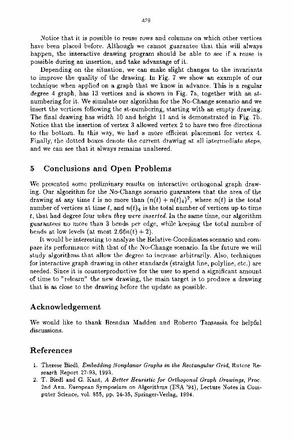
Fig. 7. (a) A regular graph of degree 4 with 13 vertices, (b) drawing the graph with the algorithm of the No-Change scenario

429

Notice that it is possible to reuse rows and columns on which other vertices have been placed before. Although we cannot guarantee that this will always happen, the interactive drawing program should be able to see if a reuse is possible during an insertion, and take advantage of it.

Depending on the situation, we can make slight changes to the invariants to improve the quality of the drawing. In Fig. 7 we show an example of our technique when applied on a graph that we know in advance. This is a regular degree 4 graph, has 13 vertices and is shown in Fig. 7a, together with an st- numbering for it. We simulate our algorithm for the No-Change scenario and we insert the vertices following the st-numbering, starting with an empty drawing. The final drawing has width 10 and height 11 and is demonstrated in Fig. 7b. Notice that the insertion of vertex 3 allowed vertex 2 to have two free directions to the bottom. In this way, we had a more efficient placement for vertex 4. Finally, the dotted boxes denote the current drawing at all intermediate steps, and we can see that it always remains unaltered.

5 Conclusions and Open Problems

We presented some preliminary results on interactive orthogonal graph draw- ing. Our algorithm for the No-Change scenario guarantees that the area of the drawing at any time t is no more than (n(t) + n(t)4) 2, where n(t) is the total number of vertices at t ime t, and n(t)4 is the total number of vertices up to time t, that had degree four when they were inserted. In the same time, our algorithm guarantees no more than 3 bends per edge, while keeping the total number of bends at low levels (at most 2.66n(t) + 2).

It would be interesting to analyze the Relative-Coordinates scenario and com- pare its performance with that of the No-Change scenario. In the future we will study algorithms that allow the degree to increase arbitrarily. Also, techniques for interactive graph drawing in other standards (straight line, polyline, etc.) are needed. Since it is counterproductive for the user to spend a significant amount of t ime to "relearn" the new drawing, the main target is to produce a drawing that is as close to the drawing before the update as possible.

Acknowledgement

We would like to thank Brendan Madden and Roberto Tamassia for helpful discussions.

References

1. Therese Biedl, Embedding Nonplanar Graphs in the Rectangular Grid, Rutcor Re- search Report 27-93, 1993.

2. T. Biedl and G. Kant, A Better Heuristic for Orthogonal Graph Drawings, Proc. 2nd Ann. European Symposium on Algorithms (ESA '94), Lecture Notes in Com- puter Science, vol. 855, pp. 24-35, Springer-Verlag, 1994.

430

3. R. Cohen, G. DiBattista, R. Tamassia, and I. G. Tollis, Dynamic Graph Drawing, to appear in SIAM Journal on Computing.

4. G. DiBattista, P. Eades, R. Tamassia and I. Tollis, Algorithms for Draw- in9 Graphs: An Annotated Bibliography, Computational Geometry: Theory and Applications, vol. 4, no 5, 1994, pp. 235-282. Also available via anony- mous ftp from ftp.cs.brown.edu, gdbiblio.tex.Z and gdbiblio.ps.Z in /pub/papers/compgeo.

5. G. DiBattista, G. Liotta and F. Vargiu, Spirality of orthogonal representations and optimal drawings of series-parallel graphs and 8-planar graphs, Proc. Workshop on Algorithms and Data Structures, Lecture Notes in Computer Science 709, Springer- Verlag, 1993, pp. 151-162.

6. S. Even and G. Granot, Rectilinear Planar Drawings with Few Bends in Each Edge, Tech. Report 797, Comp. Science Dept., Technion, Israel Inst. of Tech., 1994.

7. S. Even and R.E. Tarjan, Computing an st-numbering, Theor. Comp. Sci. 2 (1976), pp. 339-344.

8. A. Garg and R. Tamassia, On the Computational Complexity of Upward and Rec- tilinear Planarity Testing, Proc. DIMACS Workshop GD '94, Lecture Notes in Comp. Sci. 894, Springer-Verlag, 1994, pp. 286-297.

9. Goos Kant, Drawing planar graphs using the lmc-ordering, Proc. 33th Ann. IEEE Syrup. on Found. of Comp. Science, 1992, pp. 101-110.

10. F. T. Leighton, New lower bound techniques ]or VLSI, Proc. 22nd Ann. IEEE Syrup. on Found. of Comp. Science, 1981, pp. 1-12.

11. Charles E. Leiserson, Area-Efficient Graph Layouts (/or VLSI}, Proc. 21st Ann. IEEE Syrup. on Found. of Comp. Science, 1980, pp. 270-281.

12. Thomas Lengauer, Combinatorial Algorithms ]or Integrated Circuit Layout, John Wiley and Sons, 1990.

13. K. Miriyala, S. W. I-Iornick and R. Tamassia, An Incremental Approach to Aes- thetic Graph Layout, Proc. Int. Workshop on Computer-Aided Software Engineer- ing (Case '93), 1993.

14. A. Papakostas and I. G. Toms, Algorithms for Area-Efficient Orthogonal Drawings , journal version, in preparation.

15. A. Papakostas and I. G. Tollis, Improved Algorithms and Bounds ]or Orthooonal Drawings, Proc. DIMACS Workshop GD '94, Lecture Notes in Comp. Sci. 894, Springer-Verlag, 1994, pp. 40-51.

16. Markus Sch~ffter, Drawing Graphs on Rectangular Grids, Discr. Appl. Math. (to appear).

17. J. Storer, On minimal node-cost planar embeddings, Networks 14 (1984), pp. 181- 212.

18. R. Tamassia, On embeddin 9 a graph in the grid with the minimum number of bends, SIAM J. Comput. 16 (1987), pp. 421-444.

19. R. Tamassia and I. Toms, Planar Grid Embeddings in Linear Time, IEEE Trans. on Circuits and Systems CAS-36 (1989), pp. 1230-1234.

20. R. Tamazsia, I. Tollis and J. Vitter, Lower Bounds for Planar Orthogonal Drawings of Graphs, Information Processing Letters 39 (1991), pp. 35-40.

21. L. Valiant, Universality Considerations in VLSI Circuits, IEEE Trans. on Comp., vol. C-30, no 2, (1981), pp. 135-140.