issues in flow and transport in heterogeneous porous media
TRANSCRIPT
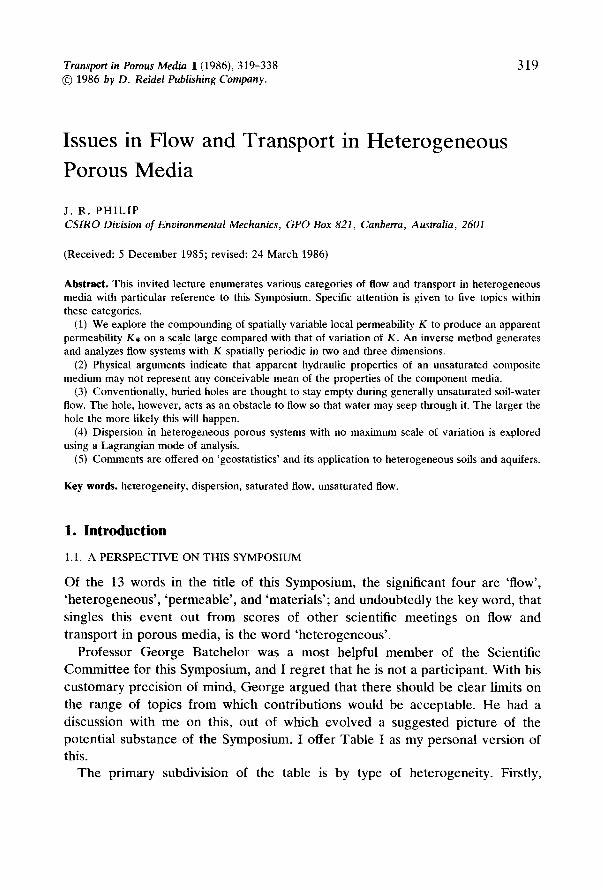
Transport in Porous Media 1 (1986), 319-338 3 19 �9 1986 by D. Reidel Publishing Company.
Issues in Flow and Transport in Heterogeneous Porous Media
J. R. PHILIP CSIRO Division of Environmental Mechanics, GPO Box 821, Canberra, Australia, 2601
(Received: 5 December 1985; revised: 24 March 1986)
Abstract. This invited lecture enumerates various categories of flow and transport in heterogeneous media with particular reference to this Symposium. Specific attention is given to five topics within these categories.
(1) We explore the compounding of spatially variable local permeability K to produce an apparent permeability K , on a scale large compared with that of variation of K. An inverse method generates and analyzes flow systems with K spatially periodic in two and three dimensions.
(2) Physical arguments indicate that apparent hydraulic properties of an unsaturated composite medium may not represent any conceivable mean of the properties of the component media.
(3) Conventionally, buried holes are thought to stay empty during generally unsaturated soil-water flow. The hole, however, acts as an obstacle to flow so that water may seep through it. The larger the hole the more likely this will happen.
(4) Dispersion in heterogeneous porous systems with no maximum scale of variation is explored using a Lagrangian mode of analysis.
(5) Comments are offered on 'geostatistics' and its application to heterogeneous soils and aquifers.
Key words, heterogeneity, dispersion, saturated flow, unsaturated flow.
1. Introduction
1.1. A PERSPECTIVE ON THIS SYMPOSIUM
Of the 13 words in the t i t le of this Sympos ium, the s igni f icant four a re ' f low' ,
' h e t e r o g e n e o u s ' , ' p e r m e a b l e ' , and ' m a t e r i a l s ' ; and u n d o u b t e d l y the key word , tha t
s ingles this e v e n t ou t f rom scores of o t h e r scientif ic m e e t i n g s on flow and
t r a n s p o r t in p o r o u s med ia , is the w o r d ' h e t e r o g e n e o u s ' .
P ro fes so r G e o r g e B a t c h e l o r was a mos t he lpfu l m e m b e r of the Scient if ic
C o m m i t t e e for this Sympos ium, and I r e g r e t tha t he is no t a pa r t i c ipan t . W i t h his
c u s t o m a r y p r ec i s i on of mind , G e o r g e a r g u e d tha t t he re should be c l ea r l imits on
the r ange of top ics f rom which con t r i bu t i ons w o u l d be a c c e p t a b l e . H e had a
d i scuss ion wi th m e on this, ou t of wh ich e v o l v e d a s u g g e s t e d p i c tu re of the
po ten t i a l subs t ance of the Sympos ium. I offer T a b l e I as m y pe r sona l ve r s ion of
this.
T h e p r i m a r y subd iv i s ion of the tab le is by type of h e t e r o g e n e i t y . Firs t ly ,
320
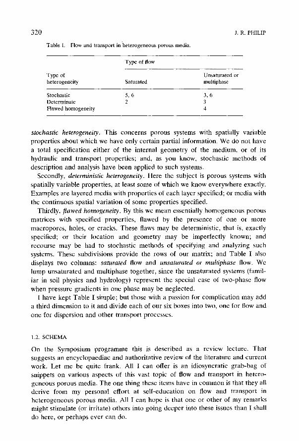
Table I. Flow and transport inheterogeneous porous media.
J. R. PHILIP
Type of flow
Type of Unsaturated or heterogeneity Saturated multiphase
Stochastic 5, 6 3, 6 Determinate 2 3 Flawed homogeneity 4
stochastic heterogeneity. This concerns porous systems with spatially variable properties about which we have only certain partial information. We do not have a total specification either of the internal geometry of the medium, or of its hydraulic and transport properties; and, as you know, stochastic methods of description and analysis have been applied to such systems.
Secondly, deterministic heterogeneity. Here the subject is porous systems with spatially variable properties, at least some of which we know everywhere exactly. Examples are layered media with properties of each layer specified; or media with
the continuous spatial variation of some properties specified. Thirdly, flawed homogeneity. By this we mean essentially homogeneous porous
matrices with specified properties, flawed by the presence of one or more macropores, holes, or cracks. These flaws may be deterministic, that is, exactly specified; or their location and geometry may be imperfectly known; and
recourse may be had to stochastic methods of specifying and analyzing such systems. These subdivisions provide the rows of our matrix; and Table I also displays two columns: saturated flow and unsaturated or multiphase flow. We lump unsaturated and multiphase together, since the unsaturated systems (famil- iar in soil physics and hydrology) represent the special case of two-phase flow
when pressure gradients in one phase may be neglected. I have kept Table I simple; but those with a passion for complication may add
a third dimension to it and divide each of our six boxes into two, one for flow and
one for dispersion and other transport processes.
1.2. SCHEMA
On the Symposium programme this is described as a review lecture. That suggests an encyclopaediac and authoritative review of the literature and current work. Let me be quite frank. All I can offer is an idiosyncratic grab-bag of snippets on various aspects of this vast topic of flow and transport in hetero- geneous porous media. The one thing these items have in common is that they all derive from my personal effort at self-education on flow and transport in heterogeneous porous media. All I can hope is that one or other of my remarks might stimulate (or irritate) others into going deeper into these issues than I shall
do here, or perhaps ever can do.
FLOW AND TRANSPORT IN HETEROGENEOUS MEDIA 321
The following Sections 2-6 are my five snippets. The numerals on Table I indicate where they fit into the range of topics of this Symposium.
2. Compounding Heterogeneities in Saturated Flow
One interesting issue concerns the matter of how a three-dimensional jigsaw puzzle of bits and pieces of different permeability add up to produce an apparent mean permeability of the whole medium. Obviously this question is meaningful only when the scale of variation of the local permeability, K, is small compared with the overall scale of the macroscopic flow system to which we seek to attribute this overall constant, this apparent permeability, K . .
People have investigated series arrangements, parallel arrangements, and series-parallel arrangements; and this approach may be useful in establishing inequalities. More sophisticated studies of composite materials have dealt with (the equivalent of) the apparent permeability of a matrix with K = K1 containing inclusions of a material with K = K2 # Kj. In addition, many investigators have found empirically, or assumed, or offered theoretical arguments, that K is log-normally distributed. This has implications for the compounding of the K's to yield K . .
In order that these distributions should vary on a scale small compared with the overall scale of the macroscopic flow system, we require that the pattern of K be periodic in the appropriate number of dimensions. Then, with the scale of the pattern small relative to that of the overall flow system, it suffices for us to analyze a flow which is one-dimensional in the large.
One can generate any spatially periodic K and solve the equation
V. (KV~) = 0 (1)
within the basic unit cell, subject to suitable periodic boundary conditions. Almost inevitably it would be necessary to carry out the calculations numerically by computer. My interest has been to see what might be done in closed form, and this led to the following inverse method.
2.1. INVERSE METHOD OF GENERATING PERIODIC K: TWO DIMENSIONS
Rectangular space coordinates x, y are such that x is in the macroscopic flow direction. The components of flow velocity in the x, y directions are u, v; and the stream function �9 and potential qb are defined through
u = O~/Oy = - K O~/ax; v = -Oq~lOx = - K O~lOy. (2)
We now specify the stream function as
X p = y + a s i n x s i n y , 0 < a < ~ l , (3)
which describes flow in a medium with K of period 2zr in both x and y. The differential equation for any equipotential ~ = constant is then
322 J.R. PHILIP
d y _ 0 0 / 0 x _ 1 + a sin x cos y (4)
dx 0@/0y a cos x sin y
The solution of (4) is
- a cos y = C cos x + sin x, (5)
with C(O) the constant of integration.
Now each increment 27r in x corresponds to a constant decrement in O, so x
can enter (5) only in linear combination with O. The only possible form of C(O) is therefore
C = tan(bO + c) (6)
with b, c constants, which makes (5)
- a cos(bOp+ c) cos y = sin(bOp+ c + x). (7)
Without loss of essential generality, we take
C = tan Op, (8)
since putting c nonzero merely adds an arbitrary constant to Op; and putting b # 1 merely multiplies Op by b - t and multiplies K by b. Our solution is thus
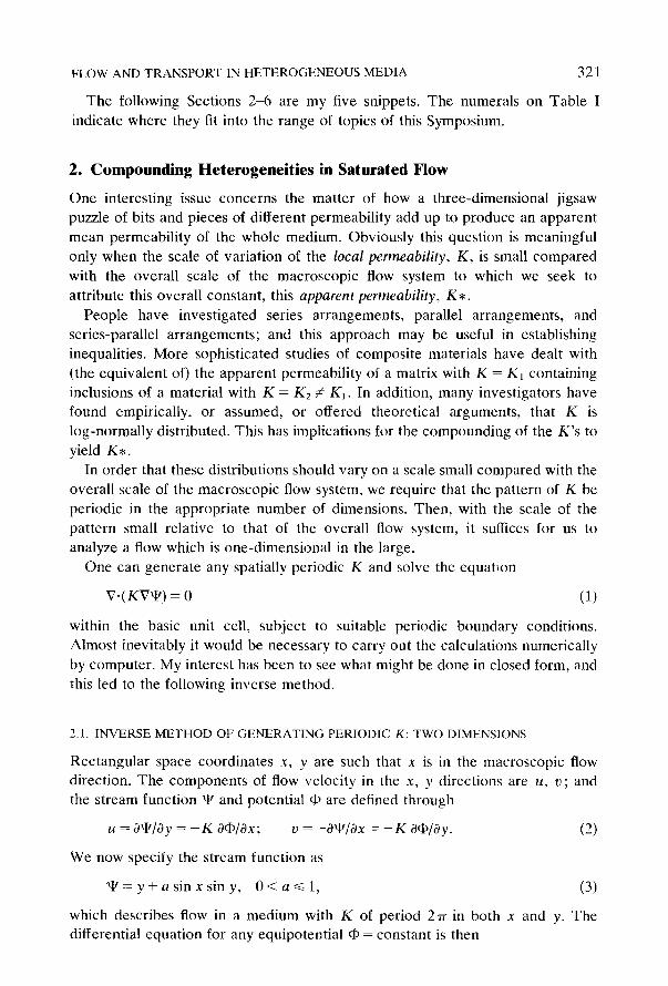
Fig. 1. The periodic distribution of permeabili ty K described by (12) with a = 1. The arrow indicates the macroscopic flow (x) direction. Numerals on the curves denote values of K. Light shading indicates regions 2.5 ~< K <~ 4, heavy shading regions with 0 ~< K <~ 0.5. The figure depicts a region of dimensions 3~rx 2~-.
F L O W A N D T R A N S P O R T IN H E T E R O G E N E O U S M E D I A 323
x = - c b - s in - l ( a cos ~ cos y), [sin-~l <~ �89 (9)
Now, f rom the second of (2),
OqqOx a cos x sin y K O~lOy O~P/ay ' (10)
and, f rom (7) with b = 1, c =-0,
Oqb a cos x sin y - - = , ( 1 1 ) 0y 1 + 2 a sin x cos y + a 2 cos z y
so that
K = 1 + 2 a sin x cos y + a 2 cos 2 y. (12)
Equa t ion (12) gives the pat tern of var ia t ion of K, with values f rom ( 1 - a) 2 to
(1 + a) 2. No te that, by put t ing b = 1, we have made K , = 1. Figure 1 shows the
pa t te rn of K for a = 1.
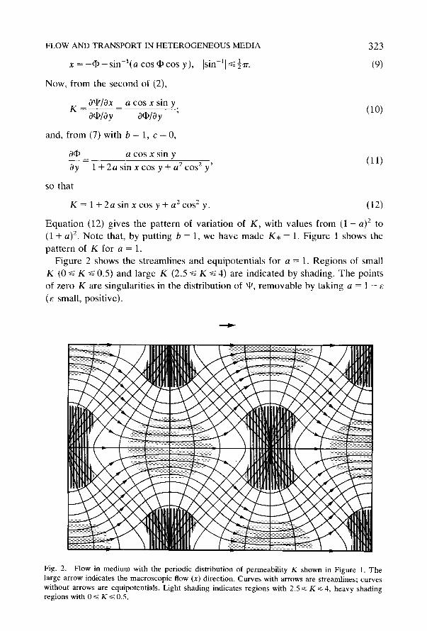
Figure 2 shows the streamlines and equipotent ia ls for a = 1. Regions of small
K (0 <~ K ~< 0.5) and large K (2.5 ~< K ~< 4) are indicated by shading. The points
of zero K are singularities in the distr ibution of qs, r emovab le by taking a = 1 - e
(e small, positive).
Fig. 2. Flow in medium with the periodic distribution of permeabili ty K shown in Figure 1. The large arrow indicates the macroscopic flow (x) direction. Curves with arrows are streamlines; curves without arrows are equipotentials. Light shading indicates regions with 2.5 ~< K ~< 4, heavy shading regions with 0 ~< K ~< 0.5.
324 J.R. PHILIP
2.2. THE CONJUGATE SOLUTION
A second flow with periodic permeabi l i ty follows readily. The t ransformat ion
~ - d O , d~---~--q L
changes (2) to
O~/Oy = u = - K10d~/Ox,
x ~ y, y ~ x, K - + K 1 1 (13)
- O ~ / O x = v = - K I O~/Oy; (14)
and it follows that a second per iodic system has s t ream funct ion
y = q ~ - s in - l ( a cos q~ cos x) (15)
and potential
qb = - x - a sin x sin y. (16)
Equat ions (15) and (16) are (3) and (9) t ransformed th rough (13). It follows that,
for this second solution,
K1 = [1 + 2a cos x sin y + a 2 cos 2 x] -1. (17)
Note that here also K , = 1, with the range of K~ f rom (1 + a) -2 to ( 1 - a ) -2.
Here also we have al ternat ing regions of low and high permeabi l i ty on a square
lattice. T he pat tern of distr ibution of K1 and of q~ and qb are simply genera ted by
ro ta t ion and relabelling of those for K given by (12) (i.e., of Figures 1 and 2 in
the case a = 1).
2.3. THE DISTRIBUTION OF K AND Ki
We calculate the distribution density of K , f ( K ) in closed form. The a lgebra is
compl ica ted , but the final result is the surprisingly simple
(1 - a) 2 ~< K ~< (1 + a) 2 , f ( K ) = r r - 2 a - l K - 1 / 4 K ( k ) . (18)
Here
[ ~2 K(k) = (1 - k 2 sin 0) 1/2 dO dO
is the comple te elliptic integral of the first kind and
k 2 _ ( K 1/2 + 1)2[a 2 - (KI/2 _ 1) 2]
4aZ KX/2
For a = 1, (18) reduces to
0 <~ K <~ 4 , f ( K ) = " r r - 2 K - 1 / a K ( k ) (19)
FLOW AND T R A N S P O R T IN H E T E R O G E N E O U S M E D I A 325
C
LL
0.8
0,6 m
0.4 --
0 .2 --
0
- 5
i
-4 -3
i I 1 1 [
J I [ i
-2 -I 0 I
fn K , - I n K I
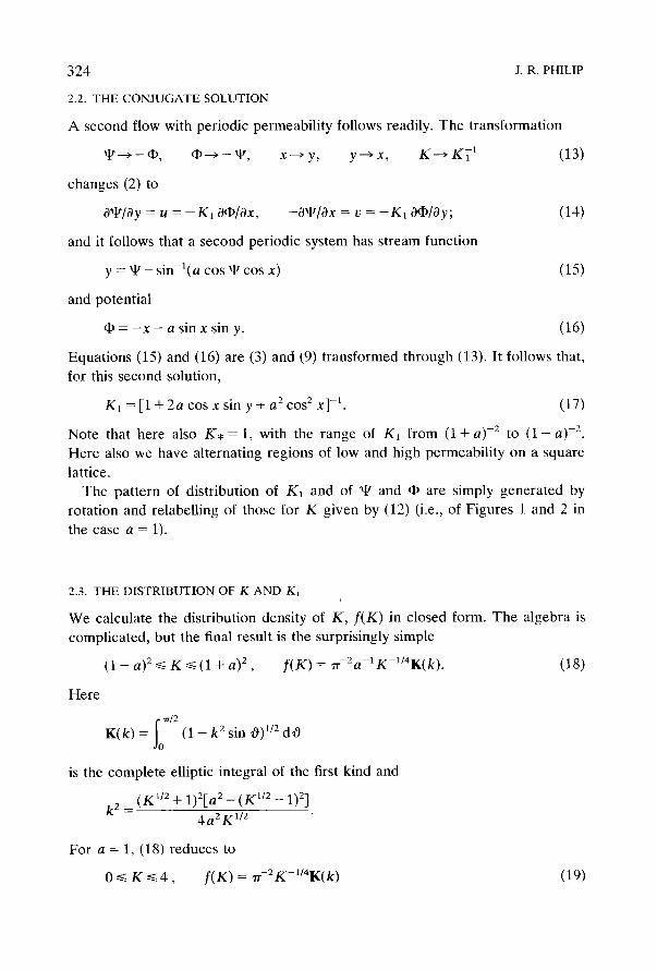
Fig. 3. Distribution of In K and - In K~, K described by (12) and K~ by (17), in each case for a = 1.
with
k 2 = �88 - K l / 2 ) ( 1 + K t / 2 ) 2.
The distribution of KI is simply the distribution of K -1. Figure 3 shows on the one graph, for the case a = 1, the distribution of In K and - l n K1.
2.4. V A R I A N C E S , C O V A R I A N C E S , AND C O R R E L A T I O N S
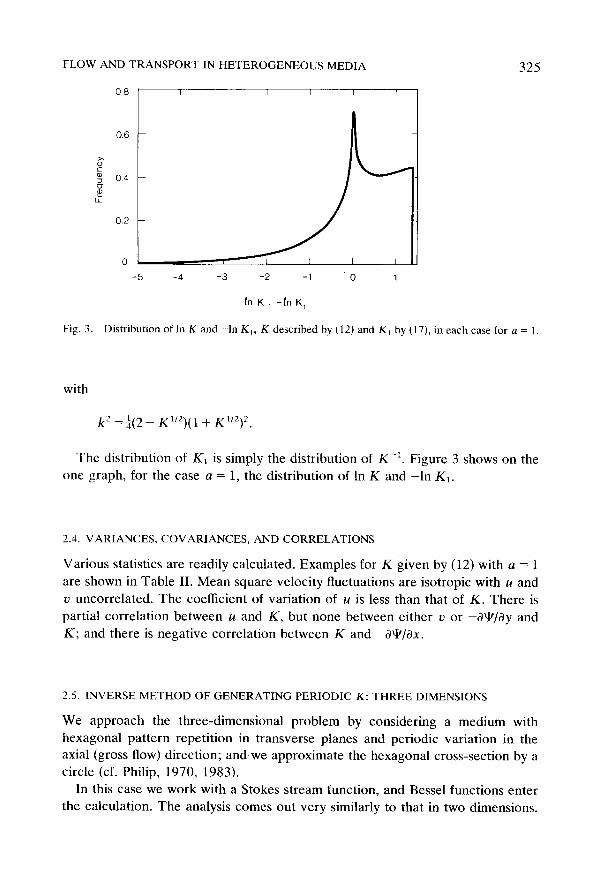
Various statistics are readily calculated. Examples for K given by (12) with a = 1
are shown in Table II. Mean square velocity fluctuations are isotropic with u and v uncorrelated. The coefficient of variation of u is less than that of K. There is
partial correlat ion between u and K, but none between either v or -09q3y and K; and there is negat ive correlation between K and -O~/Ox.
2.5. INVERSE M E T H O D OF G E N E R A T I N G PERIODIC K: T H R E E DIMENSIONS
We approach the three-dimensional problem by considering a medium with hexagonal pat tern repetit ion in transverse planes and periodic variation in the axial (gross flow) direction; and we approximate the hexagonal cross-section by a circle (cf. Philip, 1970, 1983).
In this case we work with a Stokes s t ream function, and Bessel functions enter the calculation. The analysis comes out very similarly to that in two dimensions.
326
Table II. Statistics of flow with periodic K given by (12) with a = 1
J. R. PHILIP
Quantity Value Remarks
g ~ cf K , = 1 var(K)
3 tr(K) 24--2 ~ 1.0607
1 o'(K)/_K ~__ ~ 0.7071 coeff, of variation
t 0
var(u) �88 var(v) cov(u, v) 0 ~(u)/a
,/2 r(K, u) - - ~ 0.4714
3 r(K, c) 0
O~/Ox 1 OcblO y 0 cov(K, O~/Ox)
coy(K, a~lOy) 0
mean square velocity fluctuation is isotropic velocity components uncorrelated less than coeff, of var. of K
correlation partial
no correlation
negative correlation between positive quantities K and -a~/ax no correlation
q = ar i thmet icmean; var(q) = ( q - ~ )2 ; r = [var( q ) ] t / z ; coy(p, q) = Pq - / ) q ; r(p, q) = coy(p, q)[var(p) var(q)] -1/2 .
3. Compounding Heterogeneities in Unsaturated Flows
3.1. THE QUESTION OF 'ADDITIVITY '
At a workshop in Canberra on soil physics and field heterogeneity I showed that, for good physical reasons, unsaturated flow properties in a medium layered
transverse to the flow cannot compound in any way that is remotely like additive. My talk was published subsequently (Philip, 1980), but, to judge from the recent literature, it has gone over like a lead balloon.
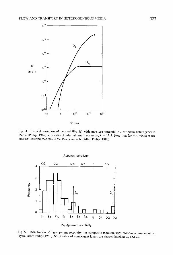
To put the matter in the simplest terms, there is continuity of potential across an interface between a fine-textured unsaturated subvolume of the medium and a coarse-textured one, but there is no t continuity of permeability (hydraulic conductivity). It is only very near saturation that the permeability of the coarse medium exceeds that of the fine: over most of the potential range the coarse material is the less permeable. See Figure 4.
The consequence is that, in unsteady unsaturated flow systems spanning any significant range of moisture potential, every change of texture in the flow
327
K
(ms -1)
10-5
10-6
10-7
10- 8
10"9
c- r
O" (9
I J_
10-10
- 1 0
I I
-1 -10 -1 -10 -2 -10 -3
(m)
Fig. 4. Typical variation of permeability K, with moisture potential ~, for scale-heterogeneous media (Philip, 1967) with ratio of internal length scales A2/A~ = 13.5. Note that for ~ < - 0 . 4 8 m the coarser-textured medium is the less permeable. After Philip (1980).
Apparent sorptivity
i - 3 1 - 4 i-5 1-6 i.7 i 8 7 . 9 0 0 - 1 0 2 0 - 3
0.2 0-3 0.5 0-7 1 1.5 4 7 ~ T 1 3 T
FLOW AND TRANSPORT IN H E T E R O G E N E O U S MEDIA
1 0 -4 i i I
log Apparent sorptivity
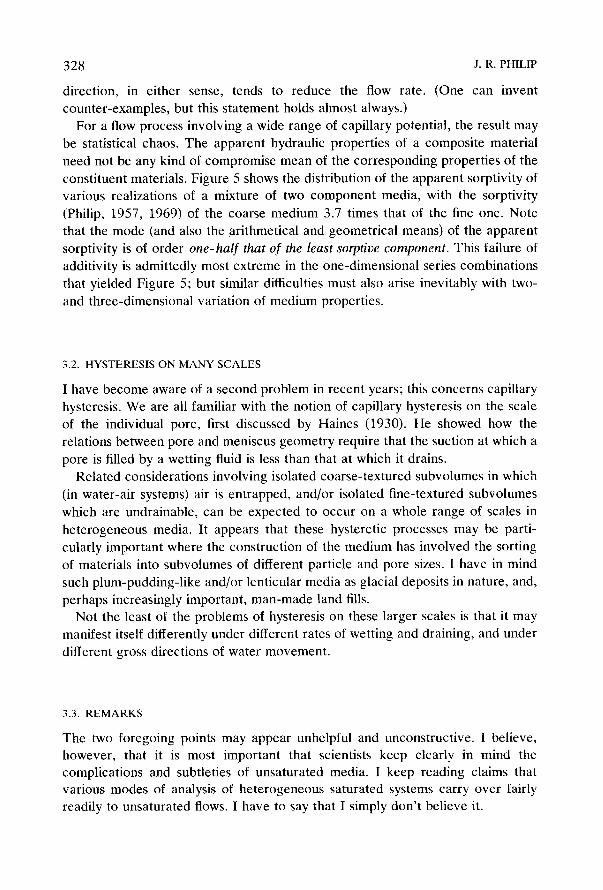
Fig. 5. Distribution of log apparent sorptivity, for composite medium, with random arrangement of layers, after Philip (1980). Sorptivities of component layers are shown, labelled A~ and A 2.
328 J . R . PHILIP
direction, in either sense, tends to reduce the flow rate. (One can invent counter-examples, but this statement holds almost always.)
For a flow process involving a wide range of capillary potential, the result may be statistical chaos. The apparent hydraulic properties of a composite material need not be any kind of compromise mean of the corresponding properties of the constituent materials. Figure 5 shows the distribution of the apparent sorptivity of various realizations of a mixture of two component media, with the sorptivity
(Philip, 1957, 1969) of the coarse medium 3.7 times that of the fine one. Note that the mode (and also the arithmetical and geometrical means) of the apparent
sorptivity is of order one-half that of the least sorptive component. This failure of additivity is admittedly most extreme in the one-dimensional series combinations that yielded Figure 5; but similar difficulties must also arise inevitably with two-
and three-dimensional variation of medium properties.
3.2. HYSTERESIS ON MANY SCALES
I have become aware of a second problem in recent years; this concerns capillary hysteresis. We are all familiar with the notion of capillary hysteresis on the scale of the individual pore, first discussed by Haines (1930). He showed how the relations between pore and meniscus geometry require that the suction at which a pore is filled by a wetting fluid is less than that at which it drains.
Related considerations involving isolated coarse-textured subvolumes in which (in water-air systems) air is entrapped, and/or isolated fine-textured subvolumes
which are undrainable, can be expected to occur on a whole range of scales in heterogeneous media. It appears that these hysteretic processes may be parti- cularly important where the construction of the medium has involved the sorting of materials into subvolumes of different particle and pore sizes, l have in mind such plum-pudding-like and/or lenticular media as glacial deposits in nature, and,
perhaps increasingly important, man-made land fills. Not the least of the problems of hysteresis on these larger scales is that it may
manifest itself differently under different rates of wetting and draining, and under
different gross directions of water movement.
3.3. REMARKS
The two foregoing points may appear unhelpful and unconstructive. I believe, however, that it is most important that scientists keep clearly in mind the complications and subtleties of unsaturated media. I keep reading claims that various modes of analysis of heterogeneous saturated systems carry over fairly readily to unsaturated flows. I have to say that I simply don' t believe it.
FLOW AND TRANSPORT IN HETEROGENEOUS MEDIA
,iiiii' .ili! i!ii i ii !i!ii . ii i i)iiiiiiiii ii)ii!ii iii!i i iiii!-iii!;i;
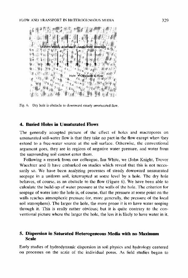
Fig. 6. Dry hole is obstacle to downward steady unsaturated flow.
329
4. Buried Holes in Unsaturated Flows
The generally accepted picture of the effect of holes and macropores on unsaturated soil-water flow is that they take no part in the flow except when they extend to a free-water source at the soil surface. Otherwise, the conventional
argument goes, they are in regions of negative water pressure, and water from the surrounding soil cannot enter them.
Following a remark from our colleague, Ian White, we (John Knight, T revor
Waechter and I) have embarked on studies which reveal that this is not neces- sarily so. We have been analyzing processes of steady downward unsaturated seepage in a uniform soil, interrupted at some level by a hole. The dry hole behaves, of course, as an obstacle to the flow (Figure 6). We have been able to calculate the build-up of water pressure at the walls of the hole. The criterion for seepage of water into the hole is, of course, that the pressure at some point on the walls reaches atmospheric pressure (or, more generally, the pressure of the local soil atmosphere). The larger the hole, the more prone it is to have water seeping through it. This is really rather obvious; but it is quite contrary to the con- ventional picture where the larger the hole, the less it is likely to have water in it.
5. Dispersion in Saturated Heterogeneous Media with no Maximum Scale
Early studies of hydrodynamic dispersion in soil physics and hydrology centered on processes on the scale of the individual pores. As field studies began to
330 J .R. PHILIP
accumulate, however, it became clear that dispersion, and the apparent diffusivi-
ties, were much greater than could be explained on the basis of individual pore processes.
The explanation, of course, resides in the heterogeneities of the soil or aquifier on scales much larger than the pore scale; and a great deal of work has been done on this; and we shall hear a lot about it at this Symposium.
The matter, however, can be taken further. There is a significant body of evidence suggesting that the larger the flow region considered, the greater the apparent diffusivities; and the mean square dispersion appears to increase as some power of time, or travel distance, significantly greater than one, perhaps a power as large as 1.5. This is against the background that models involving a maximum scale must, at least asymptotically, lead to the mean square dispersion increasing in direct proportion to time (or distance).
People fond of models involving (either explicitly or implicitly) a finite maxi- mum scale have been known to argue as follows: Well, maybe there isn't a maximum scale; but, if we postulate one, we are being conservative in the sense that we shall underestimate the ease with which pollutants can be dissipated into the environment; and therefore we shall help keep the polluters and the environmental authorities on their toes.
But this cuts both ways. What if there is a source of pollution, say 20 km from some area, perhaps a city water supply, or a densely populated zone, which you quite definitely want to keep absolutely free of pollution. Do you really want to underestimate the potential spread of the pollution plume?
This fourth snippet brings together two rather disparate elements, one classical and the other from a currently fashionable field. Firstly, I use a Lagrangian approach to dispersion rather than the more common Eulerian one. Lagrangian statistics are more relevant to dispersion processes: their intimate connexion with dispersion was established for once and for all in G. I. Taylor 's famous 1921 paper (Taylor, 1921). His classical result connecting mean square dispersion and the Lagrangian velocity autocorrelation function is used in what follows. The fashionable ingredient here comes from the world of fractals (Mandelbrot, 1975, 1983). I am supposing that our medium is fractal in character, in the sense that there is no preferred length-scale of the variation of its properties. The im- plication is that sample volumes of any size are assumed to look 'equally heterogeneous' .
5.1. THE LAGRANGIAN LOSS OF CORRELATION
We are concerned with a steady flow, one-dimensional in the large. We begin by supposing that the medium is so structured that it exhibits a finite number of separate and distinct Lagrangian time scales, Ti, each corresponding in some sense to a length scale of variation of medium properties.
F L O W A N D T R A N S P O R T IN H E T E R O G E N E O U S M E D I A 331
We concern ourselves with flow velocity component u with spatial fluctuations u' so that
u ' = u - a. (20)
Here, and in what follows, overbars signify arithmetic spatial means. We now treat u' as the superposition of separate contributions u'i, each associated with a particular Ti. Thus
u ' = ~ u',. (21) i
We now assert that each contribution is statistically independent of all other contributions so that
u',u~ =-- O, i ~- j. (22)
Now for each u~ we have a Lagrangian autocorrelation function
u',( to) U',( to + t) R,( t ) = , t>lO. (23) (u',) 2
Here t denotes time. We also have that the Lagrangian autocorrelation function for the total flow,
u'(to)U'(to + t) R ( t ) = , t >i O. (24)
( u ' ) 2
Putting (21), (22), (23) in (24), we find
R ( t ) = •i (u ' , )2Rdt) _ ~, f~R,(t), (25) (u') 2
where the quantity
- (u'~)2 with Z ~ =- 1 (26)
represents the fraction of total velocity variance contributed by the ith com- ponent.
If we assume exponentional loss of correlation for each component , so that
R d t ) = e-", ' , with ni = T71, (27)
(25) becomes
R ( t ) = ~. f, e-",'. ( 2 8 ) i
The n~ are then m o d e numbers of exponential loss of correlation.
332 J.R. PHILIP
We now take these ideas to the limit where the discrete ni become a con-
tinuous range f rom 0 to 2, and the discrete f~ become the distribution density function f(n). Then (28) becomes
R(t) = Io f(n) e - " ' dn, (29)
so that f(n) is the inverse Laplace transform of R(t). We see that f(n) is a spectrum of mode numbers of exponential loss of correlation. Note that we have
a Laplace spectrum, not the customary Fourier one.
5.2. THE AUTOCORRELATION FUNCTION
We may proceed f rom this point in various ways. Here we recognize that there is
a minimum Lagrangian scale T , , extrinsic to the medium, but arising f rom our
methods of defining, measuring, and sampling local attributes of the system such
as permeability, flow velocity components , potential, and solute concentration.
T , is thus related to a length characteristic of our sampling and observat ion
procedures.
We then find that the condition of no preferred length or time scale intrinsic to
the medium itself leads to a power law spectrum, truncated at the maximum mode number n , = T . 1. Accordingly
= , O ~ n < ~ n , , O < a < l , n ,
= 0 , n > n , .
Note that (30) implies
I ) f(n) dn =- 1,
as we require. Combining (29) and (30) we then obtain
(1 - a) ["* R ( t ) - -nT* - ~ ~o n -'~ e-"' d n
= (1 - a)~'"-1~/(1 - a , r), with ~- = n,t .
Here the incomplete gamma function
T(a, x) = e -y ya-1 dy.
In the special case a = �89 (32) reduces to
R(r) = �89 erf(~-l/e).
(30)
(31)
(32)
(33)
FLOW AND TRANSPORT IN HETEROGENEOUS MEDIA 333
io-'
10 -2 - -
10 -2
I I I I I ] /
/
~ = 0.4 _
i 1 I ",~ i i
10 -1 1 10 10 2 10 3 10 4
T
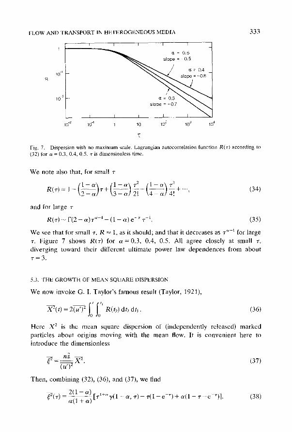
Fig. 7. Dispersion with no maximum scale. Lagrangian autocorrelation function R(r) according to (32) for a = 0.3, 0.4, 0.5. r is dimensionless time.
W e note also that , for small r
_(l-~r +(1-c~'~r 2 (1-c~)r 3 R ( r ) = l \ 2 - c z ] \ 3 - c z / 2 . T - ~ ~ + ' ' ' (34)
and for la rge r
R(r) ~ F(2 - c~)r ~-~ - (1 - a ) e - T r-~. (35)
W e see tha t for smal l r , R ~ 1, as it should ; and that it dec r ea se s as r ~--~ for la rge
r . F igu re 7 shows R(r) for ~ = 0 . 3 , 0.4, 0.5. Al l ag ree c lose ly at small r,
d i v e r g i n g t o w a r d thei r d i f fe ren t u l t ima te p o w e r law d e p e n d e n c e s f rom abou t
"/" ~ 3 .
5.3. THE GROWTH OF MEAN SQUARE DISPERSION
W e now invoke G. I. T a y l o r ' s f amous resul t (Tay lor , 1921),
Io'Io' X2(t) = 2(u ' ) 2 R(t2) dt2 d h .
Here X 2 is the mean square
pa r t i c l es abou t or ig ins m o v i n g
i n t roduce the d imens ion les s
9
~ __n~ X~" (u ') 2
T h e n , c o m b i n i n g (32), (36), and (37), we l ind
- 2 ( 1 - ~) [ r l+~ r ) r ( 1 - e - ' ) + ~ ( 1 - r - e - D ] . ~:2(T) a (1 + c~) y(1 - c~, -
(36)
d i spe r s ion of ( i n d e p e n d e n t l y re leased) m a r k e d
with the m e a n flow. It is c o n v e n i e n t here to
(37)
(38)
334 J.R. PHILIP
The special case of a = �89 gives
- - 3 . _ e _ , ) ] . ~2('T) = 4['D'l/2T3/2 erf(,r|/2) - -r(~--e- ) + �89 (39)
We find, for small r,
1 - a 1 - a ] ~-2('r) = 'r 2 1 3 ( 2 - a~' r4 1 2 ( 3 - a ) ' r 2 + " " ' (40)
and, for large ~-,
~(z) 2F(2- a) ~_,,+1 2(1- a) 2 (1- a) �9 - - 1-4- - - (41)
a ( l + a ) a a + l
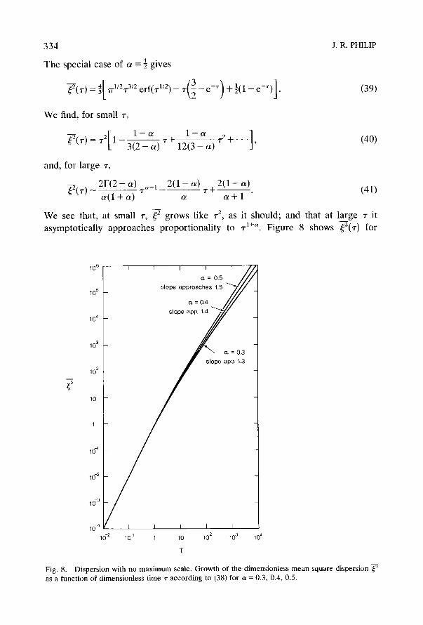
W e see that, at smal l ~-, ~2 g r o w s l ike z 2, as it should; and that at large z it
asymptotically approaches proportionality to ~.1+,. Figure 8 shows ~2(z) for
~2
10 6
10 5
10 4
10 3
10 2
10
1
lo-2
10 -3
10 -4
i i I I I
~ : 0.5
slope approaches6=0.4 z~1"5~/
slope app. 1.4
\ 6 = 0 . 3 slope app. 1.3
10 -2 10 -1 1 10 102 103 104
T
Fig. 8. D ispers ion w i th no m a x i m u m scale. G r o w t h o f the d imensionless mean square d ispers ion ~2
as a f unc t i on o f d imensionless t ime ~" accord ing to (38) fo r a = 0.3, 0.4, 0.5.
FLOW AND TRANSPORT IN HETEROGENEOUS MEDIA 335
= 0.3, 0.4, 0.5. All agree closely at small -r and d ive rge toward their u l t imate
p o w e r law d e p e n d e n c e s at abou t r = 50.
5.4. THE APPARENT DIFFUSIVITY
T h e dispers ion we are cons ider ing m a y be desc r ibed by an appa ren t diffusion coeff icient D, which is an increas ing func t ion of t (or r) . W e have, in fact , that
i t 1 d
D(t ) = ( b / ' ) 2 R ( h ) dtl = ~ ~ (X2(t)). (42) )
It then follows f r o m (38) that
( u ' ) 2 1 - c~ D ( r ) - [ r~y(1 - or, r ) - 1 + e - ' ] . (43)
/,/g, ot
T h e case ot = ~ gives
(u')2 rrX/~rl/2 erf r 1:~ D ( r ) = [ - ( - ) - l + e - T ] . (44) n ,
For small t, (43) r educes to
D(t ) ~ 2(u ' )e t (45)
as it should; and for la rge -r, we find
D ( r ) - (u')2 [F(2 - oz)'r ~ + ~ - 1], (46) o~n~
yielding D(t ) asympto t ica l ly increas ing as t%
5.5. OTHER FORMS OF R(r)
Of course any R ( r ) with similar p o w e r law b e h a v i o u r at large "r will yield the
des i red a sympto t i c power law g rowth of m e a n square dispersion. No te that we
m a y total ly d iscard the fo rego ing a r g u m e n t and s imply adopt , directly, a
L a g r a n g i a n au toco r r e l a t i on func t ion with the requ i red p roper ty . A n example is
R ( r ) = (1 + r ) "-1, 0 < a < 1. (47)
This gives
r - 2 [(1 + r) l+~ - (1 + a ) r - 1], (48) ,~(1 + a)
which also has the power law at t r ibutes we are seeking. Note that, if we insist on an in te rp re ta t ion of (47) in t e rms of a spec t rum of
336
modes of exponential loss of correlation, we now find
J. R. PHILIP
1 n e-~/"* (49) f ( n ) - n , r (1 - a)
In this case we again find a basically power-law spectrum, but, in place of the n = n , cutoff, it is the exponential factor e -n/"* which effectively removes the contributions from large n (very small ~-).
I repeat that the required behaviour depends only on the asymptotic power-law form of R(~-), not on the model of correlation loss used in Section 5.1. That model at least has the virtue that it is consistent with the concept of a fractal medium with no special length scales, with the spectral cut-off determined by the methods of definition, sampling, and measurement.
6. Geostatistics, Especially l~iging
My final snippet concerns what is fashionably labelled 'geostatistics'. You will be aware that an arcane practice called 'kriging' has a large place in this geostatis- tics. Many of you will know Wilford Gardner, the distinguished U.S. soil physicist. I heard him give a seminar recently in which he had occasion to mention kriging. In his inimitable way he said: "Well, I don't know a lot about kriging; but it sure sounds like one of those pastimes that used to be both illegal and immoral, but isn't any more."
I have become aware of the emergence in the literature of soil physics and hydrology in recent years of strange rites (with their own strange terminology) practiced on field data subject to the vagaries of spatial variability. Until recently, I was quite prepared to mind my own business and watch broadmindedly without comment - on the principle of 'whatever turns you o n . . . ' .
I have, however, been jolted out of my indifference by the work of my younger brother, Graeme, and his colleague David Watson, of the Department of Geology and Geophysics, Sydney University. I ask forgiveness for indulging briefly in what, I suppose, is scientific nepotism. Whereas I am the mildest of persons, my little brother tends to be rather forthright. He and Watson have recently published five papers on what they perceive as the inflated claims for the intellectual worth, the theoretical validity, and the practical efficiency of kriging and related procedures (G. M. Philip and Watson, 1984a, 1984b, 1986a, 1986b, 1986c).
It is of some interest that the Theory of Regionalized Variables (Matheron, 1965) has become the subject of a study within the history and philosophy of science. It has been seen in that context as an example of an aberrant theory created by an in-group and successfully promulgated to an untutored clientele (Shurtz, 1984). Inter al ia, Shurtz writes:
FLOW AND TRANSPORT IN HETEROGENEOUS MEDIA 337
We now ask how a theory with so many manifest aberrations has attracted so many devotees willing to make it a life's work. The answer appears to lie in the opacity of the mainly superfluous mathematical screen behind which the theory is sequestered. Those inside see out, and those outside see in - if they see at all - only as through a glass darkly. As has been said in another connection, this very vagueness makes the theory eminently suited to become the scriptures of a new religion.
These are fighting words; and, I speedily add, they are not mine. Here I merely plead for scepticism rather than uncritical acceptance and evangelism.
Within the soil physics/hydrology context I perceive difficulties, not only with kriging, but with other attempts at stochastic analysis.
I am obliged to say that, in my view, awkward questions about stationarity, and various efforts to save the day by subtracting out trends, miss the deeper, more fundamental, issue. As I see it, the really deep-seated difficulty is that the practical user of these activities, when there is one, is concerned with how to understand what is going on in a particular one-off landscape. This means that, at least as far as the hydraulics is concerned*, there is absolutely no possibility of ergodicity. There is no notionally unbounded ensemble of realizations of the process; there is not even a finite ensemble. There is simply one reality.
References
Haines, W. B., 1930, Studies in the physical properties of soil. V. The hysteresis effect in capillary properties, and the modes of moisture distribution associated therewith, J. Agr. Sci. 20, 97-116.
Mandelbrot, B. B., 1975, Les objects fractals: Forme, hasard et dimension, Flammarion, Editeur, Paris. Mandelbrot, B. B., 1983, The Fractal Geometry of Nature, W. H. Freeman, San Francisco. Matheron, G., 1965, Les variables regionalis~es et leur estimaaon, Masson, Paris. Philip, G. M. and Watson, D. F., 1984a, Drilling patterns and ore reserve measurements, Proc.
Australas. Inst. Min. Metall. No. 289, 205-211. Philip, G. M. and Watson, D. F., 1984b, Some limitations in the geostatistical evaluation of ore
deposits, Int. J. Mining Eng. 3, 155-159. Philip, G. M. and Watson, D. F., 1986a, Matheronian statist ics-quo vadis?, Math. Geol. 18, 93-117. Philip, G. M. and Watson, D. F., 1986b, Comment on 'Comparing splines and kriging', Comput.
Geosci. 12, 243-245. Philip, G. M. and Watson, D. F., 1986c, Automatic interpolation methods for mapping piezometric
surfaces, Automatika, In press. Philip, J. R., 1957, The theory of infiltration: 4. Sorptivity and algebraic infiltration equations, Soil
Sci. 84, 257-264. Philip, J. R., 1967, Sorption and infiltration in heterogeneous media, Aust. J. Soil Res. 5, 1-10. Philip, J. R., 1969, Theory of infiltration, Adv. Hydrosci. 5, 215-296. Philip, J. R., 1970, Diffuse double-layer interactions in one-, two-, and three-dimensional particle
swarms, J. Chem. Phys. 52, 1387-1396. Philip, J. R., 1980, Field heterogeneity: some basic issues, Water Resour. Res. 16, 443-448.
* I concede that dispersion processes offer some limited possibilities of ergodicity, thanks to molecular diffusion and to bifurcation of streamlines at every stagnation point in the highly multiply-connected flow channel.
338 J .R. PHILIP
Philip, J. R., 1983, 'Infiltration in One, Two, and Three Dimensions', in Advances in Infiltration, Proc. Nat. Conf. Adv. Infiltration, Chicago, Am. Soc. Agric. Eng., St. Joseph, Michigan, pp. 1-13.
Shurtz, R. F., 1984, 'A Stochastic Aberration-the Theory of Regionalized Variables', paper presented to Section L (History and Philosophy of Science), Pacific Division, AAAS, Annual Meeting, Mimeo., 12 pp.
Taylor, G. I., 1921, Diffusion by continuous movements, Proc. Lond. Math. Soc. 20, 196-211.