investment under uncertainty and the value of real …€¦ · investment under uncertainty and the...
TRANSCRIPT
Investment under Uncertaintyand the Value of Real and Financial Flexibility∗
Patrick Bolton† Neng Wang‡ Jinqiang Yang§
May 27, 2014
Abstract
We develop a model of investment under uncertainty for a financially constrained
firm. Facing external financing costs, the firm prefers to fund its investment through
internal funds, so that the firm’s optimal investment policy and value now depend
on both its earnings fundamentals and liquidity holdings. We show that financial con-
straints significantly alter the standard real options results, with the financial flexibility
conferred by internal funds acting as a complement, and at times as a substitute, to
the real flexibility given by the optimal timing of investment. We show that: 1) the
investment hurdle (whose deviation from the first-best Modigliani-Miller benchmark
measures investment distortions) is highly nonlinear and non-monotonic in the firm’s
internal funds, as the firm may prefer accumulating internal funds rather than access-
ing external capital markets to finance investment when internal funds are sufficiently
high; 2) with multiple rounds of growth options, a value-maximizing financially con-
strained firm may choose to over-invest via accelerated investment timing in earlier
stages in order to mitigate under-investment problems in later stages.
∗First Draft (December, 2012) was circulated under the title “Investment, Liquidity, and Financingunder Uncertainty.” We thank Ilona Babenka, Martin Cherkes, Sudipto Dasgupta, Peter DeMarzo, DirkHackbarth, Mark Gertler, Simon Gilchrist, Vicky Henderson and seminar participants at American FinanceAssociation (AFA) 2014 meetings in Philadelphia, Boston University, Columbia University, HKUST 2013Finance Symposium, Rutgers University, University of Cambridge, University of Minnesota Carlson School,and Zhejiang University for helpful comments.†Columbia University, NBER and CEPR. Email: [email protected]. Tel. 212-854-9245.‡Columbia Business School and NBER. Email: [email protected]. Tel. 212-854-3869.§The School of Finance, Shanghai University of Finance and Economics (SUFE). Email:
1 Introduction
In their influential textbook Dixit and Pindyck (1994) condense the essence of investment
decisions to three key attributes: i) the degree of irreversibility ; ii) the risk over future
revenue; and, iii) the flexibility in the timing of the decision. In this paper we add a
fourth attribute: the funding cost of the investment. Much of the real-options-based theory
of investment under uncertainty following McDonald and Siegel (1986) assumes that firms
operate in frictionless capital markets. This is for good reason, as the firm’s investment
decision can then be formulated as a simple real option problem involving the optimal exercise
and valuation of an American option. The option pricing tools developed by Black and
Scholes (1973) and Merton (1973) can then be deployed to analyze the real options problem.
A major limitation of this approach, however, is that firms in practice do not operate
in frictionless capital markets. They face significant external financing costs and as a result
may often rely on internal funds and internally generated (current and future) cash flows to
finance their investments. The recent financial crisis is an important reminder of how severe
external financing costs can be in extreme situations and how much they can affect corporate
investment and the macroeconomy. The extensive surveys of chief financial officers (CFOs)
by Graham and Harvey (2001, 2002) have also revealed the great importance CFOs attach to
maintaining financial flexibility. Thus, while determining the value of real flexibility obtained
from the optimal timing of irreversible investments one cannot abstract from the requirement
of financial flexibility to be able to fully take advantage of real options. Accordingly, the
important theoretical question we address in this paper is how corporate investment decisions
and the valuation of investments under uncertainty are affected by external financing costs
and the firm’s efforts to relax these costs by dynamically managing its liquidity holdings. In
effect, we are integrating two classical strands of literature, one started by Miller and Orr
(1966) on corporate cash balances and the other started by McDonald and Siegel (1986) on
real options.
Although the classical tools of option pricing theory can no longer be directly applied
(and although the analysis of the investment problem and its financing involves solving a
considerably more involved two-dimensional partial differential equation), the results we ob-
tain are intuitive and striking. First, both the growth options in the start-up phase and the
abandonment options in the mature phase of the firm’s life-cycle are worth less when the
firm faces external financing constraints. Second, the firm is more likely to abandon an asset
1
(captured by a higher abandonment hurdle) when the firm faces external financing costs:
The firm facing external financing costs is capitalizing expected future external financing
costs and setting these against the present value of the asset. However, should the finan-
cially constrained firm decide to continue operating the asset when it runs out of cash by
raising external funds, the firm will tend to raise more external funds the higher are external
financing costs, as the firm seeks to limit the risk of having to return to capital markets again
in the future. Third, with multiple rounds of growth options, a financially constrained firm
may surprisingly lower the hurdle for early investments (a form of over-investment) in order
to gain access to higher operating cash-flows and thus mitigate under-investment problems
in later stages.
Fourth, the hurdle for investment in the start-up phase is a non-monotonic function of
the firm’s stock of liquid assets: When the firm’s internal funds are sufficient to entirely cover
the costs of the investment then the firm’s hurdle for investment is lower the higher the firm’s
internal funds. In contrast, when the firm’s internal funds cannot cover the entire cost of the
investment then the hurdle may be sharply increasing with the firm’s internal funds. The
reason is that when the firm is approaching the point where it may be able to entirely fund
its investment with retained earnings it has a strong incentive to delay investment until it has
sufficient funds to be able to entirely avoid tapping costly external funds. This is in our view
the most striking effect of the presence of external financing costs. An important implication
of this result is that investment is not necessarily more likely when the firm has more cash.
Investment could well be delayed further, as the firm’s priority becomes avoiding reliance on
external funds. In sum, for firms facing external financing costs the value of an investment
opportunity is not just tied to timing optionality but also to flexibility, which depends on
both the financial ability to seize an investment opportunity and on timing optionality.
Our analysis contributes to the literature on financial frictions and corporate investment
in the vein of Fazzari, Hubbard, and Petersen (1988), Froot, Scharfstein, and Stein (1993),
and Kaplan and Zingales (1997). These models are purely static and thus not are set up to
study the value of financial and real flexibility, which arises from the optionality of investment
and financing decisions.
While all static financial-constraint-based models unambiguously predict that firms under-
invest due to costly external financing, we show that a financially constrained firm may over-
invest as doing so allows the firm to accumulate more internal funds sooner which in turn
mitigate the the firm’s under-investment distortions in the future. This dynamic mechanism
2
is important as it highlights that ignoring the firm’s ability to adjust its financing margin
(accumulating internal funds versus issuing external equity) significantly changes the impact
of financial constraints on investment decisions. Put differently, in a dynamic setting, a firm
has multiple margins to adjust its decisions. Hence an empirical hypothesis (e.g., that a
firm underinvests due to financial constraints based on static models) can be mis-leading.
Also our dynamic model predicts that the firm’s flexibility with regard to its real investment
timing decision (summarized by the optimal investment threshold policy) is non-monotonic
in the firm’s internal funds, again due to the firm’s intertemporal financial flexibility (by ac-
cumulating internal funds rather than having to access external equity). Third, the amount
of equity financing is also non-monotonic in its internal funds in our model, also due to the
firm’s real and financial flexibilities. The firm’s option to access external financing is highest
when its real option value is moderate. The intuition is as follows. For a firm whose invest-
ment option is sufficiently out of the money, financial flexibility has little value to the firm.
On the other hand, a firm whose investment option is deep in the money, the option value
of accumulating internal funds is of little value. Therefore, the multiple options of financing
(internal versus external as well as the flexible timing decision of external financing) are most
valuable for a firm whose real option value is in the medium range. The positive synergies
between the real and financial option values are the greatest in the medium range.
Related literature. Following Brennan and Schwartz (1985) and McDonald and Siegel
(1986) the basic formulation of the investment under uncertainty problem has been extended
in many different directions. Majd and Pindyck (1987) enrich the analysis with a time-to-
build feature. Dixit (1989) uses the real option approach to examine entry and exit from a
productive activity. Titman (1985) and Williams (1991) analyze real estate development in
a real options framework. Abel and Eberly (1994) analyze a unified framework of investment
under uncertainty that integrates the q theory of investment with the real options approach.
Grenadier (1996), Lambrecht and Perraudin (2003) and others extend the real options de-
cision problem to a game-theoretic environment. Grenadier and Wang (2005) incorporate
informational asymmetries and agency problems into the real options framework. Morellec
(2004) develops a continuous-time, real-options model in which managers want to invest and
also to retain control. Grenadier and Wang (2007) study the impact of time-inconsistent hy-
perbolic discounting on real-option exercising strategies. Lambrecht and Myers (2007, 2008)
apply the real options framework to analyze takeover, divestment and dividend policies in
3
models with managerial agency. Miao and Wang (2007) develop an incomplete-markets real-
options problem and show that the standard positive effect of volatility on option value is
balanced by the risk-averse entrepreneur’s precautionary savings motive.
Boyle and Guthrie (2003) is the first study of real options in the presence of financial
constraints. They model financial constraints by assuming that the firm can only pledge
a fraction of its value, which constrains its ability to fund investments. Unfortunately,
however, their framework is flawed and contains two inconsistencies, the main one being
that the firm is allowed to continue operations even when it accumulates arbitrarily large
negative earnings, although it is not able to raise funds to finance capital expenditures.1 An
earlier study by Mauer and Triantis (1994) considers a real options problem for a levered
firm, which may face recapitalization costs when its operating performance is poor. However,
as in Leland (1994) the firm does not otherwise incur any external financing costs. In their
model the levered firm has a lower hurdle as it seeks to bring tax-shield benefits of debt
financing forward in time.
Closer to our setup, Decamps and Villeneuve (2007) consider a financially constrained
firm with an asset in place generating cash-flows that are subject to i.i.d shocks and a
growth option, which raises the drift of the cash-flow process and can only be financed
with internal funds. They characterize the firm’s optimal investment and dividend policy.
Asvanunt, Broadie and Sundaresan (2007) also consider a real options problem for a levered
firm. Unlike Mauer and Triantis (1994) and Leland (1994), they do introduce external equity
financing costs in the form of dilution costs and allow the firm to accumulate internal funds.
However, neither of these studies provides a systematic analysis of the firm’s optimal cash
management problem and the interplay of real and financial flexibility. More recently, four
independent studies have analyzed a similar problem to ours: First, Copeland and Lyasoff
(2013) who consider a somewhat narrower framework to ours, which does not allow for either
abandonment or sequential growth options. Second, Boot and Vladimirov (2014) consider
a financially constrained entrepreneurial firm with an asset in place that generates random
cash flows following a geometric Brownian motion and a new investment opportunity. Their
focus is on comparing private firms with less liquid assets but better aligned objectives
1The other inconsistency is that the firm’s investment project value is assumed to follow a geometricBrownian motion, while cumulative operating cash-flows are assumed to follow an arithmetic Brownianmotion. Basically, Boyle and Guthrie (2003) assume that by exercising its growth option the firm swaps outan asset in place with iid returns for another asset with value V which follows a geometric Brownian motion.Moreover, while swapping out these assets the firm looses all its accumulated cash X.
4
between the entrepreneur and other investors and public firms with more liquid assets but
greater potential disagreements between the manager and other investors. Third, Babenko
and Tserlukevich (2013) consider the optimal hedging policy (in a dynamic model with cash
accumulation) for a financially constrained firm with a decreasing returns to scale technology
and lumpy investment opportunities. And fourth, Hugonnier, Malamud, and Morellec (2014)
study the impact of financial constraints on growth options under capital supply uncertainty,
assuming, however, that the cash-flow process (both before and after the option is exercised)
follows an arithmetic Brownian motion (that is, the cash flow shocks are iid).
Our paper is also related to Decamps, Mariotti, Rochet, and Villeneuve (2011) and
Bolton, Chen, and Wang (2011), who consider optimal dynamic corporate policies for firms
facing external financing costs. Decamps, Mariotti, Rochet, and Villeneuve (2011) consider a
financially constrained firm’s optimal dynamic payout and equity issuance policy and Bolton,
Chen, and Wang (2011) extend the q-theory of investment to firms facing external financing
costs (Anderson and Carverhill (2012) also study a related liquidity management problem).
The major advance of this paper is that it allows for permanent earnings shocks, fixed
investment and operating costs, and irreversibility, which together generate a demand for
optionality and flexibility. In contrast, neither Decamps, Mariotti, Rochet, and Villeneuve
(2011) nor Bolton, Chen, and Wang (2011) allow for permanent shocks, a key simplification
which allows them to stay with a one-dimensional dynamic optimization problem. This paper
provides a significant generalization of a financially constrained firm’s dynamic optimization
problem to two dimensions–earnings fundamentals and liquidity buffers–in contrast to the
earlier contributions with the (scaled) liquidity buffer as the single state variable. The
economic analysis in the two-dimensional problem is significantly enriched, as the firm now
takes account not only of its current stock of internal funds but also of the information about
its future cash flow prospects contained in current persistent earnings shocks. Despite the
significantly more complex formulation of the two-dimensional problem, we are still able to
provide an intuitive and remarkably tractable analysis of this problem.
Finally, our work is also distantly related to dynamic contracting models of corporate
financing and investment. Thus, DeMarzo, Fishman, He, and Wang (2012) develop a dy-
namic contracting model of corporate investment and financing with managerial agency in a
q-theoretic framework with capital adjustment costs, by building on Bolton and Scharfstein
(1990) and using the dynamic contracting framework of DeMarzo and Sannikov (2006) and
DeMarzo and Fishman (2007). Rampini and Viswanathan (2010, 2013) develop dynamic
5
models of investment and risk management with endogenous financing constraints, in which
the firm is subject to endogenous collateral constraints induced by limited enforcement.
2 Model
Operating revenues and profits. We consider a firm with an investment opportunity
modeled as in McDonald and Siegel (1986). At any point in time t ≥ 0, the firm can exercise
an investment opportunity by paying a fixed investment outlay I > 0. Upon exercising, the
firm then immediately obtains a perpetual stream of non-negative stochastic revenue Yt. We
assume that Y follows a geometric Brownian motion (GBM) process:
dYt = µYtdt+ σYtdBt, (1)
where µ is the drift parameter, σ the volatility parameter, and B is a standard Brownian
motion. Once it has exercised its growth option, the firm also incurs a constant flow operating
cost Z > 0 to operate the asset. The operating profit is then given by
Yt − Z (2)
per unit of time for as long as it continues operating the project. Should the firm deem
that it is no longer worth continuing the operation, it can stop the project and there will be
no scrap value. The firm has an American-style liquidation option where the timing of the
option exercising decision is endogenously chosen.
Before undertaking the investment, the firm does not incur any costs, and while the firm
is waiting to invest, the revenue process Yt continues to evolve according to (1). In sum,
the simplest formulation of the life-cycle of the firm in our model allows for three phases: a
start-up phase, a mature phase, and a liquidation (a strong form of scale-down) phase.
We assume that investors are risk neutral, so that all cash flows are discounted at the
risk-free rate, r. Equivalently, we may interpret that the revenue generating process (1) has
already captured the risk adjustment, i.e.. under the risk-neutral measure and hence we may
use the risk-free rate to discount the firm’s profits. One may pursue the risk-neutral measure
interpretation when analyzing a firm’s risk-return tradeoff.
Liquidity hoarding. For a financially constrained firm, the key is the cash accumulation
dynamics. We next discuss cash accumulation in both phases.
6
The startup phase. At the beginning of the start-up phase (t = 0) the firm is endowed with
a stock of cash (or, more generally, a liquidity hoard comprising both cash and marketable
securities) of W0. As long as the firm does not spend this cash it simply accumulates liquid
wealth at the risk-free rate r as follows:
dWt = rWtdt , t ≥ 0. (3)
Note that since the firm earns the risk-free rate r on its cash it does not need to pay out
any cash to its shareholders, and shareholders weakly prefer hoarding cash inside the firm.
If the firm were to earn less than the risk-free rate on its cash, it would also face an optimal
payout decision. For simplicity we do not consider this generalization of the model.2 As the
firm incurs no cost in carrying cash, without loss of generality, the firm never pays out its
cash as long as it operates the asset.
When the firm’s liquidity W is insufficient to cover investment costs, i.e. W < I, obvi-
ously the firm will have to raise external financing or continue to accumulate internal funds
in order to finance the cost of exercising the growth option. Note that the firm will also need
funds to finance potential operating losses after the growth option is exercised.
We introduce the standard specification for the external financing costs as follows: if the
firm needs external funds F net of fees, it incurs an external financing cost Φ(F ). Hence,
the firm must raise a gross amount F + Φ(F ). For simplicity, we assume that the equity
issuance cost function for external financing takes the following form:
Φ(F ) = φ0 + φ1F , (4)
where φ0 ≥ 0 is the fixed cost parameter and φ1 ≥ 0 is the marginal cost of external
financing. Intuitively, when the fixed equity issuance cost is sufficiently high, the firm prefers
liquidation over equity issuance. While in theory, we may allow for different equity issuance
cost functions in the start-up and mature phases to capture different degrees of financing
frictions (e.g., agency costs and informational frictions) in the start-up and mature phases,
we keep the functional forms to be the same in both phases for simplicity.
The mature phase. During the mature phase (after exercising its growth option) the
firm’s liquidity Wt accumulates as follows:
dWt = (rWt + Yt − Z)dt+ dCt , Wt ≥ 0 . (5)
2For dynamic models with cash-carrying costs, see Bolton, Chen, and Wang (2011) and DeCamps, Mar-iotti, Rochet, and Villeneuve (2011) for example.
7
The first term in (5) denotes the firm’s internal funds Wt (which earn the interest rate r) plus
the operating revenue Yt minus the operating cost Z. The second term in (5), dCt, denotes
the net external funds that the firm chooses to raise through an external equity issue. We
assume that the equity issuance cost function in this phase is also given by (4).
Note that the firm weakly never pays out and hence dCt ≥ 0. Total profits include
interest income rW and operating profits Yt−Z. Without external financing (i.e., dCt = 0),
profits increase liquidity hoard W , i.e. when rWt + Yt −Z > 0, and liquidity hoard finances
losses when rWt + Yt − Z < 0. Finally, after the firm has chosen to liquidate/scale-down its
investment, it simply pays out its remaining cash Wt to shareholders and closes down.
The firm’s dynamic optimization problem thus involves a sequence of two optimal stop-
ping decisions: an investment timing decision followed by an abandonment timing decision.
Importantly, liquidity plays a critical role in both phases. Before providing the solution for
a financially constrained firm’s optimization problem, we first summarize the main results
for a financially unconstrained firm.
3 The First-Best Benchmark
In the perfect capital markets world, where the MM holds, a firm is financially uncon-
strained and solves its value maximization problem. We summarize the first-best solution
for the value-maximizing firm. First, consider the firm’s value in the mature phase.
3.1 The Mature Phase
Let P ∗(W,Y ) denote the firm’s value in the mature phase in the MM world. With perfect
capital markets, the firm’s value is simply given by the sum of its cash W and the value of
its asset in place:
P ∗(W,Y ) = Q∗(Y ) +W . (6)
Here, Q∗(Y ) is the value of the firm’s asset in place, which equals the present discounted
value of its future operating profits Yt − Z. Importantly, the calculation accounts for the
firm’s optimal exercising of its abandonment option. For sufficiently low values of Y , i.e.
Y ≤ Y ∗a where Y ∗a is the optimal abandonment hurdle to be determined soon, the asset is
abandoned and hence Q∗(Y ) = 0 .
For the more interesting case where Y > Y ∗a , we may write Q∗(Y ) as the solution of the
8
following ODE:
rQ(Y ) = Y − Z + µY Q′(Y ) +σ2Y 2
2Q′′(Y ) , Y > Y ∗a , (7)
with the standard value-matching and smooth-pasting conditions:
Q(Y ∗a ) = 0 , (8)
Q′(Y ∗a ) = 0 . (9)
Importantly, the abandonment hurdle Y ∗a is endogenous and part of the model solution.
The value Q∗(Y ) admits the following unique closed-form solution:
Q∗(Y ) =
(Y
r − µ− Z
r
)+
(Y
Y ∗a
)γ (Z
r− Y ∗ar − µ
), for Y ≥ Y ∗a . (10)
The first term in (10) is the present discounted value of its operating profits if the firm
were to remain in operation forever (which would be suboptimal for sufficiently low Y ).
The second term gives the additional value created if the firm were to optimally exercise
its abandonment option. Without capital market frictions, the firm optimally operates its
physical asset if and only if Y ≥ Y ∗a , where
Y ∗a =γ
γ − 1
r − µr
Z, (11)
and the constant γ is given by
γ =1
σ2
−(µ− σ2
2
)−
√(µ− σ2
2
)2
+ 2rσ2
< 0. (12)
In the mature phase, the firm’s value is convex in earnings Y due to its abandonment option.
Due to the option value of keeping the asset as a going concern, at the optimal abandonment
hurdle Y ∗a , the present discounted value of future revenues is less than the perpetual value
of the operating cost Z/r, in that
Y ∗ar − µ
=γ
γ − 1
Z
r<Z
r, (13)
as γ < 0. Next, we turn to the firm’s value in the start-up phase.
9
3.2 The Start-up Phase
We denote the first-best value of a financially unconstrained firm by G∗(W,Y ). As for the
firm’s value P ∗(W,Y ) in the mature phase, the first-best value G∗(W,Y ) takes the following
simple additive form:
G∗(W,Y ) = H∗(Y ) +W . (14)
Here, H∗(Y ) is the value of the firm’s growth option, which includes the present discounted
value of its future operating profits Yt − Z, the value of optimal growth option exercising,
and the value of abandonment. Intuitively, with perfect capital markets, again, firm value
is given by the sum of its cash holding W and the value of its growth option, H∗(Y ), which
can be valued independently from its liquidity holding.
For sufficiently high values of Y , i.e. Y ≥ Y ∗i where Y ∗i is the optimal investment hurdle
to be determined, the growth option is immediately exercised and H∗(Y ) = Q∗(Y ) − I ,
where Q∗(Y ) is the value of assets in place in the mature phase, given in (10). For the more
interesting case where Y < Y ∗i , we may write H∗(Y ) as the solution of the following ODE:
rH(Y ) = µY H ′(Y ) +σ2Y 2
2H ′′(Y ), (15)
subject to the value-matching and smooth-pasting boundary conditions:
H(Y ∗i ) = Q∗(Y ∗i )− I, (16)
H ′(Y ∗i ) = Q∗′(Y ∗i ). (17)
Additionally, the growth option is worthless at the origin Y = 0 as it is an absorbing state
for a GBM process, i.e. H(0) = 0.
The optimal investment hurdle Y ∗i is the solution to the following equation:
(β − γ)
(Y ∗iY ∗a
)γ (Z
r− Y ∗ar − µ
)+ (β − 1)
Y ∗ir − µ
− β(Z + rI
r
)= 0 . (18)
The option value H∗(Y ) has the following closed-form solution:
H∗(Y ) =
(Y
Y ∗i
)β(Q∗(Y ∗i )− I) , for Y ≤ Y ∗i , (19)
where β is a constant given by
β =1
σ2
−(µ− σ2
2
)+
√(µ− σ2
2
)2
+ 2rσ2
> 1. (20)
Again, here the firm’s value is convex in Y . Next, we turn to the analysis for a financially
constrained firm.
10
4 Abandonment and Financing in the Mature Phase
In the mature phase, the firm manages its asset in place and has a liquidity hoard W .
With external financing costs, liquidity hoard W influences its decision and its valuation.
First we note that the firm will never voluntarily issue external equity provided that it has
liquidity to keep the firm solvent, as the firm is better off by postponing its equity issue.
Intuitively, the firm’s financing term does not change and delaying equity issue saves the
forgone interest income on the financing cost. Therefore, the firm can be in one of the three
regions depending on its liquidity W and earning Y :
1. the “financially unconstrained” region where more W does not influence the firm’s
decision in any way and the firm is permanently financially unconstrained and hence
behaves in the same way as it does in an MM world;
2. the “interior” financially constrained region where the firm does not raise any external
financing nor pays anything out but simply hoards and accumulates its liquidity W
and continues its operation;
3. the “equity issuance”region where the firm will only issue equity when it incurs an
operating loss, i.e. Y − Z < 0 and moreover only when it exhausts its liquidity
capacity, i.e., W = 0, as the firm can always defer the option of financing to save the
time value of financing costs.
Note that in all three regions, the firm may liquidate its operations when Y is sufficiently
below its operating cost Z, which reflects the firm’s dynamic tradeoff between covering
operating losses Y −Z using its internal funds and the option value of capturing the upside
when the earning eventually turns out to be high enough.
Denote the firm’s value in the mature phase by P (W,Y ). We may write it as
P (Wt, Yt) = maxτL, dC≥0
Et[−∫ τU∧τL
t
e−r(s−t)IdCs>0 [dCs + Φ(dCs)]
+e−r(τU−t)P ∗(WτU , YτU )IτU<τL + e−r(τL−t)WτL IτU>τL], (21)
where P ∗(Wt, Yt) is the first-best firm value for a financially unconstrained firm given by
(6), dC is the net equity issuance and Φ(dC) is the corresponding equity issuance costs,
and IdCs>0 is an indicator function which takes the value of one when dCs > 0 and zero
otherwise. Note that we have two stopping times: τU is the stopping time that the firm
11
accumulates sufficient liquidity such that it permanently becomes unconstrained and hence
attains the first-best firm value P ∗(Wt, Yt), and τL is the endogenous stochastic liquidation
time at which the firm is liquidated and releases its cash WτL to shareholders. IτU<τLis an indicator function which takes the value of one when the firm becomes financially
unconstrained τU < τL and zero otherwise.
If liquidation is suboptimal, the firm must raise costly external financing to be able to
continue operating the project should it run out of cash. That is, at any time s when the
firm incurs operating losses, Ys < Z, and also is out of cash, Ws = 0, it has to raise funds
dCs at least sufficient to cover operating losses, if it were to continue operations.
4.1 The Financially Unconstrained Region
Unlike in a static setting, a firm is financially unconstrained in a dynamic setting if and
only if it faces no financial constraint with probability one at the current and all future
times. There are two ways that the firm can be financially unconstrained: (1) it internally
generates sufficient liquidity at all times; or (2) the firm already has a sufficient liquidity
hoard: W ≥ Λ, where Λ denotes the lowest level of liquidity needed for a mature firm to be
permanently financially unconstrained. We will provide an explicit formula for Λ.
Type-1 financially unconstrained firm: Y →∞.
If the firm’s internally generated cash flow Y is very high, the firm will be fully liquid
even without any liquidity hoard W , as internally generated revenue Y is fully sufficient to
cover its flow operate cost Z per period without ever having to raise external funds. In the
limit where Y →∞, the following boundary condition must hold:
limY→∞
P (W,Y ) = limY→∞
P ∗(W,Y ) , (22)
where P ∗(W,Y ) is the value for a financially unconstrained firm and is given by (6).
Type-2 financially unconstrained firm: W ≥ Λ.
The firm is able to implement the first-best abandonment option policy and avoid costly
external financing permanently with probability one provided that the firm has sufficiently
high liquidity hoarding. The question is how high the firm’s liquidity hoard W has to be for
a firm to be permanently unconstrained. As long as the firm does not abandon its asset in
place prematurely and involuntarily, that is, when Y > Y ∗a , the firm achieves its first-best
policy and thus it is financially unconstrained. That is, as long as the corporate saving rate
(rW + Y − Z) is weakly positive at Y ∗a , then the firm will never be forced to liquidate the
12
firm sub-optimally. That is, we need rW + Y ∗a − Z ≥ 0, which implies
W ≥ Z − Y ∗ar
= Λ . (23)
Using the explicit formula (23) for the abandonment hurdle Y ∗a , we write Λ as
Λ =r − γµr2(1− γ)
Z . (24)
In summary, as long as condition (23) holds, the firm is permanently financially uncon-
strained, and hence the firm’s value P (W,Y ) equals the first-best firm’s value:
P (W,Y ) = P ∗(W,Y ), for W ≥ Λ . (25)
Note that the firm can finance its efficient continuation entirely out of its cash hoard in the
first-best continuation region, Y ≥ Y ∗a . And for Y < Y ∗a , the firm voluntarily and efficiently
abandons its asset and distributes W to shareholders.
In macro savings literature, e.g. Aiyagari (1994), a core concept is the natural borrowing
limit, which refers to the maximal amount of risk-free credit that a consumer can tap with
no probability of ever defaulting. Hence, the consumer can borrow at the risk-free rate up
to that limit, but any additional amount of borrowing will give rise to default risk. Here is
the analogy. For a firm, Λ given in (24) is the the minimum of the liquidity hoard that it
needs in order to implement its first-best abandonment strategy. Any liquidity hoard lower
than Λ may induce underinvestment via inefficient liquidation in the future with positive
probability.
Next, we turn to the “interior” region where the firm hoards liquidity and operates its
asset in place. In this region, the firm is financially constrained but does not raise any
external financing as the firm strictly prefers deferring equity issuance decision to the future.
4.2 The Interior Liquidity Hoarding Region
Using the standard principle of optimality, we characterize the firm’s value P (W,Y ) as
the solution to the following Hamilton-Jacobi-Bellman (HJB) equation:
rP (W,Y ) = (rW + Y − Z)PW (W,Y ) + µY PY (W,Y ) +σ2Y 2PY Y (W,Y )
2, (26)
subject to various boundary conditions to be discussed later. The first term on the right side
of (26), given by the product of the firm’s marginal value of cash PW (W,Y ) and the firm’s
13
saving rate (rW +Y −Z), represents the effect of the firm’s savings on its value. The second
term (the PY term) represents the marginal effect of expected earnings change µY on firm
value, and the last term (the PY Y term) encapsulates the effects of the volatility of changes
in earnings Y on firm value. Intuitively, the expected change of firm value P (W,Y ), given
by the right side of (26), equals rP (W,Y ), as the firm’s expected return is r.
With financial frictions, liquidity generally is more valuable than its pure monetary value.
Typically, the firm’s decision of whether to abandon the project or not is influenced by its
financial considerations and the prospect of having to incur external financing costs in the
future. All else equal, the costs of external financing ought to be an additional inducement
to abandon a project yielding low revenues. Therefore, one would expect that the prospect
of having to incur external financing costs would lower the firm’s valuation for its asset in
place and result in a higher abandonment hurdle.
Now consider the situation where a financially constrained firm is just indifferent between
abandoning the firm or not. At the moment of indifference, firm value must be continuous,
P (W,Y (W )) = W, (27)
which states the the firm’s value equals to its liquidity hoard W at the moment of abandoning
its asset. Equation(27) implicitly defines the abandonment hurdle Y (W ). Moreover, since
the abandonment decision is optimally made, the marginal values along both Y and W
dimensions shall also be matched before and after the abandonment of the asset in place,
PY (W,Y (W )) = 0 . (28)
The smooth-pasting condition (28) states that at the optimal abandonment hurdle Y (W ),
PY equals zero.3 Next, we turn to the equity issuance region.
4.3 The Equity Issuance Region
As Bolton, Chen, and Wang (2011) show, in a world with constant financing opportunities
where financing terms do not change over time, the firm has no need to issue equity unless
it absolutely has to. By delaying equity issuance, the firm saves the time value of money for
the financing costs. In the mature phase, with positive liquidity hoarding W , the firm has
3As a result, the firm’s marginal value of liquidity PW (W,Y (W )) evaluated at the optimal abandonmenthurdle Y (W ) equals one.
14
sufficient slack to cover any operating losses over a given small time interval. Therefore, the
firm never issues equity before it exhausts its cash.
When the firm runs out of its cash (W = 0), it finds itself in one of the three regions.
First, when Y > Z, the firm is solvent even without savings as its internally generated cash
flow Y covers its operating cost Z, and hence the firm needs no external financing. When the
firm’s internally generated revenue cannot fully cover its operating cost (Y < Z) and with
no savings (W = 0), the firm has an option to either issue equity or to simply liquidate its
asset in place altogether, whichever is in the interest of its shareholders. Intuitively, whether
the firm issues equity or liquidates itself depends on how valuable the firm’s going concern
value is, i.e. how high the revenue Y is.
With a fixed equity issuance cost φ1 > 0, the firm optimally chooses the amount of
financing F and the endogenous hurdle Y (0) to satisfy the following value-matching boundary
conditions at W = 0:
P (0, Y ) =
{P (F, Y )− F − Φ(F ) , Y (0) < Y < Z ,
0 , Y ≤ Y (0) .(29)
The endogenous hurdle Y (0) given in condition (29) provides the boundary between the
the equity-issuance region and the liquidation region, Y ≤ Y (0). The first case in (29)
corresponds to the equity issuance region, Y (0) < Y < Z. Let Fa(Y ) denote the external
financing amount F as a function of earning Y (recall that financing only occurs when
W = 0). And the second case in (29) corresponds to the liquidation region, Y ≤ Y (0). By
the firm’s revealed preference, the dividing boundary Y (0) shall be higher than the first-best
abandonment hurdle Y ∗a , a form of underinvestment.
Should the firm seek to raise new funds, its optimal external financing amount F is given
by the first-order condition (FOC)4 for the case with φ0 > 0:
PW (F, Y ) = 1 + Φ′(F ) = 1 + φ1 , Y (0) < Y < Z . (30)
Intuitively, conditional on the firm’s issuance decision at W = 0, the marginal value of cash
PW (F, Y ) equals the marginal cost of financing 1 + Φ′(F ). Note that the firm’s marginal
value of cash PW (W,Y ) depends on its revenue Y , and PW (W,Y ) is greater than 1 at the
moment of financing.
4We will verify the second-order condition (SOC) to ensure that the FOC solution yields the maximalvalue.
15
Summary. In a dynamic environment, the condition for a firm to be financially uncon-
strained is much tighter than in a static setting. The reason is as follows. For a firm to be
financially unconstrained in a dynamic setting, the firm cannot have demand for funds at any
moment. That is, with probability one, the firm has no demand for funding. Only under this
condition, can the firm be assured that its marginal value of cash is one. In our model, the
firm can be financially unconstrained in one of the two ways; it either internally generates
enough amount of funds or it has sufficient liquidity to cover all the potential needs.
We next turn to the firm’s problem in the start-up phase. Obviously, a rational forward-
looking firm fully anticipates its financial constraints in the mature phase and acts accord-
ingly in the start-up phase.
5 Investment and Financing in the Start-up Phase
In the start-up phase, the firm maximizes its present value by solving the optimal in-
vestment timing problem. Let G(Wt, Yt) denote this value. Specifically, the firm chooses the
optimal investment timing τ i to maximize the value of the growth option by solving
G(Wt, Yt) = maxτ i, F≥0
Et[e−r(τ i−t) (P (Wτ i + F − I, Yτ i)− (F + Φ(F )) IF>0)
],
where τ i is the endogenous investment timing, and IF>0 is an indicator function which takes
the value of one when F > 0 and zero otherwise. Recall that P (W,Y ) is the firm’s value in
the mature phase. To be able to invest, the firm must have total available funds W +F that
cover at least the investment outlay I, i.e., W + F ≥ I.
When choosing its optimal investment timing, the firm incorporates both the one-time
lumpy investment cost I and also its future operating (flow) cost Z. Before analyzing the ef-
fect of financial constraints on the firm’s investment option exercising and financing decisions,
we first reason how much liquidity the firm needs in order to be financially unconstrained.
5.1 The Financially Unconstrained Region: W ≥ I + Λ
For a firm to be dynamically financially unconstrained, it should have the first-best
investment and abandonment decisions under all circumstances. Intuitively, with liquidity
hoard greater than Λ + I, then with probability one, it can cover both its investment cost I
and its future liquidity shortfall to continue an efficient operation of its asset with liquidity
amount Λ. Therefore, the firm in its start-up phase is financially unconstrained if and only
16
if
W ≥ I + Λ. (31)
In summary, as long as (31) holds, the firm is permanently financially unconstrained, and
hence in the startup phase, its value G(W,Y ) achieves the first-best value given by
G(W,Y ) = G∗(W,Y ) = H∗(Y ) +W, for W ≥ I + Λ , (32)
where H∗(Y ) is given by (19) and the first-best investment hurdle Y ∗i is given by (18). Recall
that H∗(Y ) and Y ∗i are independent of liquidity W . Note that in the mature phase, the firm
can also finance its efficient continuation entirely out of its cash hoard with an optimal
abandons its asset and distributes W to shareholders.
When W < I + Λ, the firm is financially constrained. There are two sub-cases:
• When I ≤ W < I + Λ, the firm has a sufficient liquidity hoard to fund the investment
outlay I entirely out of its internal funds, but may not have sufficient funds to avoid
the liquidity shortage in the mature phase and hence equity issuance or involuntary
liquidation may occur with positive probability.
• When W < I, the firm cannot cover its investment cost I, and hence the firm may
require external financing to cover both the investment cost and the liquidity need in
the mature phase.
Note that a financially constrained firm has a option value of building up financial slack
internally. The tradeoff between internal and external financing, the timing decision, and the
consideration of future liquidity needs in the mature phase make the financially constrained
firm’s decision a complex but very important one.
5.2 The Medium Cash-holding Region: I ≤ W < I+Λ
Consider now the situation of a firm with moderate financial slack. This firm has sufficient
internal funds W to cover the investment cost I, but not quite enough cash to ensure that
it will never run out of internal funds in the mature phase: I ≤ W < I+Λ. In the forward-
looking sense, the firm is still financially constrained and the marginal value of cash is greater
than one. For such a firm it is optimal not to raise any external funds when it chooses to
exercise its growth option, so that F = 0. Note that the firm may not choose to exercise the
growth option. Importantly, the firm realizes that exercising the investment option drains its
17
cash holding by I and hence the firm may be led to raise external funds in the future to cover
operating losses in the mature phase. Therefore, the firm is still financially constrained, as
it may have potential liquidity demand in the mature phase.
In the waiting region, the firm’s value G(W,Y ) solves the following HJB equation:
rG(W,Y ) = rWGW (W,Y ) + µY GY (W,Y ) +σ2Y 2
2GY Y (W,Y ) , (33)
subject to various boundary conditions to be discussed later. Note that the first term on the
right side of (33) reflects the firm’s savings effect on firm value. The remaining two terms
are the standard earnings drift and volatility effects on the option value.
As in the standard real options literature, at the endogenously chosen moment of in-
vestment, firm value G(W,Y ) is continuous and hence we have an implicit function Y (W )
defined by
G(W,Y (W )) = P (W − I, Y (W )) . (34)
The value-matching condition (34) characterizes the investment hurdle as an implicit function
of liquidity W , Y (W ). In this region, the investment cost I is entirely financed out of internal
funds, and hence liquidity W decreases by I, as seen on the right side of (34). Additionally,
because the investment hurdle Y (W ) is optimally chosen, we have the following smooth-
pasting condition along the earning Y dimension:
GY (W,Y (W )) = PY (W − I, Y (W )) . (35)
Finally, when the absorbing state Y = 0 is reached, there is no investment opportunity and
the only valuable asset of the firm is its cash W , and hence
G(W, 0) = W. (36)
Next, we turn to the low cash-holding region where investment cannot be financially solely
with internal funds, W < I.
5.3 The Low Cash-holding Region, 0 ≤ W < I
In the region where internal funds are insufficient to cover the investment cost I, the
firm has to raise external financing should it decide to invest. Intuitively, no matter how
large its current earning Y is, the firm has to access external capital markets if choosing to
immediately invest, as the investment cost I is lumpy while the earning Y is a flow. At the
18
moment of investing, the firm’s value must be continuous, and hence we have an implicit
function Y (W ) defined by
G(W,Y (W )) = P (W + F − I, Y (W ))− F − Φ(F ) . (37)
The right side of the value-matching condition (37) gives the firm’s value after it issues net
amount F and incurs a cost Φ(F ). The left side of (37) is the firm’s value before investing.
Note that the post-financing/investment liquidity is W + F − I.
Of course, it is quite plausible that the firm may want to wait. In this waiting region,
the firm’s value G(W,Y ) also solves the HJB equation (33) for the same argument as the
one used the previous subsection (in the medium cash-holding region). In addition to the
investment hurdle Y (W ), the firm also needs to choose the net equity issue amount F to at
least cover the needed financing for investment I −W .
We denote by Fg(W ) the amount of external financing by the firm as a function of W in
the region 0 ≤ W < I. The minimal amount of issuance required so that the post-issuance
liquidity is non-negative is I − W . Thus, under optimal external financing the following
inequalities must hold:
PW (W + Fg(W )− I, Y (W )) ≤ 1 + Φ′(Fg(W )) and Fg(W ) ≥ I −W . (38)
That is, the firm will issue equity such that the marginal value of liquidity is weakly lower
than the marginal cost of issuance. We write the optimality conditions in this way because
it is possible that the constraint Fg(W ) ≥ I −W may bind, in which case the firm chooses
to rely solely on its ability to generate sufficient liquidity from operating earnings after it
has invested in the productive asset.
The firm’s optimality implies that the marginal value of earning Y is continuous before
and after the investment option is exercised. Therefore, we have the following two smooth-
pasting conditions:
GY (W,Y (W )) = PY (W + Fg(W )− I, Y (W )) . (39)
Finally, G(W, 0) = W as Y = 0 is an absorbing state.
6 Analysis
As is standard in the literature, we set the risk-free interest rate r = 5%, the expected
earnings growth rate µ = 0, and the earnings growth volatility σ = 15%. The investment
19
cost is set at I = 2 and the operating cost is Z = 1. When applicable, the parameter values
are annualized.
The first-best liquidation hurdle is Y ∗a = 0.625 which implies that a financially uncon-
strained firm will continue as a going concern even when it incurs a loss of Z − Y ∗a = 0.375,
37.5% of the (flow) operating cost Z = 1. This indicates a significant option value for a
firm to continue as a going concern under MM. In the startup phase, the firm exercises its
growth option when its earnings Y reaches the first-best investment hurdle Y ∗i = 1.544. At
the moment of exercising, the value of the assets in place (including the option value of aban-
donment) is Q∗(Y ∗i ) = 12.54. As the investment cost I = 2, at the moment of investment,
the firm’s value (netting the investment cost) is H∗(Y ∗i ) = 10.54.
With sufficiently high cash holding W , the firm is financially unconstrained at all times
with probability one. In our example, the minimal amount of liquidity needed for a firm in
the mature phase to be permanently financially unconstrained is
Λ =r − γµr2(1− γ)
Z = 7.50 , (40)
which is 7.5 times the operating cost Z = 1. In the startup phase, the minimal amount of
liquidity needed for the firm to be permanently financially unconstrained is thus Λ+I = 9.50
which covers both the investment cost I and the liquidity needs in the mature phase.
For the external financing cost, we choose the marginal issuance cost φ1 = 0.01 motivated
by the empirical analysis in Altinkilic and Hansen (2000). The fixed equity issuance cost
induces lumpy issuance, which is empirically important. We thus focus on the parameter φ0
in our comparative static analysis. For our baseline case, we choose φ0 = 0.4 which implies
that the fixed equity issuance cost is about 4% of H∗(Y ∗i ) = 10.54, the first-best (net) firm
value at the moment of investment and also this value is broadly in line with the empirical
estimate reported in Altinkilic and Hansen (2000). To highlight the impact of the fixed
financing cost φ0, we thus consider three values: φ0 = 0.01, 0.4, 2. By varying φ0 we see how
the financing optionality interacts with the real optionality.
6.1 The Mature Phase
We define the firm’s enterprise value as its total value in excess of cash,
Q(W,Y ) = P (W,Y )−W . (41)
20
0 0.5 1 1.5 2 2.5 30.6
0.65
0.7
0.75
0.8
0.85
0.9
W
optimal abandonment threshold
q0=0.01q0=0.4q0=2
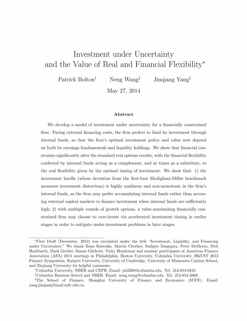
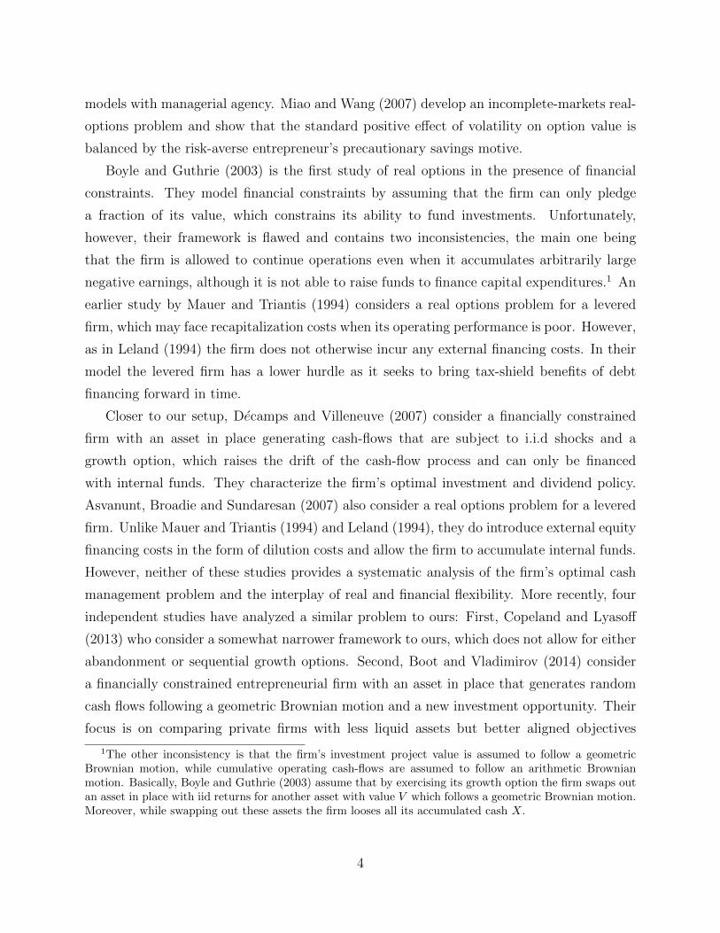
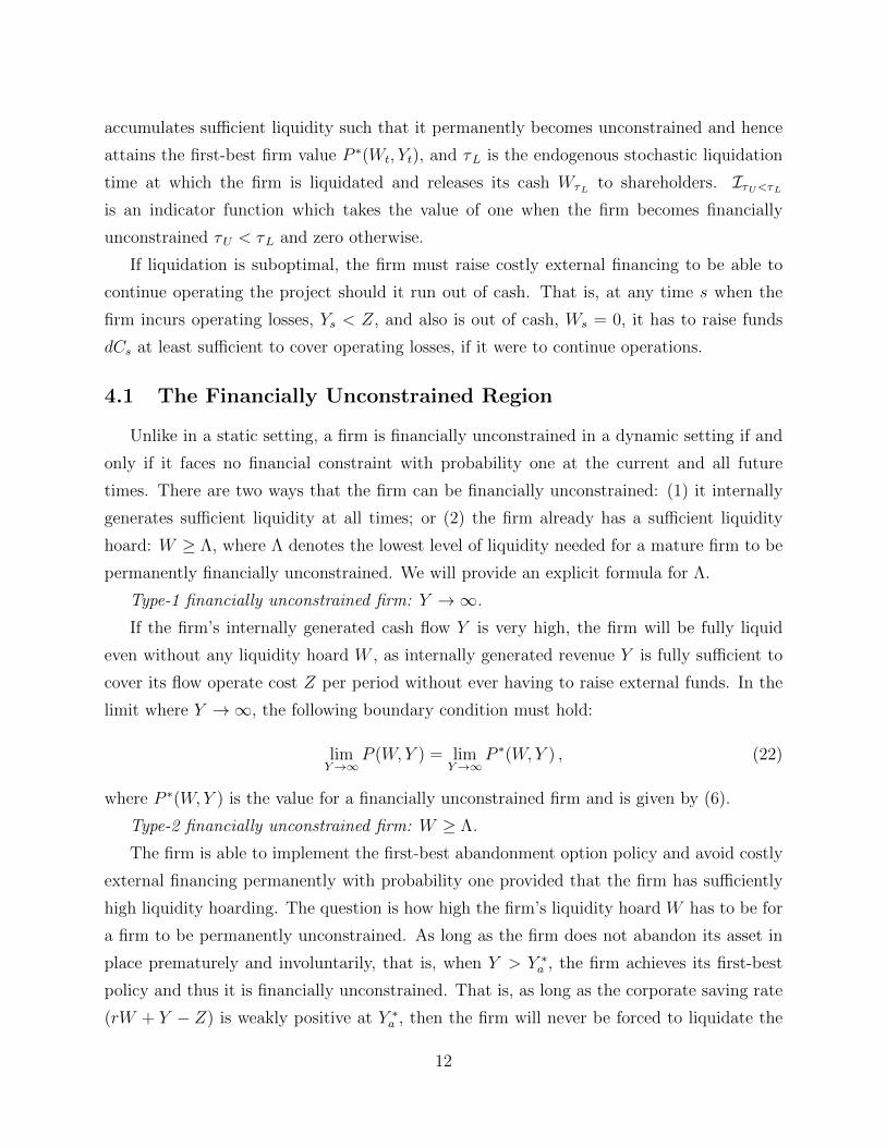
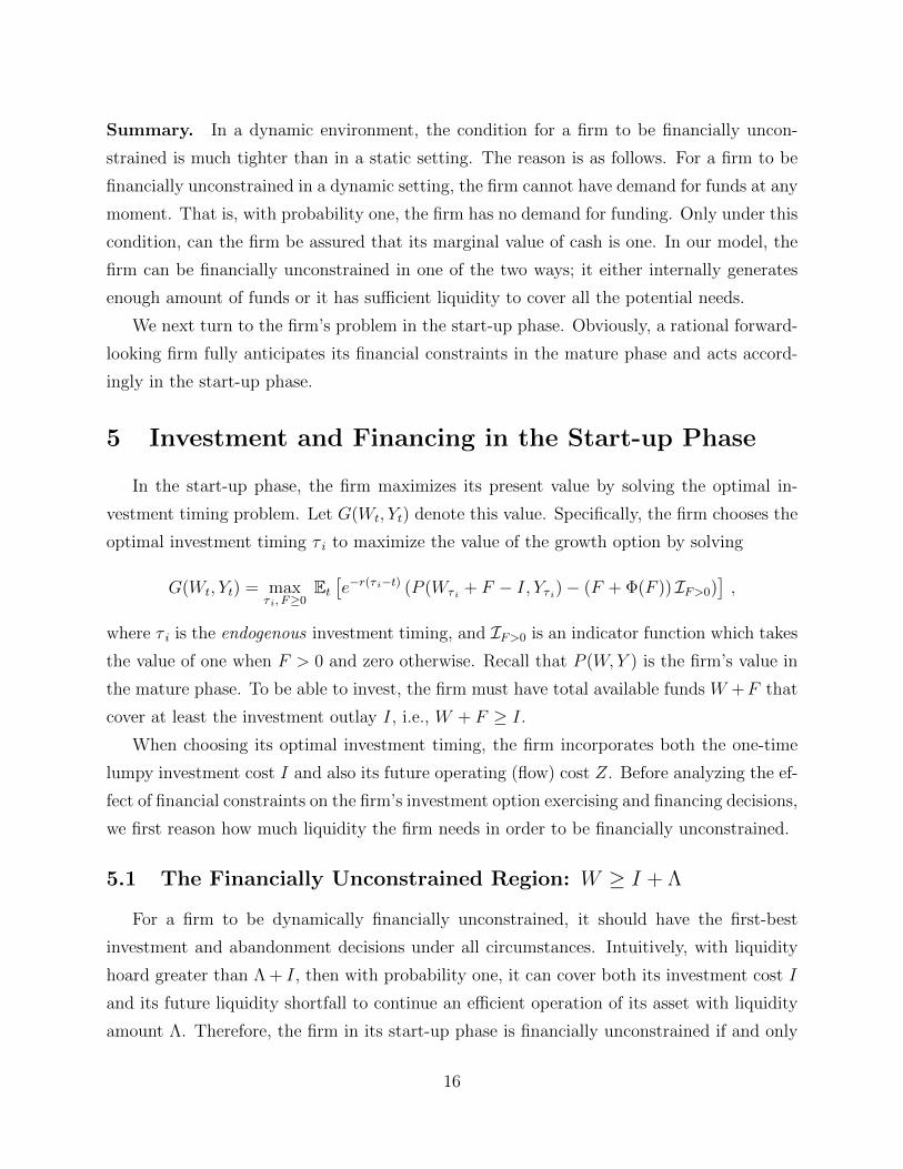
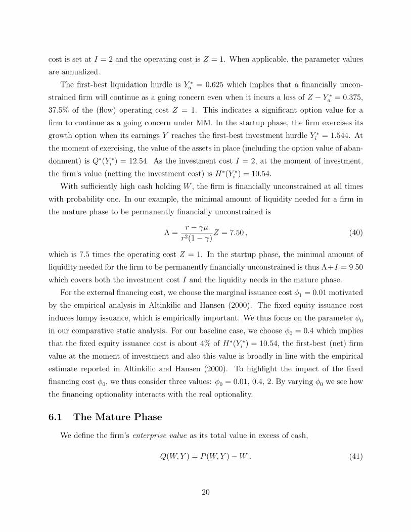
Figure 1: The optimal liquidation hurdle Y (W ) for a financially constrained firm inthe mature phase. The endogenous liquidation hurdle Y (W ) is monotonically decreasingwith liquidity holding W and approaches the first-best level Y ∗a = 0.625 independent of thefinancing cost φ0. For a given value of W , the larger the fixed equity issuance cost φ0,the higher the liquidation hurdle Y (W ) indicating a higher degree of under-investment. AtW = 0, Y (0) equals 0.645, 0.735, 0.895 for φ0 = 0.01, 0.4, 2, respectively.
Because cash is valuable beyond its face value for a financially constrained firm, the enterprise
value also depends on W . Under the MM condition, the enterprise value is independent of
the firm’s cash holding, and we have Q∗(Y ) = P ∗(W,Y )−W , as given by (6).
The Liquidation Decision. Figure 1 plots the optimal liquidation hurdle Y (W ) for a
financially constrained firm. First note that the firm becomes permanently financially un-
constrained when its cash holding reaches Λ = 7.50, which is 7.5 times the (annual) operating
cost Z = 1. For a financially unconstrained firm, it is optimal to liquidate its asset when
its earning Y falls below the first-best liquidation hurdle Y ∗a = 0.625. And importantly, the
firm will never be forced into sub-optimally abandoning its asset due to the shortage of its
liquidity W as long as W ≥ Λ = 7.50. Quantitatively, Figure 1 shows that the firm with
liquidity W larger than 3 is effectively dynamically financially unconstrained.
When the firm exhausts its internal funds Wτ = 0 and its cash flow is larger than its
operating cost Z (i.e., Y > Z = 1), the firm remains solvent purely relying on its internally
generated cash flow. However, when its earning Y falls below its operating cost (i.e., Y < 1),
it has to either raise external funds or will be liquidated otherwise. In our baseline case
21
where φ0 = 0.4, if a constrained firm’s earning Y lies in the region 1 > Y > Y (0) = 0.735,
it is optimal to issue equity keeping the firm alive. Only when its earnings Y falls below
0.735, the firm will abandon its asset rather than issue equity to finance its liquidity shortfall.
Recall that the first-best liquidation boundary is Y ∗a = 0.625. Hence, a firm with W = 0 will
be inefficiently liquidated due to lack of internal funds in the region 0.625 < Y ≤ 0.735.
Figure 1 also illustrates that the liquidation hurdle Y (W ) decreases with the firm’s liquid-
ity W in the region [0,Λ] = [0, 7.50] for all three levels of φ0. Hence, inefficiently liquidation
occurs in the region 0 ≤ W < Λ, as PW > 1 in this region and liquidity is valuable. For
example, when φ0 = 2, the abandonment hurdle decreases from Y (0) = 0.895 to Y ∗a = 0.625
as W increases from the origin to Λ = 7.50. Intuitively, the higher the liquidity hold-
ing W , the less inefficient the firm’s liquidation decision. For the case with a small fixed
equity issuance cost, φ0 = 0.01, the impact of financial constraints is negligible; the cash-
less firm will only be abandoned inefficiently if its earning Y falls inside the tight region
0.625 < Y ≤ Y (0) = 0.645. How important is the impact of financing costs on liquidation?
At the origin W = 0, as we increase the fixed issuance cost φ0 from 0.01 to 0.4 and then from
0.4 to 2, the abandonment hurdle Y (0) increases from 0.645 to 0.735 and then from 0.735
to 0.895, respectively. The implied real inefficiencies are significant. Finally, we note that
quantitatively the effect of financial constraints essentially disappears as the firm’s liquidity
hoard W reaches 1.6, even when the fixed equity issuance cost is relatively high, φ0 = 2.
The Equity Issuance Decision. The firm will consider the possibility of issuing equity
when it runs out of cash (W = 0) and its earning cannot cover its operating cost (Y < Z).
Intuitively, it is always preferable for the firm to postpone raising external funds whenever
feasible. Additionally, the firm will not issue equity if its earning falls below its first-best
abandonment hurdle Y ∗a , as it must be optimal for a financially constrained firm to abandon
its assets in place if it is optimal for a financially unconstrained firm to do so. Hence, in
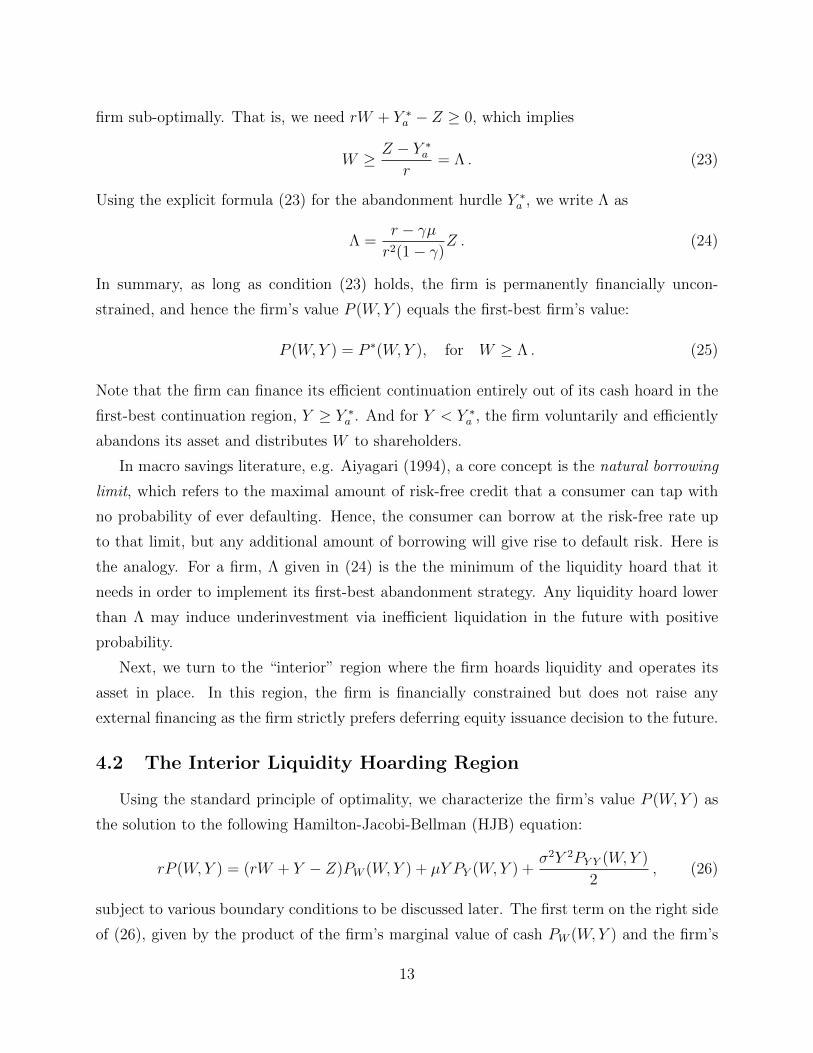
Figure 2, we only need to plot the optimal equity issuance amount Fa(Y ) as a function of
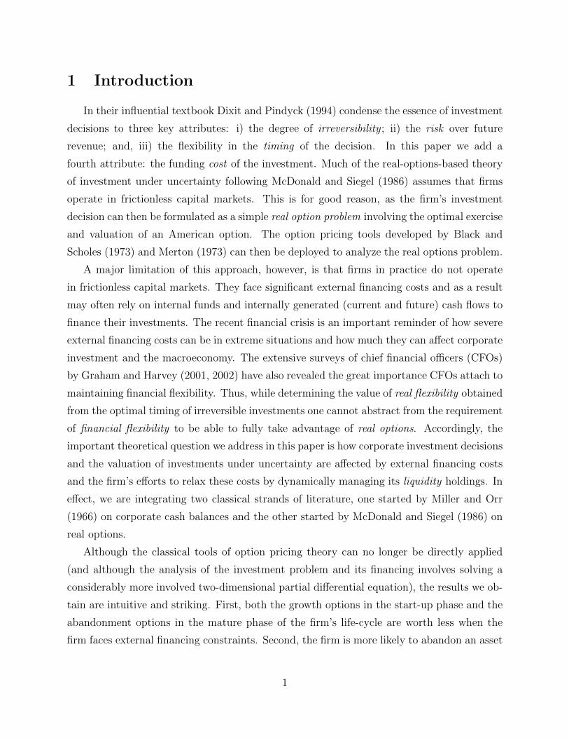
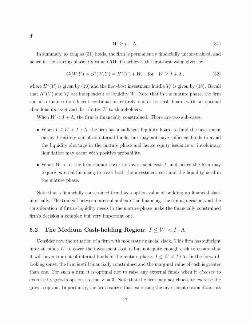
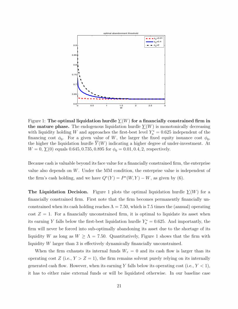
its earning Y in the region [Y ∗a , Z] = [0.625, 1] for the three cases, φ0 = 0.01, 0.4, 2.
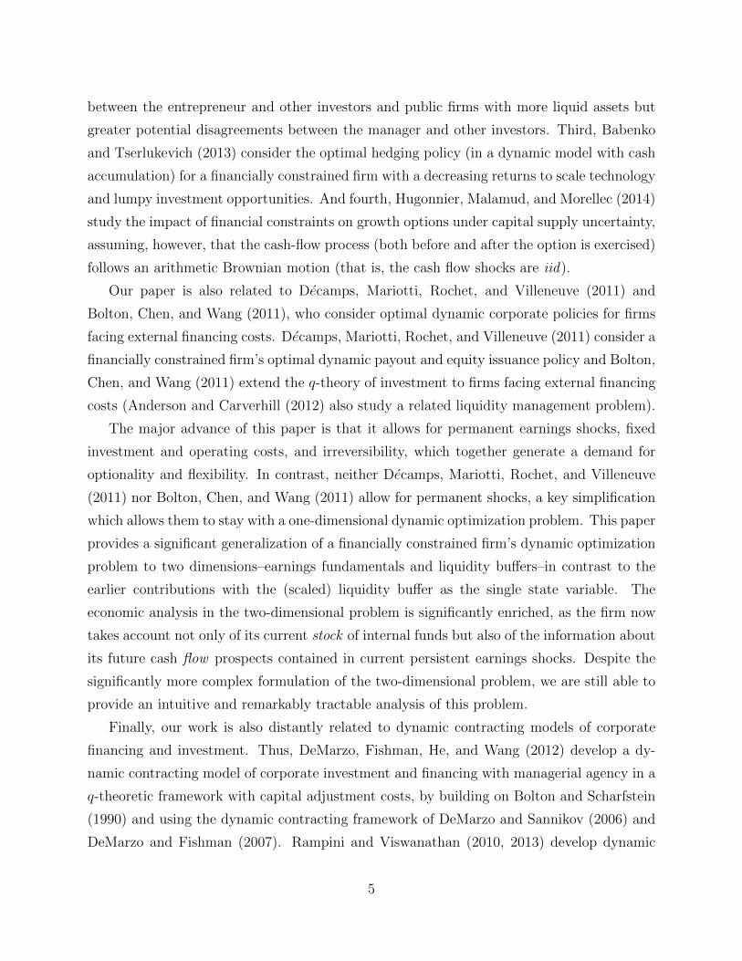
Importantly, the amount of equity financing Fa(Y ) may be non-monotonic in Y . For the
baseline case with φ0 = 0.4, Fa(Y ) first increases with Y in the region Y (0) < Y < 0.80
and then decreases with Y in the region 0.80 < Y < 1. The net issuance amount F peaks
at Y = 0.80 with a value of Fa(0.80) = 1.80. In the region 0.735 ≤ Y < 0.80, the firm’s
future prospects are not sufficiently encouraging for it to raise much external funding as
22
0.65 0.7 0.75 0.8 0.85 0.9 0.95 10
0.2
0.4
0.6
0.8
1
1.2
1.4
1.6
1.8
2
Y
optimal external financing Fa(Y)
q0=0.01q0=0.4q0=2
Figure 2: The optimal external financing Fa(Y ) for a financially constrained firmin the mature phase. Firms will choose to raise external funds only when it runs out of itsliquidity and when its internally generated cash flow cannot cover the operating cost Z but issufficiently high (i.e., only when W = 0 and Y (0) < Y < Z = 1), where Y (0) is the optimalabandonment hurdle for a financially constrained firm. For φ0 = 0.01, 0.4, 2, we have shownthat Y (0) = 0.645, 0.735, 0.895, respectively. Interestingly, the firm’s net financing amountFa(Y ) is non-monotonic in its earning Y over the region (Y (0), 1). For example, for the casewith φ0 = 0.4, the external financing Fa(Y ) first increases in the region Y ∈ (0.735, 0.80),peaks at Y = 0.80 with a value of Fa(0.80) = 1.80, and then decreases with Y in the regionY ∈ (0.80, 1).
23
the liquidation threat (in the future) is not low. This is the dominant consideration in this
region, so that when Y increases, it is marginally worth raising more funds (paying the
marginal cost φ1 = 0.01) given that the firm’s survival likelihood is improving. In the region
where Y ∈ (0.80, 1) on the other hand, the dominant consideration when Y increases is the
greater likelihood that the firm will be able to generate funds internally via its earning Y
and interest income rW in the near future so that the firm does not need much external
funds. As a result the firm optimally chooses to rely less on current external financing in the
expectation of larger future internally generated funds. Intuitively, the firm’s expectation
about its own future ability to generate internal funds (e.g., from operations and interest
incomes) significantly influences the firm’s current financing policy.
Additionally, conditional on choosing to raise funds, the firm raises more if the the fixed
costs of external funding φ0 are higher. For example, at Y = 0.9, as we increase the fixed
issuance cost φ0 from 0.01 to 0.4 and then from 0.4 to 2, the firm’s external financing Fa(0.9)
increases from 0.81 to 1.71, and then from 1.71 to 1.88. Intuitively, a firm that faces a larger
fixed issuance cost φ0 has a stronger incentive to issue more and hence capitalize on the
fixed cost φ0 as the cost of going back to the capital markets is greater in the future ceteris
paribus. Importantly, this prediction is the opposite to that based on the intuition from
static models such as Froot, Scharfstein, and Stein (1993) and Kaplan and Zingales (1997).
In these static models, the higher the financing cost, the more constrained the firm, and the
lower the amount of equity financing.
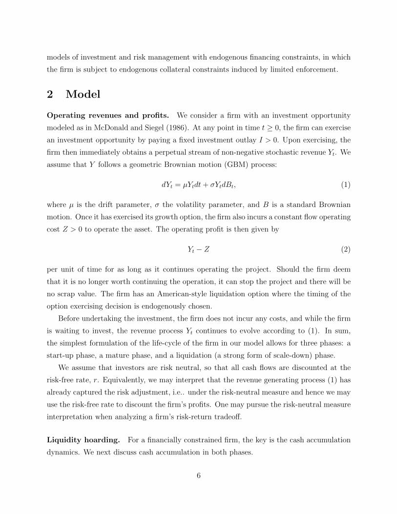
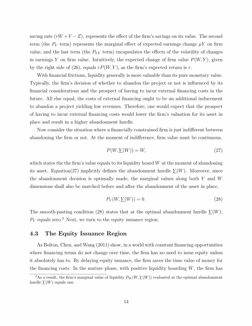
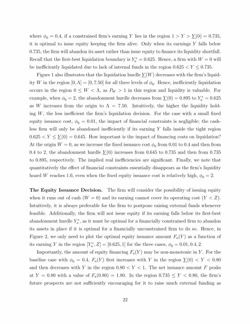
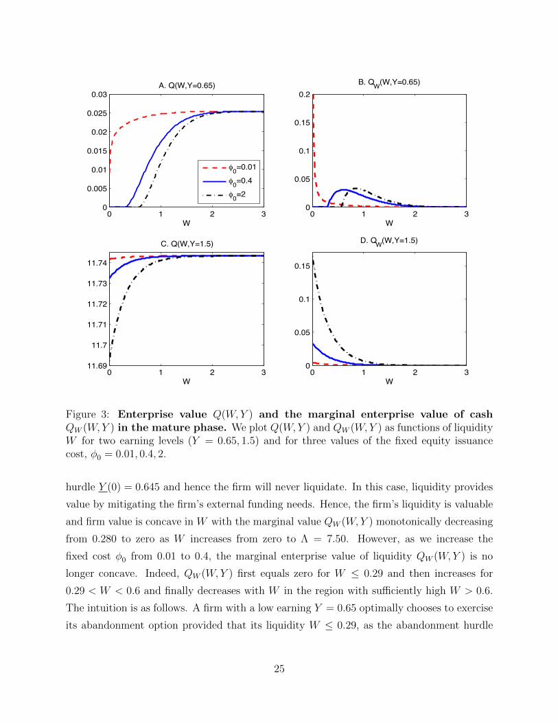
Figure 3 plots the firm’s enterprise value Q(W,Y ) and its marginal enterprise value of
cash QW (W,Y ) against liquidity W for two different levels of earning, Y = 0.65 and Y = 1.5,
and for three fixed equity issuance costs, φ0 = 0.01, 0.4, 2. Intuitively, the higher the financing
cost φ0, the lower the firm’s enterprise value Q(W,Y ). Also note that the net marginal value
of cash QW (W,Y ) is always positive implying that the firm is financially constrained and
hence liquidity is valuable in the constrained region, i.e., W < Λ = 7.50.
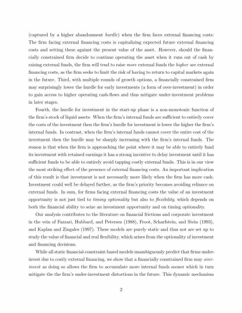
The firm’s value and the marginal value of liquidity. A central observation emerging
from Figure 3 is that the firm’s marginal enterprise value of cash QW (W,Y ) can vary non-
monotonically with its liquidity W . Panel B (with Y = 0.65) highlights the non-concavity
of Q(W,Y ) in W . Specifically, Q(W,Y ) can be either concave or convex in liquidity W .
First, consider the case with a small fixed equity issuance cost, φ0 = 0.01. Even with a
low earning, e.g., Y = 0.65, the firm will not abandon its asset as the firm’s abandonment
24
0 1 2 30
0.005
0.01
0.015
0.02
0.025
0.03
W
A. Q(W,Y=0.65)
0=0.01
0=0.4
0=2
0 1 2 311.69
11.7
11.71
11.72
11.73
11.74
W
C. Q(W,Y=1.5)
0 1 2 30
0.05
0.1
0.15
0.2
W
B. QW(W,Y=0.65)
0 1 2 30
0.05
0.1
0.15
W
D. QW(W,Y=1.5)
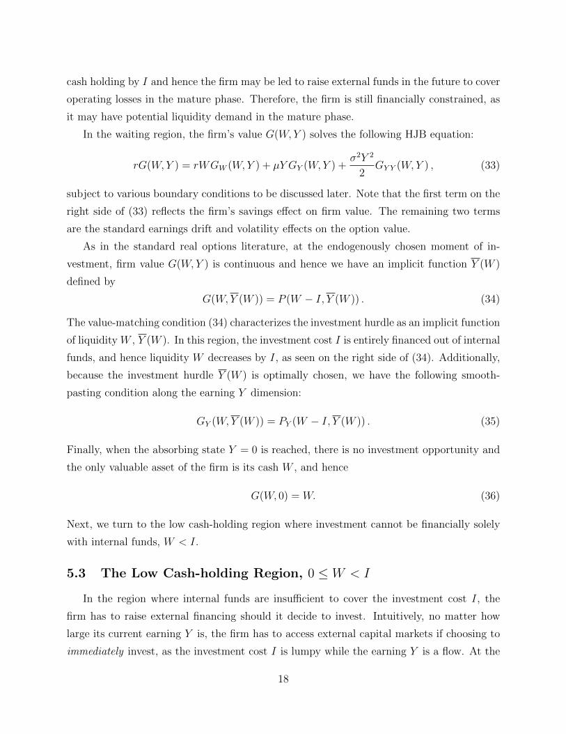
Figure 3: Enterprise value Q(W,Y ) and the marginal enterprise value of cashQW (W,Y ) in the mature phase. We plot Q(W,Y ) and QW (W,Y ) as functions of liquidityW for two earning levels (Y = 0.65, 1.5) and for three values of the fixed equity issuancecost, φ0 = 0.01, 0.4, 2.
hurdle Y (0) = 0.645 and hence the firm will never liquidate. In this case, liquidity provides
value by mitigating the firm’s external funding needs. Hence, the firm’s liquidity is valuable
and firm value is concave in W with the marginal value QW (W,Y ) monotonically decreasing
from 0.280 to zero as W increases from zero to Λ = 7.50. However, as we increase the
fixed cost φ0 from 0.01 to 0.4, the marginal enterprise value of liquidity QW (W,Y ) is no
longer concave. Indeed, QW (W,Y ) first equals zero for W ≤ 0.29 and then increases for
0.29 < W < 0.6 and finally decreases with W in the region with sufficiently high W > 0.6.
The intuition is as follows. A firm with a low earning Y = 0.65 optimally chooses to exercise
its abandonment option provided that its liquidity W ≤ 0.29, as the abandonment hurdle
25
Y (0.29) = 0.65. Hence, in the low liquidity region 0.29 < W < 0.6, increasing W lowers the
firm’s likelihood of tapping costly external financing, but the firm still has a low probability
to survive. In this case, the firm may be endogenously risk-loving with respect to exercising
its equity issuance option. This can only be the case if the firm faces strictly positive fixed
costs of equity issuance (φ0 > 0). And hence QW increases with W in this low-liquidity
region implying that firm value is locally convex in W in this region. Finally, when W > 0.6,
the firm has sufficiently high liquidity and equity issuance becomes much less likely causing
the marginal enterprise value of liquidity QW to decrease as the firm becomes less financially
constrained. We also see that with a higher φ0 (an increase of φ0 from 0.4 to 2) shifts
QW (W,Y ) as a function of W to the right while retaining the general non-monotonic shape.
This makes sense as a firm facing a larger external equity financing cost φ0 chooses a higher
abandonment hurdle Y (W ).
Now, we consider the case with a relative high earning, e.g., Y = 1.5, the firm’s enterprise
value Q(W,Y ) is now concave in W , as its earning is significantly larger than the abandon-
ment hurdle Y (W ) and the financing option is sufficiently deeply in the money. In these
cases, the firm behaves as it it were risk averse (PWW < 0) with respect to liquidity W .
6.2 The Start-up Phase
As for the mature phase, we again define the firm’s enterprise value in the start-up phase
as
H(W,Y ) = G(W,Y )−W . (42)
For a financially unconstrained firm, its enterprise value is independent of its cash holding,
i.e., H∗(Y ) = G∗(W,Y ) −W , and the closed-form solution for H∗(Y ) is given by (19). In
general, a financially constrained firm’s enterprise value depends on its cash holding W and
is lower than the first-best value, H(W,Y ) ≤ H∗(Y ) due to investment timing distortions.
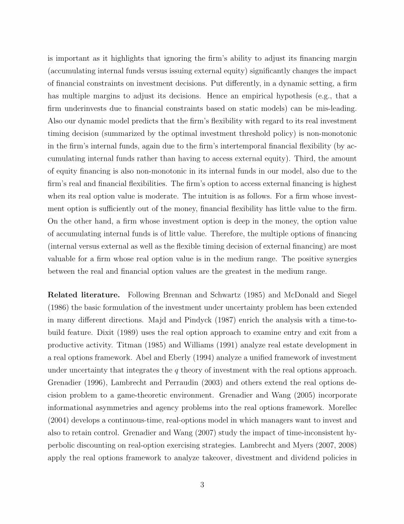
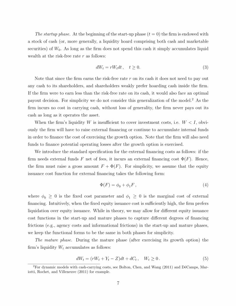
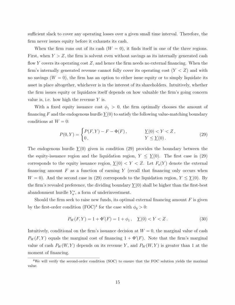
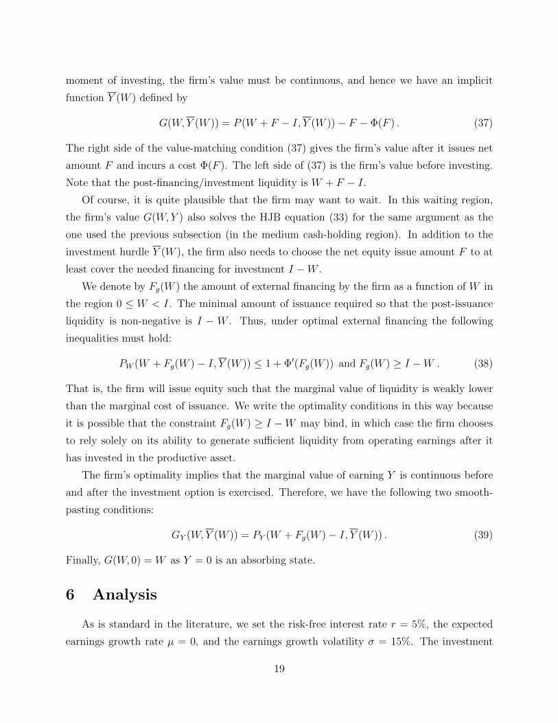
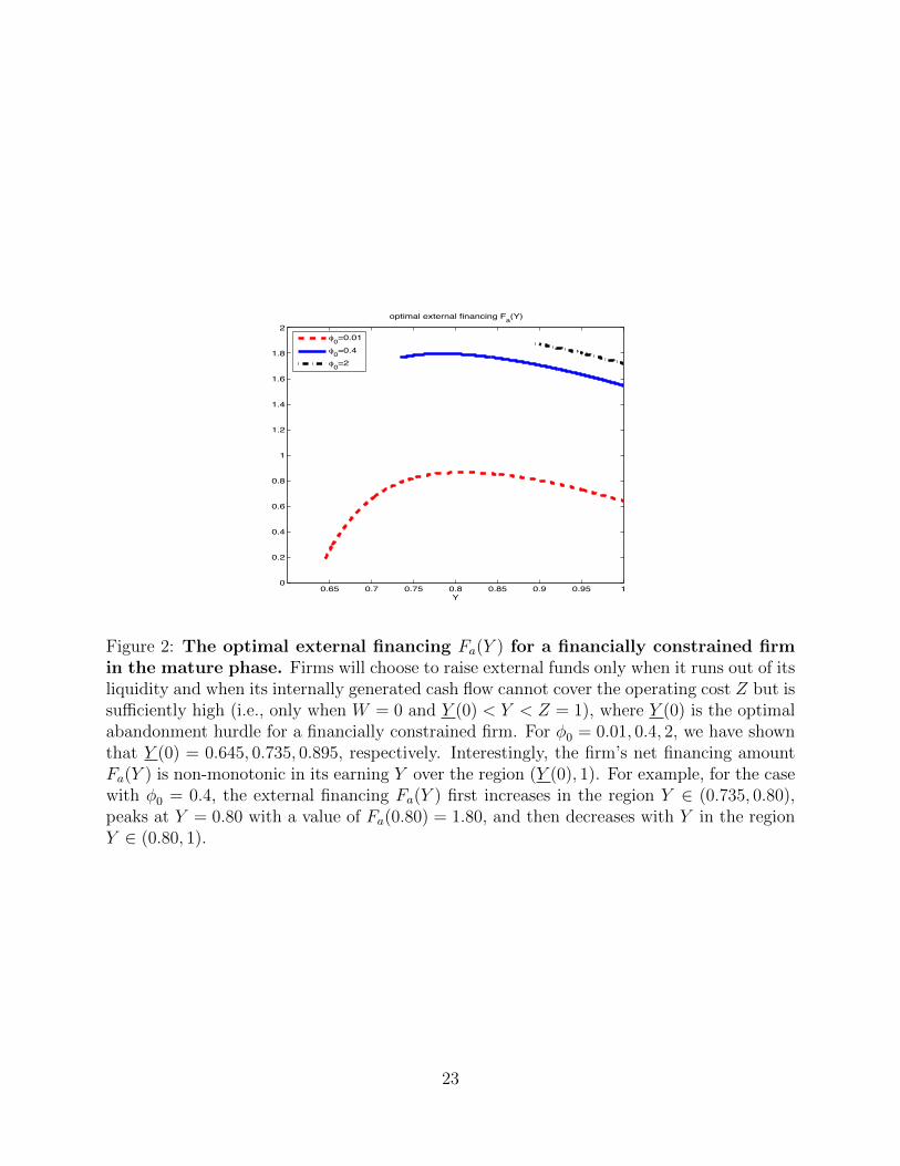
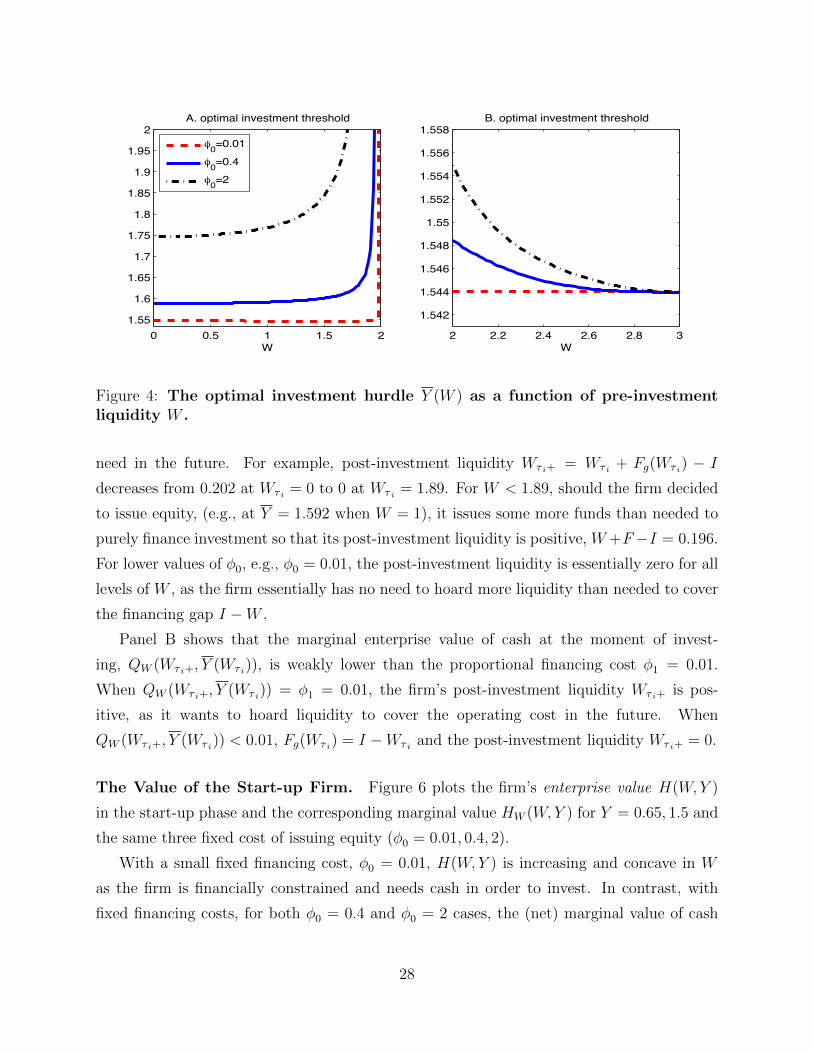
The Investment Decision. Figure 4 plots a financially constrained firm’s optimal in-
vestment hurdle Y (W ) for three values of the fixed cost, φ0 = 0.01, 0.4, 2. Recall that in
the start-up phase, a firm is financially unconstrained if its liquidity holding is greater than
I + Λ = 9.50. The firm pays the cost of I = 2 to exercise the investment option if and only
if the earning Y exceeds the endogenously chosen first-best time-invariant investment hurdle
Y ∗i = 1.544.
26
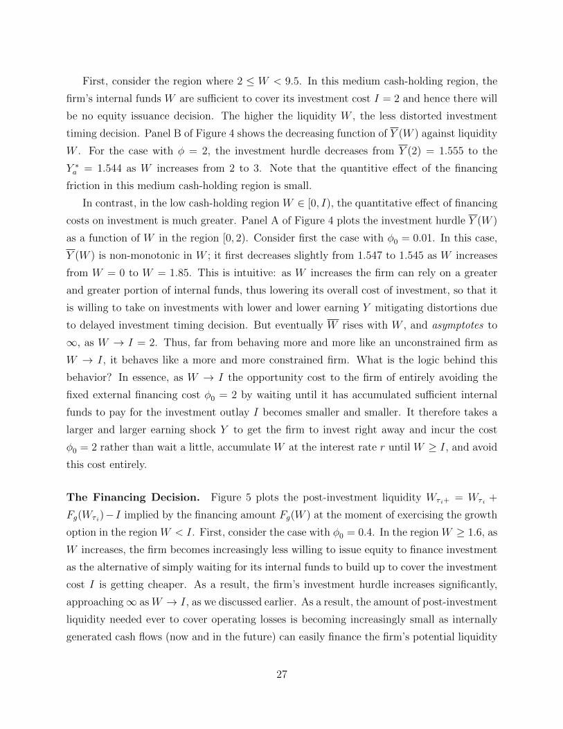
First, consider the region where 2 ≤ W < 9.5. In this medium cash-holding region, the
firm’s internal funds W are sufficient to cover its investment cost I = 2 and hence there will
be no equity issuance decision. The higher the liquidity W , the less distorted investment
timing decision. Panel B of Figure 4 shows the decreasing function of Y (W ) against liquidity
W . For the case with φ = 2, the investment hurdle decreases from Y (2) = 1.555 to the
Y ∗a = 1.544 as W increases from 2 to 3. Note that the quantitive effect of the financing
friction in this medium cash-holding region is small.
In contrast, in the low cash-holding region W ∈ [0, I), the quantitative effect of financing
costs on investment is much greater. Panel A of Figure 4 plots the investment hurdle Y (W )
as a function of W in the region [0, 2). Consider first the case with φ0 = 0.01. In this case,
Y (W ) is non-monotonic in W ; it first decreases slightly from 1.547 to 1.545 as W increases
from W = 0 to W = 1.85. This is intuitive: as W increases the firm can rely on a greater
and greater portion of internal funds, thus lowering its overall cost of investment, so that it
is willing to take on investments with lower and lower earning Y mitigating distortions due
to delayed investment timing decision. But eventually W rises with W , and asymptotes to
∞, as W → I = 2. Thus, far from behaving more and more like an unconstrained firm as
W → I, it behaves like a more and more constrained firm. What is the logic behind this
behavior? In essence, as W → I the opportunity cost to the firm of entirely avoiding the
fixed external financing cost φ0 = 2 by waiting until it has accumulated sufficient internal
funds to pay for the investment outlay I becomes smaller and smaller. It therefore takes a
larger and larger earning shock Y to get the firm to invest right away and incur the cost
φ0 = 2 rather than wait a little, accumulate W at the interest rate r until W ≥ I, and avoid
this cost entirely.
The Financing Decision. Figure 5 plots the post-investment liquidity Wτ i+ = Wτ i +
Fg(Wτ i)− I implied by the financing amount Fg(W ) at the moment of exercising the growth
option in the region W < I. First, consider the case with φ0 = 0.4. In the region W ≥ 1.6, as
W increases, the firm becomes increasingly less willing to issue equity to finance investment
as the alternative of simply waiting for its internal funds to build up to cover the investment
cost I is getting cheaper. As a result, the firm’s investment hurdle increases significantly,
approaching∞ asW → I, as we discussed earlier. As a result, the amount of post-investment
liquidity needed ever to cover operating losses is becoming increasingly small as internally
generated cash flows (now and in the future) can easily finance the firm’s potential liquidity
27
0 0.5 1 1.5 21.55
1.6
1.65
1.7
1.75
1.8
1.85
1.9
1.95
2
W
A. optimal investment threshold
q0=0.01q0=0.4q0=2
2 2.2 2.4 2.6 2.8 3
1.542
1.544
1.546
1.548
1.55
1.552
1.554
1.556
1.558
W
B. optimal investment threshold
Figure 4: The optimal investment hurdle Y (W ) as a function of pre-investmentliquidity W .
need in the future. For example, post-investment liquidity Wτ i+ = Wτ i + Fg(Wτ i) − I
decreases from 0.202 at Wτ i = 0 to 0 at Wτ i = 1.89. For W < 1.89, should the firm decided
to issue equity, (e.g., at Y = 1.592 when W = 1), it issues some more funds than needed to
purely finance investment so that its post-investment liquidity is positive, W+F−I = 0.196.
For lower values of φ0, e.g., φ0 = 0.01, the post-investment liquidity is essentially zero for all
levels of W , as the firm essentially has no need to hoard more liquidity than needed to cover
the financing gap I −W .
Panel B shows that the marginal enterprise value of cash at the moment of invest-
ing, QW (Wτ i+, Y (Wτ i)), is weakly lower than the proportional financing cost φ1 = 0.01.
When QW (Wτ i+, Y (Wτ i)) = φ1 = 0.01, the firm’s post-investment liquidity Wτ i+ is pos-
itive, as it wants to hoard liquidity to cover the operating cost in the future. When
QW (Wτ i+, Y (Wτ i)) < 0.01, Fg(Wτ i) = I −Wτ i and the post-investment liquidity Wτ i+ = 0.
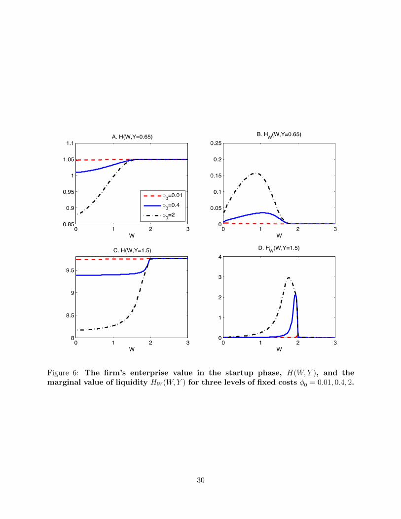
The Value of the Start-up Firm. Figure 6 plots the firm’s enterprise value H(W,Y )
in the start-up phase and the corresponding marginal value HW (W,Y ) for Y = 0.65, 1.5 and
the same three fixed cost of issuing equity (φ0 = 0.01, 0.4, 2).
With a small fixed financing cost, φ0 = 0.01, H(W,Y ) is increasing and concave in W
as the firm is financially constrained and needs cash in order to invest. In contrast, with
fixed financing costs, for both φ0 = 0.4 and φ0 = 2 cases, the (net) marginal value of cash
28

0 0.5 1 1.5 20.05
0
0.05
0.1
0.15
0.2
0.25
0.3
0.35
0.4
W
A. post investment liquidity W+F I
0=0.01
0=0.4
0=2
0 0.5 1 1.50
0.002
0.004
0.006
0.008
0.01
0.012B. Q_W(W+F I, \bar{Y}(W))
W2
Figure 5: Post-investment liquidity Wτ i+ = Wτ i + Fg(Wτ i)− I.
HW (W,Y ) first increases with W and then decreases with W as W becomes sufficiently
large. For example, consider the case with φ0 = 0.4 and Y = 0.65, HW (W, 0.65) is upward
sloping in W and reaches its highest value 0.035 around W = 1.05, and then declines as W
decreases, effectively approaching 0 as W exceeds 1.85.
Why is the firm’s growth option value H(W,Y ) convex in W in the region W < 1.05
for Y = 0.65? Intuitively, if the firm was able to take a mean-preserving spread with W
in that region, it would be better off, as either it accumulates internal funds faster or upon
incurring losses, the firm gets closer to issue external equity to finance the exercising of its
investment option. This additional benefit ameliorates the costly delay of the investment
exercising decision.
In contrast, in the region where W > 1.05, the financially constrained firm has sufficiently
high liquidity and hence has much weaker incentives to tap external financing and prefers
waiting until the time when it has accumulated sufficient internal funds to finance investment.
Therefore, the marginal value of cash HW (W,Y ) decreases with W in that region.
7 Simulation Illustration
To provide further insight into the dynamics of cash balances, financing, investment, and
abandonment decisions in our model, we simulate one sample path with two different initial
values for the firm’s cash holdings under our baseline parameter values. The implied time-
29
0 1 2 30.85
0.9
0.95
1
1.05
1.1
W
A. H(W,Y=0.65)
0=0.01
0=0.4
0=2
0 1 2 38
8.5
9
9.5
W
C. H(W,Y=1.5)
0 1 2 30
0.05
0.1
0.15
0.2
0.25
W
B. HW(W,Y=0.65)
0 1 2 30
1
2
3
4
W
D. HW(W,Y=1.5)
Figure 6: The firm’s enterprise value in the startup phase, H(W,Y ), and themarginal value of liquidity HW (W,Y ) for three levels of fixed costs φ0 = 0.01, 0.4, 2.
30
series of corporate decisions are illustrated in Figures 7 and 8 for the two cases, the first
with W0 = 1.8 and the second with W0 = 0.5. Table 1 also summarizes the implied equity
ownership dynamics that follow from the firm’s decisions over the simulated path used in
Figures 7 and 8.
In the Modigiani-Miller scenario where there are no external financing costs, the optimal
investment time for this sample path is t = 2.6, just when the firm’s earnings Yt reach 1.544,
and the abandonment time is t = 29.4, just as the firm’s earnings Yt hit the low level of
0.625. Thus, the firm is willing to fund losses of up to 37.5% of operating costs Z = 1 under
this scenario to maximize the value of its abandonment option.
Recall that when the firm incurs an external financing cost Φ(Ft) as it raises equity Ft
at time t, the firm’s post-issuance value is P (Wt+, Yt+). If we then denote the equilibrium
fraction of the newly issued equity held by outside investors by ωt+ we have:
ωt+ =Ft + Φ(Ft)
P (Wt+, Yt+)= 1− P (Wt, Yt)
P (Wt+, Yt+), (43)
given that the new investors just break even under perfectly competitive capital markets.
Under the simulated sample-path we can highlight the dynamics of equity dilution by keeping
track of the equity ownership of the original investors who have stayed with the firm since its
inception. We denote by αt the ownership share of the original equity holders at time t, with
α0 = 1 by construction. As the firm issues equity to finance investment and/or replenish
liquidity over time, the original equity investors’ ownership then evolves as follows:
αt+ = αt (1− ωt+) . (44)
In other words, with no issuance ωt+ = 0 and αt+ = αt, so that α does not change. But when
new equity is issued at time t, with a strictly positive ownership stake for new investors of
ωt+ > 0, the original equity investors’ equity is diluted to αt+ from αt according to (44).
Figure 7 plots the scenario where the firm starts with a high cash stock of W0 = 1.80.
Panel A plots the path of earnings Yt starting with Y0 = 1. Note first that when the firm
faces external financing costs it only exercises its investment option at time t = 2.9 when
Yt reaches 1.546 (compared with t = 2.6 when the firm faces no external financing costs).
It then pays the investment cost I = 2 solely out of internal funds, thus depleting its stock
of cash down to 0.08, as illustrated in Panel B. Given that the firm already starts out with
a relatively high cash stock of W0 = 1.8 it is optimal for the firm to wait until its internal
funds have accumulated sufficiently to be able to finance its investment cost entirely out of
internal funds, thus deferring costly external financing.
31
Next, at t = 7.5, when the firm’s earnings fall to 0.746 and it has burned through its
internal funds, the firm issues net equity of F (0.746) = 1.79 to replenish its liquidity Wt
from zero to 1.79, by selling 94.1% of its equity. At that point the firm’s original owners are
nearly wiped out and only retain a stake of 5.9%.
Finally, at t = 19.8, when the firm runs out cash for the second time and Yt reaches 0.656,
it simply abandons its asset and distributes the remaining cash of 0.07 to its shareholders.
At this low point the cost of new external financing simply outweighs the benefit of keeping
the firm as a going concern.
Figure 8 plots the scenario where the firm starts with a low cash stock of W0 = 0.5. Panel
A again plots the identical simulated path of earning Yt starting with Y0 = 1. When at t = 3.7
expected earnings Yt reach 1.592, the firm decides to raise net equity F (1.592) = 1.60 (see
Panel C) to finance its investment cost I = 2 via a combination of external equity (1.60)
and internal funds (0.40), leaving the firm with a stock of cash of 0.20 post-investment (as
shown in Panel B). As a result, the original owners are diluted down to an ownership stake
of only 85.3% (as shown in Panel D).
At t = 6.3, when earnings Yt have collapsed to 0.789 and the firm’s liquidity has been
drained, the firm returns to the capital markets and raises a net amount of F = 1.80, thus
further diluting the firm’s original owners’ down to 13.8% (see Panel D). Next, at t = 18.6,
as the firm’s liquidity Wt is again drained out, the firm yet again issues equity, raising a total
net amount of F = 1.73 and diluting the original owners down to a small stake of 5.7%.
Finally, at t = 28.6 the firm almost runs out of cash again and abandons its asset given that
expected operating earnings hit the low level of Yt = 0.692; it then distributes the remaining
cash 0.03 to its shareholders.
Comparing the two scenarios, we can make the following observations: First, in all cases
where the firm issues equity for purposes of replenishing its liquidity it chooses different
financing levels because each time it faces different expected operating earnings when it
exhausts its liquidity. Second, the firm with W0 = 1.8 turns out to abandon its asset sooner
(at t = 19.8) than the firm with W0 = 0.5 (at t = 28.6). This may at first appear surprising,
as one may think that a firm with more liquidity should have less distorted abandonment
decisions. The intuition for this seemingly counter-intuitive result is as follows. As it is
optimal for the firm with W0 = 1.8 to finance its investment cost I = 2 purely via internal
funds, this firm ends up with lower post-investment liquidity and hence an earlier inefficient
liquidation decision. Put differently, a less financially constrained firm could turn out to have
32
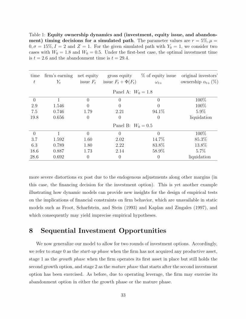
Table 1: Equity ownership dynamics and (investment, equity issue, and abandon-ment) timing decisions for a simulated path. The parameter values are r = 5%, µ =0, σ = 15%, I = 2 and Z = 1. For the given simulated path with Y0 = 1, we consider twocases with W0 = 1.8 and W0 = 0.5. Under the first-best case, the optimal investment timeis t = 2.6 and the abandonment time is t = 29.4.
time firm’s earning net equity gross equity % of equity issue original investors’
t Yt issue Ft issue Ft + Φ(Ft) ωt+ ownership αt+ (%)
Panel A: W0 = 1.8
0 1 0 0 0 100%2.9 1.546 0 0 0 100%7.5 0.746 1.79 2.21 94.1% 5.9%19.8 0.656 0 0 0 liquidation
Panel B: W0 = 0.5
0 1 0 0 0 100%3.7 1.592 1.60 2.02 14.7% 85.3%6.3 0.789 1.80 2.22 83.8% 13.8%18.6 0.887 1.73 2.14 58.9% 5.7%28.6 0.692 0 0 0 liquidation
more severe distortions ex post due to the endogenous adjustments along other margins (in
this case, the financing decision for the investment option). This is yet another example
illustrating how dynamic models can provide new insights for the design of empirical tests
on the implications of financial constraints on firm behavior, which are unavailable in static
models such as Froot, Scharfstein, and Stein (1993) and Kaplan and Zingales (1997), and
which consequently may yield imprecise empirical hypotheses.
8 Sequential Investment Opportunities
We now generalize our model to allow for two rounds of investment options. Accordingly,
we refer to stage 0 as the start-up phase when the firm has not acquired any productive asset,
stage 1 as the growth phase when the firm operates its first asset in place but still holds the
second growth option, and stage 2 as the mature phase that starts after the second investment
option has been exercised. As before, due to operating leverage, the firm may exercise its
abandonment option in either the growth phase or the mature phase.
33
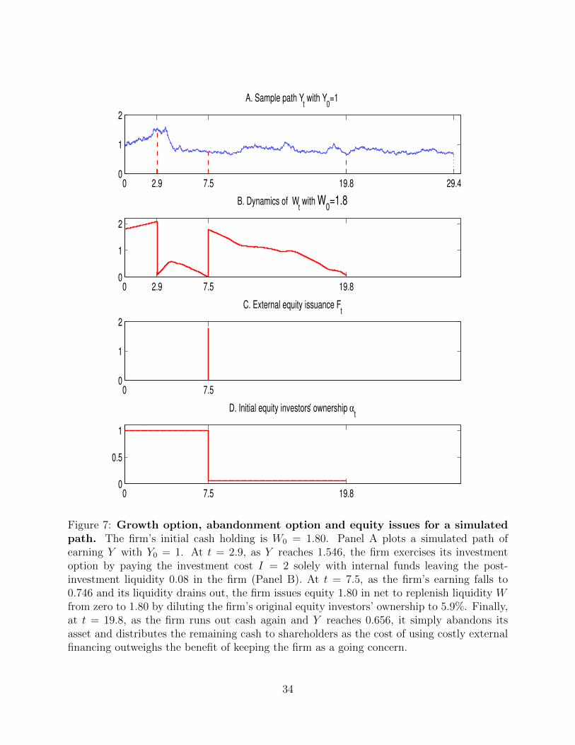
0 2.9 7.5 19.8 29.40
1
2
A. Sample path Yt with Y
0=1
0 2.9 7.5 19.80
1
2
B. Dynamics of Wt with W
0=1.8
0 7.50
1
2
C. External equity issuance Ft
0 7.5 19.80
0.5
1
D. Initial equity investors′ ownership αt
Figure 7: Growth option, abandonment option and equity issues for a simulatedpath. The firm’s initial cash holding is W0 = 1.80. Panel A plots a simulated path ofearning Y with Y0 = 1. At t = 2.9, as Y reaches 1.546, the firm exercises its investmentoption by paying the investment cost I = 2 solely with internal funds leaving the post-investment liquidity 0.08 in the firm (Panel B). At t = 7.5, as the firm’s earning falls to0.746 and its liquidity drains out, the firm issues equity 1.80 in net to replenish liquidity Wfrom zero to 1.80 by diluting the firm’s original equity investors’ ownership to 5.9%. Finally,at t = 19.8, as the firm runs out cash again and Y reaches 0.656, it simply abandons itsasset and distributes the remaining cash to shareholders as the cost of using costly externalfinancing outweighs the benefit of keeping the firm as a going concern.
34
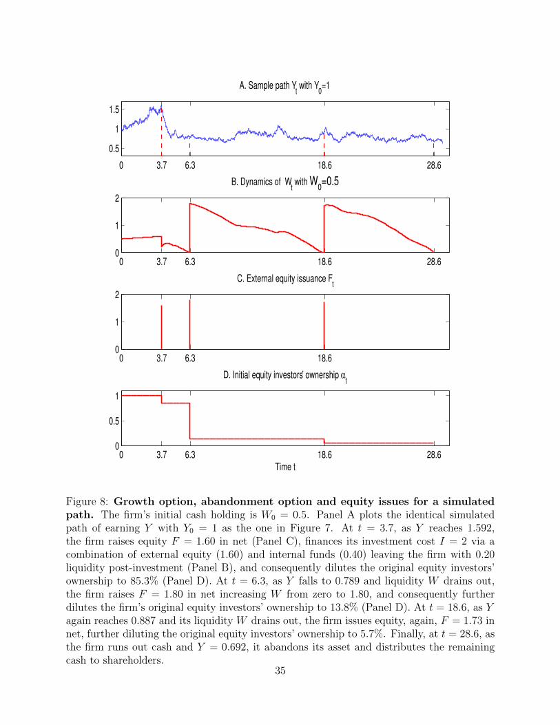
0 3.7 6.3 18.6 28.6
0.5
1
1.5
A. Sample path Yt with Y
0=1
0 3.7 6.3 18.6 28.60
1
2
B. Dynamics of Wt with W
0=0.5
0 3.7 6.3 18.60
1
2
C. External equity issuance Ft
0 3.7 6.3 18.6 28.60
0.5
1
D. Initial equity investors′ ownership αt
Time t
Figure 8: Growth option, abandonment option and equity issues for a simulatedpath. The firm’s initial cash holding is W0 = 0.5. Panel A plots the identical simulatedpath of earning Y with Y0 = 1 as the one in Figure 7. At t = 3.7, as Y reaches 1.592,the firm raises equity F = 1.60 in net (Panel C), finances its investment cost I = 2 via acombination of external equity (1.60) and internal funds (0.40) leaving the firm with 0.20liquidity post-investment (Panel B), and consequently dilutes the original equity investors’ownership to 85.3% (Panel D). At t = 6.3, as Y falls to 0.789 and liquidity W drains out,the firm raises F = 1.80 in net increasing W from zero to 1.80, and consequently furtherdilutes the firm’s original equity investors’ ownership to 13.8% (Panel D). At t = 18.6, as Yagain reaches 0.887 and its liquidity W drains out, the firm issues equity, again, F = 1.73 innet, further diluting the original equity investors’ ownership to 5.7%. Finally, at t = 28.6, asthe firm runs out cash and Y = 0.692, it abandons its asset and distributes the remainingcash to shareholders.
35
This extension allows us to analyze two novel effects. The first is the change in incentives
to exercise its first investment option caused by the prospect of acquiring valuable operating
cash-flows that help relax the internal funding constraint to finance the second growth option.
The second is how incentives to exercise the later investment option and other corporate
decisions are modified by operating cash-flow risk from the first productive asset.
A striking new result we obtain is that when the firm faces multiple rounds of growth
options it may choose to invest in the earlier opportunities sooner than under the first-best
benchmark. In other words, the firm optimally engages in a form of over-investment relative
to the first-best as a way of building up its liquidity which helps mitigate the incentives to
delay the second growth option. Accelerated timing of investment in the start-up phase may
be in the firm’s best interest if the cost of early investment in the initial productive asset
outweighs the costs of under-investment in the later expansion phase.
We denote by Zn the firm’s total operating cost (per unit of time) after exercising the
nth growth option, where n ∈ {1, 2}. Correspondingly, we denote the stochastic revenue
process generated by all existing productive assets by xnYt, where Yt is given in (1) and
where x1 < x2 denotes the production capacity after exercising respectively the first and
second investment option. That is, upon exercising the second growth option, the firm’s
operating revenue increases by ∆xY where ∆x = x2 − x1 and the operating cost increases
by ∆Z = Z2 − Z1. Intuitively, we may interpret ∆xY − ∆Z as the additional net revenue
generated by the second asset in place.
We also denote by τnL the abandonment time in phase n. In the growth phase, when the
firm exercises its abandonment option it releases its cash to shareholders and loses both its
first asset in place and its second growth option. In the mature phase the firm distributes
its cash to shareholders and liquidates all assets in place.
By backward induction, in the mature phase we essentially have the same firm value, the
same dynamics for liquidity, and the same abandonment decision as in the baseline model
when we replace the baseline cash flow with x2Y and the baseline operating cost with Z2.
The main changes to the analysis are thus in stages 0 and 1, to which we now turn. The
liquidity dynamics are the same as in the baseline model for the start-up phase and are given
in (3). As for stage 1, the growth phase, the firm’s liquidity Wt then accumulates as follows:
dWt = (rWt + x1Yt − Z1)dt+ dCt , Wt ≥ 0, (45)
where Ct denotes as before the undercounted cumulative equity issue and dC is the net
36
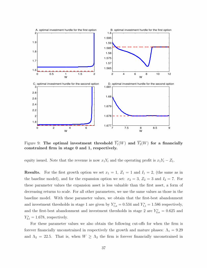
0 0.5 1 1.5 2
1.6
1.7
1.8
1.9
2
W
A. optimal investment hurdle for the first option
2 4 6 8 10 12
1.565
1.57
1.575
1.58
1.585
1.59
1.595
1.6
W
B. optimal investment hurdle for the first option
0 2 4 6
1.8
2
2.2
2.4
2.6
2.8
3
W
C. optimal investment hurdle for the second option
7 7.5 8 8.5 91.677
1.678
1.679
1.68
1.681
W
D. optimal investment hurdle for the second option
Figure 9: The optimal investment threshold Y1(W ) and Y2(W ) for a financiallyconstrained firm in stage 0 and 1, respectively.
equity issued. Note that the revenue is now x1Yt and the operating profit is x1Yt − Z1.
Results. For the first growth option we set x1 = 1, Z1 = 1 and I1 = 2, (the same as in
the baseline model), and for the expansion option we set: x2 = 3, Z2 = 3 and I2 = 7. For
these parameter values the expansion asset is less valuable than the first asset, a form of
decreasing returns to scale. For all other parameters, we use the same values as those in the
baseline model. With these parameter values, we obtain that the first-best abandonment
and investment thresholds in stage 1 are given by Y ∗1,a = 0.534 and Y ∗1,i = 1.586 respectively,
and the first-best abandonment and investment thresholds in stage 2 are Y ∗2,a = 0.625 and
Y ∗2,i = 1.678, respectively.
For these parameter values we also obtain the following cut-offs for when the firm is
forever financially unconstrained in respectively the growth and mature phases: Λ1 = 9.29
and Λ2 = 22.5. That is, when W ≥ Λ2 the firm is forever financially unconstrained in
37
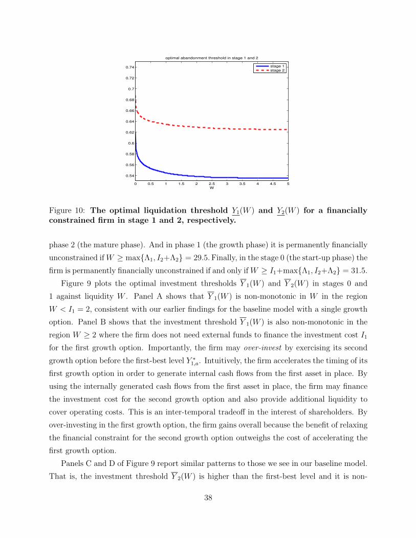
0 0.5 1 1.5 2 2.5 3 3.5 4 4.5 5
0.54
0.56
0.58
0.6
0.62
0.64
0.66
0.68
0.7
0.72
0.74
W
optimal abandonment threshold in stage 1 and 2
stage 1
stage 2
Figure 10: The optimal liquidation threshold Y1(W ) and Y2(W ) for a financiallyconstrained firm in stage 1 and 2, respectively.
phase 2 (the mature phase). And in phase 1 (the growth phase) it is permanently financially
unconstrained if W ≥ max{Λ1, I2+Λ2} = 29.5. Finally, in the stage 0 (the start-up phase) the
firm is permanently financially unconstrained if and only if W ≥ I1+max{Λ1, I2+Λ2} = 31.5.
Figure 9 plots the optimal investment thresholds Y 1(W ) and Y 2(W ) in stages 0 and
1 against liquidity W . Panel A shows that Y 1(W ) is non-monotonic in W in the region
W < I1 = 2, consistent with our earlier findings for the baseline model with a single growth
option. Panel B shows that the investment threshold Y 1(W ) is also non-monotonic in the
region W ≥ 2 where the firm does not need external funds to finance the investment cost I1
for the first growth option. Importantly, the firm may over-invest by exercising its second
growth option before the first-best level Y ∗1,a. Intuitively, the firm accelerates the timing of its
first growth option in order to generate internal cash flows from the first asset in place. By
using the internally generated cash flows from the first asset in place, the firm may finance
the investment cost for the second growth option and also provide additional liquidity to
cover operating costs. This is an inter-temporal tradeoff in the interest of shareholders. By
over-investing in the first growth option, the firm gains overall because the benefit of relaxing
the financial constraint for the second growth option outweighs the cost of accelerating the
first growth option.
Panels C and D of Figure 9 report similar patterns to those we see in our baseline model.
That is, the investment threshold Y 2(W ) is higher than the first-best level and it is non-
38
monotonic in the firm’s liquidity W .
Finally, we turn to Figure 10, which plots the firm’s abandonment thresholds Y1(W ) and
Y2(W ). Note that both abandonment thresholds decrease with liquidity and asymptotically
approach the first-best levels Y ∗1,a and Y ∗2,a, respectively. These results are consistent with
our earlier findings for the baseline model.
9 Conclusion
We develop a theory of real options for a financially constrained firm facing costly external
financing. We model the rich dynamic interactions between how a corporation manages its
real and financial flexibilities. Real options well capture the corporate flexibility on the
“real” side of corporate decision making (e.g., investment) and liquidity management is at
the core of corporate financial flexibility. Unlike in the standard MM framework, internal
funds significantly influence a financially constrained firm’s real investment and abandonment
option exercising decisions. Our analysis also brings out rich and subtle interactions between
the optimal investment and abandonment timing decisions and the firm’s sources of funds,
whether external, internal, or from current and future retained earnings. When the firm is
able to accumulate more internal funds it may well be induced to slow down its investment
even further as the prospect of being able to entirely avoid incurring external funding costs is
closer. Our framework is also sufficiently parsimonious to be able to provide quantitatively
plausible estimates of the value of the firm’s real options and its marginal value of cash, as
well as its optimal investment and external funding policy. Importantly, we find that with
multiple rounds of growth options, a financially constrained firm may over-invest in earlier
stages with the hope of replenishing liquidity in order to mitigate under-investment problems
in the future. We have, however, left other important features out of our analysis. We plan
to extend the framework by incorporating a credit line, risk management opportunities, and
capital structure margins as alternative sources of liquidity and risk management instruments
into our analysis.
39
Appendices
Before solving for the financially constrained firm’s value and optimal investment deci-
sions in the setting with multiple growth options, it is helpful to characterize the first-best
benchmark where the firm faces no external funding costs.
A The First-Best Benchmark
Let H∗(Y ) denote the solution for the first-best enterprise value in stage 0, Q∗n(Y ) the
solutions for the enterprise values in respectively stages n = 1, 2. Also, let Y ∗n,a and Y ∗n,i
denote the optimal abandonment boundaries and exercising thresholds of the nth growth
options in stages n = 1, 2, respectively.
We can then write Q∗1(Y ) as the solution to the following ODE:
rQ1(Y ) = (x1Y − Z1) + µY Q′1(Y ) +σ2Y 2
2Q′′1(Y ), (A.1)
subject to the following value-matching and smooth-pasting boundary conditions for the
investment and abandonment options:
Q1(Y∗2,i) = Q∗2(Y
∗2,i)− I2, (A.2)
Q′1(Y∗2,i) = Q∗′2 (Y ∗2,i), (A.3)
Q1(Y∗1,a) = 0, (A.4)
Q′1(Y∗1,a) = 0. (A.5)
Note that equation (A.1) for Q1(Y ) is identical to equation (7) for Q(Y ) except for the
first term, which reflects the fact that the firm is not operating at full scale and only has
one productive asset with capacity x1 and operating costs Z1. The upper boundary Y ∗2,i at
which the firm decides to scale up to full capacity is such that the growth-phase enterprise
value Q1(Y∗2,i) is just equal to the mature-phase enterprise value Q∗2(Y
∗2,i) net of investment
costs I2.
As we have established in Section 3.1, in the mature-phase, the firm’s value is given by
Q∗2(Y ;Z2) = Q∗(x2Y ;Z = Z2) and hence
Q∗2(Y ) =
(x2Y
r − µ− Z2
r
)+
(Y
Y ∗2,a
)γ (Z2
r−x2Y
∗2,a
r − µ
), for Y ≥ Y ∗2,a , (A.6)
40
where
Y ∗2,a =γ
γ − 1
r − µr
Z2
x2. (A.7)
After solving for Q∗2(Y ) we move backwards to the growth phase and solve for Q∗1(Y ).
As can be readily verified, the firm’s value Q∗1(Y ) in the region Y ∗2,i ≥ Y ≥ Y ∗1,a takes the
following form:
Q∗1(Y ) =
(x1Y
r − µ− Z1
r
)+ Ψi(Y )
(Q∗2(Y
∗2,i)− I2 +
Z1
r−x1Y
∗2,i
r − µ
)+ Ψa(Y )
(Z1
r−x1Y
∗1,a
r − µ
),
(A.8)
where
Ψi(Y ) =
(Y ∗β1,aY
γ − Y ∗γ1,aYβ
Y ∗β1,aY∗γ2,i − Y
∗γ1,aY
∗β2,i
)and Ψa(Y ) =
(Y ∗γ2,i Y
β − Y ∗β2,i Yγ
Y ∗β1,aY∗γ2,i − Y
∗γ1,aY
∗β2,i
), (A.9)
where β and γ are given by (20) and (12), the positive and negative roots of the fundamental
quadratic equation, and the first abandonment threshold Y ∗1,a and the second investment
threshold Y ∗2,i satisfy the boundary conditions (A.2)-(A.5).
Finally, we can move backwards to the start-up phase and solve for H∗(Y ), which satisfies
the ODE (15) and the boundary conditions:
H(Y ∗1,i) = Q∗1(Y∗1,i)− I1, (A.10)
H ′(Y ∗1,i) = Q∗′1 (Y ∗1,i). (A.11)
Again, it is straightforward to verify that H∗(Y ) takes the following form:
H∗(Y ) =
(Y
Y ∗1,i
)β (Q∗1(Y
∗1,i)− I1
)for Y ≤ Y ∗1,i , (A.12)
and Y ∗1,i solves the following implicit equation:
β[Q∗1(Y
∗1,i)− I1
]= Q∗′1 (Y ∗1,i)Y
∗1,i . (A.13)
B General Solution under External Financing Costs
In Section 4, we showed that a firm can be in one of three liquidity regions in the mature
phase: i) a financially unconstrained region (when W is sufficiently large or Y → ∞); ii)
an interior financially constrained region, and; iii) an equity issuance region. This naturally
continues to be the case for the mature phase in our more general setting.
41
B.1 The Mature Phase
The solution for the firm’s value in the mature phase, P (2)(W,Y ;Z2), is identical to
P (W,x2Y ;Z = Z2) given in Section 4. Note that the firm is permanently financially uncon-
strained in this region when its liquidity W ≥ Λ2 where Λ2 is given by
Λ2 ≡Z2 − x2Y ∗2,a
r≡ r − γµr2(1− γ)
Z2. (B.1)
The analysis is a bit more complicated but remains intuitive in the growth phase as the
firm has both a liquidation option and also the second growth option to exercise.
B.2 The Growth Phase
Again, the firm may be in one of these three regions in the growth phase (stage 1). Let
Λ1 denote the lowest level of liquidity such that the firm will not be inefficiently liquidated
in the growth phase. As long as the firm’s saving rate is positive at the first-best liquidation
threshold Y ∗1,a, which may be equivalently written as W ≥ Λ1, where
Λ1 ≡Z1 − x1Y ∗1,a
r, (B.2)
the firm will not be inefficiently liquidated in phase 1. However, for a firm to be permanently
financially unconstrained, it shall distort neither its liquidation decision nor its (second)
growth option exercising decision. For a firm to choose the first-best investment strategy for
the second growth option and to incur no further distortions, it needs at least an amount
of liquidity Λ2 + I2. This gives the following analytical characterization for the financially
unconstrained region.
The Unconstrained Region: When the firm neither satisfies
W ≥ max{Λ1, I2 + Λ2} (B.3)
or its revenues approaches infinity, i.e., Y → ∞, the firm will be permanently financially
unconstrained with probability one, and the value of the firm will be equal to the first-best
value: P (1)(W,Y ) = Q∗1(Y ) +W .
The Financially Constrained Region: When W < max{Λ1,Λ2 + I2}, the firm’s
value P (1)(W,Y ) satisfies the following HJB equation:
rP (1)(W,Y ) = (rW + x1Y1 − Z1)P(1)W (W,Y ) + µY P
(1)Y (W,Y ) +
σ2Y 2P(1)Y Y (W,Y )
2, (B.4)
42
subject to the following conditions:
P (1)(W,Y1(W )) = W, (B.5)
and
P(1)Y (W,Y1(W )) = 0. (B.6)
Intuitively, (B.5) states that the value of abandonment is simply equal to the firm’s cash
released to shareholders upon liquidation and (B.6) gives the smooth pasting condition for
the optimality of the endogenously chosen abandonment threshold Y1(W ). Additionally, the
firm’s value also satisfies the financing boundary condition at W = 0,
P (1)(0, Y ) =
{P (1)(F, Y )− F − Φ(F ) , Y1(0) < Y < Z1 ,
0 , Y ≤ Y1(0) ,(B.7)
where the optimal amount of funds raised F (net of issuing costs) is given by:
P(1)W (F, Y ) = 1 + Φ′(F ) = 1 + φ1 , Y1(0) < Y < Z1 . (B.8)
Finally, P (1)(W,Y ) also satisfies a set of boundary conditions that characterize the op-
timal growth option exercising decisions. Let F(2)g (W ) denote the amount of external funds
that the firm raises. Clearly, F(2)g (W ) ≥ I2 − W as W < I2. The additional conditions
needed to characterize the investment decisions are:
1. In the region I2 ≤ W < max{Λ1, I2 + Λ2}, the firm requires no external funds and in-
deed will not choose to tap external funds to finance its second growth option exercising
cost. Hence, we have the standard value-matching condition,
P (1)(W,Y 2(W )) = P (2)(W − I2, Y 2(W )) (B.9)
and the standard smooth-pasting condition,
P(1)Y (W,Y 2(W )) = P
(2)Y (W − I2, Y 2(W )) . (B.10)
2. In the region W < I2, at the growth option exercising boundary Y 2(W ), we have
P (1)(W,Y 2(W )) = P (2)(W + F (2)g (W )− I2, Y 2(W ))− F (2)
g (W )− Φ(F (2)g (W )) (B.11)
which is the standard value-matching condition, and
P(1)Y (W,Y 2(W )) = P
(2)Y (W + F (2)
g (W )− I2, Y 2(W )) , (B.12)
43
which is the standard smooth-pasting condition. Importantly, we pin down the amount
of financing F(2)g (W ) via the following conditions:
P(2)W (W + F (2)
g (W )− I2, Y 2(W )) ≤ 1 + Φ′(F (2)g (W )) and F (2)
g (W ) ≥ I2 −W . (B.13)
As in the baseline case, the constraint Fg(W ) ≥ I −W may bind as it may be optimal
for the firm to rely solely on its ability to generate sufficient liquidity from operating
earnings after it has exercised its second growth option. Note that the firm’s marginal
value of liquidity P(2)W (W + F
(2)g (W )− I2, Y 2(W )) cannot exceed the marginal cost of
financing at the moment of issuing equity to finance investment cost. Otherwise, the
firm should issue more and keep the proceeds inside the firm as retained earnings.
B.3 The Start-up Phase
We now characterize the solution for the start-up phase for the corresponding three
regions depending on the firm’s liquidity W . In the financially unconstrained region, where
W ≥ I1 + max{Λ1, I2 + Λ2} , (B.14)
we have the first-best solution for the firm’s option value:
G(W,Y ) = H∗(Y ) +W. (B.15)
In the financially constrained region where W < I1 + max{Λ1, I2 + Λ2} the firm’s value
G(W,Y ) solves the HJB equation:
rG(W,Y ) = rWGW (W,Y ) + µY GY (W,Y ) +σ2Y 2
2GY Y (W,Y ), (B.16)
subject to the following various boundary conditions. Let F(1)g (W ) denote the amount of
external funds that the firm raises. Clearly, F(1)g (W ) ≥ I1 −W as W < I1. The additional
conditions needed to characterize the investment decisions are:
1. In the region I1 ≤ W < I1 + max{Λ1, I2 + Λ2}, the firm issues no equity to finance the
exercising cost of the first growth option. We have the standard value-matching and
smooth-pasting conditions:
G(W,Y1(W )) = P (1)(W − I1, Y1(W )) , (B.17)
GY (W,Y1(W )) = P(1)Y (W − I1, Y1(W )). (B.18)
44
2. In the region 0 ≤ W < I1, the firm has to raise external financing, denoted by F(1)g (W ),
if it wants to exercise its first growth option. We thus have the following value-matching
and smooth-pasting conditions:
G(W,Y1(W )) = P (1)(W + F (1)g (W )− I1, Y1(W ))− F (1)
g (W )− Φ(F (1)g (W )) , (B.19)
GY (W,Y1(W )) = P(1)Y (W + F (1)
g (W )− I1, Y1(W )), (B.20)
To pin down the external financing amount, F(1)g (W ), we use the following conditions:
P(1)W (W + F (1)
g (W )− I1, Y 1(W )) ≤ 1 + Φ′(F (1)g (W )) and F (1)
g (W ) ≥ I1 −W . (B.21)
The argument for the optimality condition (B.21) for F(1)g (W ) is essentially the same as the
optimality condition (B.13) for F(2)g (W ). Finally, G(W,Y ) also satisfies the absorbing barrier
condition G(W, 0) = W .
We have now completely characterized the HJB equations and various boundary con-
ditions in the three phases of the firm. We next numerically solve the model and provide
intuitive explanations for our model’s main results.
45
References
Abel, A.B., and J.C. Eberly, 1994. A unified model of investment under uncertainty.
American Economic Review 84, 1369–1384.
Aiyagari, S. R., 1994. Uninsured idiosyncratic risk and aggregate saving. Quarterly Journal
of Economics 99, 659–684.
Altinkilic, O., and R.S. Hansen, 2000. Are there economies of scale in underwriting fees?
Evidence of rising external financing costs. Review of Financial Studies 13, 191–218.
Anderson, R., and A. Carverhill, 2012. Corporate Liquidity and Capital Structure. Review
of Financial Studies 20, 1429-1460.
Asvanunt, A., M. Broadie, and S. Sundaresan, 2007. Growth Options and Optimal Default
under Liquidity Constraints: The Role of Corporate Cash Balances. Columbia Business
School Research Paper.
Babenko I., and Y. Tserlukevich, 2013. Embracing Risk: Hedging Policy for Firms with
Real Options, working paper, Arizona State University.
Black, F., and M. Scholes, 1973. The pricing of options and corporate liabilities. Journal
of Political Economy 81, 637–659.
Bolton, P., H. Chen, and N. Wang, 2011. A unified theory of Tobin’q, corporate investment,
financing, and risk management. Journal of Finance 66, 1545–1578.
Bolton, P., and D. Scharfstein, 1990. A theory of predation based on agency problems in
financial contracting. American Economic Review 80, 93–106.
Boot, A.W.A., and V. N. Vladimirov, 2014. Entrepreneurial Vision, Information, and Cash.
Working paper. University of Amsterdam.
Boyle, G., and G. Guthrie, 2003. Investment, Uncertainty, and Liquidity. Journal of
Finance 58, 2143–2166.
Brennan, M.J., and E. Schwartz, 1985. Evaluating natural resource investments. Journal
of Business 58, 135–157.
46
Copeland, T., and A. Lyasoff, 2013. Seeking q: the Marginal Efficiency of Liquidity and
its Effect on Investment Financing and Valuation. Working paper. University of San
Diego and Boston University.
DeCamps, J.P., T. Mariotti, J.C. Rochet, and S. Villeneuve, 2011. Free cash flow, issuance
costs and stock prices. Journal of Finance 66, 1501–1544.
DeCamps, J.P., and S. Villeneuve, 2007. Optimal dividend policy and growth option.
Finance and Stochastics 11, 3–27.
DeMarzo, P.M., M.J. Fishman, Z. He, and N. Wang, 2012. Dynamic agency and the q
theory of investment. Journal of Finance 67, 2295–2340.
DeMarzo, P.M., and Y. Sannikov, 2006. Optimal security design and dynamic capital
structure in a continuous–time agency model. Journal of Finance 61, 2681-2724.
DeMarzo, P.M., and M.J. Fishman, 2007. Optimal long-term financial contracting. Review
of Financial Studies 20, 2079–2128.
Dixit, A.K., 1989. Entry and exit decisions under uncertainty. Journal of Political Economy
97, 620–638.
Dixit, A.K., and R.S. Pindyck, 1994. Investment Under Uncertainty. Princeton University
Press, Princeton, NJ.
Fazzari, S., G.R. Hubbard, and B. Petersen, 1988. Finance constraints and corporate
investment. Brookings Papers on Economic Activity 1, 141–195.
Froot, K.A., D.S. Scharfstein, and J.C. Stein, 1993. Risk Management: Coordinating
Corporate Investment and Financing Policies. The Journal of Finance 48, 1629–1658.
Goldstein, R., Ju, N., and H. Leland, 2001. An EBIT-based model of dynamic capital
structure, Journal of Finance 74, 483–512.
Graham, J.R., and C. Harvey, 2001. The Theory and Practice of Corporate Finance:
Evidence from the Field. Journal of Financial Economics 60, 187–243.
Graham, J.R., and C. Harvey, 2002. How Do CFOs Make Capital Budgeting and Capital
Structure Decisions?. Journal of Applied Corporate Finance 15, 8–23.
47
Grenadier, S.R., 1996. The strategic exercise of options: development cascades and over-
building in real estate markets. Journal of Finance 51, 1653–1679.
Grenadier, S.R., and N. Wang, 2005. Investment timing, agency, and information. Journal
of Financial Economics 75, 493–533.
Grenadier, S.R., and N. Wang, 2007. Investment under uncertainty and time-inconsistent
preferences. Journal of Financial Economics 84, 2-39.
Hugonnier, J., S. Malamud, and E. Morellec, 2014. Capital supply uncertainty, cash hold-
ings, and investment. Working paper. Swiss Finance Institute.
Kaplan, S.N., and L. Zingales, 1997. Do investment-cash flow sensitivities provide useful
measures of financing constraints? Quarterly Journal of Economics 112, 169–215.
Lambrecht, B.M., and W.R. Perraudin, 2003. Real options and preemption under incom-
plete information. Journal of Economic Dynamics and Control 27, 619–643.
Lambrecht, B.M., and S. C. Myers, 2007. A theory of takeovers and disinvestment. Journal
of Finance. 62, 809–845.
Lambrecht, B.M., and S. C. Myers, 2008. Debt and managerial rents in a real-options
model of the firm. Journal of Financial Economics 89, 209–231.
Leland, H. E., 1994. Corporate debt value, bond covenants, and optimal capital structure.
Journal of Finance 49, 1213-1252.
Majd, S., and R. Pindyck, 1987. Time to build, option value, and investment decision.
Journal of Financial Economics 18, 7–28.
Mauer, D., and A.J. Triantis, 1994. Interactions of Corporate Financing and Investment
Decisions: A Dynamic Framework. Journal of Finance 49, 1253–1277.
McDonald, R., and D. Siegel, 1986. The value of waiting to invest. Quarterly Journal of
Economics 101, 707–727.
Merton, R.C., 1973. Theory of rational option pricing. Bell Journal of Economics and
Management Science 4, 141–183.
48
Miao, J., and N. Wang, 2007. Investment, consumption, and hedging under incomplete
markets. Journal of Financial Economics 86, 608–642.
Miller, M. H., and D. Orr, 1966. A model of demand for money by firms. Quarterly Journal
of Economics 80, 413–435.
Morellec, E., 2004. Can managerial discretion explain observed leverage ratios?. Review of
Financial Studies 17, 257–294.
Rampini, A.A., and S. Viswanathan, 2010. Collateral, risk management, and the distribu-
tion of debt capacity. Journal of Finance 65, 2293–2322.
Rampini, A.A., and S. Viswanathan, 2013. Collateral and capital structure. Journal of
Financial Economics 109, 466–492.
Titman, S., 1985. Urban land prices under uncertainty. American Economic Review 75,
505–514.
Williams, J.T., 1991. Real estate development as an option. Journal of Real Estate Finance
and Economics 4, 191–208.
49