Investment Analysis and Portfolio management

Lecture: 24

Course Code: MBF702

Outline

• RECAP• Portfolio returns• Portfolio proportion• Mean or Average return• Variance and covariance• Sample covariance• Expectations• Expected returns• Population variance• Population covariance

Portfolio Return

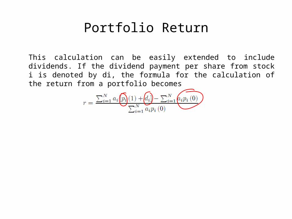
This calculation can be easily extended to include dividends. If the dividend payment per share from stock i is denoted by di, the formula for the calculation of the return from a portfolio becomes

Portfolio Return

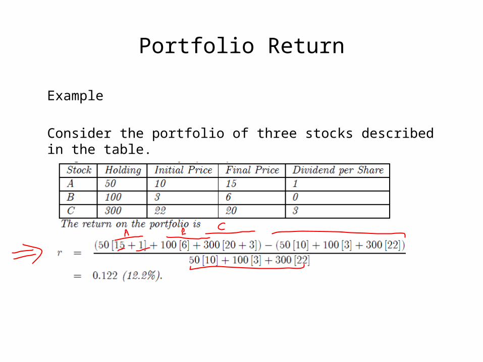
Example

Consider the portfolio of three stocks described in the table.

Portfolio Return

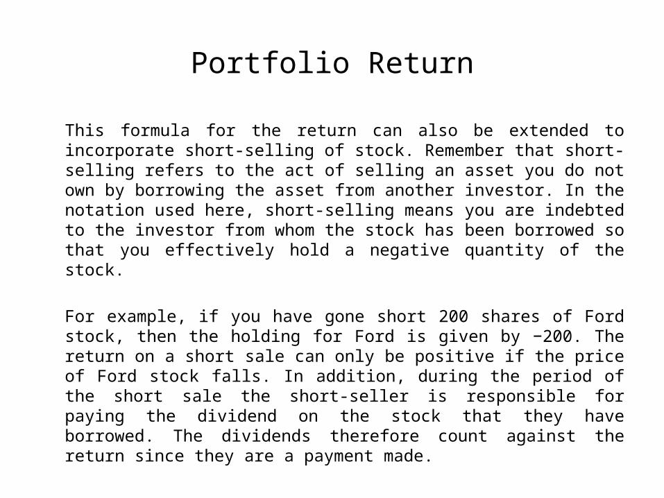
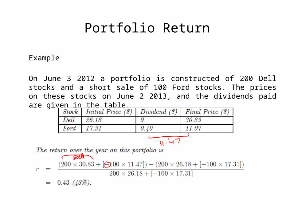
This formula for the return can also be extended to incorporate short-selling of stock. Remember that short-selling refers to the act of selling an asset you do not own by borrowing the asset from another investor. In the notation used here, short-selling means you are indebted to the investor from whom the stock has been borrowed so that you effectively hold a negative quantity of the stock.

For example, if you have gone short 200 shares of Ford stock, then the holding for Ford is given by −200. The return on a short sale can only be positive if the price of Ford stock falls. In addition, during the period of the short sale the short-seller is responsible for paying the dividend on the stock that they have borrowed. The dividends therefore count against the return since they are a payment made.

Portfolio Return

Example

On June 3 2012 a portfolio is constructed of 200 Dell stocks and a short sale of 100 Ford stocks. The prices on these stocks on June 2 2013, and the dividends paid are given in the table.

Portfolio proportions

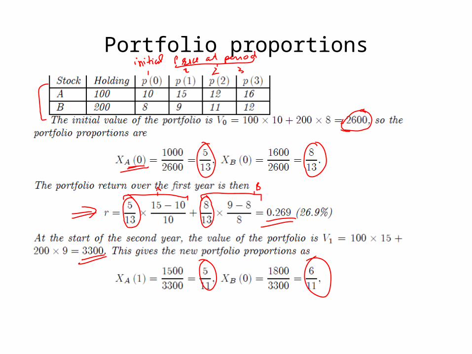
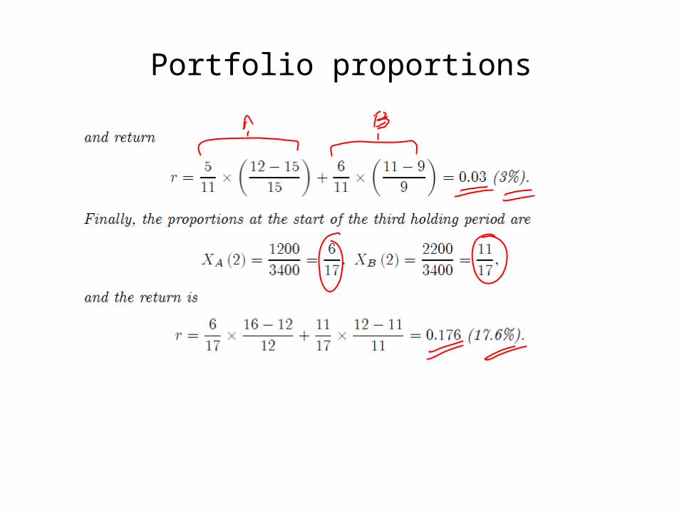
The calculations of portfolio return so far have used the quantity held of each asset to determine the initial and final portfolio values. What proves more convenient in later calculations is to use the proportion of the portfolio invested in each asset rather then the total holding. The two give the same answer but using proportions helps emphasize that the returns (and the risks discussed later) depend on the mix of assets held, not on the size of the total portfolio.

Example

A portfolio consists of two stocks, neither of which pays any dividends. The prices of the stock over a three year period and the holding of each is given in the table.

Portfolio proportions

Portfolio proportions

Mean or Average return

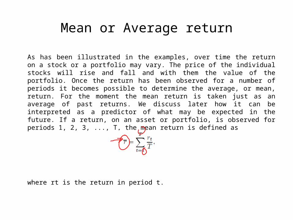
As has been illustrated in the examples, over time the return on a stock or a portfolio may vary. The price of the individual stocks will rise and fall and with them the value of the portfolio. Once the return has been observed for a number of periods it becomes possible to determine the average, or mean, return. For the moment the mean return is taken just as an average of past returns. We discuss later how it can be interpreted as a predictor of what may be expected in the future. If a return, on an asset or portfolio, is observed for periods 1, 2, 3, ..., T, the mean return is defined as

where rt is the return in period t.

Mean or Average return

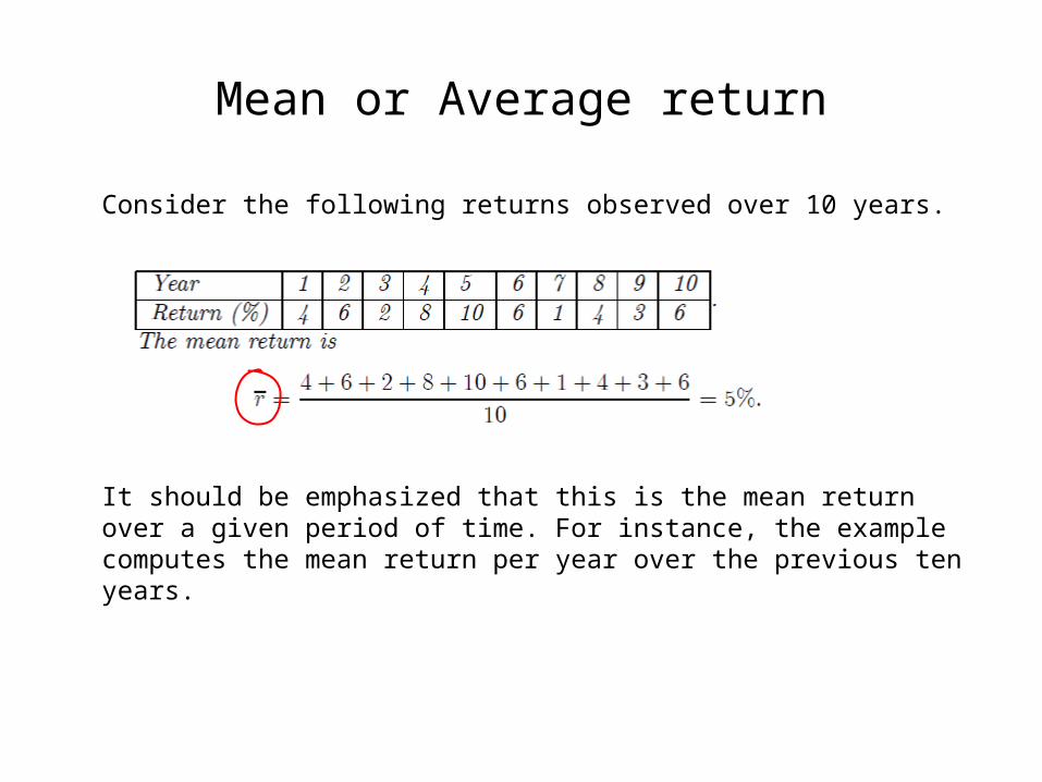
Consider the following returns observed over 10 years.

It should be emphasized that this is the mean return over a given period of time. For instance, the example computes the mean return per year over the previous ten years.

Variance and Covariance

It has already been stressed that as well as the return on the portfolio, the investor has to be concerned with the risk. What risk means in this context is the extent to which the return varies over time. Two assets may have an identical mean return but very different degrees of risk. The standard measure of risk used in investment analysis is the variance of return (or, equivalently, its square root which is called the standard deviation).

When constructing a portfolio it is not just the risk on individual assets that matters but also the way in which this risk combines across assets to give the portfolio variance. Two assets may be individually risky but if these risks cancel then a portfolio of the two may have very little risk. The risks will cancel if a higher than average return on one of the assets always accompanies a lower than average return on the other. The measure of the way returns are related across assets is called the covariance of return. The covariance will be seen to be central to understanding portfolio construction.

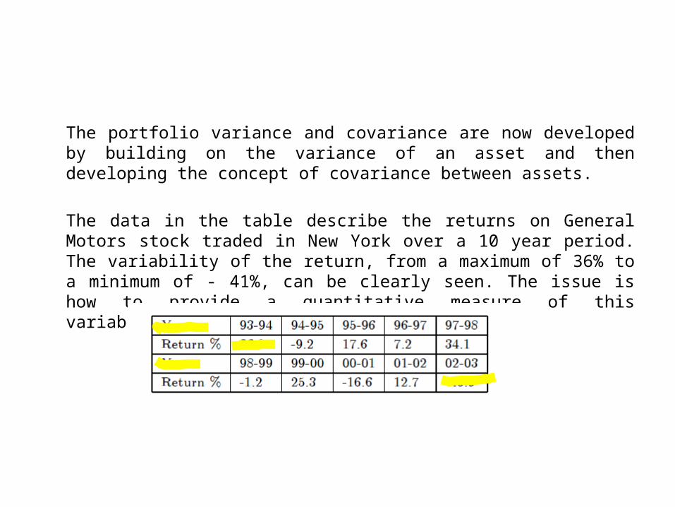
The portfolio variance and covariance are now developed by building on the variance of an asset and then developing the concept of covariance between assets.

The data in the table describe the returns on General Motors stock traded in New York over a 10 year period. The variability of the return, from a maximum of 36% to a minimum of - 41%, can be clearly seen. The issue is how to provide a quantitative measure of this variability.

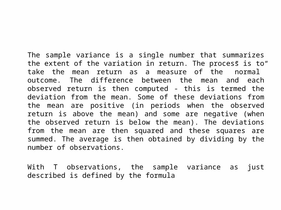
The sample variance is a single number that summarizes the extent of the variation in return. The process is to take the mean return as a measure of the ”normal” outcome. The difference between the mean and each observed return is then computed - this is termed the deviation from the mean. Some of these deviations from the mean are positive (in periods when the observed return is above the mean) and some are negative (when the observed return is below the mean). The deviations from the mean are then squared and these squares are summed. The average is then obtained by dividing by the number of observations.

With T observations, the sample variance as just described is defined by the formula

It should be noted that the sample variance and standard deviation are always non-negative so that σ2 ≥ 0 and σ ≥ 0. Only if every observation of the return is identical is the variance zero.

There is one additional statistical complication with the calculation of the variance. The formula given above for the sample variance produces an estimate of the variance which is too low for small samples, that is when we have a small number of observations. (Although it does converge to the true value for large samples.) Because of this, we say that it is a biased estimator.

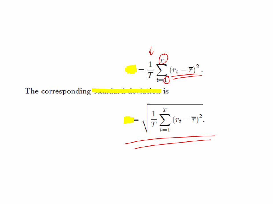
There is an alternative definition of the variance which is unbiased. This is now described.

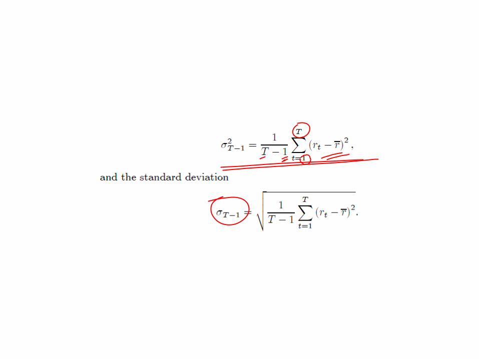
The unbiased estimator of the true variance is defined by

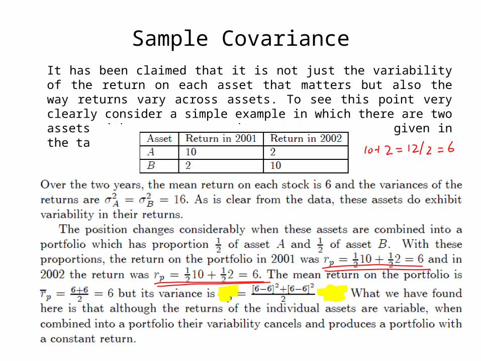
Sample CovarianceIt has been claimed that it is not just the variability of the return on each asset that matters but also the way returns vary across assets. To see this point very clearly consider a simple example in which there are two assets with returns over the past two years as given in the table below.

The feature of the example that gives rise to this result is that in a year in which the return on one asset is high, the return on the other asset is low. Put another way, as we move between years an increase in return on one of the assets is met with an equal reduction in the return on the other. This teaches a fundamental lesson for portfolio theory: it is not just the variability of asset returns that matters but how the returns on the assets move relative to each other. In our example the moves are always in opposite directions and this was exploited in the design of the portfolio to eliminate portfolio variability.

In the same way that the variance is used to measure the variability of return of an asset or portfolio, we can also provide a measure of the manner in which the returns on different assets move relative to each other. To do this we need to define the covariance between the returns on two assets, which is the commonly-used measure of whether the returns move together or in opposite directions.

Expectations

The first step in developing this new perspective is to consider the formation of expectations. Although not essential for using the formulas developed below, it is important for understanding their conceptual basis.

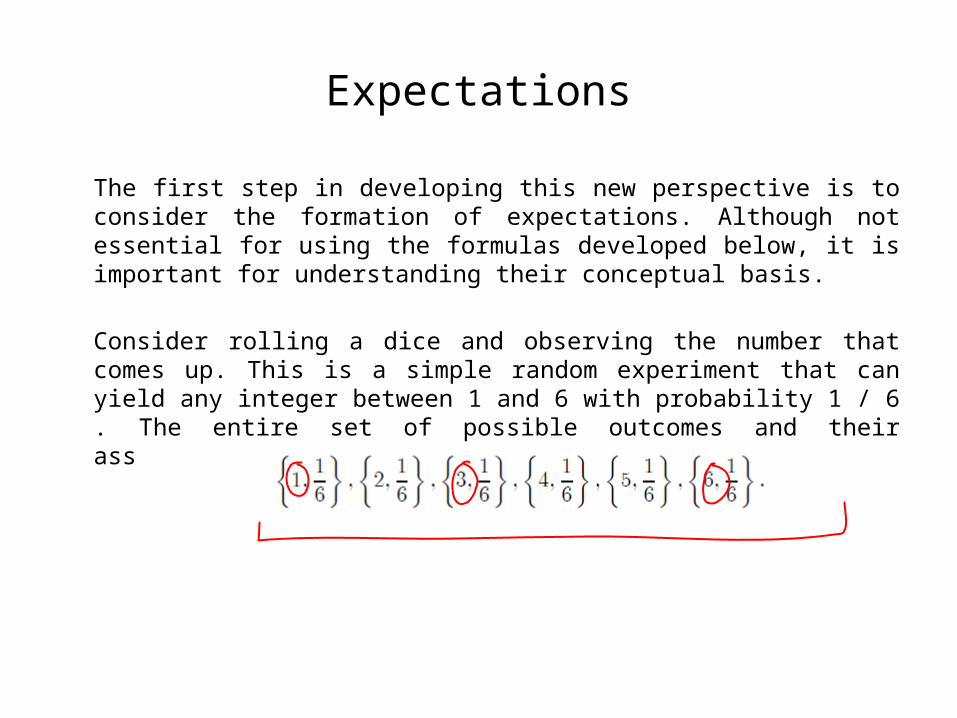
Consider rolling a dice and observing the number that comes up. This is a simple random experiment that can yield any integer between 1 and 6 with probability 1 / 6 . The entire set of possible outcomes and their associated probabilities is then

Expectations

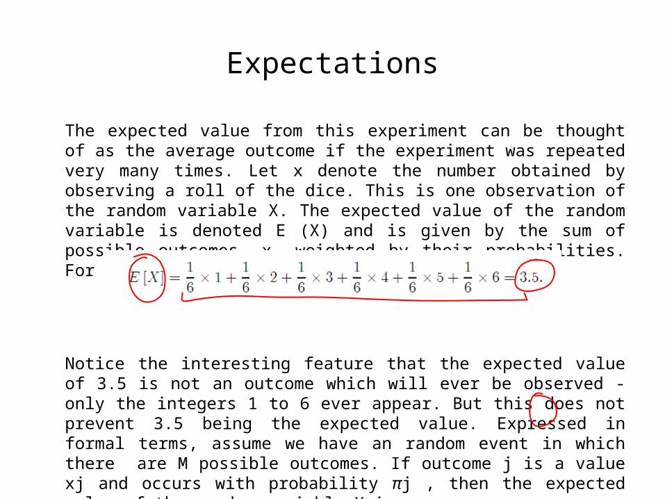
The expected value from this experiment can be thought of as the average outcome if the experiment was repeated very many times. Let x denote the number obtained by observing a roll of the dice. This is one observation of the random variable X. The expected value of the random variable is denoted E (X) and is given by the sum of possible outcomes, x, weighted by their probabilities. For the dice experiment the expected value is

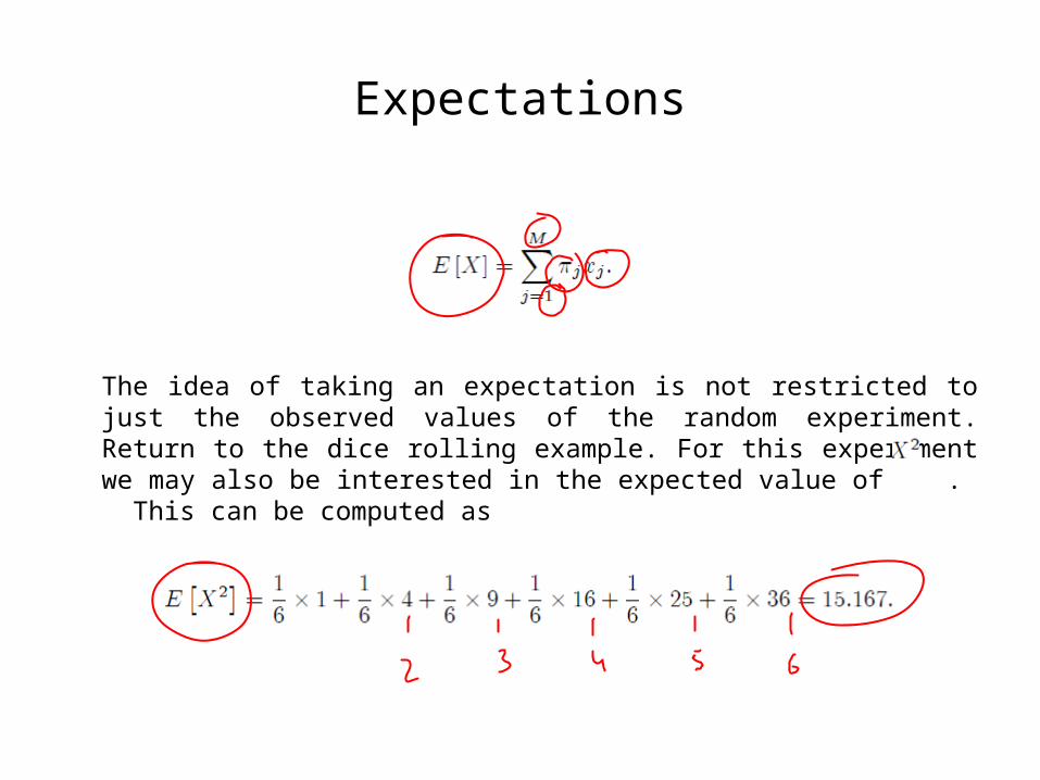
Notice the interesting feature that the expected value of 3.5 is not an outcome which will ever be observed - only the integers 1 to 6 ever appear. But this does not prevent 3.5 being the expected value. Expressed in formal terms, assume we have an random event in which there are M possible outcomes. If outcome j is a value xj and occurs with probability πj , then the expected value of the random variable X is

Expectations

The idea of taking an expectation is not restricted to just the observed values of the random experiment. Return to the dice rolling example. For this experiment we may also be interested in the expected value of . This can be computed as

Thank you