Page 1 of 10

Investing in Volatility

Published in Futures and Options World 1998Special Supplement on the 25th Annivesary of the Publication of the Black-Scholes Model

Emanuel DermanMichael Kamal

Iraj KaniJohn McClureCyrus PirastehJoseph Z. Zou

Page 2 of 10

Table of Contents

INTRODUCTION........................................................................................................3

A Brief History of Interest Rates...............................................................3

The Past and Future of Index Volatility1 ..................................................3

WHAT WE MEAN WHEN WE TALK ABOUT VOLATILITY .......................................4

INVESTING IN INDEX VOLATILITY ...........................................................................5

Trading Implied Volatility with Options ...................................................5

Isolating Local Volatility with Gadgets.....................................................5

Trading Real;zed Volatility by Hedging Options......................................6

USING REALIZED VOLATILITY CONTRACTS............................................................7

THE ADVANTGE OF VOLATILITY CONTRACTS........................................................7

THE SYNTHETIC CAPTURE OF REALIZED VOLATILITY ...........................................8

Page 3 of 10

mea-

today.ve.

h mir-are just

ard rate

ent

ccessfule for-

luationest rate the yielding.

role ofrs thatde the

INTRODUCTION

A Brief History of Interest Rates

In the beginning was the bond1, its value measured simply by its price. Soon, analysts invented better sures of relative bond value: current yield, which led to yield to maturity, followed by the term structure ofyields, the zero coupon yield curve, and finally forward rates and the forward rate curve. Their importancereflected the fact that these future rates can be locked in, once and for all, using bond portfoliosFrom then on, every interest rate trader and analyst carried in his head an abstract forward rate cur

Thinking in terms of forward rates stimulated the development of new derivative instruments whicrored the underlying reality of forward rates; Eurodollar futures contracts and interest rate swaps two examples. But as far as the valuation and analysis of these instruments was concerned, the forwcurve was a deterministic, static parameter whose future evolution had no impact on the current instrumvalue.

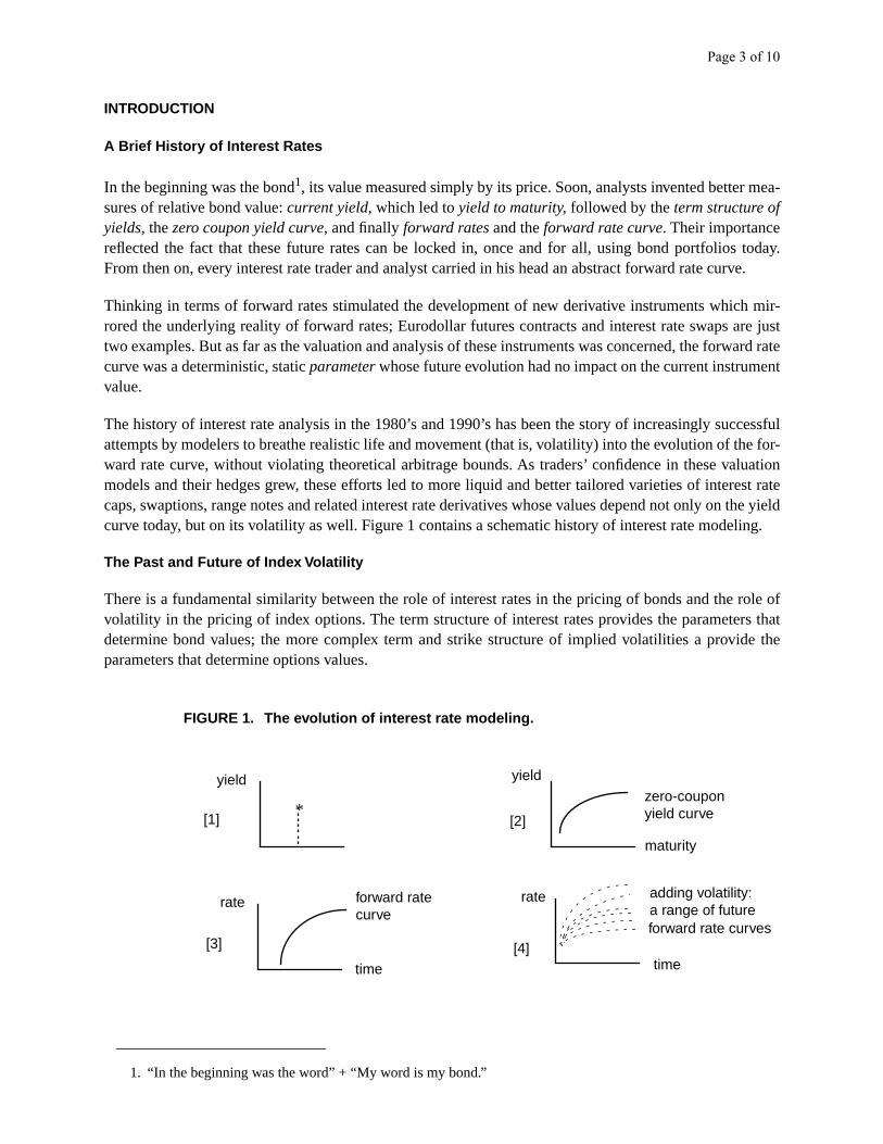
The history of interest rate analysis in the 1980’s and 1990’s has been the story of increasingly suattempts by modelers to breathe realistic life and movement (that is, volatility) into the evolution of thward rate curve, without violating theoretical arbitrage bounds. As traders’ confidence in these vamodels and their hedges grew, these efforts led to more liquid and better tailored varieties of intercaps, swaptions, range notes and related interest rate derivatives whose values depend not only oncurve today, but on its volatility as well. Figure 1 contains a schematic history of interest rate model

The Past and Future of Index Volatility

There is a fundamental similarity between the role of interest rates in the pricing of bonds and thevolatility in the pricing of index options. The term structure of interest rates provides the parametedetermine bond values; the more complex term and strike structure of implied volatilities a proviparameters that determine options values.

1. “In the beginning was the word” + “My word is my bond.”

FIGURE 1. The evolution of interest rate modeling.

*

yield yield

maturity

zero-couponyield curve

rate

time

forward ratecurve

time

rate

[1] [2]

[3] [4]

adding volatility:

forward rate curvesa range of future

Page 4 of 10

h bondarket

bond

fo-

tself,of vol-s, and

of vol-

n, for

daily

Volatility first entered the options world as a single parameter in the Black-Scholes formula. As eacwas characterized by its own yield to maturity, so each option had its own implied volatility. Soon, mparticipants began to abstract a term and strike structure of implied volatility – an implied volatility surfacefor each option strike and expiration – that was the two-dimensional analog of the yield curve for bonds. Asmarket yield curves imply a curve of attainable forward rates which can be theoretically locked in viaportfolios, so market implied volatilities uniquely determine a surface of attainable future local volatilities,

varying with market level and future time1, which can be theoretically locked in by index options portlios.

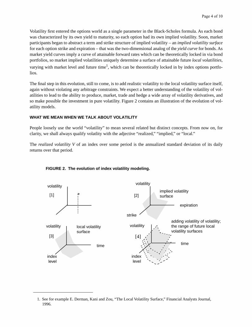
The final step in this evolution, still to come, is to add realistic volatility to the local volatility surface iagain without violating any arbitrage constraints. We expect a better understanding of the volatility atilities to lead to the ability to produce, market, trade and hedge a wide array of volatility derivativeso make possible the investment in pure volatility. Figure 2 contains an illustration of the evolution atility models.

WHAT WE MEAN WHEN WE TALK ABOUT VOLATILITY

People loosely use the world “volatility” to mean several related but distinct concepts. From now oclarity, we shall always qualify volatlity with the adjective “realized,” “implied,” or “local.”

The realized volatility V of an index over some period is the annualized standard deviation of its returns over that period.

1. See for example E. Derman, Kani and Zou, “The Local Volatility Surface,” Financial Analysts Journal, 1996.

FIGURE 2. The evolution of index volatility modeling.

*[1] [2]

[3] [4]

volatilityvolatility

expiration

strike

implied volatilitysurface

volatility

time

index level

index level

time

volatilityadding volatility of volatility;the range of future localvolatility surfaces

local volatilitysurface

Page 5 of 10

tyleholes

tilities

g

are the

gh the

urity; es

riceck inlow.

o gainquityt thel risk,

y-

po-

future-coupon is zero.osurerd rate

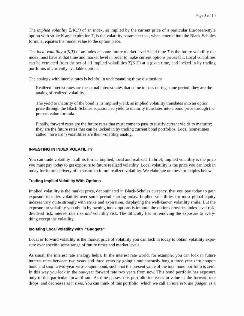
The implied volatility Σ(K,T) of an index, as implied by the current price of a particular European-soption with strike K and expiration T, is the volatility parameter that, when entered into the Black-Scformula, equates the model value to the option price.

The local volatility σ(S,T) of an index at some future market level S and time T is the future volatility theindex must have at that time and market level in order to make current options prices fair. Local volacan be extracted from the set of all implied volatilities Σ(K,T) at a given time, and locked in by tradinportfolios of currently available options.

The analogy with interest rates is helpful in understanding these distinctions.

Realized interest rates are the actual interest rates that come to pass during some period; theyanalog of realized volatility.

The yield to maturity of the bond is its implied yield; as implied volatility translates into an optionprice through the Black-Scholes equation, so yield to maturity translates into a bond price throupresent value formula.

Finally, forward rates are the future rates that must come to pass to justify current yields to matthey are the future rates that can be locked in by trading current bond portfolios. Local (sometimcalled “forward”) volatilities are their volatility analog.

INVESTING IN INDEX VOLATILITY

You can trade volatility in all its forms: implied, local and realized. In brief, implied volatility is the pyou must pay today to get exposure to future realized volatility. Local volatility is the price you can lotoday for future delivery of exposure to future realized volatility. We elaborate on these principles be

Trading Implied Volatility With Options

Implied volatility is the market price, denominated in Black-Scholes currency, that you pay today texposure to index volatility over some period starting today. Implied volatilities for most global eindexes vary quite strongly with strike and expiration, displaying the well-known volatility smile. Buexposure to volatility you obtain by owning index options is impure: the options provides index levedividend risk, interest rate risk and volatility risk. The difficulty lies in removing the exposure to everthing except the volatility.

Isolating Local Volatility with “Gadgets”

Local or forward volatility is the market price of volatility you can lock in today to obtain volatility exsure over specific some range of future times and market levels.

As usual, the interest rate analogy helps. In the interest rate world, for example, you can lock ininterest rates between two years and three years by going simultaneously long a three-year zerobond and short a two-year zero-coupon bond, such that the present value of the total bond portfolioIn this way you lock in the one-year forward rate two years from now. This bond portfolio has exponly to this particular forward rate. As time passes, this portfolio increases in value as the forwadrops, and decreases as it rises. You can think of this portfolio, which we call an interest-rate gadget, as a

Page 6 of 10

tes. Fig-

e

a

outas zero

weeny buy-

we can

ndex hedg-ility, as

t, -

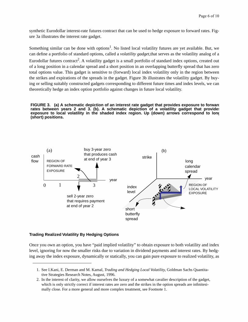
synthetic Eurodollar interest-rate futures contract that can be used to hedge exposure to forward raure 3a illustrates the interest rate gadget.

Something similar can be done with options1. No listed local volatility futures are yet available. But, wcan define a portfolio of standard options, called a volatility gadget,that serves as the volatility analog of

Eurodollar futures contract2. A volatility gadget is a small portfolio of standard index options, createdof a long position in a calendar spread and a short position in an overlapping butterfly spread that htotal options value. This gadget is sensitive to (forward) local index volatility only in the region betthe strikes and expirations of the spreads in the gadget. Figure 3b illustrates the volatility gadget. Bing or selling suitably constructed gadgets corresponding to different future times and index levels, theoretically hedge an index option portfolio against changes in future local volatility.

Trading Realized Volatility By Hedging Options

Once you own an option, you have “paid implied volatility” to obtain exposure to both volatility and ilevel, ignoring for now the smaller risks due to variation in dividend payments and interest rates. Bying away the index exposure, dynamically or statically, you can gain pure exposure to realized volat

1. See I.Kani, E. Derman and M. Kamal, Trading and Hedging Local Volatility, Goldman Sachs Quantita-tive Strategies Research Notes, August, 1996.

2. In the interest of clarity, we allow ourselves the luxury of a somewhat cavalier description of the gadgewhich is only strictly correct if interest rates are zero and the strikes in the option spreads are infinitesimally close. For a more general and more complex treatment, see Footnote 1.

FIGURE 3. (a) A schematic depiction of an interest rate gadget that provides exposure to forwar drates between years 2 and 3. (b). A schematic depiction of a volatility gadget that provide sexposure to local volatility in the shaded index region. Up (down) arrows correspond to lon g(short) positions.

0

2

3

(a)

1

sell 2-year zerothat requires paymentat end of year 2

buy 3-year zerothat produces cashat end of year 3

year

REGION OF

FORWARD RATE

EXPOSURE

(b)cashflow

strike

index level

year

calendarspread

long

shortbutterflyspread

REGION OFLOCAL VOLATILITYEXPOSURE

Page 7 of 10

nd have tohere liquid-s wellbuying a.

latili-atelyer-all riskyotective

e point

ur-y ulti-

ill beat is

olio’s

o buyd: theyoses its

r-

e

we shall demonstrate towards the end of this article in the section entitled “The Synthetic Capture ofRealized Volatility” on page 8. But capturing pure volatility is difficult: perfect hedging is impossible afrequent rehedging is expensive, especially close to expiration. Also, as the market moves you mayroll into new options to maintain a constant volatility sensitivity. Capturing volatility is also risky: tmay be unhedgeable index jumps, variation in volatility both foreseen and unforeseen, and varyingity. In short, sophisticated investors in pure volatility need complex analytical skills and software, aas good market instincts, in order to carry out these strategies. For this reason, clients may prefer contractfrom a dealer that delivers pure realized volatility, leaving to them the mechanics of capture

Capturing realized volatility involves trading options whose price is determined by their implied voties. Therefore, the fair value of a derivative contract that delivers pure realized volatility is approximequal to the level of current implied volatility. Historically, implied index volatility is typically several pcentage points higher than past realized volatility over the same period, probably because, as with products, market makers determine prices by factoring in their transactions costs as well some prrisk premium.

USING REALIZED VOLATILITY CONTRACTS

As pointed out, the fair purchase level for realized volatility V is, roughly speaking, the current

implied volatility1 Σ. A realized volatility contract is a forward contract on realized volatility V whose delivery price is Σ. The purchaser of the contract with a face value of $1 receives (pays) $1 for every percentagby which realized volatility V over the life of the contract exceeds (is exceeded by) Σ.

The purchaser of a realized volatility contract will benefit if future realized volatility is greater than crent implied levels. He is seeking to gain from a belief in future uncertainty, even if that uncertaintmately leads to no permanent long-term change in index level.

The seller of a realized volatility contract seeks to gain from a belief that future realized volatility wappreciably lower than current implied volatility. The owner of a broad portfolio of index options thlong volatility at a variety of market strikes may find this a simpl one-stop way to liquidate the portfvolatility exposure after a runup in implied volatility levels.

THE ADVANTAGE OF VOLATILITY CONTRACTS

Realized volatility contracts aren’t the only way to invest in pure volatility. For example, you can alsvolatility using at-the-money straddles, whose value increases with volatility. But straddles are hybriprovide both market and volatility exposure. As the market moves away from the strike, a straddle l

1. Volatility mavens will realize that the implied volatilities of individual S&P options vary strongly with strike, expiration and market level. In practice a more careful view of implied volatility as the cost of puchasing realized volatility may be necessary, taking into account the important effects of the volatility skew and term structure. In the interest of clarity, we ignore most of these subtleties here, though thesdetails obviously effect the engineering and pricing of volatility contracts.

Page 8 of 10

n andrtain

relatedn foreignacts

expira-d vol-

f

nd

n a ran-nitude

nal toare of

-

ge

ies.The moves.

relatively pure sensitivity to volatility, and evolves into a more complex bet on both market directiovolatility. In order to regain its pure volatility sensitivity, the straddle will have to be rolled at uncefuture market levels and trading costs.

In contrast, realized volatility contracts provide pure volatility exposure by design. They provide astraightforward means for clients to accumulate or dispose of volatility as a primary asset, with no index exposure at all. In the same way as guaranteed exchange rate (Quantos) futures contracts ostock indexex allow allow investment in foreign markets without exchange-rate risk, so volatility contrallow index volatility acquisition without index risk.

In principle, volatility contracts can be liquidated at some intermediate date between inception and tion. As with any forward contract, the value on that date will depend upon both the prevailing implieatility structure and the volatility realized thus far.

THE SYNTHETIC CAPTURE OF REALIZED VOLATILITY

In this section we explain how to synthesize pure realized volatility exposure.

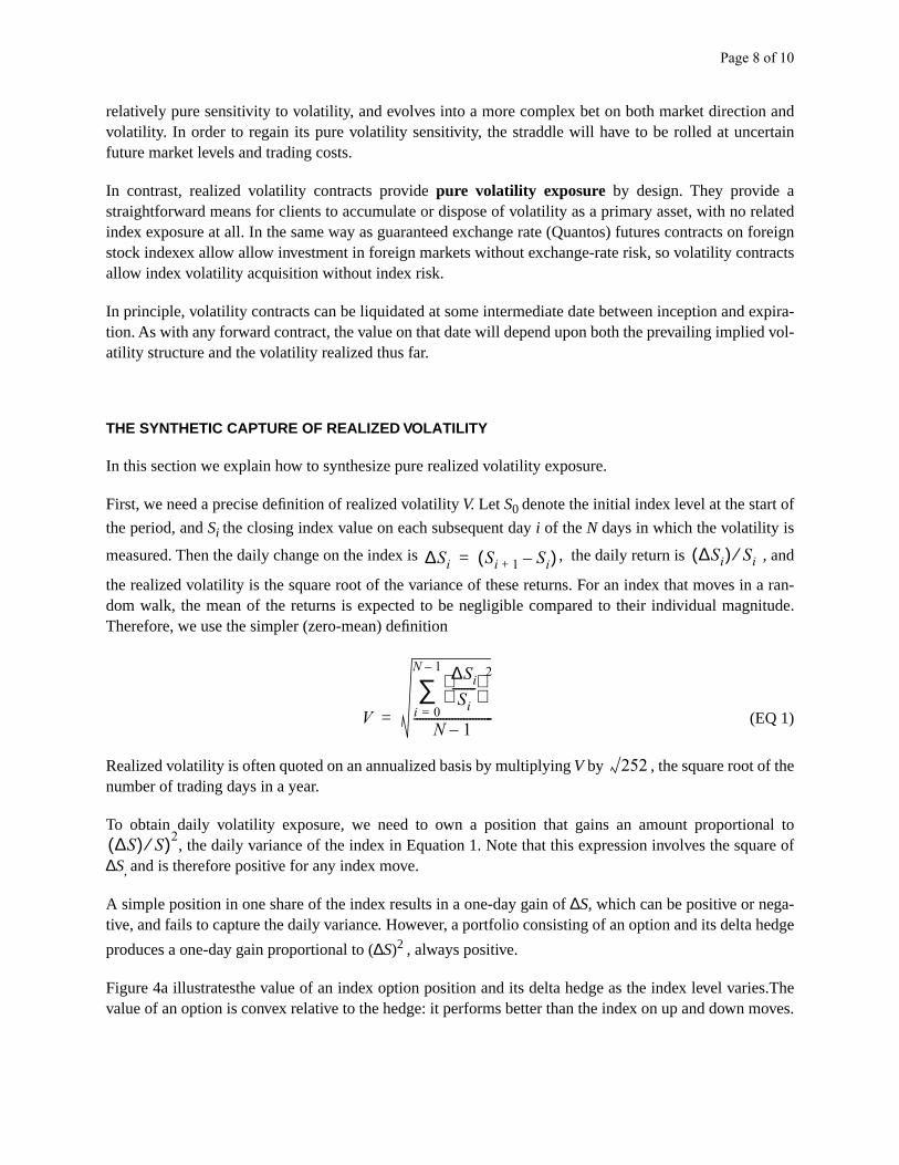
First, we need a precise definition of realized volatility V. Let S0 denote the initial index level at the start o

the period, and Si the closing index value on each subsequent day i of the N days in which the volatility is

measured. Then the daily change on the index is , the daily return is , a

the realized volatility is the square root of the variance of these returns. For an index that moves idom walk, the mean of the returns is expected to be negligible compared to their individual mag.Therefore, we use the simpler (zero-mean) definition

(EQ 1)

Realized volatility is often quoted on an annualized basis by multiplying V by , the square root of thenumber of trading days in a year.

To obtain daily volatility exposure, we need to own a position that gains an amount proportio, the daily variance of the index in Equation 1. Note that this expression involves the squ

∆S, and is therefore positive for any index move.

A simple position in one share of the index results in a one-day gain of ∆S, which can be positive or negative, and fails to capture the daily variance. However, a portfolio consisting of an option and its delta hed

produces a one-day gain proportional to (∆S)2 , always positive.

Figure 4a illustratesthe value of an index option position and its delta hedge as the index level varvalue of an option is convex relative to the hedge: it performs better than the index on up and down

∆Si Si 1+ Si–( )= ∆Si( ) Si⁄

V

∆Si

Si--------

2

i 0=

N 1–

∑N 1–

---------------------------=

252

∆S( ) S⁄ )2

Page 9 of 10

all shift

oves upre

and of

eves, and

tionsmoves

in

g some

breaks

own-

f

e-

whose

s that

-

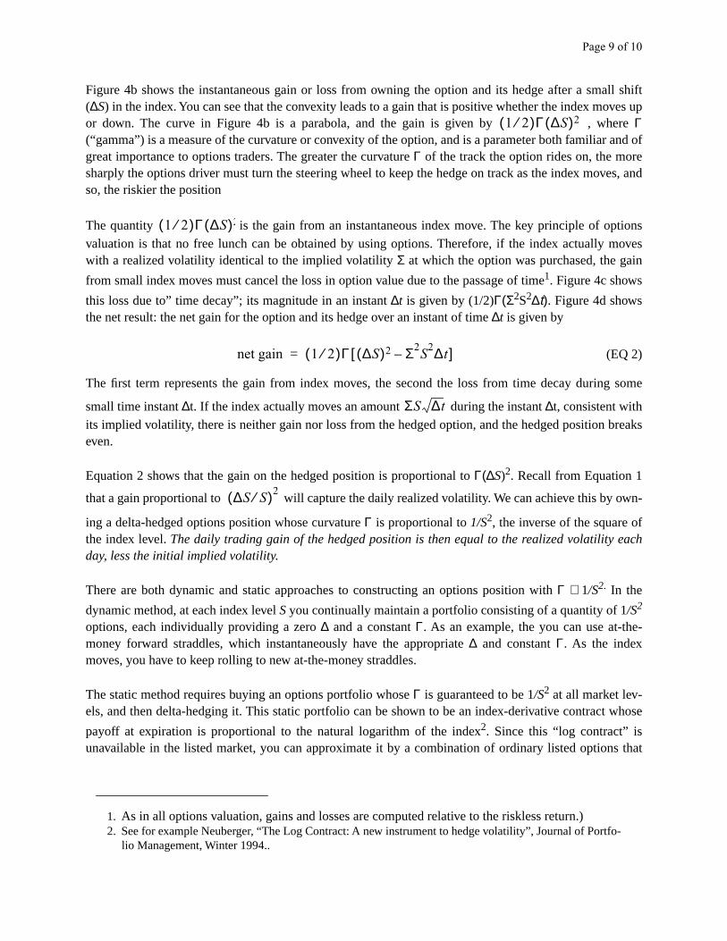
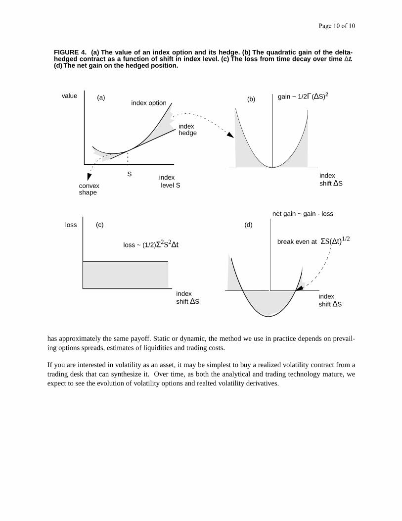
Figure 4b shows the instantaneous gain or loss from owning the option and its hedge after a sm(∆S) in the index. You can see that the convexity leads to a gain that is positive whether the index mor down. The curve in Figure 4b is a parabola, and the gain is given by , wheΓ(“gamma”) is a measure of the curvature or convexity of the option, and is a parameter both familiargreat importance to options traders. The greater the curvature Γ of the track the option rides on, the morsharply the options driver must turn the steering wheel to keep the hedge on track as the index moso, the riskier the position

The quantity is the gain from an instantaneous index move. The key principle of opvaluation is that no free lunch can be obtained by using options. Therefore, if the index actually with a realized volatility identical to the implied volatility Σ at which the option was purchased, the ga

from small index moves must cancel the loss in option value due to the passage of time1. Figure 4c shows

this loss due to” time decay”; its magnitude in an instant ∆t is given by (1/2)Γ(Σ2S2∆t). Figure 4d showsthe net result: the net gain for the option and its hedge over an instant of time ∆t is given by

(EQ 2)

The first term represents the gain from index moves, the second the loss from time decay durin

small time instant ∆t. If the index actually moves an amount during the instant ∆t, consistent withits implied volatility, there is neither gain nor loss from the hedged option, and the hedged position even.

Equation 2 shows that the gain on the hedged position is proportional to Γ(∆S)2. Recall from Equation 1

that a gain proportional to will capture the daily realized volatility. We can achieve this by

ing a delta-hedged options position whose curvature Γ is proportional to 1/S2, the inverse of the square othe index level. The daily trading gain of the hedged position is then equal to the realized volatility eachday, less the initial implied volatility.

There are both dynamic and static approaches to constructing an options position with Γ ∼ 1/S2. In the

dynamic method, at each index level S you continually maintain a portfolio consisting of a quantity of 1/S2

options, each individually providing a zero ∆ and a constant Γ. As an example, the you can use at-thmoney forward straddles, which instantaneously have the appropriate ∆ and constant Γ. As the indexmoves, you have to keep rolling to new at-the-money straddles.

The static method requires buying an options portfolio whose Γ is guaranteed to be 1/S2 at all market lev-els, and then delta-hedging it. This static portfolio can be shown to be an index-derivative contract

payoff at expiration is proportional to the natural logarithm of the index2. Since this “log contract” isunavailable in the listed market, you can approximate it by a combination of ordinary listed option

1. As in all options valuation, gains and losses are computed relative to the riskless return.)2. See for example Neuberger, “The Log Contract: A new instrument to hedge volatility”, Journal of Portfo

lio Management, Winter 1994..

1 2⁄( )Γ ∆S( )2

1 2⁄( )Γ ∆S( )2

net gain 1 2⁄( )Γ ∆S( )2 Σ2S

2∆t–[ ]=

ΣS ∆t

∆S S⁄( )2

Page 10 of 10

prevail-

from aure, we

has approximately the same payoff. Static or dynamic, the method we use in practice depends oning options spreads, estimates of liquidities and trading costs.

If you are interested in volatility as an asset, it may be simplest to buy a realized volatility contract trading desk that can synthesize it. Over time, as both the analytical and trading technology matexpect to see the evolution of volatility options and realted volatility derivatives.

FIGURE 4. (a) The value of an index option and its hedge. (b) The quadratic gain of the delta-hedged contract as a function of shift in index level. (c) The loss from time decay over time ∆t.(d) The net gain on the hedged position.

index

value

index

S

level S

indexshift ∆S

gain ~ 1/2Γ(∆S)2index option

hedge

convexshape

loss

indexshift ∆S

(a) (b)

(c)

loss ~ (1/2)Σ2S2∆t

indexshift ∆S

(d)

net gain ~ gain - loss

break even at Σ S( ∆ t) 1/2