investigating high field gravity using astrophysical ... · compact stellar objects (white dwarf...
TRANSCRIPT
INVESTIGATING HIGH FIELD GRAVITY USING
ASTROPHYSICAL TECHNIQUES
Elliott D. Bloom
Stanford Linear Accelerator Center
Stanford University, Stanford, CA 94309
E. D. Bloom 1994

2
3
Table of Contents
Preface
1. Introduction
2. The Physics of Compact Stellar Objects
a. Schwarzschild Geometry
b. The Equation of of State of Compact Stellar Objects
c. The End State of Stars
(i) White Dwarfs
(ii) Neutron Stars
(iii) Strange Stars, Q-Stars, and Black Holes
(iv) Summary
3. Laboratories for Particle Astrophysics: X-Ray Stellar Binary Systems and Active Galactic
Nuclei (AGN)
a. Description of X-Ray Binary Systems
b. Description of Active Galactic Nuclei (AGN)
c. X-Ray Binary System Orbital Parameters
d. Using Orbital Parameters to Determine Compact Object Masses
(i) Some Leading Stellar Black Hole Candidates
(ii) The Black Hole Candidate in the AGN of M87
e. Using Fast X-Ray Timing to Measure the Compact Size of Compact Stellar
Objects
(i) X-Ray Timing Measurements for Cyg X-1
4. X-Ray Astrophysics
a. X-Ray Discriminants Black Holes vs. Neutron Stars
b. Future X-Ray Missions
(i) The Unconventional Stellar Aspect Experiment (USA)
(ii) The X-Ray Timing Explorer (XTE)
4
5. Gamma-Ray Astrophysics
a. Gamma-Ray Bursters
b. Results from High-Energy Gamma-Ray Experiments
(i) Space Based (mainly EGRET)
(ii) Ground Based
c. Future High-Energy Gamma-Ray Missions
6. Conclusions
7. Acknowledgments
8. Appendices
A. Introduction to Wavelet Methods
B. A List of Current Black Hole Candidates
9. References
5
Preface
The purpose of these lectures is to introduce particle physicists to astrophysical techniques.
These techniques can help us understand certain phenomena important to particle physics that
are currently impossible to address using standard particle physics experimental techniques. As
the subject matter is vast, compromises are necessary in order to convey the central ideas to the
reader. Many general references are included for those who want to learn more. The paragraphs
below elaborate on the structure of these lectures. I hope this discussion will clarify my
motivation and make the lectures easier to follow.
The lectures begin with a brief review of more theoretical ideas. First, elements of
general relativity are reviewed, concentrating on those aspects that are needed to understand
compact stellar objects (white dwarf stars, neutron stars, and black holes). I then review the
equations of state of these objects, concentrating on the simplest standard models from
astrophysics. After these mathematical preliminaries, Sec. 2(c) discusses The End State of Stars.
Most of this section also uses the simplest standard models. However, as these lectures are for
particle physicists, I also discuss some of the more recent approaches to the equation of state of
very dense compact objects. These particle-physics-motivated equations of state can dramatically
change how we view the formation of black holes.
Section 3 focuses on the properties of the objects that we want to characterize and
measure. X-ray binary systems and Active Galactic Nuclei (AGN) are stressed because the
lectures center on understanding very dense stellar objects, black hole candidates (BHCs), and
their accompanying high gravitational fields. The use of x-ray timing and gamma-ray
experiments is also introduced in this section.
Sections 4 and 5 review information from x-ray and gamma-ray experiments. These
sections also discuss the current state of the art in x-ray and gamma-ray satellite experiments and
plans for future experiments.
6
1. Introduction
Along with QCD and the electroweak forces, gravity is one of the fundamental forces of nature.
However, even though gravity was the earliest force to be described analytically and has more
recently been embodied in General Relativity (GR), a complete understanding of gravity has yet
to be found. The goal of a self-consistent quantum field theory of gravity still escapes us after
more than 60 years of effort. In addition, with our understanding of particle physics apparently
extended to the TeV mass range and our theoretical estimates of conditions in the early universe
reaching to the inflationary epoch at 10-30 sec and earlier, questions of the role of gravity in the
unification of the forces loom large.
My view is that physics is ultimately an experimental science, and so we need data, lots
of data, to make progress in our theoretical understanding. I suggest that the lack of progress in
understanding the deeper aspects of gravity comes from a dearth of even remotely related data.
How one might approach an experimental examination of strong field relativistic gravity and
related topics is one of the main subjects of these lectures. It is not easy to decide what to do, and
once decided, not easy to accomplish. The relevant experimental approaches are all very
difficult; however, we have to start somewhere.
2. The Physics of Compact Stellar Objects
One place we believe that the full power of GR is needed to describe the physics, and hence can
be tested, is in the immediate neighborhood of compact stellar objects. Such objects include
white dwarfs, neutron stars, and black holes. This section explores the character of these objects
and briefly develops current models that describe them.
2a. Schwarzschild Geometry
The physics of compact stellar objects requires two major components––gravity and an equation
of state. Gravity, which we briefly describe in this section, results from the mass distribution of
the compact object. This mass distribution generates a space-time geometry predicted by GR,
which in turn produces the gravitational field that controls the structure of the compact object.1
Indeed, in the case of a compact object of sufficient mass, this space-time geometry leads to a
new type of object, a black hole, that is stranger than fiction. Black holes are not just a new type
of stellar object. Their properties, as predicted by GR, challenge our basic understanding of
quantum mechanics, particle physics, and space-time itself.2
7
In GR, the only spherically symmetric gravitational field solution in vacuum is static.
This space-time geometry is named after Schwarzschild, who first derived it from the GR field
equations. The Schwarzschild space-time geometry is represented by the metric
dsM
rdt
drM
r
r d d2 22
2 2 2 212
12
= − − +−
+ +( ) ( sin )θ θ ϕ (1)
with the choice of units such that c (speed of light) = G(gravitational constant) = 1. In the weak
field limit, Schwarzschild space-time geometry becomes Newtonian gravity from a central mass,
M, in flat space-time.
In the case of compact stellar objects that are not black holes, M → mass within radius r,
or m(r), and the factor [1-2m(r)/r]-1 does not become singular at r = 2 M, because m(r) decreases
sufficiently fast with decreasing r; that is, the radius r = 2 M lies inside the matter distribution of
the compact object. (M in this case is the total mass of the star.) A black hole solution results
when this is not the case. For black holes, r = 2 M lies outside the matter distribution of the
compact object. In general, Rsch ≡ 2 GM/c2 = 2 M ≅ 3(M/M§) [km], where M§ is the sun’s mass
and defines the “Schwarzschild horizon” or “Schwarzschild radius,” or in current parlance, the
“event horizon.” In the case of black holes, r = 2 M seems a badly behaved region of the
Schwarzschild geometry, as the metric appears to diverge to infinity. However, the space-time
geometry is not singular there.
As described in Chapter 31 of Misner, Throne, and Wheeler (MTW)1, to determine
whether or not the space-time geometry is singular at the horizon radius of a black hole, send an
astronaut in from far away to chart it (as happened recently on the TV program “Star Trek
Voyager”). For simplicity, let the astronaut fall freely and radially toward the horizon. The radial
geodesic of the Schwarzschild metric in the astronaut’s rest frame gives, in terms of his/her
proper time, τ,
τ2
2
3 21
3
2
M
r
Mconst= − +( ) . (2)
While for an observer far away (Schwarzschild-coordinate time t) the time it takes for the
astronaut to fall is
8
t
M
r
M
r
M
rMr
M
const2
2
3 22
22
1
21
23
2
1
2
1
2
1
2
= − − ++
−+( ) ( ) ln
( )
( )
. (3)
Figure 1 shows the trajectories derived from Eqs. (2) and (3) (for a particular initial condition).
Of all the features of the astronaut’s trajectory, one stands out most clearly and disturbingly: to
reach the horizon, r = 2 M (the dotted line in the figure) requires a finite lapse of proper time, but
an infinite lapse of coordinate time. The traveler passes through the horizon to be inexorably
crushed by the black hole’s “true” singularity at r = 0 in a bit over τ = 16/M, while to the far
away observer, the astronaut just redshifts from sight,3 approaching the horizon as t → ∞.
Of course, proper time is the relevant quantity for the explorer’s heartbeat and health. No
coordinate system has the power to prevent the inevitable in fall to r = 0. Only the coordinate-
independent geometry of space-time could possibly do that, and Eq. (2) shows that it does not!
The Schwarzschild metric is well-suited to describe a spherically symmetric star with
zero angular momentum. The metric is used in the calculations of the properties of compact
stellar objects that approximate these conditions. Figure 2, from Chapter 23 of MTW,
schematically displays the geometry within (dark gray) and around (white) a spherically
symmetric star of radius R = 2.66 M. The star is in hydrostatic equilibrium and has zero angular
momentum. The two-dimensional geometry
[ ]ds m r r dr r d2 1 2 2 21 2= − +−( ) / ϕ (4)
of an equatorial slice through the star at fixed time (θ = π/2, t = t0) is represented as embedded in
Euclidean three-space in such a way that distances between any two nearby points in the surface
are shown correctly. Distances measured out of the curved surface have no physical meaning.
The embedding three-space itself also has no physical meaning and is just used as a tool to show
the curved two-geometry induced by the star’s mass.
Because of the relatively simple form of Eq. (1), the coordinates have a direct physical
interpretation. For the Schwarzschild geometry displayed in the figure, at any radius r there is a
two-dimensional spherical surface centered about the point r = 0, and θ, ϕ are conventional polar
9
coordinates on the two-sphere. The quantity r is defined by setting the proper circumference of
the two-sphere to 2 πr. This circumference in curved two-geometry corresponds to a sphere of
proper area 4 πr2 in the three-geometry of real Euclidean space (not the embedding three-space
of the figure). Note that due to the metric of curved space, the proper distance R, between r = 0
and the point labeled by r on a radial line in this space, is larger than r and 4 πR2 > 4 πr2. This
correspondence, r → 4 πr2, allows one to visualize the entire three-geometry in and around the
star at any time t.
2b. The Equation of State of Compact Stellar Objects
Besides the gravitational field, the physics of the compact stellar object must be put into the
(highly nonlinear) equations that predict the space-time structure of these objects and their
surroundings. Compact stellar objects evolve from stellar objects. A stellar object refers to a star
at any time during its evolution. In its nuclear burning phase, the stellar object is usually a main
sequence star, such as our sun. Depending on its mass and history, at the end of its evolution, the
stellar object can collapse to a compact stellar object. Stars “die” when most of their nuclear fuel
has been consumed.4 White dwarfs, neutron stars, and black holes are “born” when normal stars
“die.”
The equation of state of a stellar object gives the relationship between its pressure and
density,
P = P(ρ). (5)
This equation incorporates the underlying microphysics as local thermodynamic relationships of
an individual matter element. However, the microphysics is the determining factor. Thus, our
understanding of the basic physics at the extreme conditions existing in compact objects is
central to the success of the theory. In the case of black hole formation, the correct microphysics
could possibly require input from particle physics beyond the Standard Model, while current
theories typically include only idealistic approximations from nuclear physics and lower energy
scales.
In kinetic theory, the number density in phase space for each species of particle,
dn
d xd p3 3
, provides a complete description of the system.5 The main thermodynamic variables
10
we will be considering are density and pressure. The density is formally given as the total energy
per unit volume, where the total energy of a particle species, j, with three-momentum magnitude
pj and mass mj, is (with c = 1)
E p mj j j= +2 2 . (6)
The energy density is then
ε = ∫ Edn
d xd pd p
3 33
. (7)
The pressure, P, is the “flow of momentum density” and is given for an isotropic medium by
P n p r v r pvdn
d xd pd p
p
E
dn
d xd pd p= ⋅ ⋅ =
=
∫ ∫( $)( $)
r r 1
3
1
33 33
2
3 33 , (8)
where
ndn
d xd pd p=
∫ 3 3
3 (9)
is the number density of each species of particles, rp is the three momentum,
rv is the three
velocity, and $r is a unit vector defining a direction. The factor of 1/3 comes from assumed
isotropy. Note that for massless particles, P = ε/3.
Using the number density, we can define an equivalent dimensionless distribution
function in phase space, F, that gives the Lorentz invariant average occupation number of a cell
in phase space. As d3xd3p is a scalar under a Lorentz transformation, F is also.
dn
d xd p
g
hF x p t
3 3 3
= ( , , ),
r r (10)
11
where h is Planck’s constant, h3 is the volume of a cell in phase space, and g is the statistical
weight for a particle species. Here, g = 2 S+1 for massive particles with spin S. For photons, g =
2, and for neutrinos, g = 1 (as there are only left-handed neutrinos).
For an ideal gas in equilibrium, F has the simple form
[ ]F Ee E kT
( )( )/
=±−
1
1µ(11)
where the “+” sign corresponds to fermions (Fermi-Dirac statistics), and the “−” sign to bosons
(Bose-Einstein statistics). In Eq. (11), T is the temperature, k is Boltzmann’s constant, and µ is
the chemical potential for the species.
For sufficiently low particle densities and high T, F(E) becomes the Maxwell-Boltzmann
distribution
F E eE
kT( ) ≈−
µ
<< 1. (12)
For completely degenerate fermions (T → 0, i.e., µ/kT → ∞), µ is identified with the Fermi
Energy, EF, and,
F EE E
E EF
F
( ),
,=
≤>
1
0. (13)
As an example, we derive the equation of state of a completely degenerate, single species, ideal
(noninteracting) Fermi gas.6 This very idealized equation of state actually has approximate
validity in describing isolated white dwarf and neutron stars. These compact stellar objects
ultimately cool to zero temperature. At T ≅ 0, it is the degeneracy pressure of electrons in the
case of white dwarfs, and neutrons in the case of neutron stars, that support these stars against
gravitational collapse. More realistic, and consequently more complex, equations of state
describing white dwarfs and neutron stars can be found in the literature.7
Let us start with the electron gas case that applies to white dwarfs. The gas can be treated
as ideal if all electromagnetic interactions are neglected. We concentrate on the degeneracy
12
force, which is the dominant force between the electrons at very high density. We define the
Fermi momentum, pF, by
E p mF F e= +2 2 . (14)
Equations (9), (10), and (13) then give
nh
p dph
pe
p
F
F
= =∫2
48
332
0 33π
π. (15)
We define a dimensionless Fermi momentum
xF = pF/me . (16)
Then Eq. (15) becomes
nx
eF
e
=3
2 33π D, (17)
where
D he em c= = × −/ .3 862 10 13 m (18)
is the electron Compton wavelength in SI units.
The degeneracy pressure from the electron gas is given by Eqs. (8), (10), (13), and (16),
Ph
p
p mp dp
m x dx
x
mxe
e
e eF
xp FF
=+
=+
=∫∫2
34
3 13
2
2 2
22 3
4
2 300π
πϕ
D D( ), (19)
where
13
ϕπ
( ) { ( )x x xx
F F FF= + − +
1
81
2
31
22
2
arcsinh(xF)}, (20)
and mec2/λe
3 = 1.422 x 1024 Pa (in SI units, 1 Pa = 1 Pascal = 1 Newton/m2).
Similarly, the energy density of the electron gas is given by Eqs. (7), (10), (13), and (16),
ε π χe ee
F
p
hp m p dp
mx
F= + =∫243
2 2 230 D
( ), (21)
where
χπ
( ) { ( )x x x xF F F F= + + −1
81 2 1
22 2 arcsinh(xF)}, (22)
and in this case, we take mec/λe3 = 1.422 x 1024 J/m3 .
When considering the equation of state of white dwarf stars, we see that the degenerate
electron gas contributes most of the pressure; however, the density is dominated by the rest-mass
of the ions. This baryon density, ρB, is given in terms of the weighted sum over masses of the
ion species i, mi ,
ρ B i ii
n m= ∑ , (23)
where ni is the number of ion types i per m3. The mean baryon rest mass, mB, is commonly used
in the literature, where
mn m
n A nB
i ii
i ii
B
B
≡ =∑∑
ρ , (24)
and Ai is the baryon number of the ith ionic species, while nB is the number of baryons per m3. All
of the quantities discussed above are usually considered in the center-of-mass frame of the star.
14
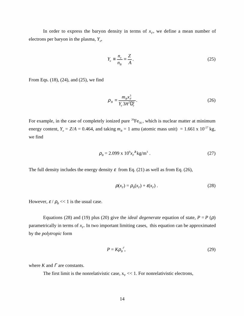
In order to express the baryon density in terms of xF, we define a mean number of
electrons per baryon in the plasma, Ye,
Yn
n
Z
Aee
B
≡ = . (25)
From Eqs. (18), (24), and (25), we find
ρπBB F
e e
m x
Y=
3
2 33 D. (26)
For example, in the case of completely ionized pure 26Fe56 , which is nuclear matter at minimum
energy content, Ye = Z/A = 0.464, and taking mB = 1 amu (atomic mass unit) = 1.661 x 10⁻²⁷ kg,
we find
ρB = 2.099 x 10⁹xF3 kg/m3 . (27)
The full density includes the energy density ε from Eq. (21) as well as from Eq. (26),
ρ(xF) = ρB(xF) + ε(xF) . (28)
However, ε / ρB << 1 is the usual case.
Equations (28) and (19) plus (20) give the ideal degenerate equation of state, P = P (ρ)
parametrically in terms of xF. In two important limiting cases, this equation can be approximated
by the polytropic form
P = KρBΓ, (29)
where K and Γ are constants.
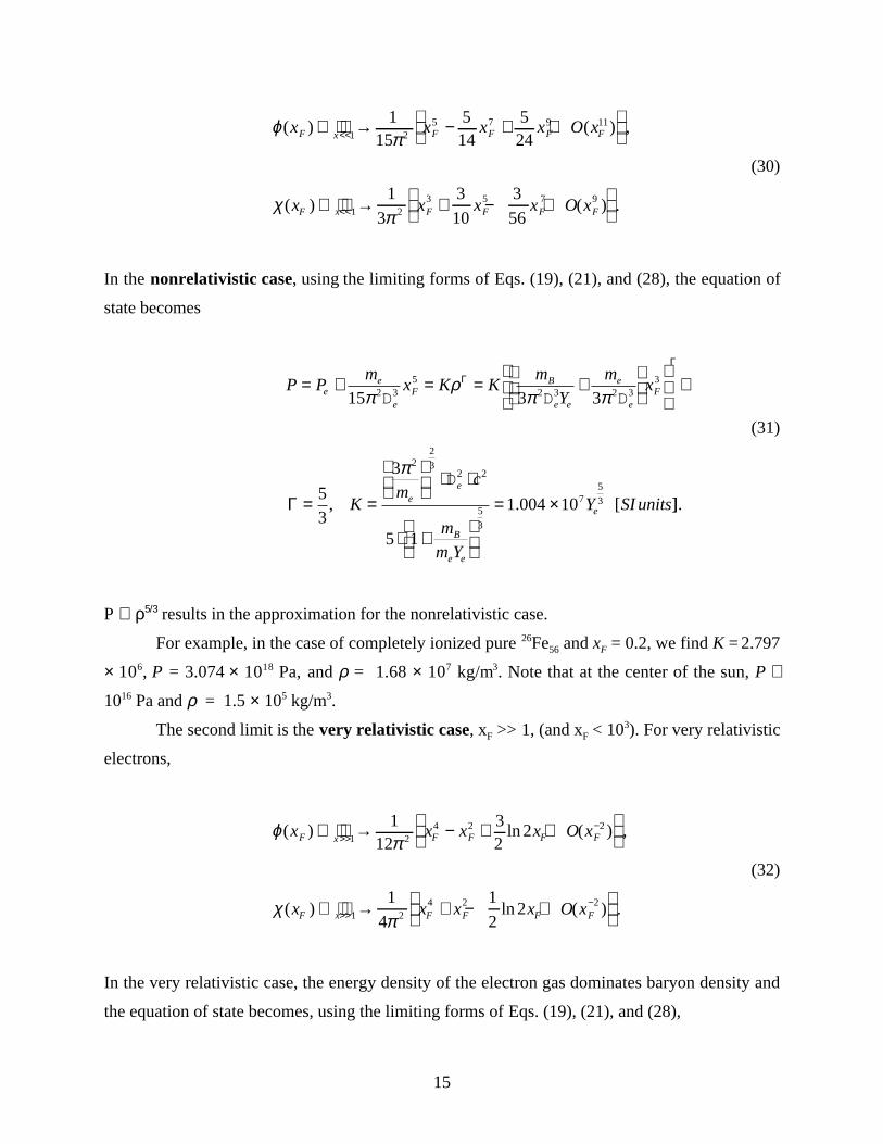
The first limit is the nonrelativistic case, xF << 1. For nonrelativistic electrons,
15
ϕπ
χπ
( ) ( ) ,
( ) ( ) .
x x x x O x
x x x x O x
F x F F F F
F x F F F F
<<
<<
→ − + +
→ + − +
1 25 7 9 11
1 23 5 7 9
115
514
524
1
3
3
10
3
56
(30)
In the nonrelativistic case, using the limiting forms of Eqs. (19), (21), and (28), the equation of
state becomes
P Pm
x K Km
Y
mx
Km
c
m
m Y
Y SI units
ee
eF
B
e e
e
eF
ee
B
e e
e
= ≅ = = +
⇒
= =
⋅ ⋅
⋅ +
= ×
15 3 3
53
3
5 1
1 004 10
2 35
2 3 2 33
22
32 2
5
3
75
3
πρ
π π
π
D D D
D
Γ
Γ
Γ , . [ ]].
(31)
P ∝ ρ5/3 results in the approximation for the nonrelativistic case.
For example, in the case of completely ionized pure 26Fe56 and xF = 0.2, we find K = 2.797
× 106, P = 3.074 × 10¹⁸ Pa, and ρ = 1.68 × 10⁷ kg/m3. Note that at the center of the sun, P ≅
1016 Pa and ρ = 1.5 × 10⁵ kg/m3.
The second limit is the very relativistic case, xF >> 1, (and xF < 103). For very relativistic
electrons,
ϕπ
χπ
( ) ln ( ) ,
( ) ln ( ) .
x x x x O x
x x x x O x
F x F F F F
F x F F F F
>>−
>>−
→ − + +
→ + − +
1 24 2 2
1 24 2 2
112
32
2
1
4
1
22
(32)
In the very relativistic case, the energy density of the electron gas dominates baryon density and
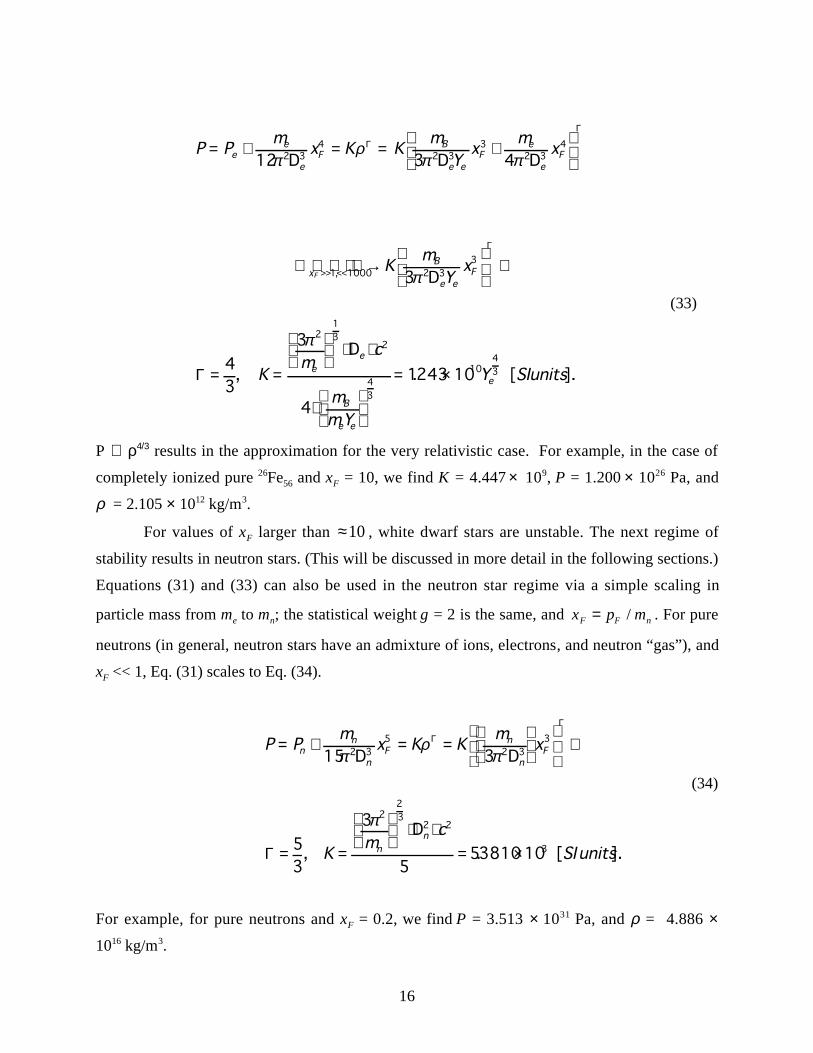
the equation of state becomes, using the limiting forms of Eqs. (19), (21), and (28),
16
P Pm
x K Km
Yx
mxe
e
eF
B
e eF
e
eF= ≅ = = +
12 3 42 3
42 3
32 3
4
πρ
π πD D DΓ
Γ
xB
e eF
ee
B
e e
e
FK
mY
x
Km
c
mmY
Y SIunits
>> << →
⇒
= =
⋅ ⋅
⋅
= ×
1 1000 2 33
213
2
43
1043
3
43
3
4
1243 10
,
, . [ ].
π
π
D
D
Γ
Γ
(33)
P ∝ ρ4/3 results in the approximation for the very relativistic case. For example, in the case of
completely ionized pure 26Fe56 and xF = 10, we find K = 4.447 × 10⁹, P = 1.200 × 1026 Pa, and
ρ = 2.105 × 10¹² kg/m3.
For values of xF larger than ≈10 , white dwarf stars are unstable. The next regime of
stability results in neutron stars. (This will be discussed in more detail in the following sections.)
Equations (31) and (33) can also be used in the neutron star regime via a simple scaling in
particle mass from me to mn; the statistical weight g = 2 is the same, and x p mF F n= / . For pure
neutrons (in general, neutron stars have an admixture of ions, electrons, and neutron “gas”), and
xF << 1, Eq. (31) scales to Eq. (34).
P Pm
x K Km
x
Km
cSIunits
nn
nF
n
nF
nn
= ≅ = =
⇒
= =
⋅ ⋅
= ×
15 3
53
3
553810 10
2 35
2 33
223
2 2
3
πρ
π
π
D D
D
Γ
Γ
Γ , . [ ].
(34)
For example, for pure neutrons and xF = 0.2, we find P = 3.513 × 1031 Pa, and ρ = 4.886 ×
1016 kg/m3.
17
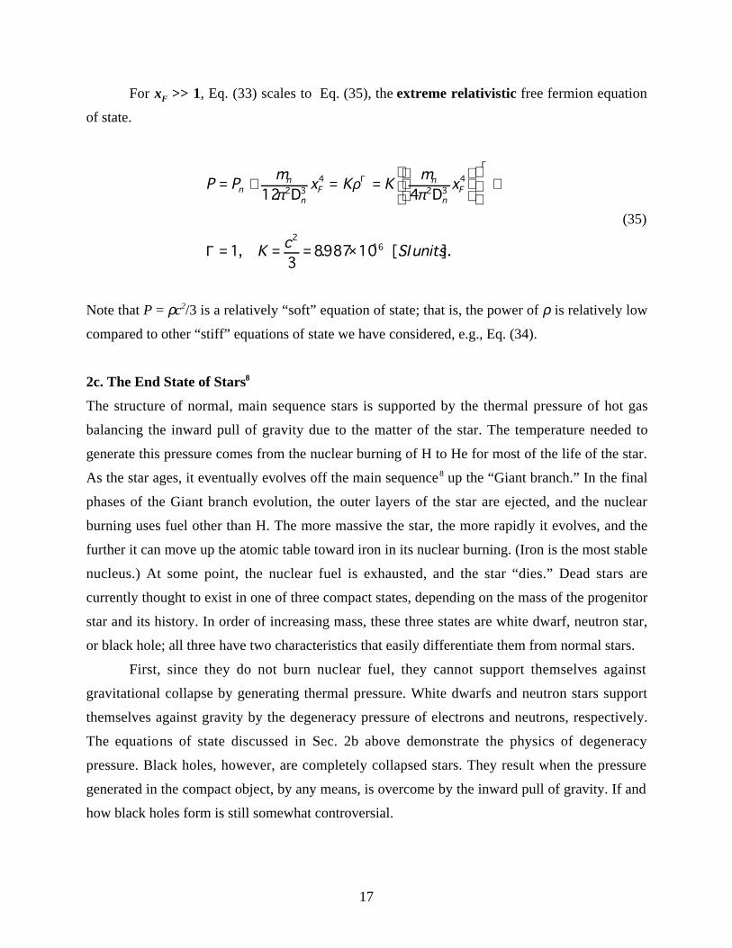
For xF >> 1, Eq. (33) scales to Eq. (35), the extreme relativistic free fermion equation
of state.
P Pm
x K Km
x
K c SI units
nn
nF
n
nF= ≅ = =
⇒
= = = ×
12 4
13
8987 10
2 34
2 34
216
πρ
πD DΓ
Γ
Γ , . [ ].
(35)
Note that P = ρc2/3 is a relatively “soft” equation of state; that is, the power of ρ is relatively low
compared to other “stiff” equations of state we have considered, e.g., Eq. (34).
2c. The End State of Stars8
The structure of normal, main sequence stars is supported by the thermal pressure of hot gas
balancing the inward pull of gravity due to the matter of the star. The temperature needed to
generate this pressure comes from the nuclear burning of H to He for most of the life of the star.
As the star ages, it eventually evolves off the main sequence8 up the “Giant branch.” In the final
phases of the Giant branch evolution, the outer layers of the star are ejected, and the nuclear
burning uses fuel other than H. The more massive the star, the more rapidly it evolves, and the
further it can move up the atomic table toward iron in its nuclear burning. (Iron is the most stable
nucleus.) At some point, the nuclear fuel is exhausted, and the star “dies.” Dead stars are
currently thought to exist in one of three compact states, depending on the mass of the progenitor
star and its history. In order of increasing mass, these three states are white dwarf, neutron star,
or black hole; all three have two characteristics that easily differentiate them from normal stars.
First, since they do not burn nuclear fuel, they cannot support themselves against
gravitational collapse by generating thermal pressure. White dwarfs and neutron stars support
themselves against gravity by the degeneracy pressure of electrons and neutrons, respectively.
The equations of state discussed in Sec. 2b above demonstrate the physics of degeneracy
pressure. Black holes, however, are completely collapsed stars. They result when the pressure
generated in the compact object, by any means, is overcome by the inward pull of gravity. If and
how black holes form is still somewhat controversial.
18
Second, white dwarfs, neutrons stars, and stellar mass black holes are very compact
objects compared to normal stars. With typical masses greater than 1 M§, and radii of 10-2 R§ for
white dwarfs, 10-5 R§ for neutron stars, and 3 (M/M§) [km] for black holes, these objects have
much smaller radii, and consequently much stronger “surface” gravitational fields than normal
stars. (Here, we are considering stellar mass objects. The statement is not true for the galactic
black holes, with masses in the range 106–1010 M§, thought to be at the center of some galaxies.)
With the exception of primordial black holes formed in the very early universe, with
masses less than 1012 kg, which would have evaporated (via Hawking’s radiation) by the present
epoch, all three types of compact objects are essentially static over the lifetime of the universe.
They are the final, and typically stable, stages of stellar evolution.
(i) White Dwarf Stars
White dwarf stars have been directly observed via their radiation in visible through UV light.
Even though they no longer burn nuclear fuel, they can be seen in these wavelengths as they are
very slowly cooling as they radiate away their residual heat (109–1010 years). Those white dwarf
stars observed in well-characterized binary systems have had mass determinations. For example,
Sirius B, perhaps the best known white dwarf star, is the binary companion to Sirius. The binary
nature of the Sirius system was first reported by F. Bessel in 1844. Sirius B was unseen with the
telescopes of that time, and its existence was based on the observations of the perturbed orbit of
Sirius. Sirius B was first seen in visible light in 1863. Modern determinations of its mass from
binary system orbit parameters give a mass of 1.003 M§. Recent satellite observations in the
ultraviolet, where white dwarfs emit most of their light, have determined the surface temperature
of Sirius B to be about 30,000 K. Using these spectral measurements, the equation for the
luminosity from blackbody emission, L R Teff= 4 2 4π σ , and the accurately known distance to the
star, the radius is determined to be 5.88 x 10³ km (= 0.0845 R§). Given its large density, ρ= 2.34
× 109 kg/m3, and consequent surface gravity, Sirius B has been used to check the gravitational
redshift predicted from GR, ∆λλ
≅GM
Rc 2. The observed gravitational redshift is usually quoted as
an equivalent Doppler shift ∆λ/λ = v/c or v = 0.6362 (M/M§)/(R/R§) km/s. This predicts 91 ± 8
km/s for Sirius B, as compared to the observed value of 89 ± 16 km (Ref. 9).
19
White dwarf stars can be modeled using classical approximations to hydrostatic
equilibrium and Newtonian gravity. This is not the case for neutron stars, which will be
discussed separately.
Consider a spherically symmetric distribution of matter that represents the white dwarf
star. The mass, m(r), interior to radius r of the star is
m r r r drdm r
drr r
r( ) ( )
( )( ).= ⇒ =∫ ρ π π ρ4 42
0
2 (36)
In Eq. (36), we assume that the bulk of the matter in the star is nonrelativistic ions. A white
dwarf star is approximately in a steady state; hence, the gravitational force balances the pressure
force at every point. This results in the nonrelativistic hydrostatic equilibrium equation
dP r
dr
Gm r r
r
( ) ( ) ( ).= −
ρ2
(37)
After some algebra, Eqs. (36) and (37) can be combined to yield
142
2
rddr
rr
dP rdr
G rρ
π ρ( )
( )( )⋅
= − . (38)
This equation takes a simple form in the case of a polytropic equation of state, Eq. (29). Writing
the polytropic exponent as Γ ≡ +11
n, where n is called the polytropic index, Eq. (38) can be
reduced to dimensionless form with the substitutions
ρ ρ θ ξρ
π= = =
+ −
cn c
n
r a with an K
G, , ,
( ) ( / )14
1 1
, (39)
where ρc = ρ (r = 0) is the central density of the white dwarf star. (K is the polytropic constant.)
Some straightforward algebraic manipulation results in the Lane-Emden equation,
20
12
2
ξ ξξ
θξ
θd
d
d
dn
= − . (40)
The boundary conditions for a polytropic star are formulated at ξ = r = 0,
θρρ
θξ
ρ
ξ
((
, .0)0)
1 00 0
= = = == =c r
d
d
d
dr (41)
Since, m r rc( ) ( / )≅ ρ π4 33 , near r = 0, Eq. (37) gives dP
dr
Grc r
≅ →→4
30
0
πρ . Then, from the
polytropic equation of state, Eq. (28), we derive the latter boundary condition of Eq. (41).
Equation (40) can be solved by integrating numerically from ξ = 0 with the boundary
conditions of Eq. (41). The solutions, θ (ξ), decrease monotonically and have a zero for n < 5 (Γ
> 6/5) at a finite value of ξ ≡ ξR. (Note that the extreme relativistic free fermion equation of state,
Eq. (35), has Γ = 1 and does not have solutions by this method.) Using Eq. (39), we find the
radius of the star to be
R = aξR , (42)
and with the help of Eq. (40), the star’s mass is
M r r dr a d ad
dcn
c
R
R
R
R
= = = − ⋅∫∫ 4 4 42 3 2 3
00
2π ρ π ρ ξ θ ξ π ρ ξθξ
ξ
ξ
( ) . (43)
ρc can be eliminated by solving Eqs. (42) and (43) in terms of M and R. This gives the mass-
radius relation for polytropes with Γ > 6/5,
M Rn K
Gdd
n
n
n
n
R
n
nR
R
= +
−
−−
−
−−
=
41
4
3
11
3
1 2ππ
ξ ξ θξ
ξ
( ). (44)
21
The two solutions of interest for white dwarf stars are10 the nonrelativistic and very relativistic
cases:
Γ
Γ
= ⇔ = = −
=
= ⇔ = = −
=
=
=
53
32
365375 271406
43
3 689685 201824
2
2
, , . , . ,
, , . , . .
n yieldingdd
n yieldingdd
R R
R R
R
R
ξ ξθξ
ξ ξθξ
ξ ξ
ξ ξ
(45)
For the high density limit for white dwarf stars, the Γ = 4/3 solution is a reasonable
approximation. Using the above numbers in Eq. (44) for the Γ= 4/3 case, with K given by
Eq. (33), we find
MY
GYe
e=× ⋅
= ⋅41243 10
2 01824) 1 210
4
3
3
2
2ππ
.( . .455( ) M§. (46)
The relation R = aξR gives
RY
GY
kg me c
ec= ⋅
× ⋅ ⋅= × ⋅ ⋅ ⋅
⋅
−
−−
−
6896851 243 10
2 231 10 210
104
3
2
34
2
310 3
1
3
.( . )
. ( )ρ
πρ
R§. (47)
For example, in the case of completely ionized pure 26Fe56 and xF = 10, we have ρ = 2.105 × 10¹²
kg/m3; this results in M = 1.253 M§ , R = 3.568 × 10⁻⁵ R§ (= 0.389 earth radii).
In Eq. (46), M is independent of R and hence ρc. This mass limit for white dwarf stars, in
the relativistic limit of Eq. (33), is called the Chandrasekhar limit, or Mch = 1.46 M§. It is the
largest possible mass of a white dwarf star. Degenerate stars of higher mass must take other
forms such as neutron stars or black holes (discussed below). Figure 3 shows an intuitive way to
understand how the Chandrasekhar limit comes about.11 The figure shows log Pc vs. log ρc for
the equation of state of white dwarf stars as the solid line. Also plotted as a dotted line is the
inward pressure of gravity at the center of the star for two stellar masses, 0.8 and 1.5 M§ (the
radius of the star is an implied variable). At lower masses, e.g., < 0.8 M§, the system is
22
nonrelativistic and Pc ∝ ρ c5/3. The slope of the equation of state in this case is larger than the
slope of the Pc vs. ρc relation from gravity, and there is a solution for ρc, Pc. There is then a
transition region that has a changing slope of Pc vs. ρc which still allows solutions. Finally, in the
very relativistic limit, Pc ∝ ρc4/3 and the slope of the equation of state is parallel to that of the Pc
vs. ρc relation from gravity. Thus, in the very relativistic case, there is no solution, and these
more massive white dwarf stars are unstable. The last mass that allows a solution is Mch, just less
than 1.5 M§. Note that it is the transition from Ee ≅ pe2/2me to Ee ≅ pe that loses a power of pe and
leads to this result. Very basic physics!
(ii) Neutron Stars
Stable degenerate stars with masses larger than Mch are constructed by using the general
relativistic Oppenheimer-Volkoff (OV) equations. The OV equations are solutions of Einstein’s
field equations describing the stellar structure for a nonrotating spherical star in hydrostatic
equilibrium (time independent). We write them in a form that resembles Eqs. (36) and (37),
dm r
drr r
( )( )= 4 2π ρ , (48)
dP r
dr
Gm r r
r
P r
r c
P r r
m r c
Gm r
rc
( ) ( ) ( ) ( )
( )
( )
( )
( )= − +
+
−
−ρρ
π2 2
3
2 2
1
1 14
12
, (49)
d
dr r
dP r
dr
P r
r c
Φ= − +
−1
12
1
ρ ρ( )
( ) ( )
( ). (50)
Baad and Zwicky12 invented the idea of a “neutron star” and predicted that neutron stars
are the remnants of supernovas. They did not make quantitative calculations but estimated that
neutron stars would have a very small radius and high density. The first actual model calculation
of neutron star properties was made by Oppenheimer and Volkoff.13 They solved the OV
equations assuming an ideal relativistic gas of free neutrons as the equation of state, cf. Eq. (35).
Neutron stars are thought to form when the Fermi sea of electrons of the ionized matter in
a white dwarf configuration fills beyond the energies available to β decay. This happens in the
extreme relativistic electron limit, i.e., very high density. With the Fermi levels filled beyond the
23
energy of the electrons from neutron-beta decay, there is “no place for these electrons to go,” and
inverse β decay is favored. This causes a “neutron drip” above a central density, ρc, of the star of
about 4 × 10¹⁴ kg/m3. (Note that ρnuc ≅ 3 × 10¹⁷ kg/m3.) The neutron star is an exotic regime of
matter that is not well understood. For white dwarf stars, observations of masses and radii are
used as evidence for the confirmation of the stellar models. In the case of “neutron stars,”
because of the lack of experimental knowledge about the equation of state at these extreme
conditions, observations of masses and radii are used as a probe of this exotic state of matter.
Figure 4 shows the various stages of degenerate stars in neutron star models14 that were
developed in the 1950s–1970s. These “nuclear” models assume extrapolations of simple low-
energy nuclear physics to “nuclei” of > 1057 nucleons, and ρc >> ρnuc . I will argue below, when I
discuss strange stars and Q-stars, that this may not be valid. The upper right hand corner shows a
stability diagram of mass vs. ρ c. The regions where d m/dρc > 0 are generally stable. For
ρc < 1012 kg/m3, stable white dwarf stars exist. For 2 × 10¹⁶ < ρc < 5 × 10¹⁸ kg/m3, nuclear models
indicate that neutron stars exist. Above this density range, there is great uncertainty of what
states of matter might exist; however, the current consensus is that total gravitational collapse of
the star occurs into a black hole above some limiting mass.
About 17 binary star systems containing at least one neutron star candidate have yielded
good mass estimates of the neutron star(s). (How this measurement is made is discussed in
Sec. 3b below.) All of these neutron star mass values lie in the range 1.35 ± 0.27 M§ (Ref. 15)
and are consistent with mass estimates from a number of nuclear neutron star models.
The possibility of identifying heavier compact objects as black holes relies, almost
entirely, on being able to state categorically that the observed object has a mass larger than the
maximum allowed mass of the heaviest stable compact stellar object. Conventional wisdom
identifies the heaviest stable compact stellar objects as neutron stars described by nuclear
models. In this approximation, we find a reasonably firm upper limit on the mass of a neutron
star. Below, I reproduce the assumptions of Rhoades and Ruffini16 as I have quibbles about some
of these that will become important when we discuss Q-stars. In our discussion of mass limits,
initially we assume no rotation. As it turns out, rotation adds at most 20% to the mass limit as
compared to no rotation.
Rhoades and Ruffini made the following set of assumptions in their derivation of the
mass limit of neutron stars.
24
A. General relativity is the correct theory of gravity, and thus the OV equations determine the
equilibrium structure of the compact object.
B. The equation of state satisfies the “microscopic stability” condition, dP/dρ ≥ 0. If this
condition were violated, small elements of nuclear matter would spontaneously collapse.
C. The equation of state satisfies the causality condition, dP/dρ ≤ c2; that is, the speed of sound
in the neutron star is bounded by the speed of light in vacuum.
D. The equation of state below a matching density, ρmat = 5 × 10¹⁷ kg/m3, is known (ρnuc ≅ 3 ×
1017 kg/m3).
E. The equation of state corresponds to a gravitationally bound compact object; that is, the
stability of the compact object is provided by the attraction of gravity. (This is an implicit
assumption of Rhoades and Ruffini.)
This set of assumptions yields an upper limit for the neutron star mass of about 3.6 M§ (Ref.17).
Rotation brings this limit to about 4.3 M§.
(iii) Strange Stars, Q-Stars, and Black Holes
There is a theoretical class of compact objects that are not really covered by assumptions D and
E above. For this class of objects, examples of which are “strange stars” and “Q-stars,” the
equation of state is very different from those we have considered to this point because these
(theoretical) systems do not need gravity to stabilize them. These are N-body systems that have a
stable phase for bulk matter that dominates the gravitational attraction, even up to a limit of
1000 M§ in some models. These models are derived as approximate solutions to effective
Lagrangian field theories. The nuclear approximation to the equation of state we have been
considering above also originates in an effective field theory. In this case, one has an effective
Lagrangian field theory with nucleons as the fundamental fermionic field and, in simplest
approximation, pions as the force field. This approximation is the meat of theoretical nuclear
physics. However, what effective field theory might best approximate reality for M >> Mnucleus
(like 1057 nucleon masses) is not well understood. For ρc > ρnuc, a quark phase should certainly
play a role. However, even well below ρnuc, new phases of nuclear matter, which do not manifest
themselves in the nuclear physics regime, might exist that gain stability for bulk matter from the
nuclear force, not gravity.18 This latter possibility has been shown to be consistent with nuclear
physics data.19
25
I will give only a brief review of this approach in these lectures.20 In these models, a low-
energy effective field theory is used to describe a relativistic Fermi gas of quarks for strange
matter stars or nucleons, and for Q-stars bound within a finite volume. For both models, the
Lagrangian density has the form
L [ ]= / − − / + − +Ψ Ψi m g V U m V VV V∂ σ ∂ σ σµ µµ( ) ( ) ( )
1
2
1
22 2 , (51)
where Ψ is a fermion field, representing quarks for strange star matter, and nucleons for Q-star
matter, and σ and V are effective scalar and vector fields, respectively. The scalar field, σ, has an
effective potential U(σ) and generates an effective fermion mass m(σ). The vector field, V, has
effective mass mV and effective coupling gV. In solving the above equation, we neglect the
dynamics of the vector field. In many cases in the literature, the vector field contribution is
neglected completely, and the operational equation becomes
L [ ]= / − + −Ψ Ψi m U∂ σ ∂ σ σµ( ) ( ) ( )1
22 . (52)
These equations are solved semiclassically. Only the Pauli exclusion principle for the fermions is
treated quantum mechanically.
In the applications we are considering, this theory is used to describe a relativistic Fermi
gas of quarks or nucleons bound within a finite region of space, i.e., a spherically symmetric
compact stellar object. Including the vector repulsion between fermions, the Fermi sea is
described by the Fermi momentum, kF, and Fermi energy, EF,
E k mk
F FV F= + +2 2
3
3 3
απ
, απV
V
V
g
m=
32
, (53)
where the parameter αV gives the strength of the repulsive fermion (vector) interaction.
In this model, we take U(σ) such that inside the bulk of the star, σ takes on a constant
value, σ = σinside. The star has a very thin surface region, where σ undergoes rapid transition to a
different constant vacuum value, σ = σvacuum.
26
In the approximation of chiral symmetry for the hadronic matter of the star, the fermions
are massless inside the star, and m(σinside) = 0 (m(σvacuum) = Mnucleon). More generally, for this type
of matter, m(σinside) < Mnucleon. This can result in a more energetically favorable configuration, i.e.,
a bound system, if the fermion energy inside the star is lower than that of free fermions by an
amount greater than the gain in scalar field potential energy. (Note that we have not mentioned
gravity yet.)
In the chiral symmetry case, including nondynamical effects of the vector field V, the
equation of state is
ρ α ρ− − + − − =3 4 2 00 0
3
2P U P UV ( ) , U U inside0 ≡ ( ).σ (54)
In these models, the hadronic matter is a perfect fluid with the number of fermions > 1057. Thus,
gravity can be important and the OV equations are used in the formulation of the problem. These
can be integrated using Eq. (54). The compact star boundary conditions define the stellar surface
at the radius where the total hadronic pressure, PΨ--U0, vanishes. (Note that P in Eq. (54)
includes effects from gravity as well as hadronic pressure.)
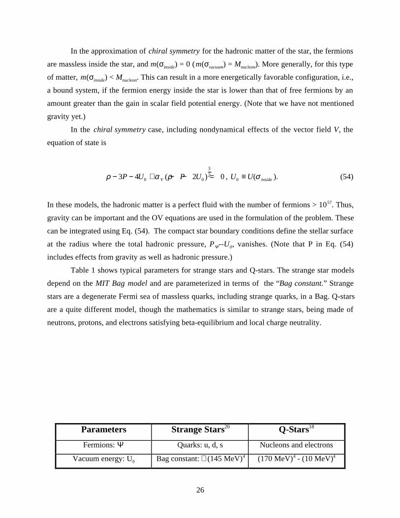
Table 1 shows typical parameters for strange stars and Q-stars. The strange star models
depend on the MIT Bag model and are parameterized in terms of the “Bag constant.” Strange
stars are a degenerate Fermi sea of massless quarks, including strange quarks, in a Bag. Q-stars
are a quite different model, though the mathematics is similar to strange stars, being made of
neutrons, protons, and electrons satisfying beta-equilibrium and local charge neutrality.
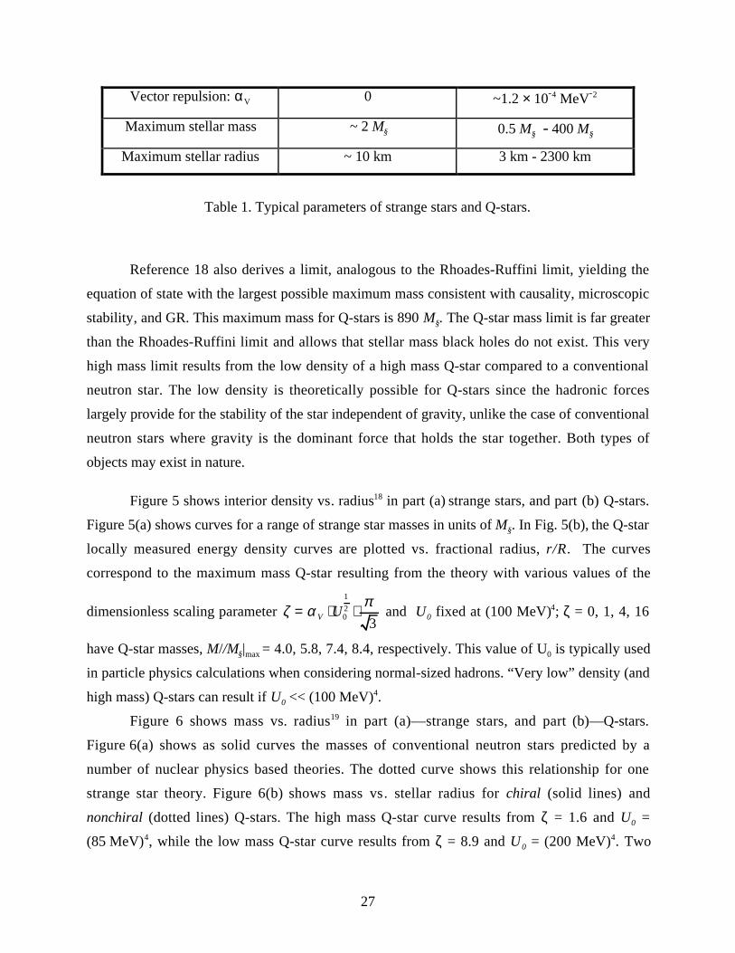
Parameters Strange Stars20 Q-Stars18
Fermions: Ψ Quarks: u, d, s Nucleons and electrons
Vacuum energy: U0 Bag constant: ≅ (145 MeV)4 (170 MeV)4 - (10 MeV)4
27
Vector repulsion: αV 0 ~1.2 × 10⁻⁴ MeV-2
Maximum stellar mass ~ 2 M§ 0.5 M§ - 400 M§
Maximum stellar radius ~ 10 km 3 km - 2300 km
Table 1. Typical parameters of strange stars and Q-stars.
Reference 18 also derives a limit, analogous to the Rhoades-Ruffini limit, yielding the
equation of state with the largest possible maximum mass consistent with causality, microscopic
stability, and GR. This maximum mass for Q-stars is 890 M§. The Q-star mass limit is far greater
than the Rhoades-Ruffini limit and allows that stellar mass black holes do not exist. This very
high mass limit results from the low density of a high mass Q-star compared to a conventional
neutron star. The low density is theoretically possible for Q-stars since the hadronic forces
largely provide for the stability of the star independent of gravity, unlike the case of conventional
neutron stars where gravity is the dominant force that holds the star together. Both types of
objects may exist in nature.
Figure 5 shows interior density vs. radius18 in part (a) strange stars, and part (b) Q-stars.
Figure 5(a) shows curves for a range of strange star masses in units of M§. In Fig. 5(b), the Q-star
locally measured energy density curves are plotted vs. fractional radius, r/R. The curves
correspond to the maximum mass Q-star resulting from the theory with various values of the
dimensionless scaling parameter ζ απ
= ⋅ ⋅V U0
1
2
3 and U0 fixed at (100 MeV)4; ζ = 0, 1, 4, 16
have Q-star masses, M//M§|max = 4.0, 5.8, 7.4, 8.4, respectively. This value of U0 is typically used
in particle physics calculations when considering normal-sized hadrons. “Very low” density (and
high mass) Q-stars can result if U0 << (100 MeV)4.
Figure 6 shows mass vs. radius19 in part (a)––strange stars, and part (b)––Q-stars.
Figure 6(a) shows as solid curves the masses of conventional neutron stars predicted by a
number of nuclear physics based theories. The dotted curve shows this relationship for one
strange star theory. Figure 6(b) shows mass vs. stellar radius for chiral (solid lines) and
nonchiral (dotted lines) Q-stars. The high mass Q-star curve results from ζ = 1.6 and U0 =
(85 MeV)4, while the low mass Q-star curve results from ζ = 8.9 and U0 = (200 MeV)4. Two
28
conventional neutron star models, plotted as dashed lines, are shown for comparison.
Figures 5(b) and 6(b) show that it is easy to obtain Q-star masses that exceed the Rhoades-
Ruffini limit for neutron stars; however, strange star masses and radii are predicted to be very
close to those of conventional neutron stars for M/M§ > 0.5.
(iv) Summary
In the above sections, we have briefly reviewed white dwarf stars, conventional neutron stars,
and some unconventional stellar models, e.g., strange stars and Q-stars. White dwarf stars are
well established experimentally by direct observation from ground- and space-based telescopes.
There is very good agreement between extensive experimental data and theory. Neutron stars are
less well understood as the experimental information about them is essentially limited to mass
determinations, pulsar periods, and spectral energy and timing information, including those
coming from space-based x-ray measurements of binary systems containing a neutron star
candidate.
Conventional theory predicts that compact stellar objects with masses greater than the
Rhoades-Ruffini limit for neutron stars must collapse into a black hole. As we shall explore later
in these lectures, this mass limit is currently the primary experimental evidence for stellar black
hole candidates. In addition, there exists spectral and timing information coming from space
based x-ray measurements of x-ray binary systems containing a black hole candidate (BHC).
The bogus observation of a submillisecond pulsar in the late 1980s seemed to challenge
the limits of rotational stability of conventional neutron stars. This stimulated theorists (for a
while) to explore other theories that could accommodate such a startling observation, based on
modern ideas in particle physics. Thus, an incorrect observation was one of the primary reasons
for the invention of strange stars and Q-stars; it had the value of forging a new direction in
theory. Unexpectedly, the theory of Q-stars had the additional important result of greatly
exceeding the Rhoades-Ruffini mass limit for neutron stars before requiring collapse to a black
hole. The Q-star mass limit is so large, at about 890 M§, that it could eliminate the practical
possibility of stellar mass black holes.
Strange stars have be invented to closely mimic neutron stars except for their ability to
spin faster. Thus for M/M§> 0.5, strange stars and neutron stars are predicted to be very close in
mass and radius. However, as Fig. 5(a) shows, below this mass range, strange stars have a much
29
smaller radius than neutron stars, and this might be a way of eventually experimentally
distinguishing them.
Q-stars can be very different from neutron stars and black holes, and offer fertile ground
for experimental observations. A Q-star having the same mass as the BHC Cygnus X-1, with
M/M§ = 16 ± 5, has a Q-star surface radius of about 80 km as compared to a black hole with a
horizon radius of about 50 km. As we will discuss in some detail further in these lectures, for
Cygnus X-1, it currently appears feasible to distinguish the Q-star and black hole hypotheses
experimentally. The search for strong additional experimental evidence, beside mass limits, for
(or against) stellar mass black holes is one of the more challenging areas of particle astrophysics.
3. Laboratories for Particle Astrophysics: X-Ray Stellar Binary Systems and
Active Galactic Nuclei (AGN)
The first priority of physics is to obtain experimental information about objects in the universe
that we wish to study. Without such experimental information, theoretical speculations can be
very misleading. The seminal questions that concern particle astrophysics require relatively new
and exploratory experimental techniques to study the exotic objects that theorists have posited
should exist. In this section, we briefly review some of the most promising of such techniques
that could yield experimental information about the nature of compact stellar objects beyond
white dwarfs, and their relationship to gravity. In particular, experimental “proof” of the
existence or nonexistence of black holes is central to this effort. In this case, “what is involved is
not just the investigation of yet another, even if extremely remarkable, celestial body, but a test
of the correctness of our understanding of the properties of space and time in extremely strong
gravitational fields.”2
3a. Description of X-Ray Binary Systems
An x-ray binary system is characterized by an optically (and radio) visible star orbiting about an
optically (and radio) invisible compact stellar object. However, the close environment of the
compact stellar object is visible in x-rays. Figure 7 shows a schematic of such an x-ray binary
system containing a BHC and an ordinary star. (Note that the figure is not to scale, with the
accretion disk/black hole actually being much smaller than shown relative to the normal star.)
Known BHC binary systems contain a stellar mass BHC with a mass in the range 3–30 M§.
Binary systems can also contain a white dwarf star or a neutron star.
30
For neutron stars and BHCs, two types of x-ray binary systems are observed, high mass
x-ray binary systems, HMXB, and low mass x-ray binary systems, LMXB. HMXB contain a
high mass supergiant star (33 M§ for Cyg X-1) and a compact object. The compact object in a
HMXB is typically a BHC, or a relatively young neutron star, which is usually a pulsar with a
large magnetic field of ~ 108 T. LMXB systems contain a low mass main sequence star of about
1 M§, and a compact object. The compact object in an LMXB is typically a BHC or a relatively
old neutron star, which has a reduced magnetic field of ~ 104 T and does not show pulsation.
The phenomenology of these systems is discussed in Sec. 4a.
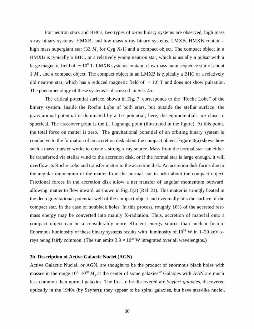
The critical potential surface, shown in Fig. 7, corresponds to the “Roche Lobe” of the
binary system. Inside the Roche Lobe of both stars, but outside the stellar surface, the
gravitational potential is dominated by a 1/r potential; here, the equipotentials are close to
spherical. The crossover point is the L1 Lagrange point (illustrated in the figure). At this point,
the total force on matter is zero. The gravitational potential of an orbiting binary system is
conducive to the formation of an accretion disk about the compact object. Figure 8(a) shows how
such a mass transfer works to create a strong x-ray source. Mass from the normal star can either
be transferred via stellar wind to the accretion disk, or if the normal star is large enough, it will
overflow its Roche Lobe and transfer matter to the accretion disk. An accretion disk forms due to
the angular momentum of the matter from the normal star in orbit about the compact object.
Frictional forces in the accretion disk allow a net transfer of angular momentum outward,
allowing matter to flow inward, as shown in Fig. 8(a) (Ref. 21). This matter is strongly heated in
the deep gravitational potential well of the compact object and eventually hits the surface of the
compact star, in the case of nonblack holes. In this process, roughly 10% of the accreted rest-
mass energy may be converted into mainly X-radiation. Thus, accretion of material onto a
compact object can be a considerably more efficient energy source than nuclear fusion.
Enormous luminosity of these binary systems results with luminosity of 1031 W in 1–20 keV x-
rays being fairly common. (The sun emits 3.9 × 1026 W integrated over all wavelengths.)
3b. Description of Active Galactic Nuclei (AGN)
Active Galactic Nuclei, or AGN, are thought to be the product of enormous black holes with
masses in the range 106–1010 M§ at the center of some galaxies.22 Galaxies with AGN are much
less common than normal galaxies. The first to be discovered are Seyfert galaxies, discovered
optically in the 1940s (by Seyfert); they appear to be spiral galaxies, but have star-like nuclei.
31
Their optical emission spectra are quite different from normal galaxies. The next class of AGN
to be discovered were a subclass of radio galaxies. By the mid-1950s, it was known that radio
galaxies were sources of very large fluxes of high-energy particles and had very strong magnetic
fields. A few of these had prominent star-like nuclei in the optical and were called N-galaxies.
These were similar to Seyfert galaxies in their emission spectra. However, the relationship
between Seyfert and N-galaxies was not clear at that time.
In the 1960s, quasars were discovered by Martin Schmit. In 1962, he found that the
strong radio source and quasistellar object, 3C 273, has a redshift of z = ∆λ/λ = 0.158, which,
according to Hubble’s law, places it at about 2 × 10⁹ light years away (H0 = 50 km/s/Mpc). The
observed luminosity of 3C 273 implied an intrinsic luminosity in the visible and radio
frequencies for the object of more than 103 times that of the entire Milky Way galaxy (our galaxy
that has a luminosity of 2 × 10¹⁰ L§ = 8 × 1036 W). Besides having the appearance of a point
object in the photographs, the quasar varied noticeably in brightness. Following this discovery,
many more quasars were found, all of them characterized by strong radio emission, stellar
appearance, and very great distances. Soon after, radio-quiet quasars were discovered. They are
similar to radio-loud quasars in the optical range but are relatively weak sources of radio
emission. Quasars are among the most energetic examples of AGN known. Optical observation
of relatively close quasars show that the source of the very strong optical emission is the nucleus
of a galaxy.
Some of the most energetic examples of AGN are the BL Lacertae, or BL-Lac, objects,
and the rapidly variable (in the optical, x-ray, and gamma-ray) quasars called blazars. These are a
subset of the quasars and demonstrate variability in luminosity on timescales of hours to days,
depending on the wavelength. This implies that the source of this radiation must be quite
compact. In the case of BL-Lac objects, the optical spectra are normally featureless and the
continuum radiation is strongly polarized. They also show strong x-ray and very strong gamma-
ray emission to tens of GeV. It is plausible that for BL-Lac objects, we are directly observing the
primary source of energy from the AGN.
We now have a model of AGN that can qualitatively explain the observations described
above. In this model, the AGN is powered by a massive black hole with masses in the range 106–
1010 M§ at the center of a galaxy. Figure 8(b) shows the energy flow from the AGN. The black
hole, by a mechanism that is not completely understood at this time, generates two opposing jets
of relativistic plasma and radiation that are highly collimated via relativistic beaming. These jets
32
are the source of the gamma-rays, and eventually, the strong radio signals seen. The inner edge
of the accretion disk is the main source of x-rays, and also provides the material flow to the jets.
Figure 9(a) shows a ground-based superimposed optical-radio image of the galaxy NGC 4261,
which contains an AGN. Notice the scale on the figure. The galaxy is an elliptical with two jets
of material emanating from its core region. The jets in part (a) of the figure are the source of very
strong radio signals. The core of the galaxy is exposed in Fig. 9(b), showing a Hubble Space
Telescope23 image of the central region of the galaxy with the radio jets superimposed (not to
scale) for orientation. This image was taken before the Hubble was repaired. The disk-like
structure seen in the figure is not an accretion disk as it does not show the differential rotation as
a function of r necessary to transfer material in towards the center. Spectroscopic observations of
this disk structure indicate that it is rotating as a solid body. The actual AGN region is contained
in the bright dot in the center of the hole in the “donut” and is not resolved in this picture.
Subsequent pictures with Hubble after its repair have left open the question of the nature of the
central region of this AGN. There is currently no direct experimental evidence for a black hole at
the center of NGC 4261. However, we might speculate, and Fig. 9(c) shows the resulting model
of what the central region might look like.
The model of an AGN shown in Figs. 8(b) and 9 allows a natural explanation of many of
the phenomena observed in AGN and unifies the observations of the various types of AGN. A
Seyfert galaxy is an evolved quasar. A quasar is a particularly powerful AGN, the large distance
to the quasar dimming the rest of the galaxy. Radio-loud AGN galaxies have the orientation of
the jets to the earth, maximizing the radio transmission from the galaxy, while radio-quiet AGN
galaxies are oriented too poorly to transmit to Earth. Blazars are oriented with the jets from the
AGN pointing at the earth. In this way, we “see” right into the center of the AGN. Finally, the
rapid variability of AGN is due to the compact black hole “engine” at their centers. This all
seems to hang together; however, the model of super massive black holes as the driving engine
of AGN is still controversial and has only indirect experimental evidence supporting it.
3c. X-Ray Binary System Orbital Parameters
Figure 10 shows a schematic of an x-ray binary system as viewed parallel to the orbital plane. In
the figure,
• MX = mass of x-ray source (compact object)
• Mopt = mass of optical companion (normal star)
33
• q = Mop t/MX
• i = orbital plane inclination angle, where the z′ direction is to the observer
• a = ax + aopt
• ax = semimajor axis of the x-ray source
• aopt = semimajor axis of the optical companion.
Figure 11 defines an x-ray binary system’s orbital parameters. Referring to this figure:
• Periastron = position along the optical companion’s orbit nearest to the x-ray source
• φ = angle of the optical companion from the periastron, measured in the orbital plane
• Line of nodes = common x and x′ axis, defined by the line of intersection of the orbital plane
and projected observation plane, where the projected observation plane is perpendicular to
the z′ direction
• i = orbital plane inclination angle
• ω = angle of periastron from the line of nodes, measured in the orbital plane
• e = eccentricity of the optical companion’s orbit
• P = period of the binary system orbit.
In order to determine the values of the above defined parameters, we measure two observable
quantities: the intensity of the light emitted by the optical companion as a function of time (i.e.,
the binary system’s light curve) and the Doppler shift of the light emitted by the optical
companion as a function of time. (Note that “light” is really electromagnetic radiation, as radio
Doppler measurements and x-ray eclipses also yield information about binary system
parameters.)
The Doppler shift is given by
λλ
ββ
β0
1
1=
+−
= ′,v
czopt
, (55)
where vzopt′ is the velocity of the optical companion projected along the z′ axis, called the “radial
velocity.” Defining
34
10
+ =zλ
λ, (56)
Eq. (55) can be solved for the radial velocity,
v czzz
opt′ =
+ −+ +
( )( )1 11 1
2
2 . (57)
We can relate the physical observables to the orbital parameters of the x-ray binary system in a
few ways. An FFT (Fast Fourier Transform) of the binary system “light” curve may yield the
period of the binary system. The source of the information may either be eclipses of the x-ray
source by the optical companion, which gives information in the x-rays from the compact object,
or ellipsoidal variations in the optical light curve due to tidal deformations in the optical
companion from gravitational interaction with the compact object. In order to get x-ray eclipse
information, the orientation of the binary system orbital plane must be nearly parallel to the line
of sight from the earth to the binary system (depending on the geometry of the binary system,
and the size of the compact object and optical companion).
We can also use the Doppler shift data to determine the orbital parameters. The radial
velocity of the optical companion is related to its orbital parameters by its equations of motion
ψ ω φφ
( ) ( ), ( )( )
cos ( )t t r t
a e
e topt
opt
≡ + =−
+1
1
2
. (58)
These equations and the orbital definitions give
v i r rzopt opt opt′ = +sin (& sin &cos )ψ ψ ψ . (59)
Kepler’s second Law, with ropt eliminated by substitution of Eq. (58), is
& ( cos )φ
π φ=
+
−
2 1
1
2
3 2
e
P e. (60)
35
Substituting Eqs. (58) and (60) into (59) gives
[ ]v K t e P e Ka i
P ezopt opt opt
opt
′ = + + ≡−
cos( ( , , )) cos ,sin
ω φ ωπ2
1 2 . (61)
Kopt is called the semiamplitude of the optical radial velocity curve.
Figure 12 shows data from the binary system V404 Cyg. Radial velocity (km/s), obtained
from the Doppler shift data through Eq. (57), is plotted as a function of orbital phase (rad),
assuming a periodic variation. P for the system is obtained from this curve. From vmax/min, we find
from Eq. (61)
v K ev v
K
v vK e v
v v
v ve
opt opt
opt
max/ minmax min
max min max min
max min
( cos ), ,
cos , cos
= ± +−
=
+ = ≡ +−
=
12
2
ω
ω ω. (62)
Integrating the data of Fig. 12 in two ways then yields another relation between orbital
parameters,
A v v dt where v v v vzopt
v
v
1 2 1 2
1 2
, max min( ) , , ..
≡ − = =′∫ (63)
Equation (63) is related to the orbital parameters by
22 1
2 1
v v
v v
A A
A Ae
max min
max min
sin−
⋅+−
= ω . (64)
Equations (62) and (64) then solve the orbital parameters, Kopt, e, and ω in terms of radial
velocity data.
P, Kopt, e, and ω can be used to determine limits on the x-ray source’s mass. Combining
Kepler’s third law,
36
PG M M
aX opt
22
32=
+( )
( )
π, (65)
where G is Newton’s gravitational constant, with the definition of Kopt, Eq. (61), and moving all
orbital parameters of the optical companion to one side of the equation, we find
( ) sin
( )( ),
K P e
G
M i
qf M
optX
3 23 3
2
1
2 1
⋅ ⋅ −=
+≡
π(66)
where f(M) is called the optical mass function. The value of f(M) for an x-ray binary system,
which depends on readily determined orbit parameters of the optical companion, gives a lower
limit to the x-ray source’s mass, since sin3i/(1+q)2 < 1; that is,
MX > f(M). (67)
3d. Using Orbital Parameters to Determine Compact Object Masses
In the following sections, we show applications of the techniques developed in Sec. 3c. These
spectral/mechanical methods are currently the most reliable way to determine the mass of a
compact object. Section (i) shows mass solutions for stellar mass objects, while Sec. (ii)
discusses an AGN solution.
(i) Some Leading Stellar Black Hole Candidates
Figure 13 shows the orbit solutions for a number of x-ray binary systems thought to contain a
black hole as the x-ray source. The primary reason that a BHC is preferred for these systems is
the high mass of the x-ray source in these solutions compared to the Rhoades-Ruffini mass limit
for neutron stars. Later in these lectures, we will discuss information coming from the x-ray
spectra of these objects that puts them in a common category. In particular, the millisecond and
submillisecond time variability of these x-ray sources can yield important information about their
structure. For all but one of the cases, V404 Cyg, the optical mass function is less than the
Rhoades-Ruffini mass limit. However, additional information about these systems allows a
unique mass determination for the optical companion and x-ray source. The figure shows these
37
values of MX and Mopt in the two lobes of the binary system cartoons. In general, these values
are model dependent and do not have the reliability of f(M) which is also shown in the figure for
each system as is the orbital period.
(ii) The Black Hole Candidate in the AGN of M87
Though observations of the central region of NGC 4261, discussed in Sec. 3b, have not yet
provided strong experimental evidence of a massive black hole, observation of the giant elliptical
galaxy M87 has recently been more fruitful. M87 is a nearby galaxy in the Virgo cluster at a
distance of about 15 Mpc. It is a large elliptical galaxy that is a strong radio source with an AGN
and a mass of about 40 × 1011 M§, or about 20 times the Milky Way. Figure 14(a) shows a recent
NASA Hubble Space Telescope image24 of a spiral-shaped disk of hot gas in the core of the
AGN of M87. This galaxy has long been a favorite choice for seeking further evidence that radio
ellipticals have central engines fed by a surrounding disk. The powerful optical synchrotron jet,
nonthermal radio source, and large velocities of ionized gas in its nucleus singled out M87 as one
of the earliest examples of a galaxy with an AGN. The bright streak of light moving from the
center of the galaxy, at about 45° clockwise from 12 o’clock in the figure, is the optical
synchrotron jet of high-energy particles thought to be powered by the central engine of the AGN.
This photograph was taken after the December 1993 repair of the Hubble telescope.
Spectroscopic observations of ionized gas in circular motion close to the nucleus of M87
can provide a powerful and straightforward way to look for the Keplerian rotation curve, which
could be a signature of a massive black hole. The dynamics of the millions of stars, gas, and dust
in the neighborhood of the galactic nucleus is much more complex than that of a simple stellar
binary system; however, a massive central black hole will affect the kinematics of this ensemble
by producing a rapidly rotating accretion disk containing stars, gas, and dust, centered on the
black hole. Consequently, the HST team took narrow band visual images of M87 to look for such
an organized structure in the ionized gas. These images, particularly Fig. 14(b) which shows an
enlargement of the central accretion disk feature, indicate that the ionized gas in the nucleus has
indeed settled into a rotating disk. If this is true and there is a massive black hole in the center,
the rotation velocity in the disk will rise toward the center rather than decrease to zero as in a
galaxy with no central mass.
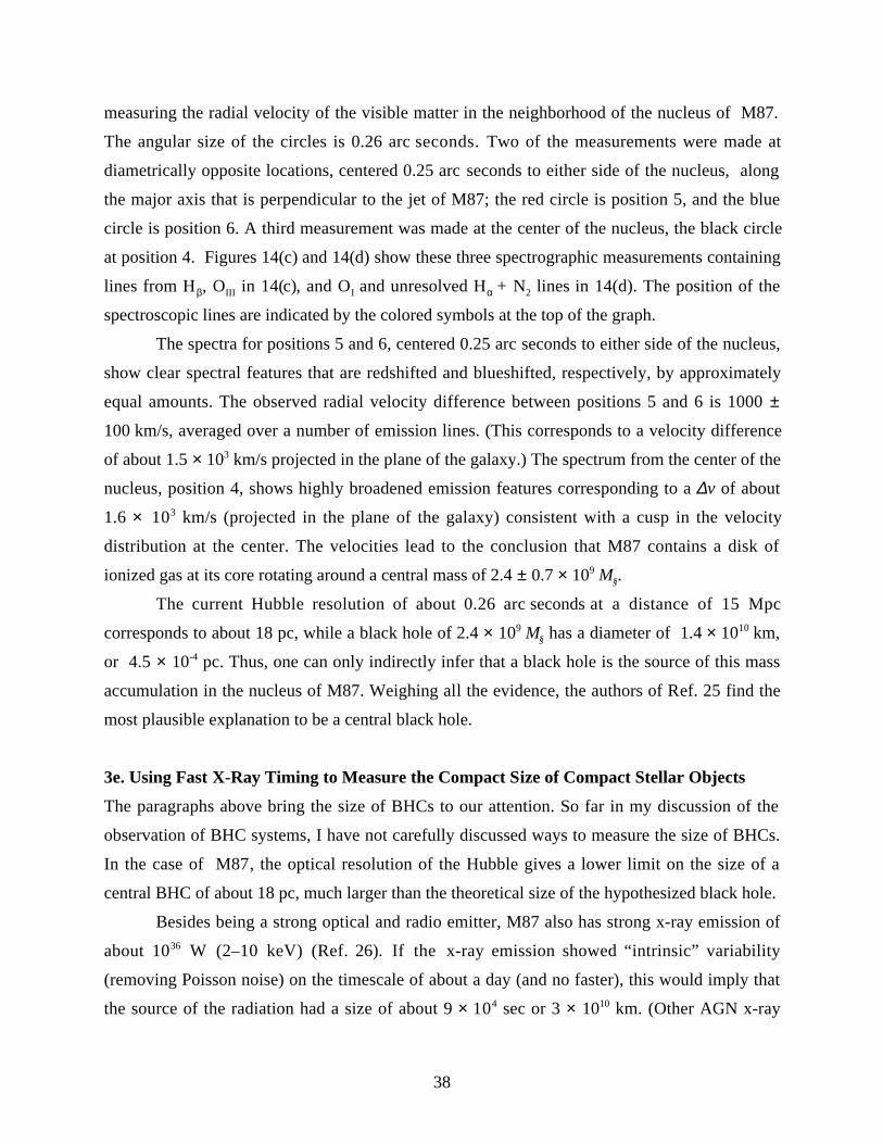
Figure 14(b) shows an enlargement of the central accretion disk feature, and the six
locations (small circles in the figure) where HST spectrographic observations25 were made
38
measuring the radial velocity of the visible matter in the neighborhood of the nucleus of M87.
The angular size of the circles is 0.26 arc seconds. Two of the measurements were made at
diametrically opposite locations, centered 0.25 arc seconds to either side of the nucleus, along
the major axis that is perpendicular to the jet of M87; the red circle is position 5, and the blue
circle is position 6. A third measurement was made at the center of the nucleus, the black circle
at position 4. Figures 14(c) and 14(d) show these three spectrographic measurements containing
lines from Hβ, OIII in 14(c), and OI and unresolved Hα + N2 lines in 14(d). The position of the
spectroscopic lines are indicated by the colored symbols at the top of the graph.
The spectra for positions 5 and 6, centered 0.25 arc seconds to either side of the nucleus,
show clear spectral features that are redshifted and blueshifted, respectively, by approximately
equal amounts. The observed radial velocity difference between positions 5 and 6 is 1000 ±
100 km/s, averaged over a number of emission lines. (This corresponds to a velocity difference
of about 1.5 × 10³ km/s projected in the plane of the galaxy.) The spectrum from the center of the
nucleus, position 4, shows highly broadened emission features corresponding to a ∆v of about
1.6 × 10³ km/s (projected in the plane of the galaxy) consistent with a cusp in the velocity
distribution at the center. The velocities lead to the conclusion that M87 contains a disk of
ionized gas at its core rotating around a central mass of 2.4 ± 0.7 × 10⁹ M§.
The current Hubble resolution of about 0.26 arc seconds at a distance of 15 Mpc
corresponds to about 18 pc, while a black hole of 2.4 × 10⁹ M§ has a diameter of 1.4 × 10¹⁰ km,
or 4.5 × 10⁻⁴ pc. Thus, one can only indirectly infer that a black hole is the source of this mass
accumulation in the nucleus of M87. Weighing all the evidence, the authors of Ref. 25 find the
most plausible explanation to be a central black hole.
3e. Using Fast X-Ray Timing to Measure the Compact Size of Compact Stellar Objects
The paragraphs above bring the size of BHCs to our attention. So far in my discussion of the
observation of BHC systems, I have not carefully discussed ways to measure the size of BHCs.
In the case of M87, the optical resolution of the Hubble gives a lower limit on the size of a
central BHC of about 18 pc, much larger than the theoretical size of the hypothesized black hole.
Besides being a strong optical and radio emitter, M87 also has strong x-ray emission of
about 1036 W (2–10 keV) (Ref. 26). If the x-ray emission showed “intrinsic” variability
(removing Poisson noise) on the timescale of about a day (and no faster), this would imply that
the source of the radiation had a size of about 9 × 10⁴ sec or 3 × 10¹⁰ km. (Other AGN x-ray
39
sources show variability on timescales as short as hours.) Such an observation would then imply
that an object about the size of a 2.4 × 10⁹ M§ black hole was the source of the radiation, and so
add much more credence to the black hole hypothesis. Unfortunately, no such evidence of x-ray
variability currently exists for M87. However, when there is variability, the technique of using x-
ray timing measurements is a powerful way to estimate the size of compact objects.
(i) X-Ray Timing Measurements for Cyg X-1
Cyg X-1 (cf. Fig. 13) is a binary star system containing an optically visible ninth magnitude
supergiant B star and an unseen companion. As discussed in Sec. 3d(i), the mass estimate for the
B star is 33 M § and for the unseen companion 16 M§. It is this large mass of the unseen
companion that qualifies it as a BHC. The system has an accretion disk about the unseen
companion that is the source of the x-rays, and it is fed by matter infall from the B star. Before
discussing the x-ray timing measurements that give evidence to the very compact size of the
unseen companion in the Cyg X-1 system, we need a bit more theoretical background.
In general relativity (GR), the effective potential V for a test particle of mass m and
angular momentum L in the Schwarzschild geometry of a concentrated mass M is27
V m M r L mr= − ⋅ +( / ) [ /( ) ]1 2 1 2 2 , (68)
where the effective potential is defined by
m dr d V r E2 2 2 2( / ) ( )τ + = . (69)
E is the energy of the particle, and τ is the proper time.
Figure 15 shows V/m, the effective potential profile, and E/m, various energies of the
system shown as the two horizontal lines and the five dots, vs. r/M for various angular momenta,
L M/ , where L L m= / . The Newtonian approximation for the case L M/ .= 433 is shown as
the dashed line to be compared to the exact GR solution. In the asymptotic limit, r/M → ∞, GR
tends to the Newtonian approximation.
40
The figure shows effective potential profiles for nonzero rest-mass particles with L M/
between 4.33 and 3.464 = 2 3+ ε, orbiting a Schwarzschild black hole of mass M. The lines
correspond to particles with stable bound orbits; the dots correspond to particles with stable
circular orbits. Such orbits only exist for L M/ > 2 3. For smaller L M/ , the orbit becomes
unstable, and the particle will always fall into the black hole. The radius of this last stable
circular orbit is rls= 6M, and the energy per unit mass of a particle in the last stable circular orbit
is 5.72%. (Remembering that Rsch ≡ 2GM/c2 = 2M ≅ 3(M/M§) [km], rls= 3Rsch ≅ 9(M/M§)[km].)
Thus, a particle starting far from the black hole with little energy gains 5.72% of its rest mass by
the time it has spiraled into the innermost stable orbit about the hole. This conversion of rest
mass to other forms of energy has much greater yield than does nuclear burning, which releases a
maximum of 0.9% of the rest mass (H → Fe).
Now back to the Cyg X-1 system. Generally, the accretion process generates rapid and
violent fluctuations in x-ray luminosity. Observations and models indicate fluctuations on a
broad range of timescales. Several accretion disk models of binary systems containing a black
hole, with the general properties of the Cyg X-1 system, indicate that a large fraction of the x-ray
luminosity from the system originates in the region of the inner edge of the disk, which is
defined by rls. In analyzing the time series of x-ray counts coming from Cyg X-1, one would then
expect to observe fluctuations on a broad range of timescales, with a cut-off in x-ray power at the
timescale corresponding to the innermost stable orbit of the accretion disk. Naively, this would
be at ∆t ≈ 2rls/c. For the unseen companion in Cyg X-1, modeled as a black hole of mass 16 M§,
this timescale corresponds to about 1 ms.
A measurement of the timescale of this cut-off has been made by the HEAO A-1
experiment.28 Figure 16(a) shows the HEAO satellite, which had a complement of four major
experiments designed to observe astronomical sources in the low energy x-ray to low energy
gamma-ray spectral region. Figure 16(b) shows the A-1 experiment in some detail. This
experiment was built by NASA and NRL, and was designed to be a survey instrument sensitive
to x-rays in the 1–30 keV energy band.29 It was operational during the years 1977–1979. The
experiment is basically a collimated thin-window multiwire proportional chamber array, with a
net aperture of about 1 m2. The angular acceptance (FWHM) of the collimators is given in the
figure, with each proportional chamber module, 1–7, having the x × z acceptance printed on it.
The long direction of collimation is parallel to the long direction of the module (along the x-
axis). Much of the time, while in the survey mode, the HEAO satellite was spinning about the z-
41
axis (which points towards the sun). Typical photon timing information was at 5 ms and longer
timescales; however, a number of special telemetry runs were made with 7.8 µs timing
resolution. Unfortunately, as is often the case in space-based experiments, all did not go well.
Soon after launch, about 2/3 of the effective area was lost due to module failures (which were
never completely understood). In addition, energy pulse-height information was essentially lost
for all the data due to a serious malfunction in the ADC system. No way to drop the beam and go
into the IR to fix these problems!
On May 7, 1978, HEAO A-1 was taking pointed data on Cyg X-1 while the source was in
the “low” state (the state believed appropriate to observe the core of the x-ray source, see
Sec. 4(a). The average count rate observed by A-1 was 1020 Hz, or a mean energy flux of 1.25 ×
10-11 W/m2 integrated over the 1–30 keV range. This corresponds to a mean source luminosity of
about 1030 W in this x-ray band, using the current estimate of the distance to Cyg X-1 of 2.5 kpc.
The A-1 proportional counter detector employed for the observation had a net aperture of
1650 cm2 and a 1° × 4° (FWHM) field of view. Data were received in real time during one
HEAO pass over a ground receiving station for a total of nine minutes. During the pass, the
satellite’s 128 kbit/sec data transmission rate was used, while data were being taken by A-1 at
that same rate. (The normal A-1 data taking rate was much lower.) The data stream had a “1” or
“0” set every 7.8 µs, with a “1” indicating that at least one x-ray event had been detected in that
time interval. Note that for Poisson-distributed events of average rate 1020 Hz, the probability of
more than one event falling in a 7.8 µs interval is 8 × 10⁻³. No photon energy information was
recorded for the events in this transmission mode.
The analysis of these data to determine the intrinsic time variability of Cyg X-1 is
complicated by the purely statistical fluctuations in the x-ray luminosity. A contamination arises
at the shorter timescales from fluctuations on longer timescales “leaking” into the measured
power at shorter timescales; this statistical effect has to be unfolded from the data. The analysis
of Ref. 28 used a specially constructed algorithm to deal with this effect.
A brief description of the analysis method is as follows:
• The determination of variability on a given timescale must be measured in the presence of
other (possibly contaminating) variability timescales.
• Data (counts) from the entire nine-minute, 7.8 µs sample were sorted according to their time
of occurrence into sets with ten bins per set. This was done for a fixed bin width for all the
data. This yields many ten-bin sets over the entire data sample.
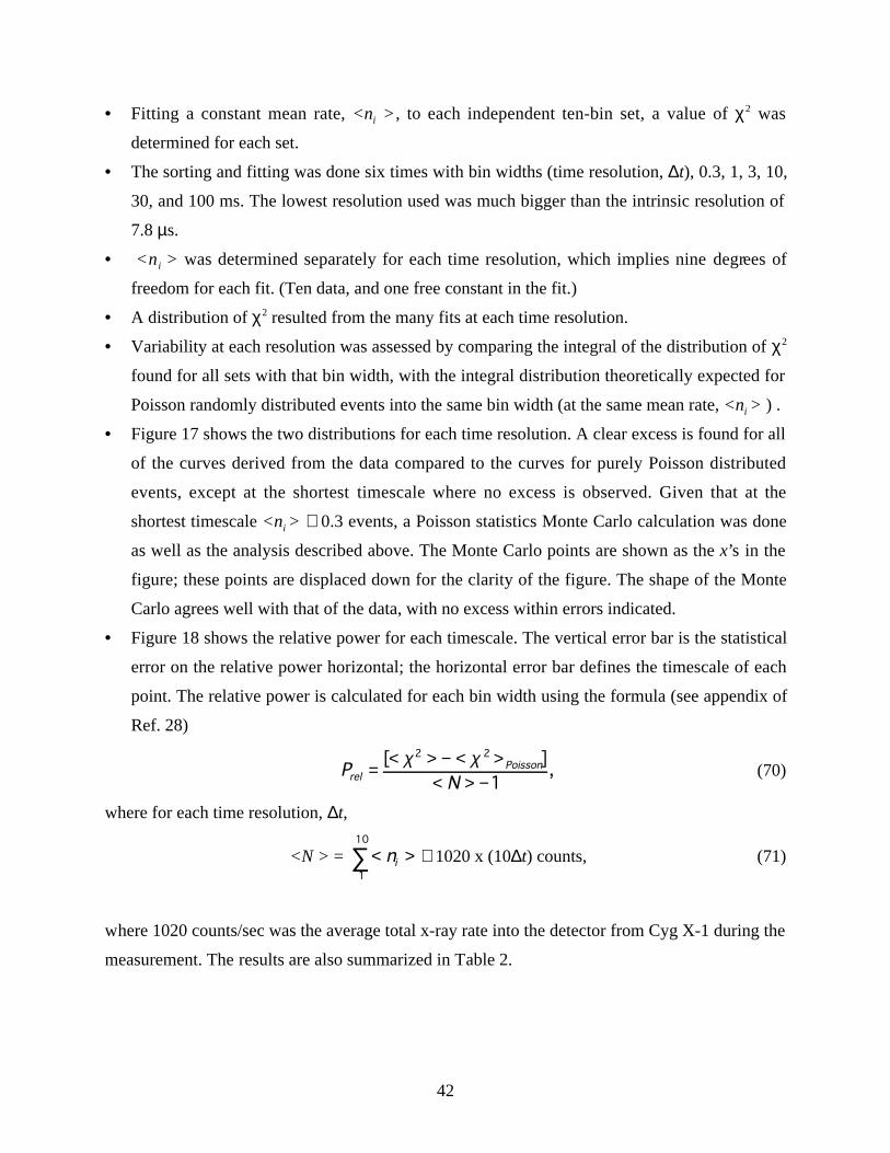
42
• Fitting a constant mean rate, <ni >, to each independent ten-bin set, a value of χ2 was
determined for each set.
• The sorting and fitting was done six times with bin widths (time resolution, ∆t), 0.3, 1, 3, 10,
30, and 100 ms. The lowest resolution used was much bigger than the intrinsic resolution of
7.8 µs.
• <ni > was determined separately for each time resolution, which implies nine degrees of
freedom for each fit. (Ten data, and one free constant in the fit.)
• A distribution of χ2 resulted from the many fits at each time resolution.
• Variability at each resolution was assessed by comparing the integral of the distribution of χ2
found for all sets with that bin width, with the integral distribution theoretically expected for
Poisson randomly distributed events into the same bin width (at the same mean rate, <ni > ) .
• Figure 17 shows the two distributions for each time resolution. A clear excess is found for all
of the curves derived from the data compared to the curves for purely Poisson distributed
events, except at the shortest timescale where no excess is observed. Given that at the
shortest timescale <ni > ≅ 0.3 events, a Poisson statistics Monte Carlo calculation was done
as well as the analysis described above. The Monte Carlo points are shown as the x’s in the
figure; these points are displaced down for the clarity of the figure. The shape of the Monte
Carlo agrees well with that of the data, with no excess within errors indicated.
• Figure 18 shows the relative power for each timescale. The vertical error bar is the statistical
error on the relative power horizontal; the horizontal error bar defines the timescale of each
point. The relative power is calculated for each bin width using the formula (see appendix of
Ref. 28)
PNrel
Poisson=< > − < >
< > −[ ]
,χ χ2 2
1(70)
where for each time resolution, ∆t,
<N > = < >∑ ni1
10
≅ 1020 x (10∆t) counts, (71)
where 1020 counts/sec was the average total x-ray rate into the detector from Cyg X-1 during the
measurement. The results are also summarized in Table 2.
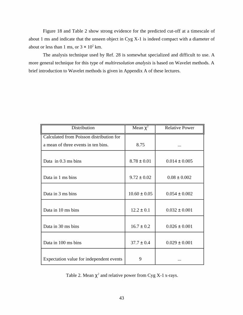
43
Figure 18 and Table 2 show strong evidence for the predicted cut-off at a timescale of
about 1 ms and indicate that the unseen object in Cyg X-1 is indeed compact with a diameter of
about or less than 1 ms, or 3 × 10² km.
The analysis technique used by Ref. 28 is somewhat specialized and difficult to use. A
more general technique for this type of multiresolution analysis is based on Wavelet methods. A
brief introduction to Wavelet methods is given in Appendix A of these lectures.
Distribution Mean χ2 Relative Power
Calculated from Poisson distribution for
a mean of three events in ten bins. 8.75 ...
Data in 0.3 ms bins 8.78 ± 0.01 0.014 ± 0.005
Data in 1 ms bins 9.72 ± 0.02 0.08 ± 0.002
Data in 3 ms bins 10.60 ± 0.05 0.054 ± 0.002
Data in 10 ms bins 12.2 ± 0.1 0.032 ± 0.001
Data in 30 ms bins 16.7 ± 0.2 0.026 ± 0.001
Data in 100 ms bins 37.7 ± 0.4 0.029 ± 0.001
Expectation value for independent events 9 ...
Table 2. Mean χ2 and relative power from Cyg X-1 x-rays.

44
45
4. X-Ray Astrophysics
This section focuses on the experimental and phenomenological aspects of x-ray astrophysics. X-
ray spectral and timing information can be useful in distinguishing the different types of x-ray
binary systems discussed above. Such information can be used in a general way as an adjunct to
the mass determination of the compact x-ray source to characterize neutron star vs. BHC
systems. In addition, detailed analysis of timing information, as discussed in Sec. 3e, can yield
quantitative information on the structure of these systems.
Figure 19 shows the HEAO A-1 x-ray all-sky map.29 The HEAO A-1 experiment was
described in Sec. 3e(i). The all-sky map shows about 1000 x-ray sources, many of which are
binary systems with a compact stellar object. The size of the dot is proportional to the log of the
intensity of the object. Sco X-1, a LMXB system containing an old neutron star, is by far the
brightest nontransient source in the sky. According to the HEAO A-1 catalogue, its intensity in
1–30 keV photons is 37.2 counts/sec/cm2.
Since x-rays from space are totally absorbed by the Earth’s atmosphere, experiments that
measure astronomical sources of x-rays must be done in space using satellite experiments.
Figure 20 shows a cartoon of the typical x-ray timing experiment in orbit. As contrasted with x-
ray imaging experiments, which have very fancy x-ray focusing optics and CCD detectors with
poor timing capability, timing experiments are very simple. (This includes the new generation of
timing experiments, USA and XTE discussed below, to be launched over the next couple of
years.) As the figure shows schematically for the USA experiment, they consist of an array of
multiwire proportional chambers (MWPC), two or more, shadowed by mechanical collimators
that limit the field of view to a few degrees or less. The satellite can be pointed at a source as is
the case in the figure or can be rotating in a survey mode. Past missions tended to spend
considerable time in survey mode, while the current generation of experiments will be pointed.
The intrinsic timing resolution of a multiwire proportional chamber is well within a µsec.
However, on-board data storage and telemetry bandwidth limitations have restricted past
experiments to operate, with minor exception (e.g., HEAO A-1), with ≥ 1 msec timing
resolution. Though the data collection deadtime from a single MWPC is about 20 µsec in the
new generation of instruments, an array of more than one MWPC allows effective inter-event
timing to 1 µsec. In addition, improvements in onboard data storage hardware and telemetry
rates allow the new generation of experiments to actually take advantage of the 1 µsec timing
46
resolution on a routine basis. Most of the data that comes down from USA and XTE will have <
few µsec timing resolution as well as some energy information for each γ event.
4a. X-Ray Discriminants of Black Holes vs. Neutron Stars
We start our discussion by considering the best studied BHC (BHC): Cyg X-1. This BHC is one
member of a binary star system that is extensively discussed in the literature.30 Cyg X-1 is a
binary star system with Right Ascension (RA) α = 19h 56m 28.9s, and Declination (Dec) δ =
35o 03′ 55″. The system is about 2.5 kpc (8.15 ly) distant from earth and is made of an unseen
compact object, its compactness determined from x-ray timing data as discussed in Sec. 3e(i),
and a visible stellar companion. The companion star, HDE 226868, is a ninth magnitude
supergiant B star that showed a simultaneous radio and x-ray intensity transition identifying it as
Cyg X-1’s companion. The x-ray source was the compact object and its accretion disk, while the
radio source was the B star. The system also shows a 5.6-day period as a spectroscopic binary
and the same period in soft x-ray variability.
Using the association of the B star, the current best estimate of the mass of the compact
object is Mx =16 ± 5 M§; this solution also yields 33 ± 9 M§ for the B star. This analysis was done
using the optical mass function, the spectral type of the B star, O-9.7 lab, the absence of eclipses,
and an estimate of the distance at 2.5 kpc from spectral reddening (interstellar dust). The analysis
also shows a strong limit of Mx > 7 M§. Optical photometry revealed ellipsoidal variations due to
tidal deformation of the B star that confirmed the orbital period and indicated a mass ratio
consistent with spectroscopic findings.
There is a concern with this analysis. In most HMXB systems, the visible star is found to
be undermassive by a factor of two to three for its temperature and luminosity. Some models
indicate that the primary in a black hole binary might be very undermassive. However, the best
mass determination for the B star companion for Cyg X-1 indicates that it has not lost (or
accreted) a large fraction of its mass during its evolution.
Even with the caveat above, Cyg X-1 is arguably the best stellar mass BHC that we know
of. With a lower limit on Mx of 7 M§, the compact object mass is well above the Rhoades and
Ruffini limit. This object has thus been carefully studied over the past 20 years in the x-ray to
characterize the x-ray emission of what many believe to be a black hole binary system. These
observations have led to a standard phenomenology of a BHC. Even though there may not be a
mass determination for a binary system, if it shows Cyg X-1 like x-ray behavior, it is labeled a
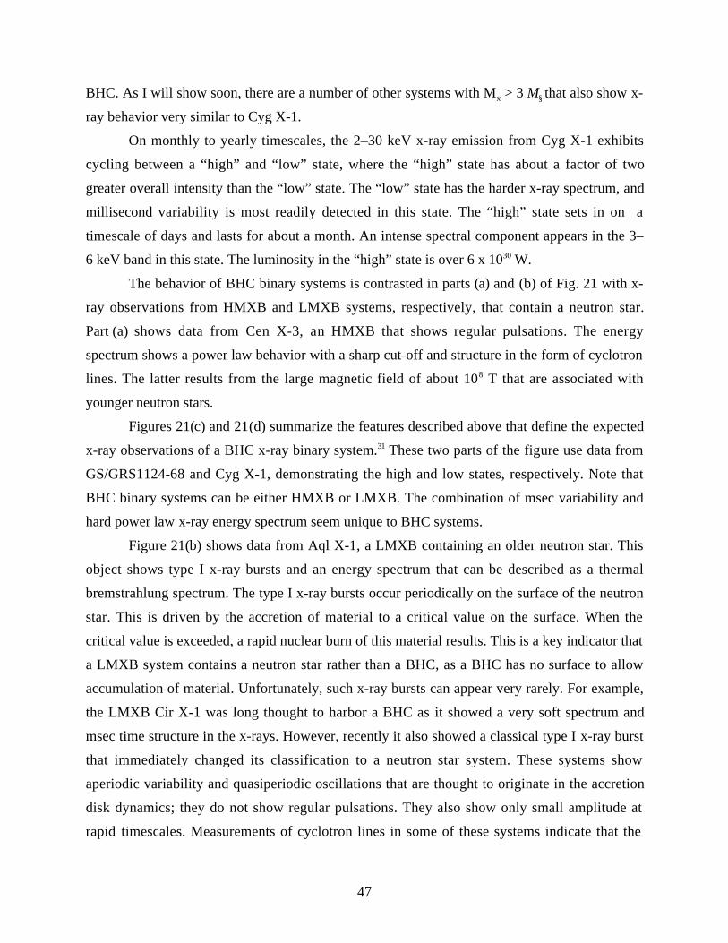
47
BHC. As I will show soon, there are a number of other systems with Mx > 3 M§ that also show x-
ray behavior very similar to Cyg X-1.
On monthly to yearly timescales, the 2–30 keV x-ray emission from Cyg X-1 exhibits
cycling between a “high” and “low” state, where the “high” state has about a factor of two
greater overall intensity than the “low” state. The “low” state has the harder x-ray spectrum, and
millisecond variability is most readily detected in this state. The “high” state sets in on a
timescale of days and lasts for about a month. An intense spectral component appears in the 3–
6 keV band in this state. The luminosity in the “high” state is over 6 x 1030 W.
The behavior of BHC binary systems is contrasted in parts (a) and (b) of Fig. 21 with x-
ray observations from HMXB and LMXB systems, respectively, that contain a neutron star.
Part (a) shows data from Cen X-3, an HMXB that shows regular pulsations. The energy
spectrum shows a power law behavior with a sharp cut-off and structure in the form of cyclotron
lines. The latter results from the large magnetic field of about 108 T that are associated with
younger neutron stars.
Figures 21(c) and 21(d) summarize the features described above that define the expected
x-ray observations of a BHC x-ray binary system.31 These two parts of the figure use data from
GS/GRS1124-68 and Cyg X-1, demonstrating the high and low states, respectively. Note that
BHC binary systems can be either HMXB or LMXB. The combination of msec variability and
hard power law x-ray energy spectrum seem unique to BHC systems.
Figure 21(b) shows data from Aql X-1, a LMXB containing an older neutron star. This
object shows type I x-ray bursts and an energy spectrum that can be described as a thermal
bremstrahlung spectrum. The type I x-ray bursts occur periodically on the surface of the neutron
star. This is driven by the accretion of material to a critical value on the surface. When the
critical value is exceeded, a rapid nuclear burn of this material results. This is a key indicator that
a LMXB system contains a neutron star rather than a BHC, as a BHC has no surface to allow
accumulation of material. Unfortunately, such x-ray bursts can appear very rarely. For example,
the LMXB Cir X-1 was long thought to harbor a BHC as it showed a very soft spectrum and
msec time structure in the x-rays. However, recently it also showed a classical type I x-ray burst
that immediately changed its classification to a neutron star system. These systems show
aperiodic variability and quasiperiodic oscillations that are thought to originate in the accretion
disk dynamics; they do not show regular pulsations. They also show only small amplitude at
rapid timescales. Measurements of cyclotron lines in some of these systems indicate that the
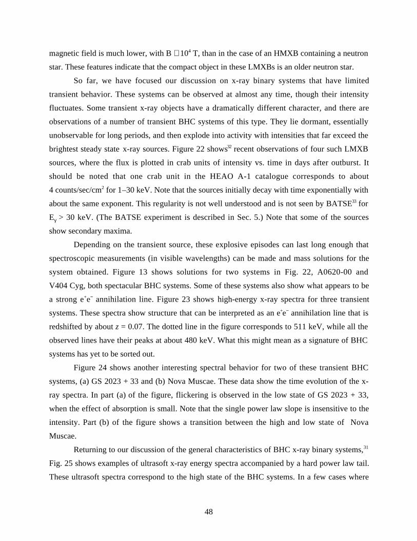
48
magnetic field is much lower, with B ≅ 104 T, than in the case of an HMXB containing a neutron
star. These features indicate that the compact object in these LMXBs is an older neutron star.
So far, we have focused our discussion on x-ray binary systems that have limited
transient behavior. These systems can be observed at almost any time, though their intensity
fluctuates. Some transient x-ray objects have a dramatically different character, and there are
observations of a number of transient BHC systems of this type. They lie dormant, essentially
unobservable for long periods, and then explode into activity with intensities that far exceed the
brightest steady state x-ray sources. Figure 22 shows32 recent observations of four such LMXB
sources, where the flux is plotted in crab units of intensity vs. time in days after outburst. It
should be noted that one crab unit in the HEAO A-1 catalogue corresponds to about
4 counts/sec/cm2 for 1–30 keV. Note that the sources initially decay with time exponentially with
about the same exponent. This regularity is not well understood and is not seen by BATSE33 for
Eγ > 30 keV. (The BATSE experiment is described in Sec. 5.) Note that some of the sources
show secondary maxima.
Depending on the transient source, these explosive episodes can last long enough that
spectroscopic measurements (in visible wavelengths) can be made and mass solutions for the
system obtained. Figure 13 shows solutions for two systems in Fig. 22, A0620-00 and
V404 Cyg, both spectacular BHC systems. Some of these systems also show what appears to be
a strong e+e− annihilation line. Figure 23 shows high-energy x-ray spectra for three transient
systems. These spectra show structure that can be interpreted as an e+e− annihilation line that is
redshifted by about z = 0.07. The dotted line in the figure corresponds to 511 keV, while all the
observed lines have their peaks at about 480 keV. What this might mean as a signature of BHC
systems has yet to be sorted out.
Figure 24 shows another interesting spectral behavior for two of these transient BHC
systems, (a) GS 2023 + 33 and (b) Nova Muscae. These data show the time evolution of the x-
ray spectra. In part (a) of the figure, flickering is observed in the low state of GS 2023 + 33,
when the effect of absorption is small. Note that the single power law slope is insensitive to the
intensity. Part (b) of the figure shows a transition between the high and low state of Nova
Muscae.
Returning to our discussion of the general characteristics of BHC x-ray binary systems,31
Fig. 25 shows examples of ultrasoft x-ray energy spectra accompanied by a hard power law tail.
These ultrasoft spectra correspond to the high state of the BHC systems. In a few cases where
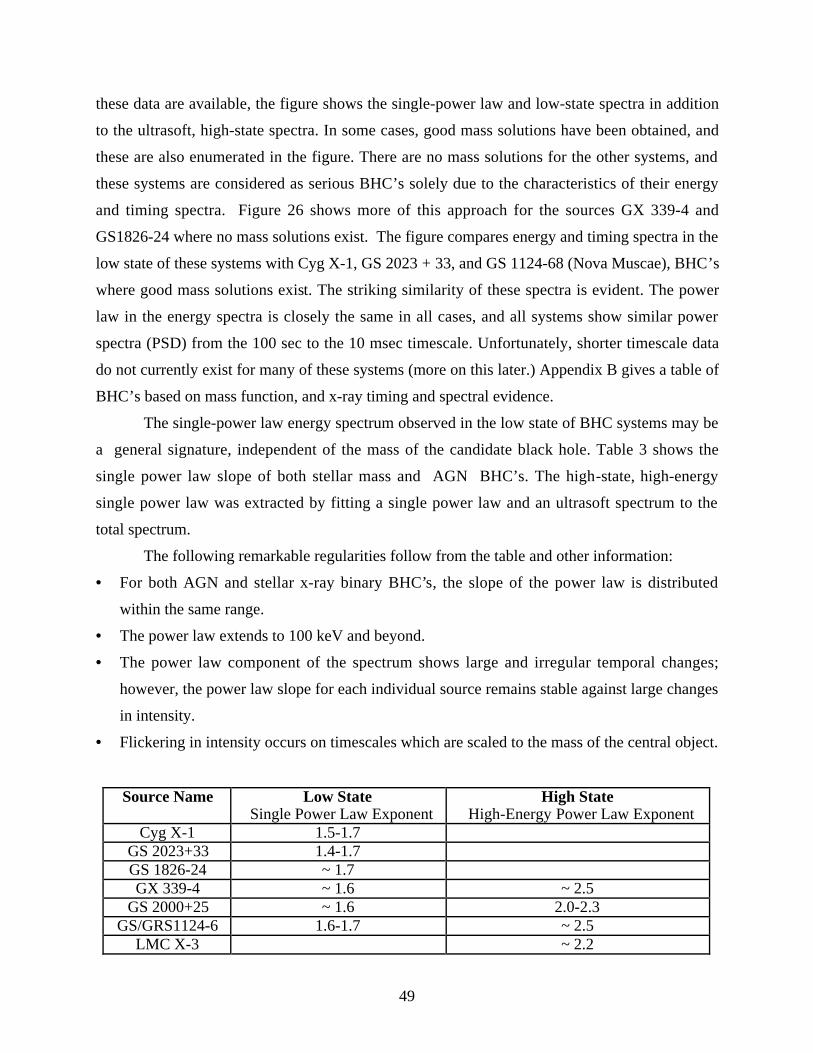
49
these data are available, the figure shows the single-power law and low-state spectra in addition
to the ultrasoft, high-state spectra. In some cases, good mass solutions have been obtained, and
these are also enumerated in the figure. There are no mass solutions for the other systems, and
these systems are considered as serious BHC’s solely due to the characteristics of their energy
and timing spectra. Figure 26 shows more of this approach for the sources GX 339-4 and
GS1826-24 where no mass solutions exist. The figure compares energy and timing spectra in the
low state of these systems with Cyg X-1, GS 2023 + 33, and GS 1124-68 (Nova Muscae), BHC’s
where good mass solutions exist. The striking similarity of these spectra is evident. The power
law in the energy spectra is closely the same in all cases, and all systems show similar power
spectra (PSD) from the 100 sec to the 10 msec timescale. Unfortunately, shorter timescale data
do not currently exist for many of these systems (more on this later.) Appendix B gives a table of
BHC’s based on mass function, and x-ray timing and spectral evidence.
The single-power law energy spectrum observed in the low state of BHC systems may be
a general signature, independent of the mass of the candidate black hole. Table 3 shows the
single power law slope of both stellar mass and AGN BHC’s. The high-state, high-energy
single power law was extracted by fitting a single power law and an ultrasoft spectrum to the
total spectrum.
The following remarkable regularities follow from the table and other information:
• For both AGN and stellar x-ray binary BHC’s, the slope of the power law is distributed
within the same range.
• The power law extends to 100 keV and beyond.
• The power law component of the spectrum shows large and irregular temporal changes;
however, the power law slope for each individual source remains stable against large changes
in intensity.
• Flickering in intensity occurs on timescales which are scaled to the mass of the central object.
Source Name Low State Single Power Law Exponent
High State High-Energy Power Law Exponent
Cyg X-1 1.5-1.7GS 2023+33 1.4-1.7GS 1826-24 ~ 1.7GX 339-4 ~ 1.6 ~ 2.5
GS 2000+25 ~ 1.6 2.0-2.3GS/GRS1124-6 1.6-1.7 ~ 2.5
LMC X-3 ~ 2.2
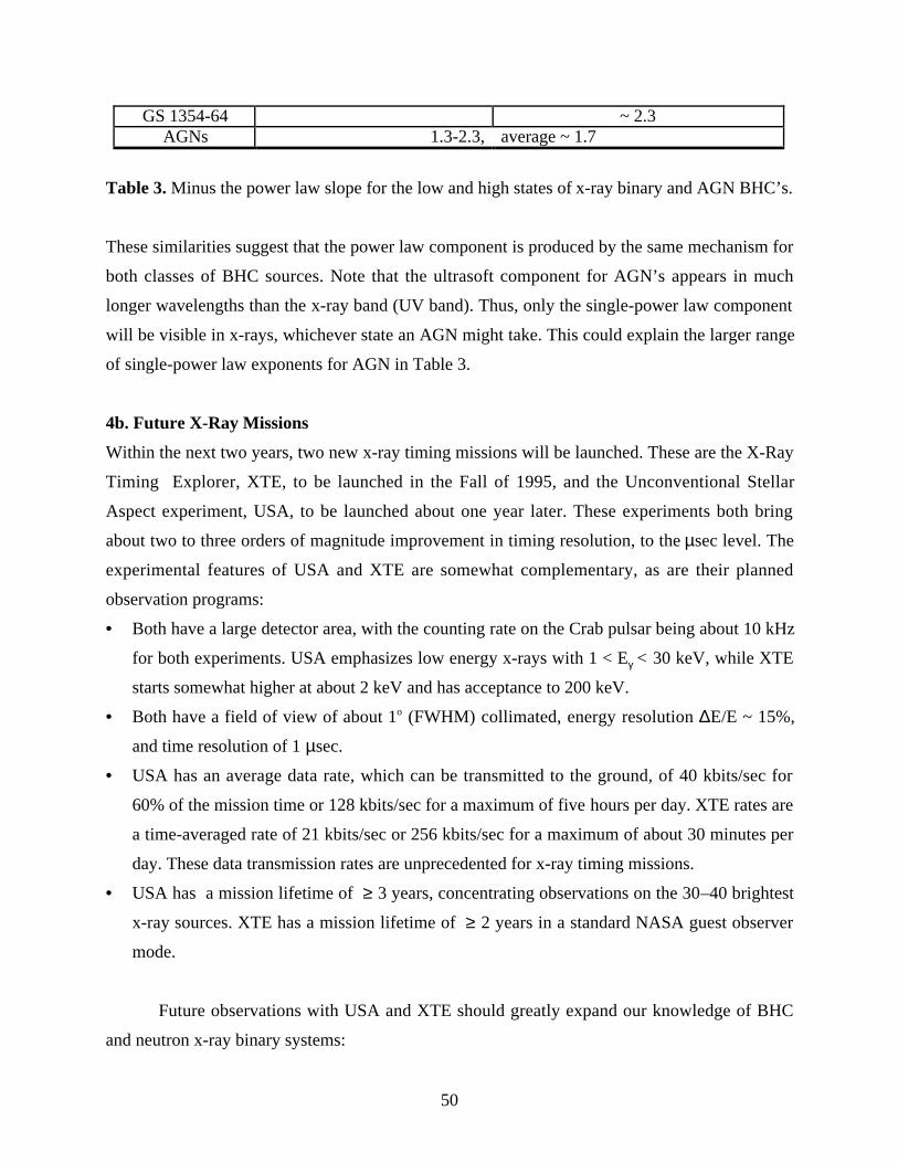
50
GS 1354-64 ~ 2.3AGNs 1.3-2.3, average ~ 1.7
Table 3. Minus the power law slope for the low and high states of x-ray binary and AGN BHC’s.
These similarities suggest that the power law component is produced by the same mechanism for
both classes of BHC sources. Note that the ultrasoft component for AGN’s appears in much
longer wavelengths than the x-ray band (UV band). Thus, only the single-power law component
will be visible in x-rays, whichever state an AGN might take. This could explain the larger range
of single-power law exponents for AGN in Table 3.
4b. Future X-Ray Missions
Within the next two years, two new x-ray timing missions will be launched. These are the X-Ray
Timing Explorer, XTE, to be launched in the Fall of 1995, and the Unconventional Stellar
Aspect experiment, USA, to be launched about one year later. These experiments both bring
about two to three orders of magnitude improvement in timing resolution, to the µsec level. The
experimental features of USA and XTE are somewhat complementary, as are their planned
observation programs:
• Both have a large detector area, with the counting rate on the Crab pulsar being about 10 kHz
for both experiments. USA emphasizes low energy x-rays with 1 < Eγ < 30 keV, while XTE
starts somewhat higher at about 2 keV and has acceptance to 200 keV.
• Both have a field of view of about 1o (FWHM) collimated, energy resolution ∆E/E ~ 15%,
and time resolution of 1 µsec.
• USA has an average data rate, which can be transmitted to the ground, of 40 kbits/sec for
60% of the mission time or 128 kbits/sec for a maximum of five hours per day. XTE rates are
a time-averaged rate of 21 kbits/sec or 256 kbits/sec for a maximum of about 30 minutes per
day. These data transmission rates are unprecedented for x-ray timing missions.
• USA has a mission lifetime of ≥ 3 years, concentrating observations on the 30–40 brightest
x-ray sources. XTE has a mission lifetime of ≥ 2 years in a standard NASA guest observer
mode.
Future observations with USA and XTE should greatly expand our knowledge of BHC
and neutron x-ray binary systems:
51
• USA will have weeks of µsec timing data at a rate of 128 kbit/sec on CYG-X-1 and other
BHC systems, as compared to minutes from HEAO A-1. XTE should also greatly expand the
µsec level timing data on these systems.
• Both experiments will have ≤ 4 µsec time resolution in this mode, corresponding to ≤ 1 km
spatial resolution (∆x ~ c∆t). They will also typically have energy information on each
photon, allowing a time-energy correlation to be made.
• A surface outside the horizon radius of a BHC may indicate a new state of matter. USA and
XTE have the timing resolution to see the power increase expected at these frequencies (∆t ~
2Rsurface /c), if such a surface exists. For true black holes, no power increase is expected for
frequencies higher than those produced in the accretion disk, and disk frequencies should be
cut off by the diameter of its inner edge (~ 6 Rsch).
More detailed information on each experiment is given in the following sections.
(i) The Unconventional Stellar Aspect Experiment––USA
Figure 27 shows an artist’s conception of the USA detector mounted on the rear of the ARGOS
satellite. USA is one of four scientific experiments on the satellite and has been in preparation
for about five years. The other three are ultraviolet experiments. ARGOS is scheduled to be
launched by the Air Force in the Fall of 1996. A full view of USA is depicted in the figure. The
inset shows John Hanson, Aero-Astro/SLAC graduate student, sitting in his creation––the
support structure and yoke for USA. Figure 28 gives an overview of the ARGOS satellite.
USA is a collaboration of the Naval Research Laboratory and Stanford University
(Physics Department and SLAC) scientists, with representation also from NASA-Ames,
Saddleback College, Sonoma State University, the University of Calgary, the University of
Oregon, and the University of Washington. It is designed to make long, pointed observations of
selected sources, with emphasis on lower x-ray energies than XTE. USA’s 1–30 keV energy
range extends that of XTE toward low energies where, for many sources, the counting rates are
considerably larger. The scientific goals of USA include many of the same as for XTE, but USA
will be used in an observation mode that dedicates large amounts of observing time (i.e., many
weeks of observing time over a three-year period) to each of 30–40 astronomical objects of
particular scientific interest to the collaboration. These measurements should engender a much
greater depth of understanding of these BHC and neutron star accretion systems compared to
52
current measurements. USA’s observing mode is scientifically complementary to the planned
functioning of XTE as a general purpose x-ray timing observatory, to be used by guest
investigators in a great variety of observing programs, each of short duration. For more details
about USA, see the World Wide Web at URL:
http:\\www.slac.stanford.edu\group_k
or contact the USA Principal Investigator Kent Wood, or SLAC Co-Investigator Elliott Bloom at
these respective Internet addresses: [email protected], and [email protected].
The USA x-ray detector system consists of two multiwire proportional chambers, side by
side, shadowed by copper hexel collimators that define a 1.2o cone on the sky (FWHM). The
chambers are filled with P10 gas at 1.1 ATM, with enough gas stored for a three-to-six year
lifetime. A unique feature of this chamber is a 2.5 µm mylar window. Such very thin windows
have been flown successfully by the NRL x-ray group in a number of past missions. This
window, together with the 2.5 µm aluminized mylar heat shield, is thin enough to allow
measurement of x-rays down to 1 keV. The energy acceptance of the detector is 1–30 keV. The
effective aperture of both chambers through the collimators is 2000 cm2 at 3 keV. The system
has an energy resolution of ∆E/E = 17% , which is about 1 keV at 5.9 keV. In order to reject
charge particle backgrounds, the chamber has a built-in anticoincidence system. This five-sided
cosmic-ray veto gives a residual rate of 4 × 10⁻³ counts/cm2/sec at 1–10 keV.
The USA experiment is unique among all x-ray experiments, including XTE, in that it is
integrated with a GPS receiver on board the ARGOS spacecraft. This will allow absolute timing
to the microsecond level over long periods of time. The GPS timing signal combined with the
µsec capability of the USA experiment will result in unprecedented microsecond timing
information for an x-ray experiment.
(ii) The X-Ray Timing Explorer––XTE33
Figure 29 shows a schematic of the XTE. This satellite contains three experiments that are
dedicated to x-ray timing and has been in preparation by NASA for about 15 years. The three
instruments on the observatory are the proportional counter array, PCA, the high-energy x-ray
timing experiment, HEXTE, and the all-sky monitor, ASM. XTE is due to be launched into low
earth orbit in late 1995. The instruments on XTE are a collaboration of the NASA Goddard
53
Space Flight Center, Massachusetts Institute of Technology, and the University of California at
San Diego. It will make pointed observations with both the PCA and HEXTE, and scanning
observations with the smaller ASM. The pointed observations will be selected by NASA peer
review from proposals submitted in response to a NASA Research Announcement.
XTE will have the following scheduling features for scientific reasons. Sources more
than 30o off the ecliptic can be observed at any time. Time-constrained observations will be
supported, e.g., in order to observe objects at specific epochs, to allow participation in
collaborative multiwavelength observations, and for repeated observations. There will be
provisions to monitor given sets of objects, such as AGN, or x-ray binaries, with short
observations. Transients will be observable with the pointed detectors within seven hours of
detection by the ASM or notification from another observatory.
The studies to be carried out by XTE include the nature of black holes (including those
that may be in AGN), neutron stars, and white dwarfs––their interactions with their environs, the
systems in which they are formed, and their ultimate fates. The objectives will include, where
appropriate, the interior composition and properties, and relationships between magnetic and
rotation axes. Of special interest are radiation generation mechanisms, disk and wind
instabilities, x-ray transients, the end points of binary system evolution, and the formation of the
x-ray background due to cosmologically distributed AGN. For more details about XTE, see the
World Wide Web at this URL:
http://heasarc.gsfc.nasa.gov/0/docs/xte/xte.html
or contact the Principal Investigator Jean Swank at this Internet address:
The PCA and HEXTE are designed to take pointed observations. The PCA measures x-
rays in the 2–60 keV region and has an exceptionally large effective collecting area of 6250 cm2.
The energy resolution is 18% at 6 keV. It consists of five separate gas-filled multiwire
proportional chambers, each with a collimator and a sun shade. The detectors are sealed with
Xenon gas which gives them acceptance to 60 keV. The background is kept very low by means
of anticoincidence chambers on four sides of the detection chamber. The HEXTE system is
54
sensitive to 20–200 keV x-rays. There are two “rocking” clusters, each with 4 NaI/CsI
“phoswich” detectors. A single phoswich detector consists of a 3 mm thick NaI primary detector
coupled to a 38 mm thick CsI anticoincidence crystal that also serves as a light guide to the
photomultiplier tube. These lie inside a five-sided plastic scintillator anticoincidence shield. Each
detector has 200 cm2 net effective area. Each cluster contains four detectors; the total net area of
the entire system is 1600 cm2. The field of view is 1o FWHM and is coaligned with the PCA.
The third XTE instrument is the ASM. This device scans 80% of the sky every ~100
minutes to monitor the intensity of the brightest ~ 75 x-ray sources and to provide an alert if a
source changes state or brightens suddenly. This allows the spacecraft to be maneuvered so the
PCA/HEXTE systems can study the event. The ASM consists of three scanning shadow cameras
on one rotating boom with a total effective area of 90 cm2. Each device is a “Dicke camera”
consisting of a one-dimensional mask and a one-dimensional position-sensitive proportional
counter. The gross field of view of a single camera is 6o × 90o FWHM, and the angular
resolution in the imaging direction is 0.2o. The intensities and other basic results derived from the
ASM data will immediately be made available in the XTE science operations center and to the
community in general via computer links. With its combination of instruments and broad user
community, XTE should bring rapid progress to many subfields of x-ray timing astronomy and
astrophysics (and particle astrophysics).
In summary, Fig. 30 shows the effective x-ray acceptance vs. energy of past, current, and
future x-ray satellite detectors for 1–200 keV. The acceptance of USA is shown as dots, while
the XTE PCA is the top solid line in the figure. The XTE HEXTE effective acceptance, taking
into account routine off-target background scans, is shown as the top dashed line starting at about
20 keV. XTE will make a dramatic increase in effective area compared to past experiments over
much of the energy range shown. USA will have an increased effective area below 2 keV,
compared to past timing experiments, due to its ultrathin mylar window.
5. Gamma-Ray Astrophysics
With the launch of the Compton Gamma-Ray Observatory (CGRO) by NASA in early 1991, a
dramatic influx of new gamma-ray data in the 0.5 MeV–30 GeV energy range became available
to investigators. The CGRO34 consists of four experiments. The Burst and Transient Source
Experiment (BATSE) studies short-lived phenomena, such as gamma-ray bursts. The Oriented
Scintillation Spectrometer Experiment (OSSE) measures the low-energy gamma-ray spectrum of
55
celestial objects, in particular, higher energy x-ray and lower energy gamma-ray lines from
atoms and nuclei. The Imaging Compton Telescope (COMPTEL) measures gamma-rays in the
MeV to tens of MeV range, with an emphasis on higher energy nuclear lines. Finally, the
Energetic Gamma-Ray Experiment Telescope (EGRET) is the highest energy gamma-ray
instrument measuring γ's in the 50 MeV–30 GeV range. In this section, we will concentrate on
the results of BATSE and EGRET. Both of these instruments have made contributions that are of
considerable interest to particle physics.
5a. Gamma-Ray Bursters
Gamma-ray bursts are intense transient bursts of γ’s with spectral contribution from the x-ray
region to about 20 GeV (the highest energy burst photon yet observed by the EGRET
experiment).35 These bursts have a complicated temporal structure and have been observed to
have durations from less than 0.1 sec to more than 500 sec. They were first discovered by the
American, classified, VELA satellites that were placed in orbit to detect clandestine nuclear
explosions above the surface of the earth. The startling discovery of naturally occurring gamma-
ray bursts over the celestial sphere took a number of years to be made public due to classification
issues.
Figure 31, adapted from G. Fishman,36 indicates that the development of theories of
gamma-ray bursts is based upon relatively little data which, in turn, have been controversial.
BATSE has broadened the observational base considerably over the past four years with much
reliable data. This data flow should continue for the life of the CGRO satellite. Indeed, pre-
BATSE, over 100 theoretical papers were published speculating on the nature of these
phenomena. Since BATSE has begun, more than 50 additional theoretical papers have addressed
this issue.37 In the past, the theories, in the large, were concerned with neutron star models of
gamma-ray bursts. However, the uniformity of these bursts on the sky, which we shall discuss in
some detail, has made it very difficult for the neutron star source models. This is because neutron
stars are thought to be a product of the death of stars that are congregated in the plane of the
galaxy. Thus, one would expect to see the influence of the galactic plane in the distribution of
bursters on the sky. None is observed by BATSE, which has placed new emphasis on
cosmological models of gamma-ray bursts.

56
• The pre-BATSE theoretical near consensus that bursts were galactic, originating from a
neutron star population having a strong magnetic field, was based on the following
observational information:
• Millisecond fluctuations in the burst intensity indicated a compact object consistent with a
neutron star.
• Observation of spectral lines in the 20 keV–66 keV range by the GINGA satellite38 are
interpreted as cyclotron lines corresponding to a 108 T magnetic field, which is consistent
with a neutron star. (To this date, OSSE has not confirmed these observations.)
• There are no quiescent counterpart sources to bursts that have been observed. This is
compatible with the burst source being an isolated compact object.
• In some bursts, soft x-ray tails can be fit by a blackbody spectra with T ≈ 3 keV. This implies
through model calculations a source radius, R = 0.7 (d/1 kpc) km. Such a source structure is
consistent with the polar region of a neutron star for bursters with d < 10 kpc, i.e., galactic
sources.
These pre-BATSE (and OSSE) experimental results led to many, many models for
bursters based on a galactic population of isolated neutron stars. One unavoidable prediction
from these models was that detectors of increased sensitivity should see an anisotropy in the
burster distribution on the sky towards the galactic plane. BATSE, which has now collected well
over 1500 bursts, has not observed this predicted anisotropy to levels that make galactic models
of bursters highly unlikely.
BATSE39 consists of eight identically configured detector modules and a Central
Electronics Unit (CEU). Each detector module contains two NaI(Tl) scintillation detectors: a
Large Area Detector (LAD) optimized for sensitivity and directional response, and a
Spectroscopy Detector (SD) optimized for energy coverage and energy resolution. The eight
planes of the LADs are parallel to the eight faces of a regular octahedron, with the orthogonal
primary axes of the octahedron aligned with the coordinate axes of the CGRO spacecraft. The
detectors are mounted to the eight corners of the spacecraft.
The LAD detector is a disk of NaI scintillation crystal 20 inches in diameter and 0.5-inch
thick, mounted on a 0.75-inch layer of quartz. The large diameter-to-thickness ratio of the
scintillation crystal produces a detector response similar to that of a cosine function at low
57
energies where the crystal is opaque to incident radiation. At energies above 300 keV, the
angular response is flatter than a cosine. A light collector housing on each detector brings the
scintillation light into three five-inch-diameter photomultiplier tubes. The signals from the three
tubes are summed at the detector. A 0.25-inch plastic scintillation detector in front of the LAD is
used as an anticoincidence shield to reduce the background due to charged particles. A thin lead
and tin shield inside the light collector housing reduces the amount of background and scattered
radiation entering the back side.
The spectroscopy detector is an uncollimated NaI(Tl) scintillation detector five inches in
diameter and three inches thick. A single five-inch photomultiplier tube is directly coupled to
the scintillation detector window. The housing of the PMT has a passive lead/tin shield similar to
that of the LADs. The crystal housing has a three-inch-diameter, 50 mm thick beryllium window
on its front face in order to provide high efficiency down to 10 keV. The axis of symmetry of an
SD is offset by 19o from the LAD axis for mechanical reasons.
Scintillation pulses from the detectors are processed by a gated baseline restoration
circuit in order to minimize spectral distortion at high counting rates. Pulses are processed in
parallel by a high-speed, four-channel discriminator circuit and by a slower, pulse-height
analyzer system. The nominal equivalent energies of the upper three discriminators for the
LADs are 60, 110, and 325 keV. The lower-level discriminators are programmable and currently
set near 20 keV. Two of the fast discriminators for the SD’s are set at energies above the
energies analyzed by the pulse height system. The gain of each detector system is determined by
the high voltage applied to the PMT’s. The SD’s are operated at three different gains in order to
span from 10 keV to greater than 100 MeV.
Each of the eight BATSE detector modules sends data to the Central Electronics Unit
(CEU). The CEU contains hardware and software that accumulates the data into several large
RAM memory buffers. Extensive use of commandable parameters, plus the capability to
reprogram the flight software, ensures that BATSE has the flexibility to respond to unforeseen
conditions or newly discovered gamma-ray phenomena. Signals from the pulse-height
converters are used to construct 128-channel spectra from the LAD’s and 256-channel spectra
from the SD’s. Each of the spectra are subdivided into ranges with different dispersions to
increase the dynamic range and to efficiently use the available telemetry space. These energy
channels are also mapped into 16 coarse energy channels using programmable look-up tables,
one for the LAD’s and one for the SD’s. This permits the trade of time resolution for energy
58
resolution in several of the data types. Discriminator events are accumulated in the hardware
every 64 ms. The CEU hardware constructs various data types from the discriminator counts,
and the 16-channel, 128-channel, and 256-channel count spectra.
BATSE detects gamma-ray bursts on-board by examining the count rates of each of the
eight LAD’s for statistically significant increases above background on each of the three
timescales: 64 ms, 256 ms, and 1024 ms. The discriminator rates in channels 2 and 3
(approximately 55–325 keV) are used. The background rate is determined for each detector over
a commandable time interval currently set at 17.4 seconds. The statistical significance required
for a burst trigger is set separately for each of the three timescales, with a quantization of
0.0625 sigma. These thresholds are currently set at 5.5 sigma. At least two detectors must
exceed threshold for a burst trigger to occur. An additional requirement for burst triggering is
that the detector with the greatest increase in count rate must have an increase in the charged
particle rate that is less than a specified fraction of the increase in the neutral rate. This is done
in order to avoid triggering on charged-particle event encounters, such as those produced by
spacecraft containing nuclear reactor power sources.
When a gamma-ray burst is detected, the CEU enters a fast data acquisition mode and
rapidly stores a variety of data types into memory. Over the period of a CGRO orbit, the
normally scheduled output of pulsar and high resolution spectra is suspended, and the collected
burst data is read out in the variable portion of the data packets. The normal output schedule
then resumes, in proper synchronization with the CGRO orbit. While the burst memories are
being telemetered, the trigger thresholds are temporarily revised to values corresponding to the
maximum rates detected during the burst. Thus, a stronger burst will terminate the readout of a
weaker burst and overwrite the burst memories. The data available from an overwritten burst is
timing dependent but includes, at a minimum, the 64-ms-resolution discriminator data
(DISCSC).
The error in angular location40 of burst events is the radius of a circle having the same
area as the 68% confidence ellipse defined by the formal covariance matrix from a minimum χ2
fit on the assumption of normal errors. The error is based solely on the Poisson uncertainty in
the BATSE measurement of burst flux by each LAD. There is, in addition, an RMS systematic
error of approximately four degrees. Adding four degrees in quadrature to the error from the fit
yields an estimate of the 68% confidence interval for the burst location error. One does not
expect a normal distribution of errors, particularly when a burst is weak (and the error in the
59
basic measurement is large). The 95% confidence interval may be three to four times the size of
the 68% confidence interval.
Figure 32 shows the duration distribution for 222 BATSE bursts41 as measured by T90,
where T90 is the time interval during which the integrated counts go from 5% to 95% of the total
integrated counts in the burst. The solid histogram is the raw data, while the dashed histogram,
essentially the same as the solid histogram, is the raw data convolved with measurement errors.
The data seem to show a bimodal distribution with one “peak” at about 0.3 sec and the other at
about 35 secs.
Figure 33 shows some “typical” burst profiles of counts per second vs. time during the
burst; these are called light curves. Two distinct types of bursts appear in the figure. Parts (a)–(d)
show four typical multipeaked complex light curves, while (e)–(h) show four typical smooth
light curves. For all parts of the figure, the energy range of photons in the light curve is 50–
300 keV.
Figure 34 shows the distribution of the energy of the peak emission per unit logarithmic
energy interval for a number of bursts. As the figure shows, there are some bursts that have peak
emission in the 1 MeV range. Energy spectra of a burst can also be characterized by an effective
power law index, α, i.e., Eα. Figure 35 shows a distribution of the effective power law index for a
sample of 222 BATSE bursts measured over the energy range 50–300 keV. The solid line
represents the distribution for the peak rate spectrum, and the dotted line represents the
distribution for the total fluence spectrum. The effective power law peaks at α ≈ −1.7, but has a
broad distribution which extends to values greater than zero for this energy range.
Of course, the most exciting result to date from the BATSE experiment is the
observation of an isotropic distribution of bursts on the celestial sphere.42 Figure 36 shows the
BATSE burst distribution in galactic coordinates for the first 743 events. As previously discussed
in detail, the direction to each burst is determined using the relative count rate on the eight
LAD’s, one at each corner of the CGRO spacecraft. The error on the location, σθ, is about 13o
statistical and 4o systematic. Table 4 lists the values of the statistics for the ensemble of 743
bursts.
Six statistics are used to measure the anisotropy. Two galactic statistics test most
sensitively for galactic patterns, and thus, are best for testing the question of galactic vs.
cosmological origin. The statistic <cosθ >, where θ is the angle between the burst and the
galactic center, tests for a concentration towards the galactic center, while the statistic <sin2b-
60
1/3>, where b is the galactic latitude, tests for a concentration in the galactic plane. Two
coordinate-system independent statistics43 test for significant dipole and quadrupole moments in
a model-independent way. The Rayleigh-Watson statistic, W, tests the size of the dipole moment,
while the Bingham statistic, B, measures the deviation of the quadrupole moments from the
values expected for isotropy. Finally, two equatorial-based statistics test for the artificial
anisotropy caused by the proximity of the Earth to the spacecraft. The statistic <sin2δ - 1/3>,
where δ is the declination to the burst, is sensitive to the quadrupole moment caused by the
reduced exposure of the equatorial region, and the statistic < sinδ > is sensitive to the dipole
moment towards the North Pole caused by turning the instrument off in the South Atlantic
Anomaly.
The direction of a burst is measured by the relative counting rate from each of the eight
LAD’s during the burst. The error listed in the fourth and fifth columns of Table 4 are the 1σ
finite sample fluctuation. This comparison between the next-to-last and the last columns
indicates the evidence for isotropy. No evidence for anisotropy is seen in the table. The
distribution of bursts is consistent with an isotropic distribution on the sky. The errors are small
enough that galactic halo models are also limited. For the extended (neutron star) halo model, the
data requires most burst sources to be at least 100 kpc from the galactic center, regardless of the
freedom to adjust the form of the radial distribution. In addition, there are essentially no repeater
bursts; that is, each source has been seen only once. If these bursts are cosmological in origin,
there must be an enormous power in the burst, much greater than typical bursts associated with
neutron stars. Such power could arise from the merging of two neutron stars into a black hole. It
seems like we have a real mystery on our hands.
5b. Results from High-Energy Gamma-Ray Experiments
High-energy gamma-ray astronomy is a relatively young science with the first experiments being
done from space in about 1962, and the first ground-based ultra high-energy experiments
(> 0.5 TeV) starting up in the mid-1970s. Table 5 shows a list of orbiting high-energy gamma-
ray telescope missions to date and the increasing sensitivity as time has progressed.
Instrument Year of Launch Photons DetectedEXP XI 1962 31OSO-3 1968 621SAS-2 1972 8,000
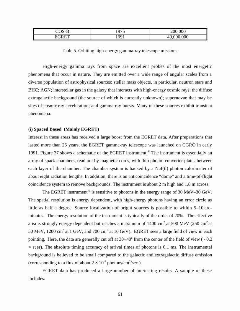
61
COS-B 1975 200,000EGRET 1991 40,000,000
Table 5. Orbiting high-energy gamma-ray telescope missions.
High-energy gamma rays from space are excellent probes of the most energetic
phenomena that occur in nature. They are emitted over a wide range of angular scales from a
diverse population of astrophysical sources: stellar mass objects, in particular, neutron stars and
BHC; AGN; interstellar gas in the galaxy that interacts with high-energy cosmic rays; the diffuse
extragalactic background (the source of which is currently unknown); supernovae that may be
sites of cosmic-ray acceleration; and gamma-ray bursts. Many of these sources exhibit transient
phenomena.
(i) Spaced Based (Mainly EGRET)
Interest in these areas has received a large boost from the EGRET data. After preparations that
lasted more than 25 years, the EGRET gamma-ray telescope was launched on CGRO in early
1991. Figure 37 shows a schematic of the EGRET instrument.44 The instrument is essentially an
array of spark chambers, read out by magnetic cores, with thin photon converter plates between
each layer of the chamber. The chamber system is backed by a NaI(tl) photon calorimeter of
about eight radiation lengths. In addition, there is an anticoincidence “dome” and a time-of-flight
coincidence system to remove backgrounds. The instrument is about 2 m high and 1.8 m across.
The EGRET instrument45 is sensitive to photons in the energy range of 30 MeV–30 GeV.
The spatial resolution is energy dependent, with high-energy photons having an error circle as
little as half a degree. Source localization of bright sources is possible to within 5–10 arc-
minutes. The energy resolution of the instrument is typically of the order of 20%. The effective
area is strongly energy dependent but reaches a maximum of 1400 cm2 at 500 MeV (250 cm2 at
50 MeV, 1200 cm2 at 1 GeV, and 700 cm2 at 10 GeV). EGRET sees a large field of view in each
pointing. Here, the data are generally cut off at 30–40o from the center of the field of view (~ 0.2
× π sr). The absolute timing accuracy of arrival times of photons is 0.1 ms. The instrumental
background is believed to be small compared to the galactic and extragalactic diffuse emission
(corresponding to a flux of about 2 × 10⁻⁵ photons/cm2/sec.).
EGRET data has produced a large number of interesting results. A sample of these
includes:
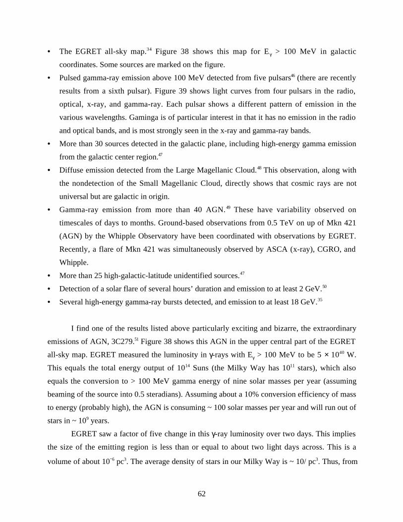
62
• The EGRET all-sky map.34 Figure 38 shows this map for E γ > 100 MeV in galactic
coordinates. Some sources are marked on the figure.
• Pulsed gamma-ray emission above 100 MeV detected from five pulsars46 (there are recently
results from a sixth pulsar). Figure 39 shows light curves from four pulsars in the radio,
optical, x-ray, and gamma-ray. Each pulsar shows a different pattern of emission in the
various wavelengths. Gaminga is of particular interest in that it has no emission in the radio
and optical bands, and is most strongly seen in the x-ray and gamma-ray bands.
• More than 30 sources detected in the galactic plane, including high-energy gamma emission
from the galactic center region.47
• Diffuse emission detected from the Large Magellanic Cloud.48 This observation, along with
the nondetection of the Small Magellanic Cloud, directly shows that cosmic rays are not
universal but are galactic in origin.
• Gamma-ray emission from more than 40 AGN.49 These have variability observed on
timescales of days to months. Ground-based observations from 0.5 TeV on up of Mkn 421
(AGN) by the Whipple Observatory have been coordinated with observations by EGRET.
Recently, a flare of Mkn 421 was simultaneously observed by ASCA (x-ray), CGRO, and
Whipple.
• More than 25 high-galactic-latitude unidentified sources.47
• Detection of a solar flare of several hours’ duration and emission to at least 2 GeV.50
• Several high-energy gamma-ray bursts detected, and emission to at least 18 GeV.35
I find one of the results listed above particularly exciting and bizarre, the extraordinary
emissions of AGN, 3C279.51 Figure 38 shows this AGN in the upper central part of the EGRET
all-sky map. EGRET measured the luminosity in γ-rays with Eγ > 100 MeV to be 5 × 1040 W.
This equals the total energy output of 1014 Suns (the Milky Way has 1011 stars), which also
equals the conversion to > 100 MeV gamma energy of nine solar masses per year (assuming
beaming of the source into 0.5 steradians). Assuming about a 10% conversion efficiency of mass
to energy (probably high), the AGN is consuming ~ 100 solar masses per year and will run out of
stars in ~ 109 years.
EGRET saw a factor of five change in this γ-ray luminosity over two days. This implies
the size of the emitting region is less than or equal to about two light days across. This is a
volume of about 10-6 pc3. The average density of stars in our Milky Way is ~ 10/ pc3. Thus, from
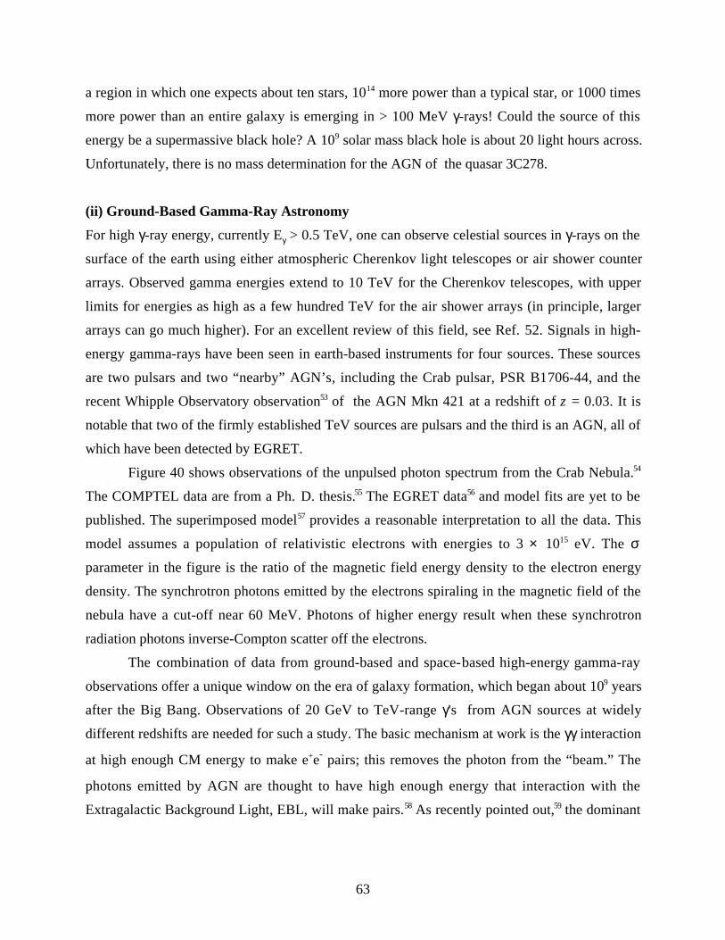
63
a region in which one expects about ten stars, 1014 more power than a typical star, or 1000 times
more power than an entire galaxy is emerging in > 100 MeV γ-rays! Could the source of this
energy be a supermassive black hole? A 109 solar mass black hole is about 20 light hours across.
Unfortunately, there is no mass determination for the AGN of the quasar 3C278.
(ii) Ground-Based Gamma-Ray Astronomy
For high γ-ray energy, currently Eγ > 0.5 TeV, one can observe celestial sources in γ-rays on the
surface of the earth using either atmospheric Cherenkov light telescopes or air shower counter
arrays. Observed gamma energies extend to 10 TeV for the Cherenkov telescopes, with upper
limits for energies as high as a few hundred TeV for the air shower arrays (in principle, larger
arrays can go much higher). For an excellent review of this field, see Ref. 52. Signals in high-
energy gamma-rays have been seen in earth-based instruments for four sources. These sources
are two pulsars and two “nearby” AGN’s, including the Crab pulsar, PSR B1706-44, and the
recent Whipple Observatory observation53 of the AGN Mkn 421 at a redshift of z = 0.03. It is
notable that two of the firmly established TeV sources are pulsars and the third is an AGN, all of
which have been detected by EGRET.
Figure 40 shows observations of the unpulsed photon spectrum from the Crab Nebula.54
The COMPTEL data are from a Ph. D. thesis.55 The EGRET data56 and model fits are yet to be
published. The superimposed model57 provides a reasonable interpretation to all the data. This
model assumes a population of relativistic electrons with energies to 3 × 10¹⁵ eV. The σ
parameter in the figure is the ratio of the magnetic field energy density to the electron energy
density. The synchrotron photons emitted by the electrons spiraling in the magnetic field of the
nebula have a cut-off near 60 MeV. Photons of higher energy result when these synchrotron
radiation photons inverse-Compton scatter off the electrons.
The combination of data from ground-based and space-based high-energy gamma-ray
observations offer a unique window on the era of galaxy formation, which began about 109 years
after the Big Bang. Observations of 20 GeV to TeV-range γ's from AGN sources at widely
different redshifts are needed for such a study. The basic mechanism at work is the γγ interaction
at high enough CM energy to make e+e- pairs; this removes the photon from the “beam.” The
photons emitted by AGN are thought to have high enough energy that interaction with the
Extragalactic Background Light, EBL, will make pairs.58 As recently pointed out,59 the dominant
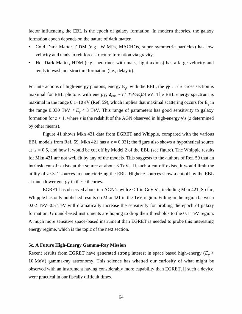
64
factor influencing the EBL is the epoch of galaxy formation. In modern theories, the galaxy
formation epoch depends on the nature of dark matter.
• Cold Dark Matter, CDM (e.g., WIMPs, MACHOs, super symmetric particles) has low
velocity and tends to reinforce structure formation via gravity.
• Hot Dark Matter, HDM (e.g., neutrinos with mass, light axions) has a large velocity and
tends to wash out structure formation (i.e., delay it).
For interactions of high-energy photons, energy Eγ, with the EBL, the γγ→ e+e− cross section is
maximal for EBL photons with energy, εEBL ~ (1 TeV/Eγ)/3 eV. The EBL energy spectrum is
maximal in the range 0.1–10 eV (Ref. 59), which implies that maximal scattering occurs for Eγ in
the range 0.030 TeV < Eγ < 3 TeV. This range of parameters has good sensitivity to galaxy
formation for z < 1, where z is the redshift of the AGN observed in high-energy γ’s (z determined
by other means).
Figure 41 shows Mkn 421 data from EGRET and Whipple, compared with the various
EBL models from Ref. 59. Mkn 421 has a z = 0.031; the figure also shows a hypothetical source
at z = 0.5, and how it would be cut off by Model 2 of the EBL (see figure). The Whipple results
for Mkn 421 are not well-fit by any of the models. This suggests to the authors of Ref. 59 that an
intrinsic cut-off exists at the source at about 3 TeV. If such a cut off exists, it would limit the
utility of z << 1 sources in characterizing the EBL. Higher z sources show a cut-off by the EBL
at much lower energy in these theories.
EGRET has observed about ten AGN’s with z < 1 in GeV γ's, including Mkn 421. So far,
Whipple has only published results on Mkn 421 in the TeV region. Filling in the region between
0.02 TeV–0.5 TeV will dramatically increase the sensitivity for probing the epoch of galaxy
formation. Ground-based instruments are hoping to drop their thresholds to the 0.1 TeV region.
A much more sensitive space-based instrument than EGRET is needed to probe this interesting
energy regime, which is the topic of the next section.
5c. A Future High-Energy Gamma-Ray Mission
Recent results from EGRET have generated strong interest in space based high-energy (Eγ >
10 MeV) gamma-ray astronomy. This science has whetted our curiosity of what might be
observed with an instrument having considerably more capability than EGRET, if such a device
were practical in our fiscally difficult times.
65
Advances in silicon technology over the past decade, and the resulting rapid drop in
costs, encourage the development of a dramatically new type of high-energy gamma-ray space
telescope based on silicon strip technology. The GLAST team60 (GLAST stands for Gamma-ray
Large Area Space Telescope) has been working for the past three years on the design of such an
instrument and on the development of the silicon strip hardware and readout electronics needed
to realize our design.61 Figure 42 shows an artist’s concept of our current instrument design,
including the spacecraft. As in previous high-energy instruments, GLAST is a pair spectrometer
backed by a total absorption electromagnetic shower counter. Measurement of the energy and
direction of the induced electromagnetic shower provides information about the energy and
direction of the incident gamma-ray. However, due to the flexibility and relatively low cost of
the silicon strip technology, the telescope has about a factor of ten increase in effective area over
EGRET, and about a factor of five increase in field of view. The size of GLAST is roughly 2 ×
2 × 0.5 m. At the same time, the GLAST design is calculated to have much better point source
sensitivity and to have an energy range of 10 MeV < Eγ < 300 GeV. Due to the economies of
silicon technology, along with weight and size savings compared to gas-based detector
technology, we estimate that this instrument can be built and flown as a Delta II mission. Thus,
GLAST would easily fit into the NASA intermediate mission category (< $500 million).
The GLAST design, a practice in modern particle physics detector technology, consists of
three elements: (1) a segmented charged particle anticoincidence shield (which could be made
from silicon strip detectors or scintillators); (2) a gamma-ray tracker/converter, consisting of ten
thin sheets of high-Z converter material (currently 0.05 radiation lengths) interspersed with ten
layers of silicon strip detectors for particle tracking, with an additional two layers of silicon strip
detectors backing the converter layers to allow good tracking of the photons converted in the last
converter layers; and (3) a segmented ten-radiation-length CsI calorimeter to provide good
energy resolution at high energies. The GLAST detector is modular (a single GLAST tower is
shown by the arrow in Fig. 42), consisting of a 7 × 7 array of towers, with each tower containing
elements of the anticoincidence shield, the tracker/converter stack, and the calorimeter. The
single tower shows, along with the tracker/converter, the CsI calorimeter. The design details of
the calorimeter, as well as other aspects of the detector, are still in development. The GLAST
design has many technical benefits, including no consumables, all relatively low voltages,
modularity, essentially deadtimeless operation, modern low cost, and robust and long-lived
66
technology. It also has its design challenges, including a large channel count of more than 106
channels, and on-board computing requirements for the real-time trigger.
Figure 43(a) shows an EGRET all-sky map on which is superimposed the Monte Carlo
calculation of the GLAST field of view and the actual EGRET field of view. A dramatic
improvement is evident from EGRET to GLAST (Monte Carlo). Figure 43(b) shows the single
photon projected angle vs. energy for GLAST (Monte Carlo), EGRET. Figure 43(c) shows the
effective area of GLAST (Monte Carlo), EGRET. The flat high-energy acceptance of GLAST, to
300 GeV, is achieved by eliminating the veto of good γ events from their charged particle
“backsplash.” This effect is what limits the high-energy acceptance of EGRET due to its
monolithic veto “dome.”
As mentioned previously, the Whipple Observatory has cooperated with the CGRO team
and others in coordinating space-based and ground-based observations of high-energy gamma
rays. The GLAST collaboration hopes to expand this activity to a worldwide scale when GLAST
is in orbit. The major mode of GLAST observations will be in the zenith (always pointing out
from the earth along the zenith) scanning mode (some pointed observations may also be made).
In this mode, GLAST will scan most of the sky many times per day. If a transient of interest
should be observed, earth-based observation stations will be contacted very quickly. Figure 44
demonstrates how this might work.62 Figure 44(a) shows the GLAST uncorrected point spread
function obtained with a 1/E2 input photon spectrum for Eγ > 100 MeV. We assume such an
energy dependence for Mkn 421 within the GLAST energy range. As Fig. 44(a) shows, 68% of
the photons are contained within about 2.5o (half angle). Figure 44(b) shows a simulated flare of
Mkn 421 consistent with past flares. As the figure shows, a 3σ effect for the source flare is seen
within one day by GLAST. Figure 44(c) shows the simulated flare spectrum as observed in
GLAST. This spectrum includes events from about day 1.5 to day 5. There is useful information
in this spectrum to about 10 GeV. If quickly brought on line, the ground-based instruments
should be able to obtain useful information from about 100 GeV upwards to a few TeV. Note
that an extended observation (e.g., one year in antinadir pointing mode) by GLAST of this
source, assuming the source is not flaring during this time, should yield ~ 5 events for Eγ >
100 GeV, assuming the same 1/E2 spectrum as in Fig. 44(c).
6. Conclusions
67
Figure 45 whimsically illustrates the object of our quest.63 “What is involved is not just the
investigation of yet another, even if extremely remarkable, celestial body, but a test of the
correctness of our understanding of the properties of space and time in extremely strong
gravitational fields.”2
7. Acknowledgments
I would like to thank my graduate students, Andrew Lee and Han Wen, for the massive amount
of help they have given me in preparing these lectures. Their work started at the Summer Study
on Particle and Nuclear Astrophysics and Cosmology in the Next Millennium, June 29-July 14,
1994, Snowmass, Colorado (1995), as scientific secretaries for the G2 working group. They
have organized a considerable amount of material that I have used in these lectures. In addition,
they have carefully read much of this manuscript and have made valuable comments. I would
also like to thank Ms. Linda Lee Evans for a careful reading of this manuscript and many
valuable suggestions for improving the presentation. The SLAC graphics art department was
really terrific; these lectures would have been impossible without their help. Finally, I thank the
SSI Editor, Ms. Lilian DePorcel, for her patience and final editing.
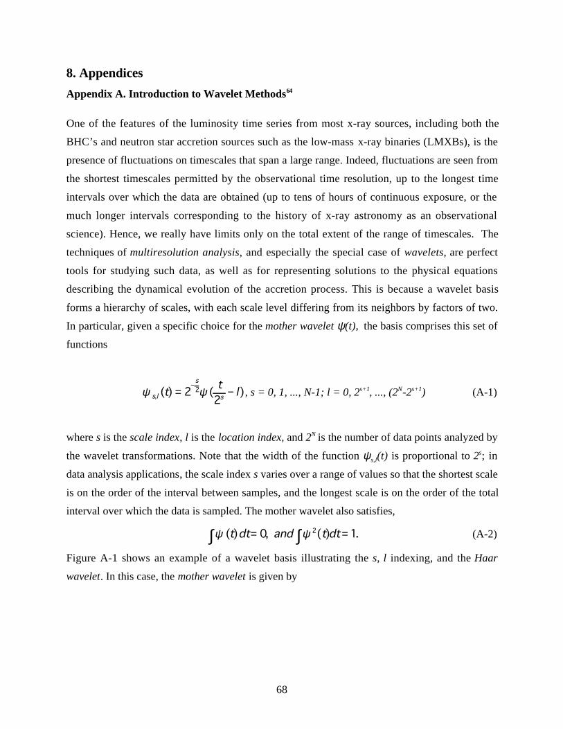
68
8. Appendices
Appendix A. Introduction to Wavelet Methods64
One of the features of the luminosity time series from most x-ray sources, including both the
BHC’s and neutron star accretion sources such as the low-mass x-ray binaries (LMXBs), is the
presence of fluctuations on timescales that span a large range. Indeed, fluctuations are seen from
the shortest timescales permitted by the observational time resolution, up to the longest time
intervals over which the data are obtained (up to tens of hours of continuous exposure, or the
much longer intervals corresponding to the history of x-ray astronomy as an observational
science). Hence, we really have limits only on the total extent of the range of timescales. The
techniques of multiresolution analysis, and especially the special case of wavelets, are perfect
tools for studying such data, as well as for representing solutions to the physical equations
describing the dynamical evolution of the accretion process. This is because a wavelet basis
forms a hierarchy of scales, with each scale level differing from its neighbors by factors of two.
In particular, given a specific choice for the mother wavelet ψ(t), the basis comprises this set of
functions
ψ ψs l
s
stt
l, ( ) ( )= −−
22
2 , s = 0, 1, ..., N-1; l = 0, 2s+1, ..., (2N-2s+1) (A-1)
where s is the scale index, l is the location index, and 2N is the number of data points analyzed by
the wavelet transformations. Note that the width of the function ψs,l(t) is proportional to 2s; in
data analysis applications, the scale index s varies over a range of values so that the shortest scale
is on the order of the interval between samples, and the longest scale is on the order of the total
interval over which the data is sampled. The mother wavelet also satisfies,
ψ ψ( ) , ( ) .t dt and t dt= =∫ ∫0 12 (A-2)
Figure A-1 shows an example of a wavelet basis illustrating the s, l indexing, and the Haar
wavelet. In this case, the mother wavelet is given by
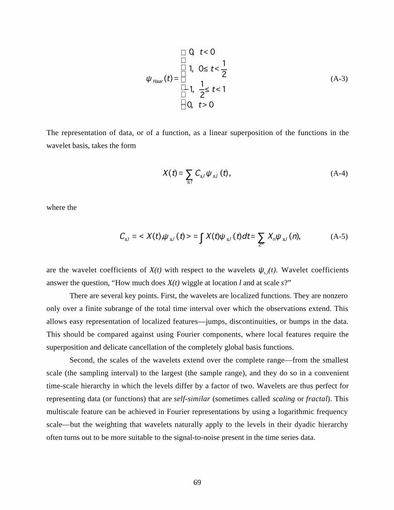
69
ψ Haar t
t
t
t
t
( )
,
,
,
,
=
<
≤ <
− ≤ <
>
0 0
1 012
112
1
0 0
(A-3)
The representation of data, or of a function, as a linear superposition of the functions in the
wavelet basis, takes the form
X t C ts ls l
s l( ) ( ),,,
,= ∑ ψ (A-4)
where the
C X t t X t t dt X ns l s l s l n s lN
, , , ,( ), ( ) ( ) ( ) ( ),= < > = = ∑∫ψ ψ ψ2
(A-5)
are the wavelet coefficients of X(t) with respect to the wavelets ψs,l(t). Wavelet coefficients
answer the question, “How much does X(t) wiggle at location l and at scale s?”
There are several key points. First, the wavelets are localized functions. They are nonzero
only over a finite subrange of the total time interval over which the observations extend. This
allows easy representation of localized features––jumps, discontinuities, or bumps in the data.
This should be compared against using Fourier components, where local features require the
superposition and delicate cancellation of the completely global basis functions.
Second, the scales of the wavelets extend over the complete range––from the smallest
scale (the sampling interval) to the largest (the sample range), and they do so in a convenient
time-scale hierarchy in which the levels differ by a factor of two. Wavelets are thus perfect for
representing data (or functions) that are self-similar (sometimes called scaling or fractal). This
multiscale feature can be achieved in Fourier representations by using a logarithmic frequency
scale––but the weighting that wavelets naturally apply to the levels in their dyadic hierarchy
often turns out to be more suitable to the signal-to-noise present in the time series data.
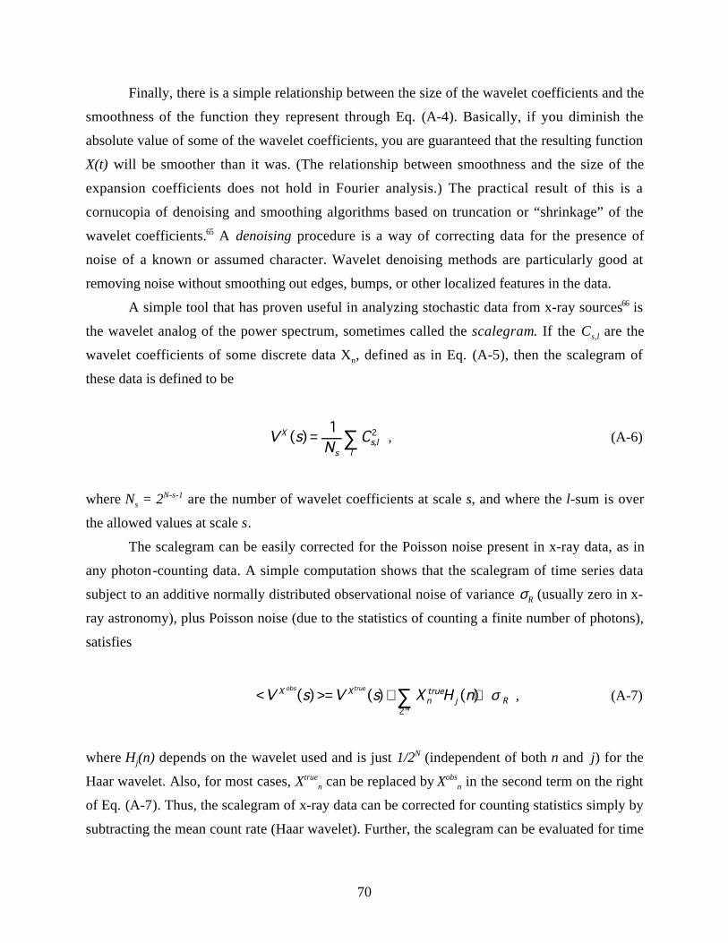
70
Finally, there is a simple relationship between the size of the wavelet coefficients and the
smoothness of the function they represent through Eq. (A-4). Basically, if you diminish the
absolute value of some of the wavelet coefficients, you are guaranteed that the resulting function
X(t) will be smoother than it was. (The relationship between smoothness and the size of the
expansion coefficients does not hold in Fourier analysis.) The practical result of this is a
cornucopia of denoising and smoothing algorithms based on truncation or “shrinkage” of the
wavelet coefficients.65 A denoising procedure is a way of correcting data for the presence of
noise of a known or assumed character. Wavelet denoising methods are particularly good at
removing noise without smoothing out edges, bumps, or other localized features in the data.
A simple tool that has proven useful in analyzing stochastic data from x-ray sources66 is
the wavelet analog of the power spectrum, sometimes called the scalegram. If the Cs,l are the
wavelet coefficients of some discrete data Xn, defined as in Eq. (A-5), then the scalegram of
these data is defined to be
V sN
CX
ss l
l
( ) ,= ∑1 2 , (A-6)
where Ns = 2N-s-1 are the number of wavelet coefficients at scale s, and where the l-sum is over
the allowed values at scale s.
The scalegram can be easily corrected for the Poisson noise present in x-ray data, as in
any photon-counting data. A simple computation shows that the scalegram of time series data
subject to an additive normally distributed observational noise of variance σR (usually zero in x-
ray astronomy), plus Poisson noise (due to the statistics of counting a finite number of photons),
satisfies
< >= + +∑V s V s X H nX Xntrue
j R
obs true
N
( ) ( ) ( ) σ2
, (A-7)
where Hj(n) depends on the wavelet used and is just 1/2N (independent of both n and j) for the
Haar wavelet. Also, for most cases, Xtruen can be replaced by Xobs
n in the second term on the right
of Eq. (A-7). Thus, the scalegram of x-ray data can be corrected for counting statistics simply by
subtracting the mean count rate (Haar wavelet). Further, the scalegram can be evaluated for time
71
series data that are arbitrarily spaced in time, including point process data (e.g., for such data as
the arrival times of individual photons).
Putting all of these features together, the scalegram and related tools seem to be very
well-suited for studying fluctuations of x-ray sources on the shortest possible timescales. This is
the kind of information that is needed for the identification and characterization of black hole
accretion. A discussion of the use of wavelets to analyze HEAO data on Cygnus X-1 for this
very signature can be found in the Snowmass ‘94, G2 working group proceedings.33
Appendix B. A Table of Black Hole Candidates67
Table B-1 contains a list of BHC that are contained in x-ray binary systems. In cases where a
mass determination (Mass Function) for the system has been obtained, it is included in the table.
The BHC without mass solutions are based on x-ray spectrum signatures that are discussed in
Sec. 4a.
9. References1 C. E. Misner, K. S. Thorne, and J. A. Wheeler, Gravitation (Freeman, San Francisco, 1973). I refer to this book asMTW.2 I. Novikov, invited plenary talk, to appear in the proceedings of the Summer Study on Particle and NuclearAstrophysics and Cosmology in the Next Millennium, June 29-July 14, 1994––Snowmass, Colorado (1995).
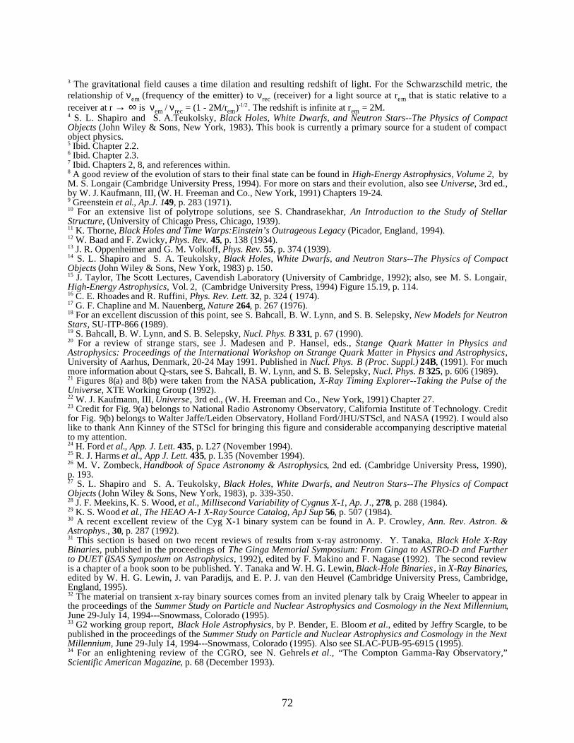
72
3 The gravitational field causes a time dilation and resulting redshift of light. For the Schwarzschild metric, therelationship of νem (frequency of the emitter) to νrec (receiver) for a light source at rem that is static relative to areceiver at r → ∞ is νem / νrec = (1 - 2M/rem)-1/2. The redshift is infinite at rem = 2M.4 S. L. Shapiro and S. A.Teukolsky, Black Holes, White Dwarfs, and Neutron Stars--The Physics of CompactObjects (John Wiley & Sons, New York, 1983). This book is currently a primary source for a student of compactobject physics.5 Ibid. Chapter 2.2.6 Ibid. Chapter 2.3.7 Ibid. Chapters 2, 8, and references within.8 A good review of the evolution of stars to their final state can be found in High-Energy Astrophysics, Volume 2, byM. S. Longair (Cambridge University Press, 1994). For more on stars and their evolution, also see Universe, 3rd ed.,by W. J. Kaufmann, III, (W. H. Freeman and Co., New York, 1991) Chapters 19-24.9 Greenstein et al., Ap.J. 149, p. 283 (1971).10 For an extensive list of polytrope solutions, see S. Chandrasekhar, An Introduction to the Study of StellarStructure, (University of Chicago Press, Chicago, 1939).11 K. Thorne, Black Holes and Time Warps:Einstein’s Outrageous Legacy (Picador, England, 1994).12 W. Baad and F. Zwicky, Phys. Rev. 45, p. 138 (1934).13 J. R. Oppenheimer and G. M. Volkoff, Phys. Rev. 55, p. 374 (1939).14 S. L. Shapiro and S. A. Teukolsky, Black Holes, White Dwarfs, and Neutron Stars--The Physics of CompactObjects (John Wiley & Sons, New York, 1983) p. 150.15 J. Taylor, The Scott Lectures, Cavendish Laboratory (University of Cambridge, 1992); also, see M. S. Longair,High-Energy Astrophysics, Vol. 2, (Cambridge University Press, 1994) Figure 15.19, p. 114.16 C. E. Rhoades and R. Ruffini, Phys. Rev. Lett. 32, p. 324 ( 1974).17 G. F. Chapline and M. Nauenberg, Nature 264, p. 267 (1976).18 For an excellent discussion of this point, see S. Bahcall, B. W. Lynn, and S. B. Selepsky, New Models for NeutronStars, SU-ITP-866 (1989).19 S. Bahcall, B. W. Lynn, and S. B. Selepsky, Nucl. Phys. B 331, p. 67 (1990).20 For a review of strange stars, see J. Madesen and P. Hansel, eds., Stange Quark Matter in Physics andAstrophysics: Proceedings of the International Workshop on Strange Quark Matter in Physics and Astrophysics,University of Aarhus, Denmark, 20-24 May 1991. Published in Nucl. Phys. B (Proc. Suppl.) 24B, (1991). For muchmore information about Q-stars, see S. Bahcall, B. W. Lynn, and S. B. Selepsky, Nucl. Phys. B 325, p. 606 (1989).21 Figures 8(a) and 8(b) were taken from the NASA publication, X-Ray Timing Explorer--Taking the Pulse of theUniverse, XTE Working Group (1992).22 W. J. Kaufmann, III, Universe, 3rd ed., (W. H. Freeman and Co., New York, 1991) Chapter 27.23 Credit for Fig. 9(a) belongs to National Radio Astronomy Observatory, California Institute of Technology. Creditfor Fig. 9(b) belongs to Walter Jaffe/Leiden Observatory, Holland Ford/JHU/STScl, and NASA (1992). I would alsolike to thank Ann Kinney of the STScl for bringing this figure and considerable accompanying descriptive materialto my attention.24 H. Ford et al., App. J. Lett. 435, p. L27 (November 1994).25 R. J. Harms et al., App J. Lett. 435, p. L35 (November 1994).26 M. V. Zombeck, Handbook of Space Astronomy & Astrophysics, 2nd ed. (Cambridge University Press, 1990),p. 193.27 S. L. Shapiro and S. A. Teukolsky, Black Holes, White Dwarfs, and Neutron Stars--The Physics of CompactObjects (John Wiley & Sons, New York, 1983), p. 339-350.28 J. F. Meekins, K. S. Wood, et al., Millisecond Variability of Cygnus X-1, Ap. J., 278, p. 288 (1984).29 K. S. Wood et al., The HEAO A-1 X-Ray Source Catalog, ApJ Sup 56, p. 507 (1984).30 A recent excellent review of the Cyg X-1 binary system can be found in A. P. Crowley, Ann. Rev. Astron. &Astrophys., 30, p. 287 (1992).31 This section is based on two recent reviews of results from x-ray astronomy. Y. Tanaka, Black Hole X-RayBinaries, published in the proceedings of The Ginga Memorial Symposium: From Ginga to ASTRO-D and Furtherto DUET (ISAS Symposium on Astrophysics, 1992), edited by F. Makino and F. Nagase (1992). The second reviewis a chapter of a book soon to be published. Y. Tanaka and W. H. G. Lewin, Black-Hole Binaries , in X-Ray Binaries,edited by W. H. G. Lewin, J. van Paradijs, and E. P. J. van den Heuvel (Cambridge University Press, Cambridge,England, 1995).32 The material on transient x-ray binary sources comes from an invited plenary talk by Craig Wheeler to appear inthe proceedings of the Summer Study on Particle and Nuclear Astrophysics and Cosmology in the Next Millennium,June 29-July 14, 1994---Snowmass, Colorado (1995).33 G2 working group report, Black Hole Astrophysics, by P. Bender, E. Bloom et al., edited by Jeffry Scargle, to bepublished in the proceedings of the Summer Study on Particle and Nuclear Astrophysics and Cosmology in the NextMillennium, June 29-July 14, 1994---Snowmass, Colorado (1995). Also see SLAC-PUB-95-6915 (1995).34 For an enlightening review of the CGRO, see N. Gehrels et al., “The Compton Gamma-Ray Observatory,”Scientific American Magazine, p. 68 (December 1993).

73
35 K. Hurley et al., Nature 372, p. 652 (1994).36 G. J. Fishman, “Gamma-ray bursts: Observational overview,” The Second Compton Symposium, AIP ConferenceProceedings 304, p. 22 (1994).37 R. J. Nemiroff, “A century of gamma-ray burst models,” AIP Proceedings 307, p. 730 (1994).38 T. Murakami et al., Nature 335, p. 234 (1988).39 Compton Observatory BATSE Second Burst Catalog (compact disc--CD). Produced by the Compton ObservatoryScience Support Center at NASA/Goddard Space Flight Center in cooperation with the BATSE Instrument Team,directory doc/into.txt (January 1, 1995).40 IBID, directory catalog/basic.txt.41 C. Meegan et al., AIP Conference Proceedings 307, p. 3 (1994).42 M. S. Briggs et al., AIP Conference Proceedings 307, p. 44 (1994).43 M. S. Briggs, ApJ, 407, p. 126 (1993).44 G. Kanbach et al.., Space Science Reviews, 46, p. 69 (1988) for the detailed description of the instrument; andD.J. Thompson, et al., Ap.J.Supp. 86, p. 629 (1993) for the instrument calibration.45 This brief description of the instrument capabilities was largely taken from Compton Observatory EGRET All-SkySurvey, Vol 1 (compact disc--CD). Produced by the Compton Observatory Science Support Center atNASA/Goddard Space Flight Center, directory doc/dos/cdrom.tex (June 1, 1994).46 D. J. Thompson et al., ApJ 436, p. 229 (1994).47 C. E. Fichtel et al., ApJS 94, p. 551 (1994).48 P. Sreekumar et al., ApJ 400, p. L67 (1992).49 C. von Montigny et al., ApJ 440, p. 525 (1995).50 E. J. Schneid et al., “High-energy solar phenomena--A new era of spacecraft measurements,” AIP ConferenceProceedings 294, edited by J. M. Ryan and W. T. Bestrand, p. 94 (1994).51 This particular argument comes from Gary Godfrey, a SLAC colleague.52 J. W. Cronin et al., Annu. Rev. Nucl. Part. Sci. 43, p. 883 (1993).53 A. D. Kerrick et al., ApJ, 438, p. L59 (1995).54 L. C. Lamb et al., Ground Based Astronomy, R2 working group report, Summer Study on Particle and NuclearAstrophysics and Cosmology in the Next Millennium, June 29-July 14, 1994---Snowmass, Colorado, EFI Preprint96-14, Enrico Fermi Institute, University of Chicago, to appear in the proceedings of the workshop (1995).55 R. Much, Ph. D. Thesis, Max Planck Institut für Extraterrestriche Physik.56 O. C. De Jager et al., in preparation (1995).57 O. C. De Jager and A. K. Harding, ApJ 396, p. 161 (1992).58 F. W. Stecker et al., ApJ 390, p L49 (1992).59 D. MacMinn and J. Primack, submitted to ApJ Lett (1994).60 The GLAST Team currently includes members from the following institutions, in alphabetical order: Enrico FermiInstitute, University of Chicago; Kanagawa University, Japan; Lockheed Research Laboratory, Palo Alto, CA;University of Maryland; Max Planck Institut für Extraterrestriche Physik, Garching, Germany; NASA AmesResearch Center, Mountain View, CA; Naval Research Center, Washington DC; University of California at SantaCruz; Sonoma State University; Stanford University, HEPL, Physics Department, and SLAC; University of Tokyo,Japan; Istituto Nazionale di Fisica Nucleare, Trieste, Italy; University of Washington.61 For a recent review of the GLAST project, see Elliott D. Bloom, GLAST, invited talk presented at the InternationalHeidelberg Workshop on TeV Gamma-Ray Astrophysics, Heidelberg, Germany, October 3-7, 1994. To be publishedin Space Science Reviews. Also see SLAC-PUB-95-6738 (1995).62 Bill Atwood (private communication, 1994).63 I. Novikov, Black Holes and the Universe, (Cambridge University Press, 1990). (Paperbound. ISBN:0-521-36683-6.)64 J. Scargle, much of Sec. 3.2 of Ref. 33 and private communication (1994).65 David Donoho and Ian Johnstone of Stanford University have written a number of papers on wavelet denoisingthat are available over the Internet via FTP at playfair.stanford.edu; theoretical papers are in the directory/pub/reports, abstracts in pub/reports/Abstracts, and a MatLab software package developed with Jeff Scargle inthe directory /pub/software/wavelets. MatLab is a trademark of The MathWorks, Inc.66 J. D. Scargle et al., ApJ Lett. 411, p. L91 (1993).67 Y. Tanaka and W. H. G. Lewin, “Black-hole binaries,” in X-Ray Binaries, edited by W. H. G. Lewin,J. van Paradijs, and E. P. J. van den Heuvel (Cambridge University Press, Cambridge, England, 1995).
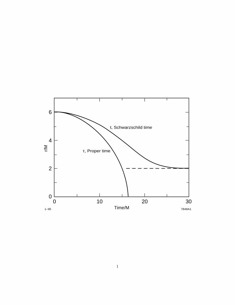
1–95 7848A1
τ, Proper time
t, Schwarzschild time
00
2
4
6
10Time/M
r/M
20 30
1
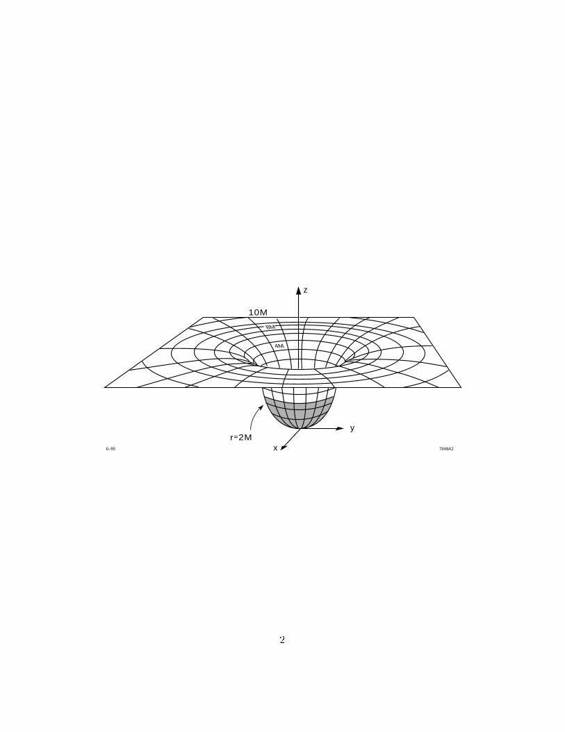
y
x6–95 7848A2
z
4M
8M
r=2M
10M
2
Log Density (kg/m3)1–95 7848A3
Lo
g P
ress
ure
(
Pa)
73
Pc ∝ρc4/3
Pc ∝ρc5/3
1.5 M
0.8 M
10
20
30
11 15
Gravity
3
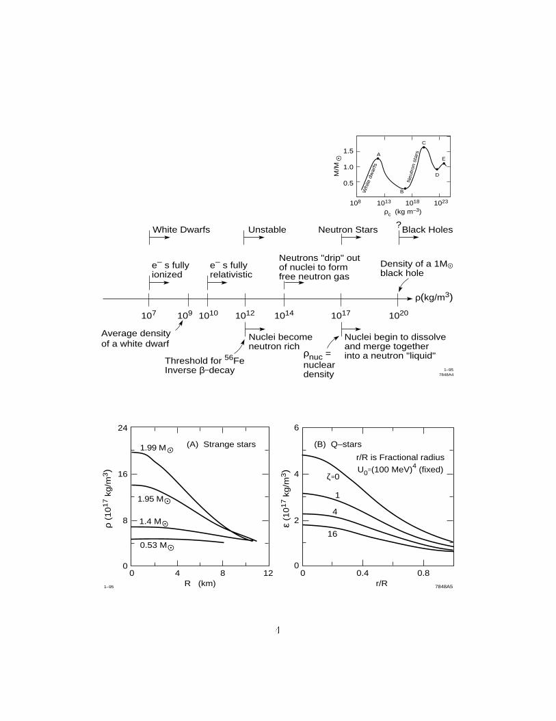
1.5C
A
Whi
te d
war
fs
Neutr
on s
tars
B
E
D
1.0
0.5
108 1013 1018
ρc (kg m–3)1023
White Dwarfs
e– s fully ionized
e– s fully relativistic
Unstable Neutron Stars
1020101710141012
ρ(kg/m3)
Neutrons "drip" outof nuclei to form free neutron gas
Nuclei begin to dissolveand merge togetherinto a neutron "liquid"
Black Holes?
Density of a 1Mblack hole
Nuclei becomeneutron rich
Threshold for 56FeInverse β–decay
ρnuc = nucleardensity
1010
Average densityof a white dwarf
109107
1–957848A4
M/M
r/R 7848A5
0
2
0.40 0.8
4
6
(B) Q–stars
r/R is Fractional radius
U0=(100 MeV)4 (fixed)
16
4
1
ζ=0
ε (1
017 k
g/m
3)
R (km)1–95
0
8
16
24
8 124
(A) Strange stars
0.53 M
1.4 M
1.95 M
1.99 M
0
ρ (1
017 k
g/m
3)
4
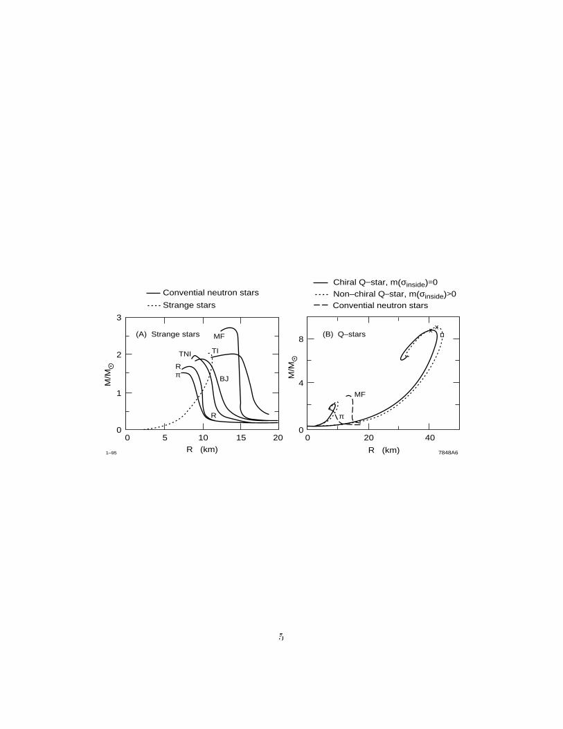
R (km) 7848A61–95
0
1
15 20105
2
3
MF
Convential neutron stars
Strange stars
TNI
R
R
BJπ
TI
Non–chiral Q–star, m(σinside)>0Convential neutron stars
Chiral Q–star, m(σinside)=0
R (km)
00 20 400
4
8
MF
π
(B) Q–stars(A) Strange stars x x
M/M
M/M
5
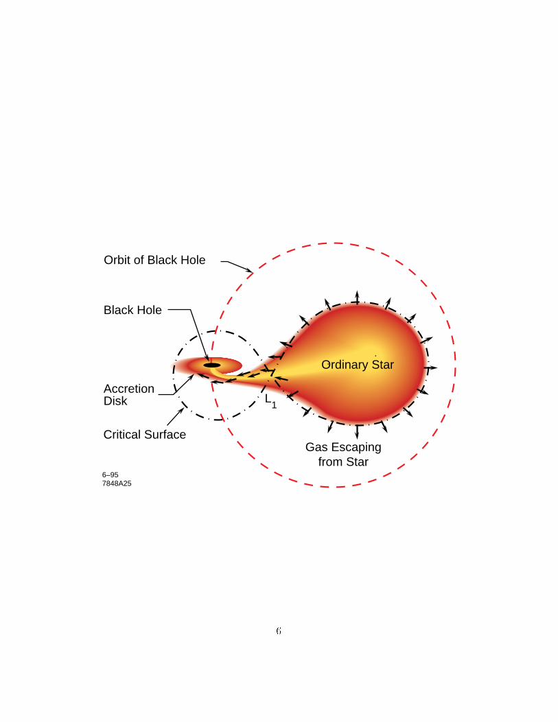
Orbit of Black Hole
Black Hole
Critical Surface
L1
Ordinary Star
6–957848A25
AccretionDisk
Gas Escapingfrom Star
6
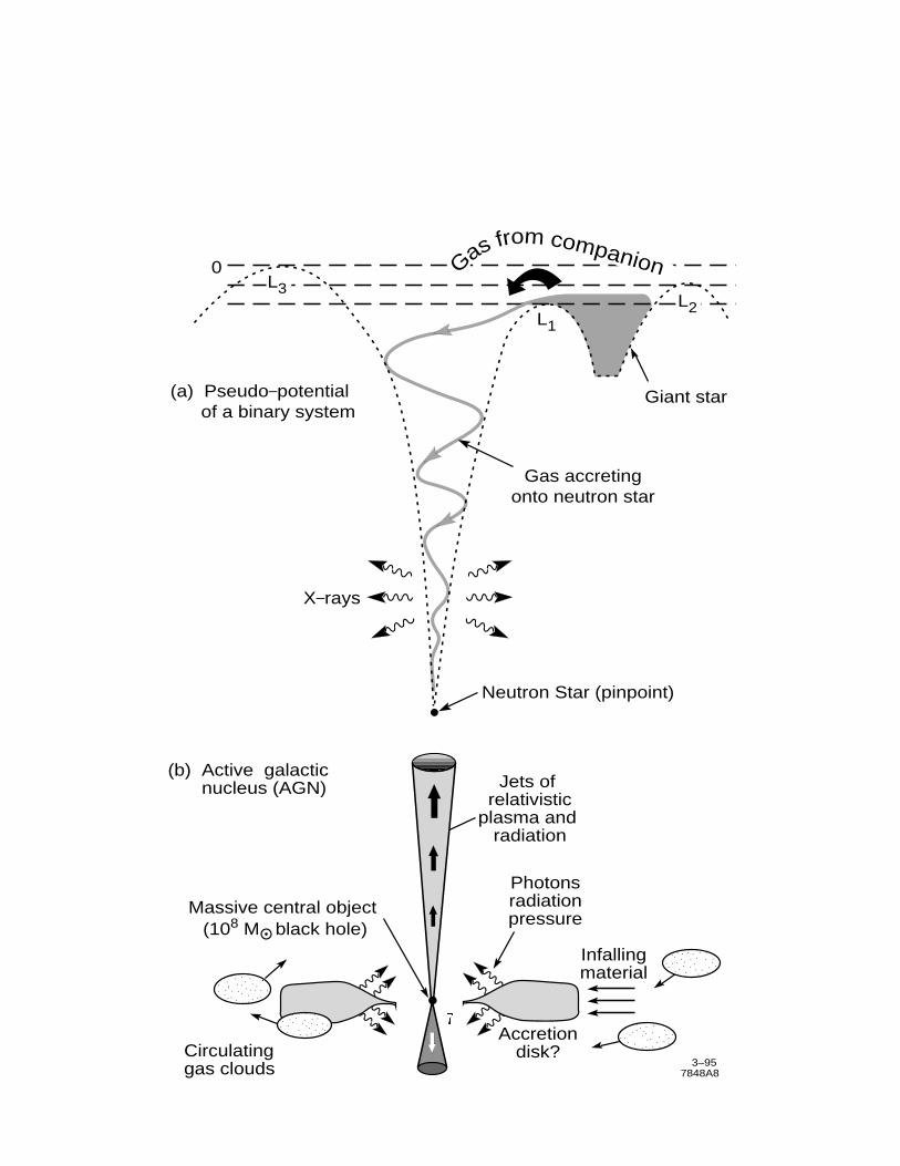
Giant star(a) Pseudo–potential of a binary system
X–rays
Neutron Star (pinpoint)
0
Gas accretingonto neutron star
L2L1
Gas from companion
Jets of relativistic
plasma and radiation
Photonsradiationpressure
Infallingmaterial
(b) Active galactic nucleus (AGN)
������
�����
Massive central object (108 M black hole)
Accretiondisk?Circulating
gas clouds 7848A83–95
L3
7
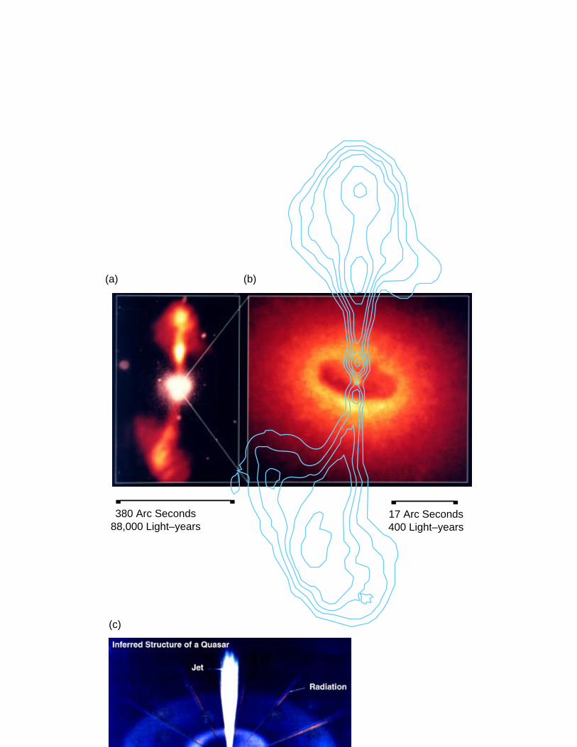
17 Arc Seconds400 Light–years
380 Arc Seconds88,000 Light–years
(b)(a)
(c)
8
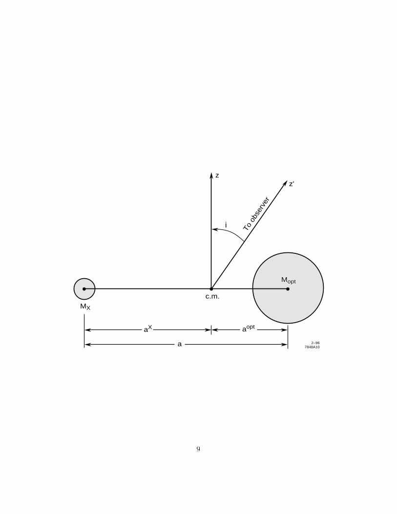
c.m.MX
aopt
2–967848A10
z'z
i
To o
bser
ver
a
aX
MoptMopt
9
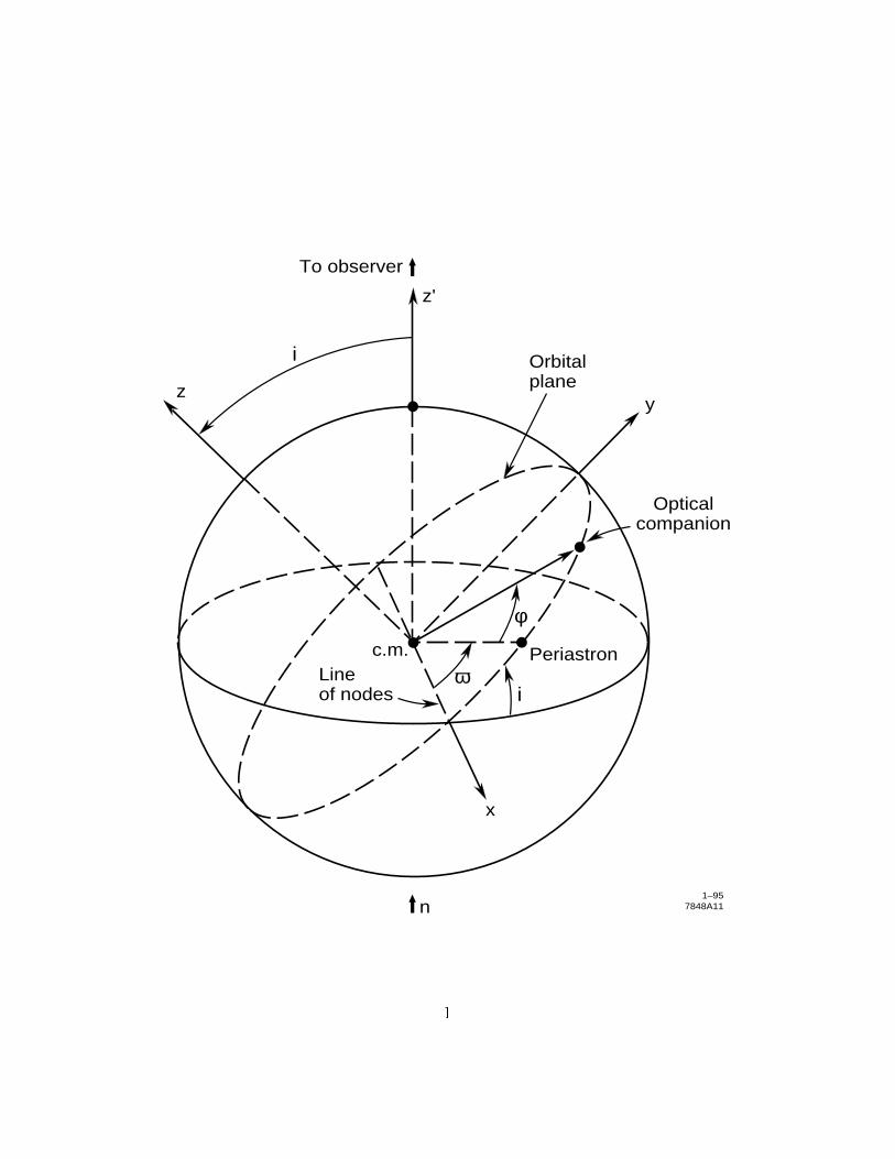
PeriastronLine of nodes
c.m.
Orbital plane
y
Opticalcompanion
i
x
n1–95
7848A11
φ
ω
z'
z
i
To observer
1
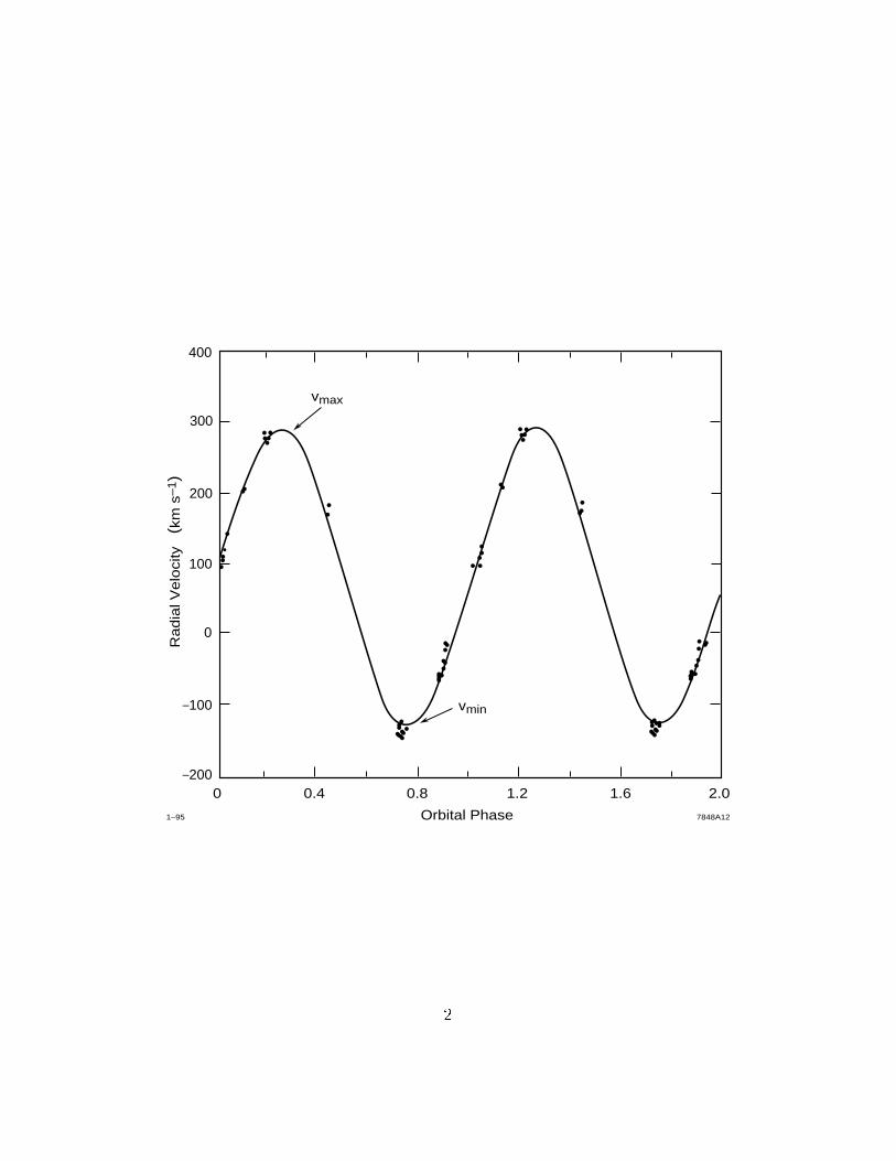
1–95 7848A12
vmin
vmax
0.40
0
–100
–200
Orbital Phase
Radia
l Velo
city
(
km s
–1)
1.61.2 2.00.8
100
200
300
400
2
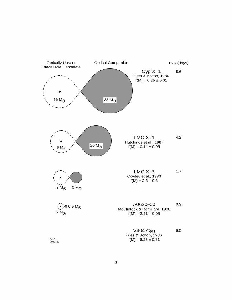
Optical CompanionOptically UnseenBlack Hole Candidate
Cyg X–1Gies & Bolton, 1986f(M) = 0.25 ± 0.01
Porb (days)
5.6
A0620–00McClintock & Remillard, 1986
f(M) = 2.91 ± 0.08
LMC X–3Cowley et al., 1983
f(M) = 2.3 ± 0.3
0.3
V404 CygGies & Bolton, 1986f(M) = 6.26 ± 0.31
6.5
1.7
LMC X–1Hutchings et al., 1987
f(M) = 0.14 ± 0.05
4.2
16 M
6 M
9 M 6 M
9 M
0.5 M
33 M
20 M
7848A133–95
3
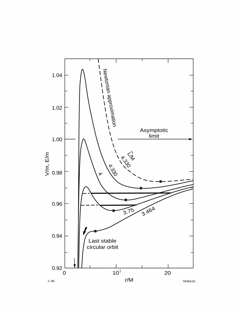
1–95 7848A16
10
V/m
, E
/m
Asymptoticlimit
Last stablecircular orbit
3.4643.75
r/M0
0.94
0.9220
0.96
0.98
4.3304.33041.00
1.02
1.04
New
tonian approximation
L/M
4
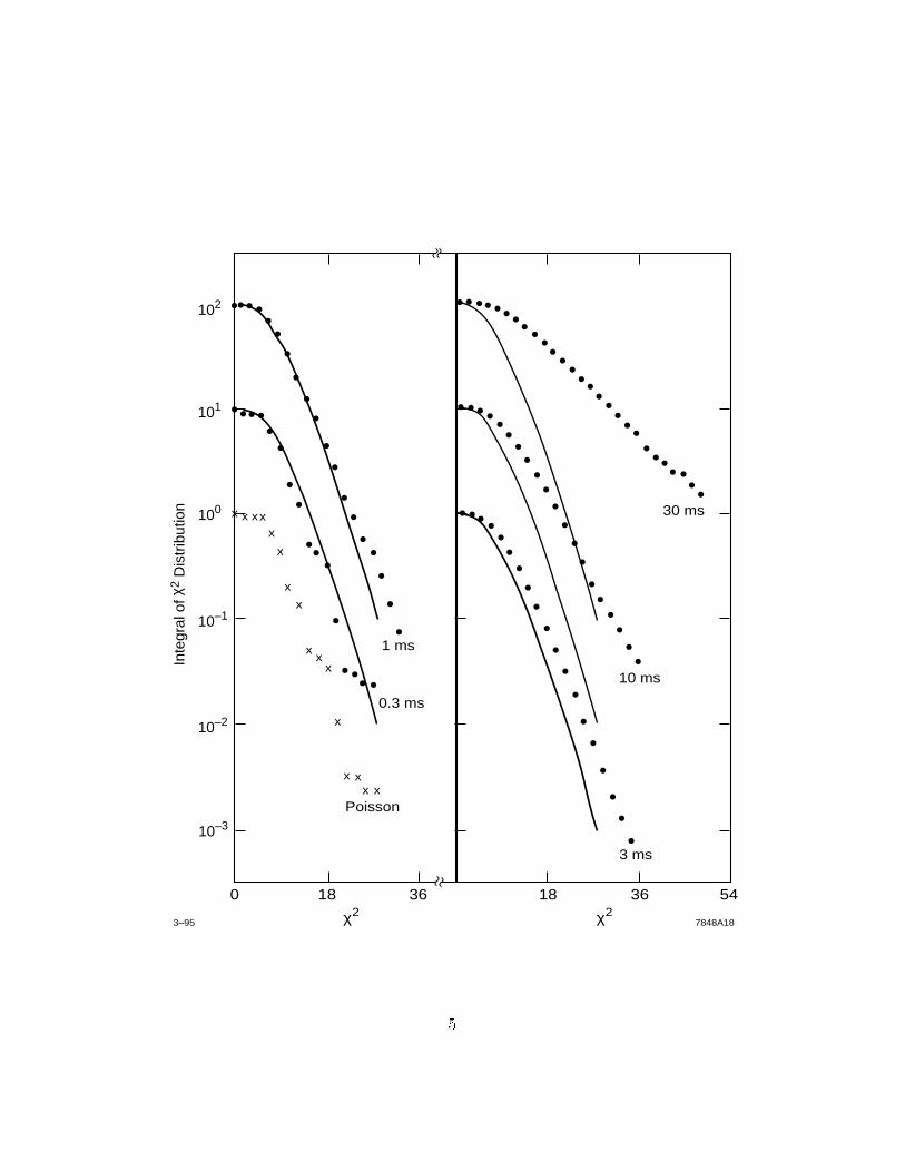
3–95 7848A18χ2χ218
Poisson
0.3 ms
1 ms
10 ms
3 ms
30 ms
0
10–2
10–1
100
101
102
10–3
Inte
gral
of χ
2 D
istr
ibut
ion
36 18 36 54
xxx
x
xx
x
x
x
x
xxxxx
x
5
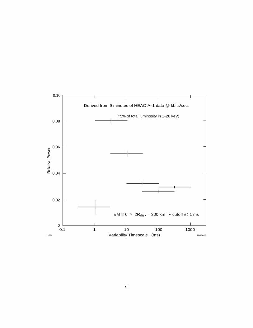
7848A191–95
10Variability Timescale (ms)
Derived from 9 minutes of HEAO A–1 data @ kbits/sec.
100 100010.10
0.08
0.06
0.04
0.02
0.10
Rel
ativ
e P
ower
(~5% of total luminosity in 1–20 keV)
r/M ~ 6 2Rdisk = 300 km cutoff @ 1 ms=
6
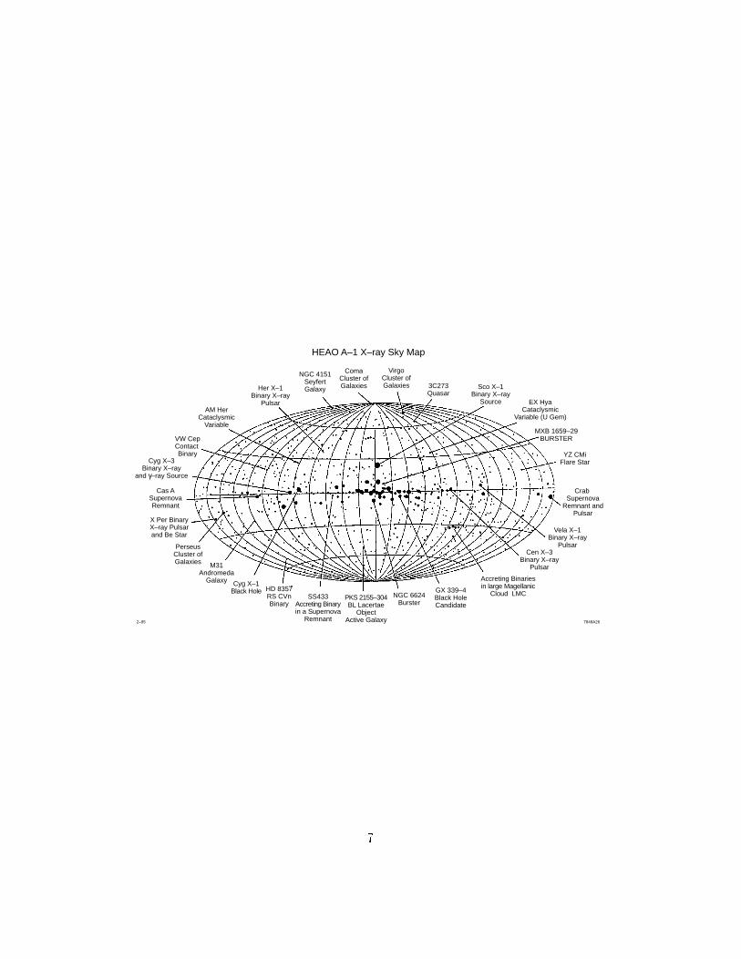
SS433Accreting Binaryin a Supernova
Remnant
Crab Supernova
Remnant andPulsar
Vela X–1Binary X–ray
PulsarCen X–3
Binary X–rayPulsar
Accreting Binariesin large Magellanic
Cloud LMC
Cas ASupernovaRemnant
X Per BinaryX–ray Pulsarand Be Star
Her X–1Binary X–ray
Pulsar
Sco X–1Binary X–ray
Source
PKS 2155–304BL Lacertae
ObjectActive Galaxy
NGC 6624Burster
HD 8357RS CVnBinary
Cyg X–1Black Hole
Cyg X–3Binary X–ray
and γ–ray Source
VW CepContact Binary
AM HerCataclysmic
Variable
EX HyaCataclysmic
Variable (U Gem)
M31Andromeda
Galaxy
NGC 4151SeyfertGalaxy
PerseusCluster ofGalaxies
ComaCluster ofGalaxies
VirgoCluster ofGalaxies 3C273
Quasar
MXB 1659–29BURSTER
YZ CMiFlare Star
GX 339–4Black HoleCandidate
HEAO A–1 X–ray Sky Map
2–95 7848A26
7
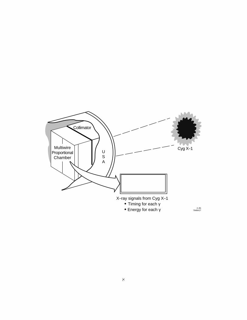
MultiwireProportionalChamber
Collimator
Cyg X–1USA
X–ray signals from Cyg X–1 Timing for each γ Energy for each γ 2–95
7848A27
8
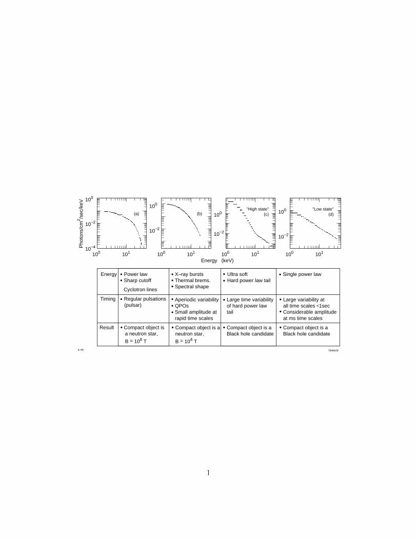
10–4
10–2
100
Energy Power law Sharp cutoff
Cyclotron lines
Ultra softHard power law tail
Timing Regular pulsations (pulsar)
X–ray burstsThermal brems.Spectral shape
Aperiodic variability QPOsSmall amplitude atrapid time scales
10–2
100
10–2
100
10–2
100
Pho
tons
/cm
2 /sec
/keV
100 100101 101 100 101 100 101
Energy (keV)
6–95 7848A28
(b)"High state"
(c)"Low state"
(d)(a)
Large time variability of hard power lawtail
Compact object is a Black hole candidate
Compact object is a neutron star,
B ~ 104 T
Single power law
Large variability at all time scales <1secConsiderable amplitudeat ms time scales
Compact object is a Black hole candidate
Result Compact object is a neutron star, B ~ 108 T ~ ~
1
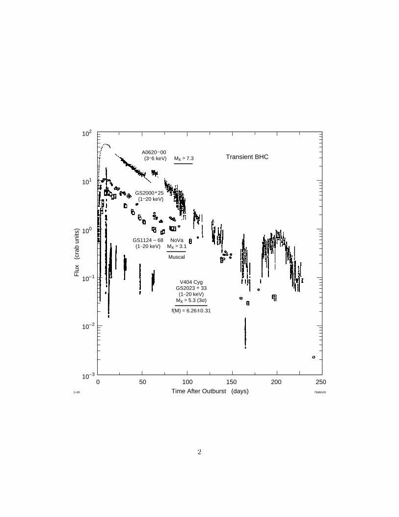
100
V404 CygGS2023 + 33
(1–20 keV)Mx > 5.3 (3σ)
f(M) = 6.26±0.31
NoVaMx > 3.1
50
Time After Outburst (days)
Flu
x (
crab
uni
ts)
Transient BHC
200 250150010–3
10–2
10–1
100
101
102
2–95 7848A29
GS1124 – 68(1–20 keV)
GS2000+25 (1–20 keV)
A0620–00 (3–6 keV) Mx > 7.3
Muscal
2
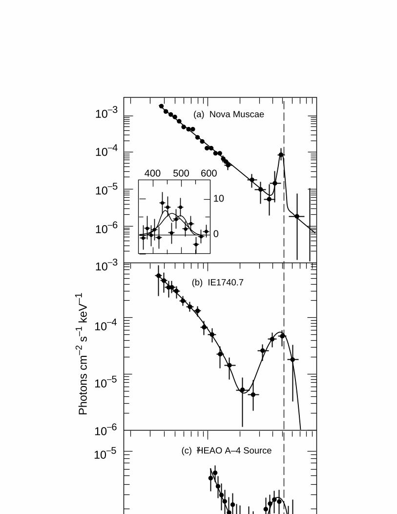
10–5
10–4
10–3
400 500 600
10
0
10–6
10–5
10–5
10–3 (a) Nova Muscae
(b) IE1740.7
(c) HEAO A–4 Source
10–4
10–6
Pho
tons
cm
–2 s
–1 k
eV–1
3
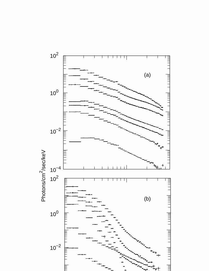
10–4
10–2
100
10–2
100
Pho
tons
/cm
2 /sec
/keV
102
102
(a)
(b)
4
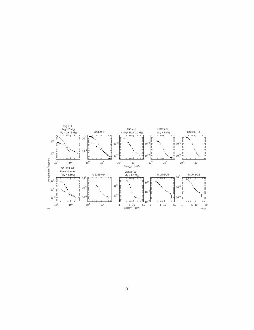
10–3
10–1
101
10–2
10–4
100
Pho
tons
/cm
2 /sec
/keV
100 101100 101
2–95 7848A31
10–2
100
1 5 10 50Energy (keV)
Energy (keV)
1 5 10 50 1 5 10 50
10–4
10–2
100
10–4
10–2
100
GS1124–68 Nova Muscae
MX > 3.1M
10–410–2
100
Cyg X–1MX > 7 M
MX = 16±5 M
10–2
10–2
100
100 101100 101100 101 100 101 100 101
10–4
10–2
10–4
10–2
LMC X–14 M < MX < 10 M
LMC X–3MX > 9 MGX339–4 GS2000+25
A0620–00MX > 7.3 M M1743–32M1705–25GS1354–64
5

6
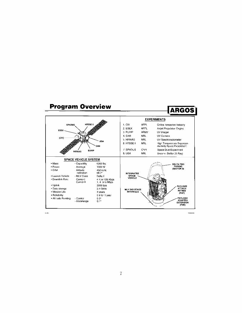
4–95 7848A56
7
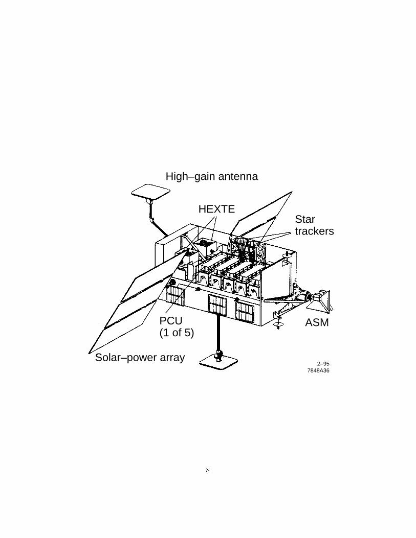
High–gain antenna
HEXTE
Solar–power array
ASMPCU (1 of 5)
Startrackers
2–957848A36
8
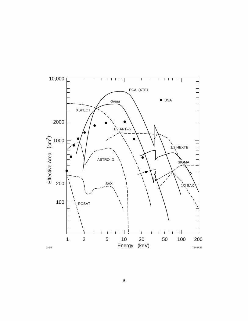
100
200
1000
10,000
Effe
ctiv
e A
rea
(cm
2 )
2000
1 2
ROSAT
ASTRO–D
USA
PCA (XTE)
Ginga
SAX
5 10 20 100 20050
2–95 7848A37Energy (keV)
1/2 SAX
1/2 ART–S
1/2 HEXTE
SIGMA
XSPECT
9
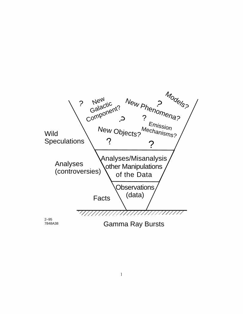
�������
?
?
?
Facts
Observations(data)
Gamma Ray Bursts
WildSpeculations
2–957848A38
Analyses(controversies)
New Objects?
New Phenomena?EmissionMechanisms?
Models?New
Galactic
Component?
Analyses/Misanalysisother Manipulations
of the Data
?
?
?
1
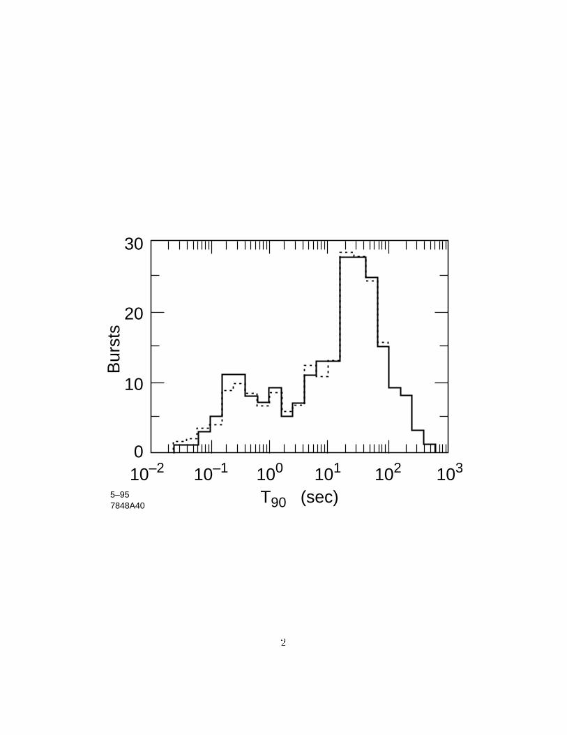
T90 (sec)7848A405–95
10
010–2 10–1 100 101 102 103
20
30
Bur
sts
2
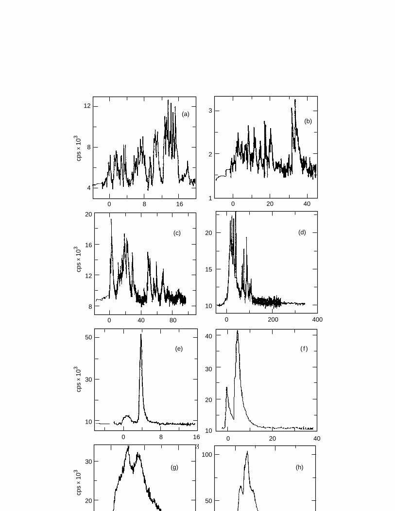
20
30
cps
x 10
3
(g)
100
50
(h)
10
30
50
cps
x 10
3
0 8 16
(e)
10
20
30
40
0 20 40
( f )
8
12
16
20
cps
x 10
3
0 40 80
(c)
10
15
20
0 400200
(d)
cps
x 10
3
0 8 16
8
12
4
(a)
1
2
3
0 20 40
(b)
3
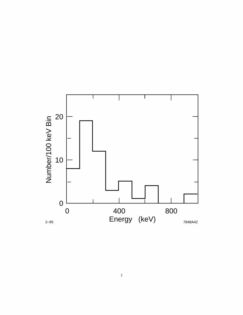
00
10
20
Num
ber/
100
keV
Bin
400Energy (keV)2–95 7848A42
800
4
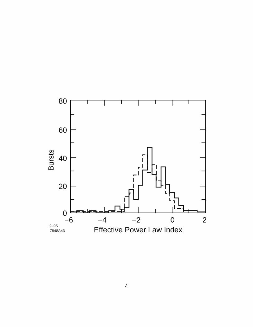
00
20
40
60
80
Bur
sts
–2 2–6 –4Effective Power Law Index
2–957848A43
5
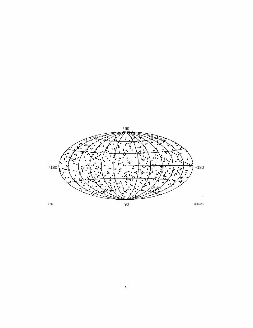
+180
2–95
–180
–90
+90
7848A44
6
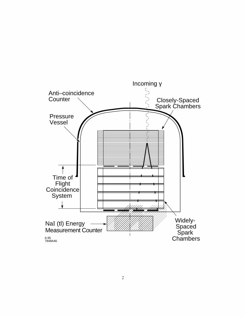
���������
������
Time ofFlight
CoincidenceSystem
NaI (tl) Energy Measurement Counter
Anti–coincidenceCounter Closely-Spaced
Spark Chambers
Incoming γ
Widely- SpacedSpark
Chambers6-957848A46
PressureVessel
7
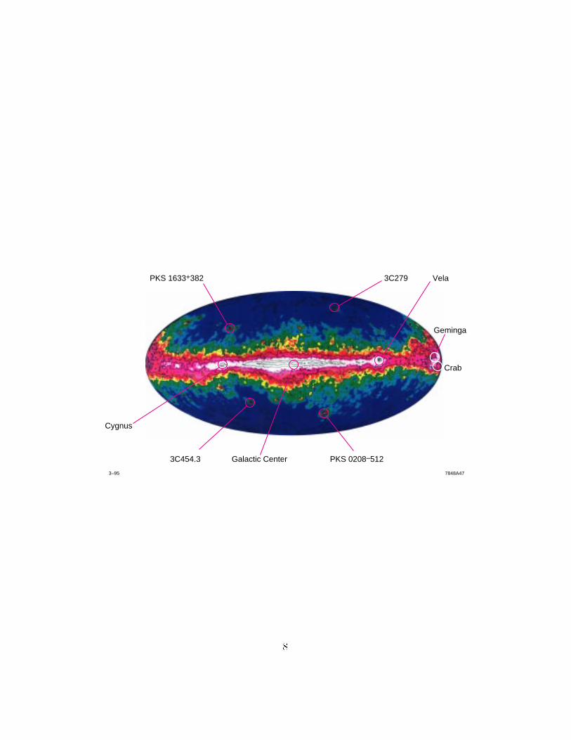
3–95 7848A47
Geminga
Crab
PKS 0208–512
PKS 1633+382 3C279 Vela
3C454.3
Cygnus
Galactic Center
8
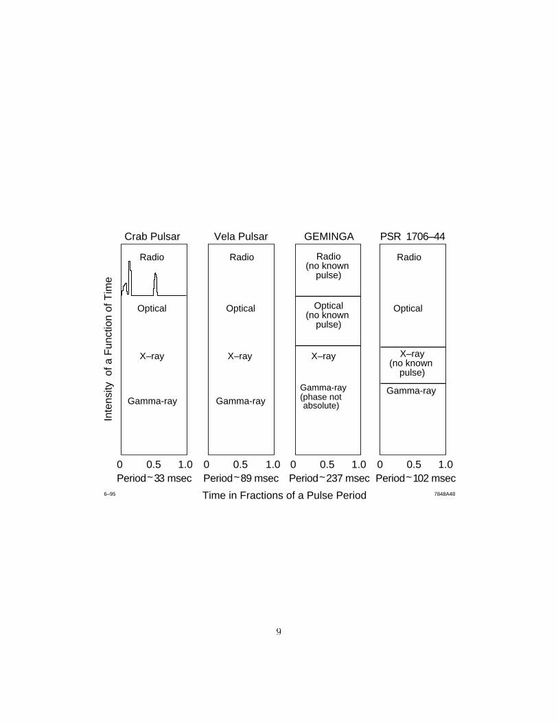
0 0.5Period ~ 33 msec
1.0 0 0.5Period ~ 89 msec
1.0 0 0.5Period ~ 237 msec
1.0 0 0.5Period ~ 102 msec
1.0
7848A486–95
Gamma-ray Gamma-ray
X–ray X–ray
Optical Optical
Radio Radio
Crab Pulsar Vela Pulsar
Time in Fractions of a Pulse Period
Inte
nsity
of a
Fun
ctio
n of
Tim
e
Gamma-ray(phase not
X–ray
GEMINGA
Gamma-ray
X–ray(no known
pulse)
Radio(no known
pulse)
Optical(no known
pulse)
Optical
Radio
PSR 1706–44
absolute)
9
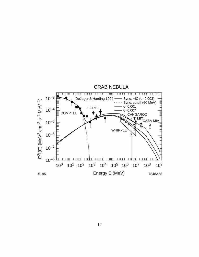
x xx
xx
x
COMPTEL
10–3
100 101 102 103 104 105
Energy E (MeV)
E2 I
(E)
( MeV
2 cm
–2 s
–1 M
eV–1
)
106 107 108 109
10–4
10–5
10–6
10–7
10–8
EGRET
DeJager & Harding 1994 Sync. +IC (σ=0.003)Sync. cutoff (60 MeV)σ=0.001σ=0.007
CANGAROO
WHIPPLE
TIBETCASA-MIA
7848A585–95
CRAB NEBULA
10
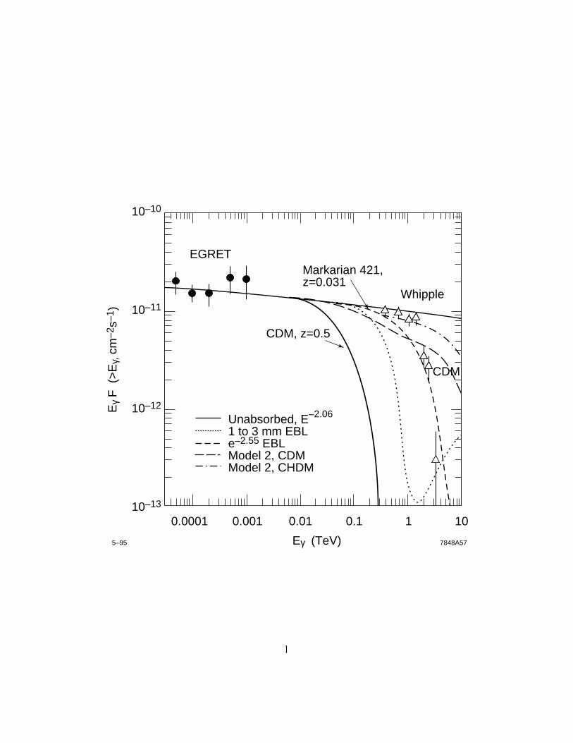
CDM, z=0.5
CDM
Markarian 421, z=0.031
Unabsorbed, E–2.06
1 to 3 mm EBLe–2.55 EBLModel 2, CDMModel 2, CHDM
Whipple
10–13
0.0001 0.001 0.01 0.1
Eγ (TeV)
Eγ
F (
>E
γ, c
m–2
s–1 )
1
7848A575–95
10
10–12
10–11
10–10
EGRET
1
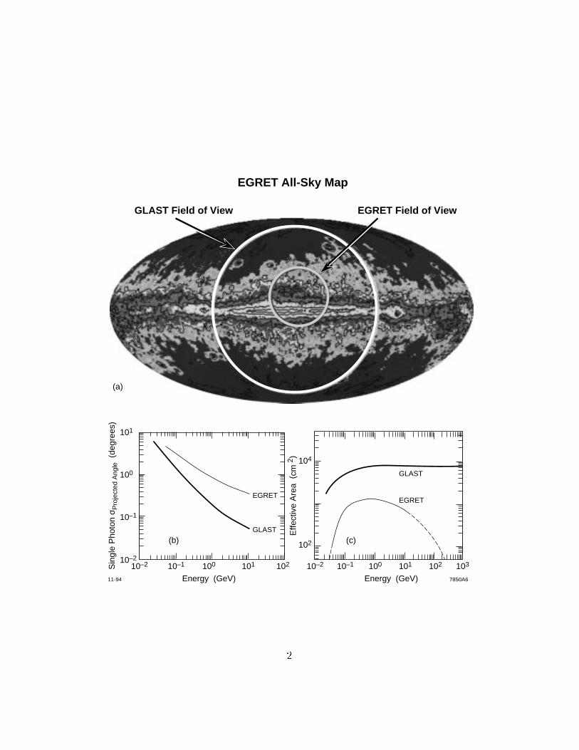
GLAST Field of View
EGRET All-Sky Map
EGRET Field of View
101
101 102
100
100
Energy (GeV)
Sin
gle
Pho
ton
σ Pro
ject
ed A
ngle
(de
gree
s)
Effe
ctiv
e A
rea
(cm
2 )
10–1
104
10–110–2
102
10–2 101 102 103100
Energy (GeV)
10–110–2
EGRETEGRET
GLAST
GLAST
(b)
(a)
(c)
11-94 7850A6
2
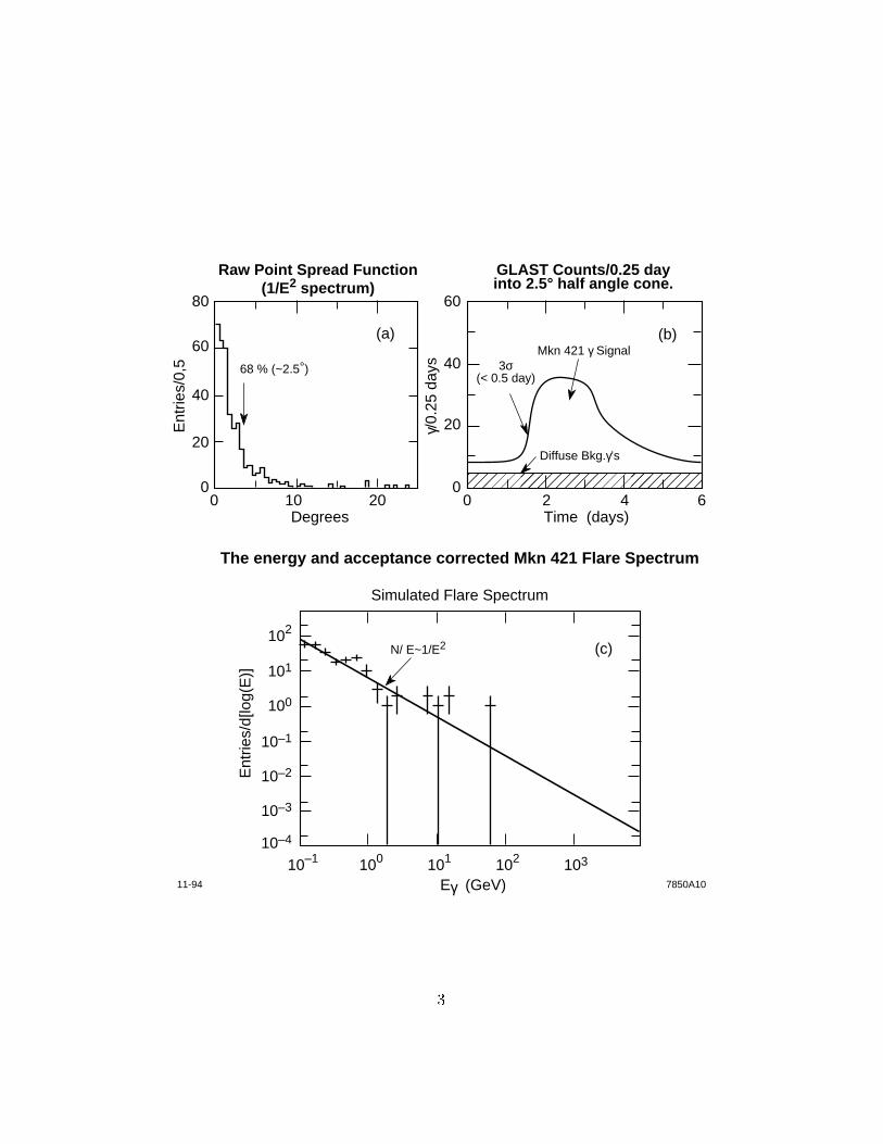
������
11-94 7850A10
(a) (b)
(c)
Mkn 421 γ Signal
0 2 4Time (days)
γ/0.
25 d
ays
Ent
ries/
0,5
60 10
10–4
100
N/ E~1/E2
10–1 101 102
Eγ (GeV)
Ent
ries/
d[lo
g(E
)]
103
10–3
10–2
10–1
100
101
102
20Degrees
Raw Point Spread Function(1/E2 spectrum)
GLAST Counts/0.25 dayinto 2.5° half angle cone.
The energy and acceptance corrected Mkn 421 Flare Spectrum
Simulated Flare Spectrum
0
20
40
60
0
20
40
80
603σ
(< 0.5 day)
Diffuse Bkg.γ’s
68 % (~2.5°)
3
7848A53 2–95
4
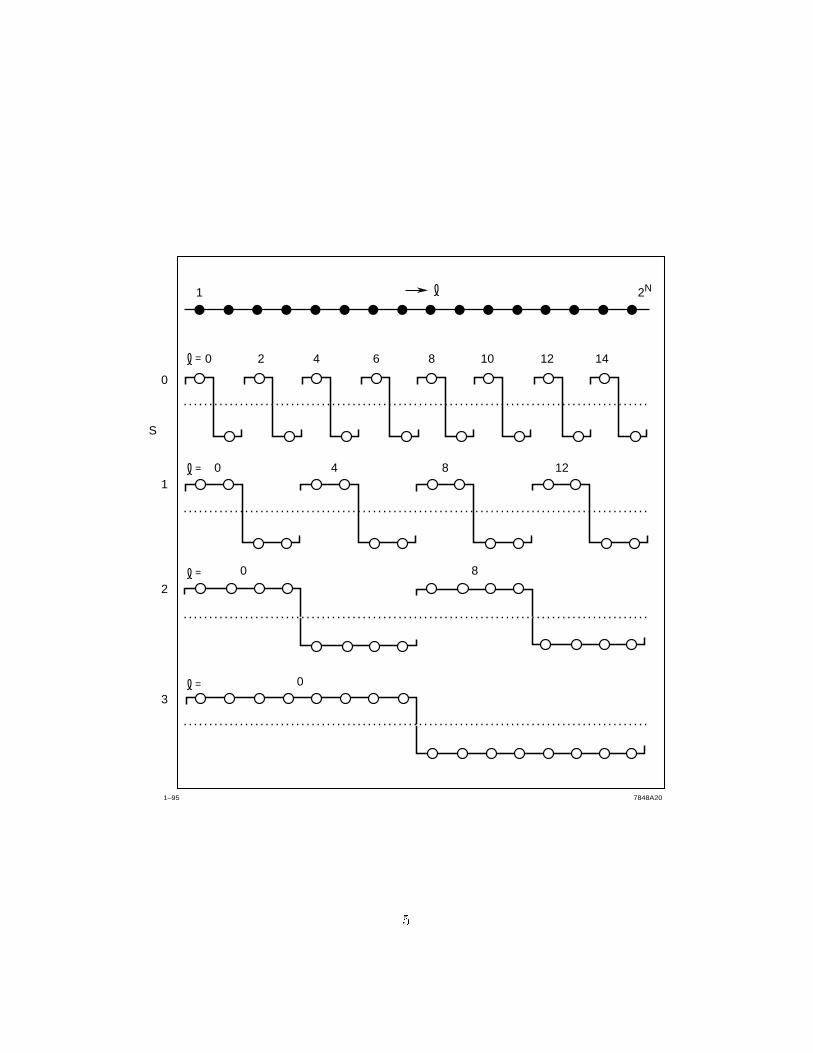
7848A201–95
0 4 8 12
12 148642 10
0 8
0
2N1
1
S
2
3
0
0=
=
=
=
5