inventory system inventory system: the set of policies and controls that monitor levels of inventory...
TRANSCRIPT
Inventory System
• Inventory system: the set of policies and controls that monitor levels of inventory and determines:– what levels should be maintained – when stock should be replenished – how large orders should be
Fixed-Order Quantity Models:Model Assumptions (Part 1)
• Demand for the product is constant and continuous throughout the period and known.
• Lead time (time from ordering to receipt) is constant.
• Price per unit of product is constant.
Fixed-Order Quantity Models:Model Assumptions (Part 2)
• Inventory holding cost is based on average inventory.
• Ordering or setup costs are constant.
• All demands for the product will be satisfied. (No back orders are allowed.)
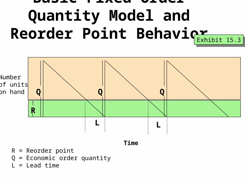
Basic Fixed-Order Quantity Model and Reorder Point
BehaviorExhibit 15.3Exhibit 15.3
R = Reorder pointQ = Economic order quantityL = Lead time
L L
Q QQ
R
Time
Numberof unitson hand
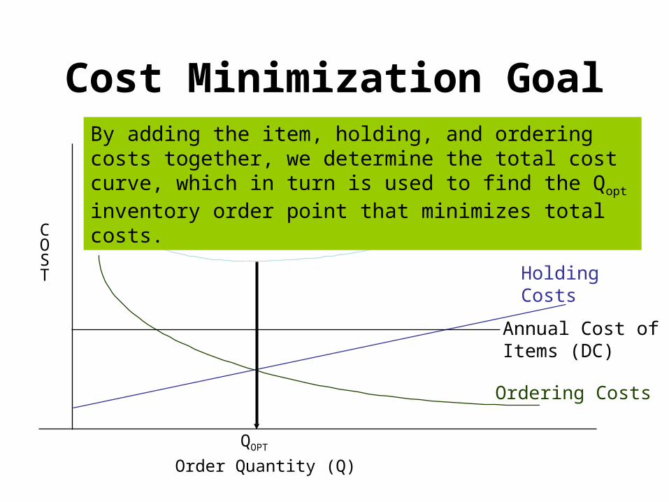
Cost Minimization Goal
Ordering Costs
HoldingCosts
QOPT
Order Quantity (Q)
COST
Annual Cost ofItems (DC)
Total Cost
By adding the item, holding, and ordering costs together, we determine the total cost curve, which in turn is used to find the Qopt inventory order point that minimizes total costs.
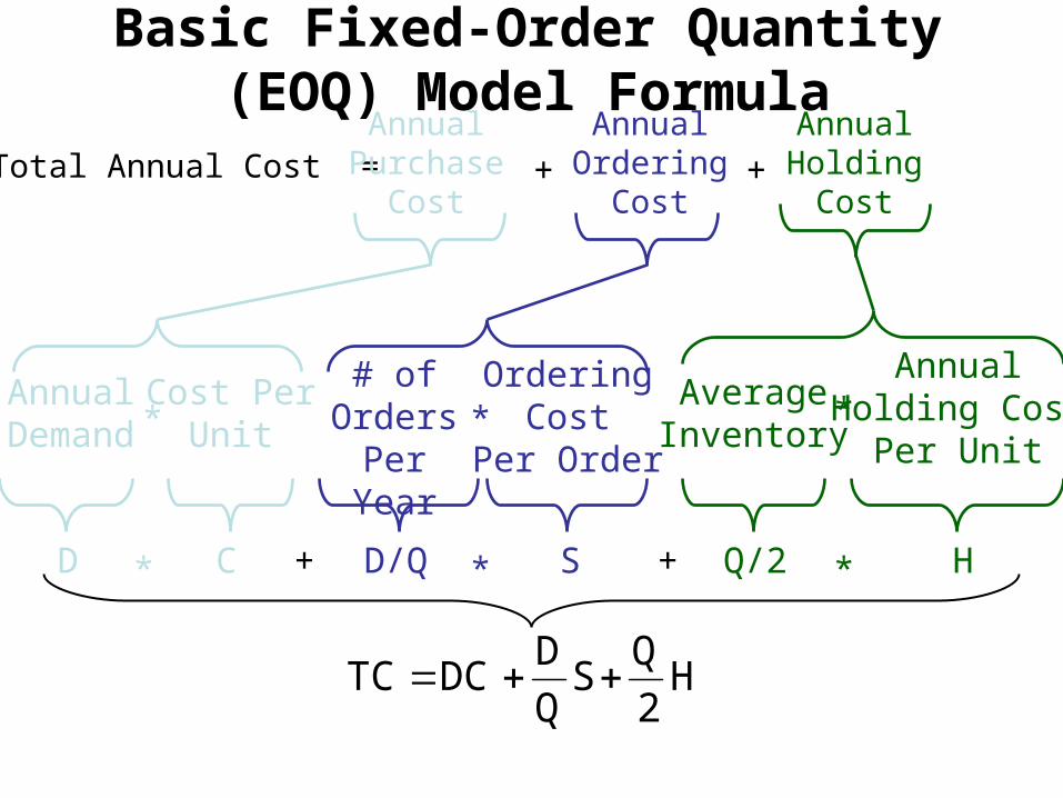
Basic Fixed-Order Quantity (EOQ) Model Formula
C* H*Q/2+S*D D/Q+
AverageInventory
AnnualHolding Cost
Per Unit*
# ofOrders
Per Year*
OrderingCost
Per Order
AnnualDemand
Cost PerUnit*
Total Annual Cost =Annual
PurchaseCost
AnnualOrdering
Cost
AnnualHolding
Cost+ +
H2
QS
Q
DDCTC
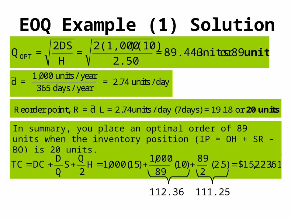
EOQ Example (1) Solution
units 89or units 89.443 = 2.50
)(10) 2(1,000 =
H
2DS = QOPT
d = 1,000 units / year
365 days / year = 2.74 units / day
Reorder point, R = d L = 2.74units / day (7days) = 19.18 or _
20 units
In summary, you place an optimal order of 89 units when the inventory position (IP = OH + SR – BO) is 20 units.
61.223,15$)5.2(2
89)10(
89
000,1)15(000,1H
2
QS
Q
DDCTC
112.36 111.25
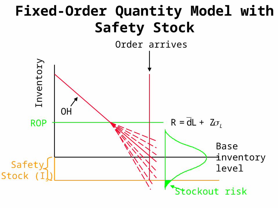
Fixed-Order Quantity Model with Safety Stock
Inve
ntor
y
ROPOH
Baseinventorylevel
Order arrives
SafetyStock (Is)
Stockout risk
Z+ Ld = R L
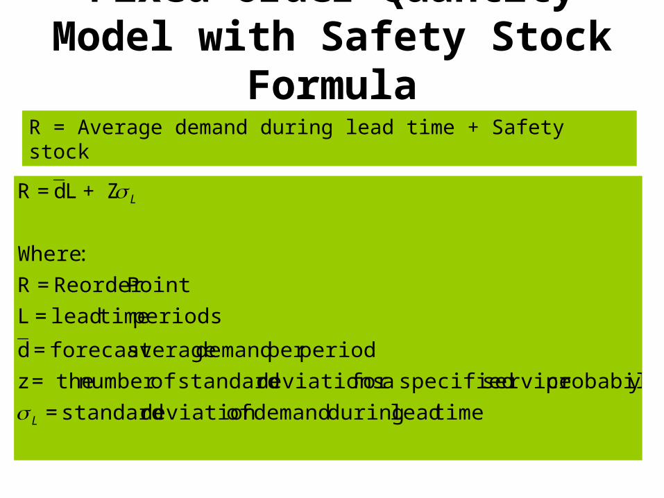
Fixed-Order Quantity Model with Safety Stock Formula
timeleadduringdemandofdeviationstandard =
yprobabilit servicespecifiedafordeviationsstandardofnumber the= z
periodper demand averageforecast = d
periods timelead = L
PointReorder = R
:Where
Z+ Ld = R
L
L
R = Average demand during lead time + Safety stock
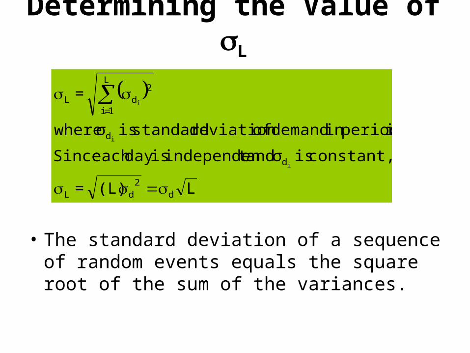
Determining the Value of L
L(L) =
constant, is σ andt independen isday each Since
i periodin demand ofdeviation standard is σ where
=
d2
dL
d
d
L
1i
2dL
i
i
i
• The standard deviation of a sequence of random events equals the square root of the sum of the variances.
Price-Break Example Problem Data
(Part 1)
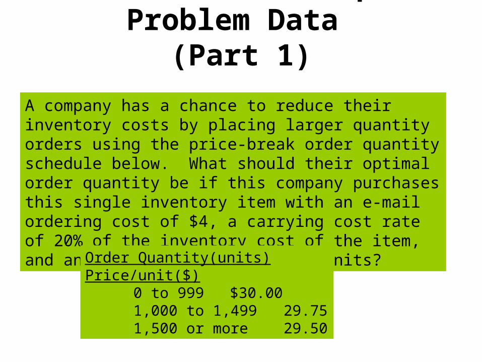
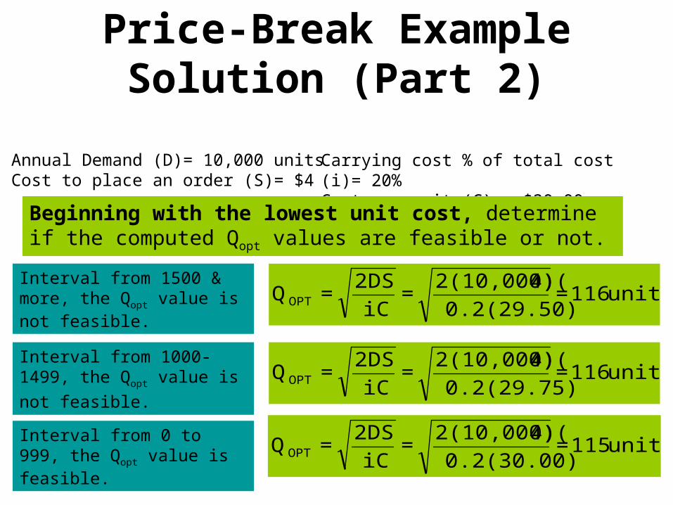
A company has a chance to reduce their inventory costs by placing larger quantity orders using the price-break order quantity schedule below. What should their optimal order quantity be if this company purchases this single inventory item with an e-mail ordering cost of $4, a carrying cost rate of 20% of the inventory cost of the item, and an annual demand of 10,000 units?
Order Quantity(units) Price/unit($)0 to 999 $30.001,000 to 1,499 29.751,500 or more 29.50
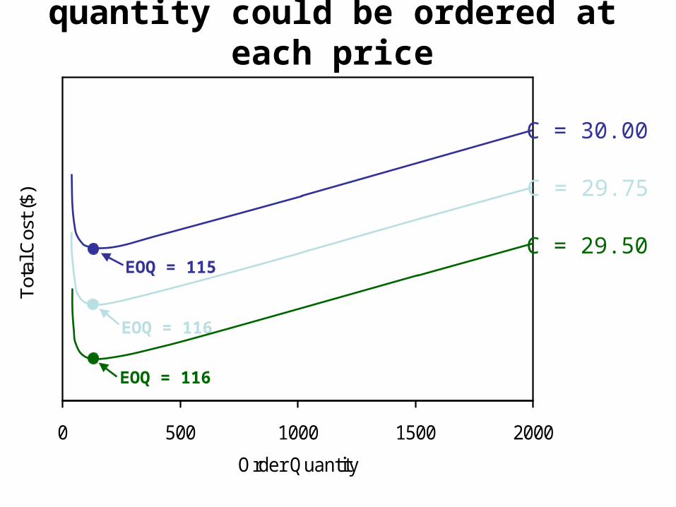
Total cost curves if any quantity could be ordered at each price
0 500 1000 1500 2000
Order Quantity
Tot
al C
ost (
$)
C = 30.00
EOQ = 115
C = 29.75
EOQ = 116
C = 29.50
EOQ = 116
Price-Break Example Solution (Part 2)
units 115 = 0.2(30.00)
4)2(10,000)( =
iC
2DS = QOPT
Annual Demand (D)= 10,000 unitsCost to place an order (S)= $4
units 116 = 0.2(29.75)
4)2(10,000)( =
iC
2DS = QOPT
units 116 = 0.2(29.50)
4)2(10,000)( =
iC
2DS = QOPT
Carrying cost % of total cost (i)= 20%Cost per unit (C) = $30.00, $29.75, $29.50
Interval from 0 to 999, the Qopt value is feasible.
Interval from 1000-1499, the Qopt value is not feasible.
Interval from 1500 & more, the Qopt value is not feasible.
Beginning with the lowest unit cost, determine if the computed Qopt values are feasible or not.

Total cost curves if any quantity could be ordered at each price
0 500 1000 1500 2000
Order Quantity
Tot
al C
ost (
$)
C = 30.00
EOQ = 115
C = 29.75
EOQ = 116
C = 29.50
EOQ = 116
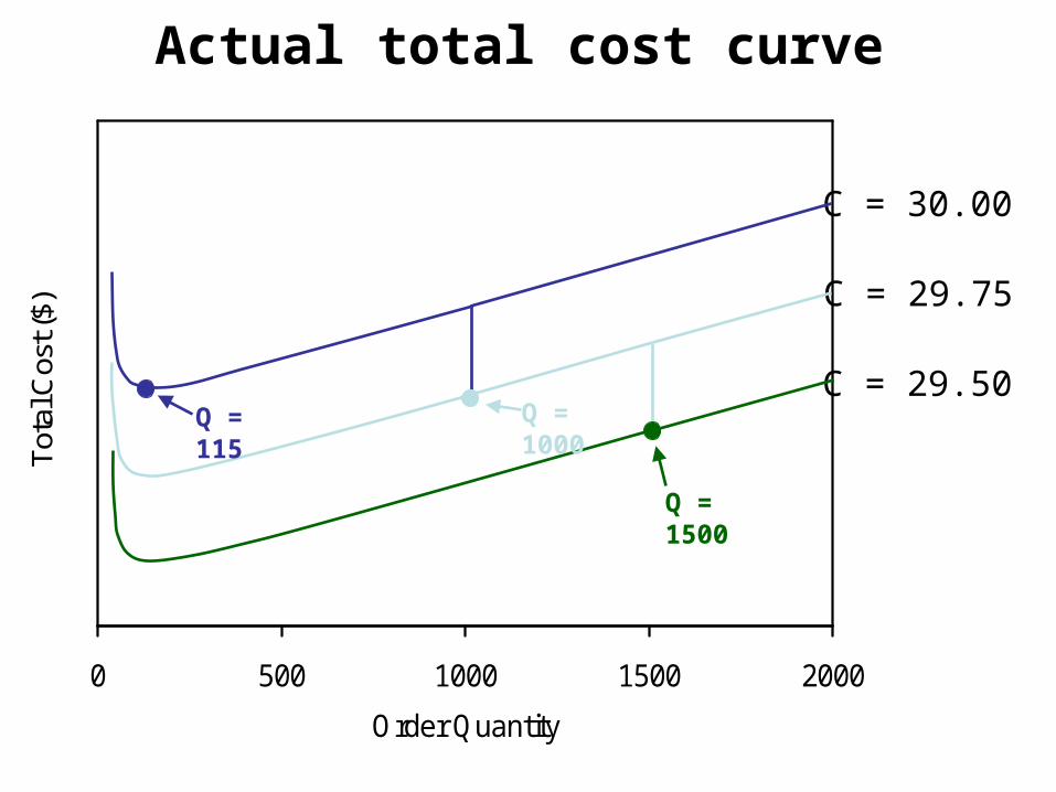
Actual total cost curve
C = 30.00
C = 29.75
C = 29.50
0 500 1000 1500 2000
Order Quantity
Tot
al C
ost (
$)
Q = 115 Q = 1000
Q = 1500
Price-Break Example Solution (Part 4)
iC 2
Q + S
Q
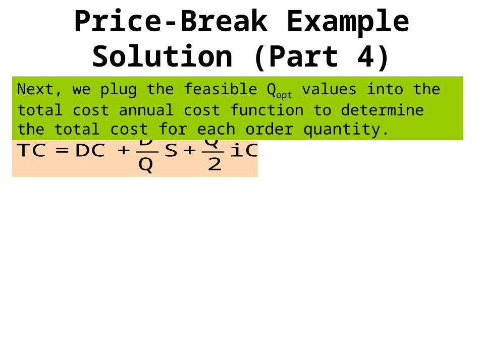
D + DC = TC
Next, we plug the feasible Qopt values into the total cost annual
cost function to determine the total cost for each order quantity.

Price-Break Example Solution (Part 5)
TC(115)= (10000*$30.00)+(10000/115)*4+(115/2)*(0.2*$30.00) = $300,693
TC(1000)= (10,000*$29.75) + (10,000/1000)*4 + (1000/2)*(0.2*$29.75) = $300,515
TC(1500) = (10,000*$29.50) + (10,000/1500)*4 + (1500/2)*(0.2*$29.50) = $299,452
Finally, we select the least costly Qopt, which is this problem occurs for an order quantity of 1500. In summary, our optimal order quantity is 1500 units.
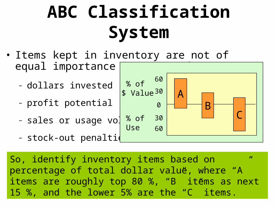
ABC Classification System• Items kept in inventory are not of equal importance
in terms of:
– dollars invested
– profit potential
– sales or usage volume
– stock-out penalties
0
30
60
30
60
AB
C
% of $ Value
% of Use
So, identify inventory items based on percentage of total dollar value, where “A” items are roughly top 80 %, “B” items as next 15 %, and the lower 5% are the “C” items.
Just-In-Time (JIT)Defined
• JIT: an integrated set of activities designed to achieve high-volume production using minimal inventories (RM, WIP, FG).
• JIT involves:– the elimination of waste in production effort.
– the timing of production resources (e.g., parts arrive at the next workstation “just in time”).
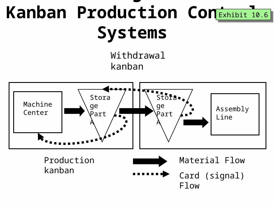
Minimizing Waste: Kanban Production Control
SystemsExhibit 10.6Exhibit 10.6
Storage Part A
Storage Part AMachine
Center Assembly Line
Material Flow
Card (signal) Flow
Withdrawal kanban
Production kanban
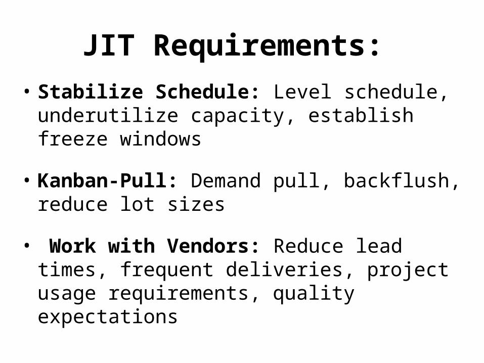
JIT Requirements:
• Stabilize Schedule: Level schedule, underutilize capacity, establish freeze windows
• Kanban-Pull: Demand pull, backflush, reduce lot sizes
• Work with Vendors: Reduce lead times, frequent deliveries, project usage requirements, quality expectations
Characteristics of JIT VendorPartnerships
• Few, nearby suppliers• Long-term contract agreements• Steady supply rate• Frequent deliveries in small lots• Buyer helps suppliers meet quality• Suppliers use process control charts• Buyer schedules inbound freight
Respect for People• Level payrolls
• Cooperative employee unions
• Subcontractor networks
• Bottom-round management style
• Quality circles (Small group involvement activities)
Goldratt’s Rules of Production Scheduling (Continued)
• Bottlenecks govern both throughput and inventory in the system.
• Transfer batch may not and many times should not be equal to the process batch.
• A process batch should be variable both along its route and in time.
• Priorities can be set only by examining the system’s constraints. Lead time is a derivative of the schedule.
Goldratt’s Theory of Constraints (TOC)
• Identify the system constraints.• Decide how to exploit the system constraints.• Subordinate everything else to that decision.• Elevate the system constraints.• If, in the previous steps, the constraints have
been broken, go back to Step 1, but do not let inertia become the system constraint.
Goldratt’s Goal of the Firm
The goal of a firm is to make money.
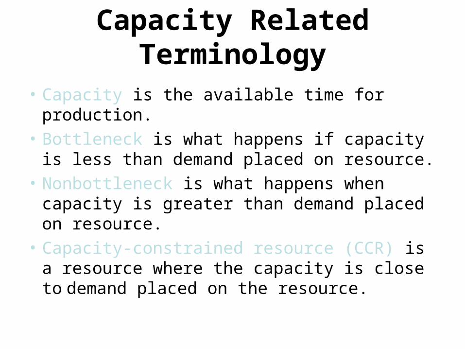
Capacity Related Terminology• Capacity is the available time for production.• Bottleneck is what happens if capacity is less
than demand placed on resource.• Nonbottleneck is what happens when capacity
is greater than demand placed on resource.• Capacity-constrained resource (CCR) is a
resource where the capacity is close to demand placed on the resource.
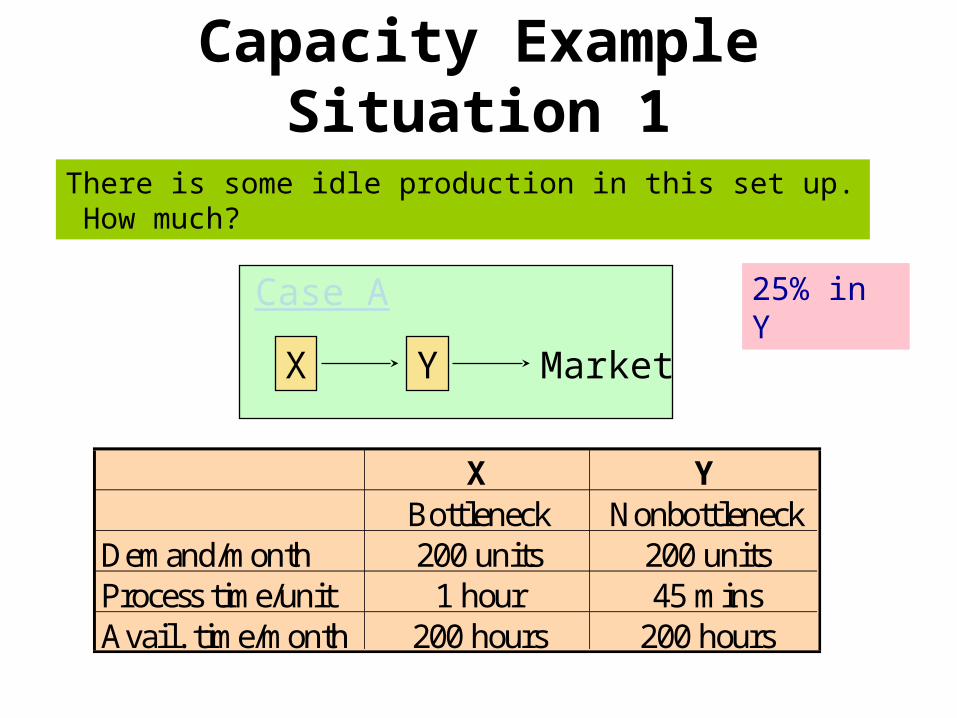
Capacity Example Situation 1
X Y Market
Case A
X YBottleneck Nonbottleneck
Demand/month 200 units 200 unitsProcess time/unit 1 hour 45 minsAvail. time/month 200 hours 200 hours
There is some idle production in this set up. How much?
25% in Y
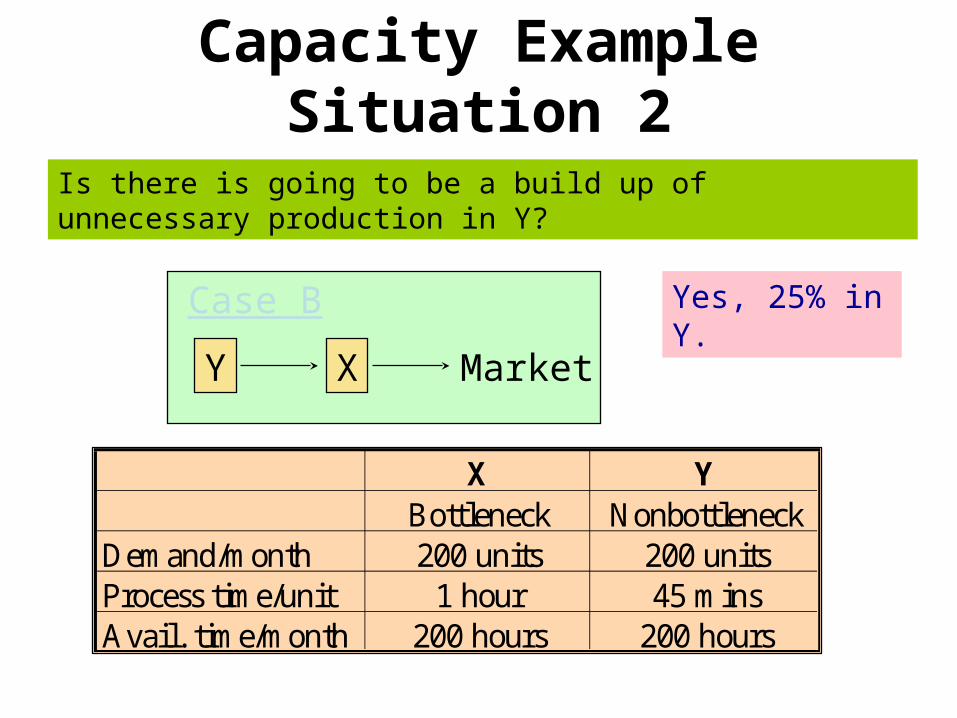
Capacity Example Situation 2
Y X Market
Case B
X YBottleneck Nonbottleneck
Demand/month 200 units 200 unitsProcess time/unit 1 hour 45 minsAvail. time/month 200 hours 200 hours
Is there is going to be a build up of unnecessary production in Y?
Yes, 25% in Y.
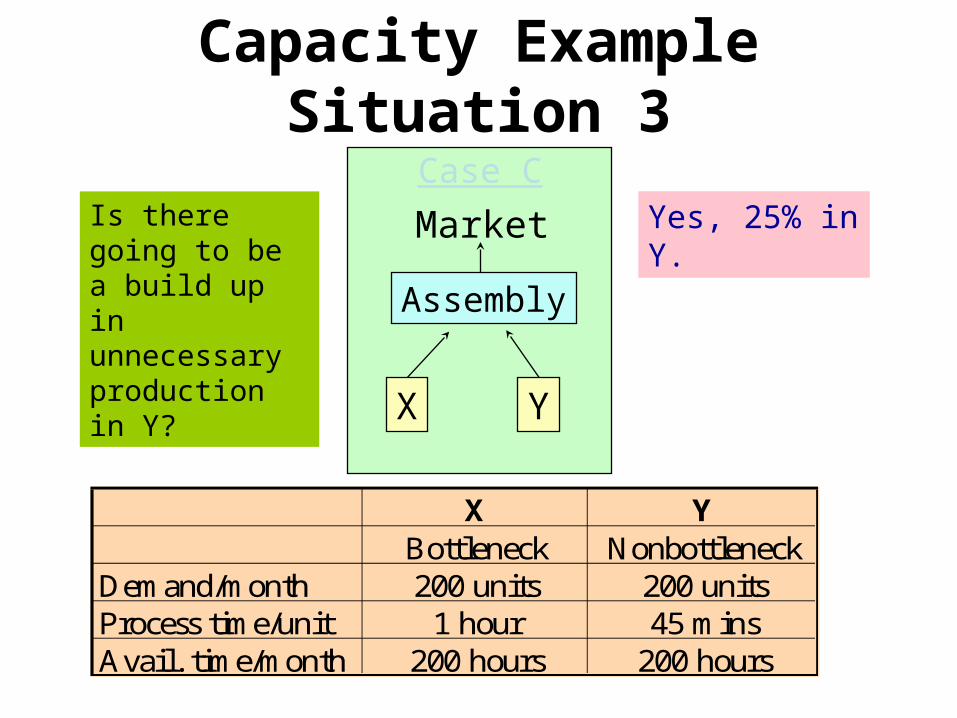
Capacity Example Situation 3
X Y
Assembly
Market
Case C
X YBottleneck Nonbottleneck
Demand/month 200 units 200 unitsProcess time/unit 1 hour 45 minsAvail. time/month 200 hours 200 hours
Is there going to be a build up in unnecessary production in Y?
Yes, 25% in Y.
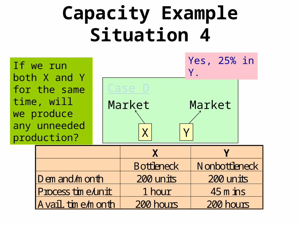
Capacity Example Situation 4
X Y
Market Market
Case D
X YBottleneck Nonbottleneck
Demand/month 200 units 200 unitsProcess time/unit 1 hour 45 minsAvail. time/month 200 hours 200 hours
If we run both X and Y for the same time, will we produce any unneeded production?
Yes, 25% in Y.
Time Components of Production Cycle
• Setup time is the time that a part spends waiting for a resource to be set up to work on this same part.
• Process time is the time that the part is being processed.
• Queue time is the time that a part waits for a resource while the resource is busy with something else.
Time Components of Production Cycle (Continued)• Wait time is the time that a part waits not
for a resource but for another part so that they can be assembled together.
• Idle time is the unused time. It represents the cycle time less the sum of the setup time, processing time, queue time, and wait time.
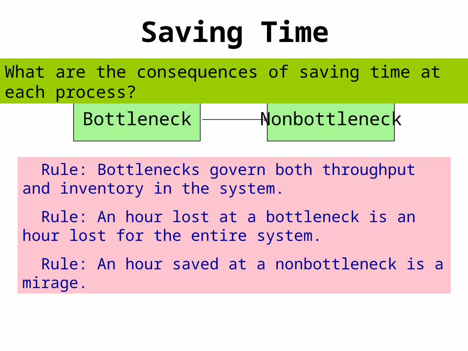
Saving Time
Bottleneck Nonbottleneck
What are the consequences of saving time at each process?
Rule: Bottlenecks govern both throughput and inventory in the system.
Rule: An hour lost at a bottleneck is an hour lost for the entire system.
Rule: An hour saved at a nonbottleneck is a mirage.
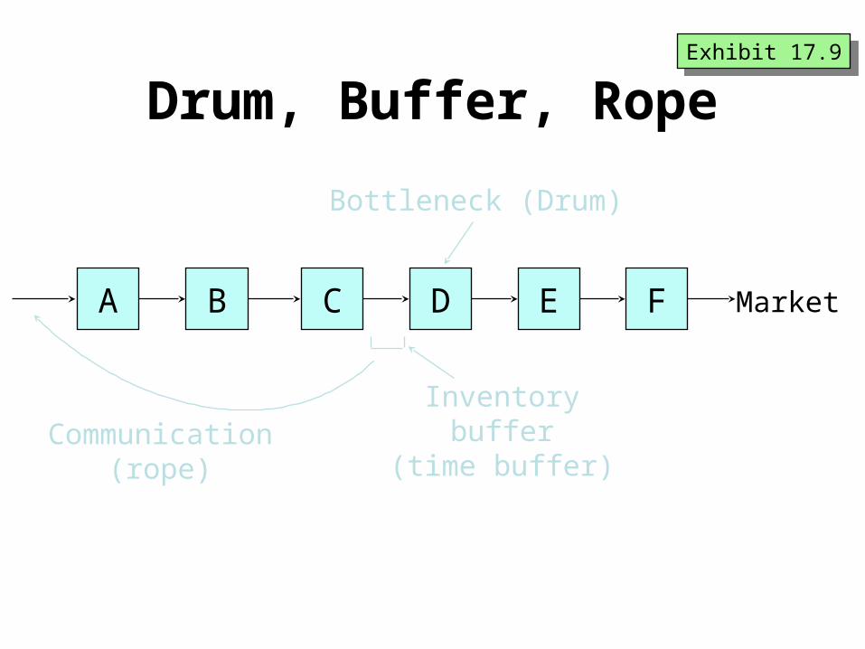
Drum, Buffer, Rope
A B C D E F
Bottleneck (Drum)
Inventorybuffer
(time buffer)Communication
(rope)
Market
Exhibit 17.9Exhibit 17.9
Quality Implications of synchronous manufacturing
• More tolerant than JIT systems– Excess capacity throughout system.
• Except for the bottleneck– Quality control needed before bottleneck.
Batch Sizes
• What is the batch size?
– One?
– Infinity?
Bottlenecks and CCRs:Flow-Control Situations
• A bottleneck – (1) with no setup required when changing from
one product to another.– (2) with setup times required to change from one
product to another.
• A capacity constrained resource (CCR)– (3) with no setup required to change from one
product to another.– (4) with setup time required when changing from
one product to another.
Inventory Cost Measurement:Dollar Days
• Dollar Days is a measurement of the value of inventory and the time it stays within an area.
Dollar Days = (value of inventory)(number of days within a department)
Example
Benefits from Dollar Day Measurement
• Marketing– Discourages holding large amounts of finished
goods inventory.
• Purchasing– Discourages placing large purchase orders that
on the surface appear to take advantage of quantity discounts.
• Manufacturing– Discourage large work in process and producing
earlier than needed.
Comparing Synchronous Manufacturing to MRP
• MRP uses backward scheduling.
• Synchronous manufacturing uses forward scheduling.
Comparing Synchronous Manufacturing to JIT
• JIT is limited to repetitive manufacturing
• JIT requires a stable production level
• JIT does not allow very much flexibility in the products produced