inventory management. inflow > outflow inflow < outflow inflow = outflow inventory the law of...
TRANSCRIPT
Inventory Management
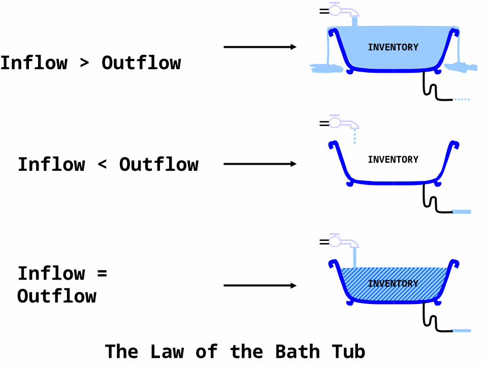
Inflow > Outflow
Inflow < Outflow
Inflow = Outflow
INVENTORY
INVENTORY
INVENTORY
The Law of the Bath Tub
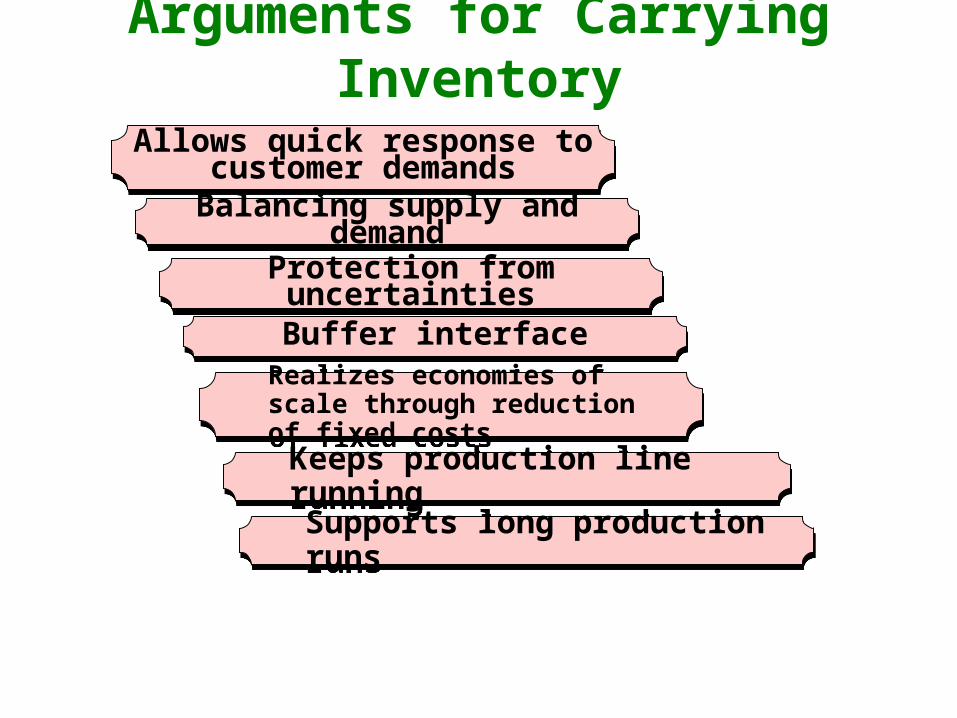
Arguments for Carrying Inventory
Balancing supply and demandBalancing supply and demand
Protection from uncertaintiesProtection from uncertainties
Buffer interfaceBuffer interface
Realizes economies of scale through reduction of fixed costs Realizes economies of scale through reduction of fixed costs
Allows quick response to customer demands
Allows quick response to customer demands
Keeps production line running Keeps production line running
Supports long production runsSupports long production runs
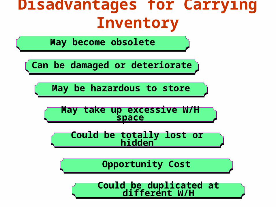
Disadvantages for Carrying Inventory
May become obsoleteMay become obsolete
Can be damaged or deteriorateCan be damaged or deteriorate
May be hazardous to storeMay be hazardous to store
May take up excessive W/H spaceMay take up excessive W/H space
Could be totally lost or hiddenCould be totally lost or hidden
Opportunity CostOpportunity Cost
Could be duplicated at different W/HCould be duplicated at different W/H
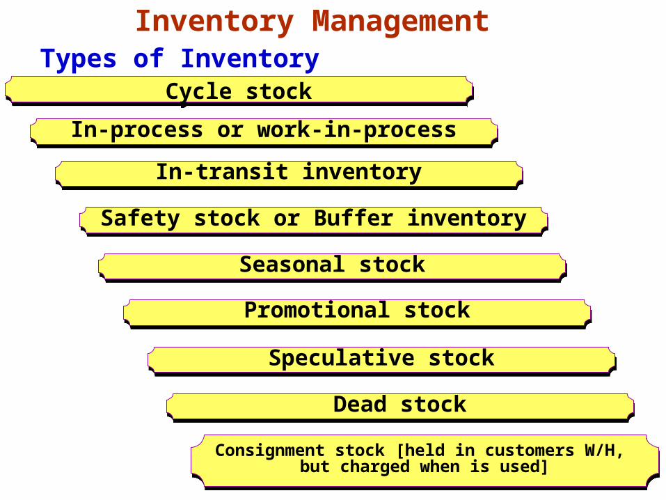
Cycle stockCycle stock
In-process or work-in-processIn-process or work-in-process
In-transit inventoryIn-transit inventory
Safety stock or Buffer inventorySafety stock or Buffer inventory
Seasonal stockSeasonal stock
Promotional stockPromotional stock
Speculative stockSpeculative stock
Dead stockDead stock
Consignment stock [held in customers W/H, but charged when is used]
Consignment stock [held in customers W/H, but charged when is used]
Types of Inventory
Inventory Management
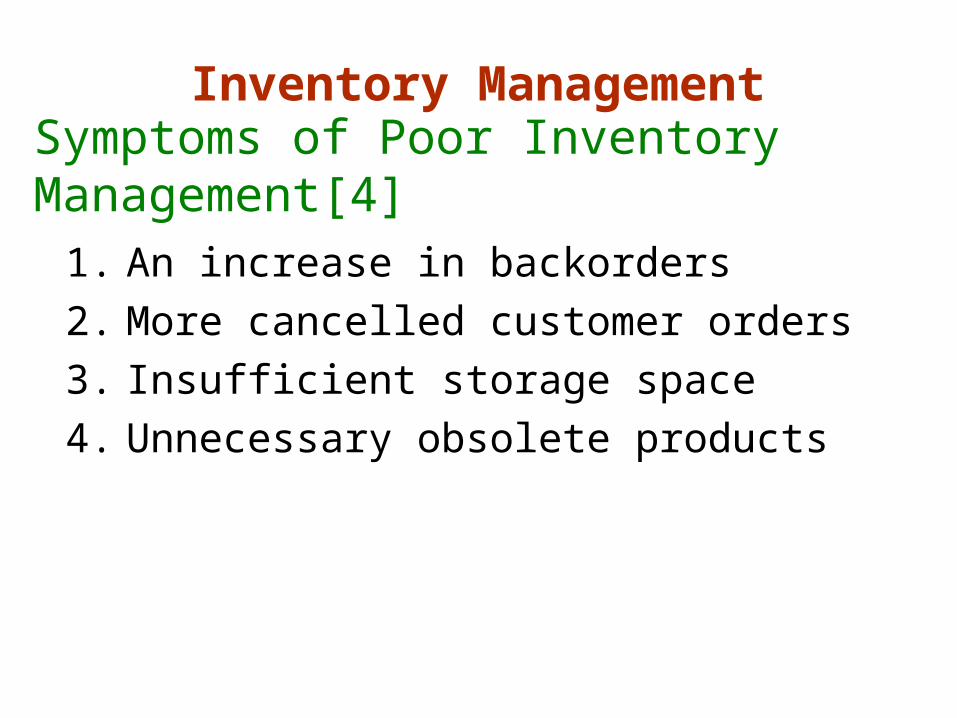
Symptoms of Poor Inventory Management[4]
1. An increase in backorders
2. More cancelled customer orders
3. Insufficient storage space
4. Unnecessary obsolete products
Inventory Management
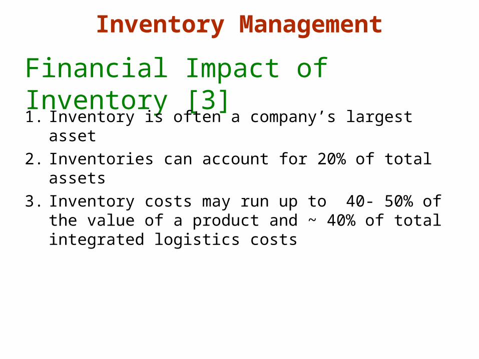
Financial Impact of Inventory [3]1. Inventory is often a company’s largest asset
2. Inventories can account for 20% of total assets
3. Inventory costs may run up to 40- 50% of the value of a product and ~ 40% of total integrated logistics costs
Inventory Management
Definitions
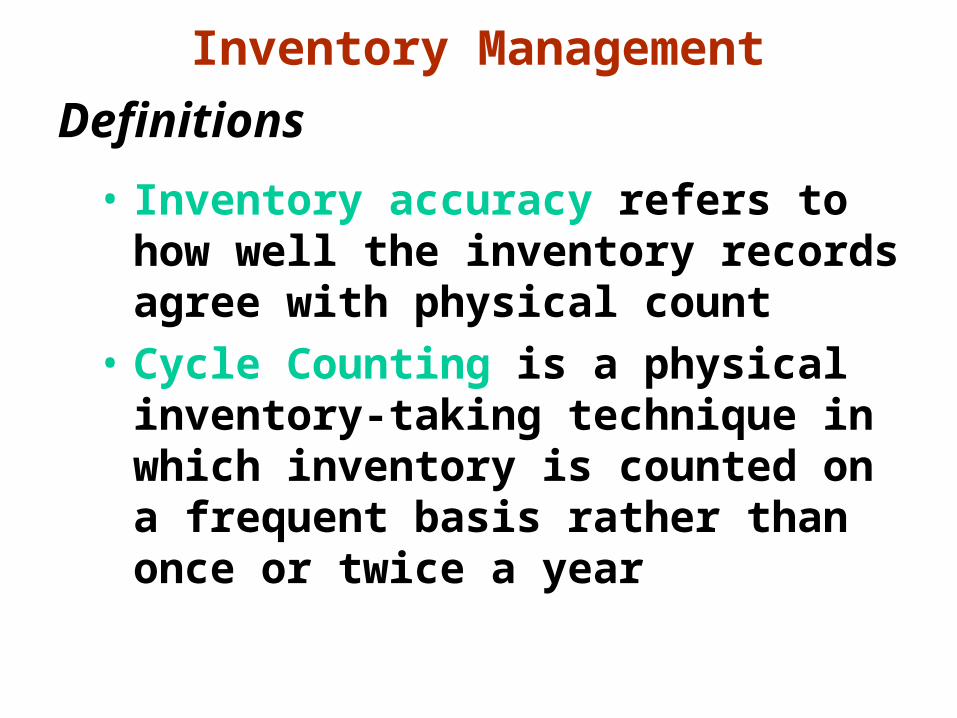
• Inventory accuracy refers to how well the inventory records agree with physical count
• Cycle Counting is a physical inventory-taking technique in which inventory is counted on a frequent basis rather than once or twice a year
Inventory Management
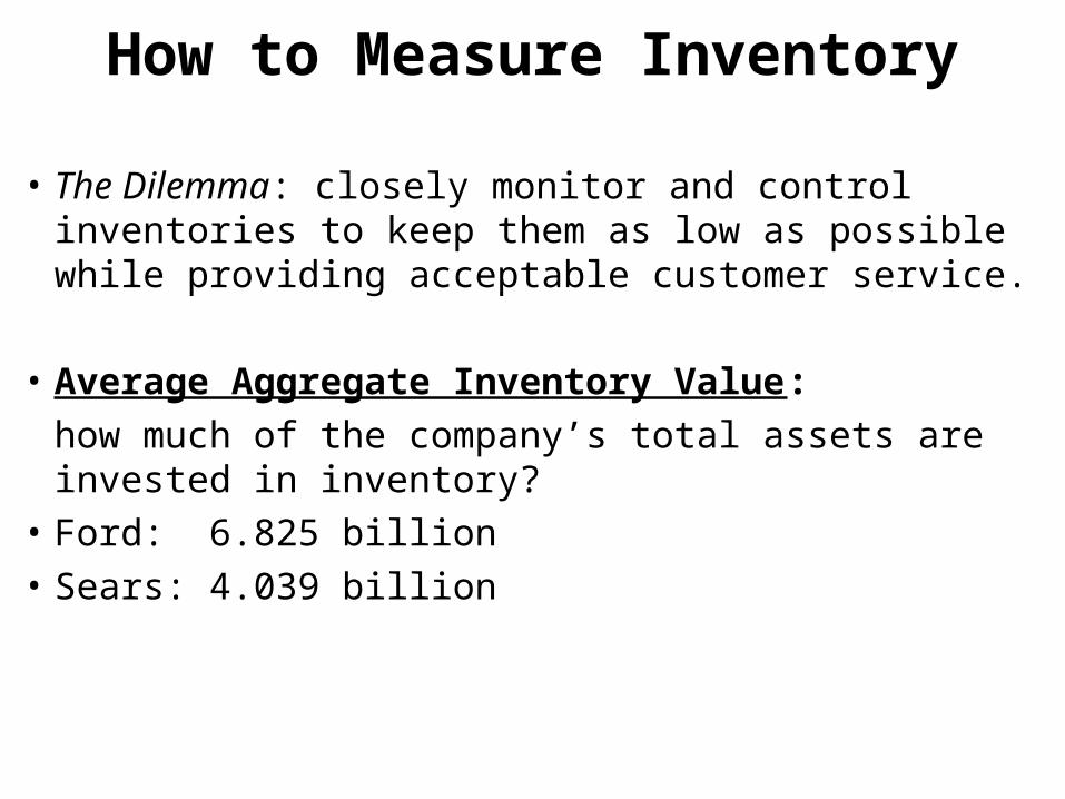
How to Measure Inventory
• The Dilemma: closely monitor and control inventories to keep them as low as possible while providing acceptable customer service.
• Average Aggregate Inventory Value:
how much of the company’s total assets are invested in inventory?
• Ford: 6.825 billion
• Sears: 4.039 billion
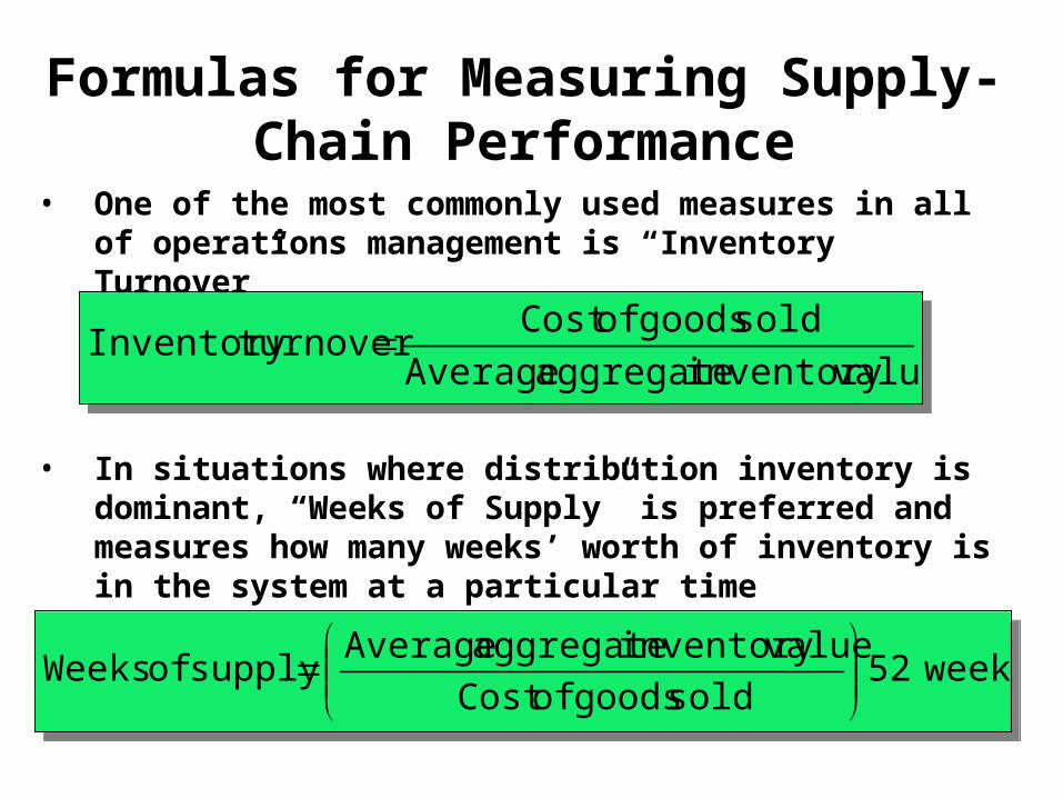
Formulas for Measuring Supply-Chain Performance
• One of the most commonly used measures in all of operations management is “Inventory Turnover”
• In situations where distribution inventory is dominant, “Weeks of Supply” is preferred and measures how many weeks’ worth of inventory is in the system at a particular time
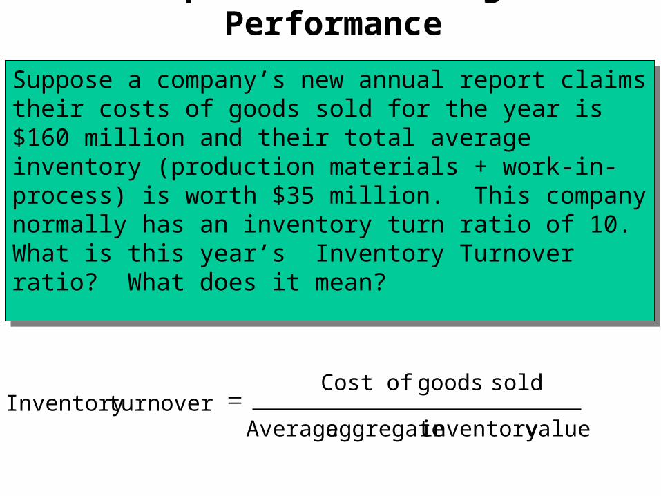
valueinventory aggregate Average
sold goods ofCost turnoverInventory valueinventory aggregate Average
sold goods ofCost turnoverInventory
weeks52 sold goods ofCost
valueinventory aggregate Averagesupply of Weeks
weeks52
sold goods ofCost
valueinventory aggregate Averagesupply of Weeks
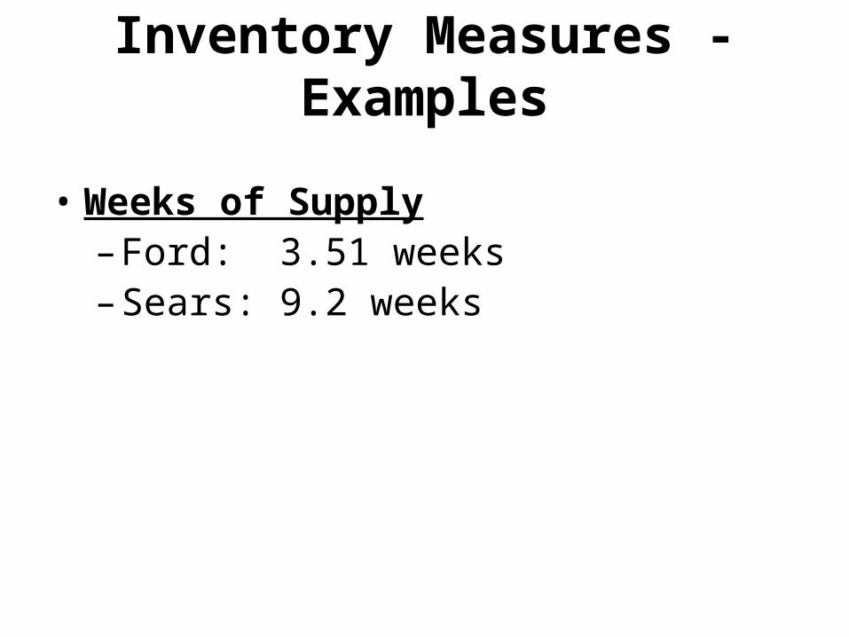
Inventory Measures - Examples
• Weeks of Supply– Ford: 3.51 weeks– Sears: 9.2 weeks
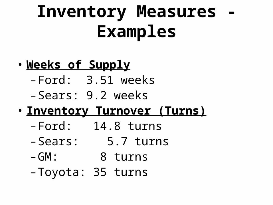
Inventory Measures - Examples
• Weeks of Supply– Ford: 3.51 weeks– Sears: 9.2 weeks
• Inventory Turnover (Turns)– Ford: 14.8 turns– Sears: 5.7 turns– GM: 8 turns– Toyota: 35 turns
Example of Measuring SC Performance
Suppose a company’s new annual report claims their costs of goods sold for the year is $160 million and their total average inventory (production materials + work-in-process) is worth $35 million. This company normally has an inventory turn ratio of 10. What is this year’s Inventory Turnover ratio? What does it mean?
Suppose a company’s new annual report claims their costs of goods sold for the year is $160 million and their total average inventory (production materials + work-in-process) is worth $35 million. This company normally has an inventory turn ratio of 10. What is this year’s Inventory Turnover ratio? What does it mean?
valueinventory aggregate Average
sold goods ofCost turnoverInventory
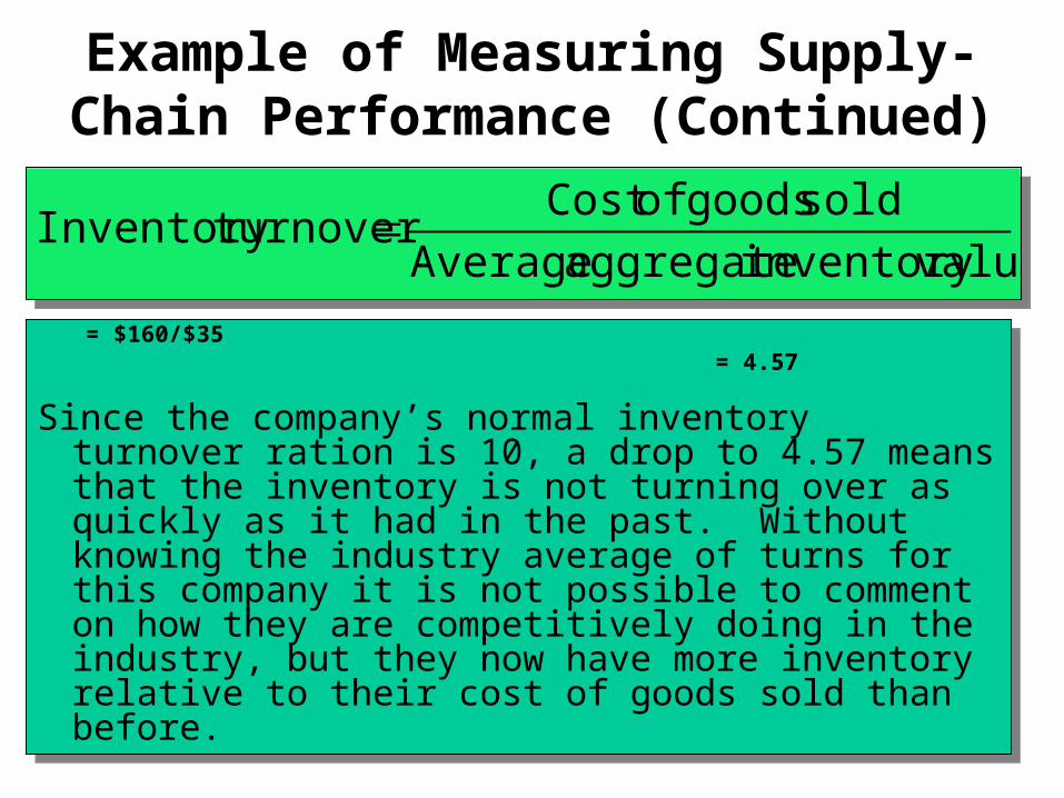
Example of Measuring Supply-Chain Performance (Continued)
= $160/$35 = 4.57
Since the company’s normal inventory turnover ration is 10, a drop to 4.57 means that the inventory is not turning over as quickly as it had in the past. Without knowing the industry average of turns for this company it is not possible to comment on how they are competitively doing in the industry, but they now have more inventory relative to their cost of goods sold than before.
valueinventory aggregate Average
sold goods ofCost turnoverInventory
valueinventory aggregate Average
sold goods ofCost turnoverInventory
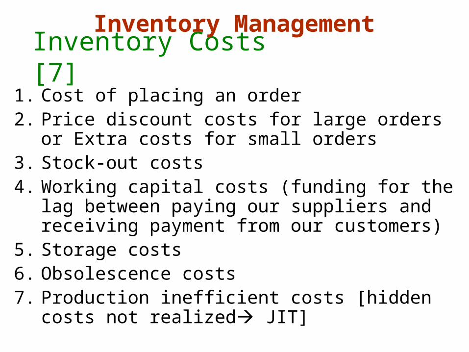
Inventory Costs [7]1. Cost of placing an order2. Price discount costs for large orders or Extra costs for
small orders3. Stock-out costs4. Working capital costs (funding for the lag between
paying our suppliers and receiving payment from our customers)
5. Storage costs6. Obsolescence costs7. Production inefficient costs [hidden costs not realized
JIT]
Inventory Management
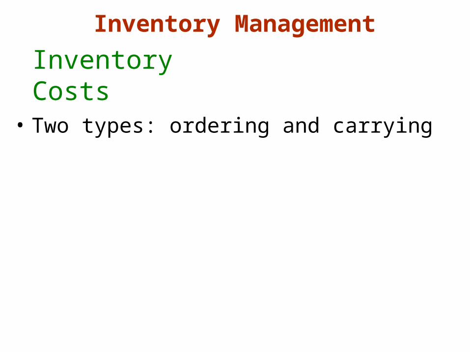
Inventory Costs
• Two types: ordering and carrying
Inventory Management
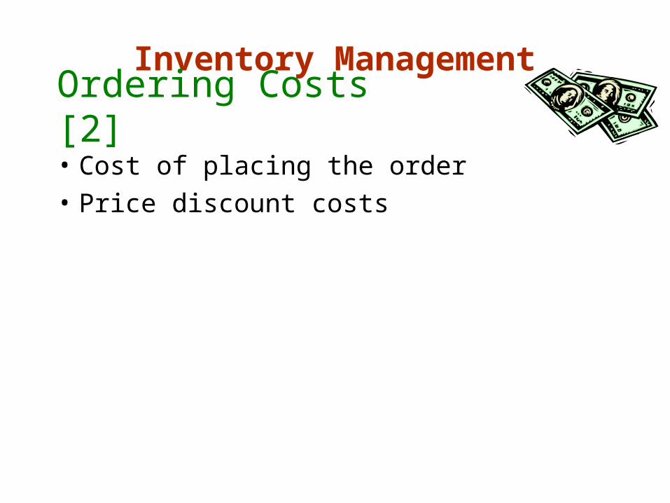
• Cost of placing the order
• Price discount costs
Inventory Management
Ordering Costs [2]
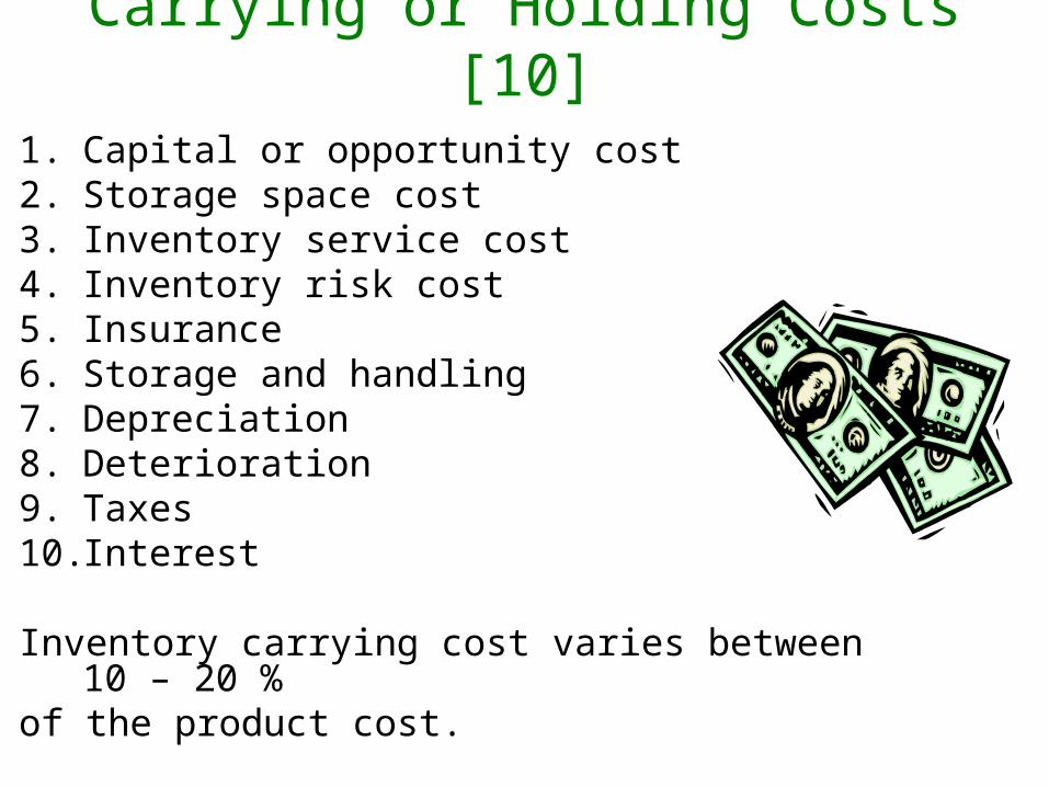
1. Capital or opportunity cost2. Storage space cost3. Inventory service cost4. Inventory risk cost5. Insurance6. Storage and handling7. Depreciation8. Deterioration9. Taxes10. Interest
Inventory carrying cost varies between 10 – 20 %of the product cost.
Carrying or Holding Costs [10]
Time
QO
n-ha
nd I
nven
tory
Time
Q
On-
hand
Inv
ento
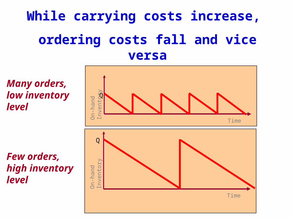
ryMany orders, low inventory level
Few orders, high inventory level
While carrying costs increase,
ordering costs fall and vice versa
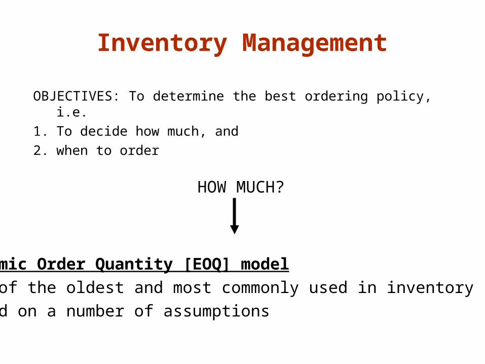
OBJECTIVES: To determine the best ordering policy, i.e.
1. To decide how much, and
2. when to order
Economic Order Quantity [EOQ] model
•One of the oldest and most commonly used in inventory control
•Based on a number of assumptions
HOW MUCH?
Inventory Management
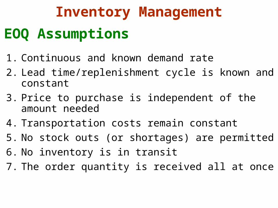
EOQ Assumptions
1. Continuous and known demand rate
2. Lead time/replenishment cycle is known and constant
3. Price to purchase is independent of the amount needed
4. Transportation costs remain constant
5. No stock outs (or shortages) are permitted
6. No inventory is in transit
7. The order quantity is received all at once
Inventory Management
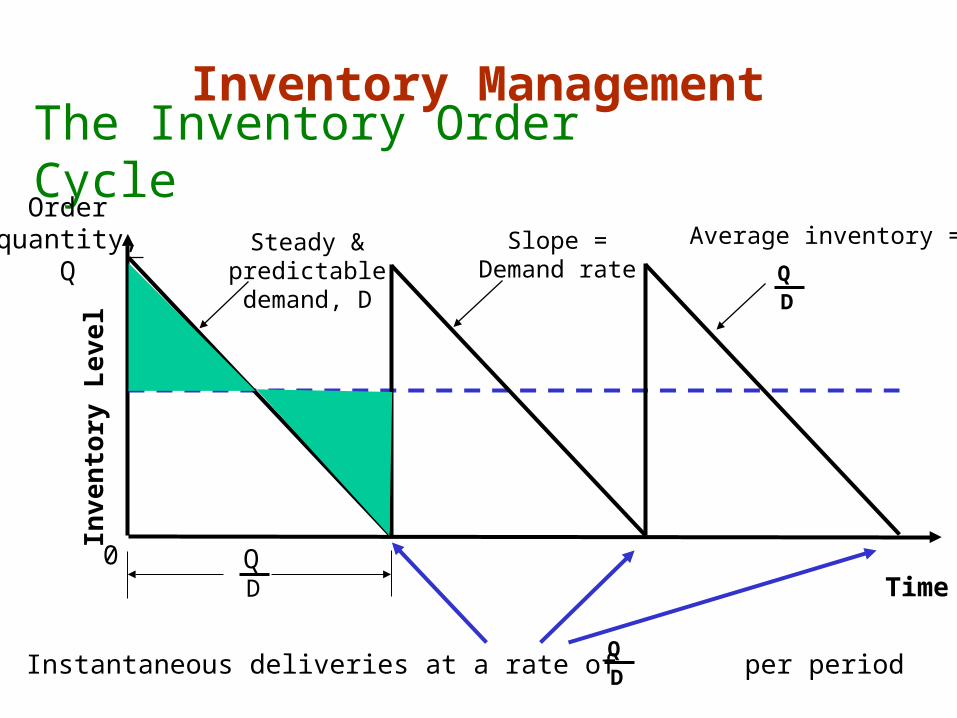
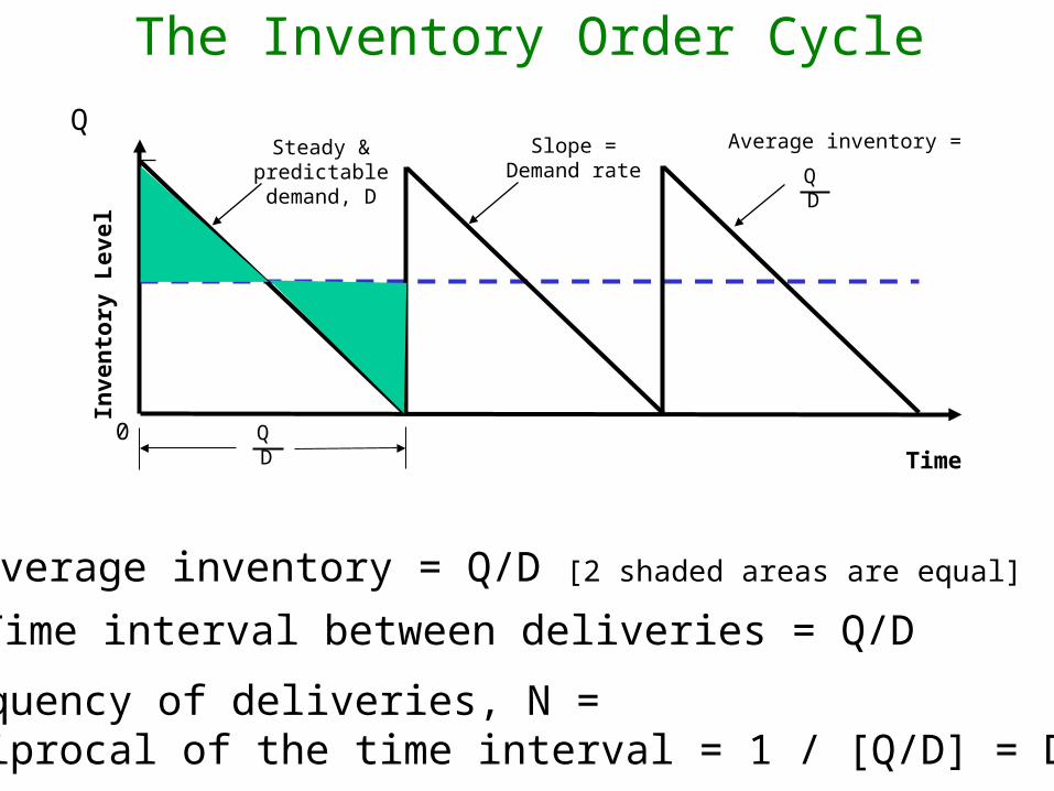
The Inventory Order Cycle
Steady &predictabledemand, D
0Time
Inve
nto
ry L
eve
l
Orderquantity,
Q
Inventory Management
QD
Slope =Demand rate
Average inventory =
QD
Instantaneous deliveries at a rate of per periodQD
The Inventory Order Cycle
Steady &predictabledemand, D
0Time
Inve
nto
ry L
evel
Q
QD
Slope =Demand rate
Average inventory =
QD
• Average inventory = Q/D [2 shaded areas are equal]
• Time interval between deliveries = Q/D
• Frequency of deliveries, N = reciprocal of the time interval = 1 / [Q/D] = D/Q
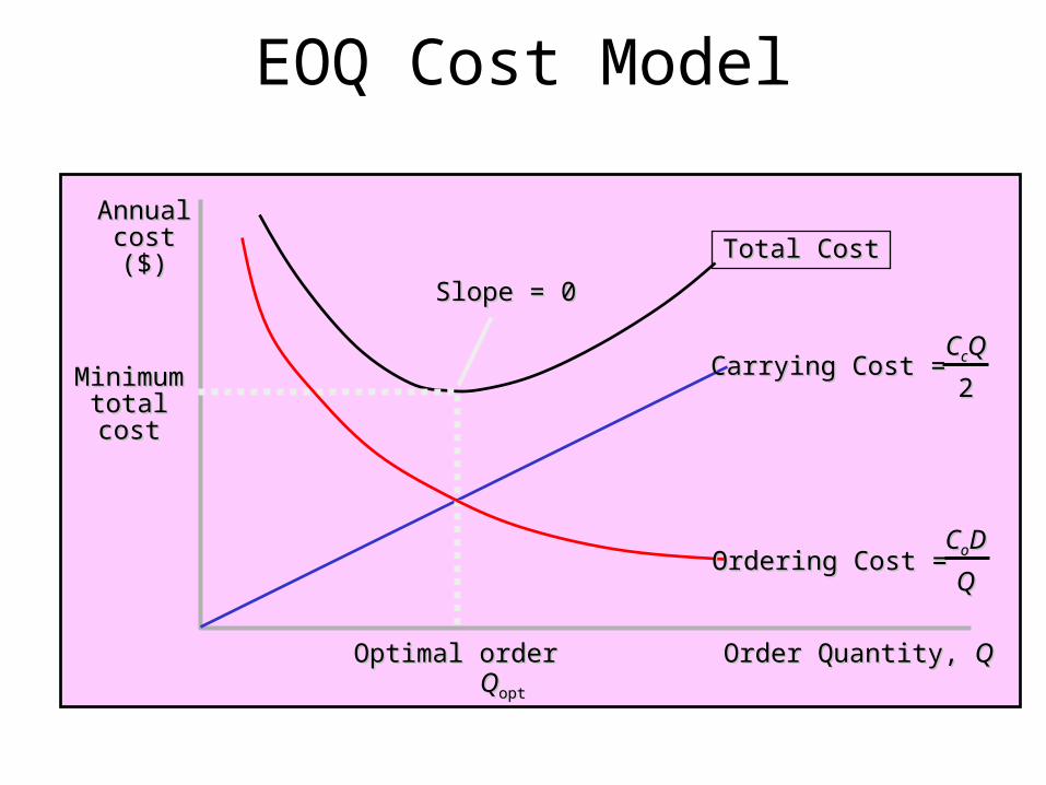
Order Quantity, Order Quantity, QQ
Annual Annual cost ($)cost ($) Total CostTotal Cost
Carrying Cost =Carrying Cost =CCccQQ
22
Slope = 0Slope = 0
Minimum Minimum total costtotal cost
Optimal orderOptimal order QQoptopt
Ordering Cost =Ordering Cost =CCooDD
EOQ Cost Model
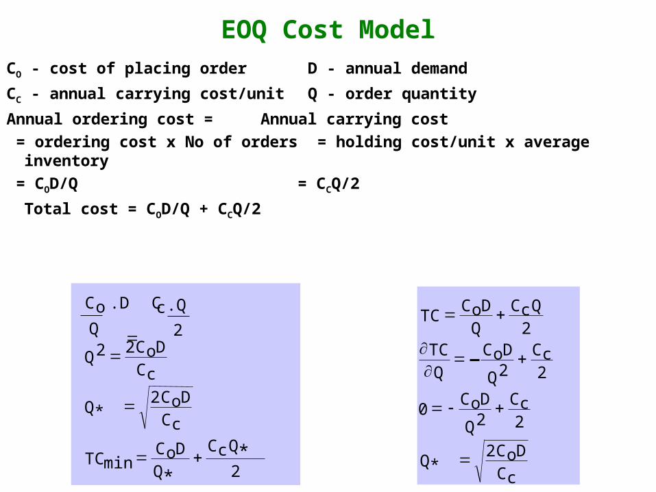
EOQ Cost Model
CO - cost of placing order D - annual demand
CC - annual carrying cost/unit Q - order quantity
Annual ordering cost = Annual carrying cost
= ordering cost x No of orders = holding cost/unit x average inventory
= COD/Q = CCQ/2
Total cost = COD/Q + CCQ/2
Co .D
Q
Cc .Q
QCoDCc
Q*CoDCc
TCCoDQ*
CcQ*
22 2
2
2min
TCCoD
QCcQ
TCQ
CoD
Q
Cc
CoD
Q
Cc
Q*CoDCc
2
2 2
02 2
2
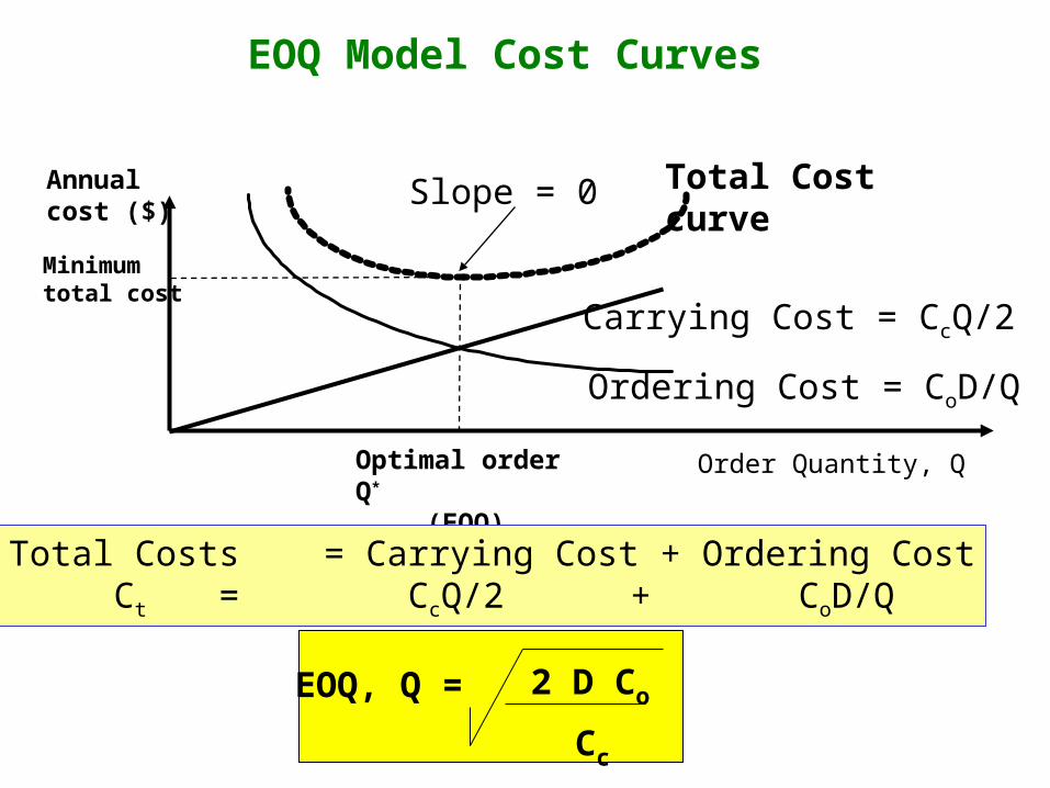
EOQ Model Cost Curves
Slope = 0 Total Costcurve
Ordering Cost = CoD/Q
Order Quantity, Q
Annualcost ($)
Minimumtotal cost
Optimal order Q*
(EOQ)
Carrying Cost = CcQ/2
Total Costs = Carrying Cost + Ordering CostCt = CcQ/2 + CoD/Q
EOQ, Q = 2 D Co
Cc
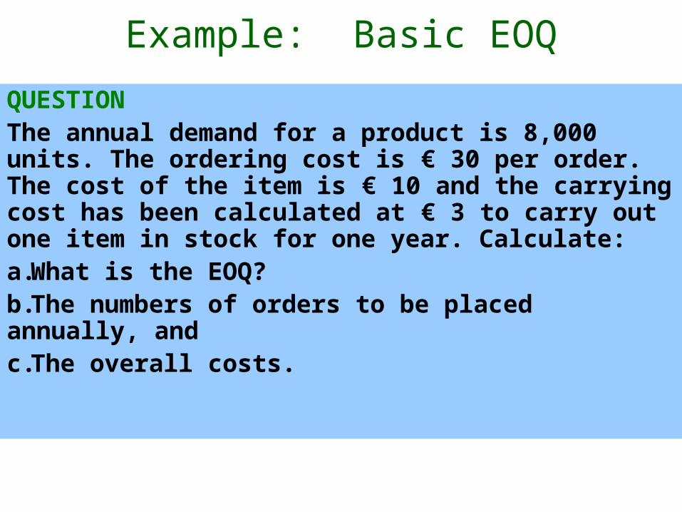
QUESTIONThe annual demand for a product is 8,000 units. The ordering cost is € 30 per order. The cost of the item is € 10 and the carrying cost has been calculated at € 3 to carry out one item in stock for one year. Calculate:a.What is the EOQ?b.The numbers of orders to be placed annually, andc.The overall costs.
Example: Basic EOQ
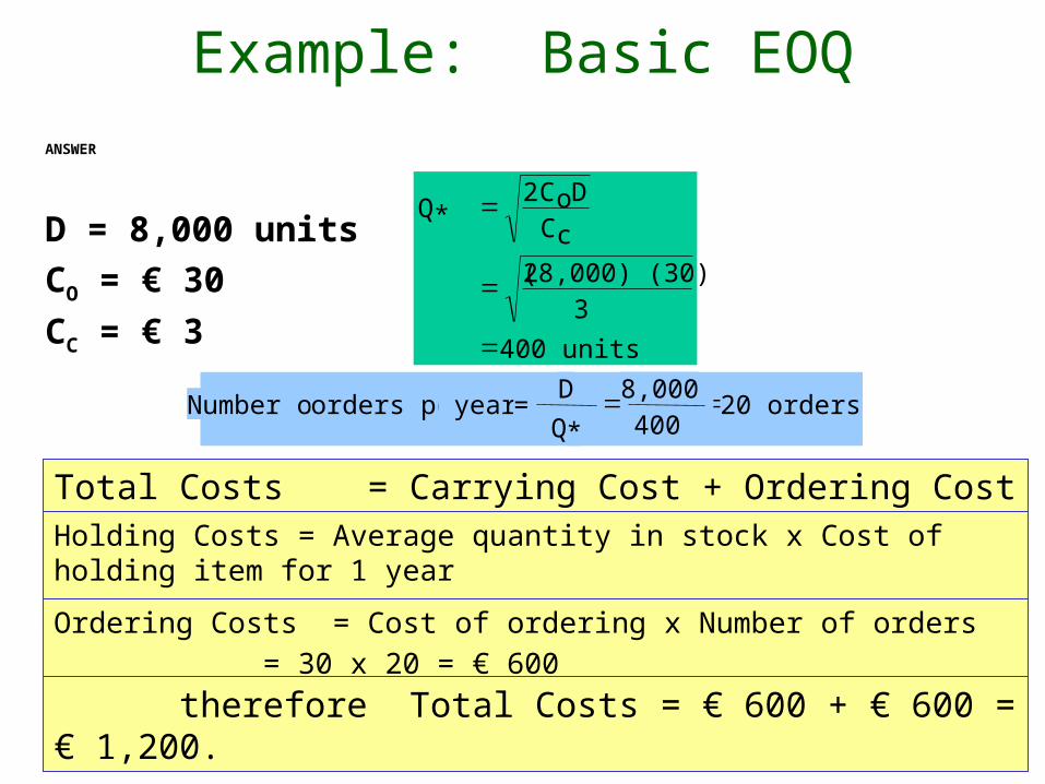
ANSWER
D = 8,000 units
CO = € 30
CC = € 3
Q*CoDCc
2
2 (8,000) (30)3
400 units
Number of orders per year =D
Q* 8,000
40020 orders
Total Costs = Carrying Cost + Ordering Cost Holding Costs = Average quantity in stock x Cost of holding item for 1 year
= 400/2 x 3 = € 600 Ordering Costs = Cost of ordering x Number of orders
= 30 x 20 = € 600 therefore Total Costs = € 600 + € 600 = € 1,200.
Example: Basic EOQ
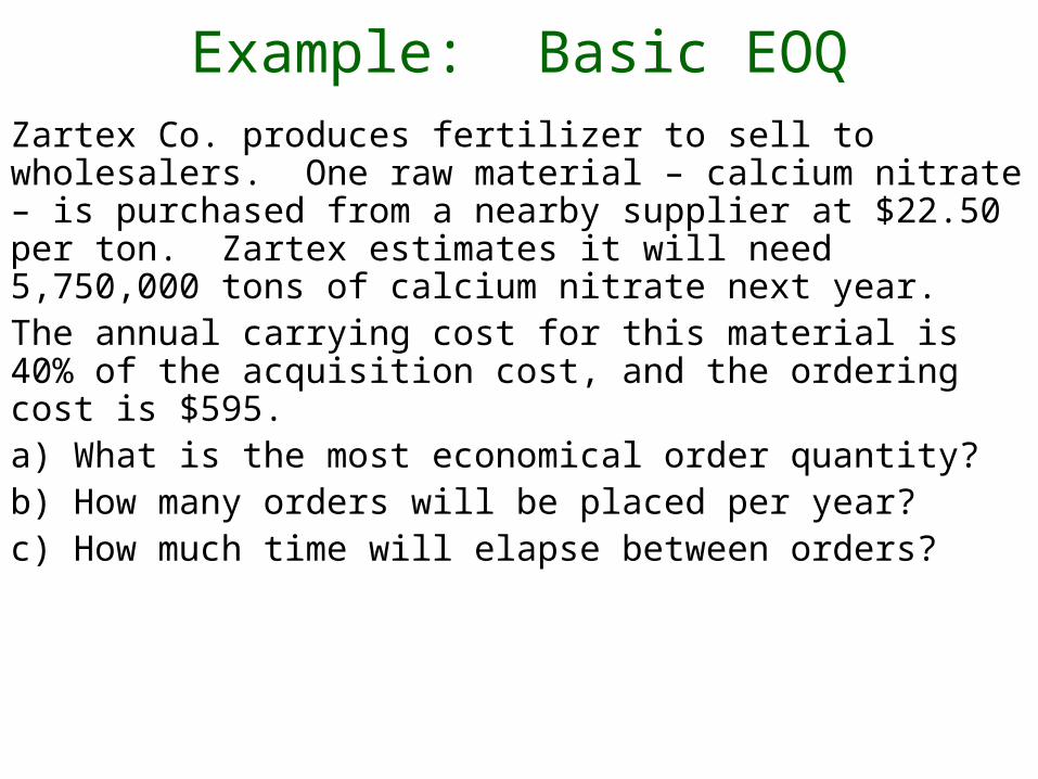
Zartex Co. produces fertilizer to sell to wholesalers. One raw material – calcium nitrate – is purchased from a nearby supplier at $22.50 per ton. Zartex estimates it will need 5,750,000 tons of calcium nitrate next year.The annual carrying cost for this material is 40% of the acquisition cost, and the ordering cost is $595. a) What is the most economical order quantity?b) How many orders will be placed per year?c) How much time will elapse between orders?
Example: Basic EOQ
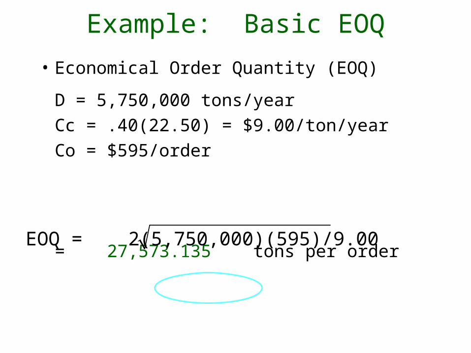
• Economical Order Quantity (EOQ)
D = 5,750,000 tons/year
Cc = .40(22.50) = $9.00/ton/year
Co = $595/order
= 27,573.135 tons per order
Example: Basic EOQ
EOQ = 2(5,750,000)(595)/9.00
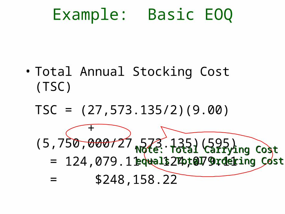
• Total Annual Stocking Cost (TSC)
TSC = (27,573.135/2)(9.00)
+ (5,750,000/27,573.135)(595)
= 124,079.11 + 124,079.11
= $248,158.22 Note: Total Carrying CostNote: Total Carrying Costequals Total Ordering Costequals Total Ordering Cost
Example: Basic EOQ
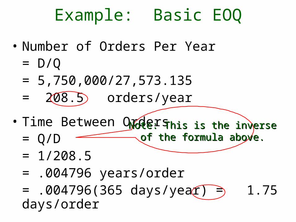
• Number of Orders Per Year= D/Q = 5,750,000/27,573.135 = 208.5 orders/year
• Time Between Orders= Q/D= 1/208.5= .004796 years/order= .004796(365 days/year) = 1.75
days/order
Note: This is the inverseNote: This is the inverse of the formula above.of the formula above.
Example: Basic EOQ
END